Embed Size (px)
Citation preview
BEAUTY IS A BEAST, FROG IS A PRINCE:
ASSORTATIVE MATCHINGWITH
NONTRANSFERABILITIES∗
Patrick Legros†and Andrew F. Newman‡
April 2002; revised: December 2006
Abstract
We present sufficient conditions for monotone matching in environments whereutility is not fully transferable between partners. These conditions involve not onlycomplementarity in types of the total payoff to a match, as in the transferable utilitycase, but also monotonicity in type of the degree of transferability between part-ners. We apply our conditions to study some models of risk sharing and incentiveproblems, deriving new results for predicted matching patterns in those contexts.
Keywords: Assortative matching, nontransferable utility, risk sharing, intrahouse-hold allocation, principal-agent.JEL Numbers: C78, D13, J41
∗We thank Ken Binmore, Patrick Bolton, Maristella Botticini, Bengt Holmstrom, Hide Ichimura,
Boyan Jovanovic, Eric Maskin, Meg Meyer, Nicola Pavoni, Wolfgang Pesendorfer, Ilya Segal, Lones
Smith, a co-editor and three anonymous referees, as well as seminar participants at Berkeley, Bonn,
BU, Caltech, Gerzensee, Harvard/MIT, Northwestern, Princeton, Stanford, Toulouse, UCL, UCSD,
UCSB, and ULB, for useful comments and discussion.
†ECARES, Université Libre de Bruxelles, Avenue F.D. Roosevelt 50, C.P. 114, 1050 Brussels, Bel-
gium: [email protected], http://homepages.ulb.ac.be/~plegros, and CEPR. This author benefited from
the financial support of the Communauté française de Belgique (projects ARC 98/03-221and ARC00/05-
252) and EU TMR Network contract no FMRX-CT98-0203.
‡Boston University, Department of Economics, 270 Bay State Road, Boston, MA 02215, USA :
[email protected]; and CEPR. This author acknowledges support as the Richard B. Fisher Member,
Institute for Advanced Study, Princeton, and as a Peter B. Kenen Fellow, Department of Economics,
Princeton University.
1. Introduction
For the economist analyzing household behavior, firm formation, or the labor market,
the characteristics of matched partners are paramount. The educational background
of men and women who are married, the financial positions of firms that are merging,
or the productivities of agents who are working together, all matter for understanding
their respective markets. Matching patterns serve as direct evidence for theory, figure in
the econometrics of selection effects, facilitate theoretical analysis, and are even treated
as policy variables.
Much is known about characterizing matching in the special case of transferable
utility (TU). For instance, if the function representing the total payoff to the match
satisfies increasing (decreasing) differences in the partners’ attributes, then there will
always be positive (negative) assortative matching, whatever the distribution of types.
Because they are distribution-free, results of this sort are very powerful and easy to
apply.
But in many areas of economic analysis, the utility among individuals is not fully
transferable (“non-transferable,” or NTU). Partners may be risk averse with limited
insurance possibilities; incentive or enforcement problems may restrict the way in which
the joint output can be divided; or policy makers may impose rules about how output
may be shared within relationships. As Becker (1973) pointed out long ago, rigidities
that prevent partners from costlessly dividing the gains from a match may change the
matching outcome, even if the level of output continues to satisfy monotone differences
in type.
While interest in the issues represented by the non-transferable case is both long-
standing and lively (see for instance Farrell and Scotchmer, 1988 on production in
partnerships; Rosenzweig and Stark, 1989 on risk sharing in households; and more
recently, Lazear, 2000 on incentive schemes for workers; Ackerberg and Botticini, 2002
on sharecropping; and Besley and Ghatak, 2005 on the organizational design of nonprofit
firms), for the analyst seeking to characterize the equilibrium matching pattern in such
settings, there is little theoretical guidance.
1

The purpose of this paper is to offer some. We present sufficient conditions for
assortative matching that are simple to express, intuitive to understand, and, we hope,
tractable to apply. We illustrate their use with some examples that are of independent
interest.
The class of models we consider are two-person matching games without search fric-
tions in which the utility possibility frontier for any pair of agents is a strictly decreasing
function. After introducing the model, we review the logic of the classical transferable
utility results, which leads us to propose the “generalized difference conditions” (GDC)
that suffice to guarantee monotone matching for any type distribution (Proposition 1).
We also present sufficient differential conditions for monotone matching (Corollary
1). In addition to being straightforward to verify, the differential conditions offer addi-
tional insight into the forces governing matching. In particular, they highlight the role
not only of the complementarity in partners’ types that figures in the TU case, but also
of a complementarity between an agent’s type and his partner’s payoff that is the new
feature in the NTU case. This second complementarity entails that the degree of trans-
ferability (i.e., slope of the frontier) be monotone in type. Even if the output satisfies
increasing differences in types, failure of the type-payoff complementarity may overturn
the predictions of the TU model and lead instead to negative assortative matching or
some more complex and/or distribution-dependent pattern.
Two examples illustrate the application of our general results. The first is a mar-
riage market model in which partners vary in risk attitude and must share risks within
their households. Sorting effects in this kind of model are important considerations in
the econometrics of marriage and migration (Rosenzweig and Stark, 1989). Using the
GDC, we show that partners will sort negatively in their Arrow-Pratt degree of risk
tolerance. The differential conditions are applied to the second example, a principal-
agent model in which agents vary in their initial wealth, and principals vary in the
riskiness of their projects. Matching effects in such a model are of direct interest in
some applications (e.g., Newman, 1999; Prendergast, 2002) and have been offered as
explanations for some seemingly puzzling empirical results (Ackerberg and Botticini,
2
2002). In this example, the type-transferability relationship alone is responsible for the
predicted matching pattern, which goes in a (possibly) unexpected direction.
Finally, we discuss the strength of the GDC, pointing out that they are ordinal con-
ditions (Proposition 2), which broadens the scope of applicability of the local conditions;
that they are necessary if one seeks a distribution-free condition for assortative match-
ing (Proposition 3); and their distinction from established conditions in the literature
(Sections 6.3 and 7.3). Section 7 discusses extensions of our results to variations of the
standard matching framework, and Section 8 concludes.
The next section delves further into the ideas underlying the general theoretical
analysis by examining a very simple example inspired by the one in Becker (1973).
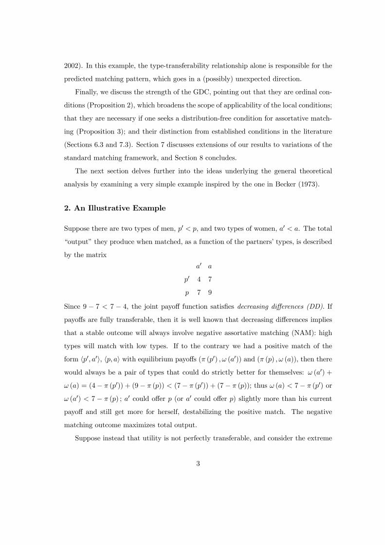
2. An Illustrative Example
Suppose there are two types of men, p0 < p, and two types of women, a0 < a. The total
“output” they produce when matched, as a function of the partners’ types, is described
by the matrix
a0 a
p0 4 7
p 7 9
Since 9 − 7 < 7 − 4, the joint payoff function satisfies decreasing differences (DD). If
payoffs are fully transferable, then it is well known that decreasing differences implies
that a stable outcome will always involve negative assortative matching (NAM): high
types will match with low types. If to the contrary we had a positive match of the
form hp0, a0i, hp, ai with equilibrium payoffs (π (p0) , ω (a0)) and (π (p) , ω (a)), then there
would always be a pair of types that could do strictly better for themselves: ω (a0) +
ω (a) = (4− π (p0)) + (9− π (p)) < (7− π (p0)) + (7− π (p)); thus ω (a) < 7− π (p0) or
ω (a0) < 7 − π (p) ; a0 could offer p (or a0 could offer p) slightly more than his current
payoff and still get more for herself, destabilizing the positive match. The negative
matching outcome maximizes total output.
Suppose instead that utility is not perfectly transferable, and consider the extreme
3
case in which any departure from equal sharing within the marriage is impossible. For
instance, the payoff to the marriage could be generated by the joint consumption of a
local public good. Thus each partner in hp, ai gets 4.5, each in hp, a0i gets 3.5, etc. Now
the only stable outcome is positive assortative matching (PAM): each p is better off
matching with a (4.5) than with a0 (3.5), and thus the “power couple” blocks a negative
assortative match. As Becker noted, with nontransferability, the match changes, and
aggregate performance suffers as well.
Of course this extreme form of nontransferability does not represent many situations
of economic interest. What happens in the broad intermediate range? Introduce a dose
of transferability by supposing that some compensation, say through the return of favors,
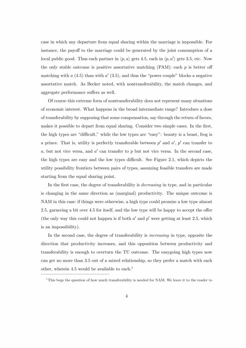
makes it possible to depart from equal sharing. Consider two simple cases. In the first,
the high types are “difficult,” while the low types are “easy”: beauty is a beast, frog is
a prince. That is, utility is perfectly transferable between p0 and a0, p0 can transfer to
a, but not vice versa, and a0 can transfer to p but not vice versa. In the second case,
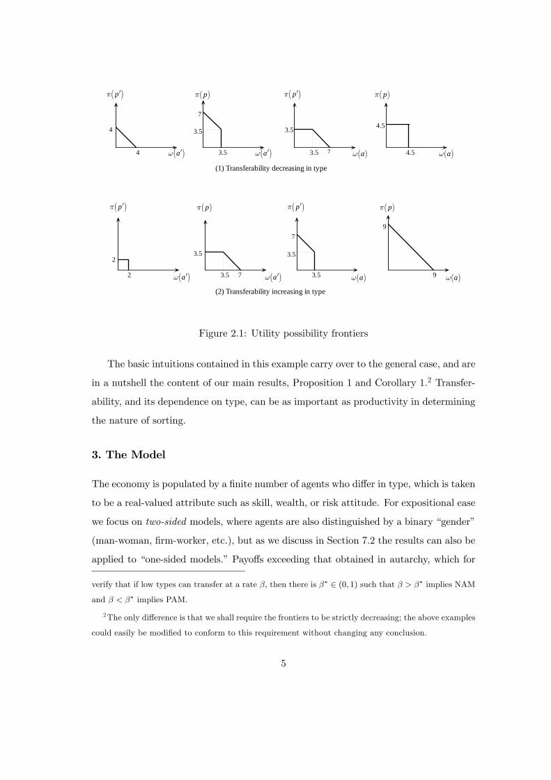
the high types are easy and the low types difficult. See Figure 2.1, which depicts the
utility possibility frontiers between pairs of types, assuming feasible transfers are made
starting from the equal sharing point.
In the first case, the degree of transferability is decreasing in type, and in particular
is changing in the same direction as (marginal) productivity. The unique outcome is
NAM in this case: if things were otherwise, a high type could promise a low type almost
2.5, garnering a bit over 4.5 for itself, and the low type will be happy to accept the offer
(the only way this could not happen is if both a0 and p0 were getting at least 2.5, which
is an impossibility).
In the second case, the degree of transferability is increasing in type, opposite the
direction that productivity increases, and this opposition between productivity and
transferability is enough to overturn the TU outcome. The easygoing high types now
can get no more than 3.5 out of a mixed relationship, so they prefer a match with each
other, wherein 4.5 would be available to each.1
1This begs the question of how much transferability is needed for NAM. We leave it to the reader to
4
(1) Transferability decreasing in type
(2) Transferability increasing in type
4
4
7
3.5
3.5
7
4.5
4.5
2
2
3.5
7
7
3.5
9
9
3.5
3.5
3.5
3.5
( )aω
( )aω ′
( )pπ( )pπ ′ ( )pπ ′
( )pπ ′( )pπ ′
( )pπ
( )pπ( )pπ
( )aω ′
( )aω ′( )aω ′ ( )aω
( )aω( )aω
Figure 2.1: Utility possibility frontiers
The basic intuitions contained in this example carry over to the general case, and are
in a nutshell the content of our main results, Proposition 1 and Corollary 1.2 Transfer-
ability, and its dependence on type, can be as important as productivity in determining
the nature of sorting.
3. The Model
The economy is populated by a finite number of agents who differ in type, which is taken
to be a real-valued attribute such as skill, wealth, or risk attitude. For expositional ease
we focus on two-sided models, where agents are also distinguished by a binary “gender”
(man-woman, firm-worker, etc.), but as we discuss in Section 7.2 the results can also be
applied to “one-sided models.” Payoffs exceeding that obtained in autarchy, which for
verify that if low types can transfer at a rate β, then there is β∗ ∈ (0, 1) such that β > β∗ implies NAM
and β < β∗ implies PAM.
2The only difference is that we shall require the frontiers to be strictly decreasing; the above examples
could easily be modified to conform to this requirement without changing any conclusion.
5
the general analysis we normalize to zero for all types,3 are generated only if agents of
opposite gender match.
Let I be the set of agents on one side of the market and J be the set of agents on
the other. The description of a specific economy includes an assignment of individuals
to types via maps ρ : I −→ P, and α : J −→ A, where P and A are compact subsets of
R. To simplify the exposition we assume that I and J have the same cardinality.4
The object of analytical interest is the utility possibility frontier (since in equilibrium
agents will always select an allocation on this frontier) for each possible pairing of agents.
This frontier will be represented by a bounded continuous function φ : P×A×R+ → R+;
φ(p, a, v) denotes the maximum utility generated by a type p ∈ P in a match with a type
a ∈ A who receives utility v. The maximum equilibrium payoff that p could ever get in
a match with a is φ(p, a, 0), since a would never accept a negative payoff. We assume
throughout that φ (p, a, 0) is positive for all (p, a) and that φ(p, a, v) is continuous and
strictly decreasing in v whenever φ (p, a, v) is positive.5
Let ψ (a, p, ·) be the “quasi-inverse” of φ (p, a, ·): ψ (a, p, u) is the maximum payoff
to a type-a when his type-p partner receives utility u. For any p ∈ P, a ∈ A, if u ∈
[0, φ(p, a, 0)], ψ (a, p, u) solves φ (p, a, ψ (a, p, u)) = u, and if u > φ(p, a, 0), ψ(a, p, u) = 0.
3 In many applications, the autarchy payoff varies with type. The analysis extends to this case almost
without modification: see Section 7.1.
4This is basically without loss of generality; see Section 7.1.
5While we take φ to be a primitive of the model for the general analysis, it will typically be derived
from more fundamental assumptions about technology, preferences and choices made by the partners
after they match, as in the examples in Section 5. The frontier can be generally expressed as
φ(p, a, v) = maxx
U(x, p, a)
s.t. V (x, a, p) ≥ v
x ∈ Ω(p, a),
where U is the utility of the agent in I, V the utility of the agent in J, x the choice variables, and
Ω (p, a) ⊂ Rn is the choice set. The frontier will have the indicated properties if, for instance, U and V
are continuous and locally nonsatiated, Ω (p, a) is continuous, and for each (p, a) , Ω (p, a) has nonempty
relative interior and contains a point xpa such that U (xpa, p, a) > 0, V (xpa, a, p) > 0.
6

In general, of course, φ(p, a, w) 6= ψ(a, p, w).
We shall sometimes refer to the first argument of φ and ψ as “own type,” the second
argument as “partner’s type,” and the third argument as “payoff.”
The notation reflects two further assumptions of matching models, namely (1) that
the payoff possibilities depend only on the types of the agents and not on their individual
identities; and (2) the utility possibilities of the pair of agents do not depend on what
other agents in the economy are doing, i.e., there are no externalities across coalitions.
The model encompasses the case of transferable utility (TU), in which there exists
a production function h (a, p) such that φ (p, a, v) can be written as h(p, a) − v for
v ∈ [0, h(p, a)]. In all other cases we have nontransferable utility (NTU).
Our concept of equilibrium is the core of the assignment game: it requires that
agents in I are matched to agents in J in a stable way.
Definition 1. Payoffs (u, v) are feasible for (p, a) ∈ P × A if u ≤ φ (p, a, v) and v ≤
ψ (a, p, 0) .
Definition 2. An equilibrium specifies a one-to-one matching function m : I → J and
payoff allocations π∗ : I −→ R+ and ω∗ : J −→ R+ that satisfy the two following
conditions.
(i) Feasibility of (π∗, ω∗) with respect to m : for all i ∈ I, (π∗ (i) , ω∗ (m (i))) is feasible
for (ρ (i) , α (m (i))).
(ii) Stability ofm with respect to (π∗, ω∗) : there do not exist (i, j) ∈ I×J and v > ω∗ (j)
such that φ (ρ (i) , α (j) , v) > π∗ (i) .
Existence of equilibria in this class of economies has been established elsewhere
(Kaneko, 1982).
Because φ (p, a, v) is strictly decreasing in v on (0, ψ (a, p, 0)) , an equilibrium satis-
fies equal treatment: if two agents with the same type had unequal equilibrium payoffs,
it would be possible for the worse-treated to underbid the better-treated, contradicting
stability. Thus, the equilibrium payoff functions π∗ and ω∗ depend only on the individ-
ual’s type, and it is enough to define type-dependent payoff functions π : P → R+ and
7
ω : A → R+ as π (p) = π∗ (ρ (i)) when ρ (i) = p for i ∈ I and ω (a) = ω∗ (α (j)) when
α (j) = a for j ∈ J.
Concepts of monotone matching are defined with respect to the matching corre-
spondence between types. The matching function m : I → J generates a matching
correspondence on types M: P ⇒ A :
M (p) = α (j) , j ∈ J : ∃i ∈ I, ρ (i) = p and j = m (i) .
We say thatM is stable given (π, ω) if there do not exist (p, a) and v > ω (a) such that
φ (p, a, v) > π (p).
When M is a monotone correspondence, matching is monotone. In two-sided mod-
els, there are only two types of monotone matching. An equilibrium displays positive
assortative matching (PAM) if p > p0, a ∈ M (p) , a0 ∈ M (p0) =⇒ a ≥ a0. There is
negative assortative matching (NAM) if p > p0, a ∈M (p) , a0 ∈M (p0) =⇒ a0 ≥ a.
Say that an equilibrium is payoff equivalent to another if all agents have the same
payoff in each equilibrium. We say an economy satisfies PAM (NAM) if each equilibrium
is payoff equivalent to one in which the match satisfies PAM (NAM).
4. Sufficient Conditions for Monotone Matching
4.1. Logic of the TU Case
Recall the conventional transferable utility result, as that will provide guidance to the
general case. In the TU case, only the total payoff h(p, a) is relevant. The assumption
that is often made about h is that it satisfies increasing differences (ID): whenever
p > p0 and a > a0, h(p, a)− h(p, a0) ≥ h(p0, a)− h(p0, a0). Why does this imply positive
assortative matching, irrespective of the distribution of types? Usually, the argument is
made by noticing that the total output among the four types is maximized (a necessary
condition of equilibrium in the TU case, but not, we should emphasize, in the case of
NTU) when p matches with a and p0 with a0: this is evident from rearranging the ID
condition.
8
However, it is more instructive to analyze this from the equilibrium point of view.
Suppose that a and a0 compete for the right to match with p rather than p0. The in-
creasing difference condition says that a can outbid a0 in this competition, since the
incremental output produced if a switches to p exceeds that when a0 switches. In par-
ticular, this is true whatever the level of utility u that p0 might be receiving: rewrite
(strict) ID as h(p, a)− [h(p0, a)− u] > h(p, a0)− [h(p0, a0)− u]; this is literally the state-
ment that a’s willingness to pay for p, given that p0 is getting u, exceeds a0’s. Thus a
situation in which p is matched with a0 and p0 with a is never stable: a will be happy to
offer more to p than the latter is getting with a0. The ID result is distribution free: the
type distribution will affect the equilibrium payoffs, but the argument just given shows
that p’s partner must be larger than p0’s regardless of what those payoffs might be.
The convenient feature of TU is that if a outbids a0 at one level of u, he does so for all
u. Such is not the case with NTU. Our sufficient condition will require explicitly that a
can outbid a0 for all relevant levels of u. If this requirement seems strong, recall that the
nature of the result sought, namely monotone matching regardless of the distribution,
is also strong. By the same token, it is weaker than ID, and includes TU as a special
case.
In an NTU model, the division of the surplus between the partners cannot be sep-
arated from the level that they generate. Switching to a higher type partner may not
be attractive if it is also more costly to transfer utility to a high type, that is, if the
frontier is steeper. A sufficient condition for PAM is that not only there is the usual
type-type complementarity in the production of surplus, but also there is a type-payoff
complementarity: frontiers are flatter, as well as higher, for higher types. This will
perhaps be more apparent from the local form of our conditions.
4.2. Generalized Difference Conditions
Let p > p0 and a > a0 and suppose that p0 were to get u. Then the above reasoning
would suggest that a would be able to outbid a0 for p given that p0 has a given outside
9
option of u :
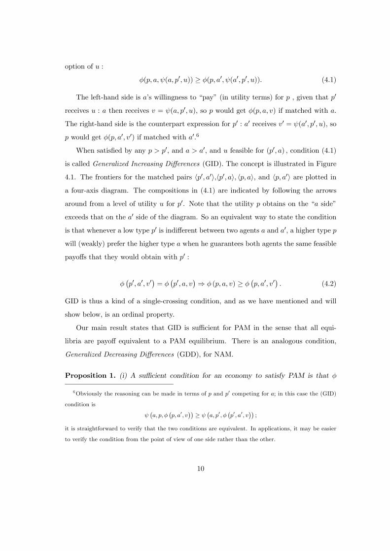
φ(p, a, ψ(a, p0, u)) ≥ φ(p, a0, ψ(a0, p0, u)). (4.1)
The left-hand side is a’s willingness to “pay” (in utility terms) for p , given that p0
receives u : a then receives v = ψ(a, p0, u), so p would get φ(p, a, v) if matched with a.
The right-hand side is the counterpart expression for p0 : a0 receives v0 = ψ(a0, p0, u), so
p would get φ(p, a0, v0) if matched with a0.6
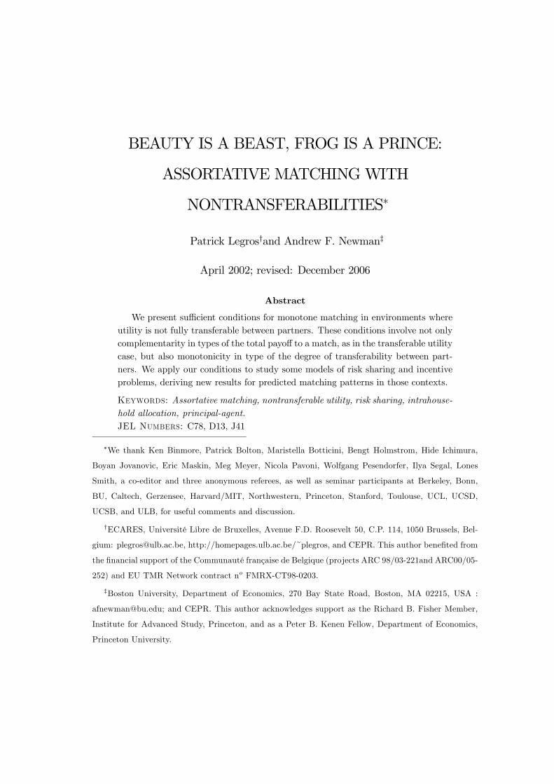
When satisfied by any p > p0, and a > a0, and u feasible for (p0, a) , condition (4.1)
is called Generalized Increasing Differences (GID). The concept is illustrated in Figure
4.1. The frontiers for the matched pairs hp0, a0i,hp0, ai, hp, ai, and hp, a0i are plotted in
a four-axis diagram. The compositions in (4.1) are indicated by following the arrows
around from a level of utility u for p0. Note that the utility p obtains on the “a side”
exceeds that on the a0 side of the diagram. So an equivalent way to state the condition
is that whenever a low type p0 is indifferent between two agents a and a0, a higher type p
will (weakly) prefer the higher type a when he guarantees both agents the same feasible
payoffs that they would obtain with p0 :
φ¡p0, a0, v0
¢= φ
¡p0, a, v
¢⇒ φ (p, a, v) ≥ φ
¡p, a0, v0
¢. (4.2)
GID is thus a kind of a single-crossing condition, and as we have mentioned and will
show below, is an ordinal property.
Our main result states that GID is sufficient for PAM in the sense that all equi-
libria are payoff equivalent to a PAM equilibrium. There is an analogous condition,
Generalized Decreasing Differences (GDD), for NAM.
Proposition 1. (i) A sufficient condition for an economy to satisfy PAM is that φ
6Obviously the reasoning can be made in terms of p and p0 competing for a; in this case the (GID)
condition is
ψ a, p, φ p, a0, v ≥ ψ a, p0, φ p0, a0, v ;
it is straightforward to verify that the two conditions are equivalent. In applications, it may be easier
to verify the condition from the point of view of one side rather than the other.
10

u
( )aω
( )pπ( )pπ ′
( )aω ′
( )( ), , , ,p a a p uφ ψ ′
( )( ), , , ,p a a p uφ ψ′ ′ ′
v
v′
Figure 4.1: Generalized Increasing Differences
satisfies generalized increasing differences (GID) : whenever p > p0, a > a0, and u ∈
[0, φ (p0, a, 0)], φ (p, a, ψ(a, p0, u)) ≥ φ (p, a0, ψ(a0, p0, u)) .
(ii) A sufficient condition for an economy to satisfy NAM is that φ satisfies gener-
alized decreasing differences (GDD) : whenever p > p0, a > a0, and u ∈ [0, φ(p0, a0, 0)],
φ (p, a, ψ(a, p0, u)) ≤ φ (p, a0, ψ(a0, p0, u)) .
The basic logic of the proof is very simple, particularly when GID holds strictly.
Suppose that contrary to PAM there is an equilibrium with types p > p0 and a > a0 that
are matched negatively, i.e., hp0, ai and hp, a0i. Feasibility entails that π(p0) ≤ φ(p0, a, 0),
so by strict GID,
φ¡p, a, ψ(a, p0, π
¡p0¢)¢> φ
¡p, a0, ψ(a0, p0, π
¡p0¢)¢.
Stability requires that a0 does not want to switch to p0, and a does not want to switch
11

to p :
ω(a0) = ψ(a0, p, π(p)) ≥ ψ(a0, p0, π(p0))
ω(a) = ψ(a, p0, π(p0)) ≥ ψ(a, p, π(p))
Applying φ(p, a0, ·) to both sides of the first inequality and φ(p, a, ·) to the second yields
(the inequalities are reversed since the operators are decreasing)
π(p) = φ(p, a0, ψ(a0, p, π(p))) ≤ φ(p, a0, ψ(a0, p0, π(p0)))
φ(p, a, ψ(a, p0, π(p0))) ≤ φ(p, a, ψ(a, p, π(p))) ≤ π(p);
thus φ(p, a, ψ(a, p0, π(p0))) ≤ φ(p, a0, ψ(a0, p0, π(p0))), contradicting strict GID. The full
proof considers the general case in which GID doesn’t hold strictly and where there may
exist equilibria which do not satisfy PAM; in this case we show that there is a payoff
equivalent PAM equilibrium. Details are in the Appendix.
4.3. The Differentiable Case
We now present a set of cross-partial derivative conditions. For this subsection, suppose
that P and A are nondegenerate closed intervals. Let
D = (p, a, v) ∈ R3 : p ∈ P, a ∈ A, v ∈ (0, ψ(a, p, 0))
be the “domain of nondegeneracy” of φ, that is for each pair (p, a) , we ignore the corner
values 0 and ψ(a, p, 0).
We shall also assume that each agent benefits from matching with a higher type
partner.
Definition 3. φ is type increasing if for all (p, a) ∈ P × A,u, v ∈ R+, φ (p, a, v) is
nondecreasing in a and ψ (a, p, u) is nondecreasing in p.
Note that φ type increasing implies that φ and ψ are nondecreasing in own type as
well as partner type.7
7Consider a > a. By definition, for u ∈ [0, φ(p, a, 0)], we have u = φ (p, a, ψ (a, p, u)) =
12

Corollary 1. Suppose φ is type increasing and twice continuously differentiable on D.
(i) A sufficient condition for the economy to satisfy PAM is that for all (p, a, v) ∈ D,
φ12(p, a, v) ≥ 0 and φ13(p, a, v) ≥ 0. (4.3)
(ii) A sufficient condition for the economy to satisfy NAM is that for all (p, a, v) ∈ D,
φ12(p, a, v) ≤ 0 and φ13(p, a, v) ≤ 0. (4.4)
The proof exploits the cross partial assumptions and the fact that φ is type increasing
to ensure that the marginal value of own type φ1(p, a, ψ(a, p0, u)) is monotone in a for
p ∈ [p0, p], and then integrates over p to obtain the GDC conditions. See the Appendix.
Obviously, with TU, φ13 = 0, so (4.3) reduces to the standard condition in that
case. The extra term reflects the fact that changing the type results in a change in the
slope of the frontier. For PAM, the idea is that higher types can transfer utility to their
partners more easily (φ3 is less negative, hence flatter).
The conditions in Corollary 1 illustrate the separate roles of both the usual type-type
complementarity and the type-payoff complementarity we have mentioned. In terms of
the bidding story we mentioned in Section 4.1, if two different types are competing for
a higher type partner, both will be willing to offer her more than they would a partner
with a lower type (φ2 > 0); if the higher type’s frontier is flatter than the lower’s frontier
(φ13 ≥ 0), it will cost the higher type less to do this than it will the lower one; meanwhile
if the high type is also more productive on the margin (φ12 > 0) then he is sure to win,
in effect being both more productive and having lower costs.
Remark 1. The GID condition states that whenever p > p0 and u ∈ [0, φ (p0, a, 0)] , the
function φ (p, a, ψ (a, p0, u)) is nondecreasing in a. Thus it is (almost) immediate that
φ (p, a, ψ (a, p, u)) . Since φ is nondecreasing in a, φ (p, a, ψ(a, p, u)) ≤ φ ((p, a, ψ(a, p, u)) , hence
φ (p, a, ψ(a, p, u)) ≤ φ (p, a, ψ (a, p, u)) which implies that ψ(a, p, u) ≥ ψ (a, p, u) since φ is decreasing in
payoff.
13

if φ is type increasing and continuously differentiable on D, a necessary and sufficient
condition for GID is
φ2(p, a, ψ(a, p0, u)) + φ3(p, a, ψ(a, p
0, u)) · ψ1(a, p0, u) ≥ 0 (4.5)
for all types p, p0 ∈ P with p ≥ p0 and all a ∈ A and utilities u ∈ (0, φ (p0, a, 0)) (see
Appendix). However, it appears that in practice, this condition would be more difficult
to verify than (4.3).
5. Applications
In this section we present two examples that are representative of those considered in
the literature and use them to illustrate the application of our general results. The first
is a marriage market model in which partners vary in risk attitude and must share risks
within their households. The second is a principal-agent model in which agents vary by
wealth and principals by project risk.
5.1. Risk Sharing in Households
Consider a marriage market model in which the primary desideratum in choosing a mate
is suitability for risk sharing. There are two sides to the market for households, and we
denote by p the characteristics of the men and by a the characteristics of the women.
Household production is random, with two possible outcomes w2 > w1 > 0, and associ-
ated probabilities q2 and q1. Everyone is an expected utility maximizer; income y yields
utility U(p, y) to a man of type p and V (a, y) to a woman of type a. Unmatched agents
get utility zero. For all p and a, U and V are twice differentiable, strictly increasing, and
strictly concave in income, with the marginal utility of income becoming unbounded as
income approaches zero. The characteristics p and a are interpreted as the indices of
absolute of risk tolerance: if p > p0, then −U22(p, y)/U2(p, y) < −U22(p0, y)/U2(p0, y) for
all y, and a > a0 implies −V22(a, y)/V2(a, y) < −V22(a0, y)/V2(a0, y) for all y. By Pratt’s
theorem, U(p, ·) is a strict convexification of U(p0, ·), and V (a, ·) is a strict convexifica-
tion of V (a0, ·).
14
For informational or enforcement reasons, the only risk sharing possibilities in this
economy lie within a household consisting of two agents. When partners match, their
(explicit or implicit) contract sii=1,2 specifies how each realization of the output will
be shared between them: si goes to the woman in state i, and the remaining wi − si
goes to the man.
For a household (p, a), the maximum expected utility the man can achieve if the
woman requires expected utility v is given by the value φ of the optimal risk sharing
problem:
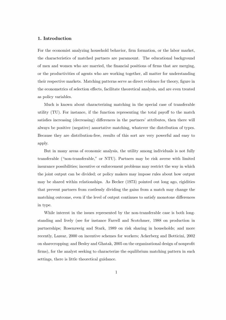
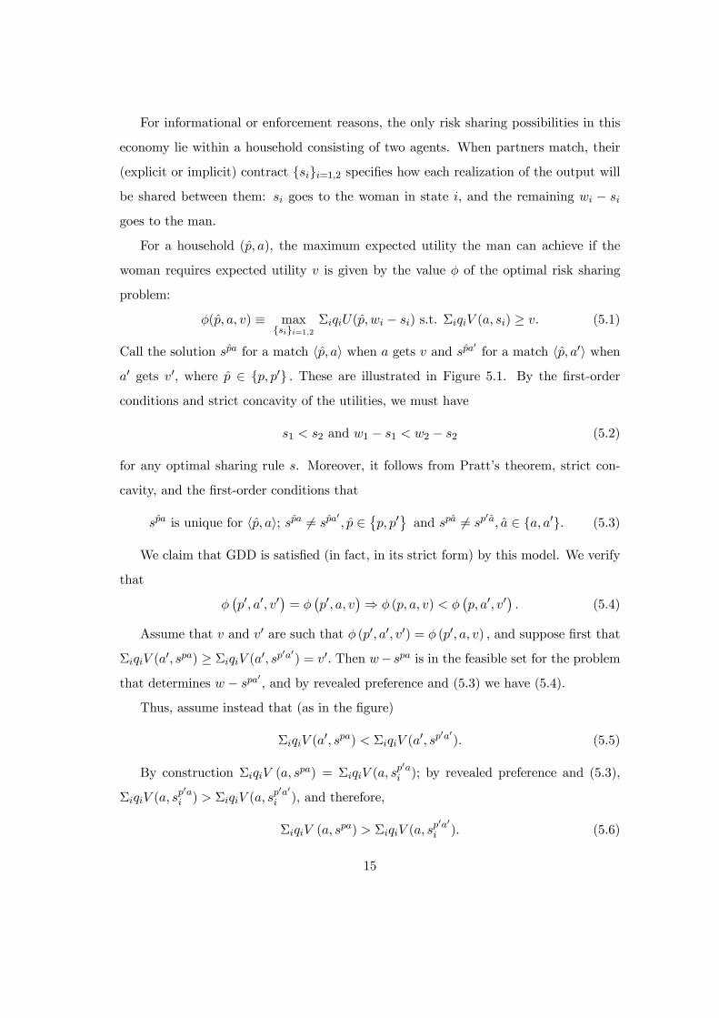
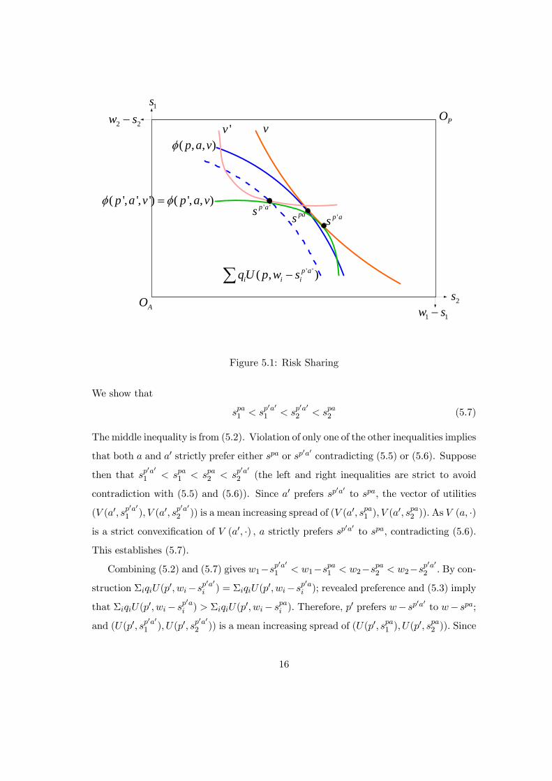
φ(p, a, v) ≡ maxsii=1,2
ΣiqiU(p, wi − si) s.t. ΣiqiV (a, si) ≥ v. (5.1)
Call the solution spa for a match hp, ai when a gets v and spa0for a match hp, a0i when
a0 gets v0, where p ∈ p, p0 . These are illustrated in Figure 5.1. By the first-order
conditions and strict concavity of the utilities, we must have
s1 < s2 and w1 − s1 < w2 − s2 (5.2)
for any optimal sharing rule s. Moreover, it follows from Pratt’s theorem, strict con-
cavity, and the first-order conditions that
spa is unique for hp, ai; spa 6= spa0, p ∈
©p, p0
ªand spa 6= sp
0a, a ∈ a, a0. (5.3)
We claim that GDD is satisfied (in fact, in its strict form) by this model. We verify
that
φ¡p0, a0, v0
¢= φ
¡p0, a, v
¢⇒ φ (p, a, v) < φ
¡p, a0, v0
¢. (5.4)
Assume that v and v0 are such that φ (p0, a0, v0) = φ (p0, a, v) , and suppose first that
ΣiqiV (a0, spa) ≥ ΣiqiV (a0, sp
0a0) = v0. Then w− spa is in the feasible set for the problem
that determines w − spa0, and by revealed preference and (5.3) we have (5.4).
Thus, assume instead that (as in the figure)
ΣiqiV (a0, spa) < ΣiqiV (a
0, sp0a0). (5.5)
By construction ΣiqiV (a, spa) = ΣiqiV (a, sp0ai ); by revealed preference and (5.3),
ΣiqiV (a, sp0ai ) > ΣiqiV (a, s
p0a0
i ), and therefore,
ΣiqiV (a, spa) > ΣiqiV (a, s
p0a0
i ). (5.6)
15
'p as' 'p as pas
v'v2 2w s−
1 1w s−2s
1s
AO
PO
( , , )p a vφ
( ', ', ') ( ', , )p a v p a vφ φ=
' '( , )p ai i iqU p w s−∑
Figure 5.1: Risk Sharing
We show that
spa1 < sp0a0
1 < sp0a0
2 < spa2 (5.7)
The middle inequality is from (5.2). Violation of only one of the other inequalities implies
that both a and a0 strictly prefer either spa or sp0a0 contradicting (5.5) or (5.6). Suppose
then that sp0a0
1 < spa1 < spa2 < sp0a0
2 (the left and right inequalities are strict to avoid
contradiction with (5.5) and (5.6)). Since a0 prefers sp0a0 to spa, the vector of utilities
(V (a0, sp0a0
1 ), V (a0, sp0a0
2 )) is a mean increasing spread of (V (a0, spa1 ), V (a0, spa2 )). As V (a, ·)
is a strict convexification of V (a0, ·) , a strictly prefers sp0a0 to spa, contradicting (5.6).
This establishes (5.7).
Combining (5.2) and (5.7) gives w1−sp0a0
1 < w1−spa1 < w2−spa2 < w2−sp0a0
2 . By con-
struction ΣiqiU(p0, wi−sp0a0
i ) = ΣiqiU(p0, wi−sp
0ai ); revealed preference and (5.3) imply
that ΣiqiU(p0, wi− sp0ai ) > ΣiqiU(p
0, wi− spai ). Therefore, p0 prefers w− sp
0a0 to w− spa;
and (U(p0, sp0a0
1 ), U(p0, sp0a0
2 )) is a mean increasing spread of (U(p0, spa1 ), U(p0, spa2 )). Since
16

U (p, ·) is a strict convexification of U (p0, ·) , p strictly strictly prefers w−sp0a0 to w−spa,
or ΣiqiU(p,wi−sp0a0
i ) > ΣiqiU(p,wi−spai ) = φ (p, a, v) . Finally, by revealed preference,
φ (p, a0, v0) ≥ ΣiqiU(p,wi − sp0a0
i ) and therefore φ (p, a0, v0) > φ (p, a, v) proving (5.4).
Thus strict GDD is satisfied, and we conclude that in the risk-sharing economy men
and women will always match negatively in risk attitude. This is intuitive: a risk-neutral
agent is willing to offer a better deal for insurance than is a risk averse one, so those
demanding the most insurance (the most risk averse) will share risk with the least risk
averse, while the moderately risk averse share with each other.8
In case the frontier φ admits a closed form solution, verification of the GDC is
straightforward. For instance, putting U(p, y) = log(1+ p+ y), V (a, y) = log(1+ a+ y)
(type represents initial wealth, which may be shared within the partnership; the number
of income realizations can be arbitrary), one obtains φ(p, a, v) = log(1− ev−Σpa) +Σpa,
where Σpa denotes Σiqi log(wi + p+ a+ 2). Then
φ(p, a, ψ(a, p0, v) = log(1− eΣp0a−Σpa + ev−Σpa) + Σpa
and
φ(p, a0, ψ(a0, p0, v) = log(1− eΣp0a0−Σpa0 + ev−Σpa0 ) + Σpa0 .
Now,
φ(p, a, φ(a, p0, v)) < φ(p, a0, φ(a0, p0, v))
if and only if
(1− eΣp0a−Σpa + ev−Σpa)eΣpa < (1− eΣp0a0−Σpa0 + ev−Σpa0 )eΣpa0 ,
that is if eΣpa − eΣp0a < eΣpa0 − eΣp0a0 . This is just the requirement that the func-
tion eΣpa satisfies strict decreasing differences, which it clearly does, since ∂2
∂p∂aeΣpa =
−eΣpaV ar( 1w+p+a+2) < 0.
For this logarithmic case, the local condition (4.4) does not apply: it is easy to check
that φ1, φ2 > 0 and φ12 < 0, while φ13 > 0. However, the model in the next subsection
does admit application of the local conditions.
8Recently, Chiappori and Reny (2006) have extended this argument to show that strict GDD holds
in the case of an arbitrary number of states.
17
5.2. Matching Principals and Agents
Principals’ projects have a common expected return but differ in their risk characteris-
tics; they must match with agents, who differ in initial wealth. Agents have declining
absolute risk aversion, and the question is whether the safest projects are tended by the
most or the least risk averse, i.e., the poorest or wealthiest agents.
Risk-neutral principals have type indexed by p ∈ [p, 1], and agents have type index
a ∈ [a, a], where p, a > 0. Agents’ unobservable effort e can either be 1 or 0. The
principal’s type indexes the success yield and probability of his project: it yields R/p
with probability p and 0 with probability 1 − p provided his agent exerts e = 1; it
yields 0 with probability 1 if e = 0. Thus, conditional on high effort, all tasks have the
same expected return R, but higher p implies lower risk. An agent of type a has utility
V (a+ y) from income y; her type represents initial wealth. V (·) is twice differentiable
and unbounded below, V 0 > 0 > V 00, and it displays increasing absolute risk tolerance.
The frontier for a principal of type p who is matched to an agent of type a is given
by
φ(p, a, v) = maxs0,s1
R− ps1 − (1− p)s0
s.t. pV (a+ s1) + (1− p)V (a+ s0)− 1 ≥ V (a+ s0),
pV (a+ s1) + (1− p)V (a+ s0)− 1 ≥ v
where s1 and s0 are the wages paid in case of success and failure respectively.9 The
first inequality is the incentive compatibility condition that ensures the agent takes high
effort.
Intuition might suggest that since wealthier agents are less risk averse, they should be
matched to riskier tasks while the more risk averse agents should accept the safer tasks
(i.e., there should be NAM in (p, a)).
9 In this example, the agents’ autarchy payoffs are not zero, at least if it assumed that they can
consume their initial wealth. As we note in Section 7.1, this generalization presents no particular
difficulty.
18

But this intuition is incomplete, and indeed misleading, as the following application
of Corollary 1 shows. By standard arguments, both constraints bind. Let C(·) ≡ V −1(·).
Thus V (a+ s1) =1p+ V (a+ s0), and V (a+ s0) = v, from which
φ(p, a, v) = R+ a− pC(1
p+ v)− (1− p)C(v).
Thus,
φ1(p, a, v) =1
pC 0(
1
p+ v)− C(
1
p+ v) + C(v)
φ2(p, a, v) = 1,
φ12 = 0,
φ13(p, a, v) =1
pC 00(
1
p+ v)− C 0(
1
p+ v) +C 0(v).
φ1 is positive since C00 > 0, so φ is type increasing. Notice that if C 0 is convex (equiva-
lently V 00/V 03 is decreasing; see Jewitt, 1988 for a discussion — all utilities of the CRRA
class that are more risk averse than square root utility have this property), then φ13 ≥ 0 :
there is PAM in (p, a) : as long as risk aversion does not decline “too quickly,” agents
with lower risk aversion (higher wealth) are matched to principals with projects that are
safer, i.e., more likely to succeed. This result may appear surprising, since empirically
we tend to associate (financially) riskier tasks to wealthier workers.10
The explanation is that in the standard version of the principal-agent model with
utility additively separable in income and effort, incentive compatibility for a given effort
level entails that the amount of risk borne by the agent increases with wealth (ds1ds0> 0
along the incentive compatibility constraint). This effect arises from the diminishing
marginal utility of income. Though wealthier agents tolerate risk better than the poor,
they must accept more risk on a given task; with C 0 convex, the latter effect dominates,
and the wealthy therefore prefer the safer tasks. Put another way, a less risky task
allows for a reduction in risk borne by the agent; given the increasing risk effect of
incentive compatibility, the benefit of the risk reduction is greater for the rich than for
the poor, and this generates a complementarity between safety and wealth.
10Of course, if risk aversion declines fast enough — C0 is concave — then the “intuitive” negative
matching pattern obtains, though this entails a possibly implausibly high level of risk tolerance.
19
The result offers a possible explanation for the finding in Ackerberg and Botticini
(2002) that in medieval Tuscany, wealthy peasants were more likely than poor peasants
to tend safe crops (cereals) rather than risky ones (vines).
This example is instructive because the entire effect comes from the nontransfer-
ability of the problem. There is no direct “productive” interaction between principal
type and agent type (φ12 = 0); only the type-payoff complementarity plays a role in
determining the match.
6. Ordinality, Necessity, Modularity
In this section we investigate the strength of the GDC. First, we note that GID and GDD
are preserved under ordinal transformations of types’ preferences. This implies that the
analyst is free to choose whichever representation of preferences is most convenient, and
leads to a weakening of the differential conditions. In a number of cases, the NTU
model even admits a TU representation, in which case GID and GDD reduce to ID and
DD of the joint payoff function induced by the representation. After a brief discussion
of necessity, we turn to a comparison of the GDC with well-known lattice theoretic
concepts.
6.1. Ordinality
The core of an economy, and thus any core matching pattern, is independent of the
cardinal representation of preferences. However, some representations may be easier to
work with after monotone transformations of types’ utilities; in some instances it may
be possible to recover a transferable utility representation.
Let F (u; p) be a strictly increasing transformation applied to type p’s utility u and
let F−1 (u; p) be its inverse. Similarly, transform type a’s utility by G(v; a). Let
φF,G (p, a, v) = F (φ(p, a,G−1(v; a)); p),
be the new frontier functions after transformations F and G are applied. We call φF,G a
representation of φ. Its quasi-inverse is ψG,F (a, p, u) = G¡ψ¡a, p, F−1 (u; p)
¢; a¢. The
20
following result, proved in the Appendix, shows the invariance of the GID condition to
ordinal transformations of agents’ utilities.
Proposition 2. Suppose GID holds for φ. Then GID holds for any other frontier func-
tion generated from φ by increasing transformations of types’ utilities. The same result
is true for GDD.
A suitably chosen representation of φ may be easier to work with than φ itself. In
particular, though the generalized difference conditions are preserved for all representa-
tions of φ, not so the differential conditions in Corollary 1. Hence, while the differential
conditions may not hold for φ, they might hold for an alternate representation φF,G.
It is enough that one representation of φ satisfy condition (4.3) or (4.4) to guarantee
monotone matching.
For instance, in the logarithmic version of risk sharing in Section 5.1, transform the
utility by exponentiation for all types, i.e., set F (v; p) = ev and G(u; a) = eu; then
φF,G(p, a, v) = eΣpa−v. Unlike φ, which does not satisfy the conditions in Corollary 4.3,
φF,G does, since φF,G12 < 0 = φF,G13 . Notice that the transformation of payoffs actually
yields an expression of the frontiers in a transferable utility form.
Starting with a model φ(p, a, v), say that it is TU-representable if there is a repre-
sentation φF,G of φ and a function h(p, a) such that
∀p, a, v, F (φ(p, a, v); p) = h(p, a)−G(v; a). (6.1)
Then F (φ(p, a, v); p) is a TU model, since the transformed payoffs to p and to a sum
to h(p, a), independently of the distribution of transformed utility between p and a. A
consequence of Proposition 2 is that φ satisfies GID if and only if h satisfies increasing
differences.
Corollary 2. Suppose that φ has a TU representation φF,G. Then φ satisfies GID
(GDD) if and only if h satisfies ID (DD), where h is defined in (6.1).
A well-known-example of a model that admits a TU representation is the “linear-
normal-exponential” version of the Principal-Agent model (Holmström and Milgrom,
21
1987) in which a TU representation is found by looking at players’ certainty equivalent
incomes rather than their expected utilities.11
6.2. Necessity
It should come as little surprise — and for completeness is established in the Appendix
— that given a frontier function, if every distribution of types gives rise to an economy
that satisfies PAM, that frontier function must satisfy GID.
Proposition 3. If the equilibrium outcome is payoff equivalent to PAM (NAM) for
every distribution of types, then the frontier function φ satisfies GID (GDD).
In other words, if GID is not satisfied, there are type distributions for which the
matching pattern will not be payoff equivalent to PAM.12 If GDD isn’t satisfied either,
then matching need not be monotone. In some cases, matching will be positive assorta-
tive for some type distributions, negative assortative for others, and nonmonotone for
others still. See Legros and Newman (2002a) for examples.
6.3. Comparison with Lattice Theoretic Conditions
In TU models, supermodularity of φ (p, a, v) is equivalent to increasing differences of
the production function h(p, a), hence to GID.13 It is natural to ask whether there is a
relationship of GID to supermodularity for NTU models.
11See for instance Wright (2004) and Serfes (2005) for recent applications to matching. Our principal-
agent example also has a TU representation if agents’ income utility is taken to be logarithmic.
12Notice this necessity result does not say that the GID condition must hold if a particular economy
has an equilibrium that is (payoff equivalent to) a positively assortative one: the GID inequality need
only hold for the types in the support of that economy’s distribution and for the equilibrium payoff
levels. Of course, in case φ has a TU representation, then GID is also necessary for PAM in this
stronger sense. It is an open question whether the family of frontiers such that GID is necessary for
PAM is broader than the class of TU representable models.
13A function f (x) defined on a lattice L is supermodular when x, y ∈ L implies f (x ∧ y)+f (x ∨ y) ≥
f (x) + f (y) . Here, L ⊂ Rn, and x ∧ y (x ∨ y) denote the componentwise minimum (maximum) of x
and y.
22
It is evident from Corollary 1 that a sufficient condition for GID is that φ is type
increasing and supermodular in (p, a) and in (p, v). The principal interest of this obser-
vation is that it enables us to offer sufficient conditions for monotone matching expressed
in terms of the fundamentals of the model, rather than in terms of the frontiers. Recall-
ing the notation in footnote 5, let U(x, p, a) be the utility function of choice variables x
for type-p principal matched to a type-a agent, V (x, a, p) be the corresponding agent’s
utility, Ω(a, p) their choice set, and Λ(a, p, v) = x : V (x, a, p) ≥ v.
A simple application of Theorem 2.7.6 of Topkis (1998) tells us that a sufficient
condition for φ to be type increasing and super- (sub-) modular in (p, a) and (p, v) and
therefore for GID (GDD) is that U is super- (sub-) modular and nondecreasing in (p, a) ,
V is nondecreasing in (a, p) and that the set
Sv = (p, a, x) : x ∈ Ω(a, b) ∩ Λ(a, p, v)
is a sublattice for each v and the set
Sa = (p, a, x) : x ∈ Ω(a, b) ∩ Λ(a, p, v)
a sublattice for each a.
Practically speaking, verification/satisfaction of the sublattice property may be dif-
ficult. In the case of logarithmic risk sharing of section 5.1, Sa is not a sublattice since
U is submodular while φ is supermodular in (p, v). The monotonicity requirements are
also strong: in the principal agent example of section 5.2, the objective is not increasing
in p, though the frontier is. In any case, supermodularity is clearly stronger than GID.
Are there weaker known conditions on frontier that suffice for assortative matching?
One such a concept is quasi-supermodularity (QSM), which requires of a function f
defined on a lattice L that for any x, y ∈ L,
f (x) ≥ f (x ∧ y)⇒ f (x ∨ y) ≥ f (y) , (6.2)
with strict inequality on the left-hand side implying strict inequality on the right-hand
side (Milgrom and Shannon, 1994). Like GID, QSM is a kind of single-crossing condition
on products of lattices.
23

It is easily verified that quasi-supermodularity (QSM) in (p, a) and in (p, v) is
satisfied for all frontiers φ that satisfy (strict) type-monotonicity. Since strict type-
monotonicity is not sufficient for GID (in particular, for TU models, monotonicity of
the output function is well-known to be insufficient for PAM; the example in section 2
is a case in point), quasi-supermodularity in (p, a) and in (p, v) is not sufficient for GID,
unlike supermodularity in (p, a) and in (p, v) .
Nevertheless, when we assume that φ (p, a, v) is nondecreasing in a, quasi-supermodularity
of φ in (p, a, v) implies GID. The two concepts do not coincide, however, as we show
in two examples in the Appendix: Example 1 shows that there exist frontiers that are
type increasing for which GID holds but not QSM; Example 2 shows that when φ is
decreasing in a, there are frontiers satisfying QSM but neither GID nor GDD.
Proposition 4. Consider the set of maps φ : P × A × R+ → R+, strictly decreasing
in the third argument. If φ is nondecreasing in its second argument, then QSM of φ
implies GID.
7. Extensions
7.1. Type-Dependent Autarchy Payoffs and Uneven Sides
Suppose that autarchy generates a payoff u(p) to type p and v (a) to type a; if u(·) and
v (·) are continuous, we can assume without loss of generality that u(·) ≥ 0, v (·) ≥ 0.
Then all the propositions go through as before, since if the generalized difference or
differential conditions hold for nonnegative payoffs, they hold on the restricted domain
of individually rational ones. Equilibrium will now typically entail that some types
remain unmatched, but among those matched, the pattern will be monotone if the
appropriate difference condition holds.
By the same token, little changes if the cardinality of the two sides differs. Some
agents on the long side will be left out of the match, but the GID condition implies that
those who are matched will be positively assorted: our main result implies that those
who are matched initially can be rearranged if necessary in a positive assortative fashion
24

while receiving the same payoffs. The unmatched agents, who before were unable to
underbid any matched agent, will still be unable to do so.
7.2. One-Sided Models
One sided models, in which the type space is just A, introduce two complications. First
they admit a richer variety of monotone matching patterns than two-sided models.14.
Second, as is well known, they may have existence problems, at least in finite economies.
Nevertheless, the apparatus developed here can be adapted straightforwardly to the one-
sided case to characterize equilibria when they exist.
Now GID takes the form φ (a0, a, φ (a, a00, v)) increasing in a for all v ≤ φ (a00, a, 0) , a0 >
a00 (note that ψ (a, a0, v) = φ (a, a0, v)). If GID holds, we obtain a special form of PAM:
segregation, wherein matched pairs consist of identical agents (obviously, this requires
an even number of agents of each type). The proof mimics that of Proposition 1 in
showing that any heterogenous match is unstable if GID holds. Sufficiency of GDD for
NAM is shown similarly; we refer the reader to our working paper (Legros and Newman
2002b).
7.3. Strict NTU
Our model excludes the extreme case in which the Pareto frontier for a matched pair is a
point, as in the literature surveyed in Roth and Sotomayor (1990). Becker (1973) shows
that strict monotonicity of the payoffs in type is sufficient for assortative matching in
this case. It turns out that while the strict NTU model can be obtained as a limit
case of ours, there are discontinuities in the limit. For instance, GID can be satisfied
by an economy with strict NTU but not by nearby economies with strictly decreasing
frontiers. GID still implies the existence of a PAM equilibrium, but there may also
be other equilibria that are not payoff equivalent to a PAM equilibrium. However, if
agents are never indifferent between partners, GID is sufficient for an economy to satisfy
14 In the one-sided model, matching satisfies PAM (NAM) if for any two matched pairs ha, a0i and
ha, a0i, maxa, a0 > maxa, a0 =⇒ mina, a0 ≥ (≤)mina, a0.
25

PAM, which weakens Becker’s condition. See Legros and Newman (2006a), which also
shows that GID is a strengthening of Clark’s (2006) and Eeckout’s (2000) conditions
for uniqueness of equilibrium.
7.4. Continuum Economies
Since the GDC conditions are distribution free, our restriction to a finite number of
agents is without much loss of generality. When the GID condition is strict, then even
in economies with a continuum of agents and/or types, there can never be a negative
stable match and PAM is the only equilibrium outcome. When the GID condition holds
weakly, then whenever an equilibrium exists, it is possible to construct an equilibrium
that is positive assortative. However, to establish the stronger analog of Proposition 1,
that is, that any equilibrium is payoff equivalent to an equilibrium satisfying PAM, the
algorithm used in the proof of Proposition 1 for finite economies is not applicable and
has to be replaced by a limit argument. See Legros and Newman (2006b).
8. Conclusion
Many economic situations involving nontransferable utility are naturally modeled as
matching or assignment games. We have presented some general sufficient conditions
for monotone matching in these models. These have an intuitive basis and appear to be
reasonably straightforward to apply. Specifically, if one wants to ensure PAM, it does
not suffice only to have complementarity in types; one must ensure as well that there is
enough type-payoff complementarity.
Implicitly motivating this paper’s focus on properties of the economic environment
that lead to monotone matching is the question of how changes in that environment
affect matching patterns. Space, not to mention the present state of knowledge, is too
limited to offer a complete answer to this question here, but being able to go beyond the
TU case is a necessary part of the puzzle. Many phenomena that could be characterized
as mass re-assignments of partners can be understood as manifestations of changes to
the degree of transferability.
26

For instance, mergers and divestitures involve reassignments of say, upstream and
downstream divisions of firms. Transferability between divisions depends in part on
the efficiency of financial markets, with the magnitude of the effect dependent on char-
acteristics of individual firms such as liquidity position or productivity. Deregulations
or innovations in financial markets will typically alter transferability and may lead to
widespread reassignment of partnerships between upstream and downstream divisions,
i.e., “waves” of corporate reorganization (Holmström and Kaplan, 2001).
Another example is a policy like Title IX, which requires US schools and universities
receiving federal funding to spend equally on men’s and women’s activities (athletic
programs having garnered the most public attention), or suffer penalties in the form
of lost funding. If one models a college as partnership between a male and female
student-athlete, identifying their types with the revenue-generating capacities of their
respective sports, the policy acts to transform a TU model into an NTU one, rather
like the example of section 2. Imposing Title IX would lead to a reshuffling of the types
of males and females who match; the male wrestler (low revenue), formerly matched
to the female point guard (high revenue), will now match with, say, a female rower,
while the point guard now plays at a football school. There is evidence that this sort
of re-assignment has taken place: the oft-noted terminations and contractions of some
sports at some colleges are ameliorated by start-ups and expansions at others.
9. Appendix
9.1. Proof of Proposition 1
We prove (1), the proof of (2) is similar. The proof has two steps. We first establish
that when GID holds, any equilibrium matching four types in a NAM fashion has the
property that we can rematch these types in a PAM fashion without violating feasibility.
We then show that if an equilibrium does not satisfy PAM we can use recursively the
previous result to construct a type payoff equivalent equilibrium that satisfies PAM.
Lemma 1. Suppose that GID holds. Consider an equilibrium and associated stable
27
hM, π, ωi. If a0 ∈M (p) , a ∈M (p0), where a > a0 and p > p0, then π (p) = φ (p, a, ω (a)) ,
ω (a) ≤ ψ (a, p, 0) and π (p0) = φ (p0, a0, ω (a0)) and ω (a0) ≤ ψ (a0, p0, 0) .
Proof. Consider a NAM matching as in the Lemma with payoffs π and ω. Feasibility
entails
π (p) = φ¡p, a0, ω
¡a0¢¢and ω
¡a0¢≤ ψ
¡a0, p, 0
¢(9.1)
π¡p0¢= φ
¡p0, a, ω (a)
¢and ω (a) ≤ ψ
¡a, p0, 0
¢(9.2)
Stability of the NAM matching requires
ω¡a0¢≥ ψ
¡a0, p0, π
¡p0¢¢
(9.3)
π (p) ≥ φ (p, a, ω (a)) . (9.4)
From (9.4) and (9.2),
π (p) ≥ φ (p, a, ω (a)) = φ¡p, a, ψ
¡a, p0, π
¡p0¢¢¢
(9.5)
From (9.2), π (p0) ≤ φ (p0, a, 0) and by GID,
φ¡p, a, ψ
¡a, p0, π
¡p0¢¢¢≥ φ
¡p, a0, ψ
¡a0, p0, π
¡p0¢¢¢
. (9.6)
From (9.3) and (9.1),
φ¡p, a0, ψ
¡a0, p0, π
¡p0¢¢¢≥ φ
¡p, a0, ω
¡a0¢¢= π (p) (9.7)
Hence, from (9.5)-(9.7), we must have an equality everywhere, or
π (p) = φ (p, a, ω (a)) = φ¡p, a0, ψ
¡a0, p0, π
¡p0¢¢¢
= φ¡p, a0, ω
¡a0¢¢= π (p) . (9.8)
Case 1: π (p) > 0. In (9.8), π (p) = φ (p, a, ω (a)) shows that (π (p) , ω (a)) is feasible
for (p, a) ; since φ (p, a0, ψ (a0, p0, π (p0))) > 0, it follows that ψ (a0, p0, π (p0)) = ω (a0) ≤
ψ (p, a0, 0) and therefore (π (p0) , ω (a0)) is feasible for (p0, a0) .
Case 2: π (p) = 0. Then ω (a0) = ψ(a0, p, 0) > 0, and by stability, ω (a) ≥ ψ (a, p, 0) .
We show that we cannot have ω (a) > ψ (a, p, 0) . If we do, define u0 = φ(p0, a, ψ(a, p, 0)).
Then φ(p0, a, 0) > u0 > φ(p0, a, ω(a)) = π(p0). By construction, φ(p, a, ψ(a, p0, u0))) = 0.
28

If u0 ≤ φ(p0, a0, 0), then ψ(a0, p0, u0) < ψ(a0, p0, π (p0)) ≤ ω(a0) by (9.3); if u0 > φ(p0, a0, 0)
then ψ(a0, p0, u0) = 0 < ω(a0). Thus φ(p, a0, ψ(a0, p0, u0)) > φ(p, a0, ω (a0)) = π (p) = 0 =
φ(p, a, ψ(a, p0, u0))), and we have a contradiction of GID.
Therefore ω (a) = ψ (a, p, 0) and (0, ω (a)) is feasible for (p, a) . From (9.8), φ (p, a0, ψ (a0, p0, π (p0))) =
0, so ψ (a0, p0, π (p0)) ≥ ψ(a0, p, 0) = ω (a0) . But by stability (9.3) we must have an equal-
ity: ψ (a0, p0, π (p0)) = ω (a0), i.e., (π (p0) , ω (a0)) is feasible for (p0, a0) .
We have shown that under GID, if in equilibrium there are two matches that violate
PAM, it is possible to reassign partners in order to obtain PAM without modifying
payoffs and therefore without violating stability. This falls short, however, of showing
that starting from an equilibrium in whichM does not satisfy PAM we can find a payoff
equivalent equilibrium satisfying PAM.
The next part of the proof shows an algorithm to construct a new equilibrium
hM0, π, ωi whereM0 satisfies PAM and π and ω are the initial equilibrium type payoffs.
It is easier to develop the argument in reference to agents rather than types. Let N be
the cardinalities of I and J . Then, we can write I = ik, k ∈ 1, 2, . . . , N and J =
jk, k ∈ 1, 2, . . . , N . Higher indexes correspond to lower values of the characteristic,
that is agent ik has type p and agent il has type p0 where p ≥ p0 if and only if k ≤ l.
We show that under GID, any equilibrium hm,π∗, ω∗i is payoff equivalent to the
equilibrium hm∗, π∗, ω∗i with m∗ (ik) = jk.
Suppose that in hm,π∗, ω∗i , m (ik) = jl, l 6= k. Let k0 be the first time this situation
arises. Hence for all t ≤ k0 − 1, m(it) = m∗ (it) = jt. Let ir be such that m (ir) = jk0 ;
by construction if ik0 has type p and jk0 has type a, jl has type a0 ≤ a and ir has type
p0 ≤ p. By the Lemma, we can match ik0 with jk0 and ir with jl, keep the same payoffs
for the four agents without violating feasibility or stability. Doing so we have a new
matching m[1]
m[1] (it) =
⎧⎪⎪⎪⎨⎪⎪⎪⎩m∗(it) if t ≤ k0
m (it) if t ≥ k0 + 1, t 6= r
jl if t = r.
29
Ifm[1] = m∗, we are done. Otherwise, let k1 be the first index such thatm[1] (it) 6= jt;
by construction of m[1], it must be the case that k1 ≥ k0 + 1. Repeat the previous
construction to obtain a new matching function m[2] with m[2] (t) = m∗ (t) for t ≤ k1.
Repeating this construction, we will have a value n such that m[n] = m∗. Stability of
m∗ with respect to (π∗, ω∗) is inherited from the stability of m with respect to (π∗,m∗).
Hence hm∗, π∗, ω∗i is an equilibrium satisfying PAM, concluding the proof.
9.2. Proof of Corollary 1
Consider a > a0, p > p0 and u ≤ φ (p0, a, 0) . By type monotonicity φ (p0, a, 0) ≥
φ (p0, a0, 0) .
If u ∈ [φ (p0, a0, 0) , φ (p0, a, 0)] , φ (p, a, ψ (a, p0, u)) = φ (p, a, 0) which is greater than
φ (p, a0, 0) by type monotonicity. Hence, φ (p, a, ψ (a, p0, u)) ≥ φ (p, a0, ψ (a0, p0, u)) .
If u ∈ (0, φ (p0, a0, 0)) , since φ is type monotonic, when a ≥ a0, and p ≥ p0,
φ (p0, a0, 0) ≤ φ (p, a, 0) , therefore u < φ (p, a, 0) . Letting v = ψ (a0, p0, u) , (p, a, v) ∈ D
and φ12 (p, a, v) is well defined for all a ≥ a0 and p ≥ p0. Therefore,
0 ≤Z a
a0φ12 (p, a, v) da (9.9)
= φ1 (p, a, v)− φ1¡p, a0, v
¢.
Since φ13 ≥ 0, we have for all p ≥ p0, φ1 (p, a, ψ (a, p0, u)) ≥ φ1 (p, a, ψ (a
0, p0, u)) which
together with (9.9) leads to
φ1¡p, a, ψ
¡a, p0, u
¢¢≥ φ1
¡p, a0, ψ
¡a0, p0, u
¢¢. (9.10)
Integrating both sides with respect to p on the interval [p0, p] leads to
φ¡p, a, ψ
¡a, p0, u
¢¢− φ
¡p0, a, ψ
¡a, p0, u
¢¢≥ φ
¡p, a0, ψ
¡a0, p0, u
¢¢− φ
¡p0, a0, ψ
¡a, p0, u
¢¢.
Since φ (p0, a, ψ (a, p0, u)) and φ (p0, a0, ψ (a, p0, u)) are both equal to u, we obtain the
GID condition.
If u = 0, consider a sequence uk ⊂ (0, φ (p0, a0, 0)) converging to 0. For each k, we
have by the previous case φ (p, a, ψ (a, p0, uk)) ≥ φ (p, a0, ψ (a0, p0, uk)) ; since φ and ψ are
continuous, taking the limit on both sides with respect to k yields φ (p, a, ψ (a, p0, 0)) ≥
φ (p, a0, ψ (a0, p0, 0)) .
30
9.3. Proof of Claim in Remark 1
Suppose GID and let u ∈ (0, φ (p0, a, 0)) . Since (p0, a, ψ (a, p0, u)) ∈ D, type monotonicity
implies that for all p > p0, (p, a, ψ (a, p0, u)) ∈ D. If GID holds, φ (p, a, ψ (a, p0, u)) is
nondecreasing in a for p > p0; since this function is differentiable in a, we must have
0 ≤ ddaφ (p, a, ψ (a, p
0, u)) = φ2(p, a, ψ (a, p0, u)) + φ3(p, a, ψ (a, p
0, u)) · ψ1(a, p0, u). This
proves necessity.
For sufficiency, consider a0 < a, p0 < p and u ≤ φ (p0, a, 0) . If u ∈ [φ (p0, a0, 0) , φ (p0, a, 0)] ,
GID holds since φ (p, a, ψ (a, p0, u)) = φ (p, a, 0) . If u ∈ (0, φ (p0, a0, 0)) , since φ is type
increasing, for all a ≥ a, ψ (a, p0, u) ≤ ψ (a, p, u) and therefore, (p, a, ψ (a, p0, u)) ∈ D,
which shows that φ (p, a, ψ (a, p0, u)) is differentiable with respect to a. Hence, integrat-
ing (4.5) on [a0, a] leads to the GID condition. If u = 0, use a limit argument as in the
previous proof.
9.4. Proof of Proposition 2
We consider the case for GID; the proof for GDD is similar. It is enough to show that
the map φF,G (p, a, v) satisfies GID, that is that φF,G¡p, a, ψG,F (a, p0, u)
¢is increasing
in a.
φF,G¡p, a, ψG,F
¡a, p0, u
¢¢= F (φ(p, a,G−1(ψG,F
¡a, p0, u
¢; a); p)
= F¡φ(p, a,G−1(G
¡ψ¡a, p0, F−1
¡u; p0
¢¢; a¢; a); p
¢= F
¡φ(p, a, ψ
¡a, p0, F−1
¡u; p0
¢¢; p¢,
since F (·; p) is strictly increasing, φF,G¡p, a, ψG,F (a, p0, u)
¢is increasing in a only if
φ(p, a, ψ¡a, p0, F−1 (u; p0)
¢is increasing in a, which is true since φ satisfies GID.
9.5. Proof of Proposition 3
Consider PAM, as the case for the necessity of GDD for NAM is similar. Suppose there
are p, p0 ∈ P, p > p0 and a, a0 ∈ A, a > a0, and a payoff level u ≤ φ (p0, a, 0) such that
φ(p, a, ψ(a, p0, u)) < φ(p, a0, ψ(a0, p0, u)). Then we can find a distribution of types such
that there is an equilibrium that is not payoff equivalent to PAM.
31

To see this, put an equal number of agents at each of the four types p, p0, a, a0.
Then there is > 0 such that hp0, ai with payoffs (u, ψ(a, p0, u)) and hp, a0i with payoffs
(φ(p, a0, ψ(a0, p0, u)+ ), ψ(a0, p0, u)+ )) is an equilibrium. To verify stability, note that by
continuity of φ in v, for small enough, φ(p, a, ψ(a, p0, u)) < φ(p, a0, ψ(a0, p0, u)+ ). Thus
p would be strictly worse off switching to a as long as a receives at least his equilibrium
payoff. Similarly a0 would lose by switching to p0. Finally, the match is not payoff
equivalent to PAM because p cannot generate φ(p, a0, ψ(a0, p0, u) + ) in a match with
a without offering a less than ψ(a, p0, u) And no match with PAM could support these
payoffs, since the same inequality implies that p cannot generate his equilibrium payoff
in a match with a.
9.6. Proof of Proposition 4
Let p > p0, a > a0. We establish GID, i.e.,
φ¡p0, a0, v0
¢= φ
¡p0, a, v
¢⇒ φ (p, a, v) ≥ φ
¡p, a0, v0
¢(9.11)
Suppose φ (p0, a0, v0) = φ (p0, a, v) ; since φ is nondecreasing in its second argument and
decreasing in its third, we have v ≥ v0. Put x = (p0, a, v) and y = (p, a0, v0) ; then
x ∧ y = (p0, a0, v0) and x ∨ y = (p, a, v) . We therefore have φ(x) = φ (x ∧ y) , and by
QSM, φ(x ∨ y) ≥ φ(y), i.e., φ (p, a, v) ≥ φ (p, a0, v0) , as desired.
9.7. QSM and the GDC
Example 1.
The example shows that within the set of type increasing frontiers, QSM is a
stronger concept than GID. The construction resembles that in section 2: starting from
a pair of payoffs f (p|a) to p and g(a|p) to a, that serves as a “reference point” for a
match (p, a) , construct a frontier φ (p, a, v) by allowing transfers at a rate β away from
the reference payoff. Consider p > p0, a > a0, with the reference points for the four
32
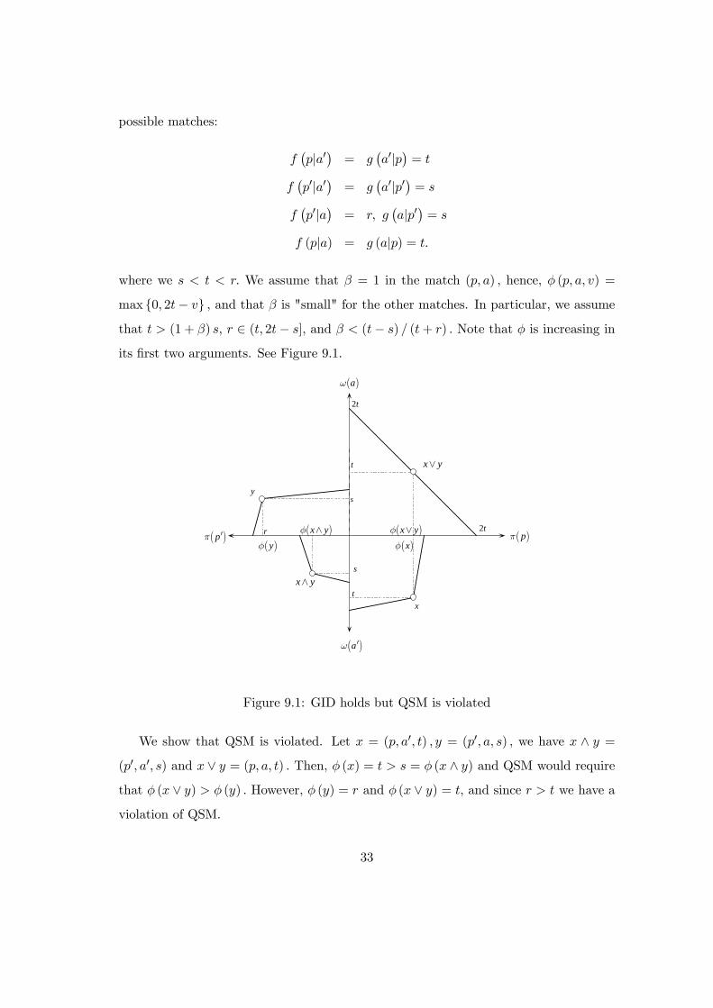
possible matches:
f¡p|a0
¢= g
¡a0|p
¢= t
f¡p0|a0
¢= g
¡a0|p0
¢= s
f¡p0|a
¢= r, g
¡a|p0
¢= s
f (p|a) = g (a|p) = t.
where we s < t < r. We assume that β = 1 in the match (p, a) , hence, φ (p, a, v) =
max 0, 2t− v , and that β is "small" for the other matches. In particular, we assume
that t > (1 + β) s, r ∈ (t, 2t− s], and β < (t− s) / (t+ r) . Note that φ is increasing in
its first two arguments. See Figure 9.1.
2t
2t
t
t
s
r
s
x
( )yφ ( )xφ
y
x y∧
x y∨
( )x yφ ∧ ( )x yφ ∨ ( )pπ
( )aω ′
( )aω
( )pπ ′
Figure 9.1: GID holds but QSM is violated
We show that QSM is violated. Let x = (p, a0, t) , y = (p0, a, s) , we have x ∧ y =
(p0, a0, s) and x ∨ y = (p, a, t) . Then, φ (x) = t > s = φ (x ∧ y) and QSM would require
that φ (x ∨ y) > φ (y) . However, φ (y) = r and φ (x ∨ y) = t, and since r > t we have a
violation of QSM.
33
We now verify GID. For u ∈ [0, φ (p0, a, 0)] , where φ (p0, a, 0) = r + βs, observe that
φ¡p, a, ψ
¡a, p0, u
¢¢≥ φ
¡p, a, ψ
¡a, p0, 0
¢¢= 2t− (s+ βr).
On the other hand, φ (p, a0, ψ (a0, p0, u)) ≤ t(1 + β). Therefore, GID holds if
t(1 + β) ≤ 2t− (s+ βr)
which is satisfied since β < (t− s) / (t+ r) . This proves that the set of frontiers that
are monotonic in types and that satisfy QSM is a strict subset of those satisfying GID.
Example 2.
The example illustrates the role of the type-increasing condition in establishing
Proposition 4: without it, QSM no longer implies GID.
Let p > p0, a > a0, and, where they are positive, φ(p, a, v) = s − v, φ(p0, a, v) =
t− v, φ(p0, a0, v) = r − v, and φ(p, a0, v) = s− (s/r)v, where 0 < s < t < r.
Clearly, φ is not type increasing. Moreover, for u ∈ [0, r], φ(p, a, ψ(a, p0, u)) = max0, s−
max(0, t− u) and φ (p, a0, ψ (a0, p0, u)) = us/r, so that for u in a neighborhood of t− s,
φ fails to satisfy GID, while in a neighborhood of t, φ doesn’t satisfy GDD.
We now show that nevertheless, φ is QSM. Since φ is nonincreasing in all three argu-
ments, for any choice of x and y, we cannot have φ (x) > φ (x ∧ y) , so it is enough to
verify that φ (x) = φ (x ∧ y) =⇒ φ (x ∨ y) ≥ φ (y) . Note that the QSM inequality holds
if φ (y) = 0. In all cases below we set y = (p, a, w) .
Case 1. x = (p0, a0, v) . If v ≤ w, x ∧ y = x and x ∨ y = y, and the QSM inequality is
satisfied trivially. If v > w, then φ (x) = φ (x ∧ y)⇐⇒ max0, r − v = max0, r − w,
which can happen only if w ≥ r. Then, φ (y) = 0 and the QSM inequality is satisfied.
Case 2. x = (p, a, v) . Then, φ(x ∧ y) = φ (p, a,min (v,w)) . If v ≤ s, φ(x) = s− v and
φ (x) = φ (x ∧ y) only if y = x, and the QSM inequality holds. If v > s, φ (x) = 0 and
we need φ (x ∧ y) = 0, or min (v, w) ≥ ψ (a, p, 0) ; in this case, φ (y) = 0 and the QSM
inequality is satisfied.
34
Case 3. x = (p0, a, v) . Then φ (x ∧ y) = φ (p0, a,min (v, w)) . If v < t, φ (x) = t − v
and φ (x) = φ (x ∧ y) only if a = a and v = min(v, w). Then, y = x ∨ y = (p, a, w)
and the QSM inequality holds. If v ≥ t, φ (x) = 0 and we need φ (p0, a,min (v, w)) = 0,
or min (v, w) ≥ ψ (a, p0, 0) . Since ψ is decreasing in types, ψ (a, p, 0) ≤ ψ (a, p0, 0) , and
therefore min (v, w) ≥ ψ (a, p, 0) , proving that φ (y) = 0 and the QSM inequality holds.
Case 4, x = (p, a0, v) , is similar to Case 3.
Thus QSM is satisfied while neither of the GDC hold: when φ is not type increasing,
QSM has little relationship to the GDC.
References
[1] Ackerberg, D. and M. Botticini (2002): Endogenous Matching and the Empirical
Determinants of Contract Form, Journal of Political Economy, 110, 564-591.
[2] Becker, G.S. (1973): “A Theory of Marriage: Part I, Journal of Political Economy,
81, 813-846.
[3] Besley, T., and M. Ghatak (2005), Competition and Incentives with Motivated
Agents, American Economic Review, 95, 616-636.
[4] Chiappori, P.-A. and P. Reny (2006): Matching to Share Risk, Unpublished Man-
uscript, http://home.uchicago.edu/~preny/papers/matching-05-05-06.pdf.
[5] Clark, S. (2006): The Uniqueness of Stable Matchings, Contributions to Theoretical
Economics, 6, http://www.bepress.com/bejte/contributions/vol6/iss1/art8
[6] Eeckhout, J. (2000): On the Uniqueness of Stable Marriage Matchings, Economics
Letters, 69: 1-8.
[7] Farrell, J., and S. Scotchmer (1988): Partnerships, Quarterly Journal of Economics,
103, 279-297.
[8] Holmström, B., and S.N. Kaplan (2001): Corporate Governance and Merger Ac-
tivity in the U.S.: Making Sense of the 1980s and 1990s, Journal of Economic
Perspectives, 15, 121-144.
35

[9] Holmström, B., and P. Milgrom (1987): Aggregation and Linearity in the Provision
of Intertemporal Incentives, Econometrica, 55, 303-328.
[10] Jewitt, I. (1988): Justifying the First-Order Approach to the Principal-Agent Prob-
lem, Econometrica, 56, 1177-1190.
[11] Kaneko, M. (1982): The Central Assignment Game and the Assignment Markets,
Journal of Mathematical Economics, 10, 205-232.
[12] Lazear, E.P. (2000): Performance Pay and Productivity, American Economic Re-
view, 90, 1346-1361.
[13] Legros, P., and A.F. Newman (2002a): “Monotone Matching in Perfect and Im-
perfect Worlds, Review of Economic Studies, 69, 925-942.
[14] _______ (2002b): Assortative Matching in a Nontransferable World, CEPR
DP 3469, www.cepr.org/pubs/dps/DP3469.asp.
[15] _______ (2006a): Notes on Assortative Matching under Strict NTU, Unpub-
lished Manuscript, http://homepages.ulb.ac.be/~plegros/documents/strict.pdf.
[16] _______ (2006b): Notes on Assortative Matching in
Two-Sided Continuum Economies, Unpublished Manuscript,
http://homepages.ulb.ac.be/~plegros/documents/PDF/continuum-
gid_implies_pam3.pdf.
[17] Milgrom, P., and C. Shannon (1994): Monotone Comparative Statics, Economet-
rica, 62, 157-180.
[18] Newman, A.F. (1999): Risk Bearing, Entrepreneurship,
and the Theory of Moral Hazard, Unpublished Manuscript,
http://www.econ.ucl.ac.uk/downloads/newman/risk.pdf.
[19] Prendergast, C. (2002): The Tenuous Trade-off between Risk and Incentives, Jour-
nal of Political Economy, 110, 1071-1102.
36
[20] Roth, A., and M. Sotomayor (1990): Two-Sided Matching, Cambridge, England:
Cambridge University Press.
[21] Rosenzweig, M.R., and O. Stark (1989): Consumption Smoothing, Migration, and
Marriage: Evidence from Rural India, Journal of Political Economy, 97, 905-926.
[22] Serfes, K. (2005): Risk Sharing vs. Incentives: Contract Design under Two-Sided
Heterogeneity, Economics Letters, 88, 343-349.
[23] Topkis, D.M. (1998): Supermodularity and Complementarity, Princeton, New Jer-
sey: Princeton University Press.
[24] Wright, D.J. (2004): The Risk and Incentives Trade-off in the Presence of Hetero-
geneous Managers, Journal of Economics, 83, 209-223.
37