Becoming Red and Blue:Productivity, Earnings and Voting

Lucy M. GoodhartColumbia University

lmg2005@columbia.edu

U.S. Election Results 2004

© 2004 M. T. Gastner, C. R. Shalizi, and M. E. J. Newman , http://www-personal.umich.edu/~mejn/election/

The Red-State Blue-State Paradox is a Slap in the Face for Meltzer-Richard (1981)

• The expectation is…

Individual Income

Pr(Vote Republican)

0.5

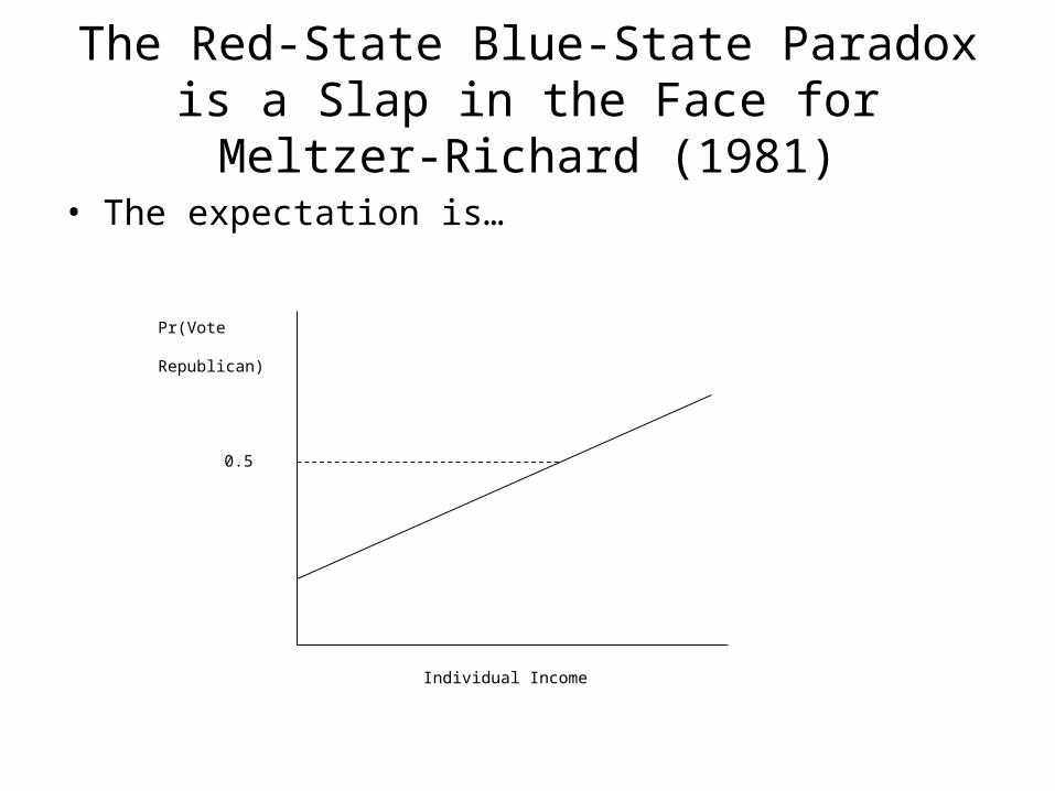
Andrew Gelman’s 2008 Decomposition of the Red-State Blue-State Paradox

Alternative Maps and Alternative Explanations

Created by G. Web, November 3rd, 2004 and posted on yakyak.org

Possible Explanations for the Puzzle

• Culture: Cultural conflicts (Hunter, 1992) the influence of religion (Himmelfarb, 1999) and self-sorting (Bishop, 2008).

• Economic Factors: Ansolabehere, Rodden, Snyder (2006)“Economic issues, not moral issues, have a much greater impacts on

voters’ decisions”

• Question: What economic interest could be at the root of the geographic divergence in preferences displayed in Gelman’s diagram? “Ultimately, individuals’ beliefs about what is the right or fair economic policy

for the nation are hard to explain. They are only related weakly to one common indicator of self-interest – income – and they are nearly uncorrelated with cultural issues.”

• Issue: The objective economic substrate that we would expect to underlie preferences for economic policy is not apparent.

The Argument

• I link the appearance of the Red-State/Blue-State paradox to economic factors (including increasing trade liberalization) that lowered earnings for the less-skilled.

• The “new, new trade theory” of Marc Melitz (2003), augmented by Davis and Harrigan (2007) to explain the loss of “Good Jobs,” helps us model and understand likely earnings loss and how this can vary with productivity by state.

• We have observed an increasing divergence between the states in the total factor productivity of their manufacturing firms (TFP) and likely the earnings of their lower-skilled workers.

• Given these developments, what preferences over government spending and services should we expect for residents of states with less productive firms?

Government Spending: Redistribution or Insurance?

• Moene and Wallerstein (2001): Employed, low-skill workers value government spending for two reasons. (1) Government spending can be redistributed back to them and (2) it provides insurance if they are unemployed.

• If all of government spending goes to the unemployed, then the desired amount of government taxation and spending falls with the earnings of the low-skilled (ceteris paribus).

• Insurance is a “normal” good.• Partisan preferences follow those over government spending.

0)1)(('),(

EL

L cuw

w

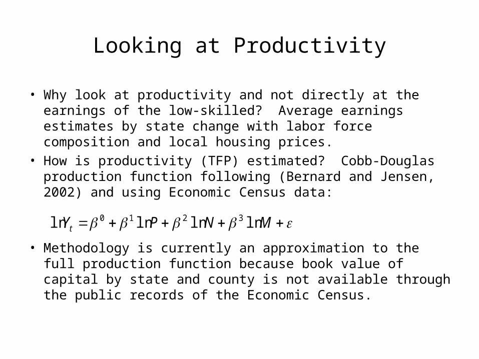
Looking at Productivity

• Why look at productivity and not directly at the earnings of the low-skilled? Average earnings estimates by state change with labor force composition and local housing prices.

• How is productivity (TFP) estimated? Cobb-Douglas production function following (Bernard and Jensen, 2002) and using Economic Census data:

• Methodology is currently an approximation to the full production function because book value of capital by state and county is not available through the public records of the Economic Census.

MNPYt lnlnlnln 3210

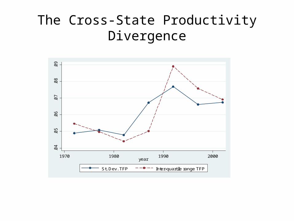
The Cross-State Productivity Divergence

.04

.05

.06

.07

.08

.09

1970 1980 1990 2000year

St. Dev. TFP Inter-quartile range TFP

The Cross-County Productivity Divergence

.12

.14

.16

.18

1970 1980 1990 2000year

St.Dev. TFP Inter-quartile range TFP

Modeling Votes

• Model of voting behavior estimated for the years 1992-2000 – the years after the emergence of inter-state differences in TFP and of the Red State – Blue State paradox.

• Specification:

% Voting Dem = f(Per capita Income, TFPJ, Demographics, Year Effects, State Fixed Effects, education, religion)

• Hypothesis: The coefficient on productivity should be positive.

Data and Measures for State/County Estimations

• Votes: David Leip’s Electoral Atlas website.

• Per capita income from BEA, Regional Economic Accounts. Deflated using a state-level COLI from Berry et al (2000).

• Data on racial composition from the Census Bureau’s Population Estimates Program.

• State-level Gini coefficient from the University of Texas Inequality Project.

• Percentage of adults 25+ with a BA interpolated from decennial census.

• Percentage of the population of a state that is counted as an adherent, ARDA decennial census of churches.

F.E. Models of State Vote Function 1992-2000

DV: Percent Democratic

(1) (2)PCSE

(3) (4)

Constant -32.3*** -95.9*** -40.9*** -36.5***

Real pci 0.73** 0.73*** 0.66* 0.65*

Productivity 15.53** 15.53*** 15.0** 13.69*

% Black 253.0*** 253.0*** 241.8*** 270.3***

% Hispanic 58.2** 58.2*** 60.9** 58.3**

Gini 64.7** 64.7*** 61.2* 65.9**

Election 1996 3.72*** 3.72*** 3.91*** 4.01***

Election 2000 -3.64*** -3.64*** -3.39*** -3.02*

% BA 62.9

% Adherents 11.4

R2 Within 0.74 0.74 0.75 0.75

Replication for Counties and IV estimation

DV = Democratic Percentage

(1)Counties

(2)State IV

Constant 33.1*** -33.4***

Real per cap income 0.84*** 0.67*

Productivity 1.48** 21.4**

% Black 69.4*** 272.9***

% Hispanic 1.74*** 71.2**

Gini 64.7**

Election 1996 -0.34*** 3.63***

Election 2000 -9.93*** -3.86***

R2 Within 0.70 0.74

F.E. Model for Individual-Level Effects

DV = Responses to Question on Gov’t Spending & Services (lower is more liberal)

(1)

Constant -0.92

State per cap Income 0.03

State Productivity -1.31*

State Prodv’ty*Higher Inc 1.11

Higher Income -0.05

Year 1994 0.21***

Year 1996 0.10*

N 3,094

R2 Within 0.02

Conclusion

• The explanation advanced here opens new lines of research focusing on the economic origins of the Red/Blue paradox.

• The theory advanced here relies on the growing divergence among American states in productivity of their firms and the earnings of their workers. Voters in states with declining productivity are turning away from government solutions, and this is strongest for lower-income voters.

• The theory does not help to explain the pattern Gelman observes among wealthy voters but does help to explain voter choices among the low-skilled.

• The theory also helps to explain a surge in “populist” Republican support.