BEGe pulse shape simulation - Max Planck Society · BEGe pulse shape simulation ... with a common trajectory ... Validation of the simulation Circular Scanning

BEGe pulse shape simulation

Matteo Agostini, Alberto Garfagnini, Calin A. Ur,

Enrico Bellotti, Assunta Di Vacri, Luciano Pandola

September 30th, 2009

Universita di Padova

1 / 11BEGe pulse shape simulation

N

Outline

Outline

1 The simulationI. The dynamics of electrons and photonsII. Signals induced by the charge motion inside the detectorIII. The total charge pulse and the preamplifier response

2 Validation of the simulation

3 MSE and SSE simulated signals

4 Summary


N

The simulation

The simulation structure

I. The dynamics of electrons and photons (MaGe)

<– the production processes of charged particles and photons–> the position and the type of the interaction with the germanium crystal–> the energy loss in each interaction

II. Signals induced by the charge motion inside the detector (MGS)

<– interaction coordinates–> trajectories–> signal induced on the electrodes

III. The total charge pulse and the preamplifier response

<– the energy loss in each interaction<– the signals induced by each interaction<– the preamplifier transfer function (PTF)–> the total charge pulse convolved with the PTF


N

The simulation

II. Signals induced by the charge motion inside thedetector - Trajectories

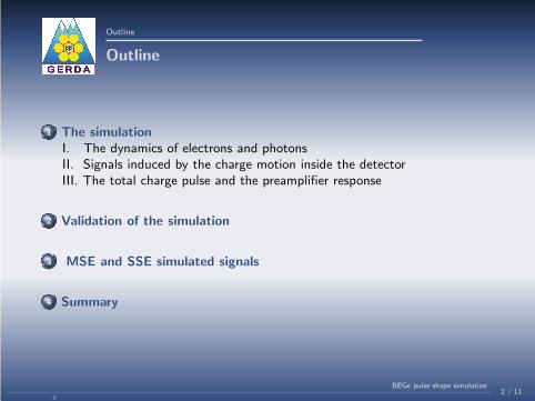
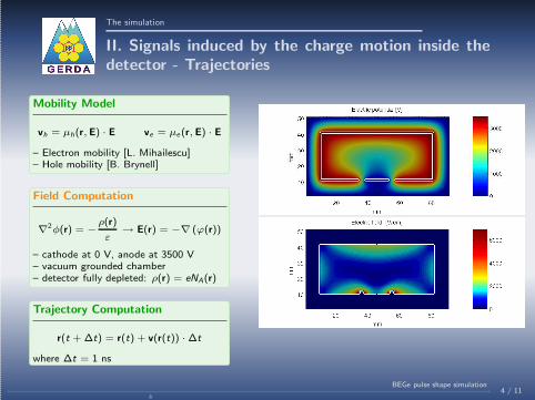
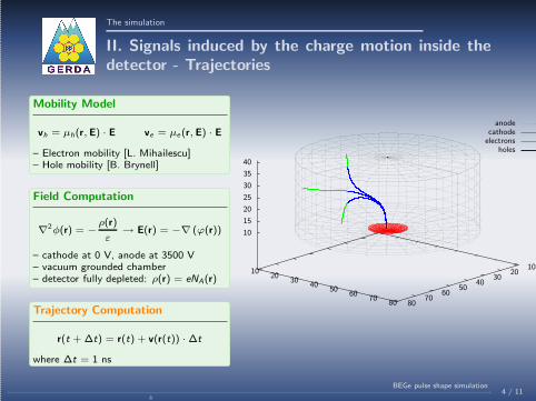
Mobility Model

vh = µh(r, E) · E ve = µe (r, E) · E

– Electron mobility [L. Mihailescu]– Hole mobility [B. Brynell]

Field Computation

∇2φ(r) = −

ρ(r)

ε→ E(r) = −∇ (ϕ(r))

– cathode at 0 V, anode at 3500 V– vacuum grounded chamber– detector fully depleted: ρ(r) = eNA(r)

Trajectory Computation

r(t + ∆t) = r(t) + v(r(t)) · ∆t

where ∆t = 1 ns


N

The simulation


Mobility Model

vh = µh(r, E) · E ve = µe (r, E) · E


Field Computation

∇2φ(r) = −

ρ(r)

ε→ E(r) = −∇ (ϕ(r))



r(t + ∆t) = r(t) + v(r(t)) · ∆t

where ∆t = 1 ns


N

The simulation


Mobility Model

vh = µh(r, E) · E ve = µe (r, E) · E


Field Computation

∇2φ(r) = −

ρ(r)

ε→ E(r) = −∇ (ϕ(r))



r(t + ∆t) = r(t) + v(r(t)) · ∆t

where ∆t = 1 ns

holeselectronscathode

anode

40

35

30

25

20

15

10

8070

6050

4030

2010

8070

6050

4030

2010


N

The simulation

II. Signals induced by the charge motion inside thedetector - Signal induced on the electrodes

Signal induced on a electrode

Shockley-Ramo Theorem :

Q(t) = −qφw (r(t))

where φw (r(t)) is the weighting potential.

The weighting potential is defined as the electric potential calculated when the considered

electrode is kept at a unit potential, all other electrodes are grounded and all charges inside the

device are removed.


N

The simulation

III. The total charge pulse and the preamplifierresponse

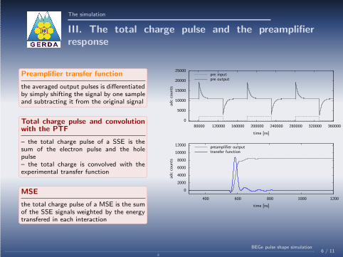
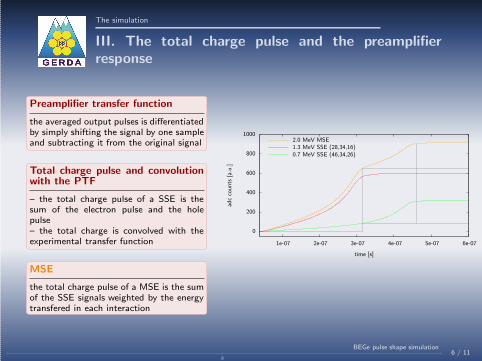
Preamplifier transfer function

the averaged output pulses is differentiatedby simply shifting the signal by one sampleand subtracting it from the original signal

Total charge pulse and convolutionwith the PTF

– the total charge pulse of a SSE is thesum of the electron pulse and the holepulse– the total charge is convolved with theexperimental transfer function

MSE

the total charge pulse of a MSE is the sumof the SSE signals weighted by the energytransfered in each interaction

pre outputpre input

time [ns]

adc

counts

36000032000028000024000020000016000012000080000

25000

20000

15000

10000

5000

0

transfer functionpreamplifier output

time [ns]

adc

counts

12001000800600400

12000

10000

8000

6000

4000

2000

0


N

The simulation






MSE


e pulseh pulsemgsmgs + pre

time [s]

adc

counts

4.5e-074e-073.5e-073e-072.5e-072e-071.5e-071e-075e-080

0.06

0.05

0.04

0.03

0.02

0.01

0

-0.01


N

The simulation






MSE


0

200

400

600

800

1000

1e-07 2e-07 3e-07 4e-07 5e-07 6e-07

adc

counts

[a.u

.]

time [s]

0.7 MeV SSE (46,34,26)1.3 MeV SSE (28,34,16)2.0 MeV MSE


N

Validation of the simulation

The validation measurements and the Averagingalgorithm

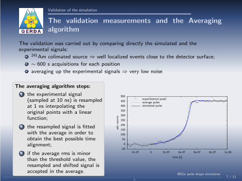
The validation was carried out by comparing directly the simulated and theexperimental signals:

241Am colimated source ⇒ well localized events close to the detector surface;

∼ 600 s acquisitions for each position

averaging up the experimental signals ⇒ very low noise

The averaging algorithm steps:

1 the experimental signal(sampled at 10 ns) is resampledat 1 ns interpolating theoriginal points with a linearfunction;

2 the resampled signal is fittedwith the average in order toobtain the best possible timealignment;

3 if the average rms is minorthan the threshold value, theresampled and shifted signal isaccepted in the average.

experimental pulseaverage pulsesimulated pulse

time [s]

adc

counts

1e-068e-076e-074e-072e-070-2e-07

500

450

400

350

300

250

200

150

100

50

0

-50


N


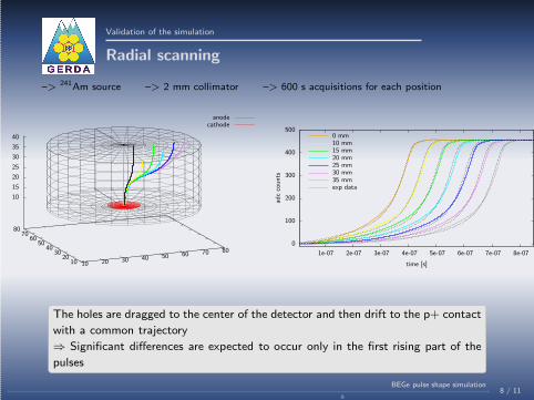
Radial scanning

–> 241Am source –> 2 mm collimator –> 600 s acquisitions for each position

cathodeanode

40

35

30

25

20

15

10

8070

6050

4030

2010

8070605040302010

exp data35 mm30 mm25 mm20 mm15 mm10 mm0 mm

time [s]

adc

counts

8e-077e-076e-075e-074e-073e-072e-071e-07

500

400

300

200

100

0

The holes are dragged to the center of the detector and then drift to the p+ contact

with a common trajectory

⇒ Significant differences are expected to occur only in the first rising part of the

pulses


N


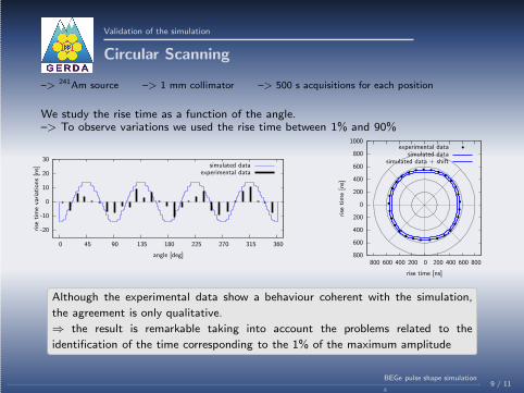
Circular Scanning

–> 241Am source –> 1 mm collimator –> 500 s acquisitions for each position

We study the rise time as a function of the angle.–> To observe variations we used the rise time between 1% and 90%

experimental datasimulated data

angle [deg]

rise

tim

eva

riat

ions

[ns]

36031527022518013590450

30

20

10

0

-10

-20

experimental datasimulated data

simulated data + shift

rise time [ns]

rise

tim

e[n

s]

8006004002000200400600800

1000

800

600

400

200

0

200

400

600

800

Although the experimental data show a behaviour coherent with the simulation,

the agreement is only qualitative.

⇒ the result is remarkable taking into account the problems related to the

identification of the time corresponding to the 1% of the maximum amplitude


N

MSE and SSE simulated signals

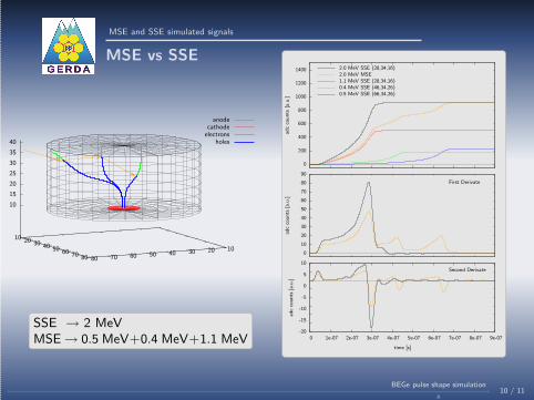
MSE vs SSE

holeselectronscathode

anode

40

35

30

25

20

15

10

8070605040302010

80 70 60 50 40 30 20 10

SSE → 2 MeVMSE → 0.5 MeV+0.4 MeV+1.1 MeV

-20

-15

-10

-5

0

5

10

0 1e-07 2e-07 3e-07 4e-07 5e-07 6e-07 7e-07 8e-07 9e-07

adc

counts

[a.u

.]

time [s]

Second Derivate

0

10

20

30

40

50

60

70

80

90

adc

counts

[a.u

.]

First Derivate

0

200

400

600

800

1000

1200

1400

adc

counts

[a.u

.]

0.5 MeV SSE (66,34,26)0.4 MeV SSE (46,34,26)1.1 MeV SSE (28,34,16)2.0 MeV MSE2.0 MeV SSE (28,34,16)


N

Summary

Summary

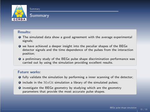
Results:

The simulated data show a good agreement with the average experimentalsignals;

we have achieved a deeper insight into the peculiar shapes of the BEGedetector signals and the time dependence of the pulses from the interactionposition;

a preliminary study of the BEGe pulse shape discrimination performance wascarried out by using the simulation providing excellent results.

Future works:

fully validate the simulation by performing a inner scanning of the detector;

include in the MaGe simulation a library of the simulated pulses;

investigate the BEGe geometry by studying which are the geometryparameters that provide the most accurate pulse shapes.


N

backup slides


N

Summary

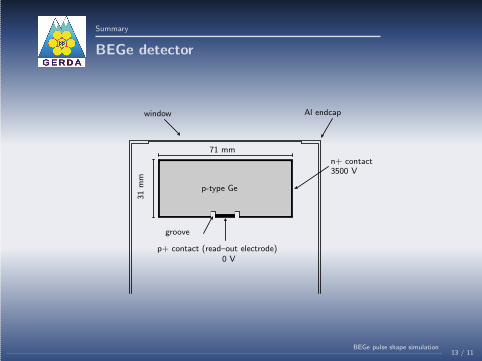
BEGe detector

71 mm

p+ contact (read–out electrode)

n+ contact

p-type Ge

3500 V

0 V

groove

31

mm

Al endcapwindow


Summary

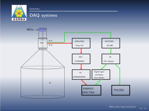
DAQ systems

PRE

BEGe

N2

AMPLIFIER

Ortec 672

ETHERNIM

DIGITIZER

N1728B

PC

GAMMAVISION

PC

TUC software

processing

PULSES

Digital signal

(Gast MWD)

SPECTRA

ENERGY

93 Ω

50 Ω

ADC


Summary

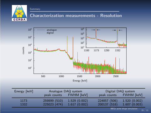
Characterization measurements - Resolution

1332125011731100

105

104

103

102

101

digitalanalogue

Energy [keV]

counts

2500200015001000500

106

105

104

103

102

101

Energy [keV] Analogue DAQ system Digital DAQ systempeak counts FWHM [keV] peak counts FWHM [keV]

1173 259899 (510) 1.529 (0.002) 224857 (506) 1.520 (0.002)1332 225023 (474) 1.617 (0.002) 200137 (518) 1.607 (0.003)


Summary

Characterization measurements - Linearity

digital electronicsanalogue electronics

Energy [keV]

chan

nel

300025002000150010005000

10000900080007000600050004000300020001000

0

digital electronicsanalogue electronics

Energy [keV]

300025002000150010005000

Energy [keV]

Ener

gy

[keV

]

25002000150010005000

1

0.5

0

-0.5

-1


Summary

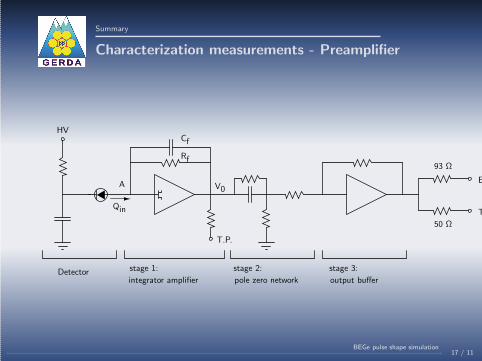
Characterization measurements - Preamplifier

HV

Detector

Qin

A

Cf

Rf

V0

stage 1:

integrator amplifier

stage 2:

pole zero network

stage 3:

output buffer

T.P.

93 Ω

50 Ω

Energy

Timinig


Summary

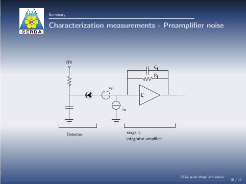
Characterization measurements - Preamplifier noise

HV

Detector

Cf

Rf

stage 1:

integrator amplifier

in

νn


Summary

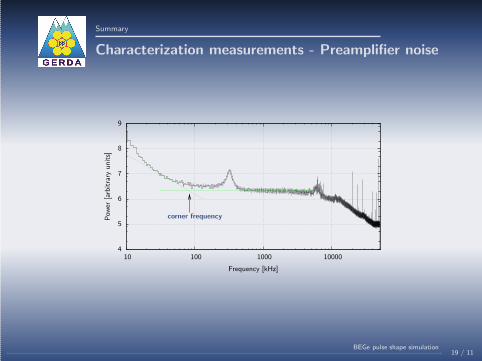
Characterization measurements - Preamplifier noise

corner frequency

Frequency [kHz]

Pow

er[a

rbitra

ryunits]

10000100010010

9

8

7

6

5

4


Summary

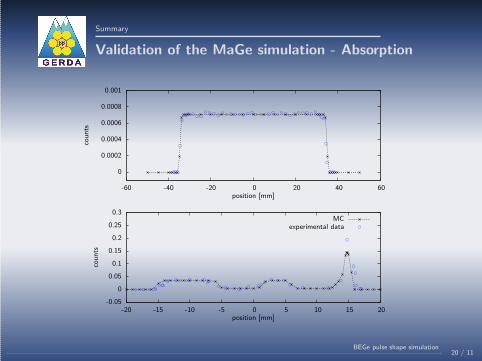
Validation of the MaGe simulation - Absorption

position [mm]

counts

6040200-20-40-60

0.001

0.0008

0.0006

0.0004

0.0002

0

experimental dataMC

position [mm]

counts

20151050-5-10-15-20

0.3

0.25

0.2

0.15

0.1

0.05

0

-0.05


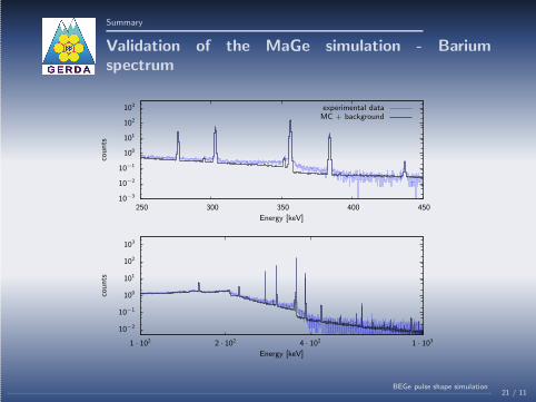
Summary

Validation of the MaGe simulation - Bariumspectrum

MC + backgroundexperimental data

Energy [keV]

counts

450400350300250

103

102

101

100

10−1

10−2

10−3

Energy [keV]

counts

1 · 1034 · 1022 · 1021 · 102

103

102

101

100

10−1

10−2


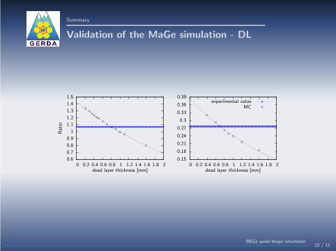
Summary

Validation of the MaGe simulation - DL

dead layer thickness [mm]

Rat

io

21.81.61.41.210.80.60.40.20

1.5

1.4

1.3

1.2

1.1

1

0.9

0.8

0.7

0.6

MCexperimental value

dead layer thickness [mm]21.81.61.41.210.80.60.40.20

0.39

0.36

0.33

0.3

0.27

0.24

0.21

0.18

0.15


Documents

BEGe pulse shape simulation - Max Planck Society · BEGe pulse shape simulation ... with a common trajectory ... Validation of the simulation Circular Scanning