Behavior in Strategic Settings: Evidence from a MillionRock-Paper-Scissors Games∗

Dimitris Batzilis† Sonia Jaffe‡ Steven Levitt§ John A. List¶

Jeffrey Picel‖

April 10, 2019

Abstract

We make use of data from a Facebook application where hundreds of thousands ofpeople played a simultaneous move, zero-sum game – rock-paper-scissors – with vary-ing information to analyze whether play in strategic settings is consistent with extanttheories. We report three main insights. First, we observe that most people employstrategies consistent with Nash, at least some of the time. Second, however, playersstrategically use information on previous play of their opponents, a non-Nash equilib-rium behavior; they are more likely to do so when the expected payoffs for such actionsincrease. Third, experience matters: players with more experience use information ontheir opponents more effectively than less experienced players, and are more likely towin as a result. We also explore the degree to which the deviations from Nash predic-tions are consistent with various non-equilibrium models. We analyze both a level-kframework and an adapted quantal response model. The naive version of each thesestrategies – where players maximize the probability of winning without considering theprobability of losing – does better than the standard formulation. While, one set ofpeople use strategies that resemble quantal response, there is another group of peoplewho employ strategies that are close to k1; for naive strategies the latter group is muchlarger.

JEL classification: C72, D03Keywords: play in strategic settings, large-scale data set, Nash equilibrium, non-equilibrium strategies

∗We would like to thank Vince Crawford for his insights, Colin Camerer, William Diamond, Teck Ho, ScottKominers, Jonathan Libgober, Guillaume Pouliot, and especially Larry Samuelson for helpful comments, theRoshambull development team for sharing the data, and Dhiren Patki and Eric Andersen for their researchassistance. All errors are our own.†Department of Economics, American College of Greece - Deree, dbatzilis@acg.edu‡(Corresponding author) Office of the Chief Economist, Microsoft, spj@uchicago.edu;§Department of Economics, University of Chicago and NBER, slevitt@uchicago.edu¶Department of Economics, University of Chicago and NBER, jlist@uchicago.edu‖Department of Economics, Harvard University, jpicel@fas.harvard.edu

Over the last several decades game theory has profoundly altered the social science land-

scape. Across economics and its sister sciences, elements of Nash equilibrium are included

in nearly every analysis of behavior in strategic settings. For their part, economists have

developed deep theoretical insights into how people should behave in a variety of important

strategic environments – from optimal actions during wartime to more mundane tasks such

as how to choose a parking spot at the mall. These theoretical predictions of game theory

have been tested in lab experiments (e.g. see cites in Camerer, 2003; Kagel and Roth, 1995),

and to a lesser extent in the field (e.g., Chiappori et al., 2002; Frey and Meier, 2004; Karlan,

2005; Walker and Wooders, 2001, and cites therein).

In this paper, we take a fresh approach to studying strategic behavior outside the lab,

exploiting a unique dataset that allows us to observe play while the information shown to

the player changes. In particular, we use data from over one million matches of rock-paper-

scissors1 played on a historically popular Facebook application. Before each match (made up

of multiple throws), players are shown a wealth of data about their opponent’s past history:

the percent of past first throws in a match that were rock, paper, or scissors, the percent of

all throws that were rock, paper, or scissors, and all the throws from the opponents’ most

recent five games. These data thus allow us to investigate whether, and to what extent,

players’ strategies incorporate this information.

The informational variation makes the strategy space for the game potentially much larger

than a one-shot rock-paper-scissors game. However, we show that in Nash Equilibrium,

players must expect their opponents to mix equally across rock-paper-scissors – same as in

the one-shot game. Therefore, a player has no use for information on her opponent’s history

when her opponent is playing Nash.

To the extent that an opponent systematically deviates from Nash, however, knowledge

of that opponent’s past history can potentially be exploited.2,3 Yet it is not obvious how

one should utilize the information provided. Players can use the information to determine

whether an opponent’s past play is consistent with Nash, but without seeing what informa-

1Two players each play rock, paper, or scissors. Rock beats scissors; scissors beats paper; paper beatsrock. If they both play the same, it is a tie. The payoff matrix is in Figure 3.

2If the opponent is not playing Nash, then Nash is no longer a best response. In symmetric zero-sumgames like RPS, deviating from Nash is costless if the opponent is playing Nash (since all strategies have anexpected payoff of zero), but if a player thinks he knows what non-Nash strategy his opponent is using thenthere is a profitable deviation from Nash.

3 Work in evolutionary game theory on rock-paper-scissors has looked at how the population’s distributionof strategies evolve towards or around Nash equilibrium (e.g., Hoffman et al., 2015; Cason et al., 2013). Pastwork on fictitious play has showed that responding to the opponents’ historical frequency of strategies leadsto convergence to Nash equilibrium Brown (1951); Berger (2005, 2007). Young (1993) also studies howconventions evolve as players respond to information about how their opponents have behaved in the past,while Mookherjee and Sopher (1994) and Mookherjee and Sopher (1997) examine the effect of informationon opponents’ history on strategic choices.

1

tion an opponent was reacting to (they do not observe the past histories of the opponent’s

previous opponents), it is hard to guess what non-Nash strategy the opponent may be using.

Additionally, players are not shown information about their own past play, so if a player

wants to exploit an opponent’s expected reaction, he has to keep track of his own history of

play.

Because of the myriad of possible responses, we start with a reduced-form analysis of the

first throw in each match to describe how players respond to the provided information. We

find that players use information: for example, they are more likely to play rock when their

opponent has played more scissors (which rock beats) or less paper (which beats rock) on

previous first throws, though the latter effect is smaller. When we do the analysis at the

player level, 47% of players are reacting to information about their opponents’ history in a

way that is statistically significant.4 Players also have a weak negative correlation across

their own first throws.

This finding motivated us to adopt a structural approach to evaluate the performance of

two well-known alternatives to Nash equilibrium: level-k and quantal response. The level-k

model posits that players are of different types according to the depth of their reasoning about

the strategic behavior of their opponents (Stahl, 1993; Stahl and Wilson, 1994, 1995; Nagel,

1995). Players who are k0 do not respond to information available about their opponent.

This can either mean that they play randomly (e.g., Costa-Gomes and Crawford, 2006)

or that they play some focal or salient strategy (e.g., Crawford and Iriberri, 2007; Arad

and Rubinstein, 2012). Players who are k1 respond optimally to a k0 player, which in our

context means responding to the focal strategy of the opponent’s (possibly skewed) historical

distribution of throws; k2 players respond optimally to k1, etc.5

Level-k theory acknowledges the difficulty of calculating equilibria and of forming equi-

librium beliefs, especially in one shot games. It has been applied to a variety of laboratory

games (e.g., Costa-Gomes et al., 2001; Costa-Gomes and Crawford, 2006; Hedden and Zhang,

2002; Crawford and Iriberri, 2007; Ho et al., 1998) and some naturally-occurring environ-

ments (e.g., Bosch-Domenech et al., 2002; Ostling et al., 2011; Gillen, 2009; Goldfarb and

Xiao, 2011; Brown et al., 2012). This paper has substantially more data than most other

level-k studies, both in number of observations and in the richness of the information struc-

ture. As suggested by an anonymous referee and acknowledged in Ho et al. (1998), the

implication of the fictitious play learning rule is that players should employ a k1 strategy,

4When doing a test at the player level, we expect about 5% of players to be false positives, so we takethese numbers as evidence on behavior only when they are statistically significant for substantially morethan 5% of players.

5Since the focal k0 strategies can be skewed, our k1 and k2 strategies usually designate a unique throw,which would not be true if k0 were constrained to be a uniform distribution.

2

best responding to the historical frequency of their opponents’ plays on the assumption that

it predicts their future choices. When k1 play is defined as the best response to past historical

play, as in the current context, it is of course indistinguishable from fictitious play.

We adapt level-k theory to our repeated game context. Empirically, we use maximum

likelihood to estimate how often each player plays k0, k1, and k2, assuming that they are

restricted to those three strategies. We find that the majority of play is best described as k0

(about 74%). On average, k1 is used in 18.5% of throws. The average k2 estimate is 7.7%,

but for only 12% of players do we reject at the 95% level that they never play k2. Most

players use a mixture of strategies, mainly k0 and k1.6 We also find that 20% of players

deviate significantly from 13, 13, 13

when playing k0. We also consider a cognitive hierarchy

version of the model and a naive version where players maximize the probability of winning

without worrying about losing. The rates of play of the analogous strategies are similar to

the baseline level-k, but the naive level-k is a better fit for most players.

We also show that play is more likely to be consistent with k1 when the expected return

to k1 is higher. This effect is larger when the opponent has a longer history – that is, when

the skewness in history is less likely to be noise. The fact that players respond to the level

of the perceived expected (k1) payoff, not just whether it is the highest payoff, is related to

the idea of quantal response: that players’ probability of using a pure strategy is increasing

in the relative perceived expected payoff of that strategy.7 This can be thought of as a

more continuous version of a k1 strategy. Rather than always playing the strategy with the

highest expected payoff as under k1, the probability of playing a strategy increases with the

expected payoff. As the random error in this (non-equilibrium) quantal response approaches

zero (or the responsiveness of play to the expected payoff goes to infinity) this converges to

the k1 strategy. On average, we find that increasing the expected payoff to a throw by one

standard deviation increases the probability it is played by 7.3 percentage points (more than

one standard deviation). The coefficient is positive and statistically significant for 63% of

players.

If players were using the k1 strategy, we would also find that expected payoffs have a

positive effect on probability of play. Similarly, if players used quantal response, many of

their throws would be consistent with k1 and our maximum likelihood analysis would indicate

6As we discuss in Section 4, there are several reasons that may explain why we find lower estimates for k1and k2 play than in previous work. Many players may not remember their own history, which is necessary forplaying k2. Also, given that k0 is what players would most likely play if they were not shown the information(i.e. when they play RPS outside the application), it may be more salient than in other contexts.

7Because we think players differ in the extent to which they respond to information and consider expectedpayoffs, we do not impose the restriction from Quantal Response Equilibrium theory (McKelvey and Palfrey,1995) that the perceived expected payoffs are correct. Instead, we require that the expected payoffs arecalculated based on the history of play. See Section 5 for more detail.

3

some k1 play. The above evidence does not allow us to state which model is a better fit for

the data. To test whether k1 or quantal response better explains play, we compare the model

likelihoods. The quantal response model is significantly better than the k1 model for 18.3

percent of players, yet the k1 model is significantly better for 17.5 percent of players. We

interpret this result as suggesting that there are some players whose strategies are close to

k1, or fictitious play, and a distinct set of players whose strategies resemble quantal response.

We also compare naive level-k to a naive version of the quantal response model. Here level-k

does better. About 12% of players significantly favor the quantal response model and 26%

significantly favor the naive level-k. The heterogeneity in player behavior points to the value

of studies like this one that have sufficient data to do within player analyses. In sum, our

data paint the picture that there is a fair amount of equilibrium play, and when we observe

non-Nash play, extant models have some power to explain the data patterns.

The remainder of the paper is structured as follows. Section 1 describes the Facebook

application in which the game is played and presents summary statistics of the data. Section 2

describes the theoretical model underlying the game, and the concept and implications of

Nash equilibrium in this setting. Section 3 explores how players respond to the information

about their opponents’ histories. Section 4 explains how we adapt level-k theory to this

context and provides parameter estimates. Section 5 adapts a non-equilibrium version of the

quantal response model to our setting. Section 6 compares the level-k and quantal response

models. Section 7 concludes.

1 Data: RoshambullRock-Paper-Scissors, also known as Rochambeau and jan-ken-pon, is said to have origi-

nated in the Chinese Han dynasty, making its way to Europe in the 18th century. To this

day, it continues to be played actively around the world. There is even a world Rock-Paper-

Scissors championship sponsored by Yahoo.8

The source of our data is an early Facebook ‘app’ called Roshambull. (The name is

a combination of Rochambeau and the name of the firm sponsoring the app, Red Bull.)

Roshambull allowed users to play rock-paper-scissors against other Facebook users – either

by challenging a specific person to a game or by having the software pair them with an

opponent. It was a very popular app for its era with 340,213 users (≈ 1.7% of Facebook

8Rock-paper-scissors is usually played for low stakes, but sometimes the result carries with it more seriousramifications. During the World Series of Poker, an annual $500 per person rock-paper-scissors tournamentis held, with the winner taking home $25,000. Rock-paper-scissors was also once used to determine whichauction house would have the right to sell a $12 million Cezanne painting. Christie’s went to the 11-year-oldtwin daughters of an employee, who suggested “scissors” because “Everybody expects you to choose ‘rock’.”Sotheby’s said that they treated it as a game of chance and had no particular strategy for the game, butwent with “paper” (Vogel, 2005).

4

users in 2007) starting at least one match in the first three months of the game’s existence.

Users played best-two-out-of-three matches for prestige points known as ‘creds.’ They could

share their records on their Facebook page and there was a leader board with the top players’

records.

To make things more interesting for players, before each match the app showed them

a “scouting sheet” with information on the opponent’s history of play.9 In particular, the

app showed each player the opponent’s distribution of throws on previous first throws of a

match (and the number of matches) and on all previous throws (and the number of throws),

as well as a play-by-play breakdown of the opponent’s previous five matches. It also shows

the opponent’s win-loss records and the number of creds wagered. Figure 1 shows a sample

screenshot from the game.

Our dataset contains 2,636,417 matches, all the matches played between May 23rd, 2007

(when the program first became available to users) and August 14th, 2007. For each throw,

the dataset contains a player ID, match number, throw number, throw type, and the time

and date at which the throw was made.10 This allows us to create complete player histories

at each point in time. Most players play relatively few matches in our three month window:

the median number of matches is 5 and the mean is 15.11 Figure 2 shows the distribution of

the number of matches a player played.

Some of our inference depends upon having a large number of observations per player;

for those sections, our analysis is limited to the 7758 “experienced” players for whom we

observe at least 100 clean matches. They play an average of 192 matches; the median is 148

and the standard deviation is 139.12 Because these are the most experienced players, their

strategies may not be representative; one might expect more sophisticated strategies in this

group relative to the Roshambull population as a whole.

Table 1 summarizes the play and opponents’ histories shown in the first throw of each

match, for both the entire sample and the experienced players. For all of the empirical

analysis we focus on the first throw in each match. Modeling non-equilibrium behavior on

9Bart Johnston, one of the developers said, “We’ve added this intriguing statistical aspect to thegame. . . You’re constantly trying to out-strategize your opponent” (Facebook, 2010).

10Unfortunately we only have a player id for each player; there is no demographic information or informa-tion about their out-of-game connections to other players.

11Because of the possibility for players to collude to give one player a good record if the other does notmind having a bad one, we exclude matches from the small fraction of player-pairs for which one player wonan implausibly high share of the matches (100% of ≥ 10 games or 80% of ≥ 20 games). To accurately recreatethe information that opponents were shown when those players played against others, we still include those“collusion” matches when forming the players’ histories.

12Depending on the opponent’s history, the strategies we look at may not indicate a unique throw (e.g. ifrock and paper have the same expected payoffs); for some analyses we only use players who have 100 cleanmatches where the strategies being considered indicate a unique throw, so we use between 5405 and 7758players.

5

Figure 1: Screenshot of the Roshambull App.

6

05.

0e+

041.

0e+

051.

5e+

05N

umbe

r of P

laye

rs

1 50 100 150 >200Number of Matches Played

Figure 2: Number of matches played by Roshambull users.Note: The figure shows the number of clean matches played by the 334,661 players who had at least one

clean, completed match (see Footnote 11 for a description of the data cleaning). The data has a very long

right tail, so all the players with over 200 matches are grouped together in the right-most bar.

7

Table 1: Summary Statistics of First Throws

Variable Full Sample Restricted Sample

Mean (SD) Mean (SD)

Throw Rock (%) 33.99 (47.37) 32.60 (46.87)Throw Paper (%) 34.82 (47.64) 34.56 (47.56)Throw Scissors (%) 31.20 (46.33) 32.84 (46.96)Player’s Historical %Rock 34.27 (19.13) 32.89 (8.89)Player’s Historical %Paper 35.14 (18.80) 34.88 (8.97)Player’s Historical %Scissors 30.59 (17.64) 32.23 (8.57)Opp’s Historical %Rock 34.27 (19.13) 33.59 (13.71)Opp’s Historical %Paper 35.14 (18.80) 34.76 (13.46)Opp’s Historical %Scissors 30.59 (17.64) 31.65 (12.84)Opp’s Historical Skew 10.42 (18.08) 5.39 (12.43)Opp’s Historical %Rock (all throws) 35.45 (12.01) 34.81 (8.59)Opp’s Historical %Paper (all throws) 34.01 (11.74) 34.10 (8.35)Opp’s Historical %Scissors (all throws) 30.54 (11.07) 31.09 (7.98)Opp’s Historical Length (matches) 55.92 (122.05) 99.13 (162.16)

Total observations 5,012,128 1,472,319

Note: The Restricted Sample uses data only from 7758 players who play at least 100 matches. The first3 variables are dummies for when a throw is rock, paper, or scissors (multiplied by 100). The next 3 arethe percentages of a player’s past throws that were each type, using only the first throw in each match.Variables 7-9 are the same as 4-6, but describing the opponents history of play instead of the player’s. “Allthrows” are the corresponding percentages for all of the opponent’s past throws. Opp’s Historical Length isthe number of previous matches the opponent played. Skew measures the extent to which the opponent’s

history of first throws deviates from random, 1100

∑i=r,p,s

(%i− 100

3

)2.

8

subsequent throws is more complicated because in addition to their opponent’s history, a

player may also respond to the prior throws in the match.

2 ModelA standard game of rock-paper-scissors is a simple 3 × 3 zero-sum game. The payoffs

are shown in Figure 3. Its only Nash Equilibrium is for players to mix 13, 13, 13

across rock,

paper, and scissors. Because each match is won by the first player to win two throws, and

players play multiple matches, the strategies in Roshambull are potentially substantially

more complicated: players could condition their play on various aspects of their own or

their opponents’ histories. A strategy would be a mapping from (1) the match history for

the current match so far, (2) one’s own history of all matches played, and (3) the space

of information one might be shown about one’s opponent’s history, onto a distribution of

throws. In addition, Roshambull has a matching process operating in the background, in

which players from a large pool are matched into pairs to play a match and then are returned

to the pool to be matched again. In the Appendix, we formalize Roshambull in a repeated

game framework.

Player 2:Rock Paper Scissors

Player 1:Rock (0,0) (-1,1) (1,-1)Paper (1,-1) (0,0) (-1,1)

Scissors (-1,1) (1,-1) (0,0)

Figure 3: Payoffs for a single throw of rock-paper-scissors.

Despite the potential for complexity, we show the equilibrium strategies are still simple.

Proposition 1. In any Nash Equilibrium, for every throw of every match, each player

correctly expects his opponent to mix 13, 13, 13over rock, paper, and scissors.13

Proof. See the Appendix.

The proof shows that, since it is a symmetric, zero-sum game, players’ continuation values

at the end of every match must be zero. Therefore players are only concerned with winning

the match, and not with the effect of their play on their resulting history. We then show that

for each throw in the match, if player A correctly believes that player B is not randomizing13, 13, 13, then player A has a profitable deviation.

Same as in the single-shot game, Nash Equilibrium implies that players randomize 13, 13, 13

both unconditionally and conditional on any information available to their opponent. Out

13Players could use aspects of their history that are not observable to the opponent as a private random-ization devices, but conditional on all information available to the opponent, they must be mixing 1

3 ,13 ,

13 .

9

of equilibrium, players may condition their throws on their or their opponents’ histories in a

myriad of ways. The resulting play may or may not result in an unconditional distribution

of play that differs substantially from 13, 13, 13. In Section 3, we present evidence that 82%

of experienced players have first throw distributions that do not differ from 13, 13, 13, but

half respond to their opponents’ histories.14 While non-random play and responding to

information is consistent with Nash beliefs – if the opponent is randomizing 13, 13, 13

then any

strategy gives a zero expected payoff – it is not consistent with Nash Equilibrium because

the opponent would exploit that predictability.

3 Players respond to informationBefore examining the data for specific strategies players may be using, we present reduced-

form evidence that players respond to the information available to them. To keep the pre-

sentation clear and simple, for each analysis we focus on rock, but the results for paper and

scissors are analogous, as shown in the Appendix.

We start by examining the dispersion across players in how often they play rock. Figure 4

shows the distribution across experienced players of the fraction of their last 100 throws that

are rock.15 It also shows the binomial distribution of the fraction of 100 i.i.d. throws that

are rock if rock is always played 13

of the time. The distribution from the actual data is

substantially more dispersed than the theoretical distribution, suggesting that the fraction

of rock played deviates from one-third more than one would expect from pure randomness.

Doing a chi-squared test on all throws at the player level, we reject16 uniform random play

for 18% of experienced players. The rejection rate is lower for less experienced players, but

this seems to be due to power more than differences in play. Players who go on to play more

games are actually less likely to have their histories deviate significantly from Nash after 20

or 30 games than players who play fewer total games.

Given this dispersion in the frequency with which players play rock, we test whether

players respond to the information they have about their opponents tendency to play rock –

the opponents’ historical rock percentage. Table 2 groups throws into bins by the opponents’

historical percent rock and reports the fraction of paper, rock, and scissors played. Note that

the percent paper is increasing across the bins and percent scissors is decreasing. Paper goes

from less than a third chance to more than a third chance (and scissors goes from more to

less) right at the cutoff where rock goes from less often than random to more often than

14We also find serial correlation both across throws within a match and across matches, which is inconsis-tent with Nash Equilibrium.

15Inexperienced players also have a lot of variance in the fraction of time they play rock, but for them itis hard to differentiate between deviations from 1

3 ,13 ,

13 and noise from randomization.

16If all players were playing Nash, we would expect to reject the null for 5% of players; with 95% probabilitywe would reject the null for less than 5.44% of players.

10

020

040

060

080

0N

umbe

r of P

laye

rs

0 20 40 60 80 100Number of rock in last 100 throws

Actual Binomial7758 Players

Figure 4: Percent of last 100 Throws that are Rock – Observed and PredictedNote: For each of the 7758 players with at least 100 matches we calculate the percent of his or her last 100

throws that were rock (purple distribution). We overlay the binomial distribution with n = 100 and p = 13 .

Table 2: Response to Percent Rock

Opp’s Historical % Throws (%)

Paper Rock Scissors N

0% - 25% 27.07 35.84 37.09 1,006,72625% - 30% 27.11 35.23 37.66 728,408

30% - 3313

% 29.87 34.72 35.41 565,623

3313

% - 37% 34.21 34.44 31.35 794,88637% - 42% 40.45 32.58 26.97 529,71042% - 100% 46.58 30.35 23.06 1,056,162

Note: Matches are binned by the opponent’s historical percent of rock on first throws prior to the match.

For each range of opponents’ historical percent rock, this table reports the distribution of rock, paper, and

scissors throws the players use.

11

random.17 The percent rock a player throws does not vary nearly as much across the bins.

For a more thorough analysis of how this and other information presented to players

affects their play, Table 3 presents regression results. The dependent variable is binary, in-

dicating whether a player throws rock. The coefficients all come from one linear probability

regression. The first column is the effect for all players, the second column is the additional

effect of the covariates for players in the restricted sample; the third column is the addi-

tional effect for those players after their first 99 games. For example, a standard deviation

increase in the opponent’s historical fraction of scissors (.176) increases the probability that

an inexperienced player plays rock by 4.2 percentage points (100 × .176 × .2376); for an

experienced player who already played at least 100 games, the increase is 9.4 percentage

points (100× .176× (.2376 + .1556 + .1381)).

As expected, the effects of the opponent’s percent of first throws that were paper is

negative and the effect for scissors is positive and both get stronger with experience.18 This

finding adds to the evidence that experience leads to the adoption of more sophisticated

strategies Nagel (1995); Weber (2003). The effect of the opponent’s distribution of all throws

and the opponent’s lagged throws is less clear.19 The consistent and strong reactions to the

opponent’s distribution of first throws motivates our use of that variable in the structural

models. If we do the analysis at the player level, the coefficients on opponents’ historical

distributions are statistically significant for 47% of experienced players.

The fact that players respond to their opponents’ histories makes their play somewhat

predictable and potentially exploitable. To look at whether opponents exploit this pre-

dictability, we first run the regression from Table 3 on half the data and use the coefficients

to predict for the other half – based on the opponent’s history – the probability of playing

rock on each throw. We do the same for paper and scissors. Given the predicted probabilities

of play, we calculate the expected payoff to an opponent of playing rock. Table 4 bins throws

by the opponents’ expected payoff to playing rock and reports the distribution of opponent

throws. The probability of playing rock bounces around – if anything, opponents are less

likely to play rock when the actual expected payoff is high – the opposite of what we would

expect if the predictability of players’ throws were effectively exploited.

Another way of measuring of the ability to exploit predictability is looking at the win and

17If players were truly, strictly maximizing their payoff against the opponent’s past distribution, thischange would be even more stark, though it would not go exactly from 0 to 1 since the optimal responsealso depends on the percent of paper (or scissors) played, which the table does not condition on.

18The Appendix has the same table adding own history. The coefficients on opponent’s history are basicallyunaffected. The coefficients on own history reflect the imperfect randomization – players who played rock inthe past are more likely to play rock.

19If we run the regression with just the distribution of all throws or just the lags, the signs are as expected,but that seems to be mostly picking up the effect via the opponent’s distribution of first throws.

12

Table 3: Probability of Playing Rock

Covariate Dependent Var: Dummy for Throwing Rock

(1) (2) (3)Opp’s Fraction Paper (first) -0.0382*** -0.0729*** -0.0955***

(0.0021) (0.0056) (0.0087)Opp’s Fraction Scissors (first) 0.2376*** 0.1556*** 0.1381***

(0.0022) (0.0060) (0.0094)Opp’s Fraction Paper (all) 0.0011 0.0258** 0.0033

(0.0032) (0.0088) (0.0138)Opp’s Fraction Scissors (all) 0.0416*** 0.0231* -0.0208

(0.0033) (0.0093) (0.0146)Opp’s Paper Lag 0.0052*** -0.0019 -0.0043*

(0.0007) (0.0015) (0.0019)Opp’s Scissors Lag 0.0139*** 0.0055*** -0.0017

(0.0008) (0.0016) (0.0020)Own Paper Lag -0.0171*** 0.0239*** 0.0051**

(0.0007) (0.0015) (0.0019)Own Scissors Lag -0.0145*** 0.0208*** -0.0047*

(0.0007) (0.0015) (0.0019)Constant 0.3548*** -0.0264*** -0.0009

(0.0006) (0.0014) (0.0018)R2 0.0172N 4,433,260

Note: The table shows OLS coefficients from a single regression of a throw being rock on the covariates.

The first column is the effect for all players; the second column is the additional effect of the covariates for

players in the restricted sample; the third column is the additional effect for those players after their first 100

games. Opp’s Fraction Paper (Opp’s Fraction Paper (all)) refers to the fraction of the opponent’s previous

first throws (all throws) that were paper. Opp’s Paper Lag (Own Paper Lag) is a dummy for whether the

opponent’s (player’s own) most recent first throw in a match was paper. The Scissor variables are defined

analogously for scissors. The regressions also control for the opponent’s number of previous matches.

13

Table 4: Opponents’ Response to Expected Payoff of Rock

Opponent’s Expected Opponent’s Throw (%) N

Payoff of Rock Paper Rock Scissors

[−1, −0.666] 30.83 40.56 28.61 2,754

[−0.666, −0.333] 32.89 38.56 28.55 65,874

[−0.333, 0] 33.83 34 32.17 1,266,538

[0, 0.333] 35.52 32.45 32.03 871,003

[0.333, 0.666] 34.4 34.47 31.13 12,234

Note: The expected payoff to rock is calculated by running the specification from Table 3 for paper and

scissors on half the data, using the coefficients to predict the probability of playing paper minus the proba-

bility of playing scissors for each throw in the other half of the sample. This table shows the distribution of

opponents’ play for different ranges of that expected payoff.

Table 5: Win Percentages

Wins (%) Draws (%) Losses (%)Wins (%)− Losses (%)

N

Full Sample 33.8 32.4 33.8 0 5,012,128

Experienced Sample 34.66 32.17 33.17 1.49 1,472,319

Best Response toPredicted Play

41.66 30.97 27.37 14.29 2,218,403

Note: Experienced Sample refers to players who play at least 100 games. “Best Response” is how a player

would do if she always played the best response to players’ predicted play: the specification from Table 3

(and analogous for paper and scissors) is run on half the data and the coefficients used to predict play for

the other half. Wins-Losses shows the expected winnings per throw if players bet $100 on a throw.

14

loss rates. We calculate how often an opponent who responded optimally to the predicted

play would win, draw, and lose. We compare these to the rates for the full sample and the

experienced sub-sample, keeping in mind that responding to this predicted play optimally

would require that the opponent know his own history. Table 5 presents the results. An

opponent best responding would win almost 42% of the time. If players bet $1 on each throw,

the expected winnings is equal to the probability that they win minus the probability that

they lose. The average experienced player would win 1.49¢ on the average throw (34.66%

- loss 22.17%=1.49), but someone responding optimally to the predictability would win

14.3¢ on average (41.66% - 27.37%=14.29). (A player playing Nash always breaks even on

average.) Though experienced players do better (as previous work has shown (e.g., Nagel,

1995; Weber, 2003)), these numbers indicate that even experienced players are not fully

exploiting others’ predictability.

Since players are responding to their opponent’s history, exploiting those responses re-

quires that a player remember her own history of play (since the game does not show one’s

own history). So it is perhaps not surprising that players’ predictability is not exploited and

therefore unsurprising that they react in a predictable manner. Having described in broad

terms how players react to the information presented, we turn to existing structural models

to test whether play is consistent with these hypothesized non-equilibrium strategies.

4 Level-k behaviorWhile level-k theory was developed to analyze single shot games, it is a useful framework

for exploring how players use information about their opponent. The k0 strategy is to ignore

the information about one’s opponent and play a (possibly random) strategy independent

of the opponent’s history. While much of the existing literature assumes that k0 is uniform

random, some studies assume that k0 players use a salient or focal strategy. In this spirit,

we allow players to randomize non-uniformly (imperfectly) when playing k0 and assume that

the k1 strategy best responds to a focal strategy for the opponent – k1 players best respond

to the opponent’s past distribution of first throws.20 It seems natural that a k1 player who

assumes his opponent is non-strategic would use this description of past play as a predictor

of future play.21 When playing k2, players assume that their opponents are playing k1 and

respond accordingly.

Formal definitions of the different level-k strategies in our context are as follows:

Definition. When a player uses a k0 strategy in a match, his choice of throw is unaffected

20The reduced form results indicate that players react much more strongly to the distribution of firstthrows than to the other information provided.

21Alternatively, a k1 player may think that k0 is strategic, but playing an unknown strategy so past playis the best predictor of future play.

15

by his history or his opponent’s history.

We should note that using k0 is not necessarily unsophisticated. It could be playing

the Nash equilibrium strategy. However there are two reasons to think that k0 might not

represent sophisticated play. First, for some players the frequency distribution of their k0

play differs significantly from 13, 13, 13, suggesting that if they are trying to play Nash, they are

not succeeding. Second, more subtly, it is not sophisticated to play the Nash equilibrium if

your opponents are failing to play Nash. With most populations who play the beauty contest

game, people who play Nash do not win (Nagel, 1995). In RPS, if there is a possibility that

one’s opponent is playing something other than Nash, there is a strategy that has a positive

expected return, whereas Nash always has a zero expected return. (If it turns out the

opponent is playing Nash, then every strategy has a zero expected return and so there is

little cost to trying something else.) Given that some players differ from 13, 13, 13

when playing

k0 and most don’t always play k0, Nash is frequently not a best response.22

Definition. When a player uses the k1 strategy in a match, he plays the throw that has

the highest expected payoff if his opponent randomizes according to that opponent’s own

historical distribution of first throws.

We have not specified how a player using k0 chooses a throw, but provided the process

is not changing over time, his past throw history is a good predictor of play in the current

match. To calculate the k1 strategy for each throw, we calculate the expected payoff to each

of rock, paper, and scissors against a player who randomizes according to the distribution of

the opponent’s history. The k1 strategy is the throw that has the highest expected payoff. (As

discussed earlier, it is by definition the same as the strategy that would have been chosen

by under fictitious play.) Note that this is not always the one that beats the opponent’s

most frequently played historical throw, because it also accounts for the probability of losing

(which is worse than a draw).23

Definition. When a player uses the k2 strategy in a match, he plays the throw that is the

best response if his opponent randomizes uniformly between the throws that maximize the

opponent’s expected payoff against the player’s own historical distribution.

The k2 strategy is to play “the best response to the best response” to one’s own history.

In this particular game k2 is in some sense harder than k1 because the software shows only

one’s opponent’s history, but players could keep track of their own history.

22Nash always has an expected payoff of zero. As show in Table 5, best responding can have an expectedpayoff of 14¢ for every dollar bet.

23 Sometimes opponents’ distributions are such that there are multiple throws that are tied for the highestexpected payoff. For our baseline specification we ignore these throws. As a robustness check we definealternative k1−strategies where one throw is randomly chosen to be the k1 throw when payoffs are tiedor where both throws are considered consistent with k1 when payoffs are tied. The results do not changesubstantially.

16

Both k1 and k2 depend on the expected payoff to each throw given the assumed beliefs

about opponents’ play. We calculate the expected payoff by subtracting the probability of

losing the throw from the probability of winning the throw, thereby implicitly assuming that

players are myopic and ignore the effect of their throw on their continuation value.24 This

approach is consistent with the literature that analyzes some games as “iterated play of a

one-shot game” instead of as an infinitely repeated game (Monderer and Shapley, 1996).

More generally, we think it is a reasonable simplifying assumption. While it is possible

one could manipulate one’s history to affect future payoffs with an effect large enough to

outweigh the effect on this period’s payoff, it is hard to imagine how.25

Having defined the level-k strategies in our context, we now turn to the data for evidence

of level-k play.

4.1 Reduced-form evidence for level-k play

One proxy for k1 and k2 play is players choosing throws that are consistent with these

strategies. Whenever a player plays k1 (or k2) her throw is consistent with that strategy.

However, the converse is not true. Players playing the NE strategy of 13, 13, 13

would, on

average, be consistent with k1 a third of the time.

For each player we calculate the fraction of throws that are k1-consistent; these fractions

are upper bounds on the amount of k1 play. No player with more than 20 matches always

plays consistent with k1. The highest percentage of k1-consistent behavior for an individual

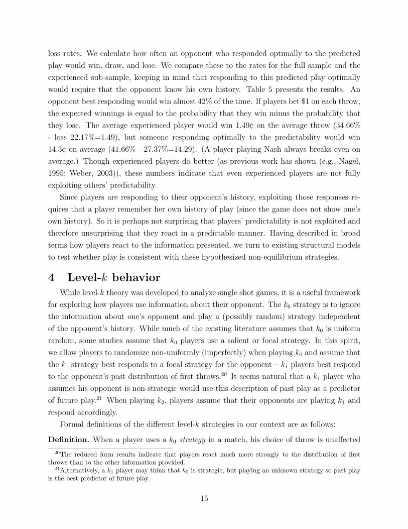
in our experienced sample is 84 percent. Figure 5a shows the distribution of the fraction

of k1-consistency across players. It suggests that at least some players use k1 at least some

of the time: the distribution is to the right of the vertical 13-line and there is a substantial

right tail. To complement the graphical evidence, we formally test whether the observed

frequency of k1-consistent play is significantly greater than expected under random play.

For each player with at least 100 games, we calculate the probability of observing at least as

many throws consistent with k1 if the probability of a given throw being k1-consistent were

only 1/3. The probability is less than 5% for 47% of players.

Given that players seem to play k1 some of the time, players could benefit from playing k2.

Figure 5b shows the distribution of the fraction of actual throws that are k2-consistent. The

24In the proof of Proposition 1 we show that in Nash Equilibrium, histories do not affect continuationvalues, so in equilibrium it is a result, not an assumption, that players are myopic. However, out of NashEquilibrium, it is possible that what players throw now can affect their probability of winning later rounds.

25One statistic that we thought might affect continuation values is the skew of a player’s historical dis-tribution. As a player’s history departs further from random play, there is more opportunity for opponentresponse and player exploitation of opponent response. We ran multinomial logits for each experienced playeron the effect of own history skewness on the probability of winning, losing or drawing. The coefficients weresignificant for less than (the expected false positives of) 5% of players. This provides some support to ourassumption that continuation values are not a primary concern.

17

(a) (b)

Figure 5: Level-k consistencyNote: These graphs show the distribution across the 6674 players who have 100 games with uniquely defined

k1 and k2 strategies of the fraction of throws that are k1- and k2-consistent. The vertical line indicates 13 ,

which we would expect to be the mean of the distribution if throws were random.

observed frequency of k2 play is slightly to the left of that expected with random play, but

we cannot reject random play for a significant number of players. This lack of evidence for

k2 play is perhaps unsurprising given that players are not shown the necessary information.

If we assume that players use either k0, k1, or k2 then we can get a lower bound on the

amount of k0. For each player we calculate the percentage of throws that are consistent

with neither k1 nor k2. We do not expect this bound to be tight because, in expectation, a

randomly chosen k0 play will be consistent with either the k1 or k2 strategy about 13

+ (1−13)× 1

3≈ .56 of the time. The mean lower bound across players with at least 100 matches is

37 percent. The minimum is 8.2 percent and the maximum is 77 percent.

The players do have an incentive to use these strategies. Averaging across the whole

dataset, always playing k1 would allow a player to win 35.09% (and lose 32.61%) of the

time. If a player always played k2 he would win 42.68% (and lose 27.74%) of the time.

While these numbers may be surprising, if an opponent plays k1 just 14% of the time and

plays randomly the rest of the time, the expected win rate from always play k2 would be

.14×1+ .86× .33 = .426. It seems that memory or informational constraints prevent players

from employing what would be a very effective strategy.

4.1.1 Multinomial Logit

Before turning to the structural model, we can use a multinomial logit model to explore

whether a throw being k1-consistent increases the probability that a player chooses that

throw. For each player, we estimate a multinomial logit where the utilities are

U ji = αj + β · 1{k1,i = j}+ εji ,

18

020

040

060

080

0N

umbe

r of P

laye

rs

-1 0 1 2 3Logit Coefficient

SignificantAll

6856 Players, 3 outliers omitted

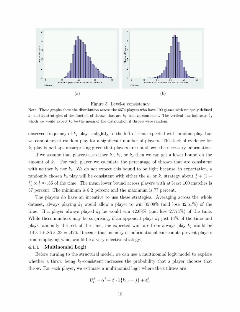
Figure 6: Coefficient in the k1 multinomial logit.Note: The coefficient is β from the logit estimation, run separately for each player, Urock

i = αrock +β ·krock1,i +

εrocki , analogously for paper and scissors, where krock1, is a dummy for whether rock is the k1-consistent thing

to do on throw i. Outliers more than 4 standard deviations from the mean are omitted.

where j = r, p, s and 1{k1,i = i} is an indicator for when j is the k1-consistent action for

throw i. Figure 6 shows the distribution of β’s across players. The mean is .52.

The marginal effect varies slightly with the baseline probabilities, ∂Pr{i}∂xi

= β×Pr{i}(1−Pr{i}), but is approximately 1

3

(1− 1

3

)= 2

9times the coefficient. Hence, on average, a throw

being k1-consistent means it is 12 percentage points more likely to be played. Given that the

standard deviation across experienced players in the percent of rock, paper, or scissors throws

is about 5 percentage points, this is a large average effect. The individual-level coefficient is

positive and significant for 64 percent of players.

4.2 Maximum likelihood estimation of a structural model of level-

k thinkingThe results presented in the previous sections provide some evidence as to what strategies

are being employed by the players in our sample, but they do not allow us to identify with

precision the frequency with which strategies are employed – we can say that throws are k1

more often than would happen by chance, but cannot estimate what fraction of the time

a player is playing a throw because it is k1. To obtain point estimates of each player’s

proportion of play by level-k, along with standard errors, we need additional assumptions.

Assumption 1. All players use only the k0, k1, or k2 strategies in choosing their actions.

19

Assumption 1 restricts the strategy space, ruling out any approach other than level-k,

and also restricting players not to use levels higher than k2. We limit our modeling to levels

k2 and below, both for mathematical simplicity and because there is little reason to believe

that higher levels of play are commonplace, both based on the low rates of k2 play in our

data, and rarity of k3 and higher play in past experiments.26

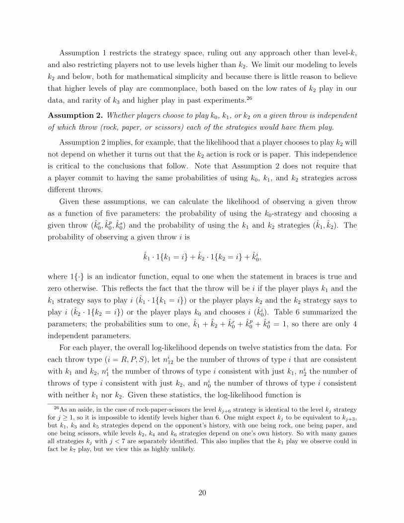
Assumption 2. Whether players choose to play k0, k1, or k2 on a given throw is independent

of which throw (rock, paper, or scissors) each of the strategies would have them play.

Assumption 2 implies, for example, that the likelihood that a player chooses to play k2 will

not depend on whether it turns out that the k2 action is rock or is paper. This independence

is critical to the conclusions that follow. Note that Assumption 2 does not require that

a player commit to having the same probabilities of using k0, k1, and k2 strategies across

different throws.

Given these assumptions, we can calculate the likelihood of observing a given throw

as a function of five parameters: the probability of using the k0-strategy and choosing a

given throw (kr0, kp0, k

s0) and the probability of using the k1 and k2 strategies (k1, k2). The

probability of observing a given throw i is

k1 · 1{k1 = i}+ k2 · 1{k2 = i}+ ki0,

where 1{·} is an indicator function, equal to one when the statement in braces is true and

zero otherwise. This reflects the fact that the throw will be i if the player plays k1 and the

k1 strategy says to play i (k1 · 1{k1 = i}) or the player plays k2 and the k2 strategy says to

play i (k2 · 1{k2 = i}) or the player plays k0 and chooses i (ki0). Table 6 summarized the

parameters; the probabilities sum to one, k1 + k2 + kr0 + kp0 + ks0 = 1, so there are only 4

independent parameters.

For each player, the overall log-likelihood depends on twelve statistics from the data. For

each throw type (i = R,P, S), let ni12 be the number of throws of type i that are consistent

with k1 and k2, ni1 the number of throws of type i consistent with just k1, n

i2 the number of

throws of type i consistent with just k2, and ni0 the number of throws of type i consistent

with neither k1 nor k2. Given these statistics, the log-likelihood function is

26As an aside, in the case of rock-paper-scissors the level kj+6 strategy is identical to the level kj strategyfor j ≥ 1, so it is impossible to identify levels higher than 6. One might expect kj to be equivalent to kj+3,but k1, k3 and k5 strategies depend on the opponent’s history, with one being rock, one being paper, andone being scissors, while levels k2, k4 and k6 strategies depend on one’s own history. So with many gamesall strategies kj with j < 7 are separately identified. This also implies that the k1 play we observe could infact be k7 play, but we view this as highly unlikely.

20

Table 6: Parameters of the Structural Model

Variable Definition

kr0 fraction of the time a player plays k0 and chooses rock

kp0 fraction of the time a player plays k0 and chooses paper

ks0 fraction of the time a player plays k0 and chooses scissors

k1 fraction of the time a player plays k1(k2) 1− k1 − kr0 − k

p0 − ks0 (not an independent parameter)

Note: kr0 is not equal to the fraction of k0 throws that are rock; that conditional probability is given bykr0

kr0+kp

0+ks0

.

L(k1, k2, kr0, k

p0, k

s0) =∑

i = r, p, s

(ni12 ln(k1 + k2 + ki0) + ni1 ln(k1 + ki0) + ni2 ln(k2 + ki0) + ni0 ln(ki0)

).

For each experienced player we use maximum likelihood to estimate(k1, k2, k

r0, k

p0, k

s0

).27

Given the estimates, standard errors are calculated analytically.28

This approach allows us to not count as k1 those throws that are likely k0 or k2 and

only coincidentally consistent with k1; it is more sophisticated than simply looking at the

difference between the rate of k1-consistency and 1/3 as we do in Figure 5a. If a player is

biased towards playing rock and rock is the k1 move in disproportionately many of their

matches, we would not want to count those plays as k1. Conversely, if a player always

played k1, we would not want to say that 1/3 of those were due to chance. Essentially, the

percentage of the time a player uses the k1 strategy is estimated from the extent to which

that player is more likely to play rock (or paper or scissors) when it is k1-consistent than

when it is not k1-consistent.

Table 7 summarizes the estimates of k0, k1, and k2: the average player uses k0 for 73.8

percent of throws, k1 for 18.5 percent of throws and k2 for 7.7 percent of throws. Weighting

by the precision of the estimates or by the number of games does not change these results

substantially. As the minimums and maximums suggest, these averages are not the result of

some people always playing k1 while others always play k2 or k0. Most players mix, using a

combination of mainly k0 and k1.29

Table 8 reports the share of players for whom we can reject with 95 percent confidence

27Since we do the analysis within player, the estimates would be very imprecise for players with fewergames.

28We derive the Hessian of the likelihood function, plug in the estimates, and take the inverse.29Other work, such as (Georganas et al., 2014), has found evidence of players mixing levels of sophistication

across different games.

21

Table 7: Summary of k0, k1, and k2 estimates.

Variable Mean SD Median Min Max

k0 0.738 0.16 0.75 0.19 1.00k1 0.185 0.14 0.16 0.00 0.77k2 0.077 0.08 0.06 0.00 0.41N = 6, 639

Note: Based on the 6639 players with 100 clean matches with well-defined k1 and k2 strategies.

Table 8: Percent of players we reject always or never playing a strategy.

Variable 95% CI does notinclude 0

95% CI does notinclude 1

95% CI does notinclude 0 or 1

k0 93.11% 58.30% 57.51%k1 62.87% 99.97% 62.87%k2 11.54% 95.57% 11.54%N = 6, 389

Note: All percentages refer to the 6389 players who have 100 matches where the k1 and k2 strategies are well-

defined and for whom we can calculate standard errors on the estimates using the Hessian of the likelihood

function.

22

their never playing a particular level-k strategy. Using standard errors calculated separately

for each player from the Hessian of the likelihood function, we test whether 0 or 1 fall within

the 95% confidence intervals of k1, k2, and 1− k1− k2. Almost all players (93 percent) appear

to use k0 at some point. About 63 percent of players use k1 at some stage, but we can reject

exclusive use of k1 for all but two out of 6,389 players. Finally, for only about 12 percent of

players do we have significant evidence that they use k2.

For each player, we can also examine the estimated fraction of rock, paper, and scissors

when they play k0. The distribution differs significantly from random uniform for 1252

players (20%). This is similar to the number of players whose raw throw distributions differ

significantly from uniform (18%), suggesting that the deviations from uniform are not due to

players playing k1 and the distribution of the indicated k1 play deviating significantly from

uniform.

For this analysis we made structural assumptions that are specific to our setting and use

maximum likelihood estimation to identify player strategies given that structure. This is

a similar approach to papers that identify player strategies in other settings. Kline (2014)

presents a method for identification under a continuous action space and applies this method

to two-person guessing games. Hahn et al. (2014) present a method for a setting with a

continuous action space where the parameters of the game evolve over time. They are able

to identify player strategies for a p-beauty contest (where the goal of the game is to guess the

value p times the average of all the guesses) by checking that a player behaves consistently

with a strategy given the changing values of p < 1. The main difference is that in our

context, the action space over which players randomize is discrete. Houser et al. (2004)

presents a method for a dynamic setting with discrete action where different player type

beliefs cause them to perceive the continuation value of the actions differently, given the

same game state. In our setting, we do not find evidence that players are to a significant

extent choosing actions to manipulate their histories and hence maximize a continuation

value, so we are able to use a simpler framework.

4.3 Cognitive hierarchy

The idea that players might use a distribution over the level-k strategies naturally con-

nects to the cognitive hierarchy model of Camerer et al. (2004). They also model players

as having different levels of reasoning, but the higher types are more sophisticated than in

level-k. Levels 0 and 1 of the cognitive hierarchy strategies are the same as in the level-k

model; level 2 assumes that other players are playing either level-0 or level-1, in proportion

to their actual use in the population, and best responds to that mixture. To test if this more

sophisticated version of two levels of reasoning fits the data better, we do another maximum

likelihood estimation. Since we again limit to two iterations of reasoning, this is a very

23

Table 9: Summary of ch0, ch1, and ch2 estimates.

Variable Mean SD Median Min Max

k0 0.750 0.16 0.77 0.17 1.00k1 0.161 0.14 0.14 0.00 0.77k2 0.089 0.07 0.08 0.00 0.49N = 6, 856

Note: Based on the 6856 players with 100 clean matches with well-defined ch1 and ch2 strategies.

restricted version of cognitive hierarchy.

The definitions of ch0 and ch1 are the same as k0 and k1.

Definition. When a player uses the ch2 strategy in a match, he plays the throw that is the

best response if the opponent

• randomizes according to the opponent’s historical distribution 79.92% of the time

• chooses (randomly between) the throw(s) that maximize expected payoff against the

player’s own historical distribution 20.08% of the time

The percents come from observed frequencies in the level-k estimation. When players play

either k0 or k1, they play k073.80

73.80+18.54= 79.92% of the time.30 Analogous to Assumptions

1 and 2 above, we assume that players use only ch0, ch1 and ch2, and that which strategy

they choose is independent of what throw the strategy dictates.

Table 9 summarizes the estimates: the average player uses ch0 for 75.0 percent of throws,

ch1 for 16.1 percent of throws, and ch2 for 9.0 percent of throws. Weighting by the precision

of the estimates or by the number of games a player plays does not change these substantially.

These results are similar to what we found for level-k strategies; this suggests that the low

rates we found of k2 were not a result of restricting k2 to respond only to k1 and ignore the

prevalence of k0 play.

4.4 Naive level-k strategies

Even if a player expects his opponent to play as she did in the past, he may not calculate

the expected return to each strategy. Instead he may employ the simpler strategy of playing

the throw that beats the opponent’s most common historical throw. Put another way, he

may only consider maximizing his probability of winning instead of weighing it against the

30To fully calculate the equilibrium, we could repeat the analysis using the frequencies of ch0 and ch1found below and continue until the frequencies converged, but since the estimated ch0 and ch1 are near the79% and 20% we started with, we do not think this computationally intense exercise would substantiallychange the results.

24

Table 10: Summary of Naive k0, k1, and k2 estimates.

Variable Mean SD Median Min Max

k0 0.722 0.18 0.75 0.07 1.00k1 0.211 0.17 0.18 0.00 0.93k2 0.067 0.08 0.04 0.00 0.46N = 5, 692

Note: Based on the 5692 players with 100 clean matches with well-defined naive k1 and k2 strategies.

probability of losing as is done in an expected payoff calculation. We consider this play naive

and define alternative versions of k1 and k2 accordingly.

Definition. When a player uses the naive k1 strategy in a match, he plays the throw that

will beat the throw that his opponent has played most frequently in the past.

Definition. When a player uses the naive k2 strategy in a match and has played throw i

most frequently in the past, then he plays the throw that beats the throw that beats i.

Table 10 summarizes the estimates for naive play. The average player uses k0 for 72.2

percent of throws, naive k1 strategy for 21.1 percent of throws and naive k2 strategy for 6.7

percent of throws. As before, weighting by the precision of the estimates or by the number of

games a player plays does not change these results substantially. Most players use a mixed

strategy, mixing primarily over k0 and naive k1 strategy.

The opposite naive strategy would be for players to minimize their probability of losing,

playing the throw that is least likely to be beat. Running the same model for that strategy

we find almost no evidence of k1 or k2 play, suggesting that players are more focused on the

probability of winning. This is consistent with the reduced form evidence that the effect on

the probability of the opponent’s fraction of past scissors played is about eight times as large

as the effect of the opponent’s fraction of past paper played.

4.5 Comparisons

Since the fraction of each strategy players use is not a good indication of the overall

fit of the model, we do a likelihood comparison test of the three models – baseline level-k,

cognitive hierarchy, and naive level-k – for each player. If llj is the log-likelihood of model j

then

Probj =exp(llj)

exp(llk) + exp(llch) + exp(llnaive)(1)

is the probability that the data was generated by model j, assuming it was generated by

one of the three models. Using the likelihoods based only on throws for which all three

25

Table 11: Likeliest Model by Player

Model

Level-k Cognitive Hierarchy Naive

All Players 798 1,833 2,62914.8% 33.9% 48.6%

Players > 95% Prob 13 188 1,1481.0% 13.9% 85.1%

Note: Based on the 5405 players that have 100 games where the strategy under all three models – baseline

level-k, cognitive heirarchy, and naive level-k – is uniquely defined, this table shows the number and percent

of players for whom each model has the highest log-likelihood. The bottom panel shows only the players for

whom the posterior probability – as formulated in Equation (1) – of the most likely model is greater than

95%.

strategies are uniquely defined, Table 11 reports the number of players for whom each model

has the highest probability. We look both at all 5405 players that have 100 such throws and

the subset of players for whom the most likely model has a probability over 95%. Among

all players, naive level-k is the most common (50%) and cognitive hierarchy (35%) is more

common than level-k (15%). The difference is even starker among the players who strongly

favor one model: naive level-k is the best fit for 85% of such players. It seems that many

players look like they are playing traditional k1 mainly because it frequently indicates the

same throw as the naive k1 strategy.

The game and context is different, but all three of these related models suggest that

players of Roshambull use considerably fewer levels of iteration in their reasoning process

compared to participants in other games and other experiments. Bosch-Domenech et al.

(2002) found that less than a fourth of the players who used the k-strategies we discuss in

this paper were k0 players. Whereas we found that on average players used zero iterations

of reasoning between 72% and 75% of the time. Camerer et al. (2004) suggest that players

iterate 1.5 steps on average in many games. In comparison, in our level-k model we find

that our average player uses 1× .185 + 2× .077 = .339 levels of iterated rationality.31 Stahl

and Wilson (1994) reported that an insignificant fraction of players were k0, 24 percent were

k1 players, 49 percent were k2 players, and the remaining 27 percent were “Nash types.” In

contrast, we found that the majority of plays were k0 (ch0) and that k1 (ch1) outnumbered

k2 (ch2), though in this game k0 is closer to Nash than either k1 or k2.

One explanation for the differences between our results and the past literature is that

31Wright and Leyton-Brown (2017)’s estimates are closer to ours, with 95% confidence interval for theaverage number of iterative steps of [.51,.59].

26

most of the players do not deviate substantially from equilibrium play, making the expected

payoffs to k1 relatively small. Also, the setup of rock-paper-scissors does not suggest a level-

k thinking mindset as strongly as the p-beauty contest games or other games specifically

designed to measure level-k behavior. Our more flexible definition of k0 play may also

explain its higher estimate. The dearth of k2 play is especially striking in our context given

the high returns to playing k2. This is likely a result of the Facebook application not showing

players their histories so players had to keep track of that on their own in order to effectively

play k2.

Another explanation is that we restrict the strategy space, excluding both Nash Equilib-

rium and alternative ways in which the players could react to their opponent’s information.

It seems players respond more to the first throw history than other information, but there

may be other strategies that combine pieces of information in ways which we do not model.

Bosch-Domenech et al. (2002), for example, considered equilibrium, fixed point, degenerate

and non-degenerate variants of iterated best response, iterated dominance, and even “exper-

imenter” strategies. Not all of these translate into the RPS set-up, but any strategies that

our model left out might look like k0 play when the strategy space is restricted.

4.6 When are players’ throws consistent with k1?

Though we find relatively low levels of k1 play, we do find some; the result that many of

the players seem to be mixing strategies raises the question of when they choose to play k0, k1,

and k2. Our structural model assumes that the strategy players choose is independent of the

throw dictated by each of the strategies. It does not require that which strategy they choose

be independent of the expected payoffs, but the maximum likelihood estimation (MLE)

model cannot give us insight into how expected payoffs may affect play. This is partially

because the MLE model does not allow us to categorize individual throws as following a

specific strategy.

To try to get at when players use k1, we return to using k1-consistency as a proxy for

possible k1 play. We test two hypotheses. First, the higher the expected payoff to playing k1,

the more likely a player is to play k1. For example, the expected return to playing k1, relative

to playing randomly, is much higher if the opponent’s history (or expected distribution) is

40 percent rock, 40 percent paper, 20 percent scissors than if it is 34 percent rock, 34 percent

paper, 32 percent scissors. Also, a high k1 payoff may indicate that the opponent is unlikely

to play a lot of k2 (which leads to mean reversion), which increases the expected return to

k1.

The second hypothesis is that a player will react more to a higher k1 payoff when his

opponent has played more games. A 40 percent rock, 40 percent paper, 20 percent scissors

history is more informative if it is based on 100 past throws than if it is based on only 10

27

throws.32 We bin opponent history length into terciles and interact the dummy variables for

the middle and top tercile with the k1 payoff. We also analyze whether these effects vary

by player experience; we interact all the covariates with whether a player is in the restricted

sample (they eventually play ≥ 100 matches) and whether they have played 100 matches

before the current match.

Table 12 presents empirical results from testing these hypotheses.33 The k1 payoff is the

expected payoff to playing k1 assuming the opponent randomizes according to his history.

Its standard deviation is .23. Using coefficients from Column 3, we see that for inexperienced

players a one standard deviation increase in payoff to the k1 strategy, increases the probability

the throw is k1-consistent by 1.6 percentage points (.23 · .071 ≈ 1.6%) when opponents

have played fewer than 14 games, 9 percentage points (.23 · (.071 + .318) ≈ 9%) when

opponents have a medium history, and 14 percentage points (.23 · (.071+ .528) ≈ 14%) when

opponents have played over 46 games. Given that 43% of all throws are k1-consistent, these

latter two effects are substantial. Experienced players react slightly less to the k1-payoff

when opponents have short histories, but their reactions to opponents with medium or long

histories are somewhat larger.

While we expect the correlation between opponent’s history-length and playing k1 to be

negative – since longer histories are less likely to show substantial deviation from random

– we do not have a good explanation for why the direct effect of opponent’s history length

is negative, even when controlling for the k1 payoff. Perhaps the players are more wary of

trying to exploit a more experienced player.

32Similar predictions could be made about k2 play; however, since we find that k2 is used so little, we donot model k2 play in this Section. See Appendix B

33We present OLS coefficients instead of logit, so they will be comparable when we add fixed-effects, whichdo not work with logit. When running logits at the player level, the median coefficients are in the range ofthe above coefficients, but the model is totally lacking power – the coefficients are significant for less than5% of players.

28

Table 12: Effect of Expected k1 Payoff on k1-Consistency (OLS)

(1) (2) (3)K1 Payoff 0.068*** 0.105*** 0.071***

(0.0012) (0.0013) (0.0016)High Opponent Experience -0.076***

(0.0017)Medium Opponent Experience -0.055***

(0.0015)K1 Payoff X High Opponent Experience 0.528***

(0.010)K1 Payoff X Medium Opponent Experience 0.318***

(0.0050)Experienced 0.015***

(0.0015)Exp X Payoff from Playing K1 0.068*** 0.041*** -0.021***

(0.0039) (0.0038) (0.0046)Exp X High Opponent Experience -0.019***

(0.0034)Exp X Medium Opponent Experience -0.023***

(0.0035)Exp X K1 Payoff X High Opponent Experience 0.091***

(0.021)Exp X K1 Payoff X Medium Opponent Experience 0.095***

(0.013)Own Games>100 -0.002

(0.0022)Own Games>100 X Payoff from Playing K1 0.082*** 0.072*** 0.021***

(0.0068) (0.0050) (0.0049)Own Games>100 X High Opponent Experience 0.012***

(0.0026)Own Games>100 X Medium Opponent Experience 0.022***

(0.0035)Own Games>100 X K1 Payoff X High Opponent Experience -0.025

(0.023)Own Games>100 X K1 Payoff X Medium Opponent Experience 0.014

(0.016)Player Fixed Effects No Yes YesObservations 4130024 4130024 4130024Adjusted R2 0.003 0.004 0.008

*,**, and *** indicate significance at the 10%, 5%, and 1% level respectively.S.E.’s are clustered by player.

Note: The dependent variable is a dummy for a throw being k1-consistent. ‘k1 Payoff’ is the expected payoffto playing k1 if the opponent randomizes according to his history (ranges from 0 to 1). ‘High opp exp’ isa dummy for opponents who have 47 or more past games; ‘Medium opp exp’ is a dummy for opponentswith 14 to 46 past games. ‘Experienced’ is a dummy for players who eventually play at ≥ 100 games. ‘OwnGames >100’ indicates the player has already played at least 100 games. The ‘X’ indicates the interactionbetween the dummies and other covariates.

29

5 (Non-equilibrium) Quantal responseThe above evidence that k1-consistent play is more likely when the expected payoff is

higher, naturally leads us to a model of play that is more continuous. In some sense level-k

strategies are all or nothing. If a throw has the highest expected payoff against the opponent’s

historical distribution, then the k1 strategy says to play it, even if expected payoff is very

small. A related, but different strategy is for players to choose each throw with a probability

that is increasing in its expected payoff against the opponent’s historical distribution of

play. This is related to the idea behind Quantal Response Equilibrium (McKelvey and

Palfrey, 1995), but replacing the requirement that players be in equilibrium so their beliefs

are correct with the requirement that their expectations be based on the k1 assumption that

the opponent will play according to his historical distribution.34 We refer to this modified

version of quantal response equilibrium as “non-equilibrium quantal response;” it has been

used in a variety of economic contexts (see McFadden, 1976, and cites therein).

In this context, players doing one iteration of reasoning play as if the payoff to throwing

rock on throw i were

U rocki = αrock + β · (oppscissorsi − opppaperi ) + εrocki ,

where oppj is the fraction of the opponents’ previous 1st throws that were of type j and

εi’s are logit errors. (The payoffs for paper and scissors are analogous.) The probability

of playing a given throw is increasing in the assumed expected return to that throw. This

smooths the threshold response of the k1 strategy into a more continuous response.35 The

naive version would be to play as if the payoff to throwing rock on throw i were

U rocki = αrock + β · oppscissorsi + εrocki .

We estimate the parameters separately for each player. Figure 7 shows the distribution of

the β coefficient across individuals. The coefficients for the naive model are higher on average

and more dispersed than the baseline. The mean coefficient for the baseline (naive) model

is 1.42 (2.47).36 The expected return is the probability of winning minus the probability of

34If we allowed the expected payoff to vary or be estimated from the data, this would increase the flexibilityof the model, making any improvement in fit suspect. However, since the expected payoff is completelydetermined by the opponent’s historical distribution the model has only 3 free parameters – estimatedseparately for each player – the β and two α’s. (The third α is normalized to zero.)

35A second level of reasoning would expect opponents to play according to the distribution induced by one’sown history and would play with probabilities proportional to the expected payoff against that distribution.However, given the low levels of k2 play we find and the econometric difficulties of including own history inthe logit, we only analyze the first iteration of reasoning.

36 This suggests that players do respond to expected payoffs calculated from historical opponent play;whereas in the reduced form results (Table 4) we showed that players did not respond to the expected payoff

30

losing (probability of winning), so it ranges from -1 to 1 (0 to 1). The standard deviation

is .232 (.137), so, on average, a standard deviation increase in the expected return to an

action, increases the percent chance it is played by approximately 7.3 percentage points (7.5

percentage points).37 The standard deviation across experienced players in the percent of

the time they play a throw is 5%, so this effect is significant, but not huge.

The coefficient on expected return is significant for 63% (65%) of players. The mean

of the effect size conditional on being significant is 2.10 (3.56). Converting to margins, this

corresponds to a standard deviation increase in expected return resulting in an 11 percentage

point increase in the probability of playing a given throw, which is quite large.

calculated from predicted opponent play – predicted based on the coefficients from Table 3 and players’histories.

37We multiply by 100 to convert to percentages and by 2/9 to evaluate the margin at the mean: .232 ·1.42 · 100 · 29 = 7.3.

31

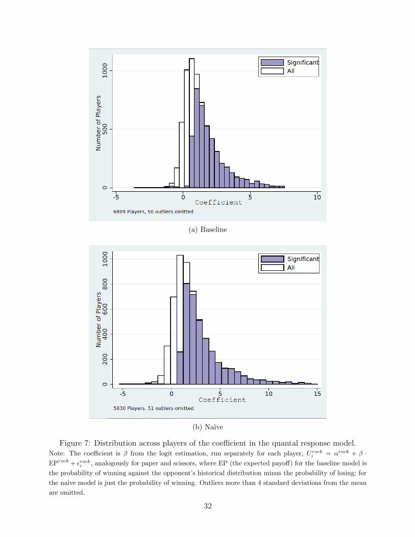
(a) Baseline

(b) Naive

Figure 7: Distribution across players of the coefficient in the quantal response model.Note: The coefficient is β from the logit estimation, run separately for each player, Urock

i = αrock + β ·EProck + εrocki , analogously for paper and scissors, where EP (the expected payoff) for the baseline model is

the probability of winning against the opponent’s historical distribution minus the probability of losing; for

the naive model is just the probability of winning. Outliers more than 4 standard deviations from the mean

are omitted.

32

6 Likelihood comparisonWhich is a better model of player behavior, the discrete “if it is the k1 throw, play it”

or the more continuous “if its k1 payoff is higher, play it with higher probability”? Since

the strategies are similar, if players were using one there would still be some evidence for

the other, so we use a likelihood test to see which model better fits players’ behavior. To

facilitate the comparison, we estimate a “level-k1” model – the level-k model with no k2 –

which also has three independent parameters.38

As in Section 4.5, if we assume that one of two models, level-k1 (LK) and quantal response

(QR), generated the data and have a flat prior over which it was, then according to Bayes

theorem, the probability that it was quantal response is

P (QR | data) =P (data | QR)

P (data | LK) + P (data | QR). (2)

We do this calculation for both the standard level-k and the naive level-k (which we compare

to an analogous naive QR model.)

Figure 8 plots the distribution of this probability across players. For the baseline strate-

gies, level-k and quantal response are evenly matched. For 55.7% of players the quantal

response is a better model; more interestingly, there are substantial numbers of players both

to the left of .05 and to the right of .95. For 1,193 players (17.88%) the level-k1 model is a

statistically better fit and for 1,180 players (17.68%) the quantal response is a statistically

better fit. This suggests some players’ focus more on whether the throw has the highest

expected return (k1) and others players respond more to the level of the expected return

(quantal response). For the naive strategies, the models do about equally well in the over-

all population, but for players whose play is significantly more consistent with one of the

models, they seem to act on whether a throw is most likely to win rather than to have their

play probability be increasing in the probability of winning: for 26.41% of players the naive

level-k1 model is a statistically better fit and for 12.25% of players the naive quantal response

is a statistically better fit.

We do not have any demographic information on players to look at who tends to use

which type of strategy.39 However we can look at whether the number of games they play

or their coefficients estimated from the two models predict which model is a better fit.

Table 13 presents this analysis, separately for all players and those for whom one model

was a significantly better fit. Players who play more games tend to favor the level-k model.

38Models with additional parameters have more flexibility to fit data better even when the underlyingmodel is no better. We find little evidence of k2 and using a k1 model avoids choosing how much to penalizethe level-k model for the additional parameter.

39This would be an interesting dimension for future work to explore.

33

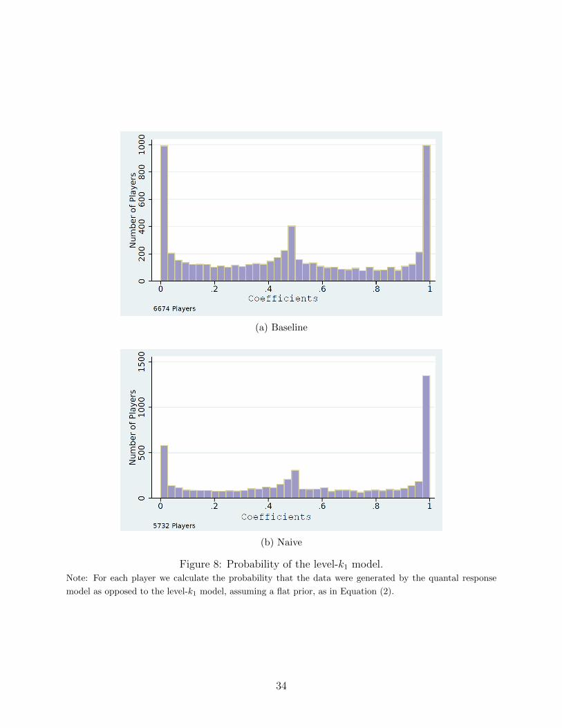
(a) Baseline

(b) Naive

Figure 8: Probability of the level-k1 model.Note: For each player we calculate the probability that the data were generated by the quantal response

model as opposed to the level-k1 model, assuming a flat prior, as in Equation (2).

34

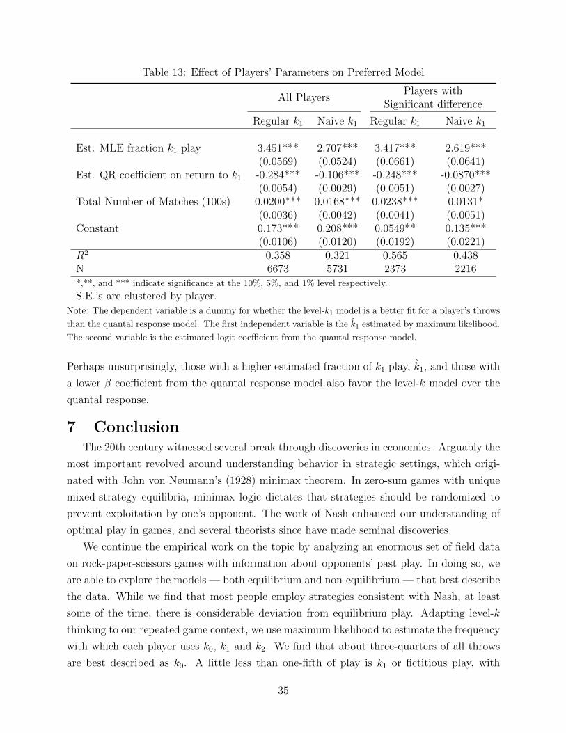
Table 13: Effect of Players’ Parameters on Preferred Model

All PlayersPlayers with

Significant difference

Regular k1 Naive k1 Regular k1 Naive k1

Est. MLE fraction k1 play 3.451*** 2.707*** 3.417*** 2.619***(0.0569) (0.0524) (0.0661) (0.0641)

Est. QR coefficient on return to k1 -0.284*** -0.106*** -0.248*** -0.0870***(0.0054) (0.0029) (0.0051) (0.0027)

Total Number of Matches (100s) 0.0200*** 0.0168*** 0.0238*** 0.0131*(0.0036) (0.0042) (0.0041) (0.0051)

Constant 0.173*** 0.208*** 0.0549** 0.135***(0.0106) (0.0120) (0.0192) (0.0221)

R2 0.358 0.321 0.565 0.438N 6673 5731 2373 2216*,**, and *** indicate significance at the 10%, 5%, and 1% level respectively.

S.E.’s are clustered by player.

Note: The dependent variable is a dummy for whether the level-k1 model is a better fit for a player’s throws

than the quantal response model. The first independent variable is the k1 estimated by maximum likelihood.

The second variable is the estimated logit coefficient from the quantal response model.

Perhaps unsurprisingly, those with a higher estimated fraction of k1 play, k1, and those with

a lower β coefficient from the quantal response model also favor the level-k model over the

quantal response.

7 ConclusionThe 20th century witnessed several break through discoveries in economics. Arguably the

most important revolved around understanding behavior in strategic settings, which origi-

nated with John von Neumann’s (1928) minimax theorem. In zero-sum games with unique

mixed-strategy equilibria, minimax logic dictates that strategies should be randomized to

prevent exploitation by one’s opponent. The work of Nash enhanced our understanding of

optimal play in games, and several theorists since have made seminal discoveries.

We continue the empirical work on the topic by analyzing an enormous set of field data

on rock-paper-scissors games with information about opponents’ past play. In doing so, we

are able to explore the models — both equilibrium and non-equilibrium — that best describe

the data. While we find that most people employ strategies consistent with Nash, at least

some of the time, there is considerable deviation from equilibrium play. Adapting level-k

thinking to our repeated game context, we use maximum likelihood to estimate the frequency

with which each player uses k0, k1 and k2. We find that about three-quarters of all throws

are best described as k0. A little less than one-fifth of play is k1 or fictitious play, with

35

k2 play accounting for less than one-tenth of play. Interestingly, we find that most players

are mixing over at least two levels of reasoning. A model where players focus on winning,

without worrying about losing, suggests similar levels for each strategy and is a better fit for

most players. Since players mix across levels, we explore when they are most likely to play

k1. We find that consistency with k1 is increased when the expected return to k1 is higher.

We also explore the quantal response model. Our adapted version of quantal response

has players paying attention to the expected return to each strategy. We find that a one

standard deviation increase in expected return increases the probability of a throw by 7.3

percentage points. In addition, for about a fifth of players the quantal response model fits

significantly better than the level-k model, but for another one-fifth the level-k model fits

significantly better. It seems that some players focus on the levels of the expected returns,

while others focus on which throw has the highest expected return.

There are several limitations to our analysis, which would be interesting to explore in

future work. Examining play beyond the first throw could shed light on convergence of

strategies within a match. Our dataset does not include demographic information on the

players, so we could not analyze the interaction between strategies and player characteristics.

The differences in strategic choices, though, lead to additional questions: who are the players

who employ more advanced strategies, and why? Finally, there are other simple games that

may lend themselves better to level-k models, including many variants of rock-paper-scissors

with more strategies available to the players and with different payoff structures.

Beyond theory testing, we draw several methodological lessons. First, while our setting is

very different from the single-shot games for which that level-k theory was initially developed,

our finding that players mix across strategies raises questions for experiments that attempt

to categorize players as a k-type based on only a few instances of play. Second, with large

data sets, subtle differences in theoretical predictions can be tested with meaningful power.

As the internet continues to provide unique opportunities for such large-scale data, we hope

that our study can serve as a starting point for future explorations of behavior in both

strategic and non-strategic settings.

36

Appendix to Behavior in Strategic Settings: Evidence from a MillionRock-Paper-Scissors Games

A Proof of Proposition 1We formalize the process of playing rock-papers-scissors over Facebook as a sequence of

best-of-three matches described by the game Γ nested inside a larger game Γ, which includes

the matching process that pairs the players. We do not specify the matching process, as

it turns out that it does not matter and the following holds for any matching process.40

Players may exit the game (and exit may not be random) after any subgame, but not in the

middle of one. All players have symmetric payoffs and discount factor δ across subgames.

Our results are similar to Wooders and Shachat (2001) for two-outcome games.

Each nested game Γ is a “best-of-three” match of rock-paper-scissors played in rounds,

which we will call “throws.” For each throw, both players simultaneously choose actions

a ∈ A = {r, p, s} and the outcome for each player is a win, loss, or tie; r beats s, s beats p,

and p beats r. A player wins Γ by winning two throws. The winner of Γ receives a pay-off

of 1 and the loser gets -1. Note that Γ is zero-sum. Therefore, at any stage of Γ the sum

across players of all future discounted payoffs is zero.

Each match consists of at least two throws. Because of the possibility of ties, there is no

limit on the length of a match. Let

Kl = A2 × A2 . . .× A2︸ ︷︷ ︸l times

be the set of all possible sequences of l throws by two players. Let K l ⊂ Kl be the set of

possible complete matches of length l: sequences of throw pairs such that no player had 2

wins after l − 1 throws, but a player had two wins after the lth throw. Let K = ∪K l be the

set of possible complete matches of any length. Let K l ⊂ Kl be the set of possible incomplete

matches of length l: sequences of throw pairs such that no player has 2 wins.

A player’s overall history after playing t matches is the sequence of match histories for

all matches he has played,

hti ∈ H t = K ×K . . .×K︸ ︷︷ ︸t times

.

Let H−i denote the history of all players in the pool other than i. Players may not observe

their opponents’ exact histories. Instead a player observes some public summary information

of his opponent’s history. Let f : H t → St ∀t be the function that maps histories into

summary information. Denote by st an element of St.

40In the actual game players could challenge a specific player to a game or be matched by the software tosomeone else who was looking for an opponent.

37

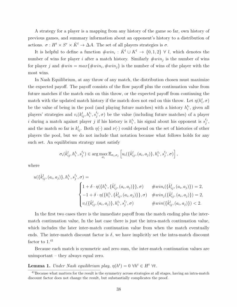
A strategy for a player is a mapping from any history of the game so far, own history of

previous games, and summary information about an opponent’s history to a distribution of

actions. σ : H t × Sr × K l → ∆A. The set of all players strategies is σ.

It is helpful to define a function #wini : K l ∪ K l → {0, 1, 2} ∀ l, which denotes the

number of wins for player i after a match history. Similarly #winj is the number of wins

for player j and #win = max{#wini,#winj} is the number of wins of the player with the

most wins.

In Nash Equilibrium, at any throw of any match, the distribution chosen must maximize

the expected payoff. The payoff consists of the flow payoff plus the continuation value from

future matches if the match ends on this throw, or the expected payoff from continuing the

match with the updated match history if the match does not end on this throw. Let η(hti, σ)

be the value of being in the pool (and playing future matches) with a history htii , given all

players’ strategies and vi(klij, h

tii , s

tjj , σ) be the value (including future matches) of a player

i during a match against player j if his history is htii , his signal about his opponent is stjj ,

and the match so far is klij. Both η(·) and ν(·) could depend on the set of histories of other

players the pool, but we do not include that notation because what follows holds for any

such set. An equilibrium strategy must satisfy

σi(klij, h

tii , s

tjj ) ∈ arg max

σiEσi,σj

[ui({klij, (ai, aj)}, h

tii , s

tjj , σ)

],

where

u({klij, (ai, aj)}, htii , s

tjj , σ) =

1 + δ · η({htii , {klij, (ai, aj)}}, σ) #wini({klij, (ai, aj)}) = 2,

−1 + δ · η({htii , {klij, (ai, aj)}}, σ) #winj({klij, (ai, aj)}) = 2,

vi({klij, (ai, aj)}, htii , s

tjj , σ) #win({klij, (ai, aj)}) < 2.

In the first two cases there is the immediate payoff from the match ending plus the inter-

match continuation value, In the last case there is just the intra-match continuation value,

which includes the later inter-match continuation value from when the match eventually

ends. The inter-match discount factor is δ, we have implicitly set the intra-match discount

factor to 1.41

Because each match is symmetric and zero sum, the inter-match continuation values are

unimportant – they always equal zero.

Lemma 1. Under Nash equilibrium play, η(ht) = 0 ∀ht ∈ H t ∀t.41Because what matters for the result is the symmetry across strategies at all stages, having an intra-match

discount factor does not change the result, but substantially complicates the proof.

38

Proof. Suppose that η(hti) 6= 0. If η(hti) < 0, then a player with that history could deviate

to always playing(13, 13, 13

). The player would win half their matches and lose half their

matches and have continuation value 0. If η(hti) > 0, then since Γ is zero sum at every

stage, there must exist hrj such that η(hrj) < 0, which by the same logic cannot happen in

equilibrium.

Since inter-match continuation values are all zero, the intra-match continuation value

is just the probability of eventually winning the match minus the probability of eventu-

ally losing the match. This means that continuation values are zero-sum: vi(kij, hi, sj) =

−vj(kij, hi, sj).The symmetry of the match also implies that, regardless of history, whenever players are

tied for the number of wins in the match, the continuation value going forward is 0 for both

players.

Lemma 2. In Nash equilibrium if #wini(klij) = #winj(k

lij), then vi(k

lij, hi, sj) = vj(k

lij, hj, si) =

0.

Proof. Assume #wini(klij) = #winj(k

lij). Suppose vi(kij, hi, sj) 6= 0. If vi(kij, hi, sj) < 0,

player i has a profitable deviation to play (13, 13, 13) for the remainder of the match and they

will win with probability one-half, giving them a continuation value of zero. Similarly for j.

We therefore have vi(kij, hi, sj) ≥ 0 and vj(klij, hj, si) ≥ 0 for all match histories.

If vi(klij, hi, sj) > 0 then since the match is zero-sum, there must exist an hi, hj such that

vi(klij, hi, f(hj)) < 0 or vj(k

lij, hj, f(hi)) < 0, which contradicts the above result. Similarly

for vj > 0.

Using this result, we can calculate the continuation when i and j do not have an equal

number of wins.

Lemma 3. In Nash equilibrium, if #wini(klij) = 1 and #winj(k

lij) = 0 then vi(k

lij, hi, sj) = 1

2

and vj(klij, hj, si) = −1

2.

Proof. Assume #wini(klij) = 1 and #winj(k

lij) = 0. Suppose vi(k

lij, hi, sj) <

12. This implies

that player i has a profitable deviation to play (13, 13, 13) for the remainder of the match.

Denote by x, the probability that player i wins when play (13, 13, 13). They win, lose, or draw

on the next throw with equal probability; if they win the next throw, they win the match,

if they lose the next throw, they have a 1/2 probability of winning the match and if there is

a draw, they are back in the same situation of having won 1 throw and j has won zero, so

39

they will win with probability x. So

x =1

3︸︷︷︸win this throw

·1 +1

3︸︷︷︸lose this throw

·12

+1

3︸︷︷︸draw this throw

·x,

which implies that player i will win with probability 34

and lose with probability 14, giving

them an intra-match continuation value of 12. Therefore vi(k

lij, hi, sj) ≥ 1

2. Similar logic

guarantees that vj(klij, hj, si) ≥ −1

2.

If vi(klij, hi, sj) >

12

then since the match is zero-sum, there must exist an hi, hj such that

vi(klij, hi, f(hj)) <

12

or vj(klij, hj, f(hi)) < −1

2, which contradicts the above result. Similarly

for vj(klij, hj, si) > −1

2.

Since the number of wins each player has after any history that has not ended the match

is either 0 or 1, Lemmas 2 and 3 encompass all the possible kli,j. We therefore see that the

continuation value depends only on the number of wins each player has

vi(kli,j, hi, sj) = vi(#wini(k

li,j),#winj(k

li,j)).

So, for every kli,j we can calculate ui({klij, (ai, aj)}, htii , s

tjj ) for each own throw and opponent

throw. Figure 9 gives these payoffs for each possible stage in a match. For each of these

stages, it can only be a Nash Equilibrium if each player expects their opponent to play(13, 13, 13

).

A\B R P SR 0,0 -1

2,12

12,-1

2

P 12,-1

20,0 -1

2,12

S -12,12

12,-1

20,0

(a) Start of Match

A\B R P SR 1

2,-1

20,0 1,-1

P 1,-1 12,-1

20,0

S 0,0 1,-1 12,-1

2

(b) A has 1 win, B has zero

A\B R P SR -1

2,12

-1,1 0,0P 0,0 -1

2,12

-1,1S -1,1 0,0 -1

2,12

(c) B has 1 win, A has zero

A\B R P SR 0,0 -1,1 1,-1P 1,-1 0,0 -1,1S -1,1 1,-1 0,0

(d) A has 1 win, B has 1 win

Figure 9: Total payoffs (flow + continuation) for each stage of the match.

40

B Additional Tables

Table 2b: Response to Percent Paper

Opp’s Historical % Throws (%)

Paper Rock Scissors N

0% - 25% 38.88 38.26 22.87 904,00325% - 30% 36.93 39.04 24.03 568,683

30% - 33 13 % 35.95 37.56 26.49 475,438

33 13 % - 37% 35.23 34.39 30.37 888,846

37% - 42% 32.86 29.76 37.39 671,10642% - 100% 29.91 28.03 42.06 1,173,439

Note: Matches are binned by the opponent’s historical percentage paper on first throws. For each range ofopponent’s historical percentage paper, this table shows the distribution of rock, paper, and scissors throwsthe players use.

Table 2c: Response to Percent Scissors

Opp’s Historical % Throws (%)

Paper Rock Scissors N

0% - 25% 39.61 28.05 32.34 1,308,48425% - 30% 37.96 28.07 33.98 730,391

30% - 33 13 % 35.92 29.67 34.41 546,698

33 13 % - 37% 32.85 34.29 32.86 825,972

37% - 42% 28.77 40.99 30.24 513,18542% - 100% 27.24 46.64 26.12 756,785

Note: Matches are binned by the opponent’s historical percentage scissors on first throws. For each rangeof opponent’s historical percentage scissors, this table shows the distribution of rock, paper, and scissorsthrows the players use.

41

Table 3 Extended: Probability of Playing Rock

Covariate Dependent Var: Dummy for Throwing Rock

(1) (2) (3)Opp’s Fraction Paper (first) -0.0403*** -0.0718*** -0.0952***

(0.0021) (0.0056) (0.0087)Opp’s Fraction Scissors (first) 0.2375*** 0.1552*** 0.1377***

(0.0022) (0.0060) (0.0094)Opp’s Fraction Paper (all) 0.0022 0.0249** 0.0032

(0.0032) (0.0088) (0.0138)Opp’s Fraction Scissors (all) 0.0403*** 0.0238* -0.0187

(0.0033) (0.0093) (0.0146)Opp’s Paper Lag 0.0043*** -0.0016 -0.0043*

(0.0007) (0.0015) (0.0019)Opp’s Scissors Lag 0.0142*** 0.0052** -0.0018

(0.0008) (0.0016) (0.0020)Own Fraction Paper (first) -0.0657*** 0.0290*** -0.1092***

(0.0020) (0.0073) (0.0176)Own Fraction Scissors (first) -0.0816*** 0.0013 -0.3216***

(0.0021) (0.0076) (0.0180)Own Fraction Paper (all) -0.0184*** -0.0551*** -0.1408***

(0.0030) (0.0113) (0.0244)Own Fraction Scissors (all) -0.0097** -0.0781*** -0.0691**

(0.0032) (0.0119) (0.0253)Own Paper Lag -0.0015* 0.0121*** 0.0046*

(0.0007) (0.0015) (0.0019)Own Scissors Lag 0.0031*** 0.0094*** -0.0059**

(0.0008) (0.0016) (0.0019)Constant 0.3423*** -0.0190*** 0.0001

(0.0007) (0.0014) (0.0018)R2 0.0184N 4,433,260

Note: This table adds additional variables for a player’s own history to the specification in Table 3.

42

Table 3b: Probability of Playing Paper

Covariate Dependent Var: Dummy for Throwing Paper

(1) (2) (3)Opp’s Fraction Rock (first) 0.2554*** 0.1441*** 0.1249***

(0.0021) (0.0058) (0.0091)Opp’s Fraction Scissors (first) -0.0363*** -0.0648*** -0.1095***

(0.0022) (0.0060) (0.0095)Opp’s Fraction Rock (all) 0.0682*** 0.0109 0.0054

(0.0032) (0.0091) (0.0144)Opp’s Fraction Scissors (all) -0.0079* -0.0090 0.0070

(0.0034) (0.0096) (0.0153)Opp’s Rock Lag 0.0112*** 0.0048** -0.0047*

(0.0007) (0.0016) (0.0020)Opp’s Scissors Lag 0.0037*** -0.0029 -0.0051**

(0.0007) (0.0016) (0.0019)Own Rock Lag -0.0070*** 0.0102*** -0.0046*

(0.0007) (0.0015) (0.0019)Own Scissors Lag 0.0023*** 0.0127*** 0.0012

(0.0007) (0.0015) (0.0019)Constant 0.3365*** -0.0097*** 0.0065***

(0.0006) (0.0014) (0.0018)R2 0.0216N 4,433,260

Note: All coefficients from one regression. See Table 3 for details.

Table 3c: Probability of Playing Scissors

Covariate Dependent Var: Dummy for Throwing Scissors

(1) (2) (3)Opp’s Fraction Paper (first) 0.2395*** 0.1637*** 0.1241***

(0.0022) (0.0061) (0.0095)Opp’s Fraction Rock (first) -0.0541*** -0.0533*** -0.0963***

(0.0021) (0.0057) (0.0090)Opp’s Fraction Paper (all) 0.0326*** -0.0118 -0.0171

(0.0033) (0.0095) (0.0151)Opp’s Fraction Rock (all) -0.0345*** 0.0031 -0.0192

(0.0032) (0.0090) (0.0143)Opp’s Paper Lag 0.0123*** 0.0045** -0.0025

(0.0007) (0.0016) (0.0020)Opp’s Rock Lag 0.0063*** -0.0022 -0.0021

(0.0007) (0.0016) (0.0019)Own Paper Lag 0.0049*** 0.0096*** -0.0085***

(0.0007) (0.0015) (0.0019)Own Rock Lag -0.0052*** 0.0233*** 0.0011

(0.0007) (0.0015) (0.0019)Constant 0.3034*** 0.0000 0.0047**

(0.0006) (0.0014) (0.0018)R2 0.0214N 4,433,260

Note: All coefficients are from one regression. See Table 3 for details.

43

Table 4b: Opponents’ Response to Expected Payoff of Paper

Opponent’s Expected Opponent’s Throw (%) N

Payoff of Paper Paper Rock Scissors

[−1, −0.666] 33.74 34.52 31.74 2,448

[−0.666, −0.333] 36.5 34.06 29.44 11,126

[−0.333, 0] 34.77 33.78 31.45 836,766

[0, 0.333] 34.27 33.38 32.35 1,358,196

[0.333, 0.666] 32.57 34.57 32.86 9,867

Note: See the note on Table 4 for how expected payoff is calculated.

Table 4c: Opponents’ Response to Expected Payoff of Scissors

Opponent’s Expected Opponent’s Throw (%) N

Payoff of Scissors Paper Rock Scissors

[−1, −0.666] 34.24 32.49 33.27 1,659

[−0.666, −0.333] 33.72 34.97 31.31 19,249

[−0.333, 0] 35.46 32.02 32.52 1,041,591

[0, 0.333] 33.6 34.81 31.59 1,139,164

[0.333, 0.666] 31.73 40.02 28.24 16,740

Note: See the note on Table 4 for how expected payoff is calculated.

44

Table 12b: Effect of Expected k2 Payoff on k2-Consistency (OLS)

(1) (2) (3)Payoff from Playing K2 -0.021*** 0.159*** 0.145***

(0.0010) (0.0015) (0.0019)High Opponent Experience 0.005***

(0.0014)Medium Opponent Experience -0.001

(0.0012)K2 Payoff X High Opponent Experience 0.052***

(0.0037)K2 Payoff X Medium Opponent Experience 0.045***

(0.0029)Experienced 0.006***

(0.0011)Exp X Payoff from Playing K2 -0.012** -0.085*** -0.093***

(0.0047) (0.0047) (0.0065)Exp X High Opponent Experience 0.006**

(0.0027)Exp X Medium Opponent Experience 0.008***

(0.0027)Exp X K2 Payoff X High Opponent Experience -0.027**

(0.011)Exp X K2 Payoff X Medium Opponent Experience -0.036***

(0.010)Own Games>100 0.002

(0.0018)Own Games>100 X Payoff from Playing K2 -0.097*** 0.144*** 0.119***

(0.021) (0.013) (0.022)Own Games>100 X High Opponent Experience -0.024***

(0.0025)Own Games>100 X Medium Opponent Experience -0.025***

(0.0031)Own Games>100 X K2 Payoff X High Opponent Experience 0.170***

(0.028)Own Games>100 X K2 Payoff X Medium Opponent Experience 0.180***

(0.033)Player Fixed Effects No Yes YesObservations 4130024 4130024 4130024Adjusted R2 0.000 0.003 0.004

*,**, and *** indicate significance at the 10%, 5%, and 1% level respectively.S.E.’s are clustered by player.

Note: The dependent variable is a dummy for a throw being k2-consistent. ‘k2 Payoff’ equals the opponent’sk1 payoff, as a measure of how much incentive the opponent has to play k1, which increases the payoff to k2.See Table 12 for definitions of the other variables.

45

ReferencesArad, A. and Rubinstein, A. (2012). The 11-20 money request game: A level-k reasoning study. The

American Economic Review, 102(7):3561–3573.

Berger, U. (2005). Fictitious play in 2xn games. Journal of Economic Theory, 120:139–154.

Berger, U. (2007). Brown’s original fictitious play. Journal of Economic Theory, 135:572–578.

Bosch-Domenech, A., Montalvo, J. G., Nagel, R., and Satorra, A. (2002). One, two, (three), infinity,...:

Newspaper and lab beauty-contest experiments. The American Economic Review, 92(5):1687–1701.

Brown, A., Camerer, C., and Lovallo, D. (2012). To review or not to review? Limited strategic thinking at

the movie box office. American Economic Journal: Microeconomics, 4(2):1–26.

Brown, G. W. (1951). Iterative solutions of games by fictitious play. In Koopmans, T., editor, Activity

Analysis of Production and Allocation. New York: Wiley.

Camerer, C. (2003). Behavioral game theory: Experiments in strategic interaction. Princeton University

Press.

Camerer, C., Ho, T.-H., and Chong, J.-K. (2004). A cognitive hierarchy model of games. The Quarterly

Journal of Economics, 119(3):861–898.

Cason, T. N., Friedman, D., and Hopkins, E. (2013). Cycles and instability in a rock–paper–scissors popu-

lation game: a continuous time experiment. Review of Economic Studies, 81(1):112–136.

Chiappori, P.-A., Levitt, S., and Groseclose, T. (2002). Testing mixed-strategy equilibria when players are

heterogeneous: The case of penalty kicks in soccer. American Economic Review, 92(4):1138–1151.

Costa-Gomes, M. and Crawford, V. P. (2006). Cognition and behavior in two-person guessing games: An

experimental study. The American Economic Review, 96(5):1737–1768.

Costa-Gomes, M., Crawford, V. P., and Broseta, B. (2001). Cognition and behavior in normal-form games:

An experimental study. Econometrica, 69(5):1193–1235.

Crawford, V. P. and Iriberri, N. (2007). Fatal attraction: Salience, naivete, and sophistication in experimental

“hide-and-seek” games. The American Economic Review, 97(5):1731–1750.

Facebook (2010). Developer partner case study: Red Bull application.

Frey, B. S. and Meier, S. (2004). Social comparisons and pro-social behavior: Testing” conditional coopera-

tion” in a field experiment. American Economic Review, pages 1717–1722.

Georganas, S., Healy, P. J., and Weber, R. A. (2014). On the persistence of strategic sophistication. Ohio

State Working Paper.

Gillen, B. (2009). Identification and estimation of level-k auctions. Working Paper.

Goldfarb, A. and Xiao, M. (2011). Who thinks about the competition? Managerial ability and strategic

entry in US local telephone markets. The American Economic Review, 101(7):3130–3161.

Hahn, P. R., Goswami, I., and Mela, C. (2014). A bayesian hierarchical model for inferring player strategy

types in a number guessing game. Working Paper.

Hedden, T. and Zhang, J. (2002). What do you think I think you think?: Strategic reasoning in matrix

games. Cognition, 85(1):1–36.

Ho, T.-H., Camerer, C., and Weigelt, K. (1998). Iterated dominance and iterated best response in experi-

mental “p-beauty contests”. The American Economic Review, 88(4):947–969.

46

Hoffman, M., Suetens, S., Gneezy, U., and Nowak, M. A. (2015). An experimental investigation of evolu-

tionary dynamics in the rock-paper-scissors game. Scientific reports, 5.

Houser, D., Keane, M., and McCabe, K. (2004). Behavior in a dynamic decision problem: An analysis of

experimental evidence using a bayesian type classification algorithm. Econometrica, 72(3):781–822.

Kagel, J. H. and Roth, A. E. (1995). The handbook of experimental economics. Princeton university press

Princeton, NJ.

Karlan, D. S. (2005). Using experimental economics to measure social capital and predict financial decisions.

American Economic Review, pages 1688–1699.

Kline, B. (2014). An empirical model of non-equilibrium behavior in games. Working paper.

McFadden, D. (1976). Quantal choice analysis: A survey.

McKelvey, R. D. and Palfrey, T. R. (1995). Quantal response equilibria for normal form games. Games and

economic behavior, 10(1):6–38.

Monderer, D. and Shapley, L. S. (1996). Fictitious play property for games with identical interests. Journal

of Economic Theory, 68(1):258–265.

Mookherjee, D. and Sopher, B. (1994). Learning behavior in an experimental matching pennies game. Games

and Economic Behavior, 7(1):62–91.

Mookherjee, D. and Sopher, B. (1997). Learning and decision costs in experimental constant sum games.

Games and Economic Behavior, 19(1):97–132.

Nagel, R. (1995). Unraveling in guessing games: An experimental study. The American Economic Review,

85(5):1313–1326.

Ostling, R., Wang, J., Chou, E., and Camerer, C. (2011). Testing game theory in the field: Swedish LUPI

lottery games. American Economic Journal: Microeconomics, 3(3):1–33.

Stahl, D. O. (1993). Evolution of smartn players. Games and Economic Behavior, 5(4):604–617.

Stahl, D. O. and Wilson, P. W. (1994). Experimental evidence on players’ models of other players. Journal

of economic behavior & organization, 25(3):309–327.

Stahl, D. O. and Wilson, P. W. (1995). On players’ models of other players: Theory and experimental

evidence. Games and Economic Behavior, 10(1):218–254.

Vogel, C. (2005). Rock, paper, payoff: Child’s play wins auction house an art sale. The New York Times.

April 29.

Walker, M. and Wooders, J. (2001). Minimax play at wimbledon. American Economic Review, pages

1521–1538.

Weber, R. A. (2003). ‘learning’ with no feedback in a competitive guessing game. Games and Economic

Behavior, 44(1):134–144.

Wooders, J. and Shachat, J. M. (2001). On the irrelevance of risk attitudes in repeated two-outcome games.

Games and Economic Behavior, 34(2):342–363.

Wright, J. R. and Leyton-Brown, K. (2017). Predicting human behavior in unrepeated, simultaneous-move

games. Games and Economic Behavior, 106:16–37.

Young, H. P. (1993). The evolution of conventions. Econometrica, 61(1):57–84.

47