Embed Size (px)
Citation preview
Behavior Modes
Meir Kalech
Partially Based on slides of Brian Williams, Luca Console and Peter struss

Outline Last lecture:
1. Generation of tests/probes
2. Measurement Selection
3. Probabilities of Diagnoses
Today’s lecture:
1. Models of correct + faulty behavior
2. Sherlock engine
3. Abductive diagnosis
4. Qualitative models
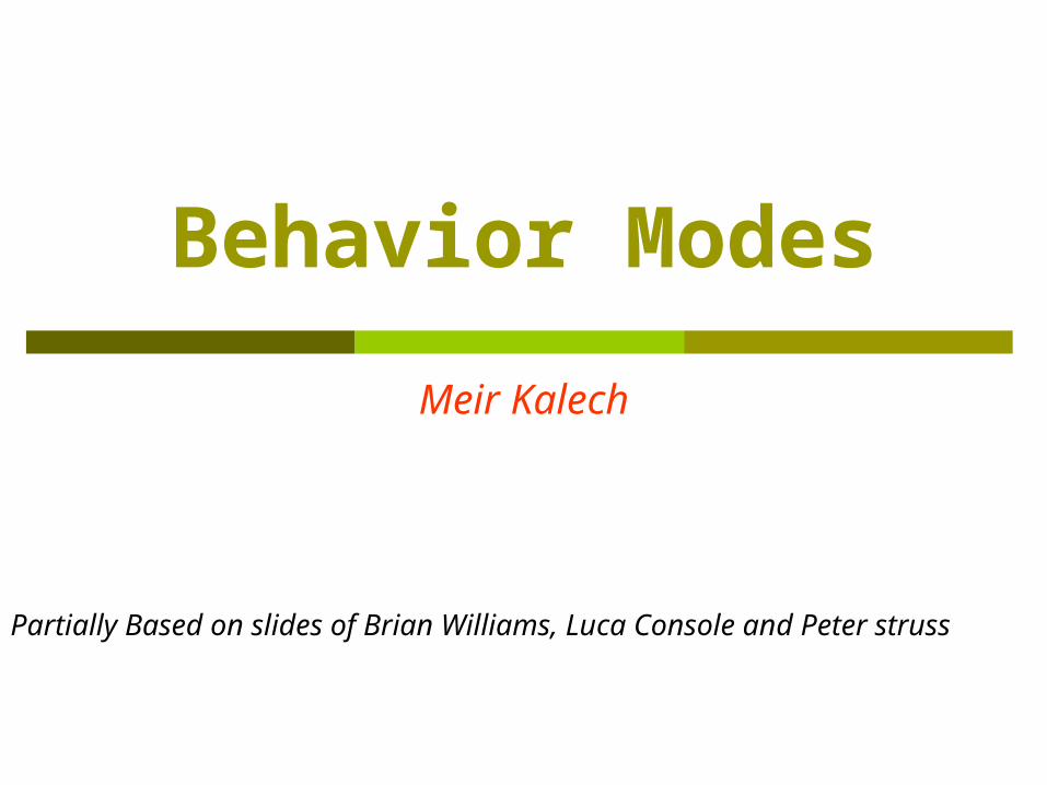
Exploiting models of correct/faulty behaviorInitial proposal: using only models of correct behavior
They are those that are in strict accordance with the goals (easy to acquire, e.g., from design)
But unfortunately they are not always sufficient Need of exploiting also fault models of some form
predictive models [Struss, Dressler, 89] – GDE+[de Kleer, Williams 89] - SHERLOCK
“weak” models of physical impossibility [Friedrich et al. 90]
behavioral models [Console, Torasso, 91]

Diagnosis With Only the Unknown
Inverter(i): G(i): Out(i) = not(In(i)) U(i):
X YA B C0 00
Nominal and Unknown Modes
• Isolates surprises• Doesn’t explain
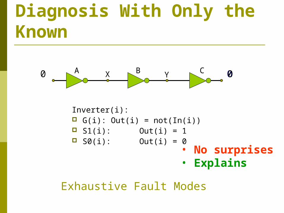
Diagnosis With Only the Known
Inverter(i): G(i): Out(i) = not(In(i)) S1(i): Out(i) = 1 S0(i): Out(i) = 0
X YA B C 00 0
Exhaustive Fault Modes
• No surprises• Explains
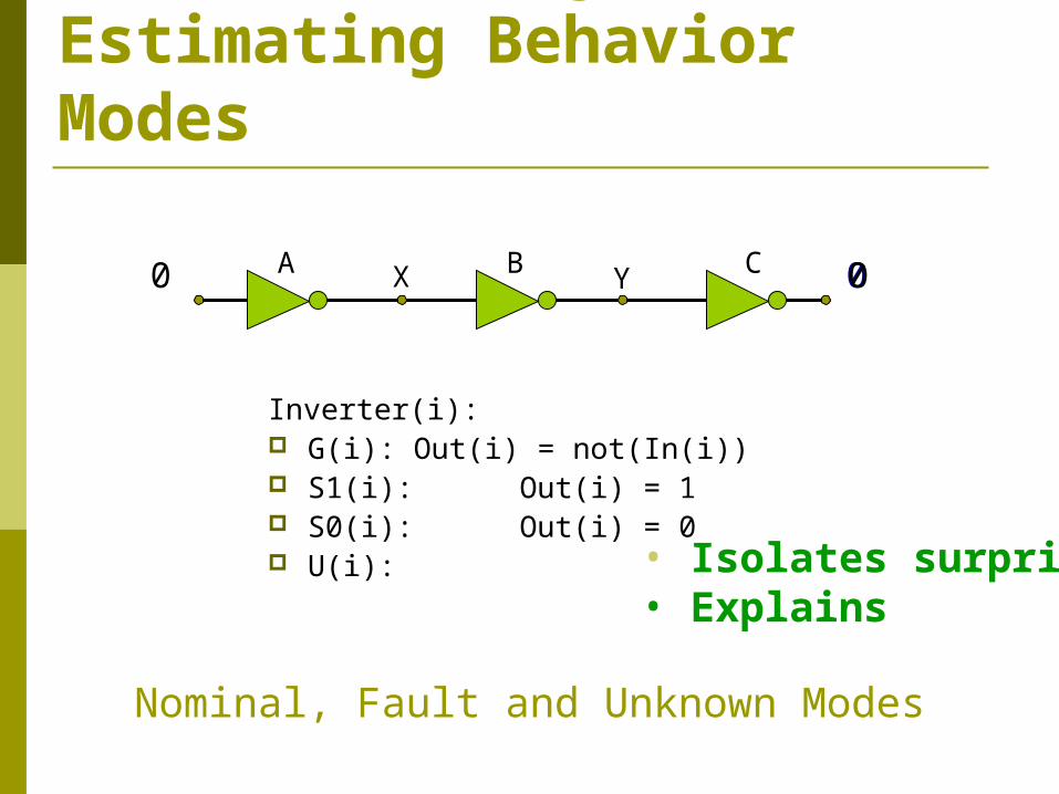
Solution: Diagnosis as Estimating Behavior Modes
Inverter(i): G(i): Out(i) = not(In(i)) S1(i): Out(i) = 1 S0(i): Out(i) = 0 U(i):
X YA B C 00 0
Nominal, Fault and Unknown Modes
• Isolates surprises• Explains

Measurement motivation to use Behavior modes Knowledge of failure modes is important to
decide what measurement to make next. If all faults were equally likely, measuring X or
Y provides equal information. Suppose:
Inverters A and B almost always fail by stuck-at-1. Inverter C almost always fails by stuck at-0.
It is unlikely that inverter A is failing. The likely failures of inverters B and C are
consistent with the symptom

Behavior Modes
• System comprises a (finite) set of components COMPS = { Ci }
• Each Ci has a (finite) set of behavior modes modes(Ci) = { mij
(Ci)}
• E.g.- (unique) correct behavior: ok(Ci)
- (any) faulty behavior: ok(Ci)
- a specific fault: stuck-closed(valvei)
• Behavior mode operating mode (of correct behavior)• E.g. blocking mode of a diode
Definition (Mode Assignment)• COMPS’ COMPS
• MA = {mij(Ci) Ci COMPS’ }
• or MA = Ci COMPS’ mij(Ci)
• MA complete: COMPS’=COMPS
Definition (Mode Assignment)• COMPS’ COMPS
• MA = {mij(Ci) Ci COMPS’ }
• or MA = Ci COMPS’ mij(Ci)
• MA complete: COMPS’=COMPS

Diagnoses as Assignments of Fault Modes
Definition (Diagnosis):• A complete mode assignment MA that is consistent with
the observations: SD MA OBS
Definition (Diagnosis):• A complete mode assignment MA that is consistent with
the observations: SD MA OBS
Definition (Mode Assignment)• COMPS’ COMPS
• MA = {mij(Ci) Ci COMPS’ }
• or MA = Ci COMPS’ mij(Ci)
• MA complete: COMPS’=COMPS
Definition (Mode Assignment)• COMPS’ COMPS
• MA = {mij(Ci) Ci COMPS’ }
• or MA = Ci COMPS’ mij(Ci)
• MA complete: COMPS’=COMPS

Yet Another Simple Example
Battery
RLight
HLight
Starter
Head lights work Starter and rear light don’t Obvious diagnosis:
Starter and rear light are broken
Head lights work Starter and rear light don’t Obvious diagnosis:
Starter and rear light are broken
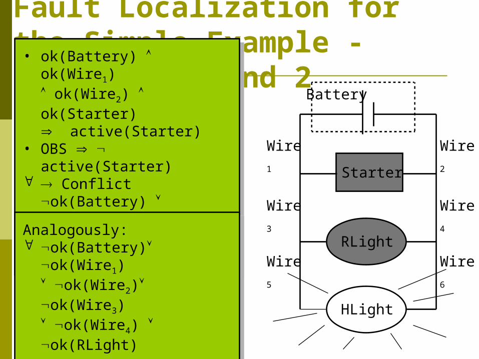
Fault Localization for the Simple Example - Conflicts 1 and 2
Battery
RLight
HLight
Starter
• ok(Battery) ok(Wire1) ok(Wire2) ok(Starter) active(Starter)
• OBS active(Starter) Conflict
ok(Battery) ok(Wire1) ok(Wire2) ok(Starter)
• ok(Battery) ok(Wire1) ok(Wire2) ok(Starter) active(Starter)
• OBS active(Starter) Conflict
ok(Battery) ok(Wire1) ok(Wire2) ok(Starter)
Wire1
Wire3
Wire5
Wire2
Wire4
Wire6Analogously: ok(Battery) ok(Wire1)
ok(Wire2) ok(Wire3) ok(Wire4) ok(RLight)
Analogously: ok(Battery) ok(Wire1)
ok(Wire2) ok(Wire3) ok(Wire4) ok(RLight)

Fault Localization for the Simple Example - Conflicts 3 and 4
Battery
RLight
HLight
Starter
• lit(HLight) ok(HLight) ok(Wire5) ok(Wire6) ok(RLight) lit(RLight)
• OBS lit(RLight) Conflict
ok(HLight) ok(Wire5)
ok(Wire6) ok(RLight)
• lit(HLight) ok(HLight) ok(Wire5) ok(Wire6) ok(RLight) lit(RLight)
• OBS lit(RLight) Conflict
ok(HLight) ok(Wire5)
ok(Wire6) ok(RLight)
Wire1
Wire3
Wire5
Wire2
Wire4
Wire6Analogously: ok(HLight) ok(Wire5)
ok(Wire6) ok(Wire3) ok(Wire4) ok(Starter)
Analogously: ok(HLight) ok(Wire5)
ok(Wire6) ok(Wire3) ok(Wire4) ok(Starter)
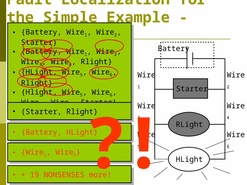
Fault Localization for the Simple Example - Hitting Sets
Battery
RLight
HLight
Starter
Wire1
Wire3
Wire5
Wire2
Wire4
Wire6
• {Battery, Wire1, Wire2, Starter}• {Battery, Wire1, Wire2, Wire3,
Wire4, Rlight}
• {HLight, Wire5, Wire6, Rlight} • {Hlight, Wire5, Wire6, Wire3,
Wire4, Starter}
• {Battery, Wire1, Wire2, Starter}• {Battery, Wire1, Wire2, Wire3,
Wire4, Rlight}
• {HLight, Wire5, Wire6, Rlight} • {Hlight, Wire5, Wire6, Wire3,
Wire4, Starter}
• {Starter, Rlight}• {Starter, Rlight}
• {Battery, HLight}• {Battery, HLight}
• {Wire1, Wire5}• {Wire1, Wire5}
• + 19 NONSENSES more!• + 19 NONSENSES more!!?

What Makes Most of the Fault Localizations Implausible?
Battery
RLight
HLight
Starter
Wire1
Wire3
Wire5
Wire2
Wire4
Wire6
• If the battery were broken, the headlights would not be lit
• Broken headlights cannot be lit Knowledge about faults can
reduce the set of fault localizations
• If the battery were broken, the headlights would not be lit
• Broken headlights cannot be lit Knowledge about faults can
reduce the set of fault localizations
• {Starter, Rlight}• {Starter, Rlight}
• {Battery, HLight}• {Battery, HLight}
• {Wire1, Wire5}• {Wire1, Wire5}
• + 19 more!• + 19 more!!?
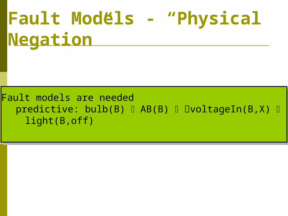
Fault Models - “Physical Negation”
Fault models are neededpredictive: bulb(B) AB(B) voltageIn(B,X) light(B,off)
Fault models are neededpredictive: bulb(B) AB(B) voltageIn(B,X) light(B,off)

Outline Last lecture:
1. Generation of tests/probes
2. Measurement Selection
3. Probabilities of Diagnoses
Today’s lecture:
1. Models of correct + faulty behavior
2. Sherlock engine
3. Abductive diagnosis
4. Qualitative models

Search Guided by Probabilities: SHERLOCK ([de Kleer- Williams 89])
• Basic Idea: Search for the most probable explanations of the observations
• Fault models for each component (type)• Possible: unknown fault mode
• Modes have prior probability Mode assignments have a probability • SHERLOCK: best first search for consistent mode assignments• termination criteria
• Basic Idea: Search for the most probable explanations of the observations
• Fault models for each component (type)• Possible: unknown fault mode
• Modes have prior probability Mode assignments have a probability • SHERLOCK: best first search for consistent mode assignments• termination criteria

Leading Diagnoses Complexity of diagnoses space:
n-#components, m-#modesGDE 2n SHERLOCK: mn
To reduce the high complexity, generate only leading diagnoses:
1. Diagnoses are those with the highest probabilities.2. No more than k1 (=5) leading diagnoses.3. Candidates with probability less than 1/k2(=100)
of the best diagnosis are not considered4. The diagnoses need not include more than k3
(=0.75) of the total probability mass of the candidates.

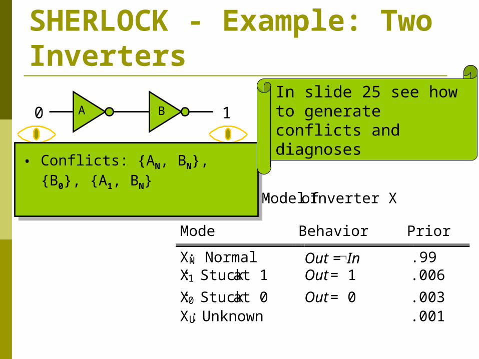
SHERLOCK - Example: Two Inverters
A B0 1
Model of Inverter X
Mode Behavior Prior
XN: Normal Out =In .99X1: Stuck at 1 Out = 1 .006
X0: Stuck at 0 Out = 0 .003XU: Unknown .001
SHERLOCK - Example: Two Inverters
A B0 1
Model of Inverter X
Mode Behavior Prior
XN: Normal Out =In .99X1: Stuck at 1 Out = 1 .006
X0: Stuck at 0 Out = 0 .003XU: Unknown .001
• Conflicts: {AN, BN}, {B0}, {A1, BN}
• Conflicts: {AN, BN}, {B0}, {A1, BN}
In slide 25 see how to generate conflicts and diagnoses

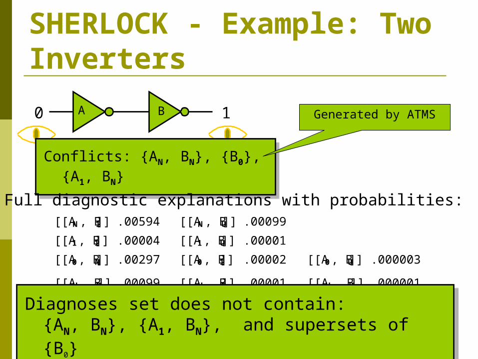
SHERLOCK - Example: Two Inverters
A B0 1
• Conflicts: {AN, BN}, {B0}, {A1, BN}
• Conflicts: {AN, BN}, {B0}, {A1, BN}
• Inspired by GDE + modes• Diagnosis is an explanation: SDMAOBS ┴ , where
MA=CiCOMPSmij(Ci), (rather than a set of faulty components)
• I.E., the diagnosis set contains all the combinations of the components’ modes except of conflicts.
• Inspired by GDE + modes• Diagnosis is an explanation: SDMAOBS ┴ , where
MA=CiCOMPSmij(Ci), (rather than a set of faulty components)
• I.E., the diagnosis set contains all the combinations of the components’ modes except of conflicts.
SHERLOCK - Example: Two Inverters
A B0 1
[[AN , B1]] .00594 [[AN , BU]] .00099
[[A1 , B1]] .00004 [[A1 , BU]] .00001
[[A0 , BN]] .00297 [[A0 , B1]] .00002 [[A0 , BU]] .000003
[[AU , BN]] .00099 [[AU , B1]] .00001 [[AU , BU]] .000001
Conflicts: {AN, BN}, {B0}, {A1, BN}Conflicts: {AN, BN}, {B0}, {A1, BN}
Diagnoses set does not contain:{AN, BN}, {A1, BN}, and supersets of {B0}
Diagnoses set does not contain:{AN, BN}, {A1, BN}, and supersets of {B0}
Generated by ATMS
Full diagnostic explanations with probabilities:

SHERLOCK - Example: Two Inverters
A B0 1
[[AN , B1]] .00594 [[AN , BU]] .00099
[[A1 , B1]] .00004 [[A1 , BU]] .00001
[[A0 , BN]] .00297 [[A0 , B1]] .00002 [[A0 , BU]] .000003
[[AU , BN]] .00099 [[AU , B1]] .00001 [[AU , BU]] .000001
Conflicts: {AN, BN}, {B0}, {A1, BN}Conflicts: {AN, BN}, {B0}, {A1, BN}
Generated by ATMS
Full diagnostic explanations with probabilities:
• Exhaustive search impossible• Perform best first search
• Exhaustive search impossible• Perform best first search

SHERLOCK - Example: Search Strategy
{ } 1.0 1
{An,B1} .00594 5
{An,Bn} .98010 3 x
{An,B0} .00297 8 x
{An,Bu} .00099
{A0,Bn} .00297 9
{A0,B1} .00002
{A0,B0} .000009 x{A0,Bu} .000003
{A1,B1} .00004
{A1,Bn} .00594 6 x
{A1,B0} .00002 x
{A1,Bu} .00001
{An} .99 2
{A1} .006 4
{A0} .003 7
{Au} .001
0 1A B
Legend:
x inconsistent
Legend:
x inconsistentMA Probability Step # Consistent ?
Generate the next explanation with the highest probability
Generate the next explanation with the highest probability
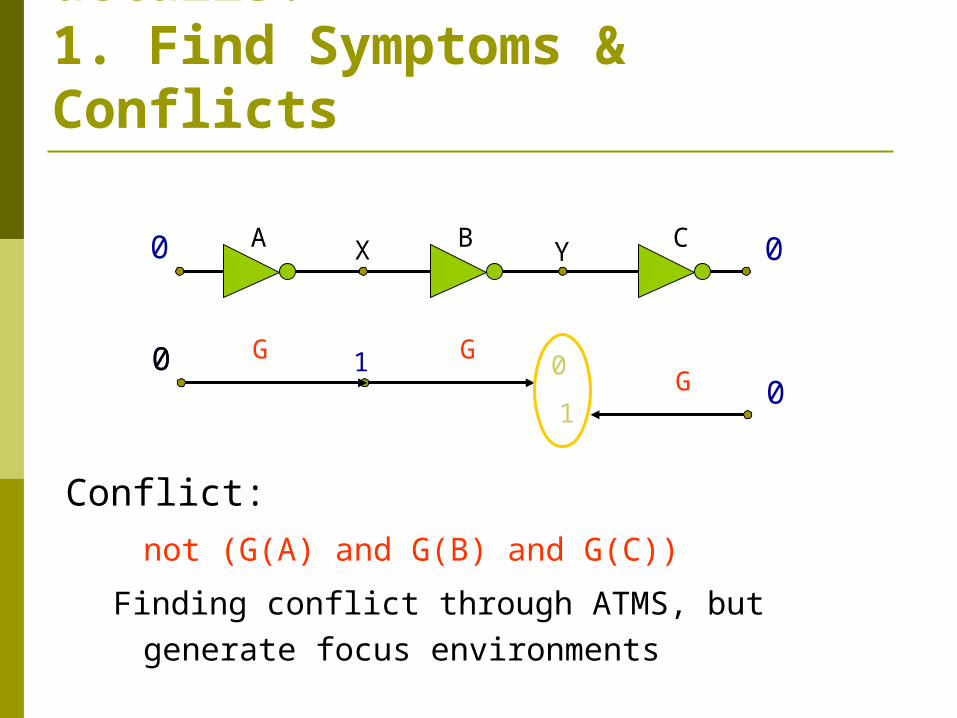
SHERLOCK, Process in details:1. Find Symptoms & Conflicts
Conflict:
not (G(A) and G(B) and G(C))
Finding conflict through ATMS, but generate focus environments
X YA B C0 0
1 0G G
G0
01
0
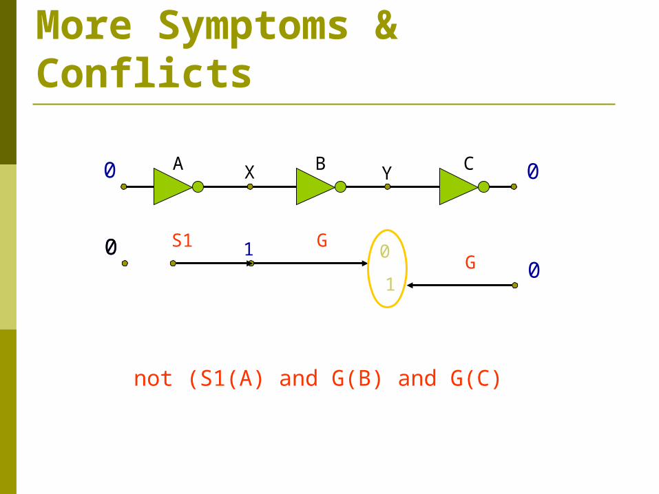
More Symptoms & Conflicts
not (S1(A) and G(B) and G(C)
X YA B C0 0
1 0S1 G
G0
01
0
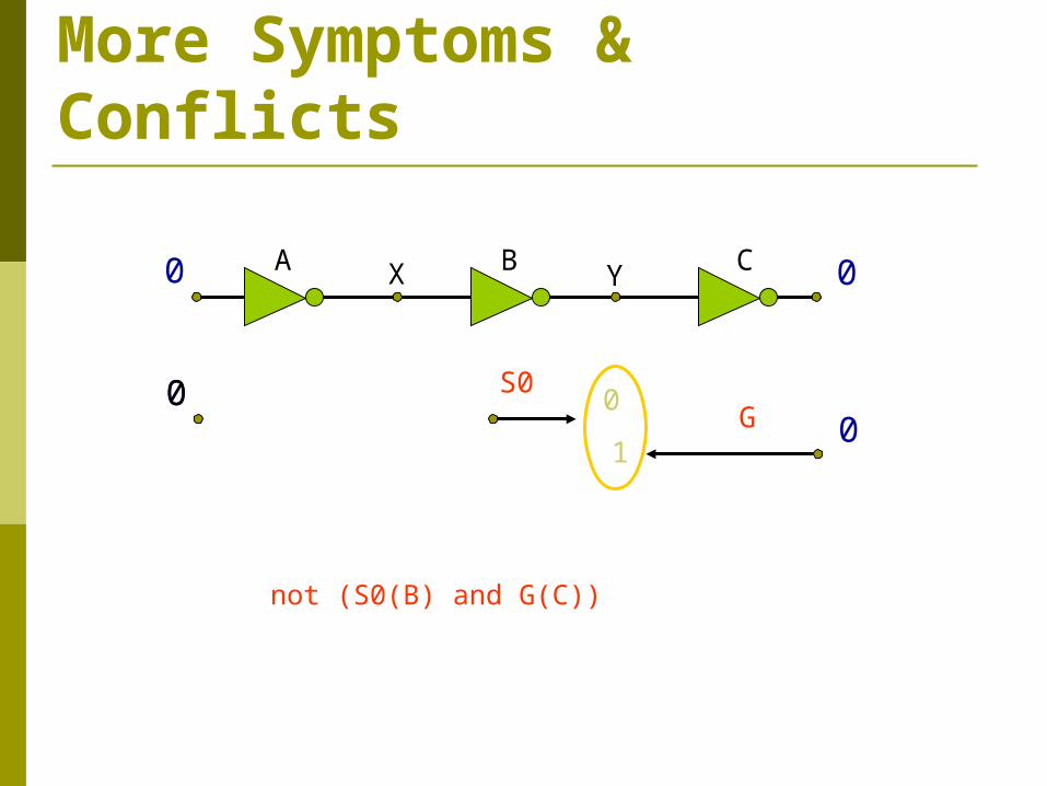
not (S0(B) and G(C))
X YA B C0 0
0S0
G0
01
More Symptoms & Conflicts
0
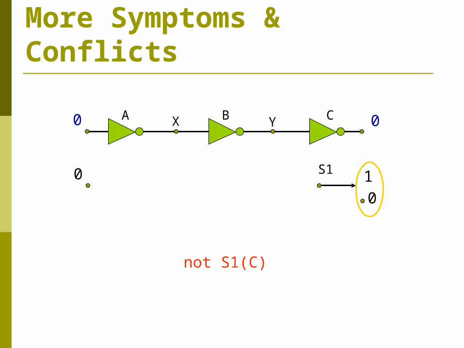
not S1(C)
X YA B C0 0
1S10
0
More Symptoms & Conflicts

All Minimal Conflicts < S1(C) >
< S0(B), G(C) >
< S1(A), G(B), G(C) >
< G(A), G(B), G(C) >
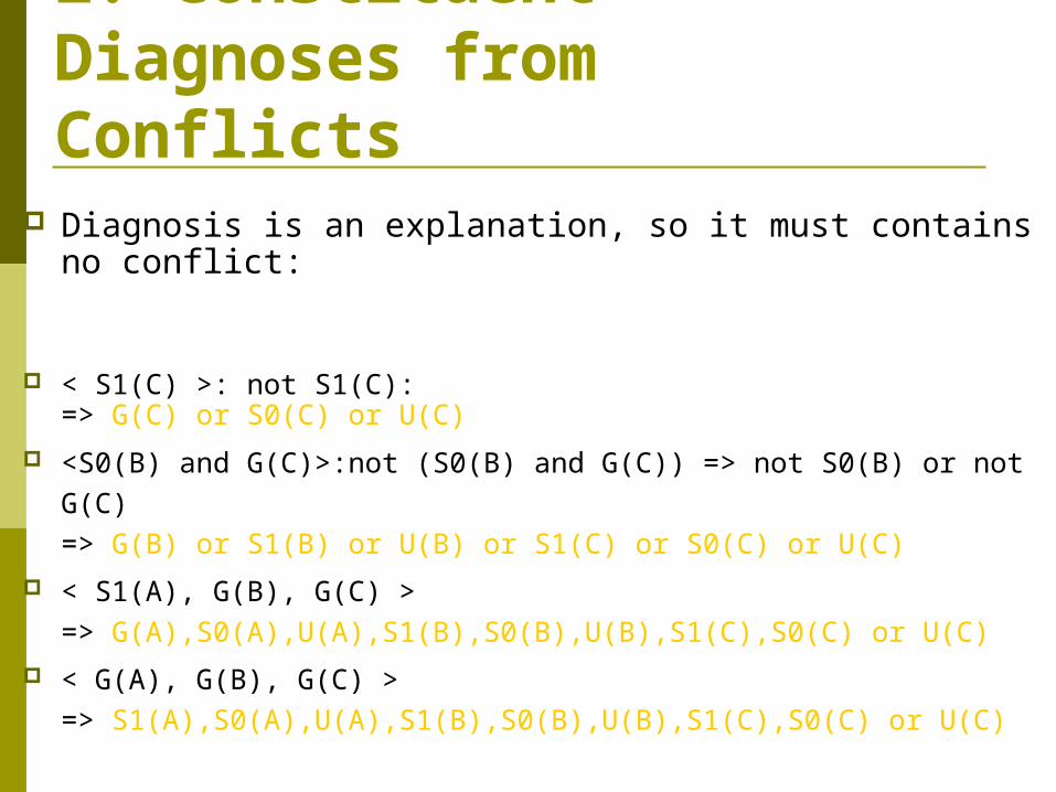
2. Constituent Diagnoses from Conflicts
Diagnosis is an explanation, so it must contains no conflict:
< S1(C) >: not S1(C):=> G(C) or S0(C) or U(C)
<S0(B) and G(C)>:not (S0(B) and G(C)) => not S0(B) or not G(C) => G(B) or S1(B) or U(B) or S1(C) or S0(C) or U(C)
< S1(A), G(B), G(C) >=> G(A),S0(A),U(A),S1(B),S0(B),U(B),S1(C),S0(C) or U(C)
< G(A), G(B), G(C) >=> S1(A),S0(A),U(A),S1(B),S0(B),U(B),S1(C),S0(C) or U(C)

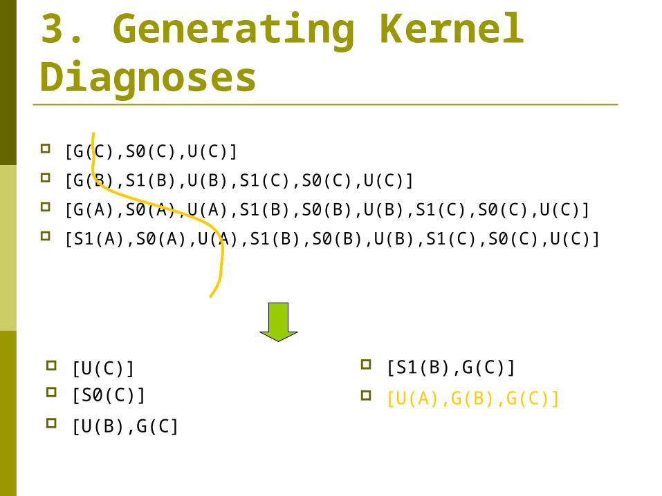
3. Generating Kernel Diagnoses
[U(C)]
[G(C),S0(C),U(C)]
[G(B),S1(B),U(B),S1(C),S0(C),U(C)]
[G(A),S0(A),U(A),S1(B),S0(B),U(B),S1(C),S0(C),U(C)]
[S1(A),S0(A),U(A),S1(B),S0(B),U(B),S1(C),S0(C),U(C)]

[U(C)] [S0(C)]
[G(C),S0(C),U(C)]
[G(B),S1(B),U(B),S1(C),S0(C),U(C)]
[G(A),S0(A),U(A),S1(B),S0(B),U(B),S1(C),S0(C),U(C)]
[S1(A),S0(A),U(A),S1(B),S0(B),U(B),S1(C),S0(C),U(C)]
3. Generating Kernel Diagnoses

[U(C)] [S0(C)]
[U(B),G(C)]
[G(C),S0(C),U(C)]
[G(B),S1(B),U(B),S1(C),S0(C),U(C)]
[G(A),S0(A),U(A),S1(B),S0(B),U(B),S1(C),S0(C),U(C)]
[S1(A),S0(A),U(A),S1(B),S0(B),U(B),S1(C),S0(C),U(C)]
3. Generating Kernel Diagnoses

[U(C)] [S0(C)]
[U(B),G(C)]
[G(C),S0(C),U(C)]
[G(B),S1(B),U(B),S1(C),S0(C),U(C)]
[G(A),S0(A),U(A),S1(B),S0(B),U(B),S1(C),S0(C),U(C)]
[S1(A),S0(A),U(A),S1(B),S0(B),U(B),S1(C),S0(C),U(C)]
[S1(B),G(C)]
3. Generating Kernel Diagnoses
[U(C)] [S0(C)]
[U(B),G(C]
[S1(B),G(C)]
[U(A),G(B),G(C)]
[G(C),S0(C),U(C)]
[G(B),S1(B),U(B),S1(C),S0(C),U(C)]
[G(A),S0(A),U(A),S1(B),S0(B),U(B),S1(C),S0(C),U(C)]
[S1(A),S0(A),U(A),S1(B),S0(B),U(B),S1(C),S0(C),U(C)]
3. Generating Kernel Diagnoses
[U(C)] [S0(C)]
[U(B),G(C]
[S1(B),G(C)]
[U(A),G(B),G(C)]
[S0(A),G(B),G(C)]
[G(C),S0(C),U(C)]
[G(B),S1(B),U(B),S1(C),S0(C),U(C)]
[G(A),S0(A),U(A),S1(B),S0(B),U(B),S1(C),S0(C),U(C)]
[S1(A),S0(A),U(A),S1(B),S0(B),U(B),S1(C),S0(C),U(C)]
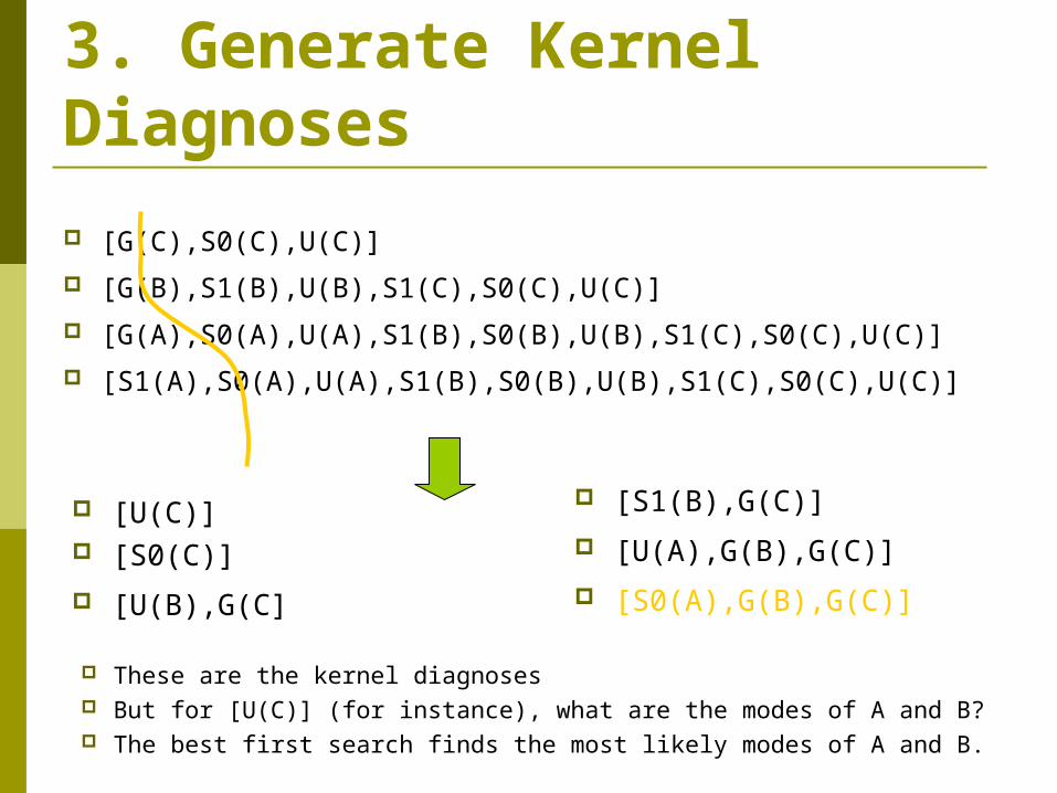
3. Generate Kernel Diagnoses
These are the kernel diagnoses But for [U(C)] (for instance), what are the modes of A and B? The best first search finds the most likely modes of A and B.

Candidate Initial (prior) Probabilities
p(c) p(m)mc
A B C
p(G) .99 .99 .99
p(S1) .008 .008 .001
p(S0) .001 .001 .008
p(U) .001 .001 .001

No observations With no observations Sherlock finds the single leading diagnosis
The unfocused Sherlock finds 43 diagnoses

Input I=0 Sherlock computes the following environments:
The focused Sherlock finds no label for X=0 as it does not hold in the single leading diagnosis.
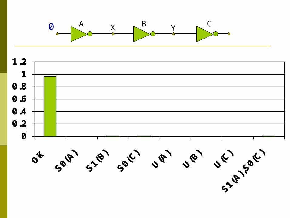
00.20.40.60.8
11.2
X YA B C0
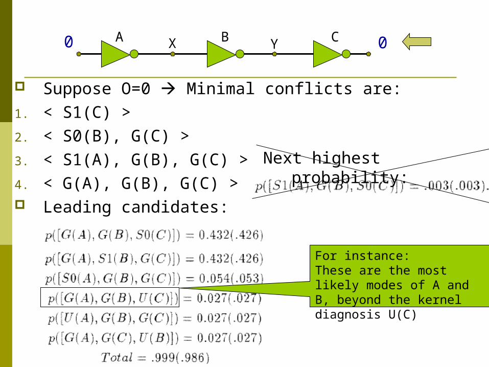
Suppose O=0 Minimal conflicts are:1. < S1(C) >2. < S0(B), G(C) >3. < S1(A), G(B), G(C) >4. < G(A), G(B), G(C) > Leading candidates:
X YA B C0 0
Next highest probability:
For instance:These are the most likely modes of A and B, beyond the kernel diagnosis U(C)
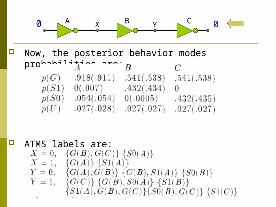
Now, the posterior behavior modes probabilities are:
ATMS labels are:
X YA B C0 0
0
0.1
0.2
0.3
0.4
0.5
X YA B C0 0
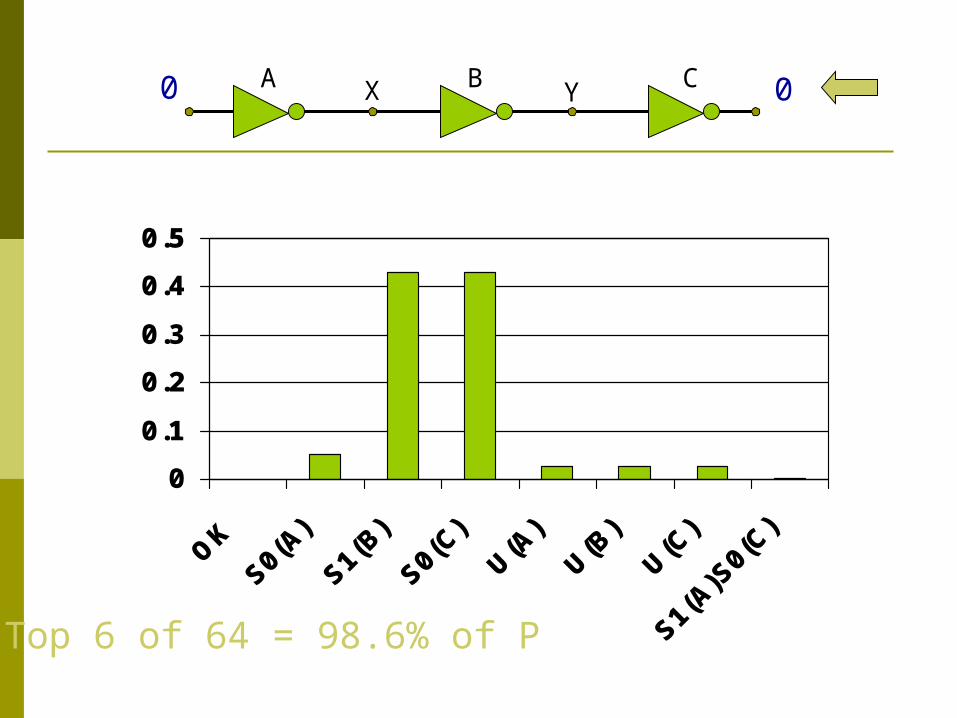
Top 6 of 64 = 98.6% of P
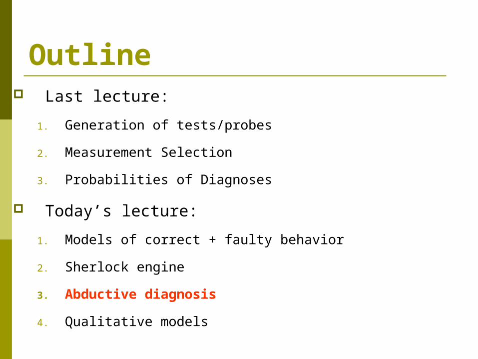
Outline Last lecture:
1. Generation of tests/probes
2. Measurement Selection
3. Probabilities of Diagnoses
Today’s lecture:
1. Models of correct + faulty behavior
2. Sherlock engine
3. Abductive diagnosis
4. Qualitative models
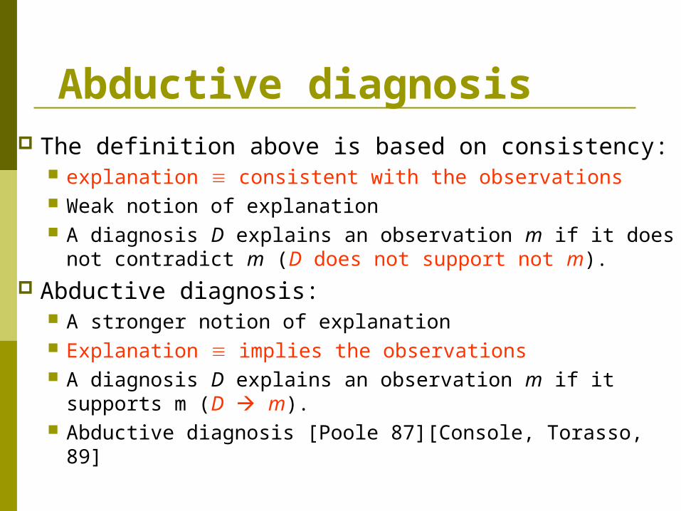
Abductive diagnosis The definition above is based on consistency:
explanation consistent with the observations Weak notion of explanation A diagnosis D explains an observation m if it does not
contradict m (D does not support not m). Abductive diagnosis:
A stronger notion of explanation Explanation implies the observations A diagnosis D explains an observation m if it supports
m (D m). Abductive diagnosis [Poole 87][Console, Torasso, 89]

Abductive diagnosis – Poole et al. 87
A different concept:
A diagnosis is not a logical consequence of our
observations.
Exactly the opposite:
The observation should be shown to be logical
consequences of our knowledge and diagnosis.

Given SD Modes Observations, with the distinction between
contextual data (Cxt) and observations (Obs) Determine
An assignment of behavior modes to components = {mi(ci) | mi Modes(ci) }
such that:
1. SD Cxt |= Obs 2. (SD Cxt consistent)
Abductive diagnosis - definition
Cxt: inputs. The data that let the diagnoser to make prediction about the behavior of the system

A continuum of definitionsConsole and Torasso 91Given OBS, partition it into Obs1 Obs2
SD Cxt D Obs2 |= Obs1 SD Cxt D Obs1 Obs2 consistentSince Abduction diagnosis is more restrict than
consistency:Abduction provides a subset of the solutions provided by consistency-based diagnosis
Varying Obs1 we have a continuum of definitions:Obs1=OBS,Obs2= Ø abduction diagnosis of Poole86Obs1=Ø, Obs2=OBS consistency based diagnosis
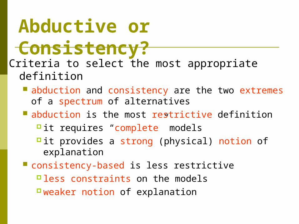
Criteria to select the most appropriate definition abduction and consistency are the two extremes of
a spectrum of alternatives abduction is the most restrictive definition
it requires “complete” models it provides a strong (physical) notion of
explanation consistency-based is less restrictive
less constraints on the models weaker notion of explanation
Abductive or Consistency?
oil_cup
normal holed
oil_level
normal low
oil_loss
oil_below_car
oil_gauge
normal red
radiatornormal holed
water_levelnormal low
water_tempnormal high
engine_tempnormal high
engine_on
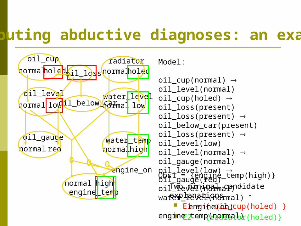
Computing abductive diagnoses: an example
Obs1 = {engine_temp(high)}Two minimal candidate explanations E1 = { oil_cup(holed) } E2 = {radiator(holed)}
Model:
oil_cup(normal) oil_level(normal)oil_cup(holed) oil_loss(present)oil_loss(present) oil_below_car(present)oil_loss(present) oil_level(low)oil_level(normal) oil_gauge(normal)oil_level(low) oil_gauge(red)oil_level(normal) water_level(normal)
engine(on) engine_temp(normal)...
Outline Last lecture:
1. Generation of tests/probes
2. Measurement Selection
3. Probabilities of Diagnoses
Today’s lecture:
1. Models of correct + faulty behavior
2. Sherlock engine
3. Abductive diagnosis
4. Qualitative models
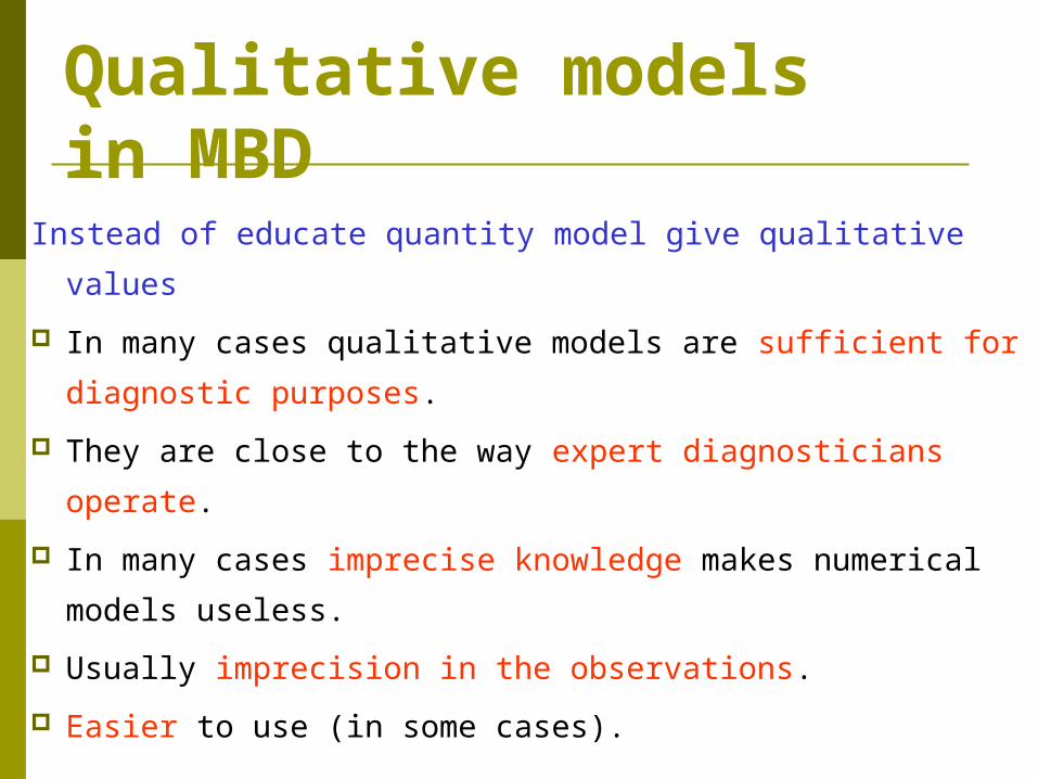
Qualitative models in MBD
Instead of educate quantity model give qualitative values
In many cases qualitative models are sufficient for
diagnostic purposes.
They are close to the way expert diagnosticians
operate.
In many cases imprecise knowledge makes numerical
models useless.
Usually imprecision in the observations.
Easier to use (in some cases).
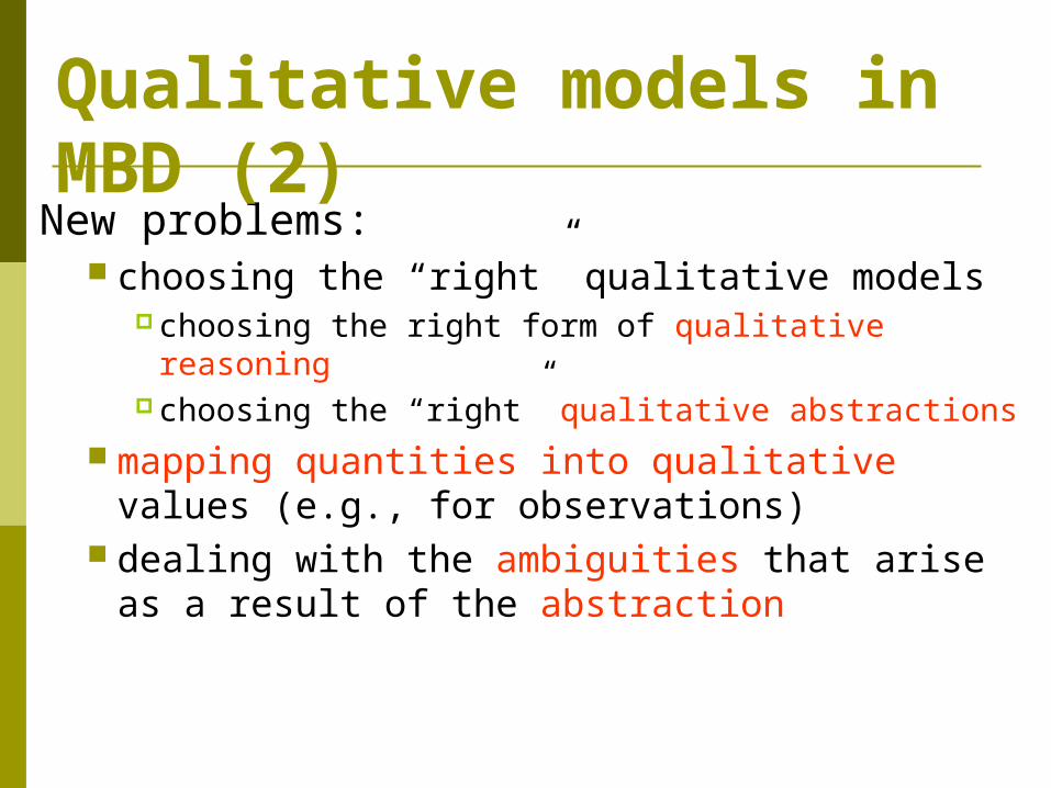
New problems: choosing the “right” qualitative models
choosing the right form of qualitative reasoning choosing the “right” qualitative abstractions
mapping quantities into qualitative values (e.g., for observations)
dealing with the ambiguities that arise as a result of the abstraction
Qualitative models in MBD (2)
A simple example
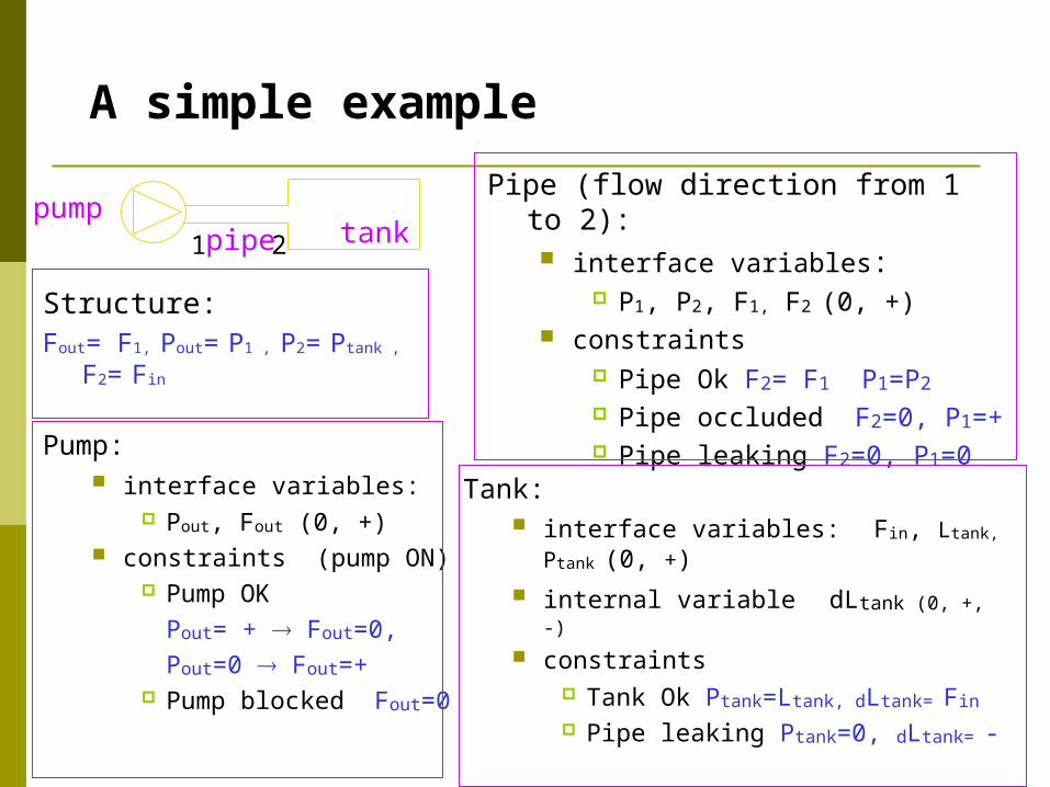
Pump: interface variables:
Pout, Fout (0, +) constraints (pump ON)
Pump OK Pout= + Fout=0, Pout=0 Fout=+ Pump blocked Fout=0
pipe tankpump
Pipe (flow direction from 1 to 2): interface variables:
P1, P2, F1, F2 (0, +) constraints
Pipe Ok F2= F1 P1=P2
Pipe occluded F2=0, P1=+ Pipe leaking F2=0, P1=0
Tank: interface variables: Fin, Ltank, Ptank
(0, +) internal variable dLtank (0, +, -)
constraints Tank Ok Ptank=Ltank, dLtank= Fin
Pipe leaking Ptank=0, dLtank= -
1 2
Structure:Fout= F1, Pout= P1 , P2= Ptank ,
F2= Fin
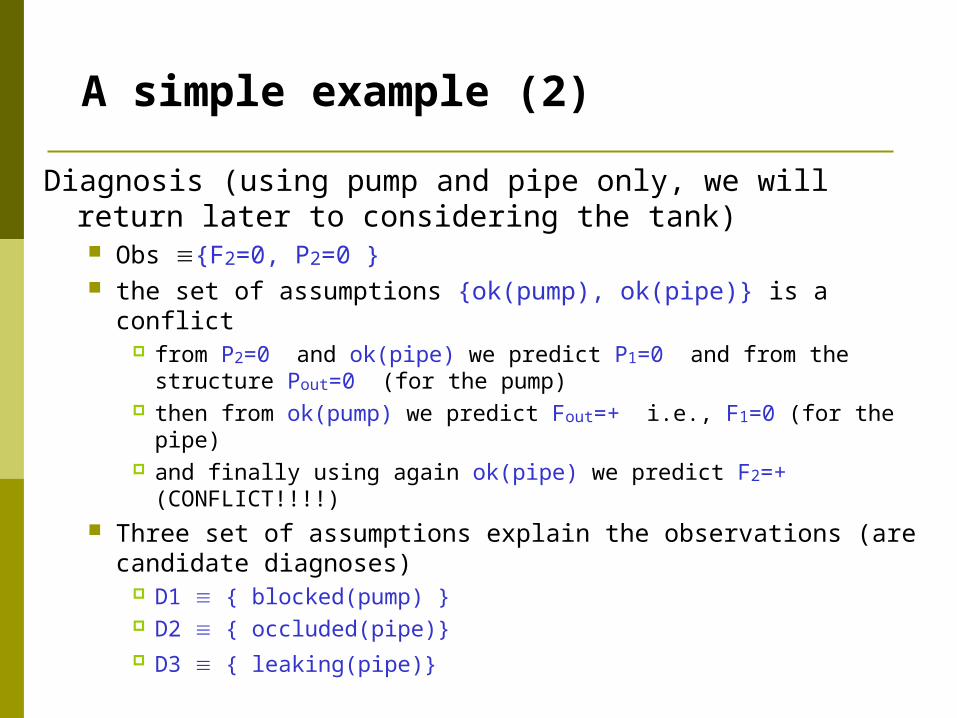
Diagnosis (using pump and pipe only, we will return later to considering the tank) Obs {F2=0, P2=0 } the set of assumptions {ok(pump), ok(pipe)} is a conflict
from P2=0 and ok(pipe) we predict P1=0 and from the structure Pout=0 (for the pump)
then from ok(pump) we predict Fout=+ i.e., F1=0 (for the pipe) and finally using again ok(pipe) we predict F2=+ (CONFLICT!!!!)
Three set of assumptions explain the observations (are candidate diagnoses)
D1 { blocked(pump) } D2 { occluded(pipe)} D3 { leaking(pipe)}
A simple example (2)
A second example
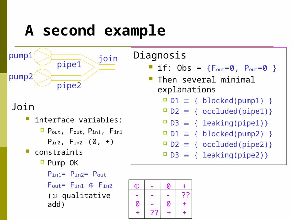
Join interface variables:
Pout, Fout, Pin1, Fin1
Pin2, Fin2 (0, +) constraints
Pump OK Pin1= Pin2= Pout
Fout= Fin1 Fin2
( qualitative add)
pipe1pump1
pipe2pump2
join Diagnosis if: Obs = {Fout=0, Pout=0 } Then several minimal
explanations D1 { blocked(pump1) } D2 { occluded(pipe1)} D3 { leaking(pipe1)} D1 { blocked(pump2) } D2 { occluded(pipe2)} D3 { leaking(pipe2)}
- 0 +- - - ??0 - 0 ++ ?? + +