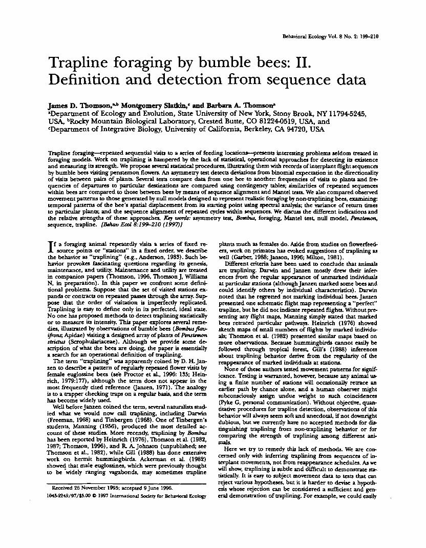
Behavioral Ecology Vol. 8 No. 2: 199-210

Trapline foraging by bumble bees: II.Definition and detection from sequence dataJames D. Thomson,*** Montgomery Slatirin,c and Barbara A. Thomson*•Department of Ecology and Evolution, State University of New York, Stony Brook, NY 11794-5245,USA, bRocky Mountain Biological Laboratory, Crested Butte, CO 81224-0519, USA, anddepartment of Integrative Biology, University of California, Berkeley, CA 94720, USA

Trapline foraging—repealed sequential visits to a series of feeding locations—presents interesting problems seldom treated inforaging models. Work on traplining is hampered by the lack of statistical, operational approaches for detecting its existenceand measuring its strength. We propose several statistical procedures, illustrating them with records of interplant flight sequencesby bumble bees visiting penstemon flowers. An asymmetry test detects deviations from binomial expectation in the directionalityof visits between pairs of plants. Several tests compare data from one bee to another frequencies of visits to plants and fre-quencies of departures to particular destinations are compared using contingency tables; similarities of repeated sequenceswithin bees are compared to those between bees by means of sequence alignment and Mantel tests. We also compared observedmovement patterns to those generated by null models designed to represent realistic foraging by non-traplining bees, examining:temporal patterns of the bee's spatial displacement from its starting point using spectral analysis; the variance of return timesto particular plants; and the sequence alignment of repeated cycles within sequences. We discuss the different indications andthe relative strengths of these approaches. Krj words: asymmetry test, Bombus, foraging, Mantel test, null model, Ptnsttwum,sequence, trapline. [Bthav Ecol 8:199-210 (1997)]

If a foraging animal repeatedly visits a series of fixed re-source points or "stations" in a fixed order, we describe

the behavior as "traplining" (e.g., Anderson, 1983). Such be-havior provokes fascinating questions regarding its genesis,maintenance, and utility. Maintenance and utility are treatedin companion papers (Thomson, 1996, Thomson J, WilliamsN, in preparation). In this paper we confront some defini-tional problems. Suppose that the set of visited stations ex-pands or contracts on repeated passes through the array. Sup-pose that the order of visitation is imperfectly replicated.Traplining is easy to define only in its perfected, ideal state.No one has proposed methods to detect traplining statisticallyor to measure its intensity. This paper explores several reme-dies, illustrated by observations of bumble bees (Bombus flav-ifrons, Apidae) visiting a designed array of plants of PtnsUwumstrictus (Scrophulariaceae). Although we provide some de-scription of what the bees are doing, the paper is essentiallya search for an operational definition of traplining.

The term "traplining" was apparently coined by D. H. Jan-zen to describe a pattern of regularly repeated flower visits byfemale cuglossine bees (see Proctor et aL, 1996: 135; Hein-rich, 1979:177), although the term does not appear in themost frequently cited reference (Janzen, 1971). The analogyis to a trapper checking traps on a regular basis, and the termhas become widely used.

Well before Janzen coined the term, several naturalists stud-ied what we would now call traplining, including Darwin(Freeman, 1968) and Tinbergen (1968). One of Tinbergen'sstudents, Manning (1956), produced the most detailed ac-count of these studies. More recently, traplining by Bombushas been reported by Heinrich (1976), Thomson et aL (1982,1987; Thomson, 1996), and R. A. Johnson (unpublished; seeThomson et aL, 1982), while GUI (1988) has done extensivework on hermit hummingbirds. Ackerman et aL (1982)showed that male euglossines, which were previously thoughtto be widely ranging vagabonds, may sometimes trapline

Received 26 November 1995; accepted 9 June 1996.1045-2249/97/15.00 O 1997 International Sodety for Behavioral Ecology

plants much as females do. Aside from studies on flowerfeed-ers, work on primates has evoked suggestions of traplining aswell (Garber, 1988;Janson, 1996; Milton, 1981).

Different criteria have been used to conclude that animal*are traplining. Darwin and Janzen mostly drew their infer-ences from die regular appearance of unmarked individualsat particular stations (although Janzen marked some bees andcould identify others by individual characteristics). Darwinnoted that he regretted not marking individual bees. Janzenpresented one schematic flight map representing a "perfect"trapline, but he did not indicate repeated flights. Without pre-senting any flight maps. Manning simply stated that markedbees retraced particular pathways. Heinrich (1976) showedsketch maps of small numbers of flights by marked individu-als; Thomson et aL (1982) presented similar maps based onmore observations. Because hummingbirds cannot easily befollowed through tropical forest. Gill's (1988) inferencesabout traplining behavior derive from the regularity of diereappearance of marked individuals at stations.

None of these authors tested movement patterns for signif-icance. Testing is warranted, however, because any animal us-ing a finite number of stations win occasionally retrace anearlier path by chance alone, and a human observer mightsubconsciously assign undue weight to such coincidences(Pyke G, personal communication). Without objective, quan-titative procedures for trapline detection, observations of diisbehavior will always seem soft and anecdotal, if not downrightdubious, but we currently have no accepted methods for dis-tinguishing traplining from non-traplining behavior or forcomparing the strength of traplining among different ani-mals.

Here we try to remedy this lack of methods. We are con-cerned only with inferring traplining from sequence* of in-terplant movements, not from reappearance schedules. As wewill show, traplining is subtle and difficult to demonstrate sta-tistically. It is easy to subject movement data to tests that canreject various hypotheses, but it is harder to devise a hypoth-esis whose rejection can be considered a sufficient and gen-eral demonstration of traplining. For example, we could easily

200 Behavioral Ecology VoL 8 No. 2

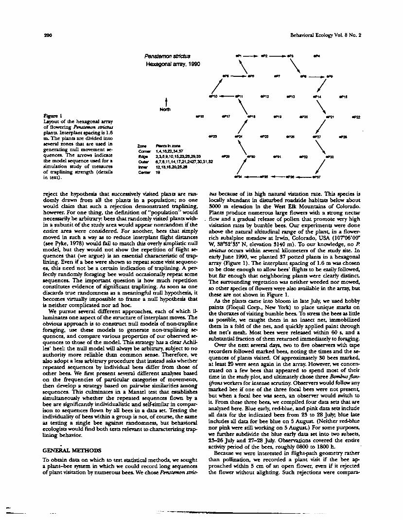
Figure 1Layout of the hexagonal arrayof flowering PmsUmon strictuiplants. Interplant roaring is 1.6m. The plants are divided intoseveral zones that are used ingenerating null movement se-quences. The arrows indicatethe model sequence used for asimulation study of measuresof traplining strength (detailsin text).

Penstemon strictua

Hexagonal array, 1990

North

mn • «P2 » «PI

\ \

«PK> - »

•P23

Zone Plsnts In zoneComar 1,4,18^2,34.37

Outer 8,7,8.11.14,17.21,2427,30,31.32Irawr 12.13,18,2025.28Cwter 10

m

•P24

\

«P13

«P20

•P2S «P27

\

reject the hypothesis that successively visited plants are ran-domly drawn from all the plants in a population; no onewould claim that such a rejection demonstrated traplining,however. For one thing, the definition of "population" wouldnecessarily be arbitrary: bees that randomly visited plants with-in a subunit of the study area would appear nonrandom if theentire area were considered. For another, bees that simplymoved in such a way as to reduce interplant flight distances(see Pykc, 1978) would fail to match this overly simplistic nullmodel, but they would not show the repetition of flight se-quences that (we argue) is an essential characteristic of trap-lining. Even if a bee were shown to repeat some visit sequenc-es, this need not be a certain indication of traplining. A per-fectly randomly foraging bee would occasionally repeat somesequences. The important question is how much repetitionconstitutes evidence of significant traplining. As soon as onediscards true randomness as a meaningful null hypothesis, itbecomes virtually impossible to frame a null hypothesis thatis neither complicated nor ad hoc.

We pursue several different approaches, each of which il-luminates one aspect of the structure of interplant moves. Theobvious approach is to construct null models of non-traplineforaging, use these models to generate non-traplining se-quences, and compare various properties of our observed se-quences to those of the model. This strategy hat a clear Achil-les' heel: the null model will always be arbitrary, subject to noauthority more reliable than common sense. Therefore, wealso adopt a less arbitrary procedure that instead asks whetherrepeated sequences by individual bees differ from those ofother bees. We first present several different analyses basedon the frequencies of particular categories of movements,then develop a strategy based on pairwise similarities amongsequences. This culminates in a Mantel test that establishessimultaneously whether the repeated sequences flown by abee are significantly individualistic and self-cnnilar in compar-ison to sequences flown by all bees in a data set. Testing theindividuality of bees within a group is not, of course, the sameas testing a single bee against randomness, but behavioralecologists would find both tests relevant to characterizing trap-lining behavior.

GENERAL METHODS

To obtain data on which to test statistical methods, we soughta plant-bee system in which we could record long sequencesof plant visitation by numerous bees. We chose PensUmon stric-

tus because of its high natural vistation rate. This specie* islocally abundant in disturbed roadside habitats below about3000 m elevation in the West Elk Mountains of Colorado.Plants produce numerous large flowers with a strong nectar

. flow and a gradual release of pollen that promote very highvisitation rates by bumble bees. Our experiments were doneabove the natural altitudinal range of the plant, in a flower-rich subalpine meadow at Irwin, Colorado, USA (107°06'00"W, 38°52'35' N, elevation 3140 m). To our knowledge, no P.strictus occurs within several kilometers of the study site. Inearly June 1990, we planted 37 potted plants in a hexagonalarray (Figure 1). The interplant spacing of 1.6 m was chosento be close enough to allow bees' flights to be easily followed,but far enough that neighboring plants were clearly distinctThe surrounding vegetation was neither weeded nor mowed,so other species of flowers were also available in the array, butthese are not shown in Figure 1.

As the plants came into bloom in late July, we used hobbypaints (Floquil Corp., New York) to place unique marks onthe thoraxes of visiting bumble bees. To stress the bees as littleas possible, we caught them in an insect net, immobilizedthem in a fold of the net, and quickly applied paint throughthe net's mesh. Most bees were released within 60 s, and asubstantial fraction of them returned immediately to foraging.

Over the next several days, two to five observers with taperecorders followed marked bees, noting the times and the se-quences of plants visited. Of approximately 30 bees marked,at least 20 were seen again in the array. However, we concen-trated on a few bees that appeared to spend most of theirtime in the study plot, and ultimately chose three Bombusflav-ifrons workers for intense scrutiny. Observers would follow anymarked bee if one of the three focal bees were not present,but when a focal bee was seen, an observer would switch toit. From these three bees, we compiled four data sets that areanalyzed here. Blue early, red-blue, and pink data sets includeall data for the indicated bees from 23 to 28 Jury; blue lateinclude* all data for bee blue on 5 August (Neither red-bluenor pink were still working on 5 August) For some purposes,we further subdivide the blue early data set into two subsets,23-26 July and 27-28 July. Observations covered the entireactivity period of the bees, roughly 0800 to 1800 h.

Because we were interested in flight-path geometry ratherthan pollination, we recorded a plant visit if the bee ap-proached within 5 cm of an open flower, even if it rejectedthe flower without alighting. Such rejections were compare-

Thomson et sd. * Traplining by bees 201

lively rare; more often, the bee landed for at least a briefinspection before rejecting a plant

Even with dose observation, we occasionally lost sight of abee in mid-sequence. Unless it was sighted again within a fews, we terminated the sequence, beginning a new sequencewhen the bee was rediscovered. All the bees occasionally vis-ited flowers other than Ptnsttmon stridus. Such visits were re-corded on tape, and the locations of the non-PtnsUwum plantswere mapped, but the analyses presented here exclude non-Pttutemon visits. Thus a sequence of Ptnsttmon 3 to HtUniumto Ptnsttmon 5 is here recorded as Ptnsttmon 3 to PtnsUmon5. Almost all the non-Ptnstrmon visits were short breaks inwhat was overwhelmingly itoutemon-dominated foraging; how-ever, pink was an exception, in that she began to regularlyinclude several Lupinus sp. plants in her foraging, especiallyon 27-28 July.

The various statistical treatments of the data are describedseparately below. Where our purpose is primarily to illustratea methodology, we may show the analysis only for selecteddata sets.

RESULTS

Foraging time budget!

The three focal bees spent most of their foraging time in thearray. This was best documented for blue on 5 August. A sin-gle observer tried to follow this bee (and no others) contin-uously from about 0900 until about 1530 h, taking brief breakswhen the bee appeared to be leaving for the hive. The totalobservation period, including breaks, was 22,485 s; blue wasin sight for 20,482 s, or 91.1% of the total As the observernever saw the bee enter the array, but found her only aftershe had begun foraging, the 91.1% figure underestimates thetime she truly spent in the array. We infer that she probablyforaged entirely within the array, spending the remaining 5%or so of her time flying to and from the nest and depositingor picking up food there.

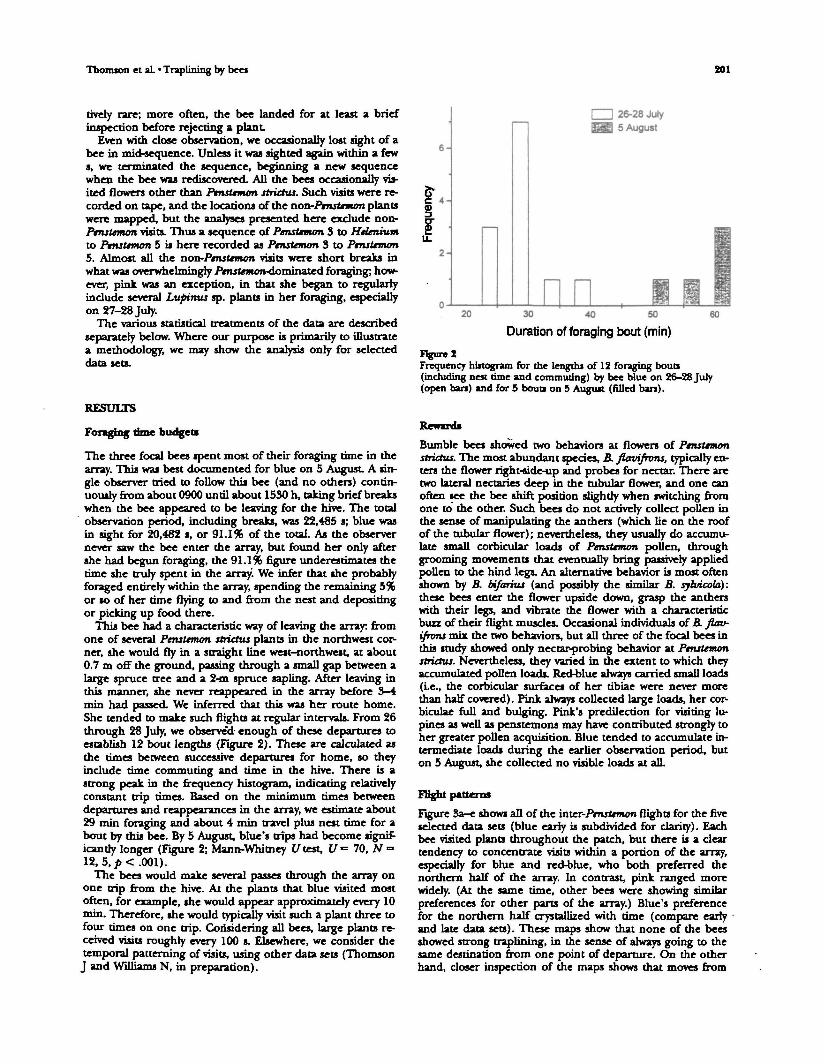
This bee had a characteristic way of leaving the array: fromone of several Pmstemon stridus plants in the northwest cor-ner, she would fry in a straight line west-northwest, at about0.7 m off the ground, passing through a small gap between alarge spruce tree and a 2-m spruce sapling. After leaving inthis manner, she never reappeared in the array before 3-4min had passed. We inferred that this was her route home.She tended to make such flights at regular intervals. From 26through 28 Jury, we observed- enough of these departures toestablish 12 bout lengths (Figure 2). These are calculated asthe times between successive departures for home, so theyinclude time commuting and time in the hive. There is astrong peak in the frequency histogram, indicating relativelyconstant trip times. Based on the minimum times betweendepartures and reappearances in the array, we estimate about29 min foraging and about 4 min travel plus nest time for about by this bee. By 5 August, blue's trips had become signif-icantly longer (Figure 2; Mann-Whitney I/test, [/«= 70, N =12, 5, p < .001).

The bees would make several passes through the array onone trip from the hive. At the plants that blue visited mostoften, for example, she would appear approximately every 10min. Therefore, she would typically visit such a plant three tofour times on one trip. Considering all bees, large plants re-ceived visits roughly every 100 s. Elsewhere, we consider thetemporal patterning of visits, using other data sets (ThomsonJ and Williams N, in preparation).

6 -

2 -

I I 26-28 July5 August

nn20 30 60

Duration of foraging bout (min)

Figure tFrequency histogram for the lengths of 12 foraging bouts(including nest time and commuting) by bee blue on 26-28 July(open ban) and for 5 bouts on 5 August (filled bars).

Rewards

Bumble bees showed two behaviors at flowers of PtnsUmonstridus. The most abundant species, B. flavifwns, typically en-ters the flower right-side-up and probes for nectar. There aretwo lateral nectaries deep in the tubular flower, and one canoften see the bee shift position slightly when switching fromone to the other. Such bees do not actively collect pollen inthe sense of manipulating the anthers (which lie on the roofof the tubular flower); nevertheless, they usually do accumu-late small corbicular loads of PtnsUmon pollen, throughgrooming movements that eventually bring passively appliedpollen to the hind legs. An alternative behavior is most oftenshown by B. bifarius (and possibly the «imilar B. syhncola):these bees enter the flower upside down, grasp the antherswith their legs, and vibrate the flower with a characteristicbuzz of their flight muscles. Occasional individuals of B flao-ifrons mix the two behaviors, but all three of the focal bees inthis study showed only nectar-probing behavior at Pmstemonstridus. Nevertheless, they varied in the extent to which theyaccumulated pollen loads. Red-blue always carried small loads(Le., the corbicular surfaces of her tibiae were never morethan half covered). Pink always collected large loads, her cor-biculae full and bulging. Pink's predilection for visiting lu-pines as well as penstemons may have contributed strongly toher greater pollen acquisition. Blue tended to accumulate in-termediate loads during the earlier observation period, buton 5 August, she collected no visible loads at all.

Flight patterns

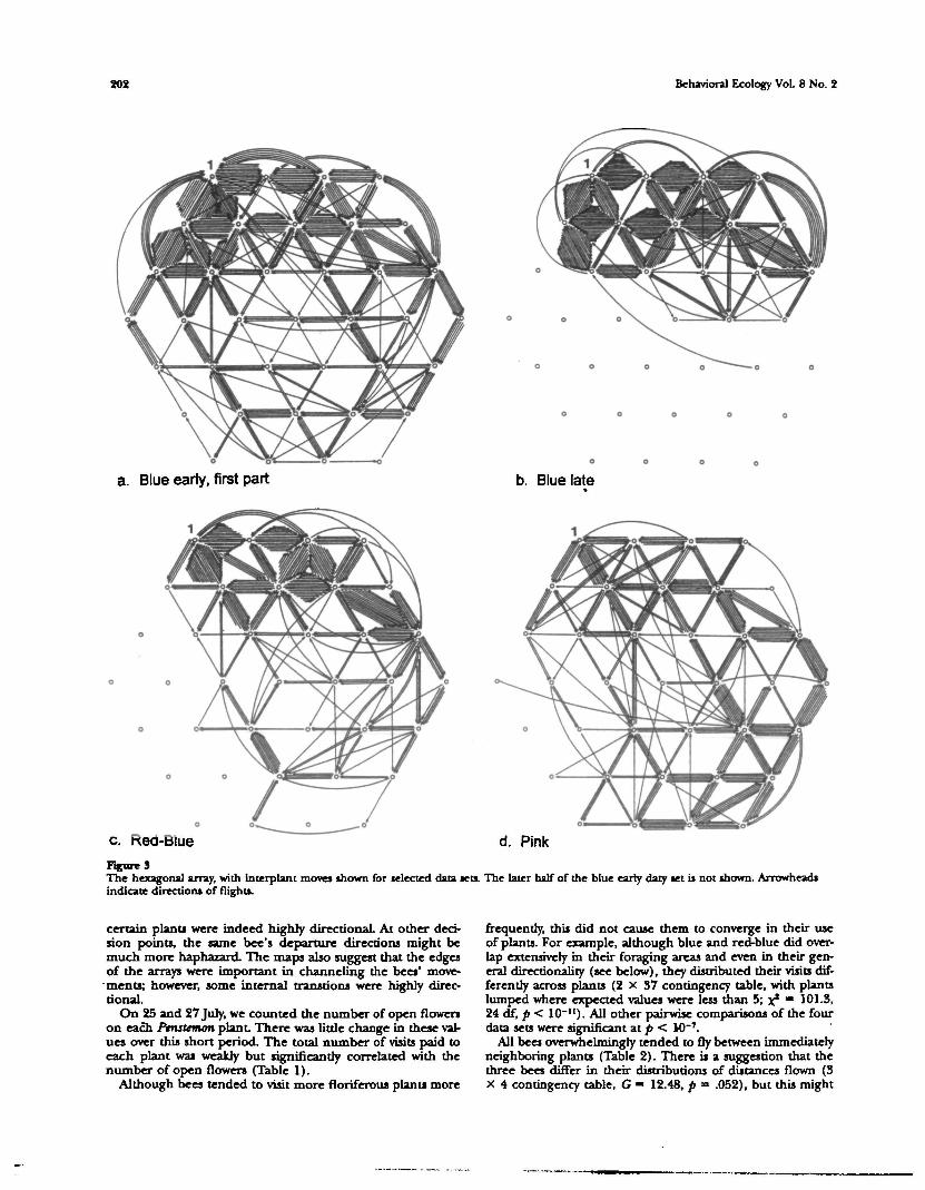
Figure 3a-e shows all of the intcx-Ptnsttmon flights for the fiveselected data sets (blue early is subdivided for clarity). Eachbee visited plants throughout the patch, but there is a cleartendency to concentrate visits within a portion of the array,especially for blue and red-blue, who both preferred thenorthern half of the array. In contrast, pink ranged morewidely. (At the same time, other bees were showing similarpreferences for other parts of the array.) Blue's preferencefor the northern half crystallized with time (compare early 'and late data sets). These maps show that none of the beesshowed strong traplining, in the sense of always going to thesame destination from one point of departure. On the otherhand, closer inspection of the maps shows that moves from

202 Behavioral Ecology VoL 8 No. 2

a. Blue earty, first part

o o e o o

o o o

b. Blue late

c Rea-biue d. Pink

Figure SThe hexagonal array, with interplant moves shown for selected data sets. The later half of the blue early daty set is not shown. Arrowheadsindicate directions of flights.

certain plants were indeed highly directional. At other deci-sion points, the same bee's departure directions might bemuch more haphazard. The maps also suggest that the edgesof the arrays were important in channeling the bees' move-ments; however, some internal transtions were highly direc-tional

On 25 and 27 July, we counted the number of open flowerson each Ptnstemon plant. There was little change in these val-ues over this short period. The total number of visits paid toeach plant was weakly but significantly correlated with thenumber of open flowers (Table 1).

Although bees tended to visit more floriferous plants more

frequently, this did not cause them to converge in their useof plants. For example, although blue and red-blue did over-lap extensively in their foraging areas and even in their gen-eral directionality (see below), they distributed their visits dif-ferently across plants (2 X 37 contingency table, with plantslumped where expected values were less than 5; x* m 101.3,24 df, p < 10""). All other pairwise comparisons of the fourdata sets were significant at p < W'1.

All bea overwhelmingly tended to fly between immediatelyneighboring plants (Table 2). There is a suggestion that thethree bees differ in their distributions of distances flown (3X 4 contingency table, G - 12.48, p ™ .052), but this might

Thomson et aL • Traplining by bed 203

Table 1Pearson correlnumber of flowers open on that plant for Tarioot data Kts (H « 37for each)

i of the number of visits to a plant and dieTabletClassification of in

Flower census

Data set 25 July 27 July

Blue, 23-26 JulyBlue, 27-28 JulyRed-blue, 23-28 JulyPink, 23-28 July

0.452**0.474**0.504 (m)0.505**

0.502**0322**0.351*0.524**

.05; .01.

reflect differences in opportunity rather than differences inflight behavior bees that foraged more often at the edges ofthe array, as opposed to the center, faced a somewhat differentdistribution of potential neighbor categories.

Tramllion matrices and an i metry teatThe next series of tests are based on the transition matrix,where each interplant movement is cast into a 37 X 37 table.Rows indicate the plant the bee moved from, columns indi-cate the plant a bee moved to. If a traplining bee follows aparticular path each time it passes through an array of plants,we would expect the transition matrix to be asymmetricalabout the main diagonal; for example, the number of movesfrom plant 1 to 2 would differ from the number from 2 to 1.Our test followed a suggestion of Oden's, previously used bySokal (1991): for each pair of plants, we calculated the bino-mial probability of the observed departure from a 1:1 expec-tation. To test the entire transition matrix, we used Fisher'smethod of combining probabilities (Sokal and Rohlf, 1995:794). We eliminated from consideration any plant pairs forwhich the data set contained fewer than six transitions, be-cause such pairs give little information on directionality andtherefore dilute the test's effectiveness. By this procedure, alldata sets for blue and red-blue showed highly significant asym-metry (J> < .01), but pink's movements did not (p > .05).Further trimming the data set to eliminate pairs with <10transitions did not change these results. Note that this tech-nique detects only unidirectional traplining: if a bee com-muted back and forth along a particular sequence of plants,transitions would be symmetrical, even though we would con-sider such commuting to constitute a special case of traplin-ing.

IVapfine skeleton *W*ywm

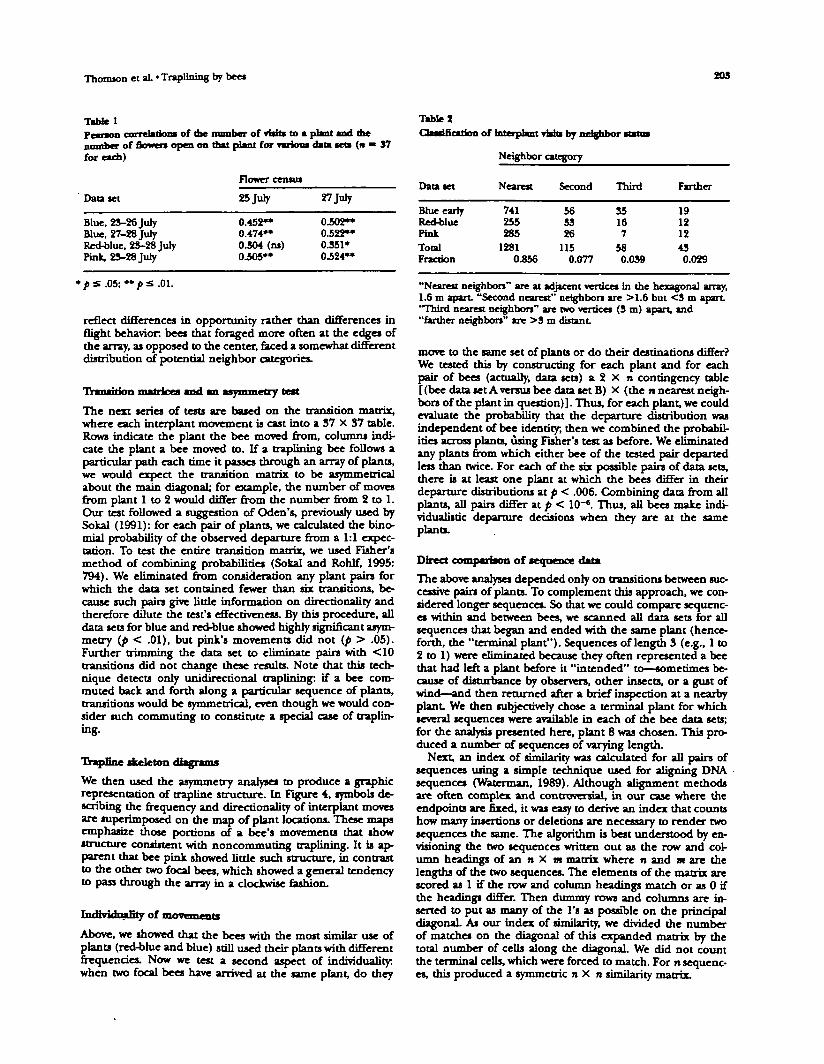
We then used the asymmetry analyses to produce a graphicrepresentation of trapline structure. In Figure 4, symbols de-scribing the frequency and directionality of interplant movesare superimposed on the map of plant locations. These mapsemphasize those portions of a bee's movements that showstructure consistent with noncommuting traplining. It is ap-parent that bee pink showed little such structure, in contrastto the other two focal bees, which showed a general tendencyto pass through the array in a clockwise fashion.

Individuality of movements

Above, we showed that the bees with the most nimilar use ofplants (red-blue and blue) still used their plants with differentfrequencies. Now we test a second aspect of individuality,when two focal bees have arrived at the same plant, do they

Tptant viste by neighbor statin

Neighbor category

Data set Nearest Second Third Farther

Blue earlyRed-bluePinkToolFraction

741255285

12810.856

563326

1150.077

35167

580.039

191212430.029

"Nearest neighbors" are at adjacent vertices in the hexagonal array,1.6 m apart. "Second nearest" neighbors are >1.6 but <3 m apart."Third nearest neighbors" are two vertices (3 m) apart, and"farther neighbors" are >3 m distant.

move to the same set of plants or do their destinations differ?We tested this by constructing for each plant and for eachpair of bees (actually, data sets) a 2 X n contingency table[(bee data set A versus bee data set B) X (the n nearest neigh-bors of the plant in question) ] . Thus, for each plant, we couldevaluate the probability that the departure distribution wasindependent of bee identity; then we combined the probabil-ities across plants, using Fisher's test as before. We eliminatedany plants from which either bee of the tested pair departedless than twice. For each of the six possible pairs of data sets,there is at least one plant at which the bees differ in theirdeparture distributions at p < .006. Combining data from allplants, all pairs differ at p < 10~*. Thus, all bees make indi-vidualistic departure decisions when they are at the sameplants.

Direct comparison of sequence data

The above analyses depended only on transitions between suc-cessive pain of plants. To complement this approach, we con-sidered longer sequences. So that we could compare sequenc-es within and between bees, we scanned all data sets for allsequences that began and ended with the same plant (hence-forth, the "terminal plant"). Sequences of length 3 (e.g., I to2 to 1) were eliminated because they often represented a beethat had left a plant before it "intended" to—sometimes be-cause of disturbance by observers, other insects, or a gust ofwind!—and then returned after a brief inspection at a nearbyplant We then subjectively chose a terminal plant for whichseveral sequences were available in each of the bee data sets;for the analysis presented here, plant 8 was chosen. This pro-duced a number of sequences of varying length.

Next, an index of similarity was calculated for all pairs ofsequences using a simple technique used for aligning DNA -sequences (Waterman, 1989). Although alignment methodsare often complex and controversial, in our case where theendpoints are fixed, it was easy to derive an index that countshow many insertions or deletions are necessary to render twosequences the same. The algorithm is best understood by en-visioning the two sequences written out as the row and col-umn headings of an n X m matrix where n and m are thelengths of the two sequences. The elements of the matrix arescored as 1 if the row and column headings m^trh or as 0 ifthe headings differ. Then dummy rows and columns are in-serted to put as many of the l's as possible on the principaldiagonaL As our index of similarity, we divided the numberof matches on the diagonal of this expanded matrix by thetotal number of cells along the diagonaL We did not countthe terminal cells, which were forced to match. For n sequenc-es, this produced a symmetric nX n similarity matrix.

204 Behavioral Ecology VoL 8 No. 2

• • o •

a Blue early, first part

b. Blue late

Figure 4TrapUne skeleton maps summarizing the raw maps shown in Figure S. Arrows indicate Interplant transitions for which the bee in questionshowed directionality. The size of the arrowhead indicates the significance of the directionality: large, medium, and small arrowheads denotep levels of .01, .05, and .1, respectively. The size of the shaft of die arrow indicates the total number of transitions observed: large, £15;medium, 9-14; small, 6-8. Where directionality was Insignificant even though traffic was high (p > .1), diamonds denote sample size (largediamonds, 215 transitions; small diamonds, 6-14). Stars indicate non-Ptnsttmon plants (not included in numerical analyses). No map isshown for the pink data set because so few transitions showed significant directionality.

The similarity matrix could be subjected to any of the stan-dard ordination or clustering techniques that employ suchma trices. Because we were more interested in a significancetest for traplining, we m t̂i-a^ used a Mantel test (Mantel,1967; Sokal, 1979; Sokal and Rohlf, 1995). as follows. We pro-duced an n X n design matrix that contained 1 's in the cellswhere the similarity matrix contained sequences produced bythe same bee and 0's in the cells where the similarity matrixcontained sequences produced by different bees. That is, thedesign matrix represents an ideal case in which all sequencesgenerated by one bee show perfect similarity, and all sequenc-es generated by different bees are completely different TheMantel procedure computes a correladonlike statistic r (thestandardized Mantel statistic), that shows how closely the ob-served similarity matrix resembles the ideal design matrix. Toassess the significance of r, a randomization process then per-mutes the values in the similarity matrix by redistributing thevalues across the rows and columns. We produced 999 per-mutations, calculating rfor each one and comparing the trueobserved value of r to the distribution of the 999 randomizedversions. The observed matrix was more similar to the designmatrix (r = .162) than any of the 999 randomizations, i.e., p< .001. Therefore, sequences within bees (or, more precisely,within data sets, because the bhie early and blue late sets arehere being contrasted as if they were from different bees)

resemble each other significantly more closely than they re-semble sequences from different bees.

Generating null sequences

Rather than comparing bees with each other, we now compareeach data set to neutral expectations. As noted in the intro-duction, the simplest hypotheses for non-traplining move-ment (e.g., random plant choices) are too simplistic to beinformative about traplining. We know that bees tend to movetoward near neighbors in many circumstances (Morse, 1982),including our array (Table 2). Our data would emphaticallyreject the hypothesis of random moves, but we would not con-sider this to demonstrate traplining. Tnstrad, we take the ob-served tendency to make short moves as a fundamental com-ponent of foraging that we would expect to see in non-trap-lining and traplining bees alike. It forms a basic constraint inour nuD model. As an additional constraint, we also regard abee's aversion to returning to just-visited plants as anotherfundamental component For a bee to be traplining, in thisview, its movements must contain a higher-order repetitivestructure that cannot be produced by the simple action ofthese two constraints.

We could not simply use the observed probabilities of first,second, etc., nearest-neighbor moves to condition the null

Thomson et aL • Traplining by bees 205

Blue early, longest sequence in data set

10 20 30 40 50 60

Step number (for displacement); Frequency dass (for penodogram bars)

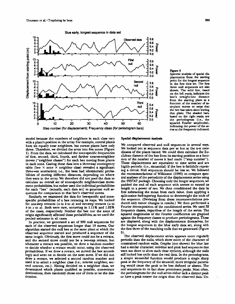
Figure 5Spectral analyst of spatial dis-placements from the starlingpoint for the longest sequencein the tint data set. The ftrstthree null sequences are alsoshown. The solid line, basedon the left y-axis, indicates thebee's straight-line distancefrom the starting plant as afunction of the number of in-terplant moves or steps thatthe bee has taken since leavingthat plant. The shaded bars,based on the right y-axis, arethe penodogram (i.e., thesquared Fourier amplitudes),indicating the power of the se-ries at the frequency indicated.

model because the numbers of neighbors in each dass varywith a plant's position in the array. For example, central plantshave six equally near neighbors, but corner plants have onlythree. Therefore, we divided the array into five zones (Figure1). From the data, we calculated the zone-specific frequenciesof first, second, third, fourth, and farther nearest-neighbormoves ("neighbor classes") for each bee moving from plantsin each zone. Casting these data into a three-way contingencytable (bee X zone X neighbor class) revealed a significantthree-way interaction; i.e., the bees had idiosyncratic proba-bilities of moving different distances, depending on wherethey were in the array. We therefore did not pool the data tocalculate an overall set of zone-specific neighbor-class move-ment probabilities, but rather used the individual probabilitiesfor each "bee" (actually, each data set) to generate null se-quences for comparison to that bee's observed moves.

Similarly, we examined the data for bee-specific and zone-specific probabilities of a bee retracing its steps. We lookedfor one-step retraces (a to b to a) and two-step retraces (a to* to c to a). Both were rare, occurring in 1.11% and 1.92%of the cases, respectively. Neither the bee nor the zone oforigin significantly affected these probabilities, so we used thepooled estimates in all cases.

In practice, we generated a set of 999 null sequences foreach of the observed sequences longer than 19 moves. Ouralgorithm started the null bee at the same plant at which theobserved sequence started and produced a sequence of thesame length. Obviously, the first move could not be a retrace,and the second move could not be a two-step retrace, butwhenever a retrace was possible, we drew a random numberto dedde whether a retrace would occur, using the observedprobabilities. If we drew a retrace, we moved the bee accord-ingly and went on to dedde on the next move. If we did notdraw a retrace, we selected a second random number andused it'to select a neighbor class (i.e., nearest neighbor, sec-ond nearest, etc.). Having dedded on a neighbor class, wedetermined which plants qualified as possible, non-retracedestinations, then randomly chose one of them to be the des-tination.

Spatial dfapla rtinalyn

We compared observed and null sequences in several ways.We looked not at sequence data per se but at the x-y coor-dinates of the plants visited. We could then calculate die Eu-clidean distance of the bee from its starting position as a func-tion of the number of moves it had made ("step number").These displacements are equivalent to time series and arehighly periodic (Le., sinusoidal) if the bee is faithfully repeat-ing a circuit. Null sequences should be less so. We followedthe recommendations of Wilkinson (1990) to compute spec-tral analyses of the periodicity of the displacement series usingthe SYSTAT package. Choosing only the longer sequences, wepadded the end of each sequence with zeroes to extend itslength to a power of two. We then conditioned the data byfirst subtracting the mean from each value, then applying asplit-cosine-bell-tapering function to downweight the ends ofthe sequence. (Deviating from these recommendations pro-duced only minor changes in results.) We then performed aFourier decomposition of the conditioned series. We used 32frequency classes, regardless of the length of the series. Thesquared magnitudes of the Fourier coefficients are graphedagainst the frequency classes to produce periodograms. Theseare displayed, along with the displacements themselves, forthe longest sequences in the blue early data set, along withthe first three of the matching nulls that we generated (Figure5).

The observed displacement series appears more regularlyperiodic than the nulls, which show more of the character ofconstrained random walks. Graphs (not shown) for blue latehad a similar character; red-blue and pink had sequences thatwere too short to show such dear cydidry, although the nullsstill looked less cyclic than the real data. In the periodograms,a simple sinusoidal function would produce a single sharppeak at the frequency of the sinusoid; more irregular pattern-'ing would cause the peak to be less defined or absent Thereal sequences do in fact show prominent peaks. Most often,the periodograms for the null series either lack a distinct peakor have a peak nearer the origin than the observed data. Un-

206 Behavioral Ecology VoL 8 No. 2

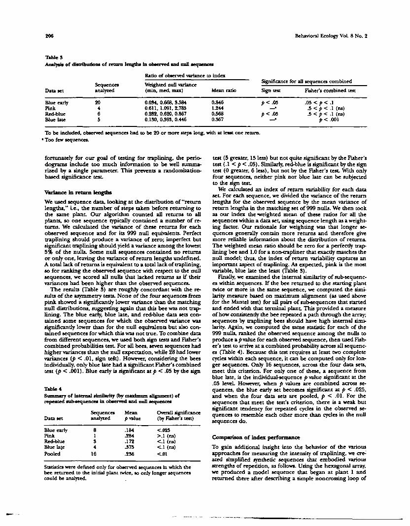
TableSAnalysis of distributions of return

Data setSequencesanalyzed

in observed and null sequences

Ratio of observed variance to index

Weighted null variance(inin, med, max) Mean ratio

Significance for all sequences combined

Sign test Fisher's combined test

Blue earlyPinkRed-blueBlue late

20465

0.034, 0.668. 3.5840.611, 1.091. 2,7850.282, 0.620, 0.8670.130, 0393, 0.446

0.8461.2440.5680.367

p< .03__•

p< .05—'

.05 < p < .1£ < p < .1 (ns)£ < p< .1 (ns)

p< .001

To be included, observed sequences had to be 20 or more steps long, with at least one return.•Too few sequences.

fortunately for our goal of testing for traplining, the perio-dograms include too much information to be well summa-rized by a single parameter. This prevents a randomization-based significance test.

^ r i m c c in return lengths

We used sequence data, looking at the distribution of "returnlengths," i.e., the number of steps taken before returning tothe same plant Our algorithm counted all returns to allplants, so one sequence typically contained a number of re-turns. We calculated the variance of these returns for eachobserved sequence and for its 999 null equivalents. Perfecttraplining should produce a variance of zero; imperfect butsignificant traplining should yield a variance among the lowest5% of the nulls. Some null sequences contained no returnsor only one, leaving the variance of return lengths undefined.A total lack of returns is equivalent to a total lack of traplining,so for ranking the observed sequence with respect to the nullsequences, we scored all nuLU that lacked returns as if theirvariances had been higher than the observed sequences.

The results (Table 3) are roughly concordant with the re-sults of the asymmetry tests. None of the four sequences frompink showed a significantly lower variance than the matchingnull distributions, suggesting again that this bee was not trap-lining. The blue early, blue late, and red-blue data sets con-tained some sequences for which the observed variance wassignificantly lower than for the null equivalents but also con-tained sequences for which this was not true. To combine datafrom different sequences, we used both sign tests and Fisher'scombined probabilities test. For all bees, seven sequences hadhigher variances than the null expectation, while 28 had lowervariances (p < .01, sign test). However, considering the beesindividually, only blue late had a «ignifir?nt Fisher's combinedtest (p < .001). Blue early is significant at p < .05 by the sign

T»ble 4

repeated sab-aequence* in observed and mill sequences

Data set

Blue earlyPinkRed-blueBlue lajePooled

Sequencesanalyzed

8134

16

Meanp value

.184

.284

.172J75.236

Overall significance(by Fisher's test)

<.O25>.l (ns)<-l (ns)<.l (ns)<.01

Statistics were denned only for observed sequences in which diebee returned to the initial plant twice, so only longer sequencescould be analyzed.

test (5 greater, 15 less) but not quite significant by the Fuher'stest (.1 < p < .05). Similarly, red-blue is significant by the signtest (0 greater, 6 less), but not by the Fisher's test. With onlyfour sequences, neither pink nor blue late can be subjectedto the sign test.

We calculated an index of return variability for each dataset. For each sequence, we divided the variance of the returnlengths for the observed sequence by the mean variance ofreturn lengths in the matching set of 999 nulls. We then tookas our index die weighted mean of these ratios for all thesequences within a data set, using sequence length as a weight-ing factor. Our rationale for weighting was that longer se-quences generally contain more returns and therefore givemore reliable information about the distribution of returns.The weighted mean ratio should be zero for a perfectly trap-lining bee and 1.0 for a non-trapliner that exactly matches thenull model; thus, the index of return variability captures animportant aspect of traplining. As expected, pink is the mostvariable, blue late the least (Table 3).

Finally, we examined die internal similarity of sub-sequenc-es within sequences. If the bee returned to the starting planttwice or more in die same sequence, we computed the simi-larity measure based on nmimnm alignment (as used abovefor the Mantel test) for all pairs of sub-sequences that startedand ended widi that terminal plant. This provided a measureof how consistently die bee repeated a path through the array;sequences by traplining bees should have high internal simi-larity. Again, we computed die same statistic for each of the999 nulls, ranked die observed sequence among die nulls toproduce a p value for each observed sequence, then used Fish-er's test to arrive at a combined probability across all sequenc-es (Table 4). Because this test requires at least two completecycles within each sequence, it can be computed only for lon-ger sequences. Only 16 sequences, across die four data sets,meet this criterion. For only one of these, a sequence fromblue late, is die individual-sequence p value significant at die.05 level However, when p values are combined across se-quences, die blue early set becomes significant at p < .025,and when die four data sets are pooled, p < .01. For diesequences that meet the test's criterion, mere is a weak butsignificant tendency for repeated cycles in die observed se-quences to resemble each other more than cycles in die nullsequences do.

Comparison of J**Am*r perfonnrace

To gain additional insight into die behavior of die variousapproaches for measuring die intensity of traplining, we cre-ated simplified synthetic sequences that embodied variousstrengths of repetition, as follows. Using die hexagonal array,we produced a model sequence diat began at plant 1 andreturned mere after describing a simple noncrossing loop of

Thomson et aL • Traplining by bees tO7

20 nearest-neighbor steps with no first-or second-step retrace*.We then simulated sequences of 401 steps in which "bees"started at plant 1, then repeated this path with varying de-grees of fidelity determined by a trapline-strength parameter,L When the bee was at any plant in the model sequence, itmoved to the next plant in the model sequence with proba-bility L With probability (1 - f), the bee moved randomly toany nearest neighbor. When the bee strayed from the modelsequence, it moved to randomly chosen nearest neighbors un-til it returned to a plant in the model sequence. Thus, for t» 1.0, the bee repeated the model path exactly, returning toplant 1 after 20 identical drcuits of perfect traptining. For t— 0, the bee moved in a random nearest-neighbor walk, sub-ject to the constraint on retraces: no traplining. For inter-mediate value* of t, the bee would tend to follow the modelpath but would be subject to getting lost more or less often.

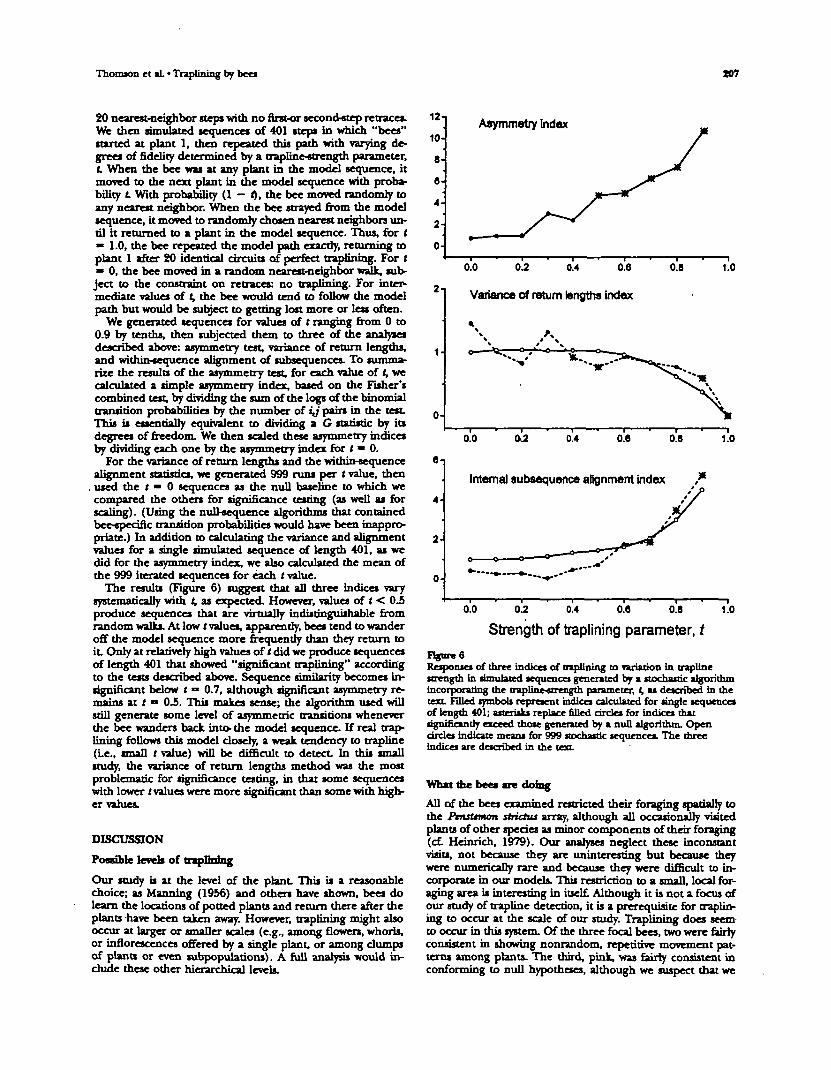
We generated sequences for values of t ranging from 0 to0.9 by tenths, then subjected them to three of the analysesdescribed above: asymmetry test, variance of return lengths,and within-cequence alignment of subsequences. To summa-rize the results of the asymmetry test, for each value of t, wecalculated a simple asymmetry index, based on the Fisher'scombined test, by dividing the sum of the logs of the binomialtransition probabilities by the number of ij pairs in the test.This is essentially equivalent to dividing a G statistic by itsdegrees of freedom. We then scaled these asymmetry indicesby dividing each one by the asymmetry index for t • 0.

For the variance of return lengths and the within-sequencealignment statistics, we generated 999 runs per (value, then

. used the t • 0 sequences as the null baseline to which wecompared the others for significance testing (as well as forscaling). (Using the null-sequence algorithms that containedbee-specific transition probabilities would have been inappro-priate.) In addition to "»''~vl?^r|g the variance and alignmentvalue* for a single simulated sequence of length 401, as wedid for the asymmetry index, we also calculated the mean ofthe 999 iterated sequences for each tvalue.

The results (Figure 6) suggest that all three indices varysystematically with t, as expected. However, values of ( < 0.5produce sequences that are virtually indistinguishable fromrandom walks. At low t values, apparently, bees tend to wanderoff the model sequence more frequently than they return toit. Only at relatively high values of t did we produce sequencesof length 401 that showed "significant traplining" accordingto the tests described above. Sequence similarity becomes in-significant below t•> 0.7, although significant asymmetry re-mains at t — 0.5. This makes sense; the algorithm used willstill generate some level of asymmetric transitions wheneverthe bee wanders back into- the model sequence. If real trap-lining follows this model closely, a weak tendency to trapline(Le., small t value) win be difficult to detect. In this smallstudy, the variance of return lengths method was the mostproblematic for significance testing, in that some sequenceswith lower t values were more «ignlfir-ant than some with high-er values.

DISCUSSION

Possible levels of trapBnmg

Our study b at the level of the plant This is a reasonablechoice; as Manning (1956) and others have shown, bees dolearn the locations of potted plants and return there after theplants have been taken away. However, traplining might alsooccur at larger or smaller scales (e.g., among flowers, whorls,or inflorescences offered by a single plant, or among dumpsof plants or even subpopulations). A full analysis would in-clude these other hierarchical levels.

12-

10-

8

6

4

2

0-1

Asymmetry index

1-

0-

0.0 0.2 0.4 0.6

Variance of return lengths index

0.8 1.0

0.0 &2 0.4 0.8 0.8 1.0

e-i

Internal subsequence aSgnment index

0.0 0.2 0.4 o.e 0.8 1.0

Strength of traplining parameter, f

F|£U1'G 6

Responses of three indices of traptining to variation in traplinestrength in shmihrrd sequence! generated by a stochastic algorithmincorporating the trapline-strength parameter, t, as described in thetext. Filled symbob represent indices calculated for single sequencesof length 401; asterisks replace filled circles for indices thatsignificantly exceed those generated by a null algorithm. Opencircles indicate mean* for 999 stochastic sequences. The threeIndices are described in the text.

What the bees are doing

All of the bees examined restricted their foraging spatially tothe PmsUmon strictus array, although all occasionally visitedplants of other species as minor components of their foraging(c£ Heinrich, 1979). Our analyses neglect these inconstantvisits, not because they are uninteresting but because theywere numerically rare and because they were difficult to in-corporate in our models. This restriction to a small, local for-aging area is interesting in itself. Although it is not a focus ofour study of trapline detection, it is a prerequisite for traplin-ing to occur at the scale of our study. Traplining does seem-to occur in this system. Of the three focal bees, two were fairlyconsistent in showing nonrandom, repetitive movement pat-terns among plants. The third, pink, was fairly consistent inconforming to null hypotheses, although we suspect that we

208 Behavioral Ecology VoL 8 No. 2

could have detected significant patterning of her movementswith larger data sets.

We do not know whether bumble bees usually trapline. Be-cause many observations are needed, one can detect it onlyin plant specie* that receive high visitation; these species prob-ably have unusual reward amounts or schedules. There arealso observational biases. In choosing a focal bee for accu-mulating a large data set, it is natural to choose one that isfrequently seen. Many of the bees that we marked in the Ptn-sttwvm array were not seen again. Marking trauma may havedriven them off, but they may also have been non-trapliningvagabonds. However, other studies (Thomson, 1996; ThomsonJ and Williams N, in preparation) reinforce our conclusionsthat Bombus flavifrvns on PensUmon strittus frequently foragesimilarly to Bombus Urnariui on Aratia faspida (Thomson,1988; Thomson et aL, 1982, 1987). The foraging areas aresimilar, (about 100 m1), the circuit times are similar (about10-15 min) and the sharing of plants by many bees is similar.In both cases, bees make three to four passes through thearray on one foraging trip from the nest. Additionally, weknow that on Aratia, bees gradually move their foraging areasinto areas where floral rewards are higher. It appears that beesvisit a core set of plants on virtually every pass through thearray, but they also occasionally sample other plants. If thoseplants prove rewarding, they are more likely to be visited ona subsequent pass (Thomson et aL, 1982, 1987). We suspectthat bees on Ptnsttwum do something similar (Thomson,1996).

If so, there is no reason to expect perfect traplining; in-deed, it would be pathological Rather, traplining probablypresents a special case of the common situation where animaUneed to learn information about their environment and re-member it for awhile, but also to forget it when it loses cur-rency (Mangel, 1990; Thomson, 1996). Occasional samplingis probably highly advantageous in a world where plantschange in value through time, but it will blur the conservativevisitation pattern that must underlie traplining. Therefore, westress the need for techniques that establish the reality of thatunderlying pattern.

Comparisons of methods

We have proposed several different tests of traplining. Eachof these illuminates a different aspect of potentially repeti-tious movement patterns among fixed stations. Each can thusbe viewed as a different operational definition of traplining.Prospective users should select tests, or devise new ones, thatare relevant to the biological situation and compatible withthe data. Here, we consider some of the properties of our teststhat such users should bear in mind.

Asyrnmstry testThe asymmetry test, which was developed to test for direc-tional migration (Sokal, 1991) is die only one that comparesdata to a simple statistical distribution (i.e., binomial expec-tation). It is readily grasped and shows an important aspectof nonrandomness in interstation moves, and its applicationallows the construction of the trapline skeleton diagrams,which we find useful. The index derived from this test alsoresponds to a wider range of (values than the other indices(Figure 6). The test is rather far from the essence of traplin-ing, however. It would also be blind to commuting traplining,in which a bee might go back and forth along a particularroute, ft does not serve to define traplining, but it is a usefuladjunct to other measures.

By expressing sequence data as a transition matrix, we drawattention to the role of Markov models as possible descriptorsof trapline*. C H. Janson (unpublished manuscript) has ex-

tensively analyzed traplining from a Markovian view, so herewe will cite a few points. For example, perfect traplining of asubset of plants in an array would result in a nonergodic Mar-kov chain: in such a <•*»»•". some destinations are neverreached and the effect of the starting position is never dissi-pated, as happens in the more frequently modeled ergodiccondition. Our analysis of individuality of transitions via con-tingency able could be seen as a special case or subset of aMarkov analysis; for example, our analysis could be extendedto consider whether bees' departure directions from particu-lar plants depended not only on the plant of departure (first-order Markov process) but on the preceding plant as well(second-order process). Janson (personal communication)shows that the movements of a monkey troop cannot be de-scribed a first-order Markov process, which he interprets asevidence for a cognitive spatial map.

NuUmoddsAside from the asymmetry test, our measures fall into two cat-egories. Some compare animal* to animal*, others compareanimaU to null models. Each type has characteristic shortcom-ings. As mentioned above, random null models are unrealisticunless we temper pure randomness with additional biologicalconstraints. If we do add constraints, our choice of constraintsbecomes part of die operational definition, and someone whomakes different choices will reach different conclusions aboutthe strength of traplining. For example, we built in an aver-sion to retraces, but we considered only one- and two-stepretraces. This decision was based on years of watching beeson many host plants and acquiring die strong impression thatsuch short retraces are so rare—so "unnatural" for bumblebees in general—that we should not permit our null bees tomake them freely. We could have gone further, also constrain-ing three-step, four-step, and all higher retraces so that theytoo would occur as often in our null sequences as in the ob-served data. Similarly, rather than choosing a destinationplant randomly from the eligible members of a chosen neigh-bor class, we could have made the null bees more likely to goto members with more flowers. At some point, however, wewould have to constrained our null sequences that they wouldhave aM the properties of die observed data. To be useful, anull model has to fall into a window of credibility: if we useunconstrained randomness, we will always reject the null, butthe rejection wiH not constitute traplining. If we constrain toocompletely, we will never reject the null, and no behavior canconstitute traplining. Anyone who chooses the null model ap-proach must also choose the constraints and be able to defendthose choices.

With that caveat registered, we suggest that die best prac-tical index or measure of traplining for our study is that basedon the variances of returns. It uses data fairly efficiently, iscomparatively easy to understand, allows a significance test,and also produces a comprehensible index of die strength oftraplining. On die other hand, it is somewhat removed fromdie ideal definition of traplining in that it does not look di-rectly at sequence similarity. If sequences are similar, returnslengths will be similar, but return lengths could conceivablybe similar without much sequence similarity. Furthermore,the weak performance of significance tests on long sequencesgenerated with various values of t is a concern.

The technique closest to die ideal definition of traptiningis the comparison of similarity (alignment) of repeated cycleswithin sequences. Its only real drawback is a serious •ne, itsdependence on long, continuous observations. Given that -null sequences must match die observed sequence (they muststart at the tame plant, be of die same length), it is hard tocombine data from different sequences, and only the longestof our sequences have two or more full cycles. Given that few

Tbonuon et aL •TrapHning by beet 109

will be easier to observe than bumble bees, this tech-nique will find little application unless » way is developed touse shorter cycles, perhaps by some objective paste-togethertechnique.

Spectral analysis of displacements is a powerful way tosearch for periodicities in the bee's spatial position, but it ismore suited for analyzing a few long sequences in depth thanfor measuring traplining strength. The product of spectralanalysis (the periodogram) is essentially just a transformationof the data from the time domain to the frequency HnmamIt is therefore as complicated as the original data series itselfand does not provide any single parameter that naturallyserves as a summary statistic We recommend spectral analysisof displacement data u an informative way to examine data,but it should always be accompanied by drawing maps of theflight paths, which may be just as informative. It seems to havelittle to contribute to the search for a general operationaldefinition of traplining, and like all of the null model ap-proaches, it depends on the assumptions built into the nullmodel.

Comparing bees to each other rather than to "random-ness" neatly evades the problem of arbitrary assumptions.However, it skips the most fundamental question, Are beesrepeating sequences? and jumps to what would logically be asecond question, Given that bees show consistent movementpatterns, are their patterns individualistic? This question givesinformation about traplining only if we reject the null hy-pothesis of homogeneity among bees. If we succeed in show-ing that different bees make consistently different moves atcertain stations, we can consider that as evidence of traplin-ing: consistent differences between bees cannot arise withoutconsistency within bees. However, if bees are basically doingthe same thing, we cannot tell whether they are traplining ornot In our case, both contingency tables and the Mantel testjn^'catr that bees do differ, both in their decision-making atparticular points in the array and in the similarity of their'sequences. A limitation common to both of these methods isthe requirement that the bees' foraging areas overlap to someextent

Of these two approaches, the Mantel test seems closer tothe essence of traplining because it examines sequences. Onthe other hand, it is a less fatnfKar approach than contingencytables. Also, although we have not explored the test's behaviorfully, the overall Mantel results seem rather volatile. FJiminat-ing only a few sequences, perhaps 5% of the total, can changethe matrix correlation from highly significant to insignificantUntil a more systematic sensitivity analysis has been complet-ed, including an examination of alternative similarity mea-sures, we would be reluctant to recommend this approach.Contingency tables seem adequate for testing individuality, al-though our use of separate tables and Fisher's combinedprobabilities test is less elegant than Janson's (1996; unpub-lished data) approach to the same question using Markovmodels.

*^" IiniHrSf*piiff of toff t r n y

In the search for statistical signatures of traplining, we re-peatedly encounter a requirement for large data sets. Thefour focal bees were obviously far from being pure, regulartrapliner*; indeed, several tests support the conclusion thatpink was not traplining. The other bees were irregularenough that only by compiling many observations could wefind various sorts of repetitive patterns in their movements. Itmakes sense that we cannot recognize a trapline as a repeatedpattern unless we have seen an animal traverse it numeroustimes during a long slice of time. This leads to a dilemma:statistically, traplines are a moving target

We know from other studies (Thomson et aL, 1982, 1987)and from the comparison of blue early with blue late in thisstudy, that the foraging areas of bumble bees change throughtime. This is accomplished by adding some new plants to theroute while deleting others. Rapid trapline drift will mean thatthe first sequences in a long data set may resemble the lastones so weakly that the hypothesis of traplining is rejected,even though the animal's route has evolved only throughgradual, incremental change. Gradual evolution of this sort isdifferent from sloppy repetition of a basically fixed cycle, butour techniques will not make the distinction: both processeswiD weaken traplining. I£ for example, we had pooled theearly and late data sets for bee blue, several indications thatwere significant in each separate data set may have been in-significant in the whole. This is essentially a stationarity prob-lem, and we have no tested solution to offer. Given enoughdata, one could gauge the problem by ordinating sequencesby the alignment-similarity matrix, then connecting the pointsfor each bee's sequences in temporal order. If the resultingtraces form small, nonoverlapping clusters, trapline driftshould pose no problem for detecting individuality. If the trac-es are long, intertwining with others, then stationarity may be

It is also evident that observers should strive to get sequenc-es that are as long as possible. Although short fragments ofsequences can be useful for analyses based on the transitionmatrix, other techniques, such as spectral analyses and align-ment of cycles within sequences, depend on long records.These methods will not be useful for animal* that cannot befollowed for long bouts. This brings up another unfortunatetrade-off. Our restricted array was designed to ease observa-tion. Working in a much larger natural stand, with irregularplant spacing, would make it harder to maintain continuousrecords, as bees are more easily lost on longer flights. On theother hand, a larger stand would make it much easier fortechniques such as displacement series to distinguish traplin-ing bees from more random foragers. In an infinite stand, anon-traplining bee could potentially drift away from its start-ing point without limit, more like a true random walk (Kareivaand Shigessada, 1983). In our case, a bee that limited itself toPtnsttmon strictiu could drift no farther than a few meters.Such bees necessarily retrace their steps frequently (Figure 4),mating it harder to distinguish traplining from constrainednull movement

Using a small array highlights another elusive distinction.We could imagine a bee that uses the entire array by passingthrough it in a repeatable sequence—an indubitable trapliner.We can also imagine a bee that restricts itself to only half thearray, but within that half shows no more repetition thanwould be expected from a null process. (See the blue late dataset. Figure 3.) Both of these bees would show significant trap-lining according to our tests that compare them to null beesusing the entire array. This does not seem desirable, but thereis no clear way to fix the problem. To satisfy our curiosity, wereanalyzed the blue late data, using null models in which visitswere allowed only to plants 1-9, 11-15, and 19-21. (We alsopurged die observed data of the single visit to plant 27 thatstarted one sequence.) As expected, the deviation of the ob-served data from the null models weakened. For the varianceof returns test, die Fisher combined significance level de-clined from .001 to .025; for the alignment of sub-sequencestest, it remained rnsignifiram at JS < p < .1.

It seems, then, that significant regularity remains within thisdata set even when the array is collapsed to include only thoseplants that the bee actually frequented. This "fix-up" evadesthe crux, however. Why draw the line at plants that are nevervisited? Why not further condition the null bee to visit plantsin the same proportion as die observed bee? Because thu

210 Behavioral Ecology VoL »

would eliminate a principal feature of trapliner the freedomof a bee to move preferentially to tome plants rather thanothers. If an observed bee always avoided one particular plantwhile visiting those all around it, we would consider that avoid-ance part of its regular route, part of the selectivity that de-fines traplining. We would not constrain null bees to avoid italso. Although this case may seem different from the type ofselectivity shown by blue late, the difference is one of scaleand the distinction is gray rather than black and white. Thereis no way to deconfound avoidance of plants from avoidanceof foraging areas as sources of non-randomness. This is an-other reason why the null model comparisons are arbitrary:they demand assumptions about the available foraging arenaas well as about movement rules. For this reason, again, thebetween-bee comparisons are necessary adjuncts to the nullmodels.

Overall, no single method provides a complete solution tothe operational definition of traplining. If the goal is to doc-ument that animal* are showing statistically irgn •"<•")? regu-larities in their repeated passes through an array of stations,it is probably best to apply as many methods as possible, witheach test contributing its unique increment to a general di-agnosis. More often and more usefully, model selection willbe guided by an adaptive analysis of the problem facing theanimal An investigator might ask what sort of repetitive for-aging patterns one might expect from bees using a particulartactic or facing a particular spatial problem. Then, one shouldselect a test that is appropriate to the properties of the data(e.g., sequence length) and the question. We hope that thesuggestions here provide a starting point.

We thank Andrea Lowrance, l i s t Rigney, and George Wdblen forfield attltrance. Useful dltniition has been contributed by too manycolleague* to name, but Ralph Cartar, Charles Janson, and Neal Wil-liam* ttand out Manuscript preparation wa* funded by the NationalScience Foundation (IBN 9316792 and a Mid-Career Fellowihip toJJXT.) and eased by the hospitality of of the Hatting* Reservation andthe Integradve Biology Department at the University of California,Berkeley. This is contribution 971 in Ecology and Evolution, SUNY-Stony Brook.

REFERENCES

Ackennan DJ, Metier MR, Lu EL, Montalvo AM, 1982. Food-foragingbehavior of male euglossmin (Hymenoptera: Apidae): vagabondsor traplinen? Biotropfca 14:241-248.

Anderson DJ, 1983. Optimal foraging and the traveling nlnmsn.Theor Popul Biol 24:145-159.

Freeman RB, 1968. Charles Darwin on the routes of male humblebees. BuH Br Mus Nat Hist Hist Ser 3:177-189.

Garber PA, 1988. Foraging decisions during nectar feeding by tamarin

monkeys (Scgmtus mystax and Sagumus fusdcoltu.Primates) in Amir on tan Peru. Biotropka 20:100-106.

Gill FB, 1988. Trapline foraging by hermit hummingbirds: competi-tion for an undefended, renewable resource. Ecology 69:1933-1942.

Hdnrich B, 1976. The foraging specializations of individual bumble-bees. Ecol Monogr 46:105-128.

Heinrich B, 1979. "Majoring" and "mlnoring" by foraging bumble-bees, Bombus vaganx an experimental analysis. Ecology 60:245-255.

Janson CH. 1996. Toward an experimental socioecology of primates:examples from Argendne brown capuchin monkeys (Cc6ui nptttnlagritus) In: Adaptive radiations of neotropical primates (NorconkR, Rosenberger A, Garber P, eds). New Ybrfc Plenum Press.

DH 1971 F l \ tigical plants. Science 171203-205.

Kareiva PM, Shigessada N, 1983. Analyzing insect movement as a cor-related random walk. Oecologia 56334-238.

Mangel M, 1990. Dynamic information in imcer****1 and changingworlds. J Theor Biol 146J17-332.

Manning A, 1956. Some aspects of the foraging behaviour of bumble-bees. Behaviour 9:164-201.

Mantel N, 1967. The detection of disease clustering and a generalizedregression approach. Cancer Research 27209-220.

Milton K, 1981. Distribution patterns of tropical plant foods as anevolutionary stimulus Co primate mental development. Am Andiro-pol 83:535-643.

Morse DH, 1982. Behavior and ecology of bumble bees. In: Socialinsects, voL m (Hermann HR, ed). New Vforfc Academic Press.

Proctor M, Tfeo, P, Lack A, 1996. The natural history of pollination.London: HarperCollins.

Pyke GH, 1978. Optimal foraging: movement patterns of bumblebeesbetween inflorescences. Theor Popul Biol 13:72-98.

Sokal RR, 1979. Taring significance of geographic variation pattern*.Syst Zool 28227-231.

Sokal RR, 1991. Ancient movement patterns determine modern ge-netic variances in Europe. Hum Biol 63:589-606.

Sokal RR, Rohlf FJ, 1995. Biometry. San Frandsco, California: W. H.Freeman.

Thomson JD, 1988. Effects of variation in inflorescence size and floralrewards on the visitation rates of traplining pollinators of AraBakupida. Evol Ecol 2:65-76.

Thomson JD, 1996. Trapline foraging by bumble bees: L Persistenceof flightrpath geometry. Behav Ecol 7:158-164.

Thomson JD, Harder LD, Peterson SC, 1987. Response of trapliningbumble bees to competition experiments: shifts in feeding locationand efficiency. Oecologia 71295-300.

Thomson JD, Maddison WP, Pkmright RC, 1982. Behavior of bumblebee pollinator* of Araha laspida Vent (Anliaceae). Oecologia 54:326-336.

Ttnbergen N, 1968. Curious nfy? 1 1*" Garden dry, New Jersey: An-chor Books.

Waterman MS, 1989. Mathematical methods for DNA sequences. BocaRaton, Florida; CRC Press.

Wilkinson L, 1990. SYSTAT: the system for statistics. Evanston, Illinois:Systat, Inc.