Embed Size (px)
Citation preview
Behaviour modelling of Wideband - Code Division Multiple Access
By: Jack Huynh & Mattias Gylin
LITH-ISY-EX-3731-2005
Linköping 2005-03-18
Master Thesis on
Behaviour modelling of Wideband - Code Division Multiple Access
By: Jack Huynh & Mattias Gylin
LITH-ISY-EX-3731-2005
2005-03-18
Supervisor: Anders Nilsson
Department of system engineering (ISY) at the University of Linköping
Examiner: Dake Liu Department of system engineering (ISY)
at the University of Linköping
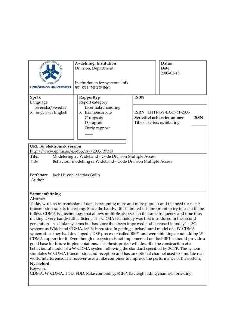
Avdelning, Institution Division, Department Institutionen för systemteknik 581 83 LINKÖPING
Datum Date 2005-03-18
Språk Language
Rapporttyp Report category
ISBN
Svenska/Swedish X Engelska/English
Licentiatavhandling X Examensarbete
ISRN LITH-ISY-EX-3731-2005
C-uppsats D-uppsats
Serietitel och serienummer Title of series, numbering
ISSN
Övrig rapport ____
URL för elektronisk version http://www.ep.liu.se/exjobb/isy/2005/3731/
Titel Title
Modelering av Wideband - Code Division Multiple Access Behaviour modelling of Wideband - Code Division Multiple Access
Författare Author
Jack Huynh, Mattias Gylin
Sammanfattning Abstract Today wireless transmission of data is becoming more and more popular and the need for faster transmission rates is increasing. Since the bandwidth is limited it is important to try to use it to the fullest. CDMA is a technology that allows multiple accesses on the same frequency and time thus making it very bandwidth efficient. The CDMA technology was first introduced in the second generation’s cellular systems but has since then been improved and is reused in today’s 3G systems as Wideband CDMA. ISY is interested in getting a behavioural model of a W-CDMA system since they had developed a DSP processor called BBP1 and were thinking about adding W-CDMA support for it. Even though our system is not implemented on the BBP1 it should provide a good base for future implementations. This thesis project will describe the construction of a behavioural model of a W-CDMA system following the standard specified by 3GPP. The system simulates W-CDMA transmission and reception and has an optional channel used to simulate real world interference. The receiver uses a rake combiner to improve the performance of the system. Nyckelord Keyword CDMA, W-CDMA, TDD, FDD, Rake combining, 3GPP, Rayleigh fading channel, spreading
i
Contents 1 INTRODUCTION ....................................................................................................................................... 1
1.1 TARGET READER................................................................................................................................... 1 1.2 READING INSTRUCTIONS....................................................................................................................... 1 1.3 CELLULAR PHONE SYSTEM BACKGROUND ............................................................................................ 2 1.4 IMPORTANT DEFINITIONS ...................................................................................................................... 6
2 PROBLEM DESCRIPTION ...................................................................................................................... 8 2.1 MOTIVATION ........................................................................................................................................ 8 2.2 AIMS AND OBJECTIVES.......................................................................................................................... 8 2.3 CONSTRAINS AND ASSUMPTIONS .......................................................................................................... 9 2.4 REQUIREMENTS .................................................................................................................................... 9
3 BACKGROUND THEORY...................................................................................................................... 11 3.1 CYCLIC REDUNDANCY CHECK (CRC) ................................................................................................ 11 3.2 INTERLEAVER ..................................................................................................................................... 11 3.3 MODULATION ..................................................................................................................................... 12 3.4 SPREADING ......................................................................................................................................... 14
3.4.1 Advantages of using spreading...................................................................................................... 14 Multiple access ......................................................................................................................................................... 15 Protection against multipath interference ................................................................................................................. 15 Privacy...................................................................................................................................................................... 15 Interference rejection................................................................................................................................................ 15 Anti-jamming capability........................................................................................................................................... 16 Low probability of interception ................................................................................................................................ 16
3.4.2 Spreading theory ........................................................................................................................... 16 3.4.3 Spreading codes ............................................................................................................................ 20
Channelisation codes ................................................................................................................................................ 20 Orthogonality of channelisation codes ..................................................................................................................... 21 Scrambling sequence ................................................................................................................................................ 22
3.4.4 Spreading data .............................................................................................................................. 22 3.4.5 Despreading data .......................................................................................................................... 23
3.5 FRAMES AND TIMESLOTS STRUCTURE ................................................................................................ 26 3.5.1 Midamble ...................................................................................................................................... 26 3.5.2 Frames in 3.84Mcp ....................................................................................................................... 26 3.5.3 Timeslots in 3.84Mcp .................................................................................................................... 26 3.5.4 Frames in 1.28 .............................................................................................................................. 27 3.5.5 Timeslots in 1.28Mcp .................................................................................................................... 27
3.6 SYNCHRONISATION CODES FOR 3.84MCP ........................................................................................... 28 3.6.1 Primary Synchronisation Code (PSC) .......................................................................................... 29 3.6.2 Secondary synchronisation code ................................................................................................... 29
3.7 PULSE-SHAPING .................................................................................................................................. 30 3.8 MULTIPATHS....................................................................................................................................... 31 3.9 RAKE COMBINER................................................................................................................................. 32
4 SYSTEM OVERVIEW ............................................................................................................................. 34 4.1 DATA GENERATOR.............................................................................................................................. 36 4.2 CRC ................................................................................................................................................... 36 4.3 INTERLEAVER ..................................................................................................................................... 36 4.4 MODULATION ..................................................................................................................................... 36 4.5 SPREADING ......................................................................................................................................... 36 4.6 CREATING SLOTS ................................................................................................................................ 37
ii
4.6.1 Timeslots 3.84Mcp ........................................................................................................................ 37 4.6.2 Timeslots 1.28Mcp ........................................................................................................................ 37 4.6.3 Midamble ...................................................................................................................................... 37
4.7 SYNCHRONISATION CODES FOR 3.84MCP ........................................................................................... 38 4.8 PULSE-SHAPING .................................................................................................................................. 38 4.9 CHANNEL............................................................................................................................................ 38 4.10 RAKE COMBINER................................................................................................................................. 38 4.11 DESPREADING..................................................................................................................................... 39 4.12 DEMODULATION ................................................................................................................................. 39 4.13 CRC-CHECK....................................................................................................................................... 39 4.14 SIGNAL TO NOISE RATIO (SNR) ......................................................................................................... 39 4.15 BIT ERROR RATE (BER) ..................................................................................................................... 39
5 IMPLEMENTATION OF THE SYSTEM.............................................................................................. 41 5.1 TRANSMITTER..................................................................................................................................... 42
5.1.1 Trans ............................................................................................................................................. 43 5.1.2 DataGen ........................................................................................................................................ 43 5.1.3 QPSK............................................................................................................................................. 44 5.1.4 Primary ......................................................................................................................................... 44 5.1.5 Secondary...................................................................................................................................... 44 5.1.6 SlotsConstructor............................................................................................................................ 45
Midamble ................................................................................................................................................................. 45 Spreading.................................................................................................................................................................. 46
5.1.7 RCosFilter ..................................................................................................................................... 50 5.1.8 Upsample ...................................................................................................................................... 50 5.1.9 Conv .............................................................................................................................................. 50
5.2 CHANNEL............................................................................................................................................ 50 5.2.1 Channel ......................................................................................................................................... 51 5.2.2 MyChannel .................................................................................................................................... 51 5.2.3 writeToMFile................................................................................................................................. 52 5.2.4 Calling the channel program ........................................................................................................ 52
5.3 RECEIVER ........................................................................................................................................... 53 5.3.1 SignalReceiver............................................................................................................................... 54
Determining a threshold value.................................................................................................................................. 54 Finding primary synchronization signal ................................................................................................................... 55 Receiving data .......................................................................................................................................................... 55
5.3.2 Reconstruct.................................................................................................................................... 56 ChannelCode ............................................................................................................................................................ 56 ScramblingCode ....................................................................................................................................................... 56 Despreading data ...................................................................................................................................................... 56 findMultipath............................................................................................................................................................ 56 fixAngle.................................................................................................................................................................... 57 Overview of the Rake-combiner............................................................................................................................... 57
5.3.3 Primary ......................................................................................................................................... 59 5.3.4 deqpsk............................................................................................................................................ 59 5.3.5 bitErrorRate .................................................................................................................................. 59 5.3.6 writeConstellationPoints............................................................................................................... 59 5.3.7 writeToMFile................................................................................................................................. 59
6 TEST RESULTS........................................................................................................................................ 60 6.1 GOALS WITH TESTS ............................................................................................................................. 60 6.2 TESTING PROCEDURE .......................................................................................................................... 60 6.3 PRESENTING THE TEST RESULTS.......................................................................................................... 61

iii
6.4 TESTING THE SYSTEM WITHOUT THE CHANNEL................................................................................... 62 6.5 TESTING THE SYSTEM WITH THE CHANNEL ......................................................................................... 62
6.5.1 Using only 1 path .......................................................................................................................... 63 6.5.2 Using 2 or 3 paths ......................................................................................................................... 63 6.5.3 Using 4 paths................................................................................................................................. 64 6.5.4 Using 5 or 6 paths ......................................................................................................................... 68
6.6 SUMMARY .......................................................................................................................................... 68 7 CONCLUSION AND FUTURE DEVELOPMENT............................................................................... 70
7.1 REQUIREMENTS FULFILLED................................................................................................................. 70 7.2 FUTURE DEVELOPMENT ...................................................................................................................... 71
Appendix A – References..................................................................................................... 73
Appendix B – User manual .................................................................................................. 75
Appendix C – Classes and Functions ................................................................................ 77
Appendix D – Abbreviation................................................................................................... 91
Appendix E – Technical Terms ........................................................................................... 92
Appendix F – Matlab version ............................................................................................... 94
Appendix G – Workload ........................................................................................................ 95
iv
List of Figures Figure 1-1: FDMA vs. TDMA vs. CDMA................................................................................. 3
Figure 1-2: TDD and FDD transmission.................................................................................... 4
Figure 1-3: Ideal cell structures for 3-, 4- and 7-cells clusters................................................... 5
Figure 1-4: 7-cells reuse clusters................................................................................................ 6
Figure 3-1 : Blockinterleaver of size 3x4................................................................................. 12
Figure 3-2: The left picture is an example of constellation points for QPSK modulation and the right is an example of constellation points for 16-QAM modulation. ....................... 13
Figure 3-3: Mapping of natural order and grey coded labelling schemes................................ 13
Figure 3-4: 16-QAM modulation errors with different schemes ............................................. 14
Figure 3-5: The despreading operations effect on signals and interference............................. 15
Figure 3-6: The effect on interference on the transmitted signal. ............................................ 16
Figure 3-7 : Fourier transform of a rectangle pulse. ................................................................ 17
Figure 3-8 : Spectrum of the unspread signal. ......................................................................... 17
Figure 3-9 : Spectrum for the signal used for spreading. ........................................................ 18
Figure 3-10 : Result of the spreading operation in the frequency domain. .............................. 19
Figure 3-11 : Scaled version of Figure 3-10. ........................................................................... 19
Figure 3-12: Method for generating channelisation codes....................................................... 20
Figure 3-13: Spreading data. .................................................................................................... 22
Figure 3-14: The effect of spreading........................................................................................ 23
Figure 3-15: Despreading data. ................................................................................................ 24
Figure 3-16: Despreading the signal with the correct spreading code. .................................... 25
Figure 3-17: Despreading the signal with an orthogonal spreading code. ............................... 25
Figure 3-18: Frame structure for 3.84Mcp............................................................................... 26
Figure 3-19: Timeslot structure for 3.84Mcp........................................................................... 27
Figure 3-20: Frame structure for 1.28Mcp............................................................................... 27
Figure 3-21: Timeslot structure for 1.28Mcp........................................................................... 27
Figure 3-22: Placement of synchronisation codes.................................................................... 28
Figure 3-23: Result of when a PSC is found while despreading the received data.................. 29
Figure 3-24: RCOS filter.......................................................................................................... 30
Figure 3-25: The effect of filtering the signal with a RCOS filter. .......................................... 31
v
Figure 3-26: The left diagram is the absolute value of the signal sent and the right diagram is the signal with its multipath. ............................................................................................ 32
Figure 3-27: The energy of the data signal, path from transmission via the channel to after the rake combiner. .................................................................................................................. 33
Figure 4-1: System structure. ................................................................................................... 35
Figure 4-2 : QPSK mapping scheme for the system. ............................................................... 36
Figure 5-1: system overview.................................................................................................... 41
Figure 5-2: Blocks for classes and functions. .......................................................................... 42
Figure 5-3: Transmitters structure............................................................................................ 43
Figure 5-4: Spreading the data symbols. .................................................................................. 49
Figure 5-5: Channel structure................................................................................................... 51
Figure 5-6: How the channel works. ........................................................................................ 52
Figure 5-7: Structure of the receiver. ....................................................................................... 54
Figure 5-8: Threshold value. .................................................................................................... 55
Figure 5-9: How synchronization is performed in the system. ................................................ 56
Figure 5-10: a) Peaks from three PSC before channel b) Peaks from the three PSC after the channel. ............................................................................................................................ 57
Figure 5-11: Example of a rake with 4 fingers......................................................................... 58
Figure 5-12: a) Original modulated data, b) phase and amplitude shifted multipaths of the original constellation point, c) reconstructed data from multiple constellation points. .. 59
Figure 6-1: Constellation points for the case without interference. ......................................... 62
Figure 6-2: Constellation points of the 4 multipath/4 rake finger case with no noise added... 65
Figure 6-3: Constellation points of the 4 multipath/4 rake finger case with some noise added. SNR = 1.5......................................................................................................................... 66
Figure 6-4: Constellation points of the 4 multipath/4 rake finger case with much noise added. SNR=-8.1.......................................................................................................................... 67
Figure 6-5: The relation between the number of bit errors and the SNR................................. 68
vi
List of Tables Table 3-1: Channelisation codes. ............................................................................................. 21
Table 5-1: Multipliers for the channelisation code. ................................................................. 47
Table 5-2 : Scrambling code 0. ................................................................................................ 48
Table 5-3: Example of channel specifications. ........................................................................ 51
Table 6-1: Test cases. ............................................................................................................... 61
Table 6-2: Test parameters for the case with 1 path. ............................................................... 63
Table 6-3: Test parameters for the case with 2 or 3 paths........................................................ 63
Table 6-4: Test parameters for the case with 4 paths. .............................................................. 64
Table 6-5: Test parameters for the case with 5 or 6 paths........................................................ 68
Table 6-6: First error occurrence.............................................................................................. 69
Table 7-1: Mandatory requirements fulfilment ........................................................................ 70
Table 7-2: Optional requirements fulfilment ........................................................................... 71
vii
Abstract
Today wireless transmission of data is becoming more and more popular and the need for faster transmission rates is increasing. Since the bandwidth is limited it is important to try to use it to the fullest. CDMA is a technology that allows multiple accesses on the same frequency and time thus making it very bandwidth efficient. The CDMA technology was first introduced in the second generation’s cellular systems but has since then been improved and is reused in today’s 3G systems as Wideband CDMA.
ISY is interested in getting a behavioural model of a W-CDMA system since they had developed a DSP processor called BBP1 and were thinking about adding W-CDMA support for it. Even though our system is not implemented on the BBP1 it should provide a good base for future implementations.
This thesis project will describe the construction of a behavioural model of a W-CDMA system following the standard specified by 3GPP. The system simulates W-CDMA transmission and reception and has an optional channel used to simulate real world interference. The receiver uses a rake combiner to improve the performance of the system.
Keywords: CDMA, W-CDMA, TDD, FDD, Rake combining, 3GPP, Rayleigh fading channel, spreading

viii
Acknowledgment We would like to take the opportunity to thank a few persons that made our master thesis work possible.
First we would like to thank our examiner who approved and gave us the chance to work on such interesting and rewarding thesis work.
Second we would like to thank our supervisors Anders Nilsson and Eric Tell, who have put up with us for six months, helping us with the problems we encountered and answered the questions raised.
Lastly we would like to thank Daniel Nilsson and Henrik Norin, our opponents, with their many many comments on our thesis paper, which most probably makes it a little easier for readers to follow what has been done in this thesis work.
Chapeter – 1 Introduction
1
1 Introduction
This chapter gives an introduction to this master thesis work, describes the readers targeted with this report, explains some important terms/definitions and contains reading instructions for the document.
1.1 Target reader The readers targeted with this report are people with a good understanding of mathematics and computer science. Some basic understanding of radio transmission and cellular phone systems is beneficial but not required. Readers with little knowledge of cellular phone systems and radio transmission should read section 1.3 and chapter 3 extra carefully.
1.2 Reading instructions The thesis will start with a brief introduction of cellular systems, section 1.3, to give the reader some background on the thesis work.
For problem description on the implemented system, read chapter 2 .
Chapter 3 explains the different parts of the system, giving the reader an overview and a better understanding of the theory behind the system. A reader with a good knowledge on CDMA transmission theory is not required to read this chapter to follow the thesis work.
Chapter 4 provides an overall overview of the system implemented.
Readers who are only interested in the implementation of the system program are refereed to chapter 5 for the actual implementations. The tests performed on the system and the test results are described in chapter 6 .
Our conclusion on the thesis work and suggestions for possible future improvements of the system can be found in chapter 7 .
In the end of the report abbreviations, references, explanations and Appendix for the report can be found. The Appendix contains class and function descriptions and a user manual.

Chapeter – 1 Introduction
2
1.3 Cellular phone system background The need to for sending large quantities of data efficiently with cellular phones has never been greater. Today’s cellular phones have become something more than just a wireless telephone. Even when the cellular phones first became common to the public through out the whole world several years ago, ~1995, they already had other uses such as clock, wakeup alarm, calendar, currency converter, notebook, calculator, and even games were available for the phones and the list goes on and on. Besides the extra features it was still only a wireless phone which was used for calling, sending/receiving SMS and even FAX. Not considering the two side features, SMS and FAX, the time it takes from sending data until receiving it wasn't crucial. The only critical data needed to be sent was sound and transmitting sound does not require very high transmission rates. Today’s cellular phones send/receive more than just sound. Today you can send/receive pictures to/from other users, call others using video calls, check emails and even surf the Internet. Some of these features require much higher data transmission rate than others. This is what the new 3G phones can provide compared to the old GSM1 phones, [1].
In the early 1980’s, when many countries deployed the first generation of cellular systems, the systems where based on FDMA2 technology [1]. The FDMA system divides the cellular frequency band into many sub-bands, each with its own carrier frequency. Each user of the system is assigned a portion of the frequency band in which it transmits its data.
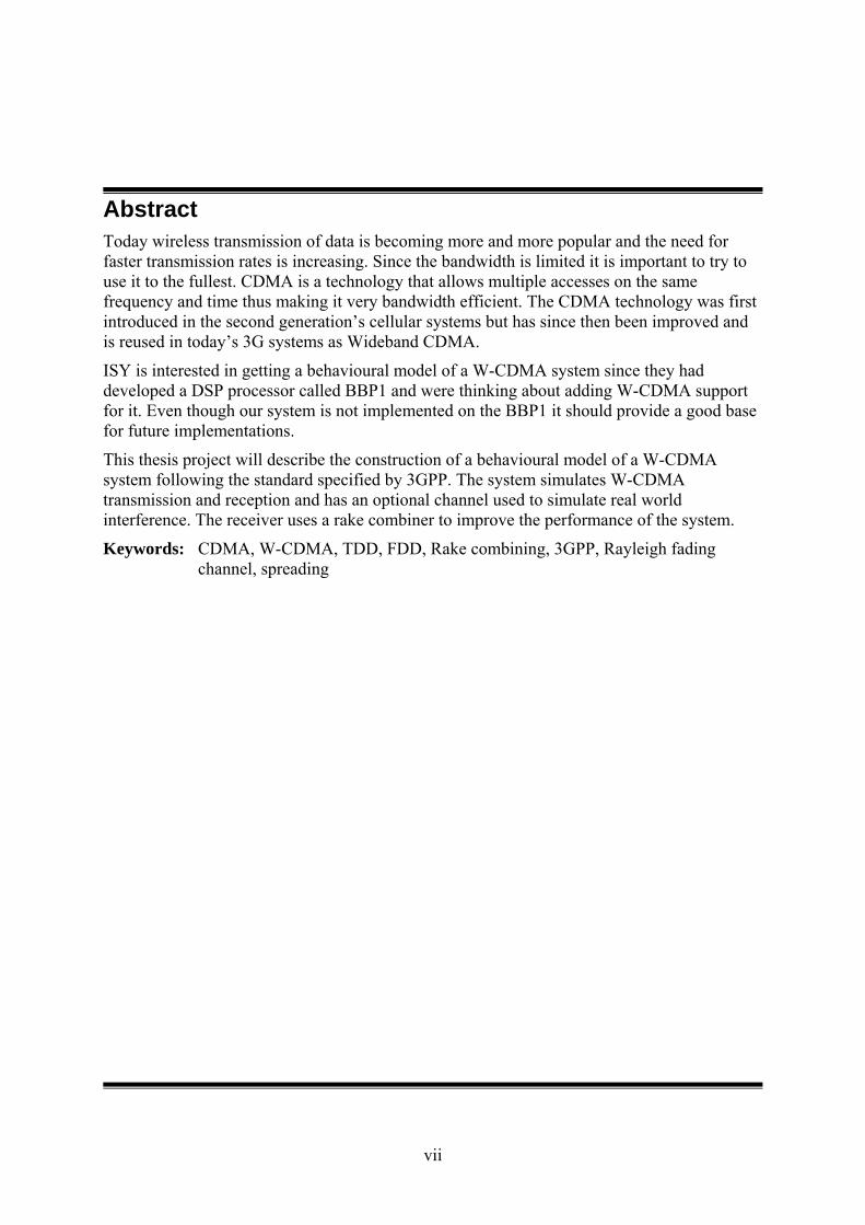
The second generation of cellular system came around 1990. During this time the cellular systems switched from analog to digital and the TDMA3 and CDMA4 technologies were introduced. In TDMA systems several users share the same frequency band, in which they transmit/receive data at clearly defined time intervals. CDMA on the other hand lets many users share the same frequency band at the time and the users are distinguished at the receiver using unique spreading codes5 [14]. Figure 1-1 illustrates the difference between these three access techniques.
1 GSM – Global System for Mobile communication 2 FDMA – Frequency Division Multiple Access. 3 TDMA – Time Division Multiple Access. 4 CDMA – Code Division Multiple Access. 5 Spreading is a way to code the data signal in CDMA. Spreading codes are used when spreading.
Chapeter – 1 Introduction
3
Figure 1-1: FDMA vs. TDMA vs. CDMA
Since the arrival of the 3G systems one multiple access standard has starting to gain popularity in Europe, W-CDMA6. W-CDMA, also known as IMT20007, was derived from the CDMA standard, which is used in both second and third generation mobile telephone systems. The original CDMA standard, also known as “CDMA one”, which is still common in the U.S. cellular telephones, offers a transmission speed of up to 14.4 Kbps in its single channel form and up to 115 Kbps in its eight-channel form. The W-CDMA standard, on the other hand, can support mobile/portable voice, images, data, and video communications at up to 2 Mbps for local area access, where users communicate with each other via one base station, or 384 Kbps for wide area access, where users communicate with each other via more then one base station [3].
There are two subgroups of W-CDMA the TDD8 and FDD9 transmission schemes. Initially FDD was the more used standard because the base station manufacturers decided to prioritize building them first, as they were deemed to be the best alternative for larger cells [2]. This means that even if the 3G-basestations did cover very large areas pretty quickly the capacity of users were limited (note that it is still very limited in some parts of Europe).
The biggest difference between FDD and TDD is that in TDD all transmission and reception to and from a user is preformed using the same frequency band. FDD on the other hand uses separate frequencies to communicate. The basic algorithm however is the same for both systems. The input signals are digitalized, encoded and spread over a larger frequency band.
6 W-CDMA – Wideband Code Division Multiple Access. 7 IMT200 – International Mobile Telecommunication 2000 8 TDD – Time Duplex Division. 9 FDD – Frequency Duplex Division
Chapeter – 1 Introduction
4
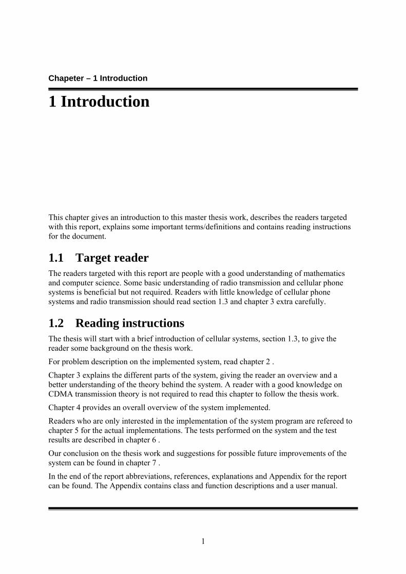
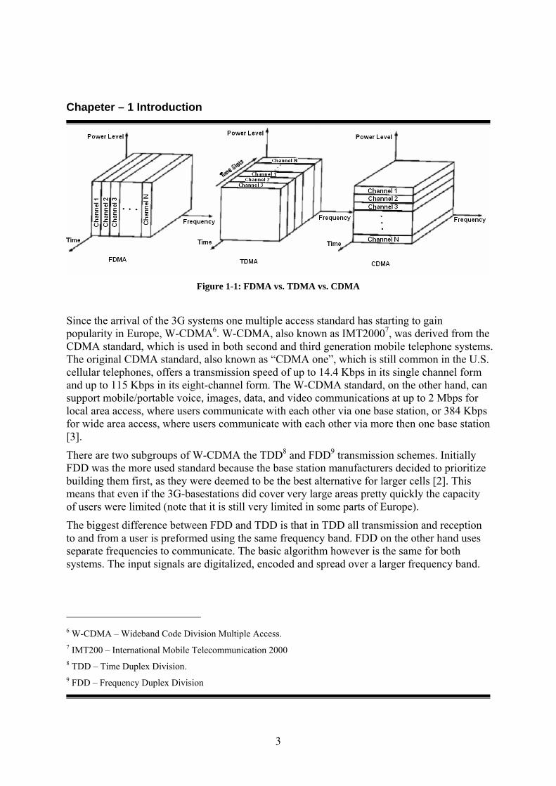
Figure 1-2 illustrates the two transmissions. The transmissions in this scheme are divided in to frames10, and each of these frames consists of several uplink and/or downlink timeslots11.
Figure 1-2: TDD and FDD transmission.
Regardless of what multiple access standard is used for a cellular phone system the basic technological components are still radio transmission and computer technology. The cellular phone system’s two main basic functions are to track and locate Base Stations (BS) and to access the best base station available. For this purpose a continuous evaluation of the connected BS radio link quality is needed. The nearby BS radio link quality is also evaluated in case there is a link with better quality than the current one then the cellular phone will consider switching base station.
Each base station has its own cover area of cellular phone users, called cell. In dense populated cities, where there are many users relative the area, there is always a shortage on frequency bands for cellular phone users. This makes the placement of BS very important because each cell has a limited frequency band at its disposal. The limitation of the frequency band also limits the number of mobile phones a cell can take care of.
Theoretically the cells are usually shaped like hexagons. But in practical there are many elements that need to be considered when forming a cell. The locations surrounding, radio shadows and the expected number of users in the area are a few of the elements. The cover 10 Frame – Larger transmission structure containing timeslots. 11 Timeslot – A structure for transmitting data in CDMA.
Timeslot
Chapeter – 1 Introduction
5
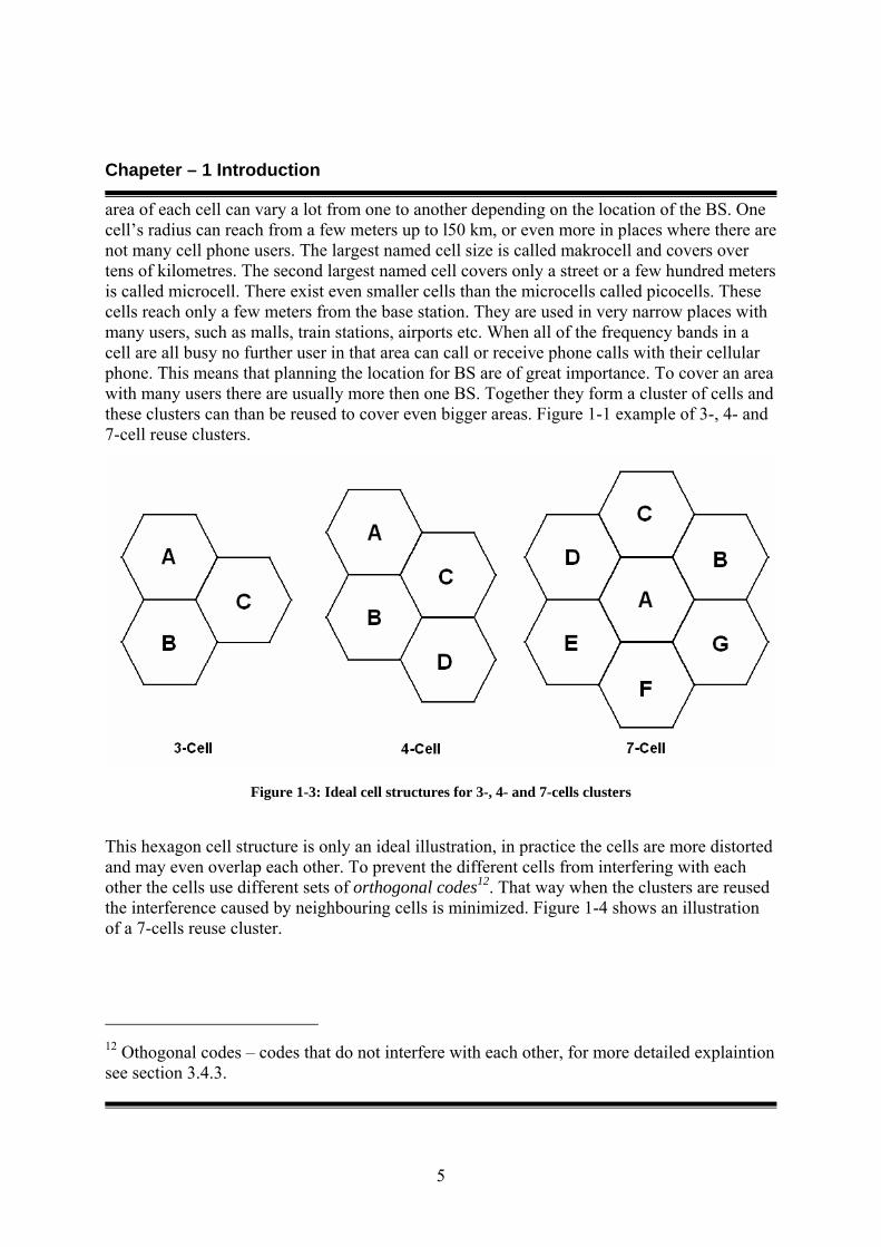
area of each cell can vary a lot from one to another depending on the location of the BS. One cell’s radius can reach from a few meters up to l50 km, or even more in places where there are not many cell phone users. The largest named cell size is called makrocell and covers over tens of kilometres. The second largest named cell covers only a street or a few hundred meters is called microcell. There exist even smaller cells than the microcells called picocells. These cells reach only a few meters from the base station. They are used in very narrow places with many users, such as malls, train stations, airports etc. When all of the frequency bands in a cell are all busy no further user in that area can call or receive phone calls with their cellular phone. This means that planning the location for BS are of great importance. To cover an area with many users there are usually more then one BS. Together they form a cluster of cells and these clusters can than be reused to cover even bigger areas. Figure 1-1 example of 3-, 4- and 7-cell reuse clusters.
Figure 1-3: Ideal cell structures for 3-, 4- and 7-cells clusters
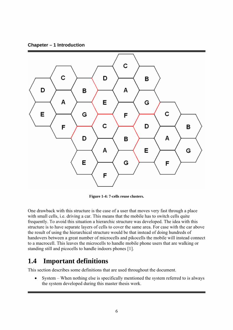
This hexagon cell structure is only an ideal illustration, in practice the cells are more distorted and may even overlap each other. To prevent the different cells from interfering with each other the cells use different sets of orthogonal codes12. That way when the clusters are reused the interference caused by neighbouring cells is minimized. Figure 1-4 shows an illustration of a 7-cells reuse cluster.
12 Othogonal codes – codes that do not interfere with each other, for more detailed explaintion see section 3.4.3.
Chapeter – 1 Introduction
6
Figure 1-4: 7-cells reuse clusters.
One drawback with this structure is the case of a user that moves very fast through a place with small cells, i.e. driving a car. This means that the mobile has to switch cells quite frequently. To avoid this situation a hierarchic structure was developed. The idea with this structure is to have separate layers of cells to cover the same area. For case with the car above the result of using the hierarchical structure would be that instead of doing hundreds of handovers between a great number of microcells and pikocells the mobile will instead connect to a macrocell. This leaves the microcells to handle mobile phone users that are walking or standing still and picocells to handle indoors phones [1].
1.4 Important definitions This section describes some definitions that are used throughout the document.
• System – When nothing else is specifically mentioned the system referred to is always the system developed during this master thesis work.
Chapeter – 1 Introduction
7
• Developers – The developers refer to the writers of this report, Mattias Gylin and Jack Huynh.
• Standard – When nothing else is specifically mentioned the standard referred to is always the 3GPP standard.
Chapeter –2 Problem description
8
2 Problem description
2.1 Motivation The purpose of the master thesis work is to create high level models of W-CDMA transmitters and receivers that will be used as a foundation to an architectural design of a processor with a matching assembler implementation of the transmitter and receiver algorithms.
At the department of system engineering, ISY, a research project is being worked on where new architectures for multi-standard base band processors are created. As a part in showing the flexibility of the processors architecture several investigations of radio standards like GSM, Bluetooth and WLAN are being performed. Since W-CDMA is the base of today’s 3G systems it’s only natural that this standard is examined too.
Designing processor architectures consist of the following steps:
1) High level implementation of transmitter and receiver algorithms.
2) Detailed choices of algorithms like synchronization, channel compensation and detection.
3) Rough hardware implementation.
4) Choice of instructions set and assembler implementation of the software.
5) Benchmarking the chosen instruction set and possibly iterations of the previous steps.
6) Implementation of processor hardware.
7) Verification.
This master thesis work purpose is to create the necessary models according to point 1 and if time allows it point 2.
2.2 Aims and objectives
Chapeter –2 Problem description
9
The aim of the thesis work is to implement a program capable of simulating the scenario of when one base station transmits data to a cellular phone. The algorithms used should follow the 3GPP standard.
2.3 Constrains and assumptions A simulation of the actual environment for a scenario when one base station transmits data to a cellular phone is impossible to implement, because there would be too many factors that needs to be taken into account. That is why some constrains and assumption about the environment of the program has been made.
• There is only one base station transmitting, meaning there will be no simulation on interference from other base stations.
• The transmission will be a one way transmission, meaning that the simulated base station will not try to receive data and that the simulated cellular phone will not try to transmit data.
• The actual radio transmission is also a program simulation, meaning that all interference on the data transmitted is added by another program.
• The signal is not multiplied with a carrier frequency before transmission since implementing such an operation is time consuming and does not provide many benefits in the simulated transmission.
• The functionality of the transmitter and the parameters for the channel are specified in the 3GPP standard but there are no specifications for the receiver. Therefore all algorithm selections and implementation of the receiver has been done by the developers themselves.
2.4 Requirements This section describes the requirements for the system developed during this thesis work. The requirements are divided into two groups; the mandatory requirements, which the system must fulfill, and the optional requirements, which should be implemented if the time schedule admits it.
Mandatory requirements R1. The system should follow the 3GPP standard.
R2. 16 Quadrature Amplitude Modulation (16-QAM) or Quadrature Phase Shift Keying (QPSK) modulation13 scheme should be supported in some way.
R3. A channel using Rayleigh fading should be implemented.
13 Modulation – Method used to map binary data onto complex values.
Chapeter –2 Problem description
10
R4. The transmitter, receiver and channel should be implemented as individual executable files.
R5. 16 bit spreading codes will be used.
R6. The final models will be implemented in C++.
R7. The system should transmit data according to TDD standard.
R8. The system should support transmitting in 3.84Mcp14 rate.
Optional requirements R9. The channel should simulate multipath15 effects and add noise.
R10. Rake combiner should be implemented.
R11. User should be able to enter a known sequence of data as transmitted data.
R12. The system should be able to transmit according to FDD standard.
R13. The system should support transmitting in 1.28Mcp rate.
R14. Implement some part of the system on a Digital Signal Processor (DSP) processor, Base Band Processor 1 (BBP1) developed by ISY16.
R15. The system shall support High Speed Downlink Packet Access (HSDPA) data
14 Mcp – Mega Chip Per second is a unit for estimating data rate in CDMA. 15 Multipath – Time delayed echo of the signal. 16 ISY – Insitutionen för SYstemvetenskap (Depart of electrical engineering)
Chapeter – 3 Background theory
11
3 Background theory
This section describes the necessary background theories needed to understand the implementation of the system created. Readers who have good knowledge about radio transmission, CDMA and computer science are not required to read this chapter.
3.1 Cyclic Redundancy Check (CRC) CRC is a method used to detect errors in the received signal. This is done by converting the binary signal to a polynomial and then dividing it with a predefined polynomial called the key. The remainder in this division is called CRC. The signal together with the CRC is transmitted. The receiver performs the same operation as the transmitter, dividing the signal with the same predefined polynomial, and checks if the remainder is zero. If the remainder is zero there is a high probability that the signal has been received correctly, otherwise an error has probably occurred, [7].
3.2 Interleaver The purpose of using an interleaver is to separate continuous bit errors. If combined with some kind error correction algorithm the system should be able to reduce the BER. There are different kinds of interleavers but the interleaver used in the 3GPP standard is the blockinterleaver, [11].
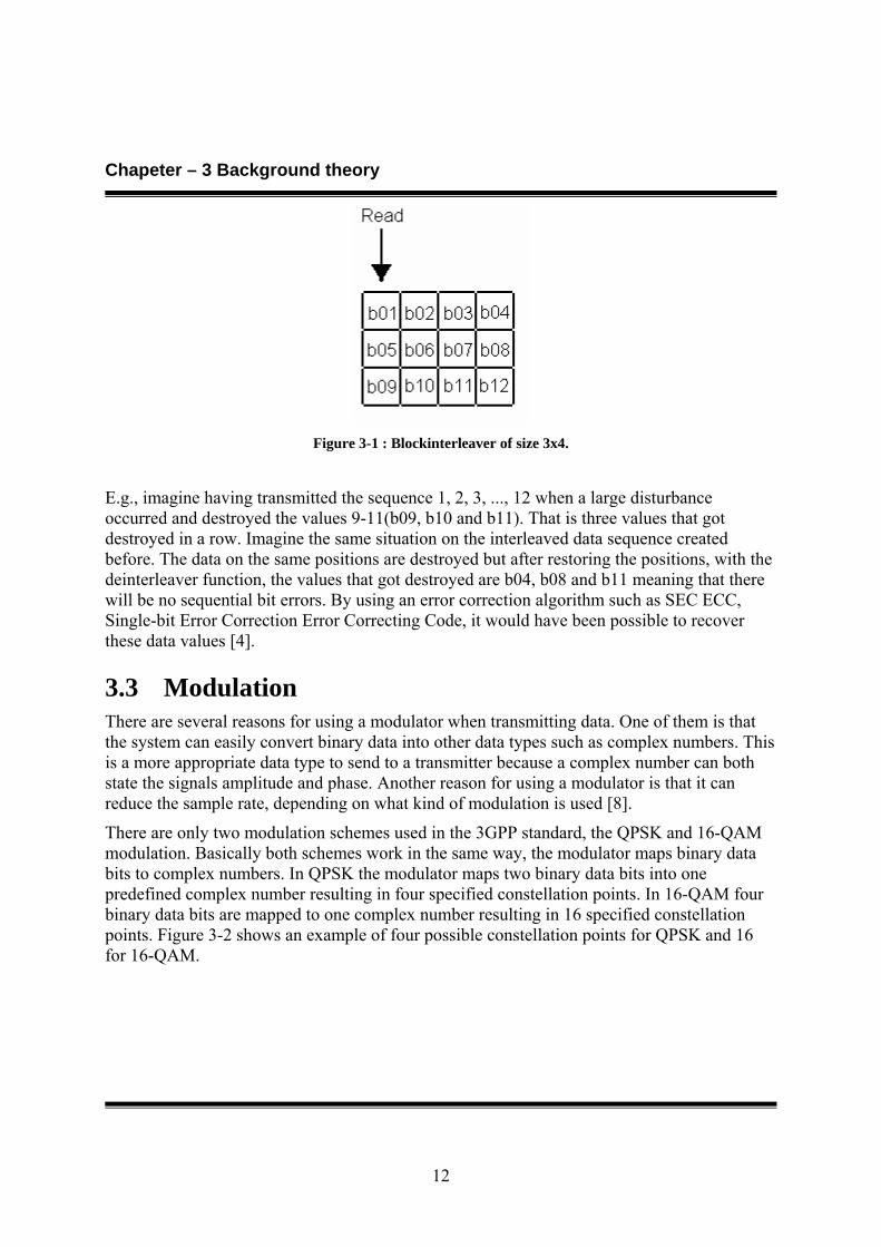
The basic idea of a blockinterleaver is to write data in rows. When the block is filled the data is read from columns. Figure 3-1 illustrates the case when 12 data symbols are interleaved.
Chapeter – 3 Background theory
12
Figure 3-1 : Blockinterleaver of size 3x4.
E.g., imagine having transmitted the sequence 1, 2, 3, ..., 12 when a large disturbance occurred and destroyed the values 9-11(b09, b10 and b11). That is three values that got destroyed in a row. Imagine the same situation on the interleaved data sequence created before. The data on the same positions are destroyed but after restoring the positions, with the deinterleaver function, the values that got destroyed are b04, b08 and b11 meaning that there will be no sequential bit errors. By using an error correction algorithm such as SEC ECC, Single-bit Error Correction Error Correcting Code, it would have been possible to recover these data values [4].
3.3 Modulation There are several reasons for using a modulator when transmitting data. One of them is that the system can easily convert binary data into other data types such as complex numbers. This is a more appropriate data type to send to a transmitter because a complex number can both state the signals amplitude and phase. Another reason for using a modulator is that it can reduce the sample rate, depending on what kind of modulation is used [8].
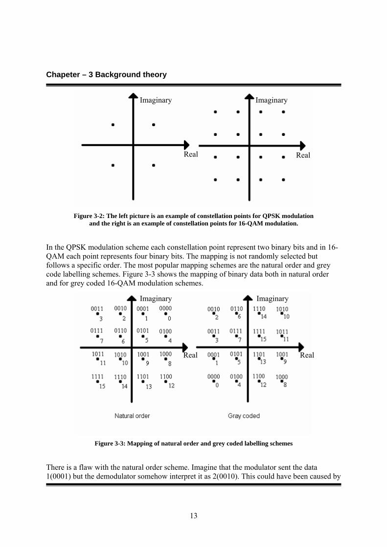
There are only two modulation schemes used in the 3GPP standard, the QPSK and 16-QAM modulation. Basically both schemes work in the same way, the modulator maps binary data bits to complex numbers. In QPSK the modulator maps two binary data bits into one predefined complex number resulting in four specified constellation points. In 16-QAM four binary data bits are mapped to one complex number resulting in 16 specified constellation points. Figure 3-2 shows an example of four possible constellation points for QPSK and 16 for 16-QAM.
Chapeter – 3 Background theory
13
Figure 3-2: The left picture is an example of constellation points for QPSK modulation
and the right is an example of constellation points for 16-QAM modulation.
In the QPSK modulation scheme each constellation point represent two binary bits and in 16-QAM each point represents four binary bits. The mapping is not randomly selected but follows a specific order. The most popular mapping schemes are the natural order and grey code labelling schemes. Figure 3-3 shows the mapping of binary data both in natural order and for grey coded 16-QAM modulation schemes.
Figure 3-3: Mapping of natural order and grey coded labelling schemes
There is a flaw with the natural order scheme. Imagine that the modulator sent the data 1(0001) but the demodulator somehow interpret it as 2(0010). This could have been caused by
Real Real
Imaginary Imaginary
Real Real
Imaginary Imaginary

Chapeter – 3 Background theory
14
various reasons such as noise, multipaths or many others. The result of this small mistake will result in two bit errors.
Gray code scheme eliminates this kind of two bit errors between two neighbouring points. Using the same coordinates as the previous scheme the Gray code scheme would send 14(1110) and interpret 6(0110) instead. The same error as before but now it will only result in 1 bit error instead. Figure 3-4 has markings on the bits where error has occurred [8].
Figure 3-4: 16-QAM modulation errors with different schemes
3.4 Spreading In a CDMA system different users are separated by assigning each user an individual spreading code. Every individual spreading code is orthogonal against all other spreading codes used by the system. Therefore multiple users can transmit data at the same time and at the same frequency without interfering with each other, [15].
This section illustrates spreading with 4-elements long complex spreading codes to illustrate how spreading is preformed.
3.4.1 Advantages of using spreading This section explains the advantages of using spreading.
Real Real
Imaginary Imaginary

Chapeter – 3 Background theory
15
Multiple access If multiple users transmit different signals in the same time/frequency the receiver can still distinguish between the different signals, provided that each signal has been coded with a unique code that has very low correlation17 with the codes used by other users, [15].
Protection against multipath interference Interference caused by multipaths can be reduced. This can be done in different ways but we have chosen to implement a rake18 function to counter the effects of multipaths, see section 3.9.
Privacy The signal can only be despread, detected, if the user has the correct code, [15].
Interference rejection By cross-correlating the received signal with the spreading code used for spreading the signal the spread data will be despread. Narrowband interference will instead be spread making it appear as background noise. Figure 3-5 shows an illustration of this. P is the energy and f is the frequency, [15].
Figure 3-5: The despreading operations effect on signals and interference
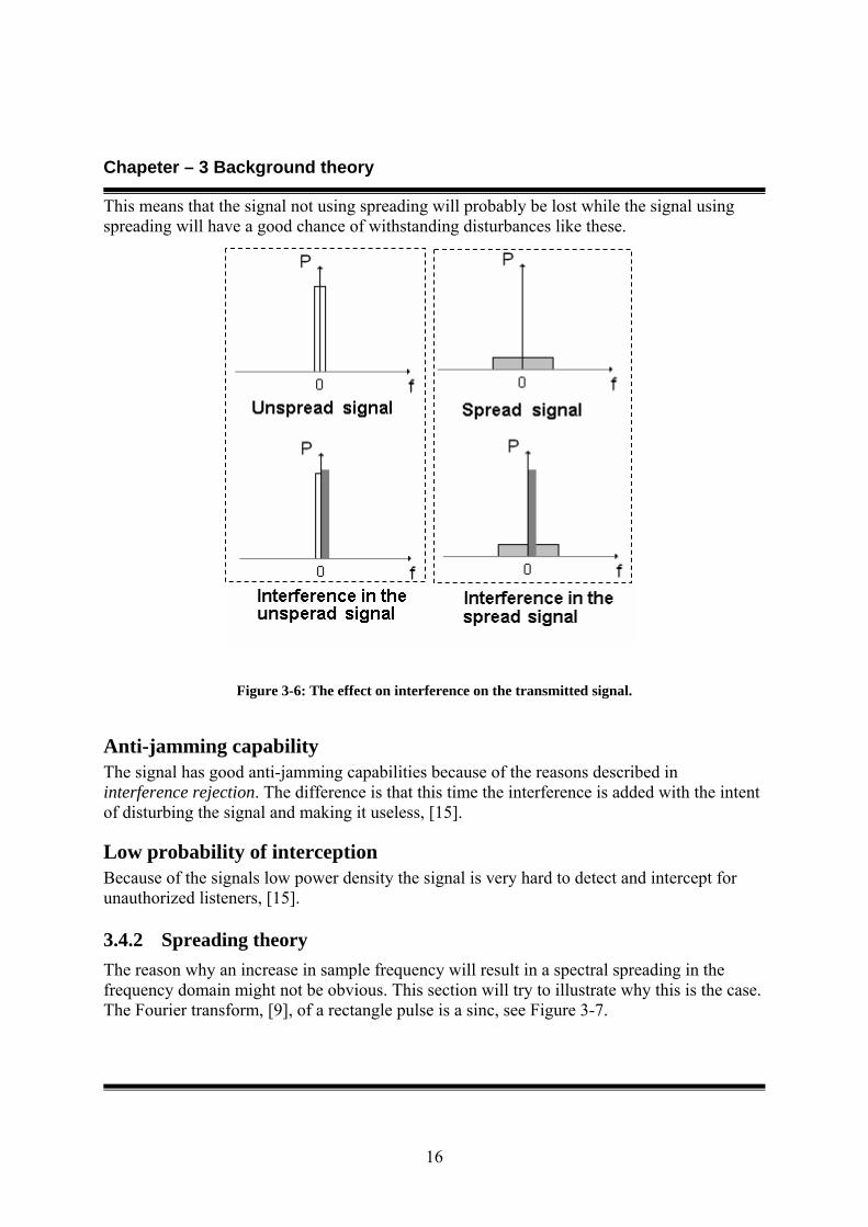
The signal is also be more tolerable against interference in other ways. Figure 3-6 illustrate the case when a narrowband signal gets destroyed by a strong narrowband disturbances, but the same disturbance in a system using spreading will only loose a small part of the signal.
17 Correlation – Correlation is a time-domain function that is a measure of how much a signal shape, or waveform, resembles a predefined pattern. 18 Rake – An algorithm that is used to strengthen the received signal
Chapeter – 3 Background theory
16
This means that the signal not using spreading will probably be lost while the signal using spreading will have a good chance of withstanding disturbances like these.
Figure 3-6: The effect on interference on the transmitted signal.
Anti-jamming capability The signal has good anti-jamming capabilities because of the reasons described in interference rejection. The difference is that this time the interference is added with the intent of disturbing the signal and making it useless, [15].
Low probability of interception Because of the signals low power density the signal is very hard to detect and intercept for unauthorized listeners, [15].
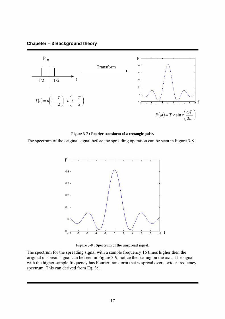
3.4.2 Spreading theory The reason why an increase in sample frequency will result in a spectral spreading in the frequency domain might not be obvious. This section will try to illustrate why this is the case. The Fourier transform, [9], of a rectangle pulse is a sinc, see Figure 3-7.
Chapeter – 3 Background theory
17
Figure 3-7 : Fourier transform of a rectangle pulse.
The spectrum of the original signal before the spreading operation can be seen in Figure 3-8.
Figure 3-8 : Spectrum of the unspread signal.
The spectrum for the spreading signal with a sample frequency 16 times higher then the original unspread signal can be seen in Figure 3-9, notice the scaling on the axis. The signal with the higher sample frequency has Fourier transform that is spread over a wider frequency spectrum. This can derived from Eq. 3:1.
-T/2 T/2 t
Transform
( ) ⎟
⎠⎞
⎜⎝⎛ −−⎟
⎠⎞
⎜⎝⎛ +=
22TtuTtutf
( ) ⎟⎠⎞
⎜⎝⎛×=
πωω2
sin TcTF
P P
f
f
P
Chapeter – 3 Background theory
18
Eq. 3:1 ( ) ⎟⎠⎞
⎜⎝⎛×=
πωω2
sin TcTF
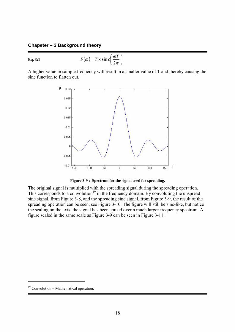
A higher value in sample frequency will result in a smaller value of T and thereby causing the sinc function to flatten out.
Figure 3-9 : Spectrum for the signal used for spreading.
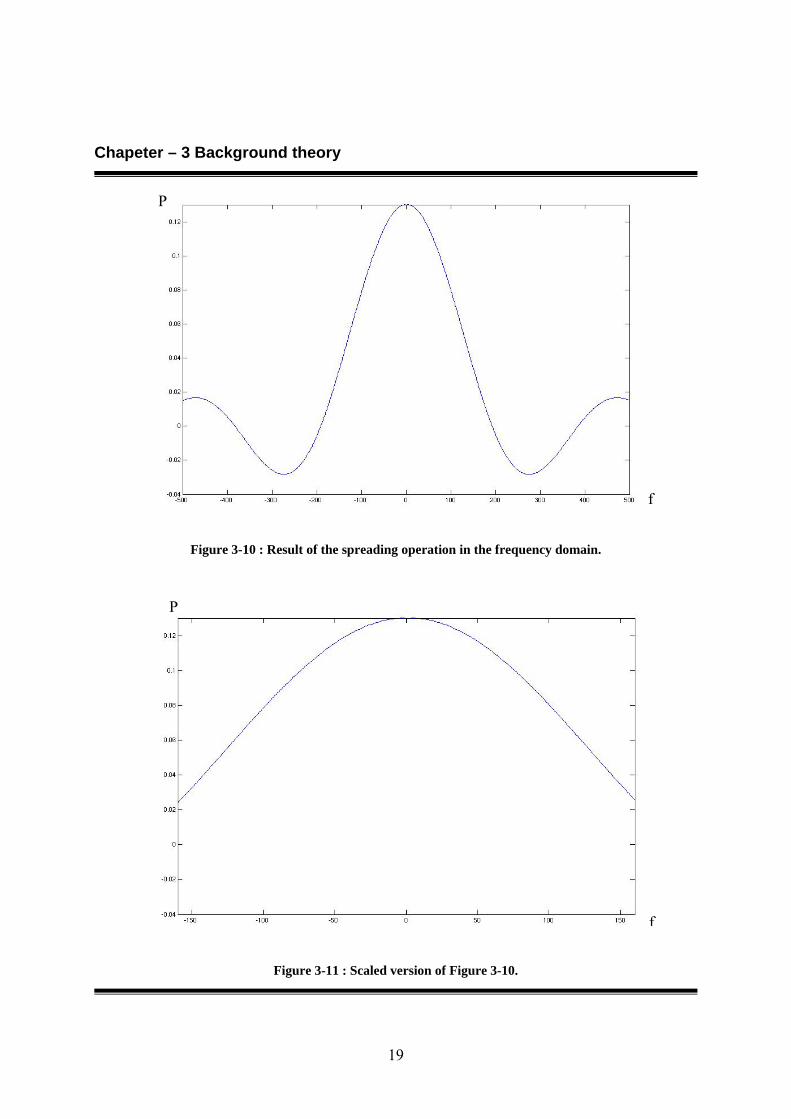
The original signal is multiplied with the spreading signal during the spreading operation. This corresponds to a convolution19 in the frequency domain. By convoluting the unspread sinc signal, from Figure 3-8, and the spreading sinc signal, from Figure 3-9, the result of the spreading operation can be seen, see Figure 3-10. The figure will still be sinc-like, but notice the scaling on the axis, the signal has been spread over a much larger frequency spectrum. A figure scaled in the same scale as Figure 3-9 can be seen in Figure 3-11.
19 Convolution – Mathematical operation.
f
P
Chapeter – 3 Background theory
19
Figure 3-10 : Result of the spreading operation in the frequency domain.
Figure 3-11 : Scaled version of Figure 3-10.
f
f
P
P
Chapeter – 3 Background theory
20
3.4.3 Spreading codes What we will refer to as a spreading code in this document consists of two parts. One channelisation code, which consists of an OVSF20 code, and one scrambling sequence21. The channelisation code allows for multiple accesses since they are orthogonal. The scrambling sequence makes the signal more effective in a multipath environment by reducing the autocorrelation22 between the codes. It is also used to distinguish between signals transmitted in different cells, [11].
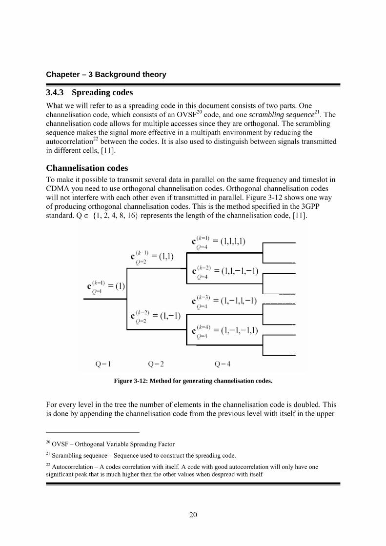
Channelisation codes To make it possible to transmit several data in parallel on the same frequency and timeslot in CDMA you need to use orthogonal channelisation codes. Orthogonal channelisation codes will not interfere with each other even if transmitted in parallel. Figure 3-12 shows one way of producing orthogonal channelisation codes. This is the method specified in the 3GPP standard. Q ∈ {1, 2, 4, 8, 16} represents the length of the channelisation code, [11].
Figure 3-12: Method for generating channelisation codes.
For every level in the tree the number of elements in the channelisation code is doubled. This is done by appending the channelisation code from the previous level with itself in the upper
20 OVSF – Orthogonal Variable Spreading Factor 21 Scrambling sequence – Sequence used to construct the spreading code. 22 Autocorrelation – A codes correlation with itself. A code with good autocorrelation will only have one significant peak that is much higher then the other values when despread with itself
Chapeter – 3 Background theory
21
branch and –itself in the lower branch. As can be seen in Figure 3-12 ( )11
11
12 , =
===
== = k
QkQ
kQ ccc
and ( )11
11
22 , =
===
== −= k
QkQ
kQ ccc .
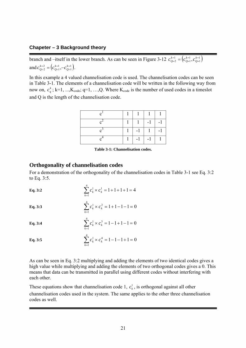
In this example a 4 valued channelisation code is used. The channelisation codes can be seen in Table 3-1. The elements of a channelisation code will be written in the following way from now on, k
qc ; k=1, ...,Kcode; q=1, …,Q. Where Kcode is the number of used codes in a timeslot and Q is the length of the channelisation code.
c1 1 1 1 1
c2 1 1 -1 -1
c3 1 -1 1 -1
c4 1 -1 -1 1
Table 3-1: Channelisation codes.
Orthogonality of channelisation codes For a demonstration of the orthogonality of the channelisation codes in Table 3-1 see Eq. 3:2 to Eq. 3:5.
Eq. 3:2 ∑=
=+++=×4
1
11 41111k
kk cc
Eq. 3:3 ∑=
=−−+=×4
1
21 01111k
kk cc
Eq. 3:4 ∑=
=−+−=×4
1
31 01111k
kk cc
Eq. 3:5 ∑=
=+−−=×4
1
41 01111k
kk cc
As can be seen in Eq. 3:2 multiplying and adding the elements of two identical codes gives a high value while multiplying and adding the elements of two orthogonal codes gives a 0. This means that data can be transmitted in parallel using different codes without interfering with each other.
These equations show that channelisation code 1, 1kc , is orthogonal against all other
channelisation codes used in the system. The same applies to the other three channelisation codes as well.
Chapeter – 3 Background theory
22
Scrambling sequence The second part of the spreading operation is an element-wise multiplication of the OVSF coded data with a scrambling sequence. The scrambling sequence helps with multipath detection since it reduces the autocorrelation of time-delayed versions of the signal. The scrambling sequence also separates users in different cells from each other, [11].
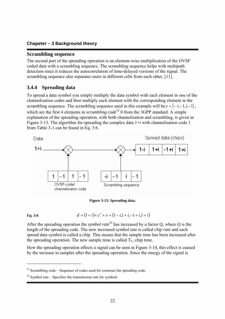
3.4.4 Spreading data To spread a data symbol you simply multiply the data symbol with each element in one of the channelisation codes and then multiply each element with the corresponding element in the scrambling sequence. The scrambling sequence used in this example will be { }1,,1, −−−= iiv , which are the first 4 elements in scrambling code23 0 from the 3GPP standard. A simple explanation of the spreading operation, with both channelisation and scrambling, is given in Figure 3-13. The algorithm for spreading the complex data 1+i with channelisation code 1 from Table 3-1 can be found in Eq. 3:6.
Figure 3-13: Spreading data.
Eq. 3:6 ( ) ( )iiiivcid ++−+−=××+= 1,1,1,11 1
After the spreading operation the symbol rate24 has increased by a factor Q, where Q is the length of the spreading code. The new increased symbol rate is called chip rate and each spread data symbol is called a chip. This means that the sample time has been increased after the spreading operation. The new sample time is called TC, chip time.
How the spreading operation effects a signal can be seen in Figure 3-14, this effect is caused by the increase in samples after the spreading operation. Since the energy of the signal is
23 Scrambling code – Sequence of codes used for construct the spreading code. 24 Symbol rate – Specifies the transmission rate for symbols
Chapeter – 3 Background theory
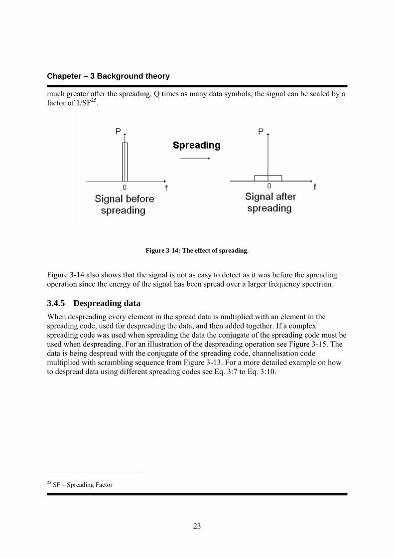
23
much greater after the spreading, Q times as many data symbols, the signal can be scaled by a factor of 1/SF25.
Figure 3-14: The effect of spreading.
Figure 3-14 also shows that the signal is not as easy to detect as it was before the spreading operation since the energy of the signal has been spread over a larger frequency spectrum.
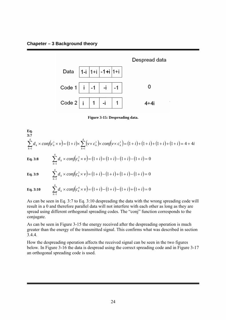
3.4.5 Despreading data When despreading every element in the spread data is multiplied with an element in the spreading code, used for despreading the data, and then added together. If a complex spreading code was used when spreading the data the conjugate of the spreading code must be used when despreading. For an illustration of the despreading operation see Figure 3-15. The data is being despread with the conjugate of the spreading code, channelisation code multiplied with scrambling sequence from Figure 3-13. For a more detailed example on how to despread data using different spreading codes see Eq. 3:7 to Eq. 3:10.
25 SF – Spreading Factor
Chapeter – 3 Background theory
24
Figure 3-15: Despreading data.
Eq. 3:7
( ) ( ) ( ) ( ) ( ) ( ) ( ) ( )∑ ∑= =
+=+++++++=××××+=××4
1
4
1
111 4411111k k
kkkk iiiiicvconjcvivcconjd
Eq. 3:8 ( ) ( ) ( ) ( ) ( )∑=
=+−+−+++=××4
1
2 01111k
kk iiiivcconjd
Eq. 3:9 ( ) ( ) ( ) ( ) ( )∑=
=+−+++−+=××4
1
3 01111k
kk iiiivcconjd
Eq. 3:10 ( ) ( ) ( ) ( ) ( )∑=
=+++−+−+=××4
1
4 01111k
kk iiiivcconjd
As can be seen in Eq. 3:7 to Eq. 3:10 despreading the data with the wrong spreading code will result in a 0 and therefore parallel data will not interfere with each other as long as they are spread using different orthogonal spreading codes. The “conj” function corresponds to the conjugate.
As can be seen in Figure 3-15 the energy received after the despreading operation is much greater than the energy of the transmitted signal. This confirms what was described in section 3.4.4.
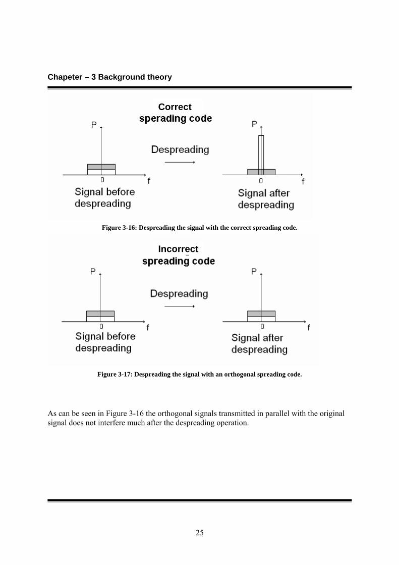
How the despreading operation affects the received signal can be seen in the two figures below. In Figure 3-16 the data is despread using the correct spreading code and in Figure 3-17 an orthogonal spreading code is used.
Chapeter – 3 Background theory
25
Figure 3-16: Despreading the signal with the correct spreading code.
Figure 3-17: Despreading the signal with an orthogonal spreading code.
As can be seen in Figure 3-16 the orthogonal signals transmitted in parallel with the original signal does not interfere much after the despreading operation.
Correct
Incorrect
Chapeter – 3 Background theory
26
3.5 Frames and Timeslots structure In the 3GPP standard data is transmitted in timeslots which are a part of a bigger structure called frames. The timeslots are divided into three different blocks; data; midamble and a guard period26. This section describes the midamble, the structure of frames and timeslots in both 3.84Mcp and 1.28Mcp. All structures explained here are for TDD transmission, [10].
3.5.1 Midamble The midamble is used to synchronize the system and test the dispreading parameters calculated in the receiver. The midamble consists of training sequences, known sequences of codes that are used for testing the reliability of the despread received data. These sequences are either identical or shifted versions of the same basic midamble code27. The shift in the midamble is detected by correlation with the midamble code used in the current cell. The length of the midamble code can be either 256 or 512 chips depending on which burst type28 that is being used. The longer the midamble code is the more training sequences can be supported, [10].
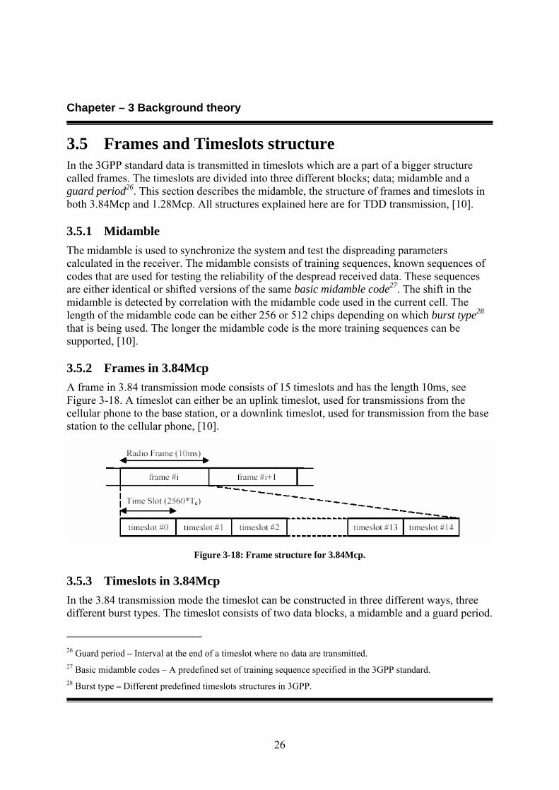
3.5.2 Frames in 3.84Mcp A frame in 3.84 transmission mode consists of 15 timeslots and has the length 10ms, see Figure 3-18. A timeslot can either be an uplink timeslot, used for transmissions from the cellular phone to the base station, or a downlink timeslot, used for transmission from the base station to the cellular phone, [10].
Figure 3-18: Frame structure for 3.84Mcp.
3.5.3 Timeslots in 3.84Mcp In the 3.84 transmission mode the timeslot can be constructed in three different ways, three different burst types. The timeslot consists of two data blocks, a midamble and a guard period.
26 Guard period – Interval at the end of a timeslot where no data are transmitted. 27 Basic midamble codes – A predefined set of training sequence specified in the 3GPP standard. 28 Burst type – Different predefined timeslots structures in 3GPP.
Chapeter – 3 Background theory
27
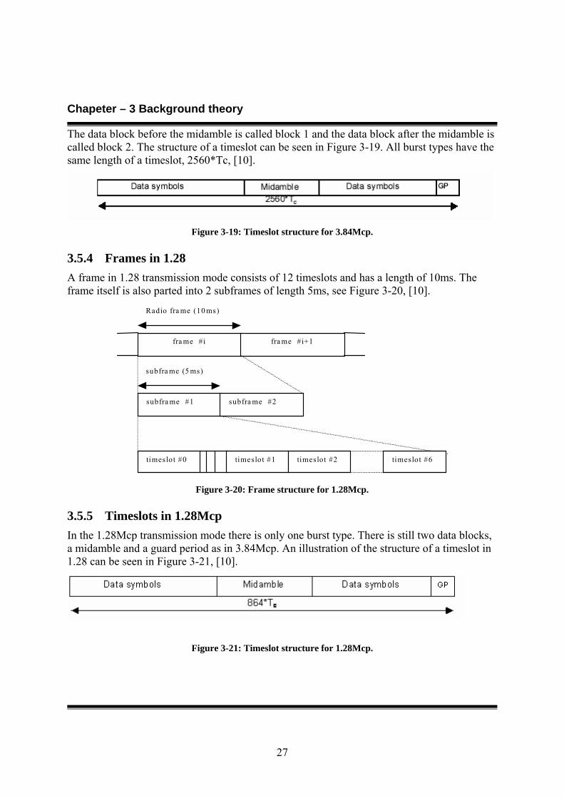
The data block before the midamble is called block 1 and the data block after the midamble is called block 2. The structure of a timeslot can be seen in Figure 3-19. All burst types have the same length of a timeslot, 2560*Tc, [10].
Figure 3-19: Timeslot structure for 3.84Mcp.
3.5.4 Frames in 1.28 A frame in 1.28 transmission mode consists of 12 timeslots and has a length of 10ms. The frame itself is also parted into 2 subframes of length 5ms, see Figure 3-20, [10].
fra me #i fra me #i+1
Radio fra me (10 ms)
subfra me #1 subfra me #2
subfra me (5 ms)
timeslot #0 timeslot #1 timeslot #2 timeslot #6
Figure 3-20: Frame structure for 1.28Mcp.
3.5.5 Timeslots in 1.28Mcp In the 1.28Mcp transmission mode there is only one burst type. There is still two data blocks, a midamble and a guard period as in 3.84Mcp. An illustration of the structure of a timeslot in 1.28 can be seen in Figure 3-21, [10].
Figure 3-21: Timeslot structure for 1.28Mcp.

Chapeter – 3 Background theory
28
3.6 Synchronisation codes for 3.84Mcp This section describes the synchronisation codes, which consist of one PSC and three secondary SCH codes. The first one to be described is the PSC, which is used for packet detection. The three secondary SCH codes, which transmit cell specific information, are transmitted in parallel with the PSC which means that if the system finds the PSC it also finds the secondary SCH codes. More in detail about secondary SCH codes can be found in section 3.6.2. These both synchronisation codes are used in the TDD standard where the data rate is 3.84 Mcps and they are sent in parallel with each other. These codes are located in either the first or the ninth timeslot of the frame.
Figure 3-22 illustrates an example of placement of synchronisations codes where cj,i are secondary SCH codes, bi are factors to make the secondary SCH codes complex, PP is the power level of the PSC, PS is the power level of the three secondary SCH codes, Cp is the PSC and tOffset is offset of where the synchronisation codes are located [10].
Figure 3-22: Placement of synchronisation codes.
tOffset,n
Cp
b1Cj,1
b2Cj,2
b3Cj,3
PP
PS
PS/3
PS/3
PS/3
Chapeter – 3 Background theory
29
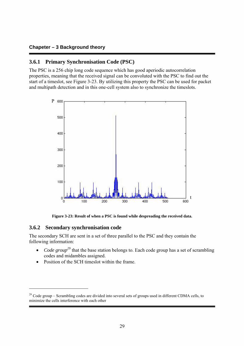
3.6.1 Primary Synchronisation Code (PSC) The PSC is a 256 chip long code sequence which has good aperiodic autocorrelation properties, meaning that the received signal can be convoluted with the PSC to find out the start of a timeslot, see Figure 3-23. By utilizing this property the PSC can be used for packet and multipath detection and in this one-cell system also to synchronize the timeslots.
Figure 3-23: Result of when a PSC is found while despreading the received data.
3.6.2 Secondary synchronisation code The secondary SCH are sent in a set of three parallel to the PSC and they contain the following information:
• Code group29 that the base station belongs to. Each code group has a set of scrambling codes and midambles assigned.
• Position of the SCH timeslot within the frame.
29 Code group – Scrambling codes are divided into several sets of groups used in different CDMA cells, to minimize the cells interference with each other
t
P
Chapeter – 3 Background theory
30
From the first point information point the system can distinguish which scramble codes are used and also the time offset, tOffset, which informs the system of where the synchronisation codes are located in the timeslot, see Figure 3-22.
The tOffset is one of the 32 values calculate by the transmitter with the Eq. 3:11:
Eq. 3:11 ( ) 31....,,0;16487201648
, =⎩⎨⎧
≥⋅+<⋅⋅
= nnTnnTn
tc
cnoffset
There are two timeslots within a frame where the synchronisation codes can be located and 32 different ways to place the synchronisations codes within a timeslot. Therefore the SCH can be at 2x32 different places in a frame. The reason for having the tOffset is to separate different cells so that their interference on each other are minimized.
From the second point the system can derive in which timeslot the SCH is located (first or ninth) in the frame [12].
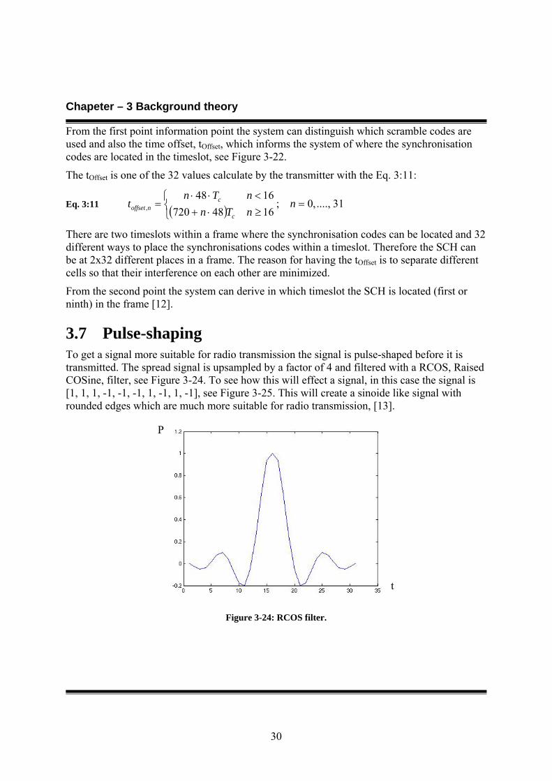
3.7 Pulse-shaping To get a signal more suitable for radio transmission the signal is pulse-shaped before it is transmitted. The spread signal is upsampled by a factor of 4 and filtered with a RCOS, Raised COSine, filter, see Figure 3-24. To see how this will effect a signal, in this case the signal is [1, 1, 1, -1, -1, -1, 1, -1, 1, -1], see Figure 3-25. This will create a sinoide like signal with rounded edges which are much more suitable for radio transmission, [13].
Figure 3-24: RCOS filter.
P
t

Chapeter – 3 Background theory
31
Figure 3-25: The effect of filtering the signal with a RCOS filter.
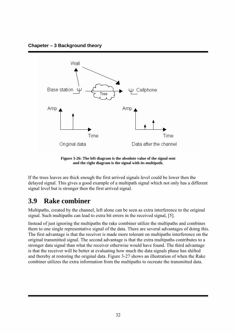
3.8 Multipaths Multipaths are created when the same signals arrives to a receiver multiple times. The different times of arrival are caused when the signal bounces on obstacles, e.g. buildings, cars, mountains etc. These signals are usually not just delayed, most of the times the signals phases are also shifted caused by the reflecting object. Another possible difference between them is that the signals could have different signal levels, which depend on the route the signal has travelled before it reaches the receiver.
E.g. consider the case where there is one signal that arrives twice to a receiver, the first arrived signal went straight from the transmitter to the receiver passing through trees and the second one took a detour by first bouncing of a wall of a building further away before it arrives. An illustration of this can be seen in Figure 3-26.
Original signal Filtered signal
P
t
Chapeter – 3 Background theory
32
Figure 3-26: The left diagram is the absolute value of the signal sent
and the right diagram is the signal with its multipath.
If the trees leaves are thick enough the first arrived signals level could be lower then the delayed signal. This gives a good example of a multipath signal which not only has a different signal level but is stronger then the first arrived signal.
3.9 Rake combiner Multipaths, created by the channel, left alone can be seen as extra interference to the original signal. Such multipaths can lead to extra bit errors in the received signal, [5].
Instead of just ignoring the multipaths the rake combiner utilize the multipaths and combines them to one single representative signal of the data. There are several advantages of doing this. The first advantage is that the receiver is made more tolerant on multipaths interference on the original transmitted signal. The second advantage is that the extra multipaths contributes to a stronger data signal than what the receiver otherwise would have found. The third advantage is that the receiver will be better at evaluating how much the data signals phase has shifted and thereby at restoring the original data. Figure 3-27 shows an illustration of when the Rake combiner utilizes the extra information from the multipaths to recreate the transmitted data.

Chapeter – 3 Background theory
33
Figure 3-27: The energy of the data signal, path from transmission via the channel to after the rake
combiner.
It is impossible for the rake combiner to utilize all multipath signals because there are not any limitations on how many multipaths an environment can create. The rake combiner will therefore only select a few, out of the found multipaths, and combine these to restore the data signal. The number of paths to be included is set by the number of fingers the rake will use. If the rake combiner uses one rake finger it will only use the strongest signal found. Using two rake fingers it will use the two strongest signals found and so on.
Chapeter – 4 System overview
34
4 System overview
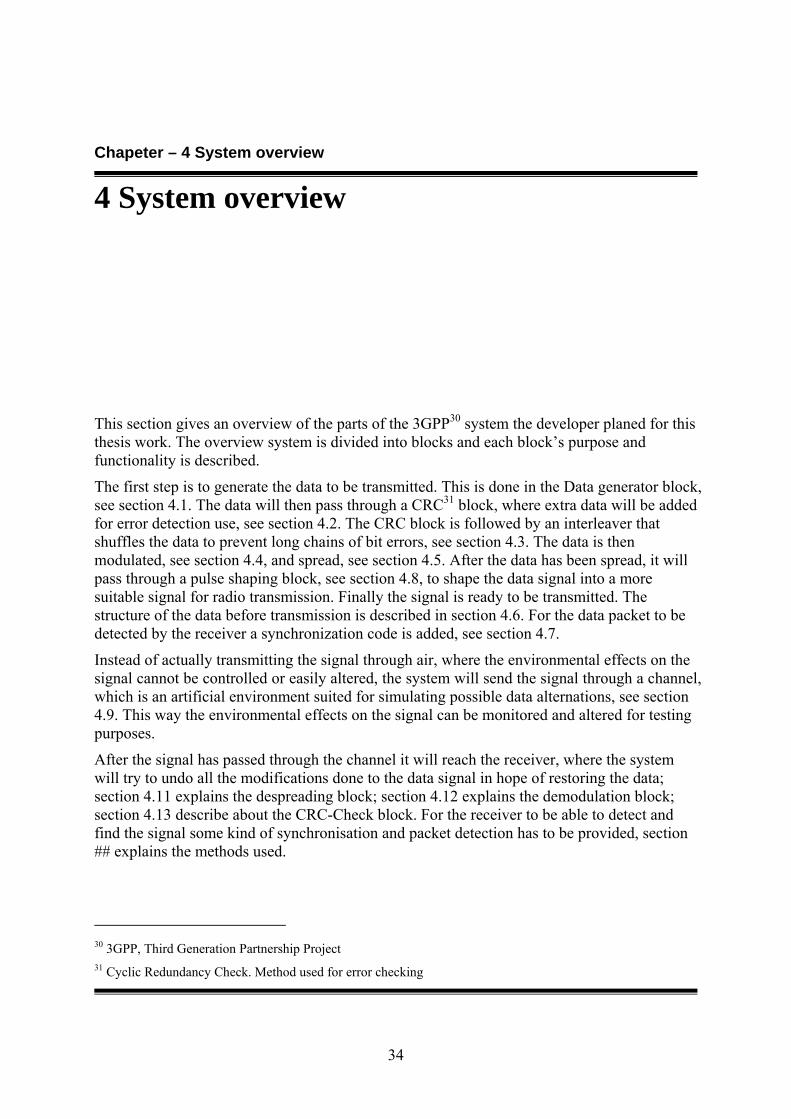
This section gives an overview of the parts of the 3GPP30 system the developer planed for this thesis work. The overview system is divided into blocks and each block’s purpose and functionality is described.
The first step is to generate the data to be transmitted. This is done in the Data generator block, see section 4.1. The data will then pass through a CRC31 block, where extra data will be added for error detection use, see section 4.2. The CRC block is followed by an interleaver that shuffles the data to prevent long chains of bit errors, see section 4.3. The data is then modulated, see section 4.4, and spread, see section 4.5. After the data has been spread, it will pass through a pulse shaping block, see section 4.8, to shape the data signal into a more suitable signal for radio transmission. Finally the signal is ready to be transmitted. The structure of the data before transmission is described in section 4.6. For the data packet to be detected by the receiver a synchronization code is added, see section 4.7.
Instead of actually transmitting the signal through air, where the environmental effects on the signal cannot be controlled or easily altered, the system will send the signal through a channel, which is an artificial environment suited for simulating possible data alternations, see section 4.9. This way the environmental effects on the signal can be monitored and altered for testing purposes.
After the signal has passed through the channel it will reach the receiver, where the system will try to undo all the modifications done to the data signal in hope of restoring the data; section 4.11 explains the despreading block; section 4.12 explains the demodulation block; section 4.13 describe about the CRC-Check block. For the receiver to be able to detect and find the signal some kind of synchronisation and packet detection has to be provided, section ## explains the methods used.
30 3GPP, Third Generation Partnership Project 31 Cyclic Redundancy Check. Method used for error checking

Chapeter – 4 System overview
35
To examine the robustness of the system SNR32 and BER33, see section 4.14 respectively 4.15, will be calculated for each transmission of a signal. Figure 4-1 show a block diagram over the system.
Figure 4-1: System structure.
32 SNR, Signal to Noise Ratio, relation between the sent data and the disturbance noise power level. 33 BER, Bit Error Rate, calculation of number of bit errors on the received data.
Transmitter
Receiver
Interleaver CRC Data generator
Modulation
Spreading
Creating slots
Sync. Code
Channel
Detection & sync
Rake-combiner
Depreading
Demodulation
SNR & BER
CRC-Check Deinterleaver
Pulse shaping
Chapeter – 4 System overview
36
4.1 Data generator The data generator is a randomizer used to generate a random sequence of data for transmission. The data generated is a binary sequence where “1” represents binary 1 and “-1” represents 0. The reason for mapping 0 to -1 is because the radio antenna has trouble sending/receiving 0 otherwise.
4.2 CRC No support for CRC is implemented. The implementation would have been time consuming and other functionalities were prioritized because it was an optional requirement.
4.3 Interleaver No support for interleaving is implemented. The implementation would have been time consuming and other functionalities were prioritized because it was an optional requirement.
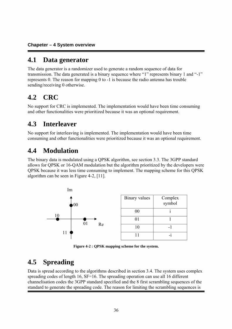
4.4 Modulation The binary data is modulated using a QPSK algorithm, see section 3.3. The 3GPP standard allows for QPSK or 16-QAM modulation but the algorithm prioritized by the developers were QPSK because it was less time consuming to implement. The mapping scheme for this QPSK algorithm can be seen in Figure 4-2, [11].
Figure 4-2 : QPSK mapping scheme for the system.
4.5 Spreading Data is spread according to the algorithms described in section 3.4. The system uses complex spreading codes of length 16, SF=16. The spreading operation can use all 16 different channelisation codes the 3GPP standard specified and the 8 first scrambling sequences of the standard to generate the spreading code. The reason for limiting the scrambling sequences is
10
11
01
00
Im
Re
Binary values Complex symbol
00 i
01 1
10 -1
11 -i

Chapeter – 4 System overview
37
because the developers find no gain by implementing all 128 sequences when there simulating only include one base station and one cellular phone. By implementing at least eight of the scrambling sequence the system can have some options available for generating the spreading code.
4.6 Creating slots Before the data can be transmitted it needs to be structured according to the 3GPP standard. The data to be transmitted is structured into timeslots.
4.6.1 Timeslots 3.84Mcp The burst type implemented in the system is burst type 3. The burst type was chosen because it has a longer guard period which makes it more robust against disturbances from multipaths, see Figure 4-1. The down side of this burst type compared with the others is it has longer midamble code length, 512 chips instead of 256 chips, this means the package will have lesser room for data symbols to be transmitted, [10].
Figure 4-1: Timeslot structure for 3.84Mcp.
4.6.2 Timeslots 1.28Mcp In the 1.28Mcp transmission mode there is only one burst type specified in the 3GPP standard. Therefore this is used in the system, see Figure 4-2, [10].
Data symbols352 chips
Midamble144 chips
Data symbols352 chips
GP16CP
864*Tc
Figure 4-2: Timeslot structure for 1.28Mcp.
4.6.3 Midamble Two midamble codes are implemented in the system, one for 3.84Mcp and one for 1.28Mcp. The midamble code is generated according to the 3GPP standard and is used to create the desired timeslot structure. The receiver does not use the midamble since the system only consist of one cell and all the synchronization needed can be performed with the PSC, [10].
Chapeter – 4 System overview
38
4.7 Synchronisation codes for 3.84Mcp Every other timeslot the transmitter transmits synchronisation codes instead of a data signal. These codes consist of one PSC and three secondary SCH codes. All four of these codes are transmitted in parallel, section 3.6. The synchronisation codes are used by the receiver to synchronize the reception of timeslots.
To be as practical as possible we generated the synchronisation codes first in Matlab then we copied them into arrays in C++.
The PSC, Cp, we generated follows the 3GPP standard. The source for calculating the secondary SCH codes {C0, C1, C3, C4, C5, C6, C8, C10, C12, C13, C14, C15} are also from the standard, but because there are so many secondary SCH we decided to just implement the first three in the system, [11].
4.8 Pulse-shaping Before transmission the data signal is pulse shaped. This is done by upsampling the data signal, with a factor 4, and then filtering it with a RCOS filter. The upsampling is done by inserting three zeroes between the sample values in the data signal. The upsampling needs to be done in order to get a signal more suitable for radio transmission. Without the upsampling the sample values would be to close to each other and the filtering operation would not help much. The formula used when generating the RCOS filter, which can be seen in
Eq. 3:1 is specified in the 3GPP standard, [13]. chiprate
TC1
= and α=0.22 according to the
3GPP standard.
Eq. 4:1 ( )( ) ( )
⎟⎟
⎠
⎞
⎜⎜
⎝
⎛⎟⎟⎠
⎞⎜⎜⎝
⎛−
⎟⎟⎠
⎞⎜⎜⎝
⎛++⎟⎟
⎠
⎞⎜⎜⎝
⎛−
=20
41
1cos41sin
CC
CCC
Tt
Tt
Tt
Tt
Tt
tRC
απ
απααπ
4.9 Channel The purpose of the channels is to simulate a possible real life environment. This is done by altering the signals phase and amplitude and by adding multipaths and noise. The channel used in the system will achieve this by a Rayleigh fading channel that can add up to 5 paths to the original signal. Rayleigh fading is a phase interference fading caused by multipaths and can be approximated with Rayleigh distribution, [15]. The channel can also add random noise to the signal.
4.10 Rake combiner
Chapeter – 4 System overview
39
The rake combiner is an optional component for the system but using it in the receiver can prove advantageous. The rake combiner can be set up to use 1 to 6 rake fingers, usually more rake fingers results in fewer bit errors but more calculations are needed. The rake combiner is not specified in the 3GPP standard and therefore the algorithms used in the combiner have all been chosen by the developers.
The rake combiner is not a mandatory requirement for the system but the benefits from using are so great that a lot of time was spent on implementing it.
4.11 Despreading The purpose of the despreading operation is to undo the spreading done by the transmitter and thereby restore the modulated data. This is done by using the conjugate of the 16 symbol long spreading sequence used when spreading the data. The conjugate of the spreading code will be created by using the same functions that created the spreading code in the transmitter. How despreading works was explained in section 3.4.5.
4.12 Demodulation The purpose of the demodulator is to undo the modulation done by the modulator and restore the original binary data. The data is demodulated using the same QPSK modulating scheme used when modulating, see section 4.4.
4.13 CRC-Check Since no CRC is added in the transmitter no CRC-check is performed in the receiver.
4.14 Signal to Noise Ratio (SNR) The SNR is calculated to illustrate the relation between signal and noise. This is used when evaluating how interference will affect the system. A high SNR value means we have a strong signal compared to noise and a low SNR value means we have a weak signal compared to noise. The algorithm for calculating the SNR can be seen in Eq. 4:2, SE is the energy of the signal and NE is the energy of the noise.
The system calculates the mean value of the transmitted signal and the noise added and uses these values to get an approximation of the SNR in an entire timeslot. SNR calculations for different channel parameters are presented as a part of our test results in chapter 6 .
Eq. 4:2 E
E
NS
SNR log10×=
4.15 Bit Error Rate (BER)

Chapeter – 4 System overview
40
The BER is the relation between the number of bit errors and correctly received bits, having a high BER means there are a lot of bit errors and a low BER means there are few bit errors. The receiver calculates the BER to evaluate how well the data has been received. BER calculations are presented as a part of our test results in chapter 6 .
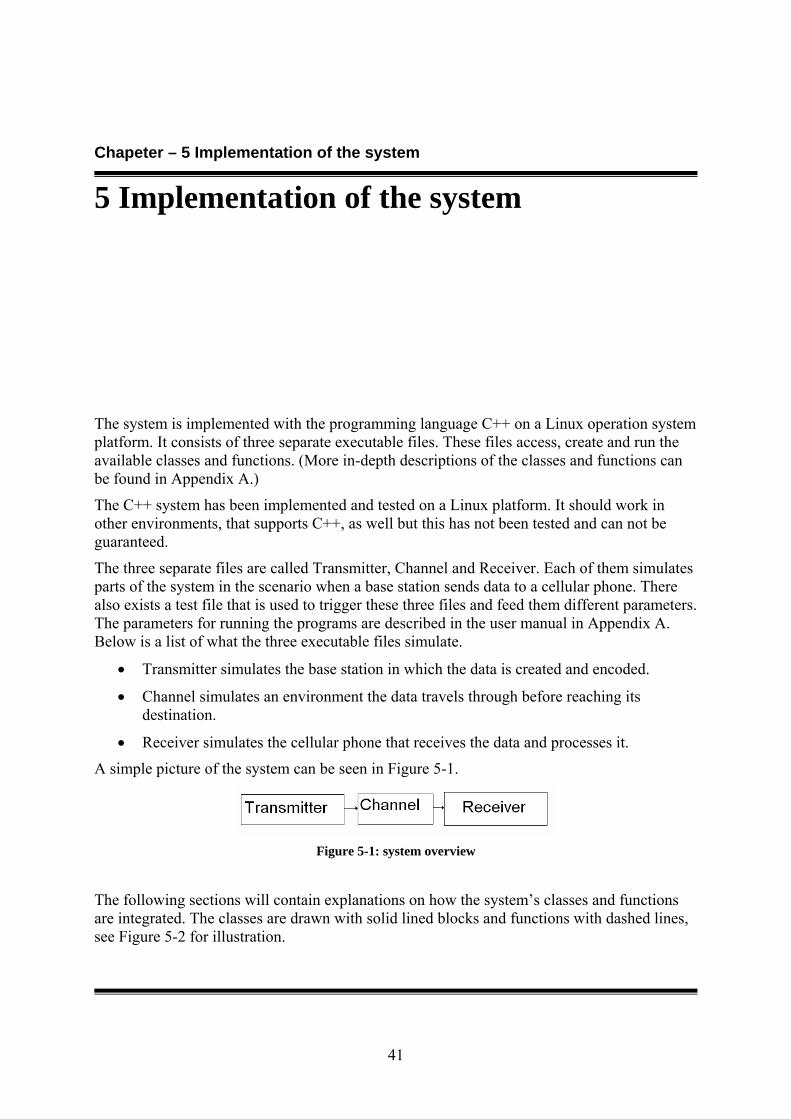
Chapeter – 5 Implementation of the system
41
5 Implementation of the system
The system is implemented with the programming language C++ on a Linux operation system platform. It consists of three separate executable files. These files access, create and run the available classes and functions. (More in-depth descriptions of the classes and functions can be found in Appendix A.)
The C++ system has been implemented and tested on a Linux platform. It should work in other environments, that supports C++, as well but this has not been tested and can not be guaranteed.
The three separate files are called Transmitter, Channel and Receiver. Each of them simulates parts of the system in the scenario when a base station sends data to a cellular phone. There also exists a test file that is used to trigger these three files and feed them different parameters. The parameters for running the programs are described in the user manual in Appendix A. Below is a list of what the three executable files simulate.
• Transmitter simulates the base station in which the data is created and encoded.
• Channel simulates an environment the data travels through before reaching its destination.
• Receiver simulates the cellular phone that receives the data and processes it.
A simple picture of the system can be seen in Figure 5-1.
Figure 5-1: system overview
The following sections will contain explanations on how the system’s classes and functions are integrated. The classes are drawn with solid lined blocks and functions with dashed lines, see Figure 5-2 for illustration.
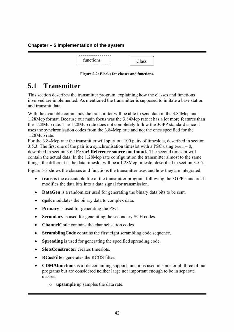
Chapeter – 5 Implementation of the system
42
Figure 5-2: Blocks for classes and functions.
5.1 Transmitter This section describes the transmitter program, explaining how the classes and functions involved are implemented. As mentioned the transmitter is supposed to imitate a base station and transmit data.
With the available commands the transmitter will be able to send data in the 3.84Mcp and 1.28Mcp format. Because our main focus was the 3.84Mcp rate it has a lot more features than the 1.28Mcp rate. The 1.28Mcp rate does not completely follow the 3GPP standard since it uses the synchronisation codes from the 3.84Mcp rate and not the ones specified for the 1.28Mcp rate. For the 3.84Mcp rate the transmitter will spurt out 100 pairs of timeslots, described in section 3.5.3. The first one of the pair is a synchronisation timeslot with a PSC using tOffset = 0, described in section 3.6.1Error! Reference source not found.. The second timeslot will contain the actual data. In the 1.28Mcp rate configuration the transmitter almost to the same things, the different is the data timeslot will be a 1.28Mcp timeslot described in section 3.5.5.
Figure 5-3 shows the classes and functions the transmitter uses and how they are integrated.
• trans is the executable file of the transmitter program, following the 3GPP standard. It modifies the data bits into a data signal for transmission.
• DataGen is a randomizer used for generating the binary data bits to be sent.
• qpsk modulates the binary data to complex data.
• Primary is used for generating the PSC.
• Secondary is used for generating the secondary SCH codes.
• ChannelCode contains the channelisation codes.
• ScramblingCode contains the first eight scrambling code sequence.
• Spreading is used for generating the specified spreading code.
• SlotsConstructor creates timeslots.
• RCosFilter generates the RCOS filter.
• CDMAfunctions is a file containing support functions used in some or all three of our programs but are considered neither large nor important enough to be in separate classes.
o upsample up samples the data rate.
functions Class
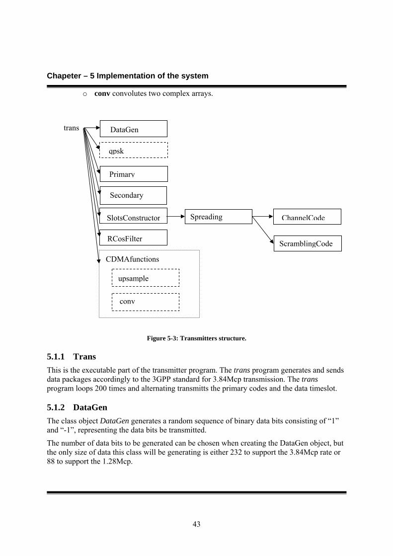
Chapeter – 5 Implementation of the system
43
o conv convolutes two complex arrays.
Figure 5-3: Transmitters structure.
5.1.1 Trans This is the executable part of the transmitter program. The trans program generates and sends data packages accordingly to the 3GPP standard for 3.84Mcp transmission. The trans program loops 200 times and alternating transmitts the primary codes and the data timeslot.
5.1.2 DataGen The class object DataGen generates a random sequence of binary data bits consisting of “1” and “-1”, representing the data bits be transmitted.
The number of data bits to be generated can be chosen when creating the DataGen object, but the only size of data this class will be generating is either 232 to support the 3.84Mcp rate or 88 to support the 1.28Mcp.
trans DataGen
qpsk
Secondary
upsample
SlotsConstructor
Primary
Spreading
RCosFilter
conv
ScramblingCode
CDMAfunctions
ChannelCode

Chapeter – 5 Implementation of the system
44
5.1.3 QPSK The modulation is done with the qpsk function. It takes in the binary data bits generated by DataGen and maps them to complex valued data symbols. The mapping scheme follows the one illustrated in Figure 4-2 in section 4.4.
5.1.4 Primary The primary class generates the 256 long primary synchronisation code, described in section 4.7. The PSC generation is done by repeating the sequence 'a' modulated by a Golay complementary sequence (REFERENS) and creating a complex-valued sequence with identical real and imaginary components.
a = <x1, x2, x3, ..., x16>=<1, 1, 1, 1, 1, 1, -1, -1, 1, -1, 1, -1, 1, -1, -1, 1>
The PSC is defined as Cp=<y(0), y(1), y(2), ..., y(255)> where y = (1+j) x <a, a, a, -a, -a, a, -a, -a, a, a, a, -a, a, -a ,a ,a >
the left most index corresponds to the chip transmitted first in time.
5.1.5 Secondary The secondary class generates the secondary synchronisation codes that are transmitted in parallell with the primary codes.
The 12 secondary SCH codes {C0, C1, C3, C4, C5, C6, C8, C10, C12, C13, C14, C15} are complex valued with identical real and imaginary components. They are constructed from the position wise multiplication of a Hadamard sequence and a sequence z, which is defined as:
z = <b, b, b,-b, b, b, -b, -b, b, -b, b, -b, -b, -b, -b, -b>
b = <x1, x2, x3, x4, x5, x6, x7, x8, -x9, -x10, -x11, -x12, -x13, -x14, -x15, -x16>
and x1, x2, x3, ..., x16 are the same as in definition of the sequence 'a' in the subsection before.
The Hadamard sequences are obtained as the rows in a matrix H8 constructed recursively by:
Eq. 5:1 1,
)1(
11
11
0
≥⎟⎟⎠
⎞⎜⎜⎝
⎛−
=
=
−−
−− kHH
HHH
H
kk
kkk
The rows are numbered from the top starting with row 0. Denote the n:th Hadamard sequence hn as a row of H8 numbered from the top, n = 0, 1, 2, …, 255, in the sequence. Furthermore let hm (l) and z(l) denote the l:th symbol of the sequence hm and z, respectively where l = 0, 1, 2, …, 255 and l = 0 corresponds to the leftmost symbol.
The i:th secondary SCH code word, Ci, i = {0, 1, 3, 4, 5, 6, 8, 10, 12, 13, 14, 15} is then defined as
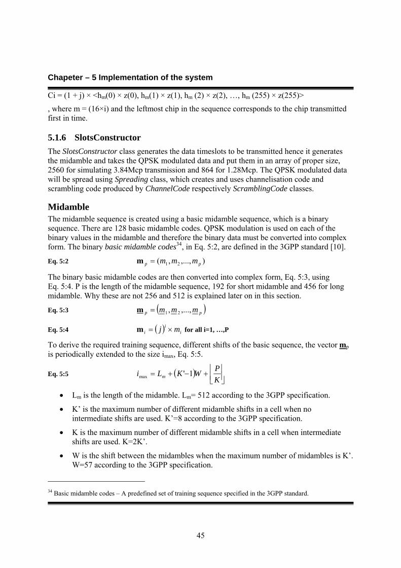
Chapeter – 5 Implementation of the system
45
Ci = (1 + j) × <hm(0) × z(0), hm(1) × z(1), hm (2) × z(2), …, hm (255) × z(255)>
, where m = (16×i) and the leftmost chip in the sequence corresponds to the chip transmitted first in time.
5.1.6 SlotsConstructor The SlotsConstructor class generates the data timeslots to be transmitted hence it generates the midamble and takes the QPSK modulated data and put them in an array of proper size, 2560 for simulating 3.84Mcp transmission and 864 for 1.28Mcp. The QPSK modulated data will be spread using Spreading class, which creates and uses channelisation code and scrambling code produced by ChannelCode respectively ScramblingCode classes.
Midamble The midamble sequence is created using a basic midamble sequence, which is a binary sequence. There are 128 basic midamble codes. QPSK modulation is used on each of the binary values in the midamble and therefore the binary data must be converted into complex form. The binary basic midamble codes34, in Eq. 5:2, are defined in the 3GPP standard [10].
Eq. 5:2 ),...,,( 21 pp mmm=m
The binary basic midamble codes are then converted into complex form, Eq. 5:3, using Eq. 5:4. P is the length of the midamble sequence, 192 for short midamble and 456 for long midamble. Why these are not 256 and 512 is explained later on in this section.
Eq. 5:3 ( )pp mmm ,...,, 21=m
Eq. 5:4 ( ) ii
i mj ×=m for all i=1, …,P
To derive the required training sequence, different shifts of the basic sequence, the vector mp is periodically extended to the size imax, Eq. 5:5.
Eq. 5:5 ( ) ⎥⎦⎥
⎢⎣⎢+−+=
KPWKLi m 1'max
• Lm is the length of the midamble. Lm= 512 according to the 3GPP specification.
• K’ is the maximum number of different midamble shifts in a cell when no intermediate shifts are used. K’=8 according to the 3GPP specification.
• K is the maximum number of different midamble shifts in a cell when intermediate shifts are used. K=2K’.
• W is the shift between the midambles when the maximum number of midambles is K’. W=57 according to the 3GPP specification.
34 Basic midamble codes – A predefined set of training sequence specified in the 3GPP standard.
Chapeter – 5 Implementation of the system
46
• ⎣ ⎦x denotes the largest integer smaller or equal to x.
By using the values of Lm, K’, K and W the value of imax can be determined, imax=939. Now a new vector containing the periodic basic midamble sequence, Eq. 5:6, can be created.
Eq. 5:6 ( )max
,...,, 21 immm=m
The first P elements in m are the same as in mp, the following repeat the beginning, Eq. 5:7.
Eq. 5:7 Pii mm −= for the subset i=(P+1), …,imax
Using this periodic midamble sequence m for each shift k a midamble m(k) of length Lm can be derived, Eq. 5:8.
Eq. 5:8 ( ))()(2
)(1
)( ,...,, kL
kkkm
mmm=m
The Lm midamble elements )(kim of m(k) are calculated according to Eq. 5:9.
Eq. 5:9 WkKik
i mm )'()(
−+= with i=1,..,Lm and k=1,…,K’
If intermediate shifts are used the second K’ midambles are determined by Eq. 5:10 and Eq. 5:11.
Eq. 5:10 ⎥⎦⎥
⎢⎣⎢+−−+=
KPWkKi
ki mm )1'(
)( with i=1,…,Lm and k=(K’+1),..,(K-1)
Eq. 5:11 ⎥⎦⎥
⎢⎣⎢+−+=
KPWKi
ki mm )1'(
)( with i=1,…,Lm and k=K
The complex values of the midambles should not be spread or modulated and are passed directly to the pulse-shaping block.
The system can create one midamble sequence and transmit it but the receiver will not use the information in the midamble. This is because the system only has one cell and uses one scrambling code. All the synchronisation needed can be performed by using the primary synchronisation code.
Spreading The length of the spreading codes used in our system is 16 and consists of two parts. The first part is a channelisation code and the other part is a scrambling sequence. How the channelisation and scrambling codes are determined and how you combine them into a spreading code is explained in this section.
Generating the channelisation code
Generating the channelisation code is the first task when creating the spreading code. This is done according to the algorithm described in Figure 3-12. The system use channelisation codes with length 16, Q=16.
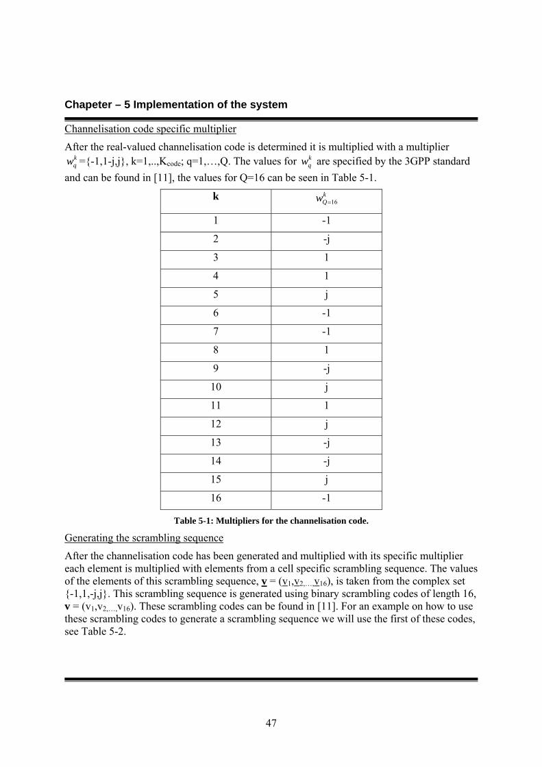
Chapeter – 5 Implementation of the system
47
Channelisation code specific multiplier
After the real-valued channelisation code is determined it is multiplied with a multiplier kqw ={-1,1-j,j}, k=1,..,Kcode; q=1,…,Q. The values for k
qw are specified by the 3GPP standard and can be found in [11], the values for Q=16 can be seen in Table 5-1.
k kQw 16=
1 -1
2 -j
3 1
4 1
5 j
6 -1
7 -1
8 1
9 -j
10 j
11 1
12 j
13 -j
14 -j
15 j
16 -1
Table 5-1: Multipliers for the channelisation code.
Generating the scrambling sequence
After the channelisation code has been generated and multiplied with its specific multiplier each element is multiplied with elements from a cell specific scrambling sequence. The values of the elements of this scrambling sequence, v = (v1,v2,…,v16), is taken from the complex set {-1,1,-j,j}. This scrambling sequence is generated using binary scrambling codes of length 16, v = (v1,v2,…,v16). These scrambling codes can be found in [11]. For an example on how to use these scrambling codes to generate a scrambling sequence we will use the first of these codes, see Table 5-2.
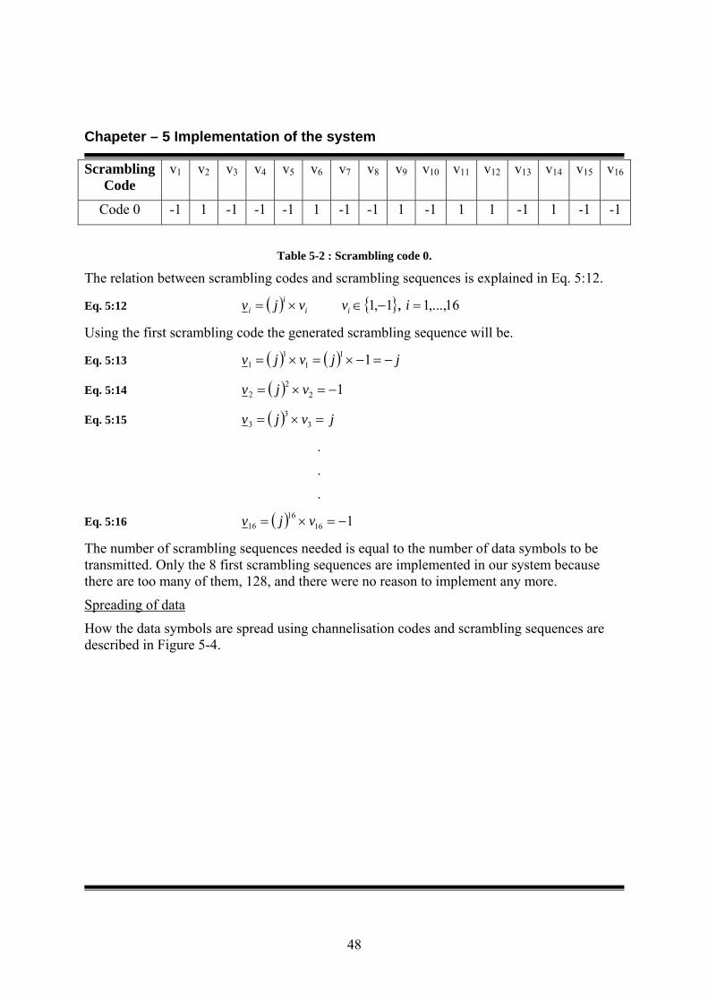
Chapeter – 5 Implementation of the system
48
Scrambling Code
v1 v2 v3 v4 v5 v6 v7 v8 v9 v10 v11 v12 v13 v14 v15 v16
Code 0 -1 1 -1 -1 -1 1 -1 -1 1 -1 1 1 -1 1 -1 -1
Table 5-2 : Scrambling code 0.
The relation between scrambling codes and scrambling sequences is explained in Eq. 5:12.
Eq. 5:12 ( ) ii
i vjv ×= { }1,1 −∈iv , 16,...,1=i
Using the first scrambling code the generated scrambling sequence will be.
Eq. 5:13 ( ) ( ) jjvjv −=−×=×= 111
11
Eq. 5:14 ( ) 122
2 −=×= vjv
Eq. 5:15 ( ) jvjv =×= 33
3
.
.
.
Eq. 5:16 ( ) 11616
16 −=×= vjv
The number of scrambling sequences needed is equal to the number of data symbols to be transmitted. Only the 8 first scrambling sequences are implemented in our system because there are too many of them, 128, and there were no reason to implement any more.
Spreading of data
How the data symbols are spread using channelisation codes and scrambling sequences are described in Figure 5-4.

Chapeter – 5 Implementation of the system
49
Figure 5-4: Spreading the data symbols.
The steps in Figure 5-4 are explained below.
1. These are the modulated data symbols that are to be spread. Nk is the number of data symbols in one timeslot. The i index indicates whether the data bit is transmitted in the first or second data block. Block 1 is transmitted before the midamble and block 2 after. See section 3.5.
2. Each data is multiplied with the channelisation code and weighted with the code specific multiplier.
3. Each spread and weighted data symbol is multiplied with an element of the scrambling sequence. The same scrambling code is used to generate the entire scrambling sequence, which will repeat itself with an interval of 16.
4. The final spread and scrambled data.
The user specific channelisation code and cell specific scrambling sequence can be seen as one user and cell specific spreading code s(k)= ( ))(k
ps with
[ ] [ ]MAXk Qpk
Qpk
p vcs mod)1(1)(
mod)1(1)(
−+−+ ×= k=1, …,KCode and p=1, …,NkQ
Since the system uses one scrambling code to generate the entire cell specific scrambling sequence the algorithm used by the system can be simplified to.
1) ),(1
ikd , ),(2
ikd , … , ),( ikN k
d
( )),(16
),(1 ,..., ikikk
Q ccw × , ( )),(16
),(1 ,..., ikikk
Q ccw × , … , ( )),(16
),(1 ,..., ikikk
Q ccw ×
( )),(1616
),(11
),(1 ,..., ikikikk
Q cvcvdw × , … , ( )),(1616
),(11
),( ,..., ikikikN
kQ cvcvdw
k×
16321 ,...,,, vvvv , 16321 ,...,,, vvvv , … , 16321 ,...,,, vvvv
2)
3)
4)
Chapeter – 5 Implementation of the system
50
Eq. 5:17 [ ] [ ]kk Qpk
Qpk
p vcs mod)1(1)(
mod)1(1)(
−+−+ ×= k=1,…,KCode and p=1,…,NkQ
This means that the NkQ long spreading code consists of Q, Q = 16, elements which is repeated with an interval of Q. Therefore we only use a spreading code with the length Q and loop through it Nk times when spreading.
5.1.7 RCosFilter The RCosFilter class creates an RCOS filter by using Eq. 4:1 from section 4.8. The RCOS filter will be returned as an array containing the sample values of the filter. The size of the filter can be set by the user. If the user does not change the size of the filter the default value of 51 sample values is used.
5.1.8 Upsample The upsample function is used to upsample the data signal by a factor of 4. This needs to be done because of the pulseshaping operation. Upsampling the signal results in a signal more suitable for radio transmission, see section 4.8.
5.1.9 Conv The conv function convolutes two arrays with each other. This function is used for the pulse shaping operation to convolute the upsampled data signal with the RCOS filter.
5.2 Channel This section describes the implementation of the channel and what its features are. The channel simulates a Rayleigh fading channel with up to 5 multipaths. Random noise of different strengths can be added to disturb the signal. The output from the channel will be a phase shifted version of the input with multipaths and noise added. The structure of the channel program can be seen in Figure 5-5.
• channel is the executable file of the channel program. It contains the interface that handles input, output and sets the channel parameters.
• MyChannel contains most of the functionality of the channel. The class phase shifts data, adds noise, adds multipaths and calculates SNR.
• CDMAfunctions o writeToMFile used to write the calculated SNR to a file.
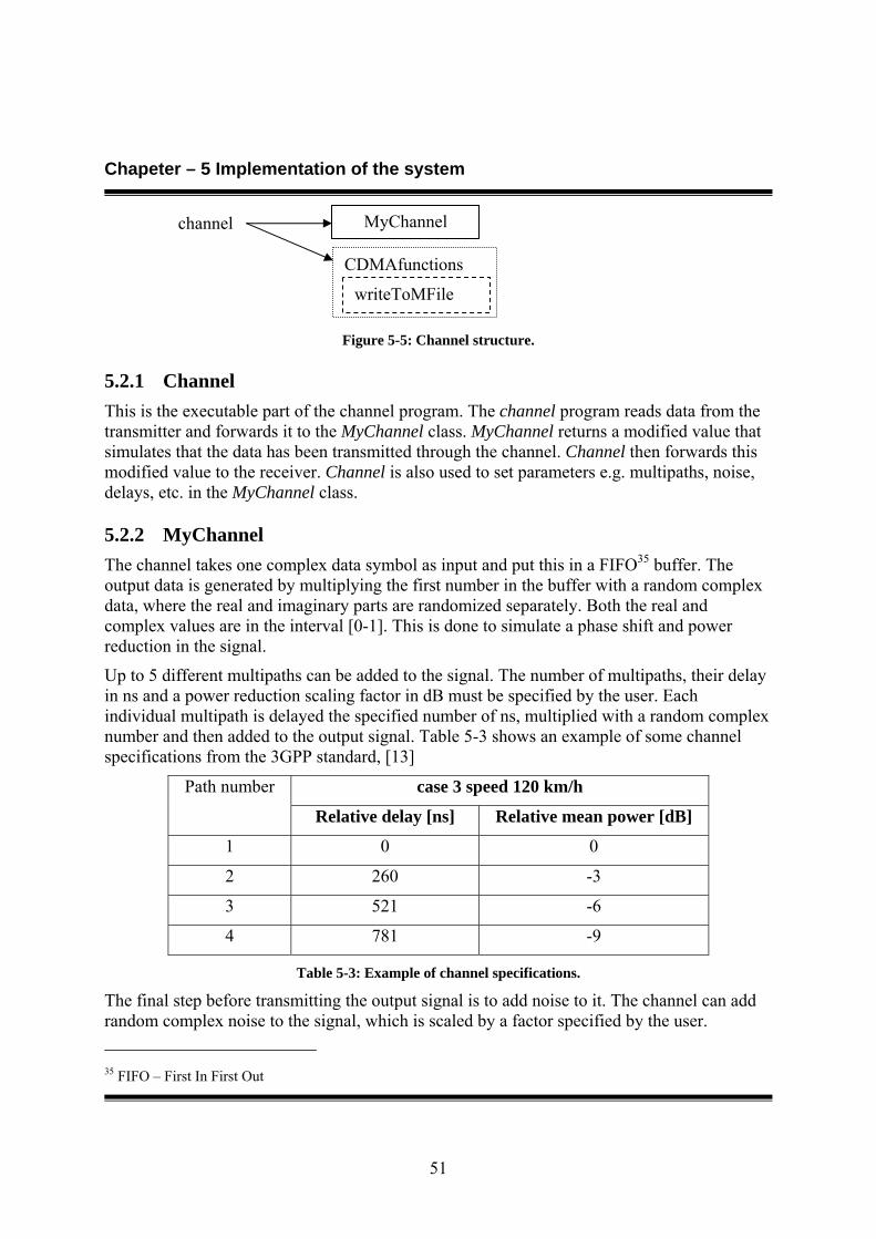
Chapeter – 5 Implementation of the system
51
Figure 5-5: Channel structure.
5.2.1 Channel This is the executable part of the channel program. The channel program reads data from the transmitter and forwards it to the MyChannel class. MyChannel returns a modified value that simulates that the data has been transmitted through the channel. Channel then forwards this modified value to the receiver. Channel is also used to set parameters e.g. multipaths, noise, delays, etc. in the MyChannel class.
5.2.2 MyChannel The channel takes one complex data symbol as input and put this in a FIFO35 buffer. The output data is generated by multiplying the first number in the buffer with a random complex data, where the real and imaginary parts are randomized separately. Both the real and complex values are in the interval [0-1]. This is done to simulate a phase shift and power reduction in the signal.
Up to 5 different multipaths can be added to the signal. The number of multipaths, their delay in ns and a power reduction scaling factor in dB must be specified by the user. Each individual multipath is delayed the specified number of ns, multiplied with a random complex number and then added to the output signal. Table 5-3 shows an example of some channel specifications from the 3GPP standard, [13]
case 3 speed 120 km/h Path number
Relative delay [ns] Relative mean power [dB]
1 0 0
2 260 -3
3 521 -6
4 781 -9
Table 5-3: Example of channel specifications.
The final step before transmitting the output signal is to add noise to it. The channel can add random complex noise to the signal, which is scaled by a factor specified by the user. 35 FIFO – First In First Out
channel MyChannel
CDMAfunctions
writeToMFile
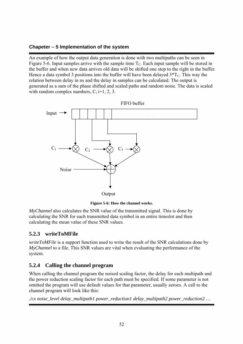
Chapeter – 5 Implementation of the system
52
An example of how the output data generation is done with two multipaths can be seen in Figure 5-6. Input samples arrive with the sample time TC. Each input sample will be stored in the buffer and when new data arrives old data will be shifted one step to the right in the buffer. Hence a data symbol 3 positions into the buffer will have been delayed 3*TC. This way the relation between delay in ns and the delay in samples can be calculated. The output is generated as a sum of the phase shifted and scaled paths and random noise. The data is scaled with random complex numbers, Ci i=1, 2, 3.
Figure 5-6: How the channel works.
MyChannel also calculates the SNR value of the transmitted signal. This is done by calculating the SNR for each transmitted data symbol in an entire timeslot and then calculating the mean value of these SNR values.
5.2.3 writeToMFile writeToMFile is a support function used to write the result of the SNR calculations done by MyChannel to a file. This SNR values are vital when evaluating the performance of the system.
5.2.4 Calling the channel program When calling the channel program the noised scaling factor, the delay for each multipath and the power reduction scaling factor for each path must be specified. If some parameter is not omitted the program will use default values for that parameter, usually zeroes. A call to the channel program will look like this:
./cx noise_level delay_multipath1 power_reduction1 delay_multipath2 power_reduction2 …
Input
FIFO buffer
. . .
C1 C2 C3
Noise
Output
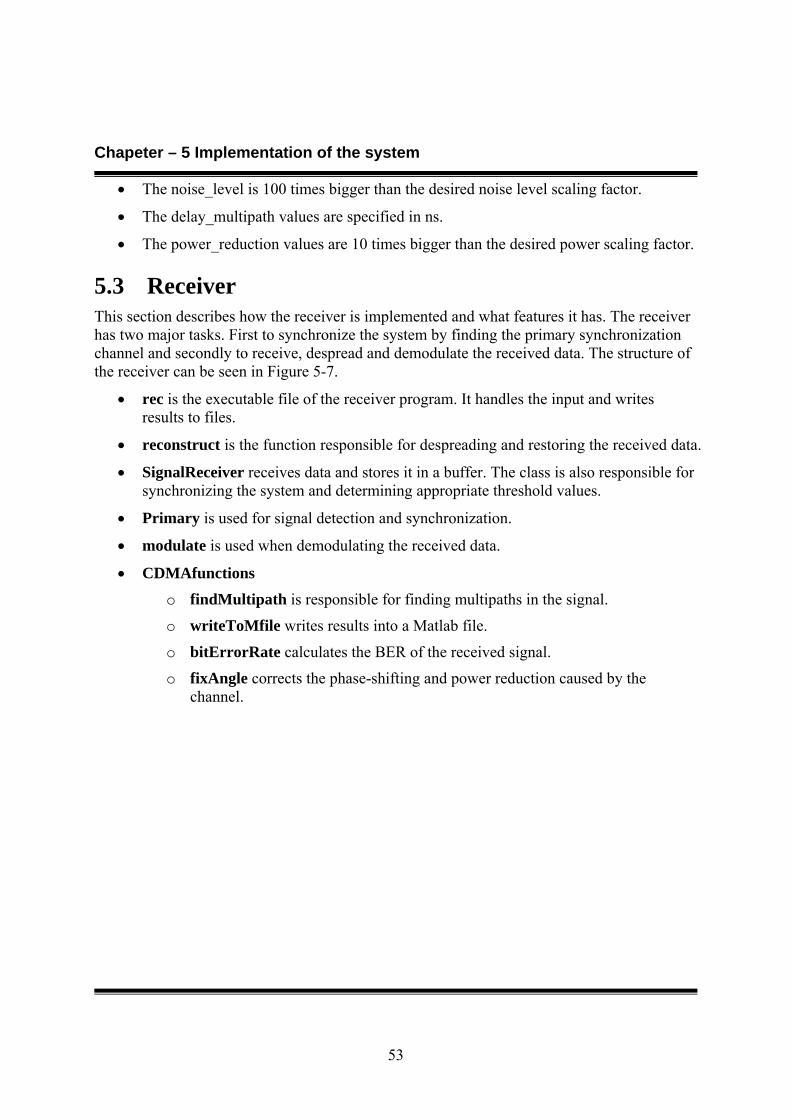
Chapeter – 5 Implementation of the system
53
• The noise_level is 100 times bigger than the desired noise level scaling factor.
• The delay_multipath values are specified in ns.
• The power_reduction values are 10 times bigger than the desired power scaling factor.
5.3 Receiver This section describes how the receiver is implemented and what features it has. The receiver has two major tasks. First to synchronize the system by finding the primary synchronization channel and secondly to receive, despread and demodulate the received data. The structure of the receiver can be seen in Figure 5-7.
• rec is the executable file of the receiver program. It handles the input and writes results to files.
• reconstruct is the function responsible for despreading and restoring the received data.
• SignalReceiver receives data and stores it in a buffer. The class is also responsible for synchronizing the system and determining appropriate threshold values.
• Primary is used for signal detection and synchronization.
• modulate is used when demodulating the received data.
• CDMAfunctions o findMultipath is responsible for finding multipaths in the signal.
o writeToMfile writes results into a Matlab file.
o bitErrorRate calculates the BER of the received signal.
o fixAngle corrects the phase-shifting and power reduction caused by the channel.
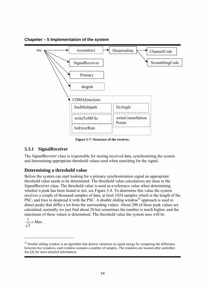
Chapeter – 5 Implementation of the system
54
Figure 5-7: Structure of the receiver.
5.3.1 SignalReceiver The SignalReceiver class is responsible for storing received data, synchronising the system and determining appropriate threshold values used when searching for the signal.
Determining a threshold value Before the system can start looking for a primary synchronization signal an appropriate threshold value needs to be determined. The threshold value calculations are done in the SignalReceiver class. The threshold value is used as a reference value when determining whether a peak has been found or not, see Figure 5-8. To determine this value the system receives a couple of thousand samples of data, at least 1024 samples which is the length of the PSC, and tries to despread it with the PSC. A double sliding window36 approach is used to detect peaks that differ a lot from the surrounding values. About 200 of these peak values are calculated, normally we just find about 20 but sometimes the number is much higher, and the maximum of these values is determined. The threshold value the system uses will be
Max×2
1 .
36 Double sliding window is an algorithm that detects variations in signal energy by comparing the difference between two windows, each window contains a number of samples. The windows are located after eachother. See [8] for more detailed information.
CDMAfunctions
bitErrorRate
findMultipath
writeToMFile writeConstellationPoints
SignalReceiver
Primary
reconstruct
deqpsk
Despreading
ScramblingCode
ChannelCode
fixAngle
rec
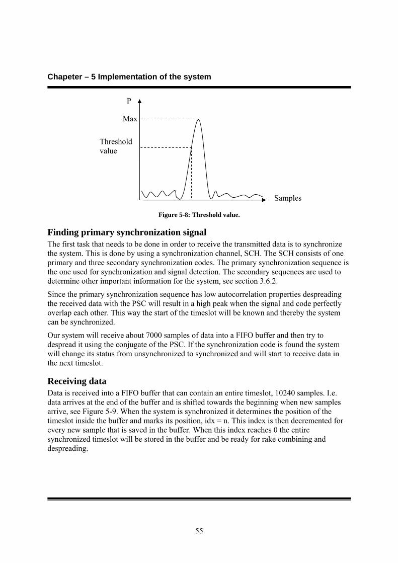
Chapeter – 5 Implementation of the system
55
Figure 5-8: Threshold value.
Finding primary synchronization signal The first task that needs to be done in order to receive the transmitted data is to synchronize the system. This is done by using a synchronization channel, SCH. The SCH consists of one primary and three secondary synchronization codes. The primary synchronization sequence is the one used for synchronization and signal detection. The secondary sequences are used to determine other important information for the system, see section 3.6.2.
Since the primary synchronization sequence has low autocorrelation properties despreading the received data with the PSC will result in a high peak when the signal and code perfectly overlap each other. This way the start of the timeslot will be known and thereby the system can be synchronized.
Our system will receive about 7000 samples of data into a FIFO buffer and then try to despread it using the conjugate of the PSC. If the synchronization code is found the system will change its status from unsynchronized to synchronized and will start to receive data in the next timeslot.
Receiving data Data is received into a FIFO buffer that can contain an entire timeslot, 10240 samples. I.e. data arrives at the end of the buffer and is shifted towards the beginning when new samples arrive, see Figure 5-9. When the system is synchronized it determines the position of the timeslot inside the buffer and marks its position, idx = n. This index is then decremented for every new sample that is saved in the buffer. When this index reaches 0 the entire synchronized timeslot will be stored in the buffer and be ready for rake combining and despreading.
P
Threshold value
Samples
Max
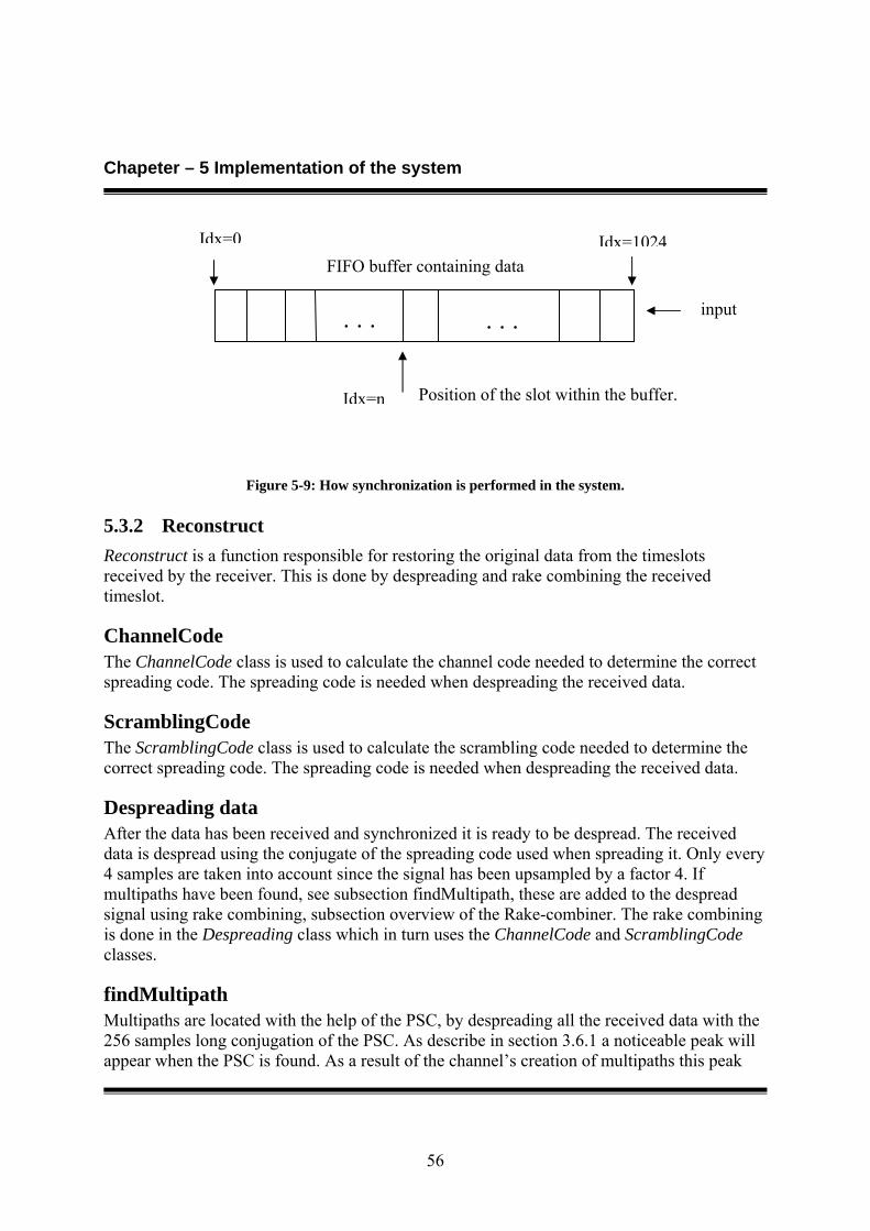
Chapeter – 5 Implementation of the system
56
Figure 5-9: How synchronization is performed in the system.
5.3.2 Reconstruct Reconstruct is a function responsible for restoring the original data from the timeslots received by the receiver. This is done by despreading and rake combining the received timeslot.
ChannelCode The ChannelCode class is used to calculate the channel code needed to determine the correct spreading code. The spreading code is needed when despreading the received data.
ScramblingCode The ScramblingCode class is used to calculate the scrambling code needed to determine the correct spreading code. The spreading code is needed when despreading the received data.
Despreading data After the data has been received and synchronized it is ready to be despread. The received data is despread using the conjugate of the spreading code used when spreading it. Only every 4 samples are taken into account since the signal has been upsampled by a factor 4. If multipaths have been found, see subsection findMultipath, these are added to the despread signal using rake combining, subsection overview of the Rake-combiner. The rake combining is done in the Despreading class which in turn uses the ChannelCode and ScramblingCode classes.
findMultipath Multipaths are located with the help of the PSC, by despreading all the received data with the 256 samples long conjugation of the PSC. As describe in section 3.6.1 a noticeable peak will appear when the PSC is found. As a result of the channel’s creation of multipaths this peak
. . . . . .
FIFO buffer containing data
input
Position of the slot within the buffer. Idx=n
Idx=0 Idx=1024
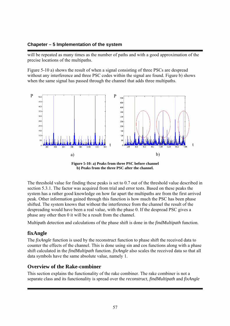
Chapeter – 5 Implementation of the system
57
will be repeated as many times as the number of paths and with a good approximation of the precise locations of the multipaths.
Figure 5-10 a) shows the result of when a signal consisting of three PSCs are despread without any interference and three PSC codes within the signal are found. Figure b) shows when the same signal has passed through the channel that adds three multipaths.
Figure 5-10: a) Peaks from three PSC before channel
b) Peaks from the three PSC after the channel.
The threshold value for finding these peaks is set to 0.7 out of the threshold value described in section 5.3.1. The factor was acquired from trial and error tests. Based on these peaks the system has a rather good knowledge on how far apart the multipaths are from the first arrived peak. Other information gained through this function is how much the PSC has been phase shifted. The system knows that without the interference from the channel the result of the despreading would have been a real value, with the phase 0. If the despread PSC gives a phase any other then 0 it will be a result from the channel.
Multipath detection and calculations of the phase shift is done in the findMultipath function.
fixAngle The fixAngle function is used by the reconstruct function to phase shift the received data to counter the effects of the channel. This is done using sin and cos functions along with a phase shift calculated in the findMultipath function. fixAngle also scales the received data so that all data symbols have the same absolute value, namely 1.
Overview of the Rake-combiner This section explains the functionality of the rake combiner. The rake combiner is not a separate class and its functionality is spread over the reconstruct, findMultipath and fixAngle
a) b)
P
t t
P

Chapeter – 5 Implementation of the system
58
functions. Therefore this section tries to explain in more detail how the rake combiner functions.
The reconstruct function uses the information gained from the findMultipath function to rebuild the original transmitted data signal. An illustration of the procedure can be observed in Figure 5-11.
Figure 5-11: Example of a rake with 4 fingers.
First the received signal, rs, is split into a specific number of rake fingers. This value can be set to be between {1-6}. Each of the signals passes through a time delay device so that the multipath signals are synchronized and arrive at the same time as the first signal. This is followed by a multiplier, which multiplies the signal with the conjunction of the spreading code, and a sum operation to despread the data signal. Before all the signals is added together they are separately phase shifted to counter the effect of the phase shifting of the channel, according to the values calculated in the function findMultipath, using the fixAngle function. This is illustrated in Figure 5-11 with a multiplication of a complex value, but in reality the signal is shifted with the help of the mathematical functions sin and cos. Figure 5-12 shows how a data constellation point can change from a) transmission, b) through the channel and c) after the data is reconstructed. In Figure 5-12 b) the phase shifts needed to be corrected are also drawn.
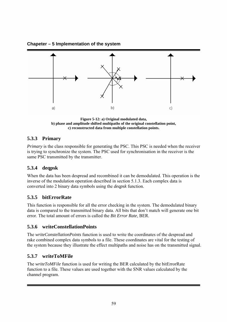
Chapeter – 5 Implementation of the system
59
Figure 5-12: a) Original modulated data,
b) phase and amplitude shifted multipaths of the original constellation point, c) reconstructed data from multiple constellation points.
5.3.3 Primary Primary is the class responsible for generating the PSC. This PSC is needed when the receiver is trying to synchronize the system. The PSC used for synchronisation in the receiver is the same PSC transmitted by the transmitter.
5.3.4 deqpsk When the data has been despread and recombined it can be demodulated. This operation is the inverse of the modulation operation described in section 5.1.3. Each complex data is converted into 2 binary data symbols using the deqpsk function.
5.3.5 bitErrorRate This function is responsible for all the error checking in the system. The demodulated binary data is compared to the transmitted binary data. All bits that don’t match will generate one bit error. The total amount of errors is called the Bit Error Rate, BER.
5.3.6 writeConstellationPoints The writeConstellationPoints function is used to write the coordinates of the despread and rake combined complex data symbols to a file. These coordinates are vital for the testing of the system because they illustrate the effect multipaths and noise has on the transmitted signal.
5.3.7 writeToMFile The writeToMFile function is used for writing the BER calculated by the bitErrorRate function to a file. These values are used together with the SNR values calculated by the channel program.
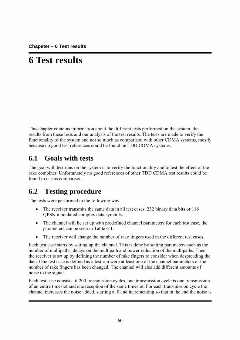
Chapeter – 6 Test results
60
6 Test results
This chapter contains information about the different tests performed on the system, the results from these tests and our analysis of the test results. The tests are made to verify the functionality of the system and not so much as comparison with other CDMA systems, mostly because no good test references could be found on TDD CDMA systems.
6.1 Goals with tests The goal with test runs on the system is to verify the functionality and to test the effect of the rake combiner. Unfortunately no good references of other TDD CDMA test results could be found to use as comparison.
6.2 Testing procedure The tests were performed in the following way.
• The receiver transmits the same data in all test cases, 232 binary data bits or 116 QPSK modulated complex data symbols.
• The channel will be set up with predefined channel parameters for each test case, the parameters can be seen in Table 6-1.
• The receiver will change the number of rake fingers used in the different test cases.
Each test case starts by setting up the channel. This is done by setting parameters such as the number of multipaths, delays on the multipath and power reduction of the multipaths. Then the receiver is set up by defining the number of rake fingers to consider when despreading the data. One test case is defined as a test run were at least one of the channel parameters or the number of rake fingers has been changed. The channel will also add different amounts of noise to the signal.
Each test case consists of 200 transmission cycles, one transmission cycle is one transmission of an entire timeslot and one reception of the same timeslot. For each transmission cycle the channel increases the noise added, starting at 0 and incrementing so that in the end the noise is

Chapeter – 6 Test results
61
much stronger then the signal. By slowly increasing the noise added a good understanding on how interference will affect the performance of the system is achieved. Since the noise will be randomized for each data symbol transmitted through the channel the affect of the noise added can differ quite a lot from symbol to symbol. If unlucky this can cause unexpected bit errors even with a quite strong signal.
The different channel parameters used when testing our systems are specified in the 3GPP standard, [13]. For tests with up to 4 paths, 3 multipaths, we used the test case 3 speed 120 km/h from [13], see Table 6-1. For tests with up to 6 paths, 5 multipaths, we used the test ITU vehicular A Speed 30km/h (VA30) from [13], see Table 6-1. Case 3 speed 120 km/h simulates a that the receiver, mobile phone, is moving at 120km/h, e.g. driving a car. ITU vehicular A Speed 30km/h (VA30) simulates a vehicular travelling at 30km/h, e.g. driving a car or riding a bike.
case 3 speed 120 km/h ITU vehicular A Speed 30km/h (VA30)
Path number
Relative delay [ns]
Relative mean power [dB]
Relative delay [ns]
Relative mean power [dB]
1 0 0 0 0
2 260 -3 310 -1
3 521 -6 710 -9
4 781 -9 1090 -10
5 - - 1730 -15
6 - - 2510 -20
Table 6-1: Test cases.
All of the test cases using 1-4 paths were run using case 3 from Table 6-1. This because case 3 is a good representative of the test cases defined in [13], it is also one of the most challenging cases with strong multipaths.
In the test with 6 paths only two test cases were run, the cases of using 6 multipaths and 5 or 6 rake fingers. This is because cases using less fingers and multipaths have already been tested in the test cases using 4 paths. All the test cases defined in [13] using 5 or more paths also have a very high power reduction of the multipaths making them undetectable by the system. This is another reason why not doing more tests on the 6 paths case, since only the first paths can be found running several tests on these cases will only give the same result.
6.3 Presenting the test results The results from the test runs are displayed using the constellation points of the despread and rake combined signal. This is because the location of the constellation points gives a good understanding on how interference actually affects the system. Each constellation point
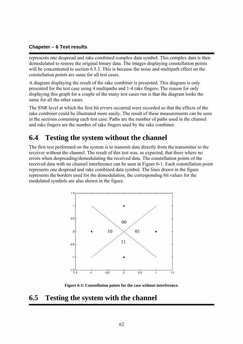
Chapeter – 6 Test results
62
represents one despread and rake combined complex data symbol. This complex data is then demodulated to restore the original binary data. The images displaying constellation points will be concentrated to section 6.5.3. This is because the noise and multipath effect on the constellation points are same for all test cases.
A diagram displaying the result of the rake combiner is presented. This diagram is only presented for the test case using 4 multipaths and 1-4 rake fingers. The reason for only displaying this graph for a couple of the many test cases run is that the diagram looks the same for all the other cases.
The SNR level at which the first bit errors occurred were recorded so that the effects of the rake combiner could be illustrated more easily. The result of these measurements can be seen in the sections containing each test case. Paths are the number of paths used in the channel and rake fingers are the number of rake fingers used by the rake combiner.
6.4 Testing the system without the channel The first test performed on the system is to transmit data directly from the transmitter to the receiver without the channel. The result of this test was, as expected, that there where no errors when despreading/demodulating the received data. The constellation points of the received data with no channel interference can be seen in Figure 6-1. Each constellation point represents one despread and rake combined data symbol. The lines drawn in the figure represents the borders used for the demodulation, the corresponding bit values for the modulated symbols are also shown in the figure.
Figure 6-1: Constellation points for the case without interference.
6.5 Testing the system with the channel
00
10
11
01

Chapeter – 6 Test results
63
The next series of tests is performed using the channel between the transmitter and receiver. The number of multipaths and the level of noise added were modified to get a good picture of how well the system could handle interference and multipath problems.
The test results for all the tests will give very similar figures and graphs. Because of this the section that covers 4 multipaths will have the most detailed information from the tests and the other test cases will refer to the this section instead of drawing the same images all over again. We chose to present the section with 4 multipaths since it was a good representative of the other test cases.
6.5.1 Using only 1 path Paths Rake fingers First error occurrence
(SNR in dB)
1 1 0,03
Table 6-2: Test parameters for the case with 1 path.
The first test used only one path in the channel, the first path in the case 3 speed 120 km/h. The path is still phase shifted and had its signal power modified. The received signal was decoded with a good result. The first errors occurred at SNR=0,03 which means there is almost as much noise energy as signal energy in the channel. The fact that the systems can receive a signal with as much interference energy as signal energy is an acceptable result.
6.5.2 Using 2 or 3 paths Paths Rake fingers First error occurrence
(SNR in dB)
2 1 2,5
2 2 0,6
3 1 3,7
3 2 0,05
3 3 -1
Table 6-3: Test parameters for the case with 2 or 3 paths.
The results from using 2 or 3 paths are very similar and show small variations between them. Using more rake fingers results in a system that can withstand more interference. The reason why a system with a rake combiner in a multipath environment can be even better than the system in a multipath free environment is that the extra paths will add energy to the received signal when combined. Since the test results from these tests follow the same pattern as the
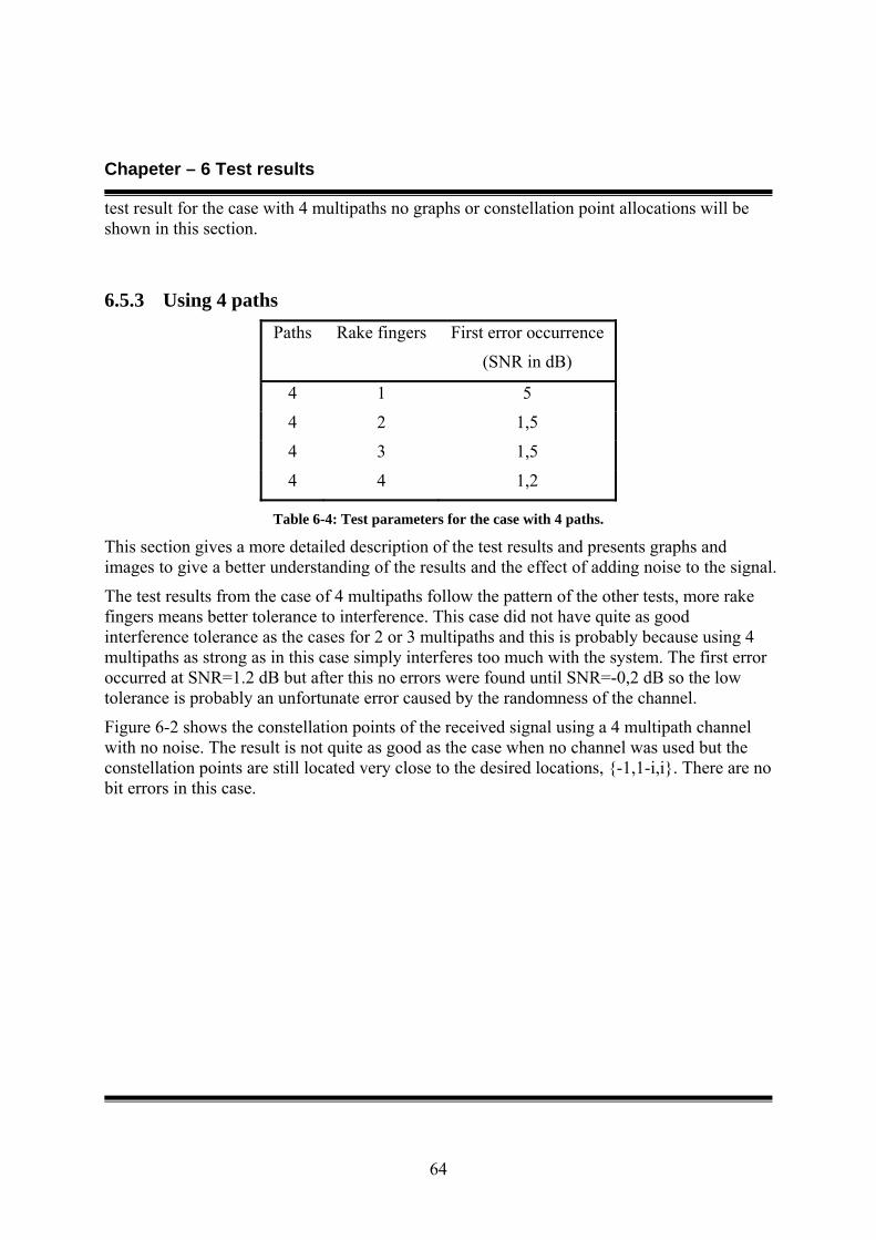
Chapeter – 6 Test results
64
test result for the case with 4 multipaths no graphs or constellation point allocations will be shown in this section.
6.5.3 Using 4 paths Paths Rake fingers First error occurrence
(SNR in dB)
4 1 5
4 2 1,5
4 3 1,5
4 4 1,2
Table 6-4: Test parameters for the case with 4 paths.
This section gives a more detailed description of the test results and presents graphs and images to give a better understanding of the results and the effect of adding noise to the signal.
The test results from the case of 4 multipaths follow the pattern of the other tests, more rake fingers means better tolerance to interference. This case did not have quite as good interference tolerance as the cases for 2 or 3 multipaths and this is probably because using 4 multipaths as strong as in this case simply interferes too much with the system. The first error occurred at SNR=1.2 dB but after this no errors were found until SNR=-0,2 dB so the low tolerance is probably an unfortunate error caused by the randomness of the channel.
Figure 6-2 shows the constellation points of the received signal using a 4 multipath channel with no noise. The result is not quite as good as the case when no channel was used but the constellation points are still located very close to the desired locations, {-1,1-i,i}. There are no bit errors in this case.
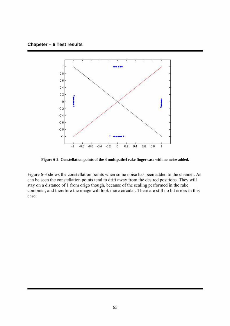
Chapeter – 6 Test results
65
Figure 6-2: Constellation points of the 4 multipath/4 rake finger case with no noise added.
Figure 6-3 shows the constellation points when some noise has been added to the channel. As can be seen the constellation points tend to drift away from the desired positions. They will stay on a distance of 1 from origo though, because of the scaling performed in the rake combiner, and therefore the image will look more circular. There are still no bit errors in this case.
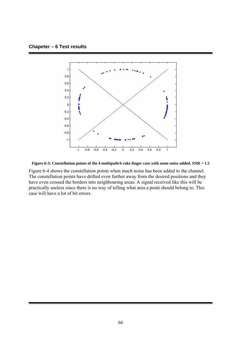
Chapeter – 6 Test results
66
Figure 6-3: Constellation points of the 4 multipath/4 rake finger case with some noise added. SNR = 1.5
Figure 6-4 shows the constellation points when much noise has been added to the channel. The constellation points have drifted even further away from the desired positions and they have even crossed the borders into neighbouring areas. A signal received like this will be practically useless since there is no way of telling what area a point should belong to. This case will have a lot of bit errors.
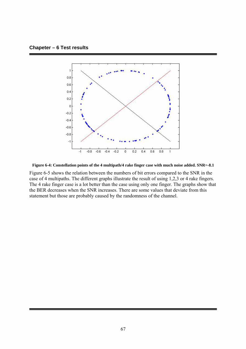
Chapeter – 6 Test results
67
Figure 6-4: Constellation points of the 4 multipath/4 rake finger case with much noise added. SNR=-8.1
Figure 6-5 shows the relation between the numbers of bit errors compared to the SNR in the case of 4 multipaths. The different graphs illustrate the result of using 1,2,3 or 4 rake fingers. The 4 rake finger case is a lot better than the case using only one finger. The graphs show that the BER decreases when the SNR increases. There are some values that deviate from this statement but those are probably caused by the randomness of the channel.
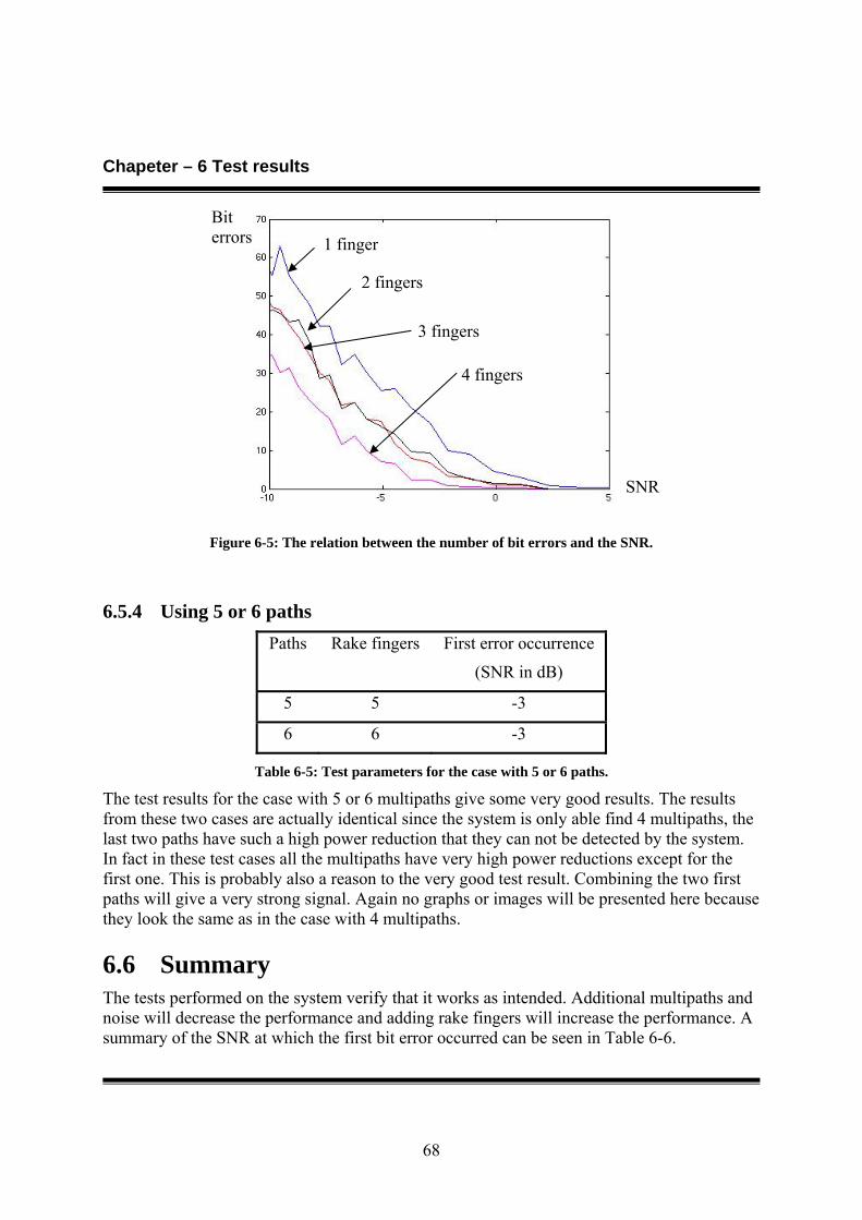
Chapeter – 6 Test results
68
Figure 6-5: The relation between the number of bit errors and the SNR.
6.5.4 Using 5 or 6 paths Paths Rake fingers First error occurrence
(SNR in dB)
5 5 -3
6 6 -3
Table 6-5: Test parameters for the case with 5 or 6 paths.
The test results for the case with 5 or 6 multipaths give some very good results. The results from these two cases are actually identical since the system is only able find 4 multipaths, the last two paths have such a high power reduction that they can not be detected by the system. In fact in these test cases all the multipaths have very high power reductions except for the first one. This is probably also a reason to the very good test result. Combining the two first paths will give a very strong signal. Again no graphs or images will be presented here because they look the same as in the case with 4 multipaths.
6.6 Summary The tests performed on the system verify that it works as intended. Additional multipaths and noise will decrease the performance and adding rake fingers will increase the performance. A summary of the SNR at which the first bit error occurred can be seen in Table 6-6.
3 fingers
1 finger
SNR
Bit errors
4 fingers
2 fingers
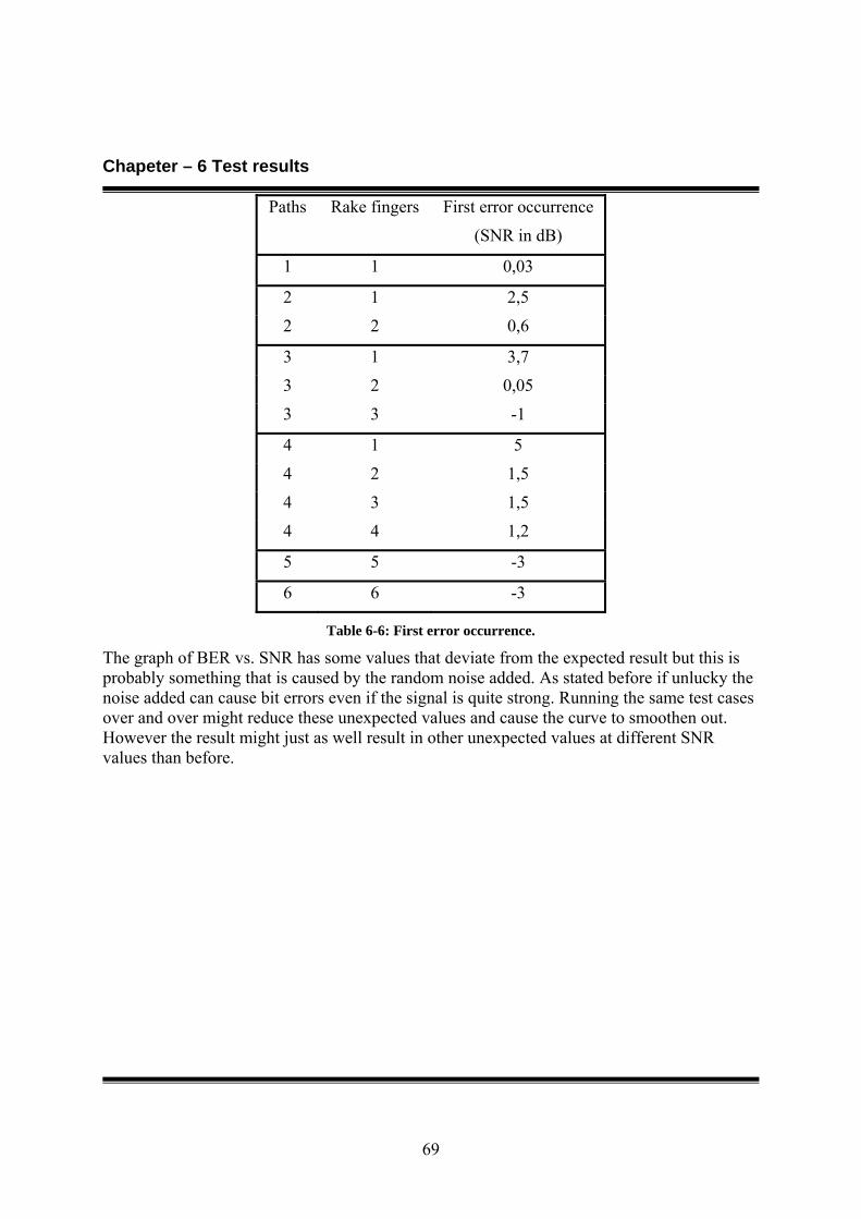
Chapeter – 6 Test results
69
Paths Rake fingers First error occurrence
(SNR in dB)
1 1 0,03
2 1 2,5
2 2 0,6
3 1 3,7
3 2 0,05
3 3 -1
4 1 5
4 2 1,5
4 3 1,5
4 4 1,2
5 5 -3
6 6 -3
Table 6-6: First error occurrence.
The graph of BER vs. SNR has some values that deviate from the expected result but this is probably something that is caused by the random noise added. As stated before if unlucky the noise added can cause bit errors even if the signal is quite strong. Running the same test cases over and over might reduce these unexpected values and cause the curve to smoothen out. However the result might just as well result in other unexpected values at different SNR values than before.
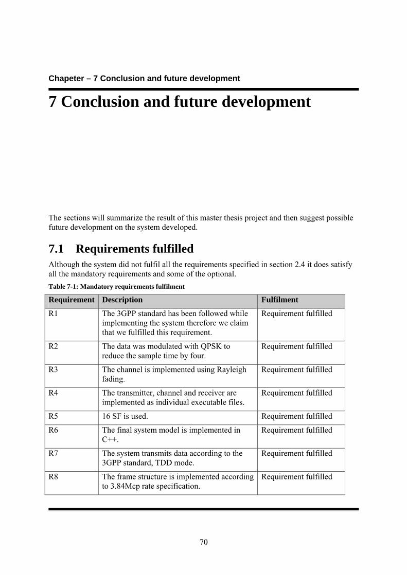
Chapeter – 7 Conclusion and future development
70
7 Conclusion and future development
The sections will summarize the result of this master thesis project and then suggest possible future development on the system developed.
7.1 Requirements fulfilled Although the system did not fulfil all the requirements specified in section 2.4 it does satisfy all the mandatory requirements and some of the optional. Table 7-1: Mandatory requirements fulfilment
Requirement Description Fulfilment
R1 The 3GPP standard has been followed while implementing the system therefore we claim that we fulfilled this requirement.
Requirement fulfilled
R2 The data was modulated with QPSK to reduce the sample time by four.
Requirement fulfilled
R3 The channel is implemented using Rayleigh fading.
Requirement fulfilled
R4 The transmitter, channel and receiver are implemented as individual executable files.
Requirement fulfilled
R5 16 SF is used. Requirement fulfilled
R6 The final system model is implemented in C++.
Requirement fulfilled
R7 The system transmits data according to the 3GPP standard, TDD mode.
Requirement fulfilled
R8 The frame structure is implemented according to 3.84Mcp rate specification.
Requirement fulfilled
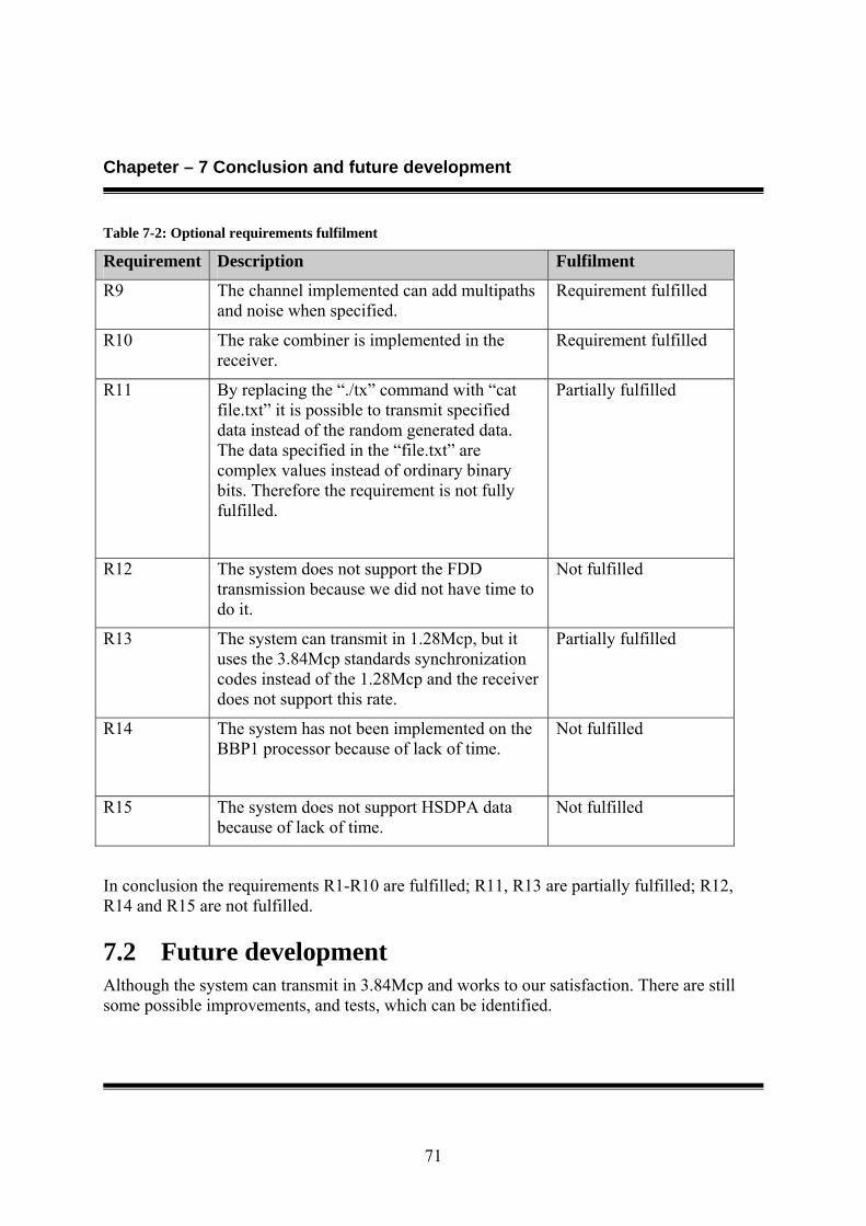
Chapeter – 7 Conclusion and future development
71
Table 7-2: Optional requirements fulfilment
Requirement Description Fulfilment
R9 The channel implemented can add multipaths and noise when specified.
Requirement fulfilled
R10 The rake combiner is implemented in the receiver.
Requirement fulfilled
R11 By replacing the “./tx” command with “cat file.txt” it is possible to transmit specified data instead of the random generated data. The data specified in the “file.txt” are complex values instead of ordinary binary bits. Therefore the requirement is not fully fulfilled.
Partially fulfilled
R12 The system does not support the FDD transmission because we did not have time to do it.
Not fulfilled
R13 The system can transmit in 1.28Mcp, but it uses the 3.84Mcp standards synchronization codes instead of the 1.28Mcp and the receiver does not support this rate.
Partially fulfilled
R14 The system has not been implemented on the BBP1 processor because of lack of time.
Not fulfilled
R15 The system does not support HSDPA data because of lack of time.
Not fulfilled
In conclusion the requirements R1-R10 are fulfilled; R11, R13 are partially fulfilled; R12, R14 and R15 are not fulfilled.
7.2 Future development Although the system can transmit in 3.84Mcp and works to our satisfaction. There are still some possible improvements, and tests, which can be identified.
Chapeter – 7 Conclusion and future development
72
• Even though tested and confirmed that it is possible for different users to transmit in the same timeslot with Matlab, we never got the time to implement such test in the C++ version.
• Our modulation algorithm support for modulation in QPSK, that we used, and 16-QAM, but we did not have time to implement a demodulator for 16-QAM. Using the 16-QAM the system would have increased the data transmission rate with a factor 4 instead of 2.
• The system implemented has no use of the secondary SCH codes because there is no need for the information that can be extracted from these code. The information that could be gained from the secondary SCH was:
o What code group the base station belong to. We only use one base station so this information is not needed.
o Position of a frame within an interleaving period. The system does not use interleaving.
o toffset that specifies where the synchronisation codes are located within a timeslot. toffset is always 0 in the system.
So adding an interleaver or support for multiple base stations will make the secondary SCH codes useful.
• Adding some kind of error correction algorithm, such as SEC ECC, to reduce the BER would be beneficial.
• The system uses only one midamble code sequence which is not used. Adding support for synchronisation using midambles would benefit the system. Adding support for multiple base stations would create the need for more midamble sequences.
• Adding support for FDD transmission mode and compare FDD with TDD could be very interesting.
• The system uses pure C++ data types which causes no accuracy problems. By creating a bit true model of the system to simulate real hardware problems with limited bit representation of data types would greatly benefit a future implementation on a DSP.
• Implement the simulated system on a DSP, e.g. BBP1. Implementing the system on hardware would be the ultimate goal for the system.
Appendix
73
Appendix A – References
[1] GSM World, 1999-2000, Fakta om mobiltelefoni, [Online], available from: http://www.gsmworld.net/swedish_stuff/mobiltelefoni_info.htm [accessed 7 February 2005]
[2] Emerging standard & protocols, Xilinx W-CDMA [online], available from: http://www.xilinx.com/esp/wireless/collateral/WCDMA_esp.pdf [accessed 12 February 2005]
[3] searchMobileComputing.com, 2004, W-CDMA [online], available from:
http://searchmobilecomputing.techtarget.com/sDefinition/0,,sid40_gci505610,00.html [accessed 12 February 2005]
[4] Real World Technologies, 2002, Single-bit Error Correction Error Correcting Code (SEC ECC) [online], available from:
http://www.realworldtech.com/page.cfm?ArticleID=RWT121603153445&p=3 [accessed 7 February 2005]
[5] Riaz Esmailzadeh and Masao Nakagawa, 2003, TDD-CDMA for wireless communications, Artech House Publishers, Boston, London
[6] Gordon L. Stüber, 2001, Principles of Mobile Communication, Kluwer Academic Publishers, Norwell, MA, USA
[7] Reliable Software, Cyclic Redundancy Check [online], available from: http://www.relisoft.com/Science/CrcMath.html [accessed 8 February 2005]
[8] Juha Heiskala and John Terry, 2001, OFDM wireless LANs A theoretical and practical guide, Pearson Education
[9] Sune Söderkvist, 1998, Formler och Tabeller, third edition, Erik Larsson AB.
[10] 3GPP, TS 25.221 v6.0.0 Physical channels and mapping of transport channels onto physical channels (TDD) [online], available from http://www.3gpp.org/ftp/Specs/html-info/25221.htm [accessed continously between 20 august 2004 and 1 february 2005].
[11] 3GPP, TS 25.222 v6.0.0 Multiplexing and channel coding (TDD) [online], available from: http://www.3gpp.org/ftp/Specs/html-info/25222.htm , [accessed continously between 20
[12] 3GPP, TS 25.223 v6.0.0 Spreading and modulation (TDD) [online], available from: http://www.3gpp.org/ftp/Specs/html-info/25223.htm , [accessed continously between 20 August 2004 and 1 February 2005].
[13] 3GPP, TS 25.102 v6.0.0 User Equipment(UE) radio transmission and reception (TDD) [online], available from: http://www.3gpp.org/ftp/Specs/html-info/25102.htm , [accessed continously between 20 August 2004 and 1 February 2005].
Appendix
74
[14] Andrew J. Viterbi, 1995, CDMA Principles of spread spectrum communication, ADDISON-WESLEY, Reading, Massachusetts.
[15] Tero Ojanperä and Ramjee Prasad, 1998, Wideband CDMA for third generation mobile communications, Artech House Publishers, Boston, London.
[16] Mathworld, 1999, Rayleigh Distribution [online], available from: http://mathworld.wolfram.com/RayleighDistribution.html [accessed 8 February 2005]
Appendix
75
Appendix B – User manual For the users of the system there are three executable files available to interact with. The commands to run these files are “./tx”, “./cx” and “./rx”.
The first command in the order “./tx” is for running the transmitter. There are two parameters available for this command; rate=3.84 and rate=1.28. Transmitting 100x2 timeslots of 3.84Mcp timeslots will be executed if the first parameter is chosen. Using the second available parameter, rate=1.28, will transmit 100x2 timeslots of 1.28Mcp timeslots. Running the command without any parameter transmits using the default setup which is the 3.84Mcp data rate.
The second command “./cx” is for running the channel program. It takes the pipelined sent data signal from the “./tx” program and process it. There a lot of parameter available for this program adding different levels of noise and adding different numbers of multipaths. Below is a simple specification of the program.
./cx noise_level delay_multipath1 power_reduction1 delay_multipath2 power_reduction2 …
noise_level is an integer used for defining the noises power level in dB, the value will be scaled with a factor of 100 in the program. delay_multipath1 is the time delay in ns of the first multipath from the first transmitted path and power_reduction1 is the power reduction of that path in dB scaled with a factor of 10 (meaning -10 is a reduction of the power with 1 dB). The following parameter has the same structure as the first one, time delay first followed with a power reduction factor. As mentioned in section 4.10 the channel can add up to 5 extra multipaths. The reason for the need to scale the parameters is that we wanted float values and we find it easier implementing it this way.
The last command “./rx” runs the receiver program, which takes in the previous pipelined data signal and process it. This one has no parameters at all, it just takes the signal data and tries to restore the intended send data.
Below are some examples of different commands combination.
./tx rate=3.84
Result: sending 3.84Mcp timeslots
./tx rate=1.28 | ./cx 0
Result: sending 1.28Mcp timeslots through the channel without any multipaths and without any noise disturbance, but note that the signal will still be phase shifted and dampened with random factors.
./tx | ./cx 15 260 30 | ./rx
Appendix
76
Result: sending 3.84Mcp timeslots through the channel, the channel phase shift and damped the signal with random factors and then adds a multipath to the signal with a delay of 260ns with 3dB reduction of the original power level. A noise with 0.15 power level is also added for interference purpose.
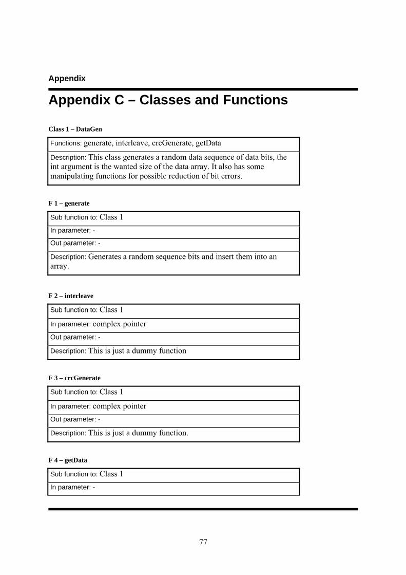
Appendix
77
Appendix C – Classes and Functions Class 1 – DataGen
Functions: generate, interleave, crcGenerate, getData
Description: This class generates a random data sequence of data bits, the int argument is the wanted size of the data array. It also has some manipulating functions for possible reduction of bit errors.
F 1 – generate
Sub function to: Class 1
In parameter: -
Out parameter: -
Description: Generates a random sequence bits and insert them into an array.
F 2 – interleave
Sub function to: Class 1
In parameter: complex pointer Out parameter: -
Description: This is just a dummy function
F 3 – crcGenerate
Sub function to: Class 1
In parameter: complex pointer Out parameter: -
Description: This is just a dummy function.
F 4 – getData
Sub function to: Class 1
In parameter: -
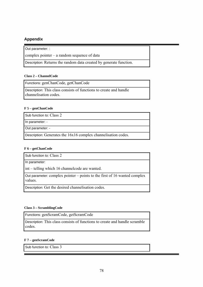
Appendix
78
Out parameter: :
complex pointer – a random sequence of data
Description: Returns the random data created by generate function.
Class 2 – ChannelCode
Functions: genChanCode, getChanCode
Description: This class consists of functions to create and handle channelisation codes.
F 5 – genChanCode
Sub function to: Class 2
In parameter: -
Out parameter: -
Description: Generates the 16x16 complex channelisation codes.
F 6 – getChanCode
Sub function to: Class 2
In parameter:
int – telling which 16 channelcode are wanted.
Out parameter: complex pointer – points to the first of 16 wanted complex values.
Description: Get the desired channelisation codes.
Class 3 – ScramblingCode
Functions: genScramCode, getScramCode
Description: This class consists of functions to create and handle scramble codes.
F 7 – genScramCode
Sub function to: Class 3
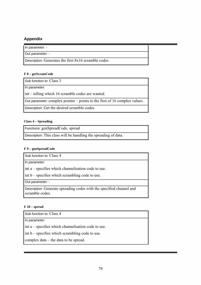
Appendix
79
In parameter: -
Out parameter: -
Description: Generates the first 8x16 scramble codes
F 8 – getScramCode
Sub function to: Class 3
In parameter:
int – telling which 16 scramble codes are wanted.
Out parameter: complex pointer – points to the first of 16 complex values.
Description: Get the desired scramble codes.
Class 4 – Spreading
Functions: genSpreadCode, spread
Description: This class will be handling the spreading of data.
F 9 – genSpreadCode
Sub function to: Class 4
In parameter:
int a – specifies which channelisation code to use.
int b – specifies which scrambling code to use. Out parameter: -
Description: Generate spreading codes with the specified channel and scramble codes.
F 10 – spread
Sub function to: Class 4
In parameter: int a – specifies which channelisation code to use.
int b – specifies which scrambling code to use.
complex data – the data to be spread.
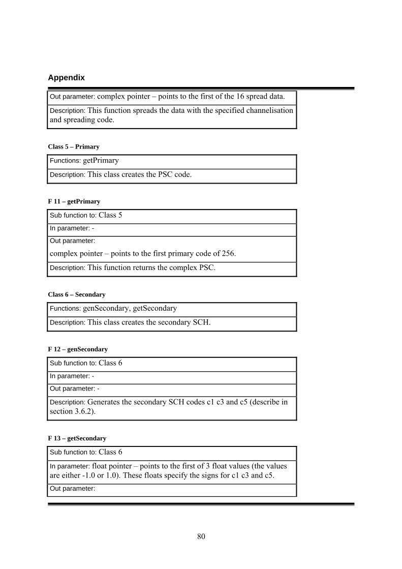
Appendix
80
Out parameter: complex pointer – points to the first of the 16 spread data.
Description: This function spreads the data with the specified channelisation and spreading code.
Class 5 – Primary
Functions: getPrimary
Description: This class creates the PSC code.
F 11 – getPrimary
Sub function to: Class 5
In parameter: -
Out parameter:
complex pointer – points to the first primary code of 256.
Description: This function returns the complex PSC.
Class 6 – Secondary
Functions: genSecondary, getSecondary
Description: This class creates the secondary SCH.
F 12 – genSecondary
Sub function to: Class 6
In parameter: -
Out parameter: -
Description: Generates the secondary SCH codes c1 c3 and c5 (describe in section 3.6.2).
F 13 – getSecondary
Sub function to: Class 6
In parameter: float pointer – points to the first of 3 float values (the values are either -1.0 or 1.0). These floats specify the signs for c1 c3 and c5. Out parameter:

Appendix
81
complex pointer – points to first of 256 long combined SCH.
Description: This function returns the wanted secondary SCH.
Class 7 – SlotsConstuctor
Functions: genMid, createSlot
Description: This class is responsible for handling the creation of slots, both for 3.84 and 1.28 Mcp. The parameter “mode” specifies what kind of slot should be created.
F 14 – genMid
Sub function to: Class 7
In parameter: -
Out parameter: -
Description: Generate midamble and copy it to the created slot.
F 15 – createSlot
Sub function to: Class 7
In parameter:
int a – specifies which channelisation code to use.
int b – specifies which scrambling code to use.
complex pointer – points to the data needed to be spread and put in the created slot. Out parameter:
complex pointer – this pointer points to the created slots.
Description: This function spreads the given data with the stated channelisation and scrambling and puts it in the created slot. This slot can either be a 3.84 or a 1.28 Mcp slot depending on the configuration when created the SlotsConstructor object.
Class 8 – Despreading
Functions: genDeSpreadCode, deSpread

Appendix
82
Description: Handle the despreading of data.
F 16 – genDeSpreadCode
Sub function to: Class 8
In parameter:
int a – specifies which channelisation code to use.
int b – specifies which scrambling code to use.
Out parameter: – void
Description: Generates the despreading code with the specified channelisation and scramble codes.
F 17 – deSpread
Sub function to: Class 8
In parameter:
complex pointer – points to the first of 16 complex values to be despread. Out parameter:
complex data – the data despread from the given 16 complex value.
Description: Despread the data with the given channelisation and scrambling codes.
Class 9 – myChannel
Functions: setupChannel, setChipRate, sendDataThroughChannel, calculateDelay, rayleigh, calculateSNR, setNoise
Description: Class that simulates a rayleigh fading channel. Phase shifts and scales the signal to simulate channel effects. Adds multipaths and noise to the received data and retransmits it. Also calculates SNR. Takes the desired chip rate as in parameter for the constructor, float chip_rate.
F 18 – setupChannel
Sub function to: Class 9
In parameter:
int paths – the number of multipaths desired.

Appendix
83
float power[5] – the power reduction for each path.
float noiselvl – the start value for the noise to be added to the signal.
int delays – the delay for the multipaths in ns.
Out parameter: void
Description: Sets up the original parameters of the channel.
F 19 – setChipRate
Sub function to: Class 9
In parameter:
float chip_rate – the new chip rate for the system
Out parameter: void
Description: Sets a new chip rate for the system. Used when switching from 1.28 to 3.84.
F 20 – sendDataThroughChannel
Sub function to: Class 9
In parameter:
Complex<float> - the data to send through the channel.
Out parameter:
complex<float> - the output from the channel
Description: Sends one complex data through the channel. The output is phase shifted and has multipaths and noise added to it.
F 21 – calculateDelay
Sub function to: Class 9
In parameter:
int delay_ns[5] – the delays in ns.
Out parameter:
int * - pointer to an array of size 5 containing the delays in samples.
Description: Converts delays in ns to delays in samples.
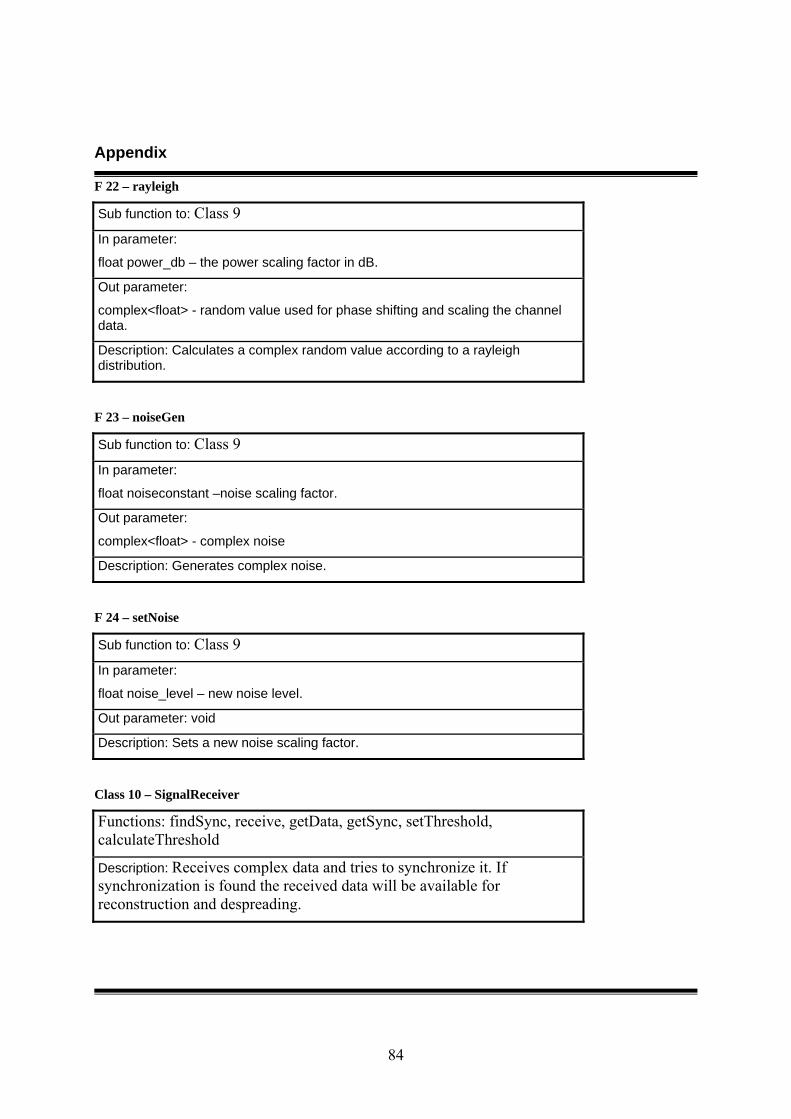
Appendix
84
F 22 – rayleigh
Sub function to: Class 9
In parameter:
float power_db – the power scaling factor in dB.
Out parameter:
complex<float> - random value used for phase shifting and scaling the channel data.
Description: Calculates a complex random value according to a rayleigh distribution.
F 23 – noiseGen
Sub function to: Class 9
In parameter:
float noiseconstant –noise scaling factor.
Out parameter:
complex<float> - complex noise
Description: Generates complex noise.
F 24 – setNoise
Sub function to: Class 9
In parameter:
float noise_level – new noise level.
Out parameter: void
Description: Sets a new noise scaling factor.
Class 10 – SignalReceiver
Functions: findSync, receive, getData, getSync, setThreshold, calculateThreshold
Description: Receives complex data and tries to synchronize it. If synchronization is found the received data will be available for reconstruction and despreading.

Appendix
85
F 25 – findsync
Sub function to: Class 10
In parameter: void
Out parameter:
int – returns 1 if synch is found else 0
Description: Tries to find the PSC by despreading the received data with the conjugate of the PSC.
F 26 – receive
Sub function to: Class 10
In parameter:
complex<float> indata – the data that should be received.
Out parameter:
int – returns 0 if the data is not synchronized and ready. Returns 1 if the data is synchronized and ready.
Description: Receives data from the channel.
F 27 – getSync
Sub function to: Class 10
In parameter: void
Out parameter:
int – returns the synch value. 1 if synched and 0 if not synched.
Description: Returns the synch value.
F 28 – getData
Sub function to: Class 10
In parameter: void
Out parameter:
complex<float> * - the received data buffer.
Description: Returns the entire buffer of received data.
Appendix
86
F 29 – setThreshold
Sub function to: Class 10
In parameter:
float threshold_value – the new threshold value.
Out parameter: void
Description: Sets a new threshold value.
F 30 – calculateThreshold
Sub function to: Class 10
In parameter:
float threshold_value – the scaling factor used when scaling the return value.
Out parameter:
float – the calculated and scaled threshold value
Description: Calculates a threshold value by trying to despread data with the PSC and finding peaks. Scales the highest peak found with the scaling factor.
Class 11 – RcosFilter
Functions: createFilter, getFilter Description: Creates a RCOS filter used for pulseshaping.
F 31 – createFilter
Sub function to: Class 12
In parameter: void
Out parameter: void
Description: Creates an RCOS filter.
F 32 – getfilter
Sub function to: Class 13
In parameter: void
Out parameter:
complex<float> * - pointer to an array containing the filter values.

Appendix
87
Description: Returns an array containing the filter values.
The following functions are not sub-functions to any class. They are support functions used in several parts of the system. F 33 – qpsk
In file: modulate.cc
Parameter:
int * data – pointer to an array of binary data.
int length – the length of the data array.
Return value:
complex<float> * - pointer to an array containing the modulated data.
Description: QPSK modulates an array of binary data.
F 34 – qam16
In file: modulate.cc
Parameter:
int * data – pointer to an array of binary data.
int length – the length of the data array.
Return value:
complex<float> * - pointer to an array containing the modulated data.
Description: 16 QAM modulates an array of binary data.
F 35 – deqpsk
In file: modulate.cc
Parameter:
complex<float> * data – pointer to an array of complex data.
int length – the length of the data array.
Return value:
int * – pointer to an array of binary data.
Description: Demodulates complex data using the QPSK mapping schemes.
F 36 – upsample
In file: cdmafunctions.cc
Appendix
88
Parameter:
complex<float> * data – pointer to an array of data.
int length – the length of the data array.
Return value:
complex<float> * - pointer to an array containing the up sampled data.
Description: up samples a data array with a factor 4.
F 37 – writeToMFile
In file: cdmafunctions
Parameter:
complex<float> * data – pointer to an array of binary data.
int length – the length of the data array.
char * name – filename of the file to write to.
Return value: void
Description: Writes data to a file. There are several write functions but they all work in basically the same way.
F 38 – bitErrorrate
In file: cdmafunctions
Parameter:
int * data – pointer to an array containing the despread and demodulated data.
Return value:
int – the number of bit errors.
Description: Calculates the number of bit errors.
F 39 – writeConsteallationPoints
In file: cdmafunctions.cc
Parameter:
complex<float> * data – pointer to an array of binary data.
int length – the length of the data array.
Return value: void
Description: Writes the coordinates of the constellation points to two different files, xcords.m and ycords.m.

Appendix
89
F 40 – findMultipath
In file: cdmafunctions.cc
Parameter:
complex pointer – points to a data array that may or may not have multipaths
int a – how many fingers the rake have.
float b – the threshold value. Return value:
float pointer – first value of the array states how many multipaths the function manage to find. Then the value comes in a set of 3. First state the position the path was found, second how much the phase of the peak have changed and last the third sates how much the value have damped.
Description: This function calculates the positions of the multipaths and how much the multipaths have changed.
F 41 – fixAngle
In file: cdmafunctions.cc
Parameter:
complex value – complex data that have passed through the channel
float a – the phase the value will be shifted.
float b – the damped factor the function will reverse. Return value:
complex value – complex data, hopefully, without the channels power reduction and phase shift.
Description: The function tries to undo the channels effect on the data.
F 42 – conv
In file: cdmafunctions.cc
Parameter:
complex pointer x – points to arrays that will be convoluted.
int y – size of x.
complex pointer a – points to arrays that will be convoluted.
Appendix
90
int b – size of a. Return value:
complex pointer – points to the convoluted array.
Description: convolutes two arrays of complex values.
F 43 – reconstruct
In file: reconstruct.cc
Parameter:
complex value – complex data that have passed through the channel
float a – the phase the value will be shifted.
float b – the damped factor the function will reverse. Return value:
complex value – rake combined data symbol
Description: The rake function.
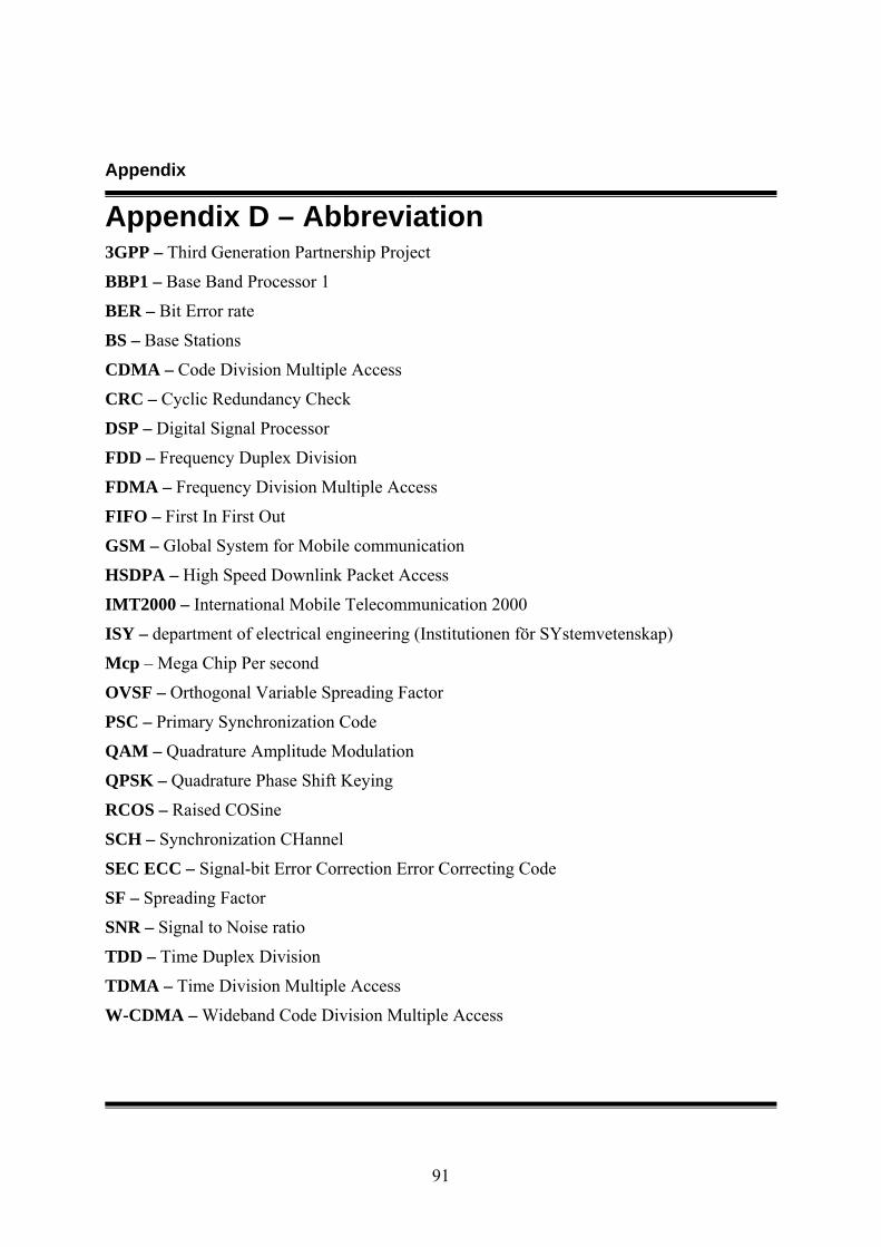
Appendix
91
Appendix D – Abbreviation 3GPP – Third Generation Partnership Project
BBP1 – Base Band Processor 1
BER – Bit Error rate
BS – Base Stations
CDMA – Code Division Multiple Access
CRC – Cyclic Redundancy Check
DSP – Digital Signal Processor
FDD – Frequency Duplex Division
FDMA – Frequency Division Multiple Access
FIFO – First In First Out
GSM – Global System for Mobile communication
HSDPA – High Speed Downlink Packet Access
IMT2000 – International Mobile Telecommunication 2000
ISY – department of electrical engineering (Institutionen för SYstemvetenskap)
Mcp – Mega Chip Per second
OVSF – Orthogonal Variable Spreading Factor
PSC – Primary Synchronization Code
QAM – Quadrature Amplitude Modulation
QPSK – Quadrature Phase Shift Keying
RCOS – Raised COSine
SCH – Synchronization CHannel
SEC ECC – Signal-bit Error Correction Error Correcting Code
SF – Spreading Factor
SNR – Signal to Noise ratio
TDD – Time Duplex Division
TDMA – Time Division Multiple Access
W-CDMA – Wideband Code Division Multiple Access
Appendix
92
Appendix E – Technical Terms 3G – Third generation mobile systems.
Autocorrelation – A codes correlation with itself. A code with good autocorrelation will only have one significant peak that is much higher then the other values when despread with itself.
BER – Bit Error Rate, calculation of number of bit errors on the received data.
Burst type – Different timeslot structures. There are three different types in 3.84Mcp and one in 1.28Mcp.
Channelisation code – OVSF code used when spreading the data. Allows for multiple accesses.
Chip – One spread data symbol.
Chip rate – Number of spread symbols transmitted every second.
Chip time – Time for transmitting one spread symbol.
Code group – Scrambling codes are divided into several sets of groups used in different CDMA cells, to minimize the cells interference with each other.
Convolution – Mathematical operation.
Correlation – Correlation is a time-domain function that is a measure of how much a signal shape, or waveform, resembles a predefined pattern.
Data symbol – Modulated complex value.
Despreading – Restoring spread data.
Guard period – Extra interval at the end of a timeslot where no data are transmitted.
Frame – Larger transmission structure containing timeslots.
Interleaving – Method used for limiting the effect of continuous bit errors.
Matlab – Mathematical program. Has support for much signal illustrations/calculations.
Midamble – Training sequence used to synchronize data.
Modulation – Method used to map binary data onto complex values.
Multipath – Time delayed echo of the signal.
Noise – Interference on the transmitted signal.
Pulse-shaping – Method used to get a signal more suitable for radio transmission.
Raised cosine – Mathematical function.
Rake finger – Number of multipaths the rake takes into account when despreading.
Robust – How well the system can handle interference.
Scrambling code – Predefined code used when determining the scrambling sequence.
Appendix
93
Scrambling sequence – Sequence used to construct the spreading code.
Timeslot – A structure for transmitting data. Timeslots can have several different burst types.
Spreading – Method for coding the data signal in CDMA systems.
Spreading factor – Specifies the number of symbols in spreading codes.
Symbol rate – Specifies the transmission rate for symbols.
Threshold – Comparison value used when trying to detect the signal.
Training sequence – A know sequence of codes that are used for testing the reliability of the despread received data.
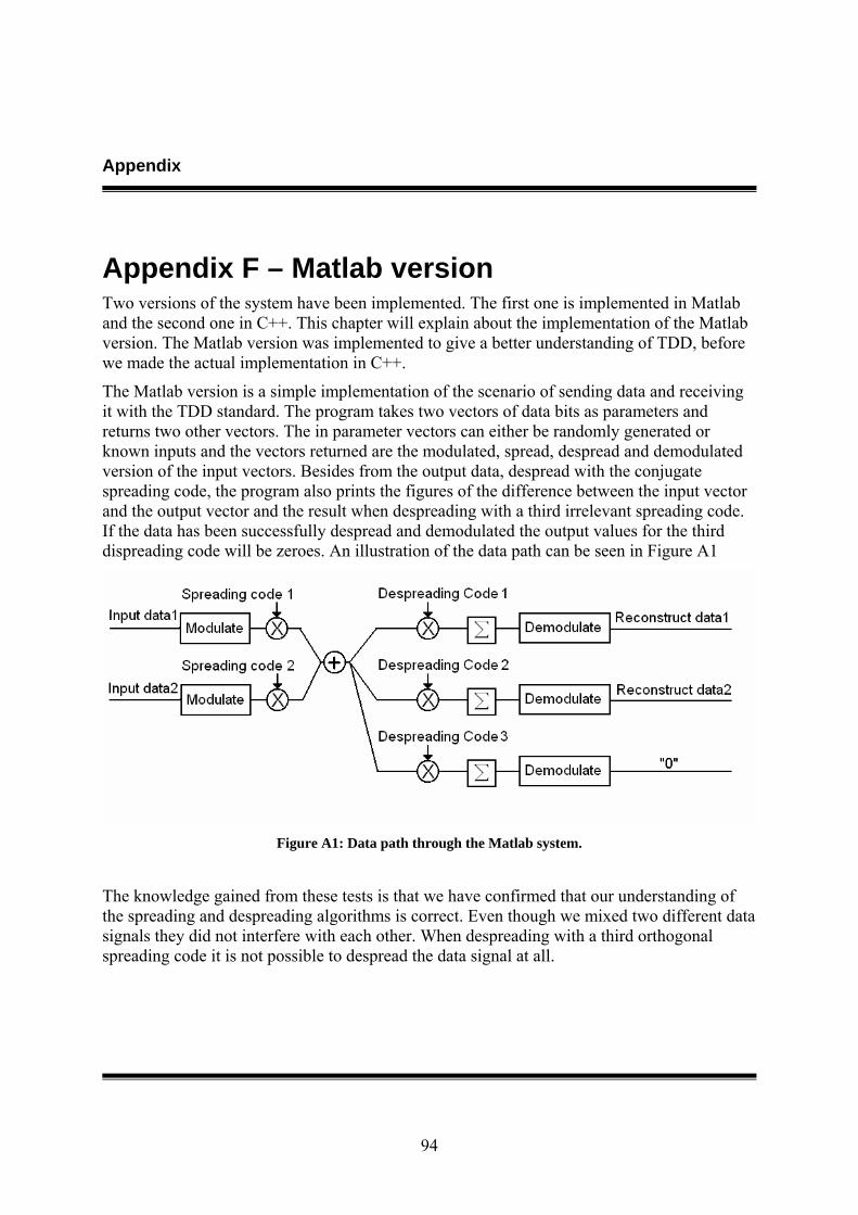
Appendix
94
Appendix F – Matlab version Two versions of the system have been implemented. The first one is implemented in Matlab and the second one in C++. This chapter will explain about the implementation of the Matlab version. The Matlab version was implemented to give a better understanding of TDD, before we made the actual implementation in C++.
The Matlab version is a simple implementation of the scenario of sending data and receiving it with the TDD standard. The program takes two vectors of data bits as parameters and returns two other vectors. The in parameter vectors can either be randomly generated or known inputs and the vectors returned are the modulated, spread, despread and demodulated version of the input vectors. Besides from the output data, despread with the conjugate spreading code, the program also prints the figures of the difference between the input vector and the output vector and the result when despreading with a third irrelevant spreading code. If the data has been successfully despread and demodulated the output values for the third dispreading code will be zeroes. An illustration of the data path can be seen in Figure A1
Figure A1: Data path through the Matlab system.
The knowledge gained from these tests is that we have confirmed that our understanding of the spreading and despreading algorithms is correct. Even though we mixed two different data signals they did not interfere with each other. When despreading with a third orthogonal spreading code it is not possible to despread the data signal at all.
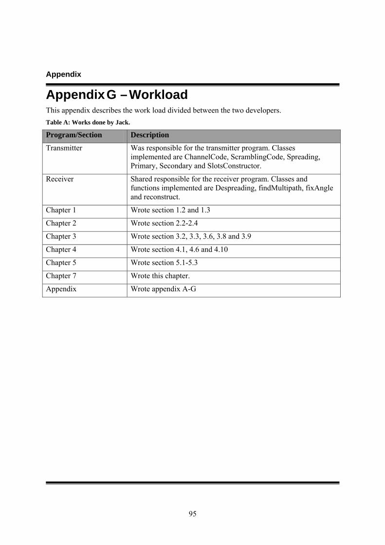
Appendix
95
Appendix G – Workload
This appendix describes the work load divided between the two developers. Table A: Works done by Jack.
Program/Section Description
Transmitter Was responsible for the transmitter program. Classes implemented are ChannelCode, ScramblingCode, Spreading, Primary, Secondary and SlotsConstructor.
Receiver Shared responsible for the receiver program. Classes and functions implemented are Despreading, findMultipath, fixAngle and reconstruct.
Chapter 1 Wrote section 1.2 and 1.3
Chapter 2 Wrote section 2.2-2.4
Chapter 3 Wrote section 3.2, 3.3, 3.6, 3.8 and 3.9
Chapter 4 Wrote section 4.1, 4.6 and 4.10
Chapter 5 Wrote section 5.1-5.3
Chapter 7 Wrote this chapter.
Appendix Wrote appendix A-G
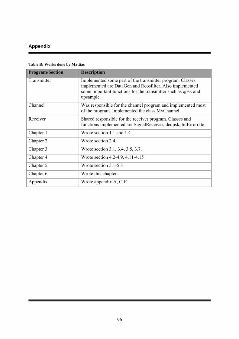
Appendix
96
Table B: Works done by Mattias
Program/Section Description
Transmitter Implemented some part of the transmitter program. Classes implemented are DataGen and Rcosfilter. Also implemented some important functions for the transmitter such as qpsk and upsample.
Channel Was responsible for the channel program and implemented most of the program. Implemented the class MyChannel.
Receiver Shared responsible for the receiver program. Classes and functions implemented are SignalReceiver, deqpsk, bitErrorrate
Chapter 1 Wrote section 1.1 and 1.4
Chapter 2 Wrote section 2.4.
Chapter 3 Wrote section 3.1, 3.4, 3.5, 3.7,
Chapter 4 Wrote section 4.2-4.9, 4.11-4.15
Chapter 5 Wrote section 5.1-5.3
Chapter 6 Wrote this chapter.
Appendix Wrote appendix A, C-E
Appendix
97
På svenska
Detta dokument hålls tillgängligt på Internet – eller dess framtida ersättare – under en längre tid från publiceringsdatum under förutsättning att inga extra-ordinära omständigheter uppstår.
Tillgång till dokumentet innebär tillstånd för var och en att läsa, ladda ner, skriva ut enstaka kopior för enskilt bruk och att använda det oförändrat för ickekommersiell forskning och för undervisning. Överföring av upphovsrätten vid en senare tidpunkt kan inte upphäva detta tillstånd. All annan användning av dokumentet kräver upphovsmannens medgivande. För att garantera äktheten, säkerheten och tillgängligheten finns det lösningar av teknisk och administrativ art.
Upphovsmannens ideella rätt innefattar rätt att bli nämnd som upphovsman i den omfattning som god sed kräver vid användning av dokumentet på ovan beskrivna sätt samt skydd mot att dokumentet ändras eller presenteras i sådan form eller i sådant sammanhang som är kränkande för upphovsmannens litterära eller konstnärliga anseende eller egenart.
För ytterligare information om Linköping University Electronic Press se förlagets hemsida http://www.ep.liu.se/
In English
The publishers will keep this document online on the Internet - or its possible replacement - for a considerable time from the date of publication barring exceptional circumstances.
The online availability of the document implies a permanent permission for anyone to read, to download, to print out single copies for your own use and to use it unchanged for any non-commercial research and educational purpose. Subsequent transfers of copyright cannot revoke this permission. All other uses of the document are conditional on the consent of the copyright owner. The publisher has taken technical and administrative measures to assure authenticity, security and accessibility.
According to intellectual property law the author has the right to be mentioned when his/her work is accessed as described above and to be protected against infringement.
For additional information about the Linköping University Electronic Press and its procedures for publication and for assurance of document integrity, please refer to its WWW home page: http://www.ep.liu.se/
© [Mattias Gylin and Jack Huynh]