Embed Size (px)
Citation preview

Reg. No. 1998/07367/07 ● VAT Reg.No. 4490189489
PostNet Suite #251, Private Bag X1015, Lyttelton, 0140 ● www.investmech.com
Tel +27 12 664-7604 ● Fax +27 86535-1379● Cell: +27 82 445-0510
E-mail address: [email protected]
Behaviour of welded structures under dynamic loading
Weld fatigue course
Prepared for
Universities
DIRECTORS:
M Heyns Pr.Eng., Ph.D., (Managing)
CJ Botha B.Eng(Hons): Industrial
Document No:
Revision:
Date:
IM-TR000
0.0
1 August 2017

Confidential IM-TR000 (Rev 0.0)
Confidential 2
Document information
Project Name: Weld fatigue course
Title: Behaviour of welded structures under dynamic loading
Author: Author
Project Engineer: Dr. Michiel Heyns Pr.Eng.
Document Number: IM-TR000
Filename: Investmech (Behaviour of welded structures under variable amplitude loading) TN R0.0.docx
Creation Date: 22 August 2013
Revision: 0.0
Revision Date: 1 August 2017
Approval
Responsibility Name Designation Signature Date
Not applicable
Distribution list
Name Company / Division Copies
Weld Fatigue Students Universities 1
DCC (Tenders & Quotations) Investmech (Pty) Ltd Original
Summary
This document is the master document for the discussion of the behaviour of welded structures under dynamic loading.

Confidential IM-TR000 (Rev 0.0)
Confidential 3
Software applications The following software applications were used in the execution of this project:
Product Name Version
PC Matlab 2008R1
Microsoft Excel 2010
Microsoft PowerPoint 2010
Microsoft Word 2010
Acrobat 2010
Calculation files The following calculation files were used in the analysis:
Description File Name Revision
Strain life calculation modelling sequence effect of strain
Strain life example - Sequence effect.xls
0.0
Construction of S-N curve PlotSNcurve.m 0.0
Models The following models were used in the analysis:
Model Title Model Number Revision
Not applicable
Input Data Files The following input files are applicable:
Description File Name
Notch effects on welds Investmech - Structural Integrity (Notch effects of welds) R0.0.pptx
Static failure theories Investmech - Structural Integrity (Static Failure Theories) R0.0.pptx
Variable amplitude loading on steel members
Investmech - Structural Integrity (Variable Amplitude Loading) R0.0.pptx
Cycle counting using the rainflow method Investmech - Structural Integrity (Cycle counting) R0.0.pptx
Stress life analysis Investmech - Fatigue (Stress life analysis) R0.0.pptx
Strain life analysis Investmech - Fatigue (Strain life analysis) R0.0.pptx

Confidential IM-TR000 (Rev 0.0)
Confidential 4
Fatigue life improvement techniques for steel and stainless steel
Investmech - Structural Integrity (Fatigue life improvement techniques for steel and stainless steel) R0.0.pptx
Output Data Files The following output files are applicable:
Description File Name
MS Word document with problems done in class as well as notes made in class. This document will be submitted by e-mail to class members after completion of the module
Class notes.docx. The same notes document is used for both days to have all in one document.
MS Excel document with calculations done in class
Class calculations.xlsx. The same Excel document is used for both days to have all in one document.

Confidential IM-TR000 (Rev 0.0)
Confidential 5
Table of Contents
1. INTRODUCTION .......................................................................................................................... 10
2. STUDY MATERIAL ....................................................................................................................... 10
3. TERMINOLOGY ........................................................................................................................... 10
4. BEHAVIOUR OF WELDED STRUCTURES UNDER VARIABLE AMPLITUDE LOADING ......... 13
4.1. Objective .............................................................................................................................. 13
4.2. Scope ................................................................................................................................... 13
4.3. Outcomes ............................................................................................................................. 13
5. FATIGUE S-N CURVES AND DAMAGE ...................................................................................... 15
5.1. Constant amplitude alternating stress parameters .............................................................. 15
5.2. S-N curve for steel ............................................................................................................... 16
5.2.1. Example ....................................................................................................................... 18
5.3. Non-ferrous alloys ................................................................................................................ 18
5.4. Fatigue ratio ......................................................................................................................... 18
5.4.1. Endurance limit and surface hardness ........................................................................ 18
5.4.2. Endurance limit and ultimate tensile strength of steel and cast steel ......................... 18
5.4.3. Other materials ............................................................................................................ 18
5.5. Typical EN 1993-1-9 𝑺𝒓 − 𝑵 curve ...................................................................................... 19
5.5.1. Using the idea .............................................................................................................. 19
5.6. Damage modelling and summing ........................................................................................ 20
5.6.1. Linear damage rule – Palmgren-Miner’s rule_ ............................................................ 20
5.6.2. Shortcomings of the linear damage rule ..................................................................... 20
5.6.3. Summary ..................................................................................................................... 21
6. NOTCH STRESS ASSESSMENT OF WELD DETAIL ................................................................. 22
6.1. Principle of the notch stress approach ................................................................................. 22
6.2. Fictitious notch rounding – effective notch stress approach ................................................ 22
6.2.1. Critical distance approach ........................................................................................... 23
6.3. Simple design S-N curve according to IIW Bulletin 520 ...................................................... 24
6.4. Design S-N curve ................................................................................................................. 24
6.5. Applied to a cruciform joint ................................................................................................... 24
6.6. References ........................................................................................................................... 26
7. STATIC FAILURE THEORIES ..................................................................................................... 27
7.1. Principal stress ..................................................................................................................... 27
7.2. Principal axes ....................................................................................................................... 28
7.3. Failure theories .................................................................................................................... 28
7.3.1. Maximum normal stress .............................................................................................. 28
7.3.2. Maximum shear stress ................................................................................................ 29
7.3.3. Von Mises failure theory .............................................................................................. 29
7.3.4. Octahedral shear stress theory ................................................................................... 30
7.3.5. Mohr’s failure theory .................................................................................................... 30
7.3.6. These are not all .......................................................................................................... 30
7.3.7. Which static theory can be used ................................................................................. 30
7.4. Buckling ................................................................................................................................ 31
7.5. Non stress-based criteria ..................................................................................................... 31
7.6. Conclusion ........................................................................................................................... 31
8. VARIABLE AMPLITUDE LOADING ............................................................................................. 31
8.1. Types of loading ................................................................................................................... 32
Confidential IM-TR000 (Rev 0.0)
Confidential 6
8.2. Causes for loads on structures ............................................................................................ 32
8.3. Loads and stress-strain ........................................................................................................ 32
8.4. Classification of signal types ................................................................................................ 33
8.5. Statistical parameters ........................................................................................................... 33
8.5.1. Peak value ................................................................................................................... 33
8.5.2. Peak-to-peak value...................................................................................................... 33
8.5.3. Mean ............................................................................................................................ 33
8.5.1. Root-mean-square ....................................................................................................... 34
8.5.2. Crest factor .................................................................................................................. 34
8.5.3. Variance and standard deviation ................................................................................. 34
8.5.4. Kurtosis ........................................................................................................................ 34
8.5.5. Example ....................................................................................................................... 34
8.6. Presentation of stress data .................................................................................................. 35
8.7. Stress histories ..................................................................................................................... 35
8.8. Obtaining stress spectra for fatigue calculations ................................................................. 36
8.9. Exceedence diagrams .......................................................................................................... 36
8.9.1. Errors and effects ........................................................................................................ 37
8.10. Variable amplitude loading ................................................................................................... 38
8.11. Cycle counting methods – discussed ................................................................................... 38
8.11.1. Level crossing .............................................................................................................. 38
8.11.2. Peak counting .............................................................................................................. 39
8.11.3. Simple-range counting ................................................................................................ 40
8.11.4. Rainflow counting ........................................................................................................ 41
8.11.5. Sequence effects ......................................................................................................... 42
8.11.6. More info on Rainflow counting ................................................................................... 42
8.12. Crack growth retardation using load sequence effects ........................................................ 43
8.12.1. Crack growth retardation prediction methods ............................................................. 45
8.12.2. Further reading ............................................................................................................ 45
8.13. Block loading ........................................................................................................................ 45
8.14. Cumulative damage test program ........................................................................................ 46
8.15. Conclusion ........................................................................................................................... 47
9. CYCLE COUNTING WITH THE RAINFLOW METHOD .............................................................. 47
10. STRESS LIFE ANALYSIS ........................................................................................................ 49
10.1. Slides not in notes ................................................................................................................ 49
10.2. Notches ................................................................................................................................ 50
10.2.1. Weld toes ..................................................................................................................... 50
10.3. Theoretic stress concentration factor ................................................................................... 50
10.4. Notch fatigue factor .............................................................................................................. 51
10.4.1. Notch fatigue factor at 1 000 cycles ............................................................................ 54
10.5. Mean stress correction ......................................................................................................... 54
10.6. Modifying factors .................................................................................................................. 55
10.6.1. Size factor on different shaft sizes .............................................................................. 55
10.6.2. Loading effects ............................................................................................................ 56
10.6.3. Surface finish and corrosion ........................................................................................ 56
10.6.4. Temperature ................................................................................................................ 57
10.6.5. Reliability ..................................................................................................................... 58
10.6.6. Mechanical modifying factors ...................................................................................... 58

Confidential IM-TR000 (Rev 0.0)
Confidential 7
10.7. Derivation of S-N curve for S1000 and Se modified by the fatigue notch factors ................... 59
10.8. Endurance calculation example ........................................................................................... 59
10.9. Fatigue life example with mean stress ................................................................................. 61
10.10. Conclusion ....................................................................................................................... 62
11. STRAIN LIFE ANALYSIS ......................................................................................................... 63
List of Tables Table 1: Characteristic fatigue strength for welds of different materials based on effective notch stress
with 𝒓𝒓𝒆𝒇 = 𝟏 𝒎𝒎 (maximum principal stress)............................................................................. 24
Table 2: Shaft diameter dependent size factor..................................................................................... 56
Table 3: Example fatigue calculation .................................................................................................... 60
List of Figures Figure 1: An example of a constant amplitude alternating stress signal .............................................. 15
Figure 2: Completely reversed S-N curve for structural steel with yield strength 300 MPa for a confidence level of 70% of 50% probability of survival for N ......................................................... 17
Figure 3: Typical EN 1993-1-9 𝑺𝒓 − 𝑵 curve for characteristic strength 𝚫𝝈𝑪 = 𝟏𝟎𝟎 𝑴𝑷𝒂 .................. 19
Figure 4: Linear cumulative damage - Palmgren-Miner's rule on an 𝑺𝒓 − 𝑵 curve ............................. 20
Figure 5: Notch stress application ........................................................................................................ 23
Figure 6: Substitute micro-structural length .......................................................................................... 23
Figure 7: Comparison of failure theories .............................................................................................. 29
Figure 8: Level-crossing counting ........................................................................................................ 39
Figure 9: Peak-counting ........................................................................................................................ 40
Figure 10: Simple-range counting ........................................................................................................ 40
Figure 11: Load sequence effects ........................................................................................................ 42
Figure 12: Crack growth retardation due to overloading ...................................................................... 43
Figure 13: Crack growth retardation of a structural steel ..................................................................... 44
Figure 14: Crack-tip plasticity ............................................................................................................... 45
Figure 15: Stress concentrations at weld toes result in crack initiation ................................................ 50
Figure 16: Stress concentration factors for various geometries and modes of loading ....................... 51
Figure 17: S-N curve adjusted for a notched material .......................................................................... 52
Figure 18: Finite element analysis of a plate with a hole in the middle ................................................ 53
Figure 19: Stress concentration factors for a plate with a hole in the middle ....................................... 53
Figure 20: Ration between notch fatigue factors at 1 000 and 1M cycles vs tensile strength ............. 54
Figure 21: Haigh diagram sketch showing the regions for finite and infinite life .................................. 55
Figure 22: Haigh diagram for AISI 4340 steel (Bannantine et all, 1990:7) ........................................... 55
Figure 23: Surface finish modification factors for steel (ASM International, 2008:16) ......................... 57
Figure 24: Relationship between fatigue notch factors at endurance and 1000 cycles ....................... 61

Confidential IM-TR000 (Rev 0.0)
Confidential 8
List of symbols and abbreviations
𝑘1 Magnification factor for nominal stress ranges to account for secondary bending moments in
trusses
𝑘𝑓 Stress concentration factor
𝑘𝑠 Reduction factor for fatigue stress to account for size effects
𝑚 Slope of the fatigue curve
𝑚1 Slope of the fatigue curve for stress range above the constant amplitude fatigue limit
𝑚2 Slope of the fatigue curve for stress ranges between the cut-off limit and constant amplitude
fatigue limit
𝑁𝑅 Design life time expressed as number of cycles related to a constant stress range.
𝑄𝑘 Characteristic value of a single action [N]
Greek symbols:
𝛽 Geometric stress concentration factor
𝛾𝐹𝑓 Partial factor for equivalent constant amplitude stress ranges Δ𝜎𝐸 , Δ𝜏𝐸
𝛾𝑀𝑓 Partial factor for fatigue strength Δ𝜎𝐶 , Δ𝜏𝐶
𝜀 Strain. If there is a subscript it indicates the direction of the strain. For example, 𝜀𝑥 is
strain in the x-direction.
𝜂 Eta
𝜃 Angle [°]
𝜆𝑖 Damage equivalent factors
𝜈 Poisson ratio
Δ𝜎 Direct stress range [Pa]
Δ𝜏 Shear stress range [Pa]
Δ𝜎𝑒𝑞 Equivalent stress range for connections in webs of orthotropic decks [Pa]
Δ𝜎𝐶 , Δ𝜏𝐶 Reference value of the fatigue strength at 𝑁𝐶 = 2×10⁶ cycles [Pa]
Δ𝜎𝐷, Δ𝜏𝐷 Fatigue limit for constant amplitude stress range at 𝑁𝐷 cycles [Pa]
Δ𝜎𝐸 , Δ𝜏𝐸 Equivalent constant amplitude stress range related to 𝑛𝑚𝑎𝑥 [Pa]
Δ𝜎𝐸2, Δ𝜏𝐸2 Equivalent constant amplitude stress range related to 2 million cycles [Pa]
Δ𝜎𝐿, Δ𝜏𝐿 Cut-off limit for stress ranges at 𝑁𝐿 cycles [Pa]
Δ𝜎𝐶,𝑟𝑒𝑑 Reduced reference value of the fatigue strength [Pa]
Note, the lists above do not contain symbols that are clearly defined in the section or that are indicated on sketches.
Confidential IM-TR000 (Rev 0.0)
Confidential 9
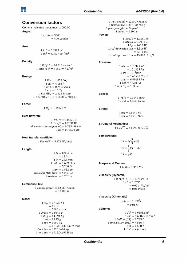
Conversion factors Comma indicates thousands: 1,000.00
Angle:
1 𝑐𝑖𝑟𝑐𝑙𝑒 = 360 ° = 400 𝑔𝑟𝑎𝑑𝑒𝑠
Area:
1 𝑓𝑡2 = 0.0929 𝑚2 1 𝑖𝑛2 = 6.452×10⁻⁴𝑚2
Density:
1 𝑙𝑏 𝑓𝑡3⁄ = 16.018 𝑘𝑔 𝑚3⁄ 1 𝑠𝑙𝑢𝑔 𝑓𝑡3⁄ = 515.379 𝑘𝑔 𝑚3⁄
Energy:
1 𝐵𝑡𝑢 = 1,055.06 𝐽 1 𝑐𝑎𝑙 = 4.186 𝐽
1 ℎ𝑝 ℎ = 0.7457 𝑘𝑊ℎ 1 𝑒𝑟𝑔 = 10−7𝐽
1 𝐵𝑡𝑢 𝑙𝑏𝑚⁄ = 2.326 𝑘𝐽 𝑘𝑔⁄ 1 𝐵𝑡𝑢 (𝑙𝑏𝑚°𝐹)⁄ = 4.1868 𝑘𝐽 (𝑘𝑔𝐾)⁄
Force:
1 𝑙𝑏𝑓 = 4.44822 𝑁
Heat flow rate:
1 𝐵𝑡𝑢 𝑠⁄ = 1,055.1 𝑊 1 𝐵𝑡𝑢 ℎ⁄ = 0.2931 𝑊
1 ℎ𝑘 (𝑚𝑒𝑡𝑟𝑖𝑐 ℎ𝑜𝑟𝑠𝑒 𝑝𝑜𝑤𝑒𝑟) = 0.735499 𝑘𝑊 1 ℎ𝑝 = 0.74570 𝑘𝑊
Heat transfer coefficient:
1 𝐵𝑡𝑢 ℎ°𝐹⁄ = 5.678 𝑊 𝑚2𝐾⁄
Length:
1 𝑓𝑡 = 0.3048 𝑚 = 12 𝑖𝑛
1 𝑖𝑛 = 25.4 𝑚𝑚 1 𝑚𝑖𝑙𝑒 = 1.6093 𝑘𝑚
= 5,280 𝑓𝑡 1 𝑛𝑚 = 1.852 𝑘𝑚
𝑁𝑎𝑢𝑡𝑖𝑐𝑎𝑙 𝑀𝑖𝑙𝑒 (𝑛𝑚) = 𝑆𝑒𝑎 𝑀𝑖𝑙𝑒 𝐴𝑛𝑔𝑠𝑡𝑟𝑜𝑚 = 10−10 𝑚
Luminous Flux:
1 𝑐𝑎𝑛𝑑𝑙𝑒 𝑝𝑜𝑤𝑒𝑟 = 12.566 𝑙𝑢𝑚𝑒𝑛 = 0.0188 𝑊
Mass:
1 𝑙𝑏𝑚 = 0.4536 𝑘𝑔 = 16 𝑜𝑧 = 7000 𝑔𝑟𝑎𝑖𝑛
1 𝑔𝑟𝑎𝑖𝑛 = 0.0648 𝑔 1 𝑠𝑙𝑢𝑔 = 14.594 𝑘𝑔
1 𝑜𝑧 = 28.35 𝑔 1 𝑡𝑜𝑛 = 1000 𝑘𝑔
= 1.10231131 𝑠ℎ𝑜𝑟𝑡 𝑡𝑜𝑛𝑠 1 𝑠ℎ𝑜𝑟𝑡 𝑡𝑜𝑛 = 907.18474 𝑘𝑔 1 𝑙𝑜𝑛𝑔 𝑡𝑜𝑛 = 1016.0469088 𝑘𝑔
1 𝑡𝑟𝑜𝑦 𝑝𝑜𝑢𝑛𝑑 = 12 𝑡𝑟𝑜𝑦 𝑜𝑢𝑛𝑐𝑒𝑠 1 𝑡𝑟𝑜𝑦 𝑜𝑢𝑛𝑐𝑒 = 31.1034768 𝑔
1 𝑝𝑒𝑛𝑛𝑦𝑤𝑒𝑖𝑔ℎ𝑡 = 24 𝑔𝑟𝑎𝑖𝑛 1 𝑐𝑎𝑟𝑎𝑡 = 0.200 𝑔
Power:
1 𝐵𝑡𝑢 𝑠⁄ = 1,055.1 𝑊 1 𝐵𝑡𝑢 ℎ⁄ = 0.2931 𝑊
1 ℎ𝑝 = 745.7 𝑊 1 𝑟𝑒𝑓𝑟𝑖𝑔𝑒𝑟𝑎𝑡𝑖𝑜𝑛 𝑡𝑜𝑛 = 3,516 𝑊
= 3.516 𝑘𝑊 1 𝑐𝑜𝑜𝑙𝑖𝑛𝑔 𝑡𝑜𝑤𝑒𝑟 𝑡𝑜𝑛 = 15,000 𝐵𝑡𝑢 ℎ⁄
Pressure:
1 𝑎𝑡𝑚 = 101.325 𝑘𝑃𝑎 = 101,325 𝑃𝑎
1 𝑃𝑎 = 10−5𝐵𝑎𝑟 = 1.45×10⁻⁴ 𝑝𝑠𝑖
1 𝑝𝑠𝑖 = 6.8948 𝑘𝑃𝑎 1 𝑝𝑠𝑓 = 47.88 𝑃𝑎
1 𝑚𝑚 𝐻𝑔 = 133 𝑃𝑎
Speed:
1 𝑓𝑡 𝑠⁄ = 0.3048 𝑚 𝑠⁄ 1 𝑘𝑛𝑜𝑡 = 1.852 𝑘𝑚 ℎ⁄
Stress:
1 𝑝𝑠𝑖 = 6,8948 𝑃𝑎 1 𝑘𝑠𝑖 = 6.8948 𝑀𝑃𝑎
Structural Mechanics:
1 𝑘𝑠𝑖√𝑖𝑛 = 1.0792 𝑀𝑃𝑎√𝑚
Temperature:
°𝐹 = °𝐶9
5+ 32
°𝐶 =5
9[°𝐹 − 32]
°𝑅 =5
9𝐾
Torque and Moment:
1 𝑓𝑡 𝑙𝑏 = 1.356 𝑁𝑚
Viscosity (Dynamic)
1 𝑙𝑏 (𝑓𝑡 ∙ 𝑠)⁄ = 1.4879 𝑃𝑎 ∙ 𝑠 1 𝑐𝑃 = 10−3𝑃𝑎 ∙ 𝑠
= 0.001 𝑁𝑠 𝑚2⁄ = 0.01 𝑃𝑜𝑖𝑠𝑒
Viscosity (Kinematic)
1 𝑐𝑆𝑡 = 10−6 𝑚2
𝑠⁄ = 0.01 𝑆𝑡
Volume:
1 𝑓𝑡3 = 0.02832 𝑚3 1 𝑖𝑛3 = 1.6387×10⁻⁵𝑚3
1 𝐺𝑎𝑙𝑙𝑜𝑛 (𝑈𝑆) = 3.785 ℓ 1 𝐼𝑚𝑝. 𝐺𝑎𝑙𝑙𝑜𝑛 (𝑈𝐾) = 4.546 ℓ
1 𝑝𝑡 = 0.568 ℓ 1 𝑑𝑚3 = ℓ (𝐿𝑖𝑡𝑒𝑟)

Confidential IM-TR000 (Rev 0.0)
Confidential 10
1. INTRODUCTION
This document presents the class notes to understand the behaviour of welded structures under dynamic loading. This section introduces concepts to students whereas the following Module 3.8 focuses on the design of welded structures under dynamic loading. Therefore, this section is more information and introduces basic principles. Module 3.8 introduces application of the concepts by calculation.
2. STUDY MATERIAL
The student shall arrange access to the following documents:
1. Slides presented in class.
2. This guide.
3. TERMINOLOGY
This section summarises terminology used in the lectures and come from BS EN 1993-1-9 (2005:7:9):
Fatigue
The process of initiation and propagation of cracks through a structural part or member due to the action of fluctuating stress.
Nominal stress
A stress in the parent material or in a weld adjacent to a potential crack location calculated in accordance with elastic theory excluding all stress concentration effects.j The nominal stress can be a direct stress, shear stress, principal stress or equivalent stress.
Modified nominal stress
A nominal stress multiplied by an appropriate stress concentration factor 𝑘𝑓 to allow for a geometric
discontinuity that has not been taken into account in the classification of a particular constructional detail.
Geometric stress = hot spot stress
The maximum principal stress in the parent material adjacent to the weld toe, taking into account stress concentration effects due to the overall geometry of a particular constructional detail. Local stress concentration effects e.g. from the weld profile shape (which is already included in the detail categories in Appendix B of BS EN 1993-1-9 for the geometric stress method)) need not to be considered.
Residual stress
Residual stress is a permanent state of stress in a structure that is in equilibrium and is independent of the applied actions. Residual stresses can arise from rolling stresses, cutting processes, welding shrinkage or lack of fit between members or from any loading event that causes yielding of part of the structure.
Loading event
A defined loading sequence applied to the structure and giving rise to a stress history, which is normally repeated a defined number of times in the life of the structure.
Stress history
A record or a calculation of the stress variation at a particular point in a structure during a loading event.

Confidential IM-TR000 (Rev 0.0)
Confidential Page 11 of 63
Rainflow method
Particular cycle counting method of producing a stress-range spectrum from a given stress history.
Reservoir method
Particular cycle counting method of producing a stress-range spectrum from a given stress history.
Stress range
Algebraic difference between the two extremes of a particular stress cycle derived from a stress history.
Stress-range spectrum
Histogram of the number of occurrences for all stress ranges of different magnitudes recorded or calculated for a particular loading event.
Design spectrum
The total of all stress-range spectra in the design life of a structure relevant to the fatigue assessment.
Design life
The reference period of time for which a structure is required to perform safely with an acceptable probability that failure by fatigue cracking will occur.
Fatigue life
The predicted period of time to cause fatigue failure under the application of the design spectrum.
Miner’s summation
A linear cumulative damage calculation based on the Palmgren-Miner rule.
Equivalent constant amplitude stress range
The constant amplitude stress range that would result in the same fatigue life as for the design spectrum, when the comparison is based on a Miner’s summation.
Fatigue loading
A set of action parameters based on typical loading events described by the positions of loads, their magnitudes, frequencies of occurrence, sequence and relative phasing.
Equivalent constant amplitude fatigue loading
Simplified constant amplitude loading causing the same fatigue damage effects as a series of actual variable amplitude loading events.
Fatigue strength curve
The quantitative relationships between the stress range and number of stress cycles to fatigue failure, used for the fatigue assessment of a particular category of structural detail. The fatigue strengths given in BS EN 1993-1-9 are lower bound values based on the evaluation of fatigue tests with large scale test specimens in accordance with EN 1990 – Annex D.
Detail category
The numerical designation given to a particular detail for a given direction of stress fluctuation, in order to indicate which fatigue strength curve is applicable for the fatigue assessment (The detail category number indicates the reference fatigue strength Δ𝜎𝐶 in MPa).

Confidential IM-TR000 (Rev 0.0)
Confidential Page 12 of 63
Constant amplitude fatigue limit
The limiting direct or shear stress range value below which no fatigue damage will occur in tests under constant amplitude stress conditions. Under variable amplitude conditions all stress range have to be below this limit for no fatigue damage to occur.
Cut-off limit
The limit below which stress ranges of the design spectrum do not contribute to the calculated cumulative damage.
Endurance
The life to failure expressed in cycles, under the action of a constant amplitude stress history.
Reference fatigue strength
The constant amplitude stress range Δ𝜎𝐶 for a particular detail category for an endurance of 𝑁 =1×10⁶ cycles

Confidential IM-TR000 (Rev 0.0)
Confidential Page 13 of 63
4. BEHAVIOUR OF WELDED STRUCTURES UNDER VARIABLE AMPLITUDE LOADING
4.1. Objective
Understand in detail:
1. The development of fatigue
2. Calculation of load cycles
3. Influence of notches and their avoidance
4.2. Scope
The following material will be covered:
1. Types and variables of cyclic loading
2. Statistical stress analysis on real structures
3. S-N diagrams
4. Stress collective
5. Fatigue strength
6. Effect of mean stress including residual stresses
7. Effect of stress range
8. Stress distribution
9. Influence of notches
10. Influence of weld imperfections
11. Weld fatigue improvement techniques
a. Surface protection
b. Needle peening
c. TIG dressing
d. Burr grinding
e. Hammering
f. Stress relieving
12. Standards, ISO, CEN and National
13. Palmgren-Miner rule
14. Classification of weld joints
4.3. Outcomes
After completion of this section you will be able to:
1. Draw and interpret an S-N diagram.
2. Explain fully the methods of counting load cycles.
3. Calculate the stress ratio.
4. Detail the influence of notches and weld defects.
5. Explain fully the methods for improving fatigue performance.
Confidential IM-TR000 (Rev 0.0)
Confidential 14
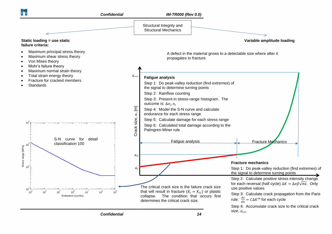
Structural Integrity and Structural Mechanics
Static loading = use static failure criteria:
Variable amplitude loading
• Maximum principal stress theory
• Maximum shear stress theory
• Von Mises theory
• Mohr’s failure theory
• Maximum normal strain theory
• Total strain energy theory
• Fracture for cracked members
• Standards
A defect in the material grows to a detectable size where after it propagates to fracture.
Cra
ck s
ize
, 𝑎
, [m
]
Fatigue analysis Fracture Mechanics
Fatigue analysis
Step 1: Do peak-valley reduction (find extremes) of the signal to determine turning points
Step 2: Rainflow counting
Step 3: Present in stress-range histogram. The outcome is: Δ𝜎𝑖 , 𝑛𝑖
Step 4: Model the S-N curve and calculate endurance for each stress range
Step 5: Calculate damage for each stress range
Step 6: Calculated total damage according to the Palmgren-Miner rule
𝑎𝑖
𝑎𝑑
𝑎𝑐𝑟𝑖
Fracture mechanics
Step 1: Do peak-valley reduction (find extremes) of the signal to determine turning points
Step 2: Calculate positive stress intensity change
for each reversal (half cycle) Δ𝐾 = Δ𝜎𝛽√𝜋𝑎. Only use positive values
Step 3: Calculate crack propagation from the Paris
rule: 𝑑𝑎
𝑑𝑁= 𝐶Δ𝐾𝑚 for each cycle
Step 4: Accumulate crack size to the critical crack size, 𝑎𝑐𝑟𝑖
The critical crack size is the failure crack size that will result in fracture (𝐾𝐼 = 𝐾𝐼𝐶) or plastic collapse. The condition that occurs first determines the critical crack size.
103
104
105
106
107
108
109
101
102
103
104
Endurance [cycles]
Str
ess r
ange [
MP
a]
S-N curve for detail classification 100
Confidential IM-TR000 (Rev 0.0)
Confidential 15
5. FATIGUE S-N CURVES AND DAMAGE
The objective of this section is to introduce S-N fatigue curves to the student, and enable the student to carry out fatigue calculations for constant amplitude loads.
Presentation used in class: S-N curves and damage
Filename: Investmech – Fatigue (S-N curves and damage) R0.0
5.1. Constant amplitude alternating stress parameters
The purpose of this section is to evaluate the behaviour of weld detail under cyclic loading. The theory of BS EN 1993-1-9 and IIW Bulletin 520 will be applied.
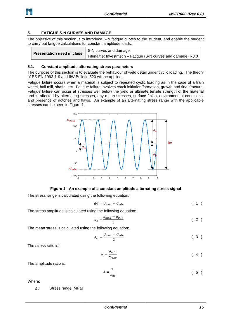
Fatigue failure occurs when a material is subject to repeated cyclic loading as in the case of a train wheel, ball mill, shafts, etc. Fatigue failure involves crack initiation/formation, growth and final fracture. Fatigue failure can occur at stresses well below the yield or ultimate tensile strength of the material and is affected by alternating stresses, any mean stresses, surface finish, environmental conditions, and presence of notches and flaws. An example of an alternating stress range with the applicable stresses can be seen in Figure 1.
Figure 1: An example of a constant amplitude alternating stress signal
The stress range is calculated using the following equation:
∆𝜎 = 𝜎𝑚𝑎𝑥 − 𝜎𝑚𝑖𝑛 ( 1 )
The stress amplitude is calculated using the following equation:
𝜎𝑎 =𝜎𝑚𝑎𝑥 − 𝜎𝑚𝑖𝑛
2 ( 2 )
The mean stress is calculated using the following equation:
𝜎𝑚 =𝜎𝑚𝑎𝑥 + 𝜎𝑚𝑖𝑛
2 ( 3 )
The stress ratio is:
𝑅 =𝜎𝑚𝑖𝑛
𝜎𝑚𝑎𝑥
( 4 )
The amplitude ratio is:
𝐴 =𝜎𝑎
𝜎𝑚 ( 5 )
Where:
∆𝜎 Stress range [MPa]
Δ𝜎
𝜎𝑎
𝜎𝑎
𝜎𝑚𝑖𝑛
𝜎𝑚𝑎𝑥
𝜎𝑚
Confidential IM-TR000 (Rev 0.0)
Confidential Page 16 of 63
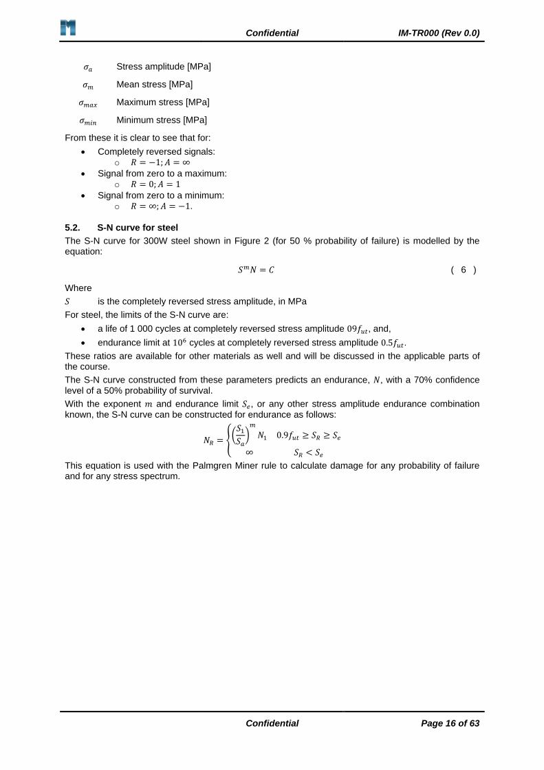
𝜎𝑎 Stress amplitude [MPa]
𝜎𝑚 Mean stress [MPa]
𝜎𝑚𝑎𝑥 Maximum stress [MPa]
𝜎𝑚𝑖𝑛 Minimum stress [MPa]
From these it is clear to see that for:
• Completely reversed signals: o 𝑅 = −1; 𝐴 = ∞
• Signal from zero to a maximum: o 𝑅 = 0; 𝐴 = 1
• Signal from zero to a minimum: o 𝑅 = ∞; 𝐴 = −1.
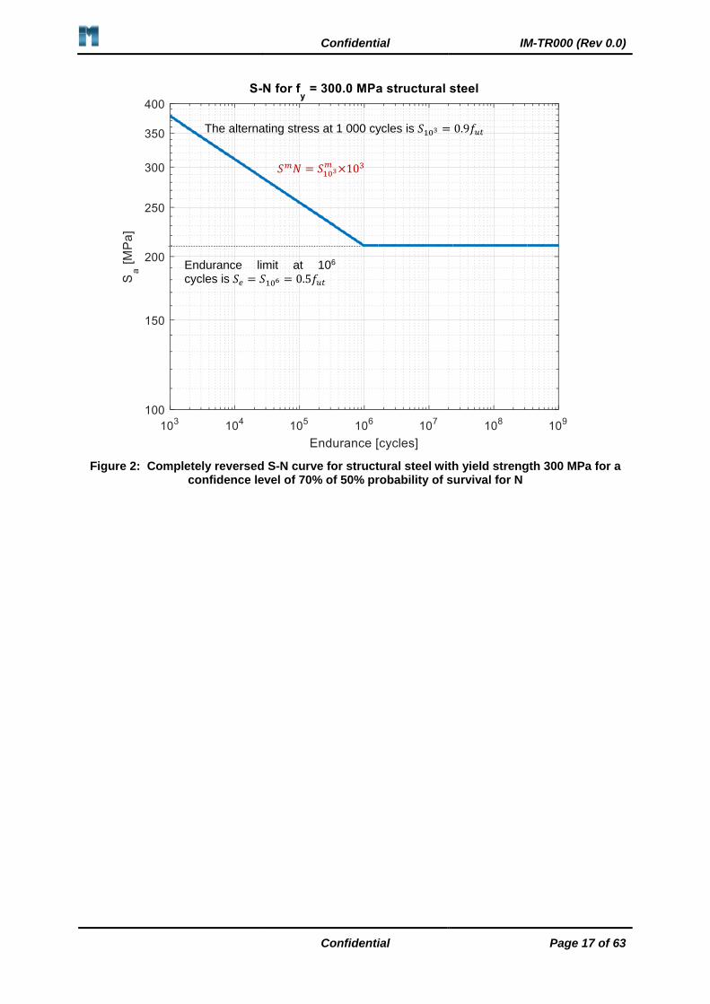
5.2. S-N curve for steel
The S-N curve for 300W steel shown in Figure 2 (for 50 % probability of failure) is modelled by the equation:
𝑆𝑚𝑁 = 𝐶 ( 6 )
Where
𝑆 is the completely reversed stress amplitude, in MPa
For steel, the limits of the S-N curve are:
• a life of 1 000 cycles at completely reversed stress amplitude 09𝑓𝑢𝑡, and,
• endurance limit at 106 cycles at completely reversed stress amplitude 0.5𝑓𝑢𝑡.
These ratios are available for other materials as well and will be discussed in the applicable parts of the course.
The S-N curve constructed from these parameters predicts an endurance, 𝑁, with a 70% confidence level of a 50% probability of survival.
With the exponent 𝑚 and endurance limit 𝑆𝑒, or any other stress amplitude endurance combination known, the S-N curve can be constructed for endurance as follows:
𝑁𝑅 = {(
𝑆1
𝑆𝑎)
𝑚
𝑁1 0.9𝑓𝑢𝑡 ≥ 𝑆𝑅 ≥ 𝑆𝑒
∞ 𝑆𝑅 < 𝑆𝑒
This equation is used with the Palmgren Miner rule to calculate damage for any probability of failure and for any stress spectrum.
Confidential IM-TR000 (Rev 0.0)
Confidential Page 17 of 63
Figure 2: Completely reversed S-N curve for structural steel with yield strength 300 MPa for a confidence level of 70% of 50% probability of survival for N
The alternating stress at 1 000 cycles is 𝑆103 = 0.9𝑓𝑢𝑡
Endurance limit at 106 cycles is 𝑆𝑒 = 𝑆106 = 0.5𝑓𝑢𝑡
𝑆𝑚𝑁 = 𝑆103𝑚 ×103
Confidential IM-TR000 (Rev 0.0)
Confidential Page 18 of 63
5.2.1. Example
Construct the S-N curve for a material with completely reversed stress amplitude 𝑆1 = 500 𝑀𝑃𝑎 at
𝑁1 = 103 and endurance limit 𝑆𝑒 = 150 𝑀𝑃𝑎 at 𝑁𝑒 = 106 cycles.
Solution
Two points are given on the S-N curve, for which the following equation applies:
𝑆1𝑚𝑁1 = 𝑆2
𝑚𝑁2 ( 7 )
The exponent, 𝑚, can be calculated as follows:
(𝑆1
𝑆2)
𝑚
=𝑁2
𝑁1
𝑚 log (𝑆1
𝑆2) = log (
𝑁2
𝑁1)
𝑚 =log (
𝑁2
𝑁1)
log (𝑆1
𝑆2)
= 5.74
( 8 )
Now, the endurance, 𝑁𝑅 at any completely reversed stress amplitude, 𝑆𝑎 is as follows
𝑁𝑅 = {(
𝑆1
𝑆𝑎)
𝑚
𝑁1 0.9𝑓𝑢𝑡 ≥ 𝑆𝑅 ≥ 𝑆𝑒
∞ 𝑆𝑅 < 𝑆𝑒
( 9 )
5.3. Non-ferrous alloys
The pseudo-endurance limit is specified as the stress value at 500 million cycles.
5.4. Fatigue ratio
The fatigue ratio is the ratio of endurance limit to ultimate tensile strength:
𝑓𝑟 =𝑆𝑒
𝑓𝑢𝑡
For steel 𝑓𝑟 varies between 0.35 and 0.6. Most steels with 𝑓𝑢𝑡 < 1 400 𝑀𝑃𝑎 have a fatigue ratio of 0.5.
5.4.1. Endurance limit and surface hardness
As function of surface hardness of material:
𝑆𝑒 = {0.25𝐵𝐻𝑁 𝑘𝑠𝑖 𝑓𝑜𝑟 𝐵𝐻𝑁 ≤ 400
100 𝑘𝑠𝑖 𝑓𝑜𝑟 𝐵𝐻𝑁 > 400
5.4.2. Endurance limit and ultimate tensile strength of steel and cast steel
In terms of ultimate tensile strength:
Steel
𝑆𝑒 = {0.5𝑆𝑢𝑡 𝑓𝑜𝑟 𝑆𝑢𝑡 ≤ 200 𝑘𝑠𝑖 (1 400 𝑀𝑃𝑎)
100 𝑘𝑠𝑖 (700 𝑀𝑃𝑎) 𝑓𝑜𝑟 𝑆𝑢𝑡 > 200 𝑘𝑠𝑖 (1 400 𝑀𝑃𝑎)
Cast Iron + Cast Steels:
𝑆𝑒 = {0.45𝑆𝑢𝑡 𝑓𝑜𝑟 𝑆𝑢𝑡 ≤ 600 𝑀𝑃𝑎
275 𝑀𝑃𝑎 𝑓𝑜𝑟 𝑆𝑢𝑡 > 600 𝑀𝑃𝑎
5.4.3. Other materials
Deriving constants for other materials:
• Not so simple because of potential non-linear S-N characteristics
• Linear approximation used in most applications due to empirical data used in analysis – statistical errors exists already
Confidential IM-TR000 (Rev 0.0)
Confidential Page 19 of 63
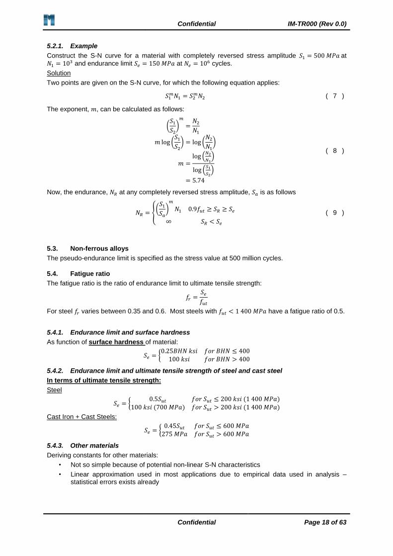
5.5. Typical EN 1993-1-9 𝑺𝒓 − 𝑵 curve
The fatigue curves used in EN 1993-1-9 standard has the form shown in Figure 3. Please populate the curve with information supplied in the slides.
Figure 3: Typical EN 1993-1-9 𝑺𝒓 − 𝑵 curve for characteristic strength 𝚫𝝈𝑪 = 𝟏𝟎𝟎 𝑴𝑷𝒂
5.5.1. Using the idea
Calculate the constant amplitude fatigue limit and the cut-off limit for a detail category 100, i.e., the characteristic strength is Δ𝜎𝐶 = 100 MPa.
Solution
Make your own notes from information supplied in class.
Confidential IM-TR000 (Rev 0.0)
Confidential Page 20 of 63
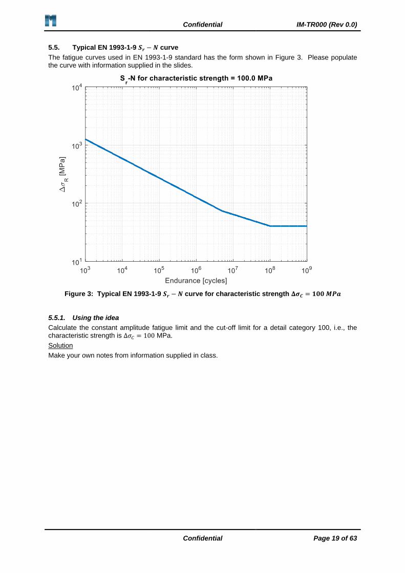
5.6. Damage modelling and summing
5.6.1. Linear damage rule – Palmgren-Miner’s rule_
The linear Palmgren-Miner’s damage rule states that the damage due to a stress amplitude is equal to the number of cycles that the stress amplitude is applied divided by the endurance (number of cycles to crack initiation) at that stress amplitude.
𝐷𝑖 =𝑛𝑖
𝑁𝑖 ( 10 )
If there are more than one stress amplitude applied to the component, then the total damage is the sum of the damages due to the individual stress conditions, as shown in Figure 4.
𝐷𝑇 = ∑𝑛𝑖
𝑁𝑖
𝑘
𝑖=1 ( 11 )
Test results showed that crack initiation occurs when the total damage range between 0.5 and 2.0. For calculation purposes, failure will be assumed when 𝐷𝑇 = 1.0.
0.5 ≤ 𝐷𝑇 ≤ 2.0
Figure 4: Linear cumulative damage - Palmgren-Miner's rule on an 𝑺𝒓 − 𝑵 curve
5.6.2. Shortcomings of the linear damage rule
• It does not consider sequence effects
• It is amplitude independent
• Predicts that the rate of damage accumulation is independent of stress level. Observed behaviour show that at high strain amplitudes cracks will initiate in a few cycles, whereas at low strain amplitudes almost all of the life is spent initiating a crack.
Non-linear damage theories
– Practical problems
Δ𝜎1
Δ𝜎2
Δ𝜎𝑘
𝑁1 𝑁2 𝑁𝑘

Confidential IM-TR000 (Rev 0.0)
Confidential Page 21 of 63
o Require material and shaping constants which must be determined experimentally
o Sequence effects must be tested for
– Cannot be guaranteed that these methods will be more accurate than Miner’s rule
5.6.3. Summary
– Use the Palmgren-Miner rule
– Non-linear techniques not significantly more accurate
– Damage summation techniques must account for load sequence effects (mean stress, residual stress) use strain life to account for initially high stresses

Confidential IM-TR000 (Rev 0.0)
Confidential Page 22 of 63
6. NOTCH STRESS ASSESSMENT OF WELD DETAIL
This section presents an introduction to explain the stress concentrations caused by notches. The notches at weld toes and other weld imperfections are the predominant reason for reduced fatigue strength of weld detail. The focus of this section is on the stress distribution at weld toes and roots.
Presentation used in class:
Notch stress assessment of weld detail
Filename: Investmech - Structural Integrity (Notch effects of welds) R0.0
6.1. Principle of the notch stress approach
Weld toes, geometric changes, cuts, holes, etc result in an increase in stress. The notch at a weld toe result in higher stress concentrations where cracks can initiate. In the notch stress approach, the stress in the vicinity of the weld toe is calculated for fatigue purposes. When the stress is predicted with finite element analysis, no plastic constitutive material models may be used. Linear elastic constitutive models shall be used to enable usage of the fatigue curves given by the EN 1993-1-9 and BS 7608 and other standards. The following hypotheses were applicable for notch stress analysis:
• Stress gradient approach (Siebel & Stieler, 1955)
• Stress averaging approach (Nieuber, 1973, 1964 & 1968)
• Critical distance approach (Peterson, 1959)
• Highly stressed volume approach (Kuguel, 1961; Sonsino, 1994 & 1995)
The last three methods ae used for weld notch stress analysis.
6.2. Fictitious notch rounding – effective notch stress approach
It is not possible to model an infinitely sharp notch by finite element analysis methods, because of the requirement to have a certain number of nodes on a curve to ensure proper reconstruction thereof. For finite element analysis, infinitely sharp notches are fictitiously rounded as shown in Figure 5. This method is known as the effective notch stress approach.
According to Neuber (Fricke, 2010):
𝜌𝑓 = 𝜌 + 𝑠𝜌∗ ( 12 )
Where:
𝜌 is the actual notch radius [m]
𝜌∗ is the substitute micro-structural length [m]
𝑠 is a factor for stress multiaxiality & strength criterion
For welded joints, 𝑠 = 2.5 for plane strain conditions at the roots of sharp notches, combined with the von Mises strength criterion.

Confidential IM-TR000 (Rev 0.0)
Confidential Page 23 of 63
Figure 5: Notch stress application
The substitute micro-structural length for different materials is shown in Figure 6 from which the following can be concluded:
1. For low strength steel, 𝜌∗ = 0.4.
a. This results in an increase of 2.5𝜌∗ = 1 𝑚𝑚 increase in radius.
b. For the worst case of a notch with actual radius 0, the fictitious radius is: 𝜌𝑓 = 0 +
2.5×4.0 = 1.0 𝑚𝑚.
Source: Neuber, 1968
Figure 6: Substitute micro-structural length
6.2.1. Critical distance approach
The critical distance approach employs material constants and notch radius to reduce the elastic stress concentration factor 𝐾𝑡 to the fatigue notch factor 𝐾𝑓. This will be discussed in detail as part of
stress life analysis later in the course.

Confidential IM-TR000 (Rev 0.0)
Confidential Page 24 of 63
6.3. Simple design S-N curve according to IIW Bulletin 520
The slide below summarises the fatigue curve with the applicable characteristic values in the table. This enables efficient estimation of fatigue life when notches are modelled.
6.4. Design S-N curve
Both BS 7608 and IIW Bulletin 520 has fatigue curves for use with stress calculated from a notch stress approach with a specified effective notch radius.
Table 1: Characteristic fatigue strength for welds of different materials based on effective notch stress with 𝒓𝒓𝒆𝒇 = 𝟏 𝒎𝒎 (maximum principal stress)
Material Characteristics strength
(𝒑𝒔 = 𝟗𝟕. 𝟕%, 𝑵 = 𝟐×𝟏𝟎𝟔)
Reference
Steel FAT 225 Olivier et al (1989 & 1994) and Hobbacher (2008)
Aluminium alloys FAT 71 Morgenstern et al. (2004)
Magnesium FAT 28 Karakas et al. (2007)
Source: (Fricke, 2010, p. 18)
The equation for the S-N curve above the constant amplitude fatigue limit of steel is given as:
𝐶 = Δ𝜎𝑚𝑁 𝐶 = 𝐹𝐴𝑇𝑚 ∙ 2×10⁶ 𝑚 = 3
( 13 )
Later in the course more on this.
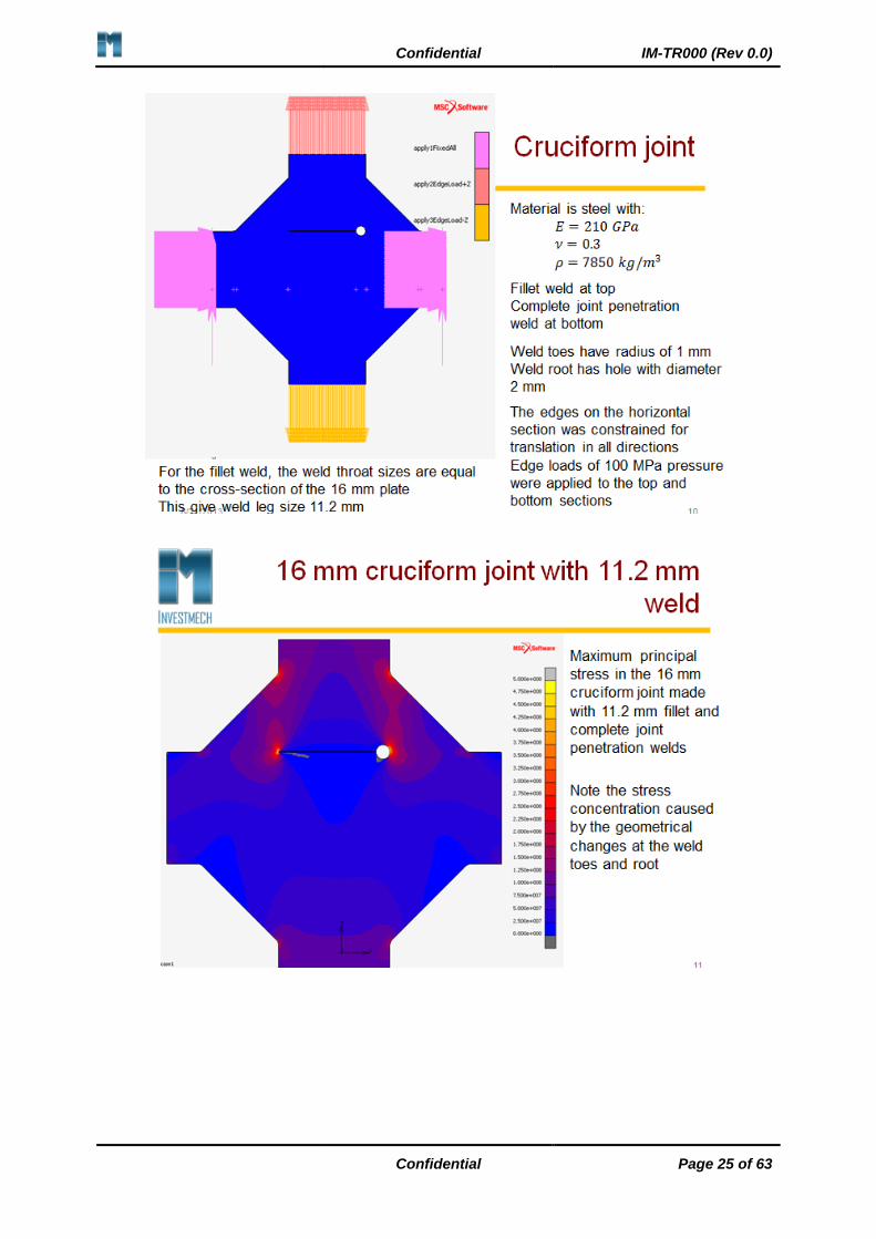
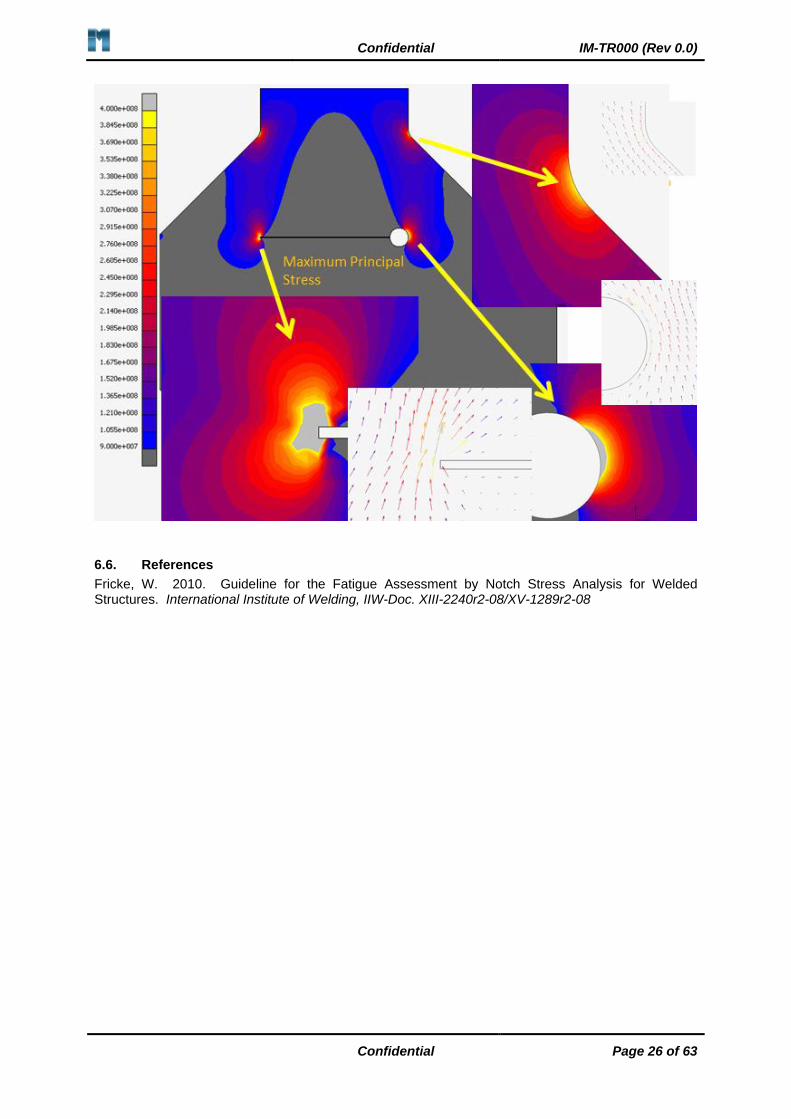
6.5. Applied to a cruciform joint
The slide below shows the finite element model with boundary conditions of a cruciform joint with:
1. The top weld left end sharp.
2. The top weld right end with notch radius 1.0 mm.
3. Complete joint penetration for the bottom weld.
Remember to always consider the direction of principal stresses in calculations.
Confidential IM-TR000 (Rev 0.0)
Confidential Page 25 of 63
Confidential IM-TR000 (Rev 0.0)
Confidential Page 26 of 63
6.6. References
Fricke, W. 2010. Guideline for the Fatigue Assessment by Notch Stress Analysis for Welded Structures. International Institute of Welding, IIW-Doc. XIII-2240r2-08/XV-1289r2-08
Confidential IM-TR000 (Rev 0.0)
Confidential Page 27 of 63
7. STATIC FAILURE THEORIES
The objective of this section is to provide revision of static failure theories used as acceptance criteria in design. Investmech assumes that these sections have been discussed in detail in applications by other lecturers and will not be repeated in detail.
This section covers the following:
• Calculation of principal stresses
• Static failure theories
• Buckling
• Variable loading
Always remember to include the design class of the structure in failure theories. For example, multiple load paths classify a structure as fail-safe, and other structures are designed for safe-life. In safe-life applications, damage tolerant design is essential.
Presentation used in
class:
Static Failure Criteria
Filename: Investmech - Structural Integrity (Static Failure Theories)
R0.0
7.1. Principal stress
Stress in any direction 𝑙, 𝑚 𝑎𝑛𝑑 𝑛 can be calculate for a multi-axial stress state using the following equation:
𝜎𝑛 = 𝑙2𝜎𝑥 + 𝑚2𝜎𝑦 + 𝑛2𝜎𝑧 + 2[𝑙𝑚𝜏𝑥𝑦 + 𝑛𝑙𝜏𝑥𝑧 + 𝑚𝑛𝜏𝑦𝑧] ( 14 )
Where, 𝑙, 𝑚 𝑎𝑛𝑑 𝑛 are the direction cosines of the unit vector directing in the direction in which the stress is required. The stress matrix is given as follows:
𝝈 = [
𝜎𝑥 −𝜎𝑥𝑦 −𝜎𝑥𝑧
−𝜎𝑦𝑥 𝜎𝑦 −𝜎𝑦𝑧
−𝜎𝑧𝑥 −𝜎𝑧𝑦 𝜎𝑧
] ( 15 )
There exists a direction where the shear stress components disappear and only normal stress remain. These directions and resulting normal stress are the principal axes and principal stresses respectively. The principal stresses are calculated from the eigenvalues of the stress matrix as follows:
|
𝜎 − 𝜎𝑥 −𝜎𝑥𝑦 −𝜎𝑥𝑧
−𝜎𝑦𝑥 𝜎 − 𝜎𝑦 −𝜎𝑦𝑧
−𝜎𝑧𝑥 −𝜎𝑧𝑦 𝜎 − 𝜎𝑧
| = 0
𝜎3 − 𝜎2(𝜎𝑥 + 𝜎𝑦 + 𝜎𝑧) + 𝜎(𝜎𝑥𝜎𝑦 + 𝜎𝑦𝜎𝑧 + 𝜎𝑥𝜎𝑧 − 𝜎𝑥𝑦2 − 𝜎𝑥𝑧
2 − 𝜎𝑦𝑧2 )
− (𝜎𝑥𝜎𝑦𝜎𝑧 + 2𝜎𝑥𝑦𝜎𝑥𝑧𝜎𝑦𝑧 − 𝜎𝑥𝜎𝑦𝑧2 − 𝜎𝑦𝜎𝑥𝑧
2 − 𝜎𝑧𝜎𝑥𝑦2 )
( 16 )
The eigenvalues, or principal stresses can be easily calculated in PC Matlab using the E=eig(X) command, where X is the stress matrix containing the numerical stress values in the sign convection shown in Equation 15.
For example, say the multi-axial stresses are as follows:
𝜎𝑥 = 600 𝑀𝑃𝑎 𝜎𝑦 = 0 𝑀𝑃𝑎
𝜎𝑧 = 0 𝑀𝑃𝑎 𝜎𝑥𝑦 = 400 𝑀𝑃𝑎
𝜎𝑥𝑧 = 0 𝑀𝑃𝑎 𝜎𝑦𝑧 = 0 𝑀𝑃𝑎
Then the matrix X is:
𝑋 = [600 − 400 0; −400 0 0; 0 0 0]
Performing this calculation in Matlab gives:
𝐸 = [−200 0 0
0 0 00 0 800
] ( 17 )
Confidential IM-TR000 (Rev 0.0)
Confidential Page 28 of 63
For a two dimensional problem, the maximum (𝜎1) and minimum (𝜎2) principal stresses can be calculated using the following equations:
𝜎1 =𝜎𝑥 + 𝜎𝑦
2+
1
2√(𝜎𝑥 − 𝜎𝑦)
2+ 4𝜏𝑥𝑦
2 ( 18 )
𝜎2 =𝜎𝑥 + 𝜎𝑦
2−
1
2√(𝜎𝑥 − 𝜎𝑦)
2+ 4𝜏𝑥𝑦
2 ( 19 )
The principal stresses are then ordered from large to small with 𝜎1, 𝜎2 𝑎𝑛𝑑 𝜎3 the maximum, intermediary and minimum principal stress.
7.2. Principal axes
The principal axes are easily determined by PC Matlab using the command: [V,D]=eig(x). The matrix D contains the eigenvalues and the columns of matrix V represent the eigenvectors in the coordinate system used to compile the stress matrix. For the previous values for X is used, this calculation gives:
>> [V,D]=eig(X)
V =
-0.4472 0 -0.8944
-0.8944 0 0.4472
0 1.0000 0
D =
-200 0 0
0 0 0
0 0 800
In this case the maximum principal stress is 𝜎1 = 800 𝑀𝑃𝑎 in the direction 𝑟1̅ = −0.8944𝑖̅ + 0.4472𝑗̅ +0�̅�. The minimum principal stress is 𝜎3 = −200 𝑀𝑃𝑎 in the direction 𝑟3̅ = −0.4472𝑖̅ − 0.8944𝑗̅ + 0�̅�.
In the following example the calculation is repeated for an obvious direction of the principal axes:
>> X=[600 0 0; 0 200 0; 0 0 100];
>> [V,D]=eig(X)
V =
0 0 1
0 1 0
1 0 0
D =
100 0 0
0 200 0
0 0 600
In this case the maximum principal stress is 𝜎1 = 600 𝑀𝑃𝑎 and the minimum stress is 𝜎3 = 100 𝑀𝑃𝑎.
The direction of the principal axles is clear in this case. For example, 𝑟1̅ = 1𝑖̅ + 0𝑗̅ + 0�̅� for the stress 𝜎1 = 600 𝑀𝑃𝑎. That is the, the third column of V aligns with the third column (and row) where D = 600 MPa.
These mathematics are carried out on the multi-axial stress state at a point to find the principal stresses and their associated directions relative to the coordinate system used to construct the stress matrix.
7.3. Failure theories
7.3.1. Maximum normal stress
In this case the maximum principal stresses are compared against the material resistances. The maximum and minimum principal stress is 𝜎1 and 𝜎3 respectively, where 𝜎1 and 𝜎3 are not necessarily in tension or compression. Consider the unique situation of hydrostatic stress where 𝜎1 = 𝜎2 = 𝜎3. Acceptance criteria are normally the material’s yield or ultimate strength or a factor thereof. For example, the partial factor for strength in SANS 10162-1 is 𝜙 = 0.9 for structural steel sections.
Confidential IM-TR000 (Rev 0.0)
Confidential Page 29 of 63
Where both tensile and compressive stresses are present, tensile and compressive material resistance must be used.
7.3.2. Maximum shear stress
The maximum shear stress is:
𝜏𝑚𝑎𝑥 =𝜎1 − 𝜎3
2 ( 20 )
Failure occurs when the maximum shear stress exceeds the fracture stress, 𝜎𝑓:
𝜏𝑚𝑎𝑥 ≥𝜎𝑓
2
𝑜𝑟 |𝜎1 − 𝜎2| ≥ 𝜎𝑓 |𝜎1 − 𝜎3| ≥ 𝜎𝑓 |𝜎3 − 𝜎2| ≥ 𝜎𝑓
( 21 )
Normally the yield strength, ultimate strength or factors thereof are used for the fracture strength.
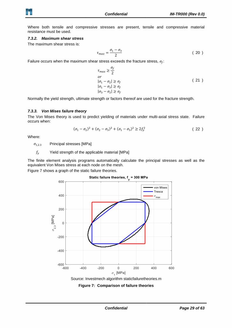
7.3.3. Von Mises failure theory
The Von Mises theory is used to predict yielding of materials under multi-axial stress state. Failure occurs when:
(𝜎1 − 𝜎2)2 + (𝜎2 − 𝜎3)2 + (𝜎1 − 𝜎3)2 ≥ 2𝑓𝑦2 ( 22 )
Where:
𝜎1,2.3 Principal stresses [MPa]
𝑓𝑦 Yield strength of the applicable material [MPa]
The finite element analysis programs automatically calculate the principal stresses as well as the equivalent Von Mises stress at each node on the mesh.
Figure 7 shows a graph of the static failure theories.
Source: Investmech algorithm staticfailuretheories.m
Figure 7: Comparison of failure theories

Confidential IM-TR000 (Rev 0.0)
Confidential Page 30 of 63
7.3.4. Octahedral shear stress theory
The octahedral shear stress predicts failure exactly as the von Mises failure theory given above.
𝜏𝑜𝑐𝑡 =1
3√(𝜎1 − 𝜎2)2 + (𝜎2 − 𝜎3)2 + (𝜎1 − 𝜎3)2 ≥
√2
3𝑓𝑦 ( 23 )
7.3.5. Mohr’s failure theory
The Mohr’s failure theory is also known as the Coulomb-Mohr criterion or the internal friction theory, and, is based on the Mohr circle shown below. The angle of radius 𝑅 with the horizontal is 2𝜃 and is used to find the plane of maximum stress. This indicates that if only shear stress is applied, the maximum principal stress will be on an angle of 45° because 2𝜃 = 90°.
Case Principal stresses Acceptance criterion
1 Both in tension 𝜎1 > 0,
𝜎2 > 0
𝜎1 < 𝜎𝑡 , 𝜎2 < 𝜎𝑡
2 Both in compression 𝜎1 < 0,
𝜎2 < 0
𝜎1 > −𝜎𝑐, 𝜎2 > −𝜎𝑐
3 𝜎1 in tension, 𝜎2 in compression 𝜎1 > 0,
𝜎2 < 0
𝜎1
𝜎𝑡
+𝜎2
−𝜎𝑐
< 1
4 𝜎1 in compression, 𝜎2 in tension 𝜎1 < 0,
𝜎2 > 0
𝜎1
−𝜎𝑐
+𝜎2
𝜎𝑡
< 1
Mohr’s versus the maximum stress criterion will be explained in class according to the sketch below.
7.3.6. These are not all
Note that there are several other static failure theories applied by Investmech that are not presented here. For example, additional failure theories include:
• Maximum normal strain theory (St. Venant’s theory)
• Total strain energy theory (Beltrami theory)
• Etc.
7.3.7. Which static theory can be used
Research showed that for:
1. Ductile material types (> 5 % elongation at break):
a. The maximum shear stress criterion and the von Mises criterion are accurate static failure theories

Confidential IM-TR000 (Rev 0.0)
Confidential Page 31 of 63
2. Brittle material types (≤ 5 % elongation at break):
a. The maximum normal stress criterion and the Mohr’s theory provide accurate results.
Investmech always applies the maximum principal stress theory and the von Mises theory for static design. The use of the von Mises theory without the maximum normal stress theory could result in wrong answers because of the way in which the von Mises equation eliminates hydrostatic stress conditions.
For crashworthiness, furnace design, or other applications where there is substantial plastic deformation, the maximum engineering strain and true principal strains are used.
7.4. Buckling
Columns under compressive loading have a length dependent critical load where the section will fail under buckling. A vertical column hinged at the bottom has a critical load of:
𝑃𝑐𝑟 =𝜋2𝐸𝐼
𝐿2 ( 24 )
Different equations exist for the different boundary conditions and should be applied according to the constraints relevant to the practical problem.
7.5. Non stress-based criteria
There is several other mission profile driven criteria that also need to be considered in the design of structures. For example:
• Success of parts not necessarily determined by strength
o Stiffness, vibrational characteristics, fatigue resistance, creep resistance
• Examples
o Rigidity in automotive vehicles
o Weight reduction in bicycles
o Patio deck – stiffness to prevent excessive deformation
7.6. Conclusion
• Always look at all failure criteria, or at least two:
o The one that prevails first will be the mode in which failure will occur
• For furnaces, the maximum total strain of 20% is used to quantify the number of heat-up cycles
• Fatigue analysis is concerned with the calculation of damage to the structure and is the life until a detectable crack initiates.
• Fracture Mechanics determines failure during the crack growth phase.
8. VARIABLE AMPLITUDE LOADING
The objective of this section is to provide an understanding of the analysis of dynamic loads on structures.
The scope of the work includes:
1. Types of loading.
2. Statistical stress analysis on real structures.
3. Stress collective, S-N curve.
4. Mean stress calculation and its effect
After completion of this section you will be able to:
1. Describe methods of counting load cycles.
2. Calculate stress ration and other statistical parameters.
Presentation used in class:
Variable Amplitude Loading
Filename: Investmech - Structural Integrity (Variable Amplitude Loading) R0.0

Confidential IM-TR000 (Rev 0.0)
Confidential Page 32 of 63
8.1. Types of loading
Loads can be tensile loads, compressive loads and/or shear loads (torsion) that produce stress and deformation of the component.
Loads can be divided into the following:
• Static load
– Do not change over time
– SANS 10160-1 and other standard refer to static loads as dead- or permanent loads or actions.
• Quasi-static load
– Applied at rate lower than lowest natural period of the structure
– Investmech uses a load application period of 5 times the lowest natural period as a quasi-static load. The is equal to a frequency of 1/5th the lowest natural frequency.
• Dynamic loads
– Load application period shorter than 5 × lowest natural period, and typically cause force effects due to natural modes
– Shock load
• Impact load period significantly shorter than the natural period
8.2. Causes for loads on structures
There are many causes for variable amplitude loads on structures of which the following is a typical list:
• Thermal
– Normally quasi-static
– Can be deterministic
• Process activities
– Random, but steady-state
• Wind loads
• Cavitation
• Fluid-structural interactions
– Water-hammer
– Tidal – normally quasi-static of nature
– Waves
• Mechanical loads
– unbalance, misalignment, screen suspension, crusher supports, impact hammers, etc.
• Human interactions
– Dropping objects, explosions, crushes, etc.
• Cluster events (Storms, process in reactors, accidents, derailing of railway vehicles, etc.)
• Etc.
8.3. Loads and stress-strain
Loads are converted to stress. The stress can be determined in typically the following ways:
• Elementary equations:
– Normal stress: 𝜎𝑛 =𝐹
𝐴
– Bending stress: 𝜎𝑏 =𝑀𝑥𝑦
𝐼𝑥𝑥−
𝑀𝑦𝑥
𝐼𝑦𝑦
– Shear stress (Torsion): 𝜏 =𝑉𝑄
𝐴+
𝑇𝑟
𝐽, note the directions!
• Finite element analysis
• Strain measurement and conversion to stress
Confidential IM-TR000 (Rev 0.0)
Confidential Page 33 of 63
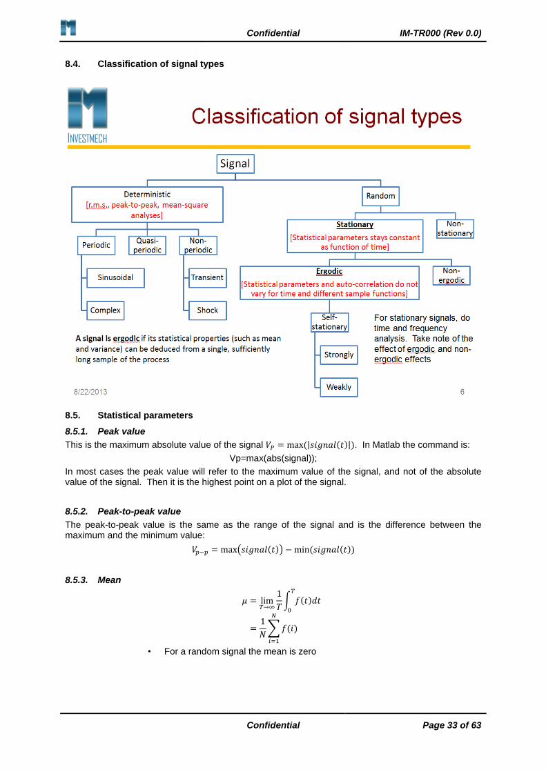
8.4. Classification of signal types
8.5. Statistical parameters
8.5.1. Peak value
This is the maximum absolute value of the signal 𝑉𝑃 = max (|𝑠𝑖𝑔𝑛𝑎𝑙(𝑡)|). In Matlab the command is:
Vp=max(abs(signal));
In most cases the peak value will refer to the maximum value of the signal, and not of the absolute value of the signal. Then it is the highest point on a plot of the signal.
8.5.2. Peak-to-peak value
The peak-to-peak value is the same as the range of the signal and is the difference between the maximum and the minimum value:
𝑉𝑝−𝑝 = max(𝑠𝑖𝑔𝑛𝑎𝑙(𝑡)) − min (𝑠𝑖𝑔𝑛𝑎𝑙(𝑡))
8.5.3. Mean
𝜇 = lim𝑇→∞
1
𝑇∫ 𝑓(𝑡)𝑑𝑡
𝑇
0
=1
𝑁∑ 𝑓(𝑖)
𝑁
𝑖=1
• For a random signal the mean is zero

Confidential IM-TR000 (Rev 0.0)
Confidential Page 34 of 63
8.5.1. Root-mean-square
𝑅𝑀𝑆 = √ lim𝑇→∞
1
𝑇∫ 𝑓(𝑡)2𝑑𝑡
𝑇
0
= √1
𝑁∑ 𝑓(𝑖)2
𝑁
𝑖=1
• Gives the intensity of the data which is an indication of the energy
• This is an Overall Value, that is, one value that describes the characteristic of all the values
• With band-pass filter will give narrow-band intensity
8.5.2. Crest factor
𝐶𝐹 =𝑃𝑒𝑎𝑘 𝑜𝑓 𝑡ℎ𝑒 𝑠𝑖𝑔𝑛𝑎𝑙
𝑅𝑀𝑆
• For a pure sine wave cf = 2(1/2)
• A cf > 3 indicates on irregularities in the signal
• The cf is not monotome
o Will not necessarily increase with an increase in RMS
• Used to describe the “peakiness” of a function/signal
8.5.3. Variance and standard deviation
𝜎2 = lim𝑇→∞
1
𝑇∫(𝑓(𝑡) − 𝜇)2𝑑𝑡
𝑇
0
=1
𝑁∑(𝑓(𝑖) − 𝜇)2
𝑁
𝑖=1
Variance = (standard deviation)2 = σ2
The standard deviation quantifies the distribution of data points around the mean.
8.5.4. Kurtosis
𝐾𝑈 =1
𝜎4lim𝑇→∞
1
𝑇∫(𝑓(𝑡) − 𝜇)4𝑑𝑡
𝑇
0
=1
𝜎4×
1
𝑁∑(𝑓(𝑖) − 𝜇)4
𝑁
𝑖=1
• The kurtosis is not monotome
• Describe the peakiness of a signal
• For sine wave KU=2
• For a random signal KU=1.5
8.5.5. Example
Space allowed for class problem on time domain analysis
Sample record given: -1; -0,5; 0; 0,5; 1; 0,75; 0,5; 0,2; -0,2
Peak-to-peak value

Confidential IM-TR000 (Rev 0.0)
Confidential Page 35 of 63
Mean
RMS
Standard deviation
Crest factor
8.6. Presentation of stress data
It is important that stress data is accurate. Stress data for fatigue calculation is normally presented as the stress ranges with the number of occurrences in the signal. That is, a table with the one column containing stress ranges and the next column the number of times that the specific stress range occurred in the signal. Stress data can also be presented as a spectrum using FFT calculations. This is only accurate for steady-state responses. In most cases the actual stress signal is not known exactly, but, can be accurately described by the mean and standard deviation.
8.7. Stress histories
The sketch below provides a list of typical stress histories.

Confidential IM-TR000 (Rev 0.0)
Confidential Page 36 of 63
8.8. Obtaining stress spectra for fatigue calculations
With computing power today, measured strains converted to stress can be used directly to calculate the stress spectrum for the measurement point.
Load spectra for stress measured or from transient analysis:
• PSD or Spectral analysis
– Note, the results is for a specific period and must be scaled!
• Counting methods
• Peak counting, Mean-crossing peak count, Range pair count, Range-pair-mean count, Rainflow count, Reservoir counting method
– The counting method must produce the correct crack initiation and growth result
– Counting method must detect peak, mean, minimum, and maximum of signal
– The results are presented in a histogram for Δ𝜎𝑅 and 𝑛𝑅
– Note, the results is also only for the duration of the signal measured and must be scaled
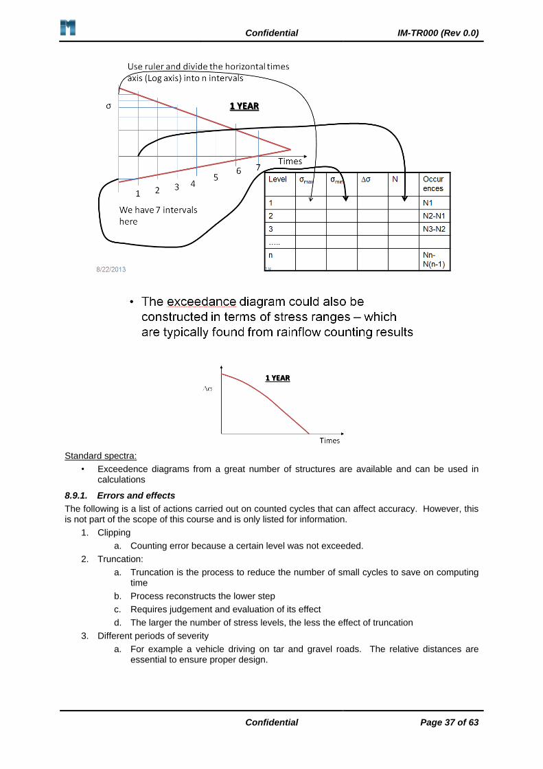
8.9. Exceedence diagrams
This is beyond the scope of this course and is only presented in class as an example.
Confidential IM-TR000 (Rev 0.0)
Confidential Page 37 of 63
Standard spectra:
• Exceedence diagrams from a great number of structures are available and can be used in calculations
8.9.1. Errors and effects
The following is a list of actions carried out on counted cycles that can affect accuracy. However, this is not part of the scope of this course and is only listed for information.
1. Clipping
a. Counting error because a certain level was not exceeded.
2. Truncation:
a. Truncation is the process to reduce the number of small cycles to save on computing time
b. Process reconstructs the lower step
c. Requires judgement and evaluation of its effect
d. The larger the number of stress levels, the less the effect of truncation
3. Different periods of severity
a. For example a vehicle driving on tar and gravel roads. The relative distances are essential to ensure proper design.

Confidential IM-TR000 (Rev 0.0)
Confidential Page 38 of 63
8.10. Variable amplitude loading
• Most service loading histories have variable amplitude
• Sometimes stochastic of nature (random probability distribution, may be analysed statistically but cannot be predicted precisely)
• The following aspects need to be addressed:
– Nature of fatigue damage and how it can be related to load history
– Damage summation methods
– Cycle counting techniques to recognise damaging events
– Crack propagation behaviour under variable amplitude loading
– How to deal with service load histories
• Fatigue is the tendency of materials to fail due to cracks that initiates and propagates
• Definition of fatigue damage
– The measurable propagation portion of fatigue
• Damage is directly related to crack length it is observable, measurable
• Inspection intervals used to monitor crack growth
– Initiation phase
• Mechanisms on microscopic level (dislocations, slip bands, micro-cracks, etc.)
• Only measurable in highly controlled laboratory environment
Most damage summing methods during initiation phase empirical of nature
8.11. Cycle counting methods – discussed
The objective of cycle counting techniques for fatigue analysis is to reduce the data required in analysis. For example, in a strain/stress signal for fatigue analysis, the turning points (extrema) are required, not the data points in between.
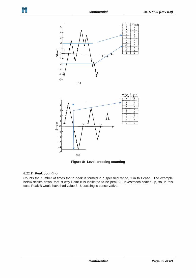
8.11.1. Level crossing
Number of times that strain or stress of certain value is crossed. Can be done on the original signal or range levels.
Confidential IM-TR000 (Rev 0.0)
Confidential Page 39 of 63
Figure 8: Level-crossing counting
8.11.2. Peak counting
Counts the number of times that a peak is formed in a specified range, 1 in this case. The example below scales down, that is why Point B is indicated to be peak 2. Investmech scales up, so, in this case Peak B would have had value 3. Upscaling is conservative.

Confidential IM-TR000 (Rev 0.0)
Confidential Page 40 of 63
Figure 9: Peak-counting
8.11.3. Simple-range counting
Figure 10: Simple-range counting
Confidential IM-TR000 (Rev 0.0)
Confidential Page 41 of 63
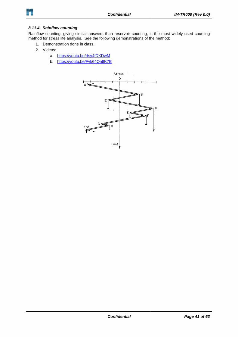
8.11.4. Rainflow counting
Rainflow counting, giving similar answers than reservoir counting, is the most widely used counting method for stress life analysis. See the following demonstrations of the method:
1. Demonstration done in class.
2. Videos:
a. https://youtu.be/rIsy4fDXDwM
b. https://youtu.be/Fvk64Qn9K7E

Confidential IM-TR000 (Rev 0.0)
Confidential Page 42 of 63
8.11.5. Sequence effects
Strain-time histories may yield very different stress-strain responses, especially in notches where plasticity occurs as shown in Figure 11. Level-crossing, peak-counting and simple range counting do not include sequence effects. If the rainflow counting algorithm is applied in sequence, it does include sequence effects (from-to values in the Markov matrix from which mean, amplitude and range can be calculated), one of the reasons why it is used widely. For these situations, the strain dependent residual strains in the notch need to be modelled, for which strain life principles are used.
Figure 11: Load sequence effects
8.11.6. More info on Rainflow counting
– A number of rainflow counting techniques are in use
– If the strain-time history being analyzed begins and ends at the strain value having the largest magnitude, whether it occurs at a peak or a valley, all of the rainflow counting techniques yield identical results
– Develop the Markov Matrix and find strain amplitudes and mean stress
– Use the Morrow equation to solve the fatigue life at each strain level:
Δ𝜖
2=
𝜎𝑓′ − 𝜎𝑜
𝐸[2𝑁𝑓]
𝑏+ 𝜖𝑓
′ [2𝑁𝑓]𝑐
– Calculate cumulative damage from Miner’s rule: 𝐷 = ∑0.5
𝑁𝑓≥ 1, note, reversals = half cycles are
used in the Morrow equation
– ASTM standard for Rainflow counting in literature
Confidential IM-TR000 (Rev 0.0)
Confidential Page 43 of 63
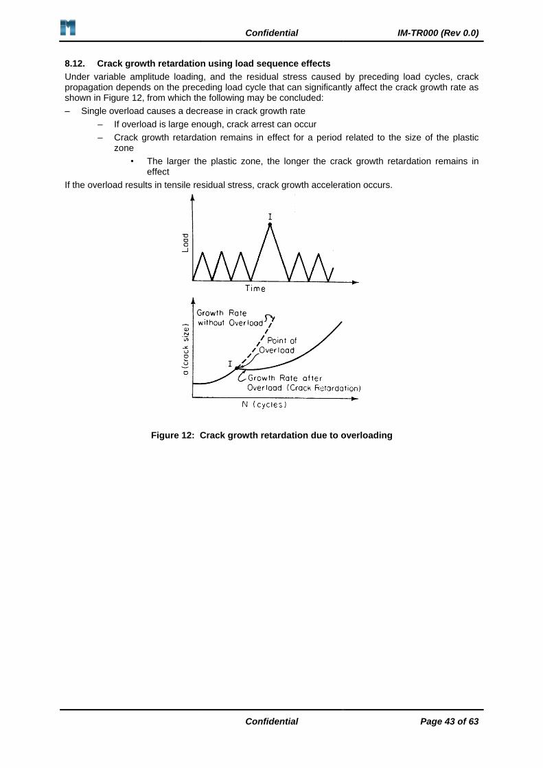
8.12. Crack growth retardation using load sequence effects
Under variable amplitude loading, and the residual stress caused by preceding load cycles, crack propagation depends on the preceding load cycle that can significantly affect the crack growth rate as shown in Figure 12, from which the following may be concluded:
– Single overload causes a decrease in crack growth rate
– If overload is large enough, crack arrest can occur
– Crack growth retardation remains in effect for a period related to the size of the plastic zone
• The larger the plastic zone, the longer the crack growth retardation remains in effect
If the overload results in tensile residual stress, crack growth acceleration occurs.
Figure 12: Crack growth retardation due to overloading
Confidential IM-TR000 (Rev 0.0)
Confidential Page 44 of 63
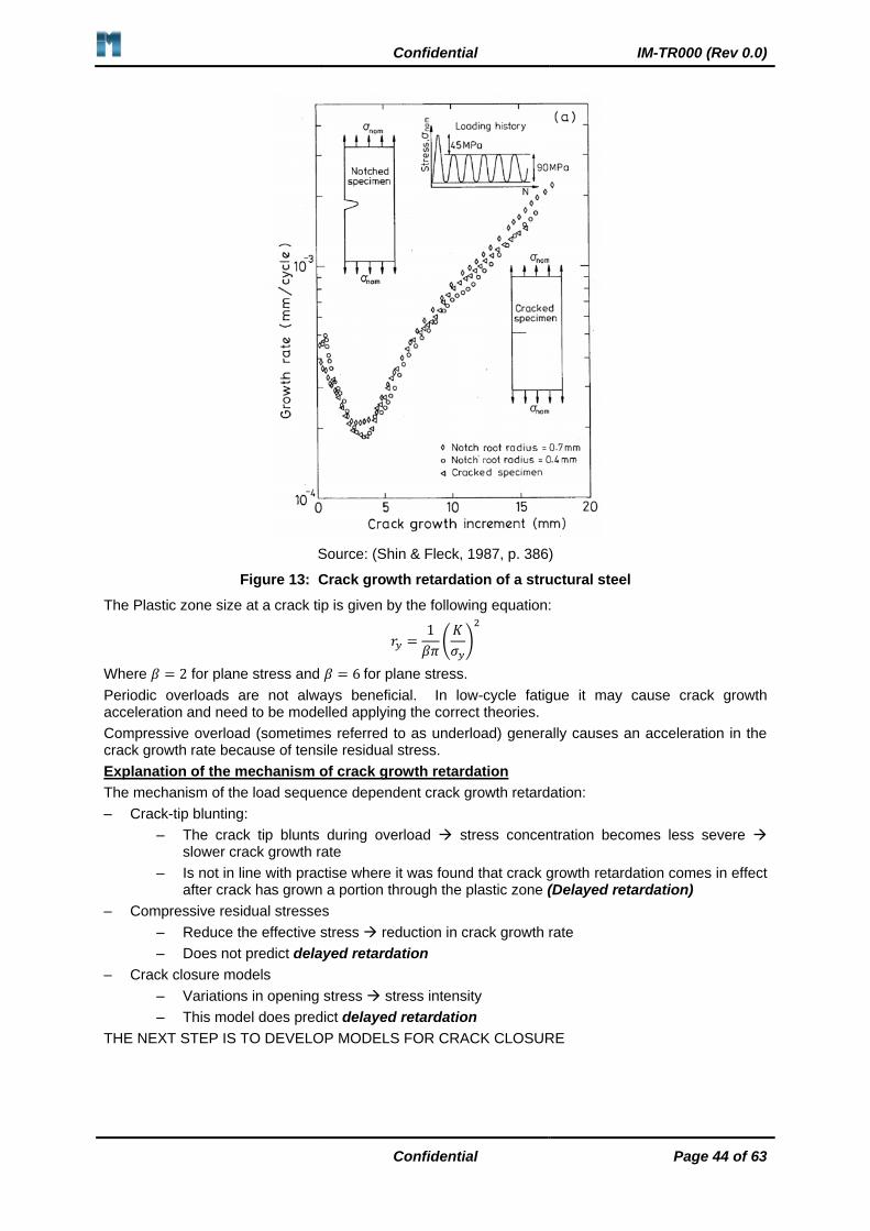
Source: (Shin & Fleck, 1987, p. 386)
Figure 13: Crack growth retardation of a structural steel
The Plastic zone size at a crack tip is given by the following equation:
𝑟𝑦 =1
𝛽𝜋(
𝐾
𝜎𝑦)
2
Where 𝛽 = 2 for plane stress and 𝛽 = 6 for plane stress.
Periodic overloads are not always beneficial. In low-cycle fatigue it may cause crack growth acceleration and need to be modelled applying the correct theories.
Compressive overload (sometimes referred to as underload) generally causes an acceleration in the crack growth rate because of tensile residual stress.
Explanation of the mechanism of crack growth retardation
The mechanism of the load sequence dependent crack growth retardation:
– Crack-tip blunting:
– The crack tip blunts during overload stress concentration becomes less severe slower crack growth rate
– Is not in line with practise where it was found that crack growth retardation comes in effect after crack has grown a portion through the plastic zone (Delayed retardation)
– Compressive residual stresses
– Reduce the effective stress reduction in crack growth rate
– Does not predict delayed retardation
– Crack closure models
– Variations in opening stress stress intensity
– This model does predict delayed retardation
THE NEXT STEP IS TO DEVELOP MODELS FOR CRACK CLOSURE

Confidential IM-TR000 (Rev 0.0)
Confidential Page 45 of 63
8.12.1. Crack growth retardation prediction methods
In tests done on structural steels, it was found that when the baseline stress intensity range, Δ𝐾, is
much greater than the threshold stress intensity, Δ𝐾𝑡ℎ and plane stress conditions prevail, growth retardation is primarily due to plasticity-induced crack closure (Shin & Fleck, 1987, p. 392). For lower baseline stress intensity, Δ𝐾𝑏 close to the threshold stress intensity and plane strain conditions apply, an overload produces immediate crack arrest at the surface of the specimen, cut, not in the bulk of the specimen. Shin & Fleck postulated that this is due to combination of strain hardening and residual stress at the crack tip.
Figure 14: Crack-tip plasticity
The following approaches are typically used:
– Statistical Methods
– Use the root mean square stress intensity factor
– Only applicable to short spectra
– Do not account for load sequence effects
– Very restricted application
– Does not predict crack growth retardation
– Crack closure models
– Does predict crack growth retardation
– Must estimate the opening stress for variable loading
– Must be done cycle for cycle
– Good correlation has been obtained
8.12.2. Further reading
(Carlson, Kardomateas, & Bates, 1991)
(Shin & Fleck, 1987)
8.13. Block loading
The application of block loading will be explained in class problems on fatigue. The principle behind block loading is to calculated damager per day, month, year, take-off-flight-landing, etc. event, and then calculated the number of times that the modelled event can be repeated. For the automotive industry one block is typically a mission profile driven length of route with known test route severity rating.
Block loading:
– Use blocks instead of cycle-for-cycle counting
– Considerable savings in time
– Limited to short spectra of loading
– Crack growth per block less than the plastic zone caused by the largest load cycle
– Damage is assumed to occur only when the crack is open
– The crack opening stress must be determined
Confidential IM-TR000 (Rev 0.0)
Confidential Page 46 of 63
– This means use of the change in positive stress intensity
• Compressive residual stress beneficial
Dealing with service histories:
• Sometimes the service load history is unknown
• A representative load history or loading block may be determined from field tests
– Analytical construction of service loads also done
• Fatigue life, or damage may then be calculated from the load blocks
Method: SAE Cumulative Damage Test program
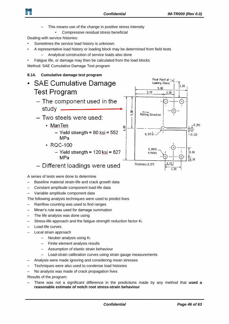
8.14. Cumulative damage test program
A series of tests were done to determine
– Baseline material strain-life and crack growth data
– Constant amplitude component load-life data
– Variable amplitude component data
The following analysis techniques were used to predict lives
– Rainflow counting was used to find ranges
– Miner’s rule was used for damage summation
– The life analysis was done using
– Stress-life approach and the fatigue strength reduction factor Kf
– Load-life curves
– Local strain approach
– Neuber analysis using Kf
– Finite element analysis results
– Assumption of elastic strain behaviour
– Load-strain calibration curves using strain gauge measurements
– Analysis were made ignoring and considering mean stresses
– Techniques were also used to condense load histories
– No analysis was made of crack propagation lives
Results of the program:
– There was not a significant difference in the predictions made by any method that used a reasonable estimate of notch root stress-strain behaviour

Confidential IM-TR000 (Rev 0.0)
Confidential Page 47 of 63
– Good predictions were made using the Neuber approach that tended to be slightly conservative
– There was not a large difference between predictions which included and excluded mean stresses
– Predictions made using the simple stress-life approach showed correlation which was as good as those predicted by more complicated techniques
– Another study showed that the following method predicted very good propagation lives
– Use FEA to determine crack opening levels
– Rainflow counting + Linear Elastic Fracture Mechanics (LEFM)
8.15. Conclusion
• Miner’s linear damage rule provides reasonable life estimates
• Most effective cycle counting procedures relate damaging events to the stress-strain response of the material (Like Rainflow counting)
• Repeated block loading analysis techniques may be applied to save time
• Application of large overloads may cause crack growth retardation
9. CYCLE COUNTING WITH THE RAINFLOW METHOD
During this section Investmech will demonstrate to the student how the rainflow counting method works and how Matlab is applied in rainflow counting. For the purpose of this course the student is not expected to perform cycle counting, however, the student must be able to demonstrate the rainflow counting method.
Note, it is expected from the student to make notes of the rainflow counting method as explained by the lecturer in class. Notes will not be issued in class.
Presentation used in class: Cycle counting at Investmech
Filename: Investmech - Structural Integrity (Cycle counting) R0.0
Use the remainder of this page and the following page to make notes during the lecture.

Confidential IM-TR000 (Rev 0.0)
Confidential Page 48 of 63
Leave open for notes.

Confidential IM-TR000 (Rev 0.0)
Confidential Page 49 of 63
10. STRESS LIFE ANALYSIS
This section introduces stress life analysis.
Presentation used in class: Investmech - Fatigue (Stress life analysis) R0.0
Discuss according to slides. The remainder of this section summarises problems done in class.
10.1. Slides not in notes
There are several slides presented in class that are not in the notes. Please download the slides to obtain digital copies of these slides. They are informative of nature, but, important and include:
– Total life curve
– Images of fracture surfaces
Notes from the lecture:

Confidential IM-TR000 (Rev 0.0)
Confidential Page 50 of 63
10.2. Notches
In general you were introduced to static failure criteria, of which maximum principal stress, von Mises and Tresca (maximum shear stress theory) are the most widely used theories. The stress-life approach cannot account for load sequence events, which can be modelled by the strain-life method. Local stress concentrations and residual stress are also accounted for in the strain-life method. Fracture mechanics is applied to modelled crack propagation after crack initiation.
10.2.1. Weld toes
Stress concentrations exist at weld toes. Accurate modelling of these stress concentration under low loads allows the use of the general fatigue curve. It is clear that cracks will initiate at the highest stressed points, which are mostly in the stress concentrations. Weld toes leave geometry that produce stress concentrations, the reason why cracks initiate in weld toes.
Source: (Taylor, Barrett, & Lucano, 2002)
Figure 15: Stress concentrations at weld toes result in crack initiation
10.3. Theoretic stress concentration factor
Stress concentrations (with theoretical stress concentration, 𝐾𝑡) due to geometrical or micro-structural discontinuities result in higher local stress, 𝜎𝑠𝑐, than the nominal stress away from the stress
concentration, 𝜎:
𝜎𝑚𝑎𝑥 = 𝐾𝑡𝜎
𝐾𝑡 =𝜎𝑠𝑐
𝜎
( 25 )
The ration between the maximum local stress and the nominal stress in a notched material is the theoretical stress concentration factor, 𝐾𝑡. 𝐾𝑡 is dependent on the geometry and the model of loading. Theoretical stress concentration factors for various geometries and modes of loading can be seen in Figure 16.
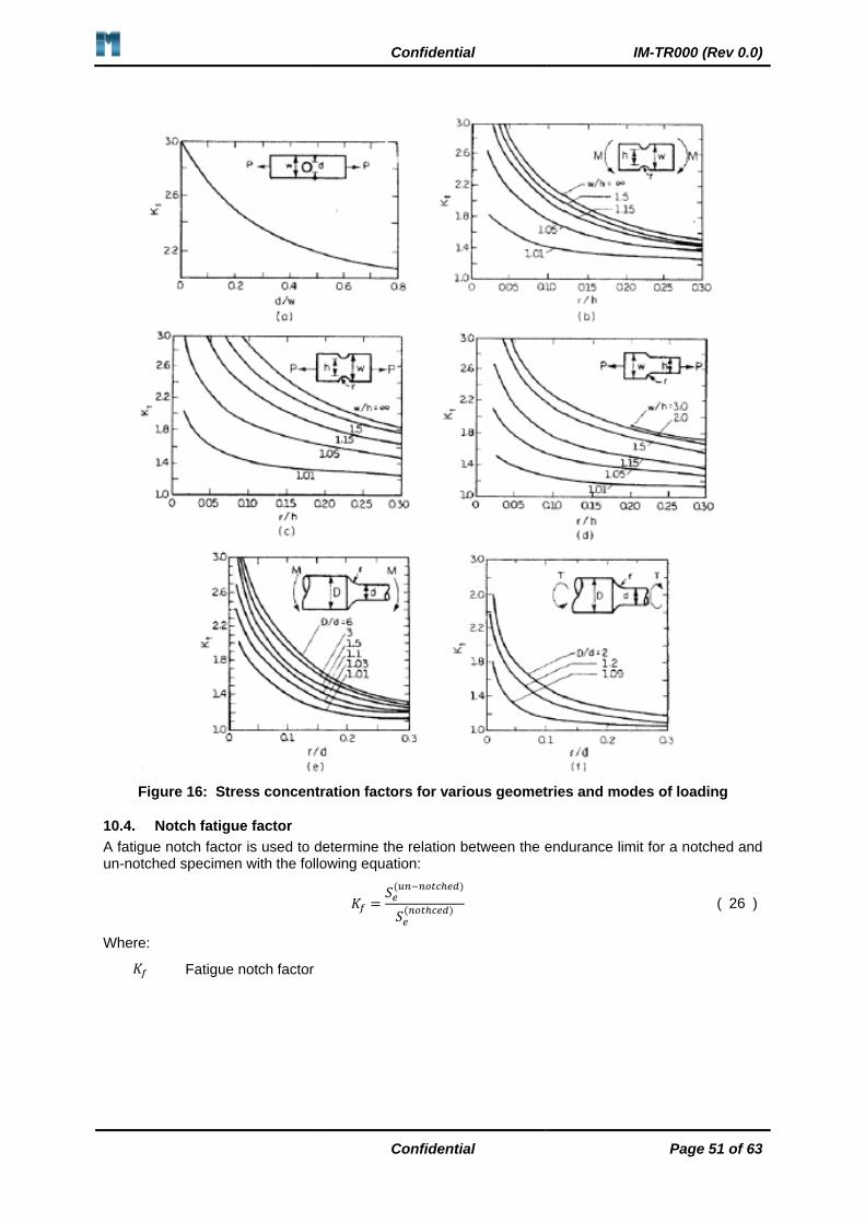
Confidential IM-TR000 (Rev 0.0)
Confidential Page 51 of 63
Figure 16: Stress concentration factors for various geometries and modes of loading
10.4. Notch fatigue factor
A fatigue notch factor is used to determine the relation between the endurance limit for a notched and un-notched specimen with the following equation:
𝐾𝑓 =𝑆𝑒
(𝑢𝑛−𝑛𝑜𝑡𝑐ℎ𝑒𝑑)
𝑆𝑒(𝑛𝑜𝑡ℎ𝑐𝑒𝑑)
( 26 )
Where:
𝐾𝑓 Fatigue notch factor

Confidential IM-TR000 (Rev 0.0)
Confidential Page 52 of 63
The fatigue notch factor is also dependent on material type and can be calculated using the following equation:
𝐾𝑓 = 1 +𝐾𝑡 − 1
(1 +𝑎
𝑟)
𝑎 = [300
𝑓𝑢[𝑘𝑠𝑖]]
1.8
×10−3 𝑖𝑛.
( 27 )
Where:
𝑎 Factor depending on the material used [mm]
𝑟 Notch radius [mm]
The fatigue notch factor can be used to adjust the S-N curve as can be seen in Figure 17.
Figure 17: S-N curve adjusted for a notched material
Ultimately, stress concentrations occurring from geometric discontinuities significantly lower than the fatigue life and endurance limit of a material.
An example of a finite element analysis done on a plate with a hole in the middle can be seen in Figure 18.
The applicable dimensions for the plate are:
• Hole diameter (𝑑): 20 mm.
• Plate width (𝑤): 50 mm.
This example demonstrates the stress concentration that exists in the regions next to the hole. The plate was loaded with a nominal stress of 100 MPa, and from Figure 18 it can be seen that the
maximum stress is 334 MPa. The nominal stress in that area of the hole is 100×50
30= 167 𝑀𝑃𝑎 and
thus, the stress concentration factor is 334
167= 2 according to the finite element analysis.
The same problem can be assessed with the stress concentration factors as can be seen in Figure 16.
Thus the ratio is equal to 𝑑
𝑤=
20
50= 0.4 and from Figure 19 it can be seen that the stress concentration
𝑆103
𝑆103/𝐾𝑓′
𝑆𝑒/𝐾𝑓
𝑆𝑒
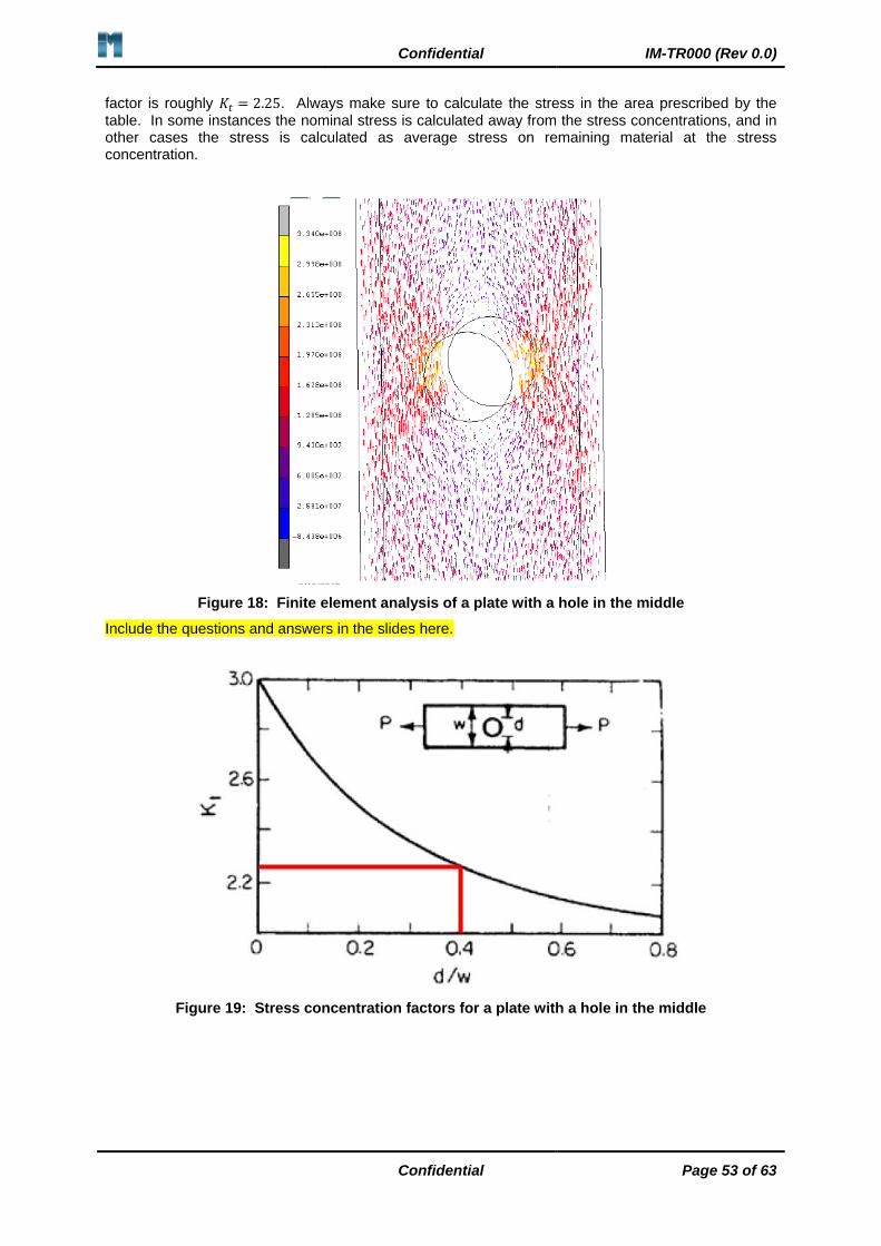
Confidential IM-TR000 (Rev 0.0)
Confidential Page 53 of 63
factor is roughly 𝐾𝑡 = 2.25. Always make sure to calculate the stress in the area prescribed by the table. In some instances the nominal stress is calculated away from the stress concentrations, and in other cases the stress is calculated as average stress on remaining material at the stress concentration.
Figure 18: Finite element analysis of a plate with a hole in the middle
Include the questions and answers in the slides here.
Figure 19: Stress concentration factors for a plate with a hole in the middle
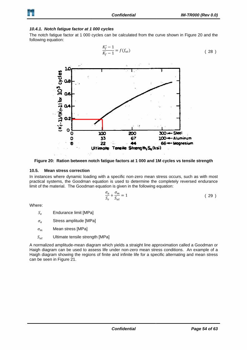
Confidential IM-TR000 (Rev 0.0)
Confidential Page 54 of 63
10.4.1. Notch fatigue factor at 1 000 cycles
The notch fatigue factor at 1 000 cycles can be calculated from the curve shown in Figure 20 and the following equation:
𝐾𝑓′ − 1
𝐾𝑓 − 1= 𝑓(𝑓𝑢𝑡) ( 28 )
Figure 20: Ration between notch fatigue factors at 1 000 and 1M cycles vs tensile strength
10.5. Mean stress correction
In instances where dynamic loading with a specific non-zero mean stress occurs, such as with most practical systems, the Goodman equation is used to determine the completely reversed endurance limit of the material. The Goodman equation is given in the following equation:
𝜎𝑎
𝑆𝑒+
𝜎𝑚
𝑆𝑢𝑡= 1 ( 29 )
Where:
𝑆𝑒 Endurance limit [MPa]
𝜎𝑎 Stress amplitude [MPa]
𝜎𝑚 Mean stress [MPa]
𝑆𝑢𝑡 Ultimate tensile strength [MPa]
A normalized amplitude-mean diagram which yields a straight line approximation called a Goodman or Haigh diagram can be used to assess life under non-zero mean stress conditions. An example of a Haigh diagram showing the regions of finite and infinite life for a specific alternating and mean stress can be seen in Figure 21.
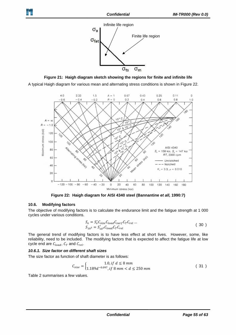
Confidential IM-TR000 (Rev 0.0)
Confidential Page 55 of 63
Figure 21: Haigh diagram sketch showing the regions for finite and infinite life
A typical Haigh diagram for various mean and alternating stress conditions is shown in Figure 22.
Figure 22: Haigh diagram for AISI 4340 steel (Bannantine et all, 1990:7)
10.6. Modifying factors
The objective of modifying factors is to calculate the endurance limit and the fatigue strength at 1 000 cycles under various conditions.
𝑆𝑒 = 𝑆𝑒′ 𝐶𝑠𝑖𝑧𝑒𝐶𝑙𝑜𝑎𝑑𝐶𝑠𝑢𝑟𝑓𝐶𝑇𝐶𝑟𝑒𝑙 …
𝑆103 = 𝑆103′ 𝐶𝑙𝑜𝑎𝑑𝐶𝑇𝐶𝑟𝑒𝑙
( 30 )
The general trend of modifying factors is to have less effect at short lives. However, some, like reliability, need to be included. The modifying factors that is expected to affect the fatigue life at low cycle end are 𝐶𝑙𝑜𝑎𝑑, 𝐶𝑇 and 𝐶𝑟𝑒𝑙.
10.6.1. Size factor on different shaft sizes
The size factor as function of shaft diameter is as follows:
𝐶𝑠𝑖𝑧𝑒 = {1.0, 𝑖𝑓 𝑑 ≤ 8 𝑚𝑚
1.189𝑑−0.097, 𝑖𝑓 8 𝑚𝑚 < 𝑑 ≤ 250 𝑚𝑚 ( 31 )
Table 2 summarises a few values.
Finite life region
Infinite life region
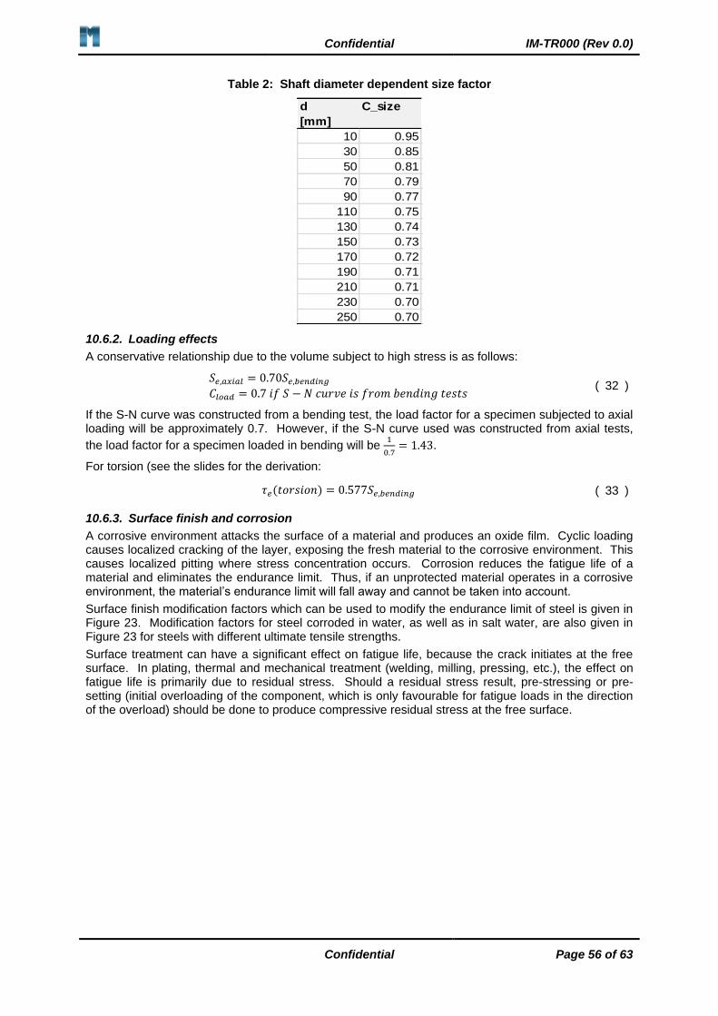
Confidential IM-TR000 (Rev 0.0)
Confidential Page 56 of 63
Table 2: Shaft diameter dependent size factor
d C_size
[mm]
10 0.95
30 0.85
50 0.81
70 0.79
90 0.77
110 0.75
130 0.74
150 0.73
170 0.72
190 0.71
210 0.71
230 0.70
250 0.70
10.6.2. Loading effects
A conservative relationship due to the volume subject to high stress is as follows:
𝑆𝑒,𝑎𝑥𝑖𝑎𝑙 = 0.70𝑆𝑒,𝑏𝑒𝑛𝑑𝑖𝑛𝑔
𝐶𝑙𝑜𝑎𝑑 = 0.7 𝑖𝑓 𝑆 − 𝑁 𝑐𝑢𝑟𝑣𝑒 𝑖𝑠 𝑓𝑟𝑜𝑚 𝑏𝑒𝑛𝑑𝑖𝑛𝑔 𝑡𝑒𝑠𝑡𝑠 ( 32 )
If the S-N curve was constructed from a bending test, the load factor for a specimen subjected to axial loading will be approximately 0.7. However, if the S-N curve used was constructed from axial tests,
the load factor for a specimen loaded in bending will be 1
0.7= 1.43.
For torsion (see the slides for the derivation:
𝜏𝑒(𝑡𝑜𝑟𝑠𝑖𝑜𝑛) = 0.577𝑆𝑒,𝑏𝑒𝑛𝑑𝑖𝑛𝑔 ( 33 )
10.6.3. Surface finish and corrosion
A corrosive environment attacks the surface of a material and produces an oxide film. Cyclic loading causes localized cracking of the layer, exposing the fresh material to the corrosive environment. This causes localized pitting where stress concentration occurs. Corrosion reduces the fatigue life of a material and eliminates the endurance limit. Thus, if an unprotected material operates in a corrosive environment, the material’s endurance limit will fall away and cannot be taken into account.
Surface finish modification factors which can be used to modify the endurance limit of steel is given in Figure 23. Modification factors for steel corroded in water, as well as in salt water, are also given in Figure 23 for steels with different ultimate tensile strengths.
Surface treatment can have a significant effect on fatigue life, because the crack initiates at the free surface. In plating, thermal and mechanical treatment (welding, milling, pressing, etc.), the effect on fatigue life is primarily due to residual stress. Should a residual stress result, pre-stressing or pre-setting (initial overloading of the component, which is only favourable for fatigue loads in the direction of the overload) should be done to produce compressive residual stress at the free surface.

Confidential IM-TR000 (Rev 0.0)
Confidential Page 57 of 63
Figure 23: Surface finish modification factors for steel (ASM International, 2008:16)
According to BS 7608 (1993), for unprotected joints exposed to water (specifically sea water) the basic S-N curves should be reduced by a factor of 2 on life for all joint classes. For high strength steels, with yield strengths of higher than 400 MPa, this factor may not be adequate and the use of such materials under corrosion fatigue conditions should be approached with caution.
10.6.3.1. Plating
Chrome and Nickel plating of steels can cause up to 60% reduction in endurance limits. High tensile stresses are generated by plating process. To alleviate residual stress problem:
• Nitride part before plating
• Shot peen part before or after plating (Best to peen after plating)
• Bake or anneal the part after plating
Corrosion resistance offered by plating can more than offset the reduction in fatigue strength seen in non-corrosive environment. Plating with cadmium and zinc appear to have no effect on fatigue strength. Electroplating can cause hydrogen embrittlement.
10.6.4. Temperature
• Diffusion processes such as carburizing and nitriding beneficial for fatigue strength
– Produces higher strength material on surface
– Causes volumetric changes that produce residual compressive stresses
• Flame and induction hardening
– Cause phase transformation which in turn cause volumetric expansion

Confidential IM-TR000 (Rev 0.0)
Confidential Page 58 of 63
– If localized to surface – compressive residual stresses result that is beneficial for fatigue strength
• Hot rolling and forging
– Cause surface decarburization
– Loss of carbon atoms from surface causes lower strength and may produce residual stresses
– Both factors are detrimental to fatigue strength
• Manufacturing processes such as grinding, welding, flame cutting etc.
– Can set up detrimental residual tensile stresses
– Shot peening effective to undo damage caused by these processes
• Endurance limits of steels increase at low temperatures (watch out for brittleness)
• Endurance limit for steels disappears at high temperatures due to mobilization of dislocations
• For T>Tmelt/2 creep becomes important
– Stress-life approach no longer applicable.
• Annealing happens at high temperatures that may remove beneficial residual compressive stresses
According to Roymech:
𝐶𝑇 =1.0 𝑓𝑜𝑟 𝑇 ≤ 450 ℃
1 − 5.8−3(𝑇 − 450), 𝑓𝑜𝑟 450 < 𝑇 ≤ 550 ℃ ( 34 )
10.6.5. Reliability
The probability of survival, or failure, is statistically driven. BS 7608 provides means to shift various S-N fatigue curves for client specified probability of survival.
10.6.6. Mechanical modifying factors
• Cold work processes – rolling & shot peening
– Produce compressive residual stresses
• Gives the greatest improvement in fatigue life
– Work-hardens the material
– Rolling cause deep stress layer (bolts, etc)
– Shot peening gives (compressive stress = 0.5Sy) layer of ~1 mm
– Shot peening:
• leaves dimpled surface: hone or polish part after shot peening
Confidential IM-TR000 (Rev 0.0)
Confidential Page 59 of 63
• Undo deleterious effects caused by chrome and nickel plating, decarburization, corrosion, grinding, etc.
• Steels with Fy ≤ 550MPa seldom cold rolled or shot peened (Easy to introduce plastic strains that wipe out residual stresses)
• Surfaces can be overpeened! Subsurface failures may occur!
• Loading frequency
– Similar data at various frequency in non-corrosive environment
– Corrosion-fatigue are greatly influenced by loading frequency
10.7. Derivation of S-N curve for S1000 and Se modified by the fatigue notch factors
From the theory presented in class, the fatigue notch factors modify the S-N curve as follows:
𝑆1000′ =
𝑆1000
𝐾𝑓′
𝑆𝑒′ =
𝑆𝑒
𝐾𝑓
( 35 )
The S-N curve is modelled by equation: 𝑆103𝑚 ×103 = 𝑆𝑒
𝑚×106. Using this relation, the coefficient and
exponent in the notch modified S-N curve equation can be solved as follows:
(𝑆1000′ )𝑚×103 = (𝑆𝑒
′ )𝑚×106
(𝑆1000
′
𝑆𝑒′
)
𝑚
= 103
𝑚 =3
log𝑆1000
′
𝑆𝑒′
( 36 )
10.8. Endurance calculation example
Problem statement:
300WA structural steel has the following material properties:
E = 206 GPa
Sy = 300MPa
Sut =450MPa
Assume a notch fatigue factor of 𝑘𝑓 = 1.7. What is the endurance limit? How many cycles to failure
at:
1. Sa= 200MPa
2. Sa= 300MPa
Assumptions:
Investmech assumed that the fatigue notch factor at 1000 cycles needs to be estimated from the material properties supplied. This information was not provided in the problem statement, but, will be inferred from the class notes.
The S-N curve can be described as: 𝑆 = 𝐶𝑁𝑏.
Solution:
Figure 24 shows the relationship of the following ration to the material ultimate tensile strength of 490 MPa (70 ksi) as approximately 0.15, from which the fatigue notch factor at 1,000 cycles is 𝐾𝑓
′ =
1.1:
𝐾𝑓′ − 1
𝐾𝑓 − 1= 0.15
𝐾𝑓′ = 0.15𝐾𝑓 + 0.85
= 0.15×1.7 + 0.85 = 1.1
( 37 )
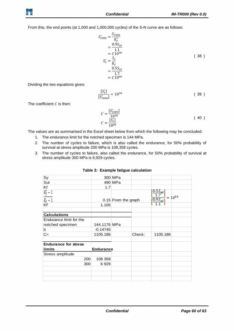
Confidential IM-TR000 (Rev 0.0)
Confidential Page 60 of 63
From this, the end points (at 1,000 and 1,000,000 cycles) of the S-N curve are as follows:
𝑆1000′ =
𝑆1000
𝐾𝑓′
=0.9𝑆𝑢𝑡
1.1
= 𝐶103𝑏
𝑆𝑒′ =
𝑆𝑒
𝐾𝑓
=0.5𝑆𝑢𝑡
1.7
= 𝐶106𝑏
( 38 )
Dividing the two equations gives:
[𝑆𝑒′ ]
[𝑆1000′ ]
= 103𝑏 ( 39 )
The coefficient 𝐶 is then:
𝐶 =[𝑆1000
′ ]
103𝑏
𝐶 =[𝑆𝑒
′ ]
106𝑏
( 40 )
The values are as summarised in the Excel sheet below from which the following may be concluded:
1. The endurance limit for the notched specimen is 144 MPa.
2. The number of cycles to failure, which is also called the endurance, for 50% probability of survival at stress amplitude 200 MPa is 108,358 cycles.
3. The number of cycles to failure, also called the endurance, for 50% probability of survival at stress amplitude 300 MPa is 6,929 cycles.
Table 3: Example fatigue calculation
Sy 300 MPa
Sut 490 MPa
Kf 1.7
0.15 From the graph
Kf' 1.105
Calculations
Endurance limit for the
notched specimen 144.1176 MPa
b -0.14745
C= 1105.186 Check: 1105.186
Endurance for stress
limits Endurance
Stress amplitude
200 108 358
300 6 929
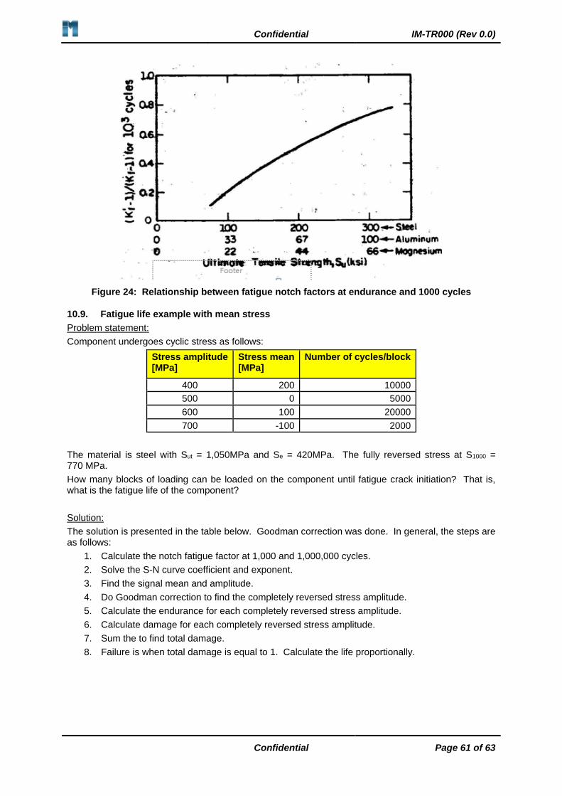
Confidential IM-TR000 (Rev 0.0)
Confidential Page 61 of 63
Figure 24: Relationship between fatigue notch factors at endurance and 1000 cycles
10.9. Fatigue life example with mean stress
Problem statement:
Component undergoes cyclic stress as follows:
Stress amplitude [MPa]
Stress mean [MPa]
Number of cycles/block
400 200 10000
500 0 5000
600 100 20000
700 -100 2000
The material is steel with Sut = 1,050MPa and Se = 420MPa. The fully reversed stress at S1000 = 770 MPa.
How many blocks of loading can be loaded on the component until fatigue crack initiation? That is, what is the fatigue life of the component?
Solution:
The solution is presented in the table below. Goodman correction was done. In general, the steps are as follows:
1. Calculate the notch fatigue factor at 1,000 and 1,000,000 cycles.
2. Solve the S-N curve coefficient and exponent.
3. Find the signal mean and amplitude.
4. Do Goodman correction to find the completely reversed stress amplitude.
5. Calculate the endurance for each completely reversed stress amplitude.
6. Calculate damage for each completely reversed stress amplitude.
7. Sum the to find total damage.
8. Failure is when total damage is equal to 1. Calculate the life proportionally.

Confidential IM-TR000 (Rev 0.0)
Confidential Page 62 of 63
Sy ?? MPa
Sut 1050 MPa
Kf 1
0.15 From the graph
Kf' 1
Calculations
S1000' 945
Size factor 1
Surface factor 1
Temperature factor 1
Reliability factor 1
Endurance limit for
the notched
specimen
525.0 MPa
b -0.085
C= 1701.0 Check: 1701
Stress amplitude Mean stress ni
Compl. Rev.
Stress Sa Ni Di
400 200 10000 494 inf 0.00
500 0 5000 500 inf 0.00
600 100 20000 663 64 218 0.31
700 -100 2000 639 99 086 0.02
Total Damage 0.33
Duration 1 Blocks
Life 3.02 Blocks
10.10. Conclusion
• Endurance limit only exist in plain carbon and low-alloy steels
• Following factors will reduce the endurance limit
– Tensile mean stress, large section size, rough surface finish, chrome and nickel plating (except in corrosive environment), decarburization due to forging and hot rolling, severe grinding
• Following factors tend to increase the endurance limit:
– Nitriding, flame and induction hardening, carburization, shot peening, cold rolling
– Chrome and nickel plating for materials in a corrosive environment

Confidential IM-TR000 (Rev 0.0)
Confidential Page 63 of 63
11. STRAIN LIFE ANALYSIS
This section introduces strain life analysis. This is for specialist application only and no notes will be issued in class. A presentation will be done just to introduce the concept to students. No assessment in assignments or examination will be done on this topic. Students may download the documents listed below for information purposes.
Presentation used in class: Investmech - Fatigue (Strain life analysis) R0.0
Download link for the Excel sheet for strain
life sequence effects:
Document name: Strain life example - Sequence
effect.xls
Link: http://www.investmech.com/fatigue.html