MSC in Finance and International Business

Author: Cagdas Ozan Ates

Academic Advisor: Paula Peare

Behavioural Finance

&

Sports Betting Markets

June – 2004

Introduction:................................................................................................................ 1 Methodology ............................................................................................................... 2

1. Development of Behavioral Finance .......................................................................... 4 1.1. A Brief History of Finance: ................................................................................. 4 1.2. Behavioral Finance Literature: .......................................................................... 11 1.3. The Causes of Anomalies: Behavioral Finance Terms...................................... 15

2. Betting....................................................................................................................... 20 2.1.1 History of Betting ............................................................................................ 21 2.1.2. Betting Terms.................................................................................................. 23 2.1.3. Betting Market Structure: ............................................................................... 27 2.1.4. Taxation: ......................................................................................................... 31 2.1.5 Customer Profile: ............................................................................................. 32 2.2. Why Do People Bet?.......................................................................................... 34 2.2.1 Psychological Reasons:.................................................................................... 34 2.2.2 Factors Behind Bettor Behavior: ..................................................................... 38 2.3 How Odds Are Set .............................................................................................. 41 2.4 Comparison between Financial Markets and Betting Markets ........................... 43 2.5. Financial Researches on Betting........................................................................ 44 2.5.1 Point Spreads and Efficiency in Betting Markets ............................................ 45 2.5.2 Favourite/Longshot Bias.................................................................................. 48 2.5.3. Asymmetric Information................................................................................. 49 2.5.4. Hot Hand Fallacy ............................................................................................ 50 2.6. Fundamentals or Noise?..................................................................................... 53 2.7. Stock Market Developments on Betting Markets: Betting Exchanges.............. 60 Conclusion ................................................................................................................ 63 References................................................................................................................. 66

1

Introduction:

Betting, found in ancient times, has been a form of entertainment for many people in

history. People like to challenge themselves on their knowledge – or luck – of predicting

the winner in games, events or contests. Betting gives an opportunity to earn money with

a proportion of the capital or lose it all; it is all or nothing. The outcomes are set prior to

the event and they depend on the result. This clarity provides researchers a controlled

laboratory test opportunity: The variables are few and the outcome is certain. In this

sense, betting provides data to test some theories related to Mathematics, Statistics and

Finance. One of the reasons that motivated me for such a research is that the controlled

laboratory environment can help to test hypotheses that can not be tested in financial

markets.

The complexity of human behavior exemplified by the gambling phenomenon has to be

taken into account in understanding the etiology of bubbles in speculative markets.

Gamblers may have very rational expectations, at some level, for the likely outcome of

their gambling, and yet have other feelings that drive their actual behavior. On the other

hand, the bias of seeing what others cannot see -and the excitement of it- may drive

investor behaviors as well. If this occurs all at once for many, it might create bubbles in

stock prices; like it did in the last decade. It is therefore important to research betting

markets and bettor behavior from an investor view.

This research is planned as a literature survey and a market research on betting markets

from a behavioral finance point of view. The paper is aimed to cover betting markets for

financial researchers and to be a guide book on these markets for scientists. My

expectation is that behavioral finance can be a tool to understand betting markets and

these markets can provide some findings for behavioral finance. The first goal of this

paper is to test the concerning expectation by analyzing the betting markets from a

behavioral finance point of view and search if finance can benefit from these markets.

A major motive to study betting is to observe the gambler behavior and learn from a

different decision making process. The similarities and differences of investor and

gambler decisions can help scientists to find clues about rational and irrational behavior.

2

Furthermore, it is aimed to make a literature survey of finance on betting markets. By this

study, I want to make a compilation of the present findings in betting markets and an

extended guide for future financial researches that have interest in this field. There is no

such study that covers all the researches in betting markets from a financial view. This

project is aimed to be the first study that gathers all financial interest in this field and a

guideline for further researches.

It is a major aim of this research to analyze betting market structure and betting industry.

By covering this alternative market, this paper is aimed to be a guide for understanding

the betting markets in detail.

Moreover, analyzing the traits and biases that motivate bettors is another major goal. The

findings may help understanding decision making under uncertainty.

Moreover, betting provides an opportunity to observe risk management. The use of

historical data, information, expert views are all in action trying to find mispriced odds.

The hedging skills must be perfect for odd makers to exist.

Furthermore, a replication of Sauer and Brown (1993) with a different data is another

goal for this paper. This replication is an important example of how tests that cannot be

done in financial markets can take place in the betting markets.

The research is mainly focused on interaction of two main components, behavioral

finance and betting markets. Besides all the goals above, this interaction will be the main

theme of the paper. The interaction is both ways: The application of behavioral finance to

betting markets and the findings in betting markets as evidence to behavioral finance

terms.

Methodology

The research is divided into 2 main parts. The first part aims to create a base on how

traditional and behavioral finance developed and a summary of key terms and findings in

this field. In the second part betting markets are researched on the basis that is built on

first part.

3

The paper starts with a brief summary in history of finance. The main theories and

developments are briefly explained. Finance history part is compiled in a way that

underlines the developments that brought behavioral finance. This paper is mainly

concerned on behavioral finance’s point of view on betting markets and therefore a base

on behavioral finance is aimed in the first part. After the Efficient Markets Hypothesis is

introduced, the birth of Behavioral Finance is explained. Behavioral Finance terms,

discussions and its alternative approach to basic finance terms are introduced. Since

Psychology is a big part of this discipline, its terms are used when in need. This base is

built in order to form a stand point for the rest of the research. This stand point underlines

that it is a financial research and it aims to have some answers, suggestions or alternative

ideas from betting markets for financial markets.

Traditional finance and behavioral finance have some areas where each side has different

opinions on. There are some topics where big discussions take place between followers of

traditional and behavioral finance (efficient markets theory, investor rationality, biases

etc.). Sports betting is researched in this paper in order to benefit from a different market

place where testing some of these topics is easier and results can be a comparison tool.

Following the first base, betting is introduced. History of betting, specific terms, market

structure and different sides of betting markets are researched. Bettor behaviors are

analyzed and the reasons to gamble are researched.

Betting firms make profits as the bettors wager for each side of the result of a game.1

With the commissions that odd makers charge the bettors, there is a secure profit in the

long run for betting companies. The question of “Given these facts why do people bet?”

is explored through this part.

After the reader gets familiar with betting and its components, a literature review in

betting markets from a financial perspective is done. There are several famous topics for

Finance researchers to conduct a study in these markets. The researches in each of them

are explained. This part gives the reader a view of what opportunities the betting markets

can bring the scientists to explore their theories in an alternative market. Following the

financial literature review, an example of an interesting empirical study, Sauer and

1 This situation is the aim of the odd maker in order to have a risk free income. It will be discussed further in the betting part.

4

Brown (1993) is explained in detail and their study is replicated with a different set of

data.

At the end of the betting part, a new market structure, betting indexes, are introduced.

This structure is inspired by stock market structure and is a perfect example of how

betting benefits from findings of finance. Bettors become investors and free market rules

start working with this new system. The research ends with a review of what can be the

next for betting markets.

1. Development of Behavioral Finance

1.1. A Brief History of Finance:

Finance theory has a surprisingly short history in economics. Economists have long been

aware of the basic economic function of credit markets but they were not keen on

analyzing it much further than that.

Irving Fisher (1906, 1907, 1930) had outlined the basic functions of credit markets for

economic activity, specifically as a way of allocating resources over time. Moreover, he

had recognized the importance of risk in the process. In developing their theories of

money, John Maynard Keynes (1930, 1936), John Hicks (1934), Nicholas Kaldor (1939)

and Jacob Marschak (1938) conceived of portfolio selection theory in which uncertainty

played an important role.

Many economists in this period didn’t have substantial researches on price

determinations. Financial markets were still regarded as mere "casinos" rather than

"markets". In their view, asset prices were determined largely by expectations and

counter-expectations of capital gains.

Big effort was spent on the topic of speculative activity (i.e. the purchase/temporary sale

of goods or assets for later resale). For instance, in their pioneering work on futures

markets, John Maynard Keynes (1923, 1930) and John Hicks (1939) argued that the

price of a futures contract for delivery of a commodity will generally be below the

5

expected spot price of that commodity (what Keynes called "normal backwardation").

This, Keynes and Hicks argued, was largely because hedgers shifted their price risk onto

speculators in return for a risk premium. Nicholas Kaldor (1939) went on to analyze the

question of whether speculation was successful in stabilizing prices and, in so doing,

expanded Keynes's theory of liquidity preference considerably. In later years, Holbrook

Working (1953, 1962) would dispute this, arguing that there was, in fact, no difference

between the motivations of hedgers and speculators. This led to an early empirical race.

Hendrik Houthakker (1957, 1961, 1968, 1969) finding evidence in favor of normal

backwardation and Lester Telser (1958, 1981) finding evidence against it.

John Burr Williams (1938) was among the first to challenge the "casino" view

economists held of financial markets and questions of asset pricing. John Burr

introduced the term intrinsic value to asset pricing. Intrinsic value, defined as the present

worth of future dividends, or of future coupons and principal, is of practical importance

to every investor because it is the critical value above which he cannot go in buying or

holding, without added risk. If a man buys a security below its investment value he need

never lose, even if its price should fall at once, because he can still hold for income and

get a return above normal on his cost price; but if he buys it above its investment value

his only hope of avoiding a loss is to sell to someone else who must in turn take the loss

in the form of insufficient income.

Harry Markowitz (1952) realized that as the "fundamentalist" notion relied on

expectations of the future, then the element of risk must come into play and thus

profitable use could be made of the newly developed expected utility theory of John von

Neumann and Oskar Morgenstern (1944). Markowitz formulated the theory of optimal

portfolio selection in the context of trade-offs between risk and return, focusing on the

idea of portfolio diversification as a method of reducing risk - and thus began what has

become known as "Modern Portfolio Theory" or simply MPT.

The idea of an optimal portfolio allocation had already been considered by Keynes, Hicks

and Kaldor in their theories of money, and thus it was a logical step for James Tobin

(1958) to add money to Markowitz's story and thus obtain the famous "two-fund

6

separation theorem". Effectively, Tobin argued that agents would diversify their savings

between a risk-free asset (money) and a single portfolio of risky assets (which would be

the same for everyone). Different attitudes towards risk, Tobin contended, would merely

result in different combinations of money and that unique portfolio of risky assets.

The Markowitz-Tobin theory was not practical. Specifically, to estimate the benefits of

diversification would require that practitioners calculate the covariance of returns

between every pair of assets. In their Capital Asset Pricing Model (CAPM), William

Sharpe (1964) and John Lintner (1965) solved this practical difficulty by demonstrating

that one could achieve the same result merely by calculating the covariance of every asset

with respect to a general market index. With the necessary calculating power reduced to

computing these less number of terms ("betas"), optimal portfolio selection became

computationally feasible.

The CAPM would however be eventually challenged empirically in a series of papers by

Richard Roll (1977, 1978). One of the alternatives offered up was the "intertemporal

CAPM" (ICAPM) of Robert Merton (1973). Merton's approach and the assumption of

rational expectations led the way to the Cox, Ingersoll and Ross (1985) partial differential

equation for asset prices and, perhaps only a step away, Robert E. Lucas's (1978) theory

of asset pricing.

A more interesting alternative was the "Arbitrage Pricing Theory" (APT) of Stephen A.

Ross (1976). Stephen Ross's APT approach moved away from the risk vs. return logic of

the CAPM, and exploited the notion of "pricing by arbitrage" to its fullest possible

extent. As Ross himself has noted, arbitrage-theoretic reasoning is not unique to his

particular theory but is in fact the underlying logic and methodology of virtually all of

finance theory. The following famous financial theorems illustrate Ross's point.

The famous theory of option pricing by Fisher Black and Myron Scholes (1973) and

Robert Merton (1973) relies heavily on the use of arbitrage reasoning. Intuitively, if the

returns from an option can be replicated by a portfolio of other assets, then the value of

the option must be equal to the value of that portfolio, or else there will be arbitrage

7

opportunities. Arbitrage logic was also used by M. Harrison and David M. Kreps (1979)

and Darrell J. Duffie and Chi-Fu Huang (1985) to value multi-period securities.

The famous Modigliani-Miller theorem (or "MM") on the irrelevance of corporate

financial structure for the value of the firm also employs arbitrage logic. This theorem

Franco Modigliani and Merton H. Miller (1958, 1963) can actually be thought as an

extension of the Separation Theorem" originally developed by Irving Fisher (1930).

Effectively, Fisher had argued that with full and efficient capital markets, the production

decision of an entrepreneur-owned firm ought to be independent of the intertemporal

consumption decision of the entrepreneur himself. In other words, the profit-maximizing

production plan of the firm will not be affected by the borrowing/lending decisions of its

owners; i.e. the production plan is independent of the financing decision.

Modigliani-Miller extended this proposition via arbitrage logic. Viewing firms as assets,

if the underlying production plans of differently-financed firms are the same, then the

market value of the firms will be the same, since there would be an arbitrage opportunity

otherwise. Consequently, arbitrage enforces that the value of the firms to be identical,

whatever the composition of the firm's financial structure is.

The second important strand of work on finance was the empirical analysis of asset

prices. A particularly interesting finding was that it seemed that prices tended to follow a

random walk. More specifically, as documented by Louis Bachelier (1900) (for

commodity prices) and later confirmed in further studies by Holbrook Working (1934)

(for a variety of price series), Alfred Cowles (1933, 1937) (for American stock prices)

and Maurice G. Kendall (1953) (for British stock and commodity prices), it seemed as

there was no correlation between successive price changes on asset markets.

The Working-Cowles-Kendall empirical findings were greeted with horror and disbelief

by economists. If prices are determined by the "forces of supply and demand", then price

changes should move in particular direction towards market clearing and not

randomly. Not everyone was displeased with these results. Many viewed them as proof

that the "fundamentalist" theory was incorrect, i.e. that financial markets really were wild

casinos and that finance was thus not a legitimate object of economic concern. Yet others

8

crowed that it proved the failure of traditional "statistical" methods to illuminate much of

anything. High-powered time series methods were used by Clive Granger and Oskar

Morgenstern (1963) and Eugene F. Fama (1965, 1970), but they came up with the same

randomness result.

The birth of Efficient Markets Hypothesis

The great breakthrough was due to Paul A. Samuelson (1965) and Benoit Mandelbrot

(1971). Far from proving that financial markets did not work according to the laws of

economics, Samuelson interpreted the Working-Cowles-Kendall findings as saying that

they worked all too well. The basic notion was simple: if price changes were not random

(and thus predictable), then any profit-hungry arbitrageur can easily make appropriate

purchases and sales of assets to exploit this. Samuelson and Mandelbrot thus posited the

celebrated "Efficient Market Hypothesis" (EMH): namely, if markets are working

properly, then all public (and, in some versions, private) information regarding an asset

will be channelled immediately into its price. If price changes seem random and not

predictable, that is since the investors are doing their jobs: all arbitrage opportunities have

already been exploited to the extent to which they can be.

The "Efficient Markets Hypothesis" was made famous by Eugene Fama (1970). It did not

please many practioners. "Technical" traders or "chartists" who believed they could

forecast asset prices by examining the patterns of price movements were confounded: the

EMH told them that they could not "beat the market" because any available information

would already be incorporated in the price.

EMH is probably one of the most resilient empirical propositions. It is unable to explain

on particular objections: for example, if all information is already contained in prices and

investors are fully rational, then not only can one not profit from using information,

indeed, there might not be any trade at all. These peculiar, contradictory implications of

rational expectations were demonstrated by Sanford J. Grossman and Joseph E. Stiglitz

(1980) and Paul Milgrom and Nancy Stokey (1982). Intuitively, the objection can be put

this way (with some oversimplifying): The efficient markets hypothesis effectively

implies that there is "no free lunch", i.e. there are no $100 bills lying on the pavement

9

because, if there were, someone would have picked them up already. Consequently, there

is no point in looking down at the pavement (especially if there is a cost to looking

down). But if everyone reasons this way, no one looks down at the pavement, and then

any $100 bills that might be lying there will not be picked up by anyone. But then there

are $100 bills lying on the pavement and one should look down. But then if everyone

realizes that, they will look down and pick up the $100 bills, and thus we return to the

first stage and argue that there are not any $100 bills (and therefore no point in looking

down, etc.) This circularity of reasoning is what makes the theoretical foundations of the

efficient markets hypothesis somewhat shaky.

Fundamental and Noise Risks:

On another main strand, researchers were arguing that some features of asset prices are

most plausibly interpreted as deviations from fundamental value, and that these

deviations are brought about by the presence of traders who are not fully rational. This

was against Friedman (1953) argument. He stated in his work that rational traders would

quickly undo any dislocations caused by irrational traders. He introduced an example

with shares of car companies as follows:

“Suppose fundamental value of a share of Ford is $20. Imagine that a group of irrational

traders become excessively pessimistic about Ford’s future prospects and through its

selling, pushes the price to $15. Defenders of the EMH argue that rational traders, sensing

an attractive opportunity, will buy the security at its bargain price and at the same time,

hedge their bet by shorting a “substitute” security, such as General Motors, that has

similar cash flows to Ford in future states of world. The buying pressure on Ford shares

will then bring their price back to fundamental value” (Friedman, 1953)

The argument against Friedman (1953) about asset prices was mainly on the ideality of

substitute securities. Barberis and Thaler (2002) summarized argument from a behavioral

finance point of view: “Even when asset is wildly mispriced, strategies designed to

correct the mispricing can be both risky and costly, rendering them unattractive. As a

result mispricing can persist unchallenged.” This case is against market efficiency and it

happens often in the financial markets. There are 2 different risks on the factors in the

determination of prices; fundamental risk and noise trader risk. Barberis and Thaler

(2002) work on the same example, Ford and GM in the car industry in order to explain

10

these risks. The most obvious risk an arbitrageur faces if he buys Ford’s stock at $15 is

that a piece of bad news about Ford’s fundamental value causes the stock to fall further,

leading to losses. This is the fundamental risk. They argue that arbitrageurs buying Ford

at $15 and shorting GM, they hedge the industry risk; however they cannot hedge the risk

of news specific to Ford Company, i.e. defective tires. They criticize that this kind of

news is also a part of the fundamental risk and this risk cannot be justified by only

hedging with a substitute stock.

“The noise trader risk is the risk that mispricing being exploited by the arbitrageur

worsens in the short run” (De Long et al, 1990a). Arbitrageurs still face the risk that the

pessimistic investors can cause Ford to be undervalued in the first place become even

more pessimistic, lowering the price even further. Noise trader risk matters because it can

force arbitrageurs to liquidate their positions early, bringing them potentially steep losses.

A clear evidence for this kind of behavior is the index inclusions. Harris and Gurel (1986)

found out when a stock is added to the index, it jumps in price by an average of 3.5%,

and much of this jump is permanent, which supports the evidence that irrationality can

persist.

Asset price volatility was researched by many scientists and tests were run in many

researches. Shiller (1979) stated that both bond and stock prices are far more volatile

than can be justified on the basis of real economic events. Arrow (1982) suggests that

psychological models of irrational decision making of the type suggested by Tversky and

Kahneman (1981) can help to explain behavior in speculative markets. There are many

behavioral finance followers defending that existing evidence does not establish that

financial markets are efficient in the sense of rationality reflecting fundamentals. On the

other hand some researchers still point to the inability of professional money managers to

beat the market as strong evidence of market efficiency.2

With these critics of efficient markets hypothesis, behavioral finance was born. It

basically defends that investors can be irrational; prices might not reflect all information

and markets can be wrong.

2 Rubinstein, 2000, Ross, 2001

11

At this point, it should be stated that it is really hard to distinguish the noise and

fundamental components in price volatility on assets in financial markets. In many cases,

it is too complicated to determine which risk causes the price changes and it is hard to

interpret them for taking positions. My paper is going to continue analyzing components

of asset prices in section 2.6 in a different environment, where fundamental and noise

components of asset prices will be discussed in betting markets. A replication study of

Sauer and Brown (1993), analyzing fundamental and noise component in betting markets

can be seen in the concerning section.

By the efficient markets hypothesis was being discussed in financial era, an alternative

approach evolved. This alternative way is one of the main topics of this paper, namely,

Behavioral Finance.

1.2. Behavioral Finance Literature:

“Behavioral finance is the application of psychology to financial behavior”(Shefrin,

2002).

Behavioral Finance has been a popular term in the finance literature since the 80’s.

Especially by bringing its own explanations on “anomalies” like the eastern markets

crush and bubbles of technology stocks, behavioral finance gained more attention.

The main starting point for Behavioral finance was from psychologists. They pointed out

imperfections of the investor decisions, inefficiency in markets and heuristics and biases3

of human nature.

“In the 80s, scholars began to discover a host of empirical results that were not consistent

with the CAPM and efficient markets theory. Proponents of traditional finance regarded

these findings as anomalous, and thus called them anomalies. The anomalies started with

size –e.g. the small-firm effect- and kept on coming. Soon there was January effect, the

weekend effect, and the holiday effect. As they discovered new anomalies, scholars

began to wonder whether traditional finance was incapable of explaining what determines

security prices” (Shefrin, 2002).

3 See Behavioral Finance terms, page 15

12

Starting as a critic of EMH, behavioral finance developed an alternative way of

explaining financial markets. There were new terms and alternative approaches to the

traditional finance and especially to the efficient markets model.

Robert Weintraub (1963) collected the skepticism and concerns about random walk

hypothesis. He showed evidence that speculative prices do follow a trend. He also stated

an interesting argument; the “seats” of floor traders on the NYSE, licenses to speculate

where trades are executed, can often be sold for thousands of dollars (presently millions

of dollars). Why would it be this expensive to have a seat in there if there were no price

patterns? He states that these men earn their incomes by betting against the applicability

of the random walk hypothesis to price moves.

Paul Samuelson (1963) covered risk and uncertainty from an alternative view. He applied

the law of large numbers of James Bernoulli to insurance companies. He researched if

insurance companies can reduce their risk by increasing the number of ships it insures.

He found out that the correct relation is hedging by subdividing the ownership on the

ships. He also concluded that a person whose utility schedule prevents him from ever

taking a specific favorable bet when offered only once can never rationally take a large

sequence of such fair bets, even if expected utility is maximized.

Niederhoffer (1966) pointed out the importance of psychology of investors and its effect

on market. He underlined what previously Osborne found. Investors prefer trading on

even eights rather than prices ending in odd eights. Having a psychological reason, he

concluded that this is against random walk hypothesis.

Moreover, Stevenson and Bear (1970) found evidence on speculative price movements

on commodity future prices do move in a systematic, as opposed to a random, manner.

Miller (1977) found contradictions in investor behaviors against EMH. He stated that it is

implausible to assume that although future is very uncertain, and forecasts are very

difficult to make, somehow everyone makes identical estimates of the return and risk

from every security. In practice, the very concept of uncertainty implies that reasonable

men may differ in their forecasts.

It wouldn’t be exaggerating to say that Amos Tversky and Daniel Kahneman have made

the pioneer researches in the area and they could be named as the inventors of Behavioral

Finance. They introduced the heuristic-driven errors to finance in their first article,

13

Judgement under uncertainty: Heuristics and biases (1974). Moreover they explained a

new term to financial markets, frame dependence (1979). They formed up an alternative

theory to expected utility theory and called it as prospect theory. They concluded that

people behave in many ways that systematically violate the axioms of rational behavior

under uncertainty. These findings along with some others were turned into a guide book

for behavioral finance followers (Judgment under uncertainty: Heuristics and biases,

1982). On a book review, another famous scientist, Richard Thaler, stated the following

words for this work: “The papers chosen for this book are an excellent collection,

generally well-written and fascinating.”4This book is still one of the most referred sources

in the field.Furthermore, many studies were inspired by prospect theory. Loomes and

Sugden (1982) made a simpler alternative to this theory and named it as regret theory.5

In July 1985, The Journal of Finance gathered attention to behavioral finance by

publishing two papers from this field. First paper, by Werner De Bondt and Richard

Thaler, applied Tversky and Kahneman’s notion of representativeness6 to market pricing.

De Bondt and Thaler (1985) argued that investors overreact to both bad news and good

news. Therefore, overreaction leads past losers to become underpriced and past winners

to become overpriced. The second paper, by Meir Statman and Shefrin, applied

Kahneman and Tversky’s notion of framing to the realization of losses. They called this

phenomenon as the disposition effect, arguing that investors are predisposed to holding

losers too long and selling winners too early. These two papers were among the first ones

to point out that the irrationality can be general in the markets. They were referred by

many further researches.

Keim (1983) found empirical evidence that for the period 1963 to 1969 positive returns to

small firms during the first week of Janunary was unexpectedly large. This was called the

turn of the year effect - or January effect. Roll (1983) worked on the same topic with a

different time period and found consistent results on the turn of the year effect.7 De Bondt

and Thaler (1985) shed new light on the January returns by researching the returns earned 4 Thaler, R. , book review, Journal of Economic Literature, Vol. xxi, sept. 1983, pp: 1048 5 LOOMES, Graham and Robert SUGDEN, “Regret Theory: An Alternative Theory of Rational Choice Under Uncertainty”, The Economic Journal, Volume 92, Issue 368 (Dec., 1982), 805-824. 6 See Behavioral Finance terms, page 15 7 Roll, R. , Journal of Portfolio Management, “The turn of the year effect and the return of the premia of small firms”, 1983, 18-28

14

by prior "winners" and "losers." They found empirical evidence that portfolios of losers

experienced exceptionally large January returns as late as five years after portfolio

formation. They stated that their data is consistent with the researches in experimental

psychology: Most people tend to overreact to unexpected dramatic news events.

Fischer Black (1986) introduced the term noise trading in the markets. He stated that

trading on noise as if it was information, must be a significant factor in the securities

markets. “Noise, in the sense of a large number of small events, is often a casual factor

much more powerful than a small number of large events can be. Noise causes markets to

be somewhat inefficient, but often prevents us from taking advantage of inefficiencies”.

(Black, 1986)

Trueman (1988) provided evidence that the incentive for a manager to engage in noise

trading arises because of the positive signal that the level of manager’s trading provides

about his or her ability to collect private information concerning current and potential

investments. Thereby another irrational behavior was found.

The efforts to adjust behavioral finance terms to decision making process have produced

many interesting researches.

Heath and Tversky (1991) modified ambiguity aversion8, a term introduced by Savage

(1964). They argued that in the real world, ambiguity aversion has much to do with how

competent an individual feels he is at assessing the relevant distribution.

Andrew Lo (1999) tried implementing Behavioral Finance in Financial Risk

Management.9 Beginning with behavioral issues in risk management, Lo introduced his

three P’s.: Prices (meaning the cost of reducing risk, by hedging for example), Probability

(the chance of loss) and Preferences (how much risk to hedge). The analytic models in

finance focus on the first two, and say little or nothing about the level of risk that is

appropriate. The challenge for risk management is to integrate the three P’s into a single

and complete risk management protocol. Lo concludes that in order to find this protocol,

one has to combine different sciences: “Economics and Finance, Statistics, Biology and

the brain and cognitive sciences, may be a manifestation of the notion of consilience.”

Consilience was described by Wilson (1998) as “jumping together of knowledge by the

8 See Behavioral Finance terns, page 15 9 Lo, A., “The Three P's of Total Risk Management”, Financial Analysts Journal 55(1999), 13-26.

15

linking of facts and fact based theory across disciplines to create a common groundwork

of explanation.”

It is aimed that Behavioral Finance would be adjusted to betting markets in the same way

in order to understand these markets fully. “Consilience” is a need in this field, as it will

be discussed further in this paper.

1.3. The Causes of Anomalies: Behavioral Finance Terms

Many of the anomalies in the markets were explained with irrationality of investors. The

patterns that brought the anomalies were related to psychology. Therefore, the terms in

the Behavioral Finance are mostly from Psychology rather than Economy. These terms

can be hard to understand by just theoretical explanation; therefore an example for each

term is given in the following.

Heuristic-driven bias is one of the main reasons for irrationality. It was introduced to

Finance by Tversky and Kahnemann. Heuristic is defined as the process by which people

find things out for themselves, usually by trial and error. These trials and errors lead

people to develop some rules of thumb. Heuristics are said to be these rules of thumb.

Heuristics are quite useful, but sometimes can lead the person to errors (biases) since it

depends on the experiences.

“For example, the apparent distance of an object is determined in part by its clarity. The

more sharply the object is seen, the closer it appears to be. This rule has some validity,

because in any given scene the more distant objects are seen less sharply than nearer

objects. However the reliance on this rule leads to systematic errors in the estimation of

distance. Specifically, distances are often overestimated when visibility is poor because

the contours of objects are blurred. On the other hand, distances are often underestimated

when visibility is good because the objects are seen more sharply. Thus, heuristic of

reliance on clarity as an indication of distance leads to common biases”(Tversky-

Kahneman, 1974). Such biases are also found in the intuitive judgment of probability

which will be used in the following parts of this paper in understanding the gambler’s

behavior.

16

Another important term used in behavioral finance is known as representativeness.

Representativeness refers to judgments based on stereotypes. People make assessments of

the things they see and try to put them into groups. This grouping relies on stereotypes.

These assessments depend on the representativeness of each thing to the observer.

One of the most famous representativeness examples is the law of small numbers or

gamblers fallacy. People expect that a sequence of events generated by a random process

will represent the essential characteristics of that process, even when the sequence is

short. After observing a long run of red on the roulette wheel, for example, most people

erroneously believe that black is now due, presumably because the occurrence of black

will result in a more representative sequence than the occurrence of an additional red. The

same sequence is observed on tossing coin, i.e. expectation of head after 5 straight tails.

Even after 5 straight tails, probability is still 50-50 for heads and tails in a new toss.

Chance is commonly viewed as a self corrective process in which a deviation in one

direction induces a deviation in the opposite direction to restore the equilibrium. In fact,

deviations are not “corrected” as a chance process unfolds, they are merely diluted.10

There are situations in which people assess the frequency of a class or the probability of

an event by ease with which instances or occurrences can be brought to mind. This

judgmental heuristic is called availability. It is a useful clue for assessing frequency or

probability, since instances of large classes are usually reached better and faster than

instances of less frequent classes. However, the reliance on availability leads to

predictable biases. People can have a narrow availability, thus have wrong reasoning and

wrong results based on this availability.

To help adjusting the terms, an example from betting markets can help us to understand

availability. Biases based on availability are common in sports betting. The odds change

with new information like doubtful injuries, player transactions and news about the

teams. The gamblers that don’t have the access to this information can miscalculate the

probabilities. This bias is caused by the availability of the information to the gambler. It

is more valid in financial markets; i.e. inside traders have a better view of the company

10 Tversky A., Kahneman D., Judgment under uncertainty, Science, 1974, 185, p:1124-1131

17

than many other investors if the markets are not strongly efficient. Asymmetric

information in betting markets will further be discussed in betting markets.

Anchoring is another term used commonly in behavioral finance. In many situations

people make estimates by starting from an initial value that is adjusted to yield the final

answer. The initial value, or starting point, may be suggested by the formulation of the

problem or it may be the result of a partial computation. In either case, adjustments are

typically insufficient.11 Different starting points yield different estimates, which are

biased toward the initial values. This process is called anchoring.

There is an interesting example of this process as follows. “Two groups of high school

students estimated within 5 seconds, a numerical expression that was written on the

blackboard. One group estimated the product

8 x 7 x 6 x 5 x 4 x 3 x 2 x 1

while the other group estimated the product

1 x 2 x 3 x 4 x 5 x 6 x 7 x 8

To rapidly answer such questions, people may perform a few steps of computation and

estimate the product by extrapolation or adjustment. Because adjustments are typically

insufficient this procedure should lead to underestimation. Furthermore, because the

result of the first few steps of multiplication is higher in the descending sequence than in

the ascending sequence, the former sequence should be judged larger than the latter. Both

predictions were confirmed. The median estimate for the ascending sequence was 512,

while the median estimate for the descending sequence was 2250. The correct answer is

40320.” (Tversky-Kahneman, 1974)

Loss aversion is also one of the key terms in behavioral finance. Kahneman and Tversky

find that sunk costs have about 2½ times the impact of a gain of the same magnitude.

Many investors don’t want to give up the hope of making money on a particular

investment, or perhaps they want to get even before they get out.12 People basically don’t

like loosing and hate to accept it. This phenomenon is called loss aversion.

11 Slovic, P. & Lichtenstein S., 1971, Comparison of Bayesian and regression approaches to the study of information processing in judgment, Organizational Behavior and Human Resources, 6, 649-744 12 Gross, L., 1985, The art of selling intangibles: How to make your million by investing other people’s money, Prentice Hall

18

Kahneman-Tversky (1974) had a survey example to explain this concept. Subjects were

asked:

In addition to whatever you own, you have been given 1000. Now choose between

A= (1000, 0.5)

B= (500, 1)

B was the more popular choice. The same subjects were then asked:

In addition to whatever you own, you have been given 2000. Now choose between

C= (-1000, 0.5)

D= ( -500, 1)

This time, C was the popular choice.

Two problems are identical in terms of their final wealth positions and yet people choose

differently. Subjects focus only on gains and losses. People are risk averse over gains and

risk taking over losses (loss averse).

Conservatism is another bias practiced by investors. There are situations where base rates

are over-emphasized relative to the sample evidence. Edwards (1986) run an experiment

where there are two urns, one containing 3 blue balls and 7 red ones, and the other

containing 7 blue balls and 3 red ones. A random draw of 12 balls, with replacement,

from one of the urns yields 8 reds and 4 blues. What is the probability the draw was made

from the first urn? While the correct answer is 0.97, most people estimate a number

around 0.7, apparently overweighting the base rate of 0.5.

“At first sight, the evidence of conservatism appears at odds with representativeness.

However, there may be a natural way in which they fit together. It appears that if a data

sample is representative of an underlying model, then people overweigh the data.

However, if the data is not representative of any salient model, people react too little to

the data and rely too much on their priors” (Barberis-Thaler, 2002). In Edwards’

experiment, the draw of 8 red and 4 blue balls is not particularly representative of either

urn, possibly leading to an over reliance on prior information.

Traditional finance is aware of irrational human behaviors. However traditional finance

followers defend that people, through repetition will learn their way out of biases;

Experts in a field, such as dealers in an investment consultancy firm, will make fewer

errors and with more powerful incentives, the effects will disappear.

19

While these factors can attenuate biases to some extent, there is little evidence that they

will wipe them out altogether. The effect of learning is often muted by errors of

application: when the bias is explained, people often understand it, but then immediately

proceed to violate it again in specific applications. Expertise, on the other hand, is often a

hindrance rather than a help: experts, armed with their sophisticated models, have been

found to exhibit more overconfidence than laymen, particularly when they receive only

limited feedback about their predictions. Finally, Camerer and Hogarth (1999) find out

that while incentives can sometimes reduce the biases people display, no replicated study

has made rationality violations disappear purely by raising incentives.

The biases above are a part of almost every decision making procedure. It is the task of

every investor to adjust ways to prevent biases. Arnold S. Wood, President and CEO of

Martingale Asset Management, gives a generic prescription for bias prevention as

follows:

• Always ask what you don’t know that you need to know when making a decision

• Give your full attention to contrary opinion, i.e. encourage it

• Document decisions so hindsight bias doesn’t distort original intentions.

• Don’t confuse competence with chance over short period

This set of principals is basically a result of experience and is an example of how

investors use reminders to prevent biases.

As stated in the introduction, one of the main purposes of this study is to understand the

findings of behavioral finance within betting markets. The terms used in behavioral

finance literature is so valuable to explaining gambler behaviors that it is almost

impossible to understand these behaviors without them. The terms explained above

prepares a basis for understanding the bettor behavior in betting markets. While exploring

the gamblers world, one would often face with many of the irrational anomalies

explained. Some of them (overconfidence, wishful thinking), as we will see, can even be

seen as the reason why these markets exist.

20

2. Betting 2.1. Gambling and Introduction to betting There are different definitions in the literature for gambling. Some of them are as follows.

• Risking money in order to win money on an outcome that is wholly or partly

determined by chance (Walker, 1992)

• Wagering of valuables on events of uncertain outcome (Devereux, 1968)

• Staking money on events driven by chance (New Zealand Productivity

Commission, 1998).

Gambling is a term that covers betting while betting is used for gambling activities which

does not contain only pure luck. For example staking money on sports games is a form of

betting, while staking money on a roulette machine is not (Both of these activities are a

type of gambling but sports betting is justified by sports knowledge of bettor).

While there appears to be general agreement about what constitutes gambling, all of the

above definitions are unsatisfactory in that they also include other moderate to high-risk

activities. Starting a new business or investing on the stock market, for example, could be

included. However, most people do not regard these activities as gambling because while

the outcome of these activities may involve chance, they are not specifically designed to

part investors and their money. Gambling, as it is typically considered in science,

industry and public discourse, is presented as a form of entertainment or recreation. In

addition, consideration is usually confined to those activities that are widely perceived as

gambling and/or are defined as such by statute or for taxation and regulatory purposes.

Gambling covers all the games that people pay to participate and have a chance to get

more money in return. Lotteries, bets on sports results, bingo etc. is all under the term

gambling. In this sense, gambling also covers betting. However this study is only

specializes on sports betting. To make the distinction clear, when the term betting is used,

the sports betting is meant.

Gambling comes in many forms and takes place in a variety of social settings such as

retail outlets, hotels, clubs, casinos, race-tracks and, increasingly at home via the

21

telephone, television and Internet. It involves real money and real risks of winning and

losing. It is undertaken by a wide diversity of people with varying attitudes and

experience related to betting. Walker (1992) cautions researchers on the field: “…there is

a great danger that studies conducted with students in simulated gambling environments

for bogus money, small prizes, or course credit, will yield nothing of relevance to the real

gambling of genuine gamblers in their natural environments”. However, my paper aims

to see the market as a whole and observe all kinds of bettor behavior in order to track

clues for behavioral finance. To understand their rationale could lead us to the rationale

of investors.

2.1.1 History of Betting

Before going further with the tracking the clues of behavioral finance in betting, one

should get familiar with this market. There is a time that built up the professional sports

betting that goes back to very early times in forms of basic gambling. Gambling is an

ancient form of recreation. There is archaeological and historical evidence of gambling in

many ancient civilizations including those of the Egyptians, Chinese, Japanese, Hindus,

Persians, Hebrews and Huns13. “Gambling has been widely documented in prehistoric

cultures as well as among indigenous tribal peoples” (Gabriel, 1996). From these

accounts it is likely that Gambling emerged independently in a number of different

societies. In addition, gambling innovations and practices have been widely transported

across geographical and cultural boundaries.

Gambling appears to have been widespread throughout Europe and Asia in the Middle

Ages. “In England, by the Sixteenth Century, gambling was common place through all

social strata. Both men and women participated. Although tolerated amongst the

aristocracy and upper classes, legal measures were introduced during the early part of the

Seventeenth Century to curb gambling excesses in the lower classes. Legislation was

passed making gambling illegal for commoners except at Christmas time. Betting clubs

and houses proliferated. George II established the first national lottery. Betting on horse

races and most other sporting events became popular.” (Volberg, 1999)

13 Volberg, R., Gambling and Problem gambling in Louisiana, Gemini Research Ltd., 1999

22

The rise of the Protestant work ethic during the early part of the Nineteenth Century was

associated with a further period of betting restriction throughout much of Europe. In

England, casinos were closed; gambling laws introduced and the state lottery was

abolished in 1826. Bear-baiting and rat, dog and cock-fighting were prohibited. However,

the new laws were enforced in a discriminatory manner. Upper class gambling continued

to be condoned and flourished. Working class gambling went underground (Grant, 1994).

The first lotteries for prizes probably took place in Italy in the Middle Ages and were

brought to France and England in the mid-1500s (Clotfelter & Cook, 1989). In

revolutionary France, the glittering Palais Royal served as a tourist centre with shops and

cafes as well as over 100 illicit gambling operations featuring dice and card games.

Although the five main clubs were legalized by Napoleon in 1806, anti gambling forces

were able to compel the clubs to close in 1837. The Napoleonic laws legalizing casino

gambling formed the basis for legal gambling casinos today in France (Barnhart, 1992).

France was the first European country to reintroduce casinos at spas and resorts at the

beginning of the Twentieth Century.

It is impossible to tell just when the first sports gambling started. It seems from the

records that horse racing is one of the oldest forms of sports betting. It has started in

England in 17th century and spread to other countries. However, the professional sports

betting is valid since the sports became professional in the beginning of 20th century.

The main continents for Sports betting have been US and Europe for a long time. In the

first years the casinos were the only places where people could bet on sports events.

Television broadcasting helped the sports betting to spread faster. The rise of professional

sports, especially televised professional sports, has brought significant increases in the

volume of sports betting in the United States. Moreover, legalized sports wagering in

Nevada flourished considerably when the federal gambling tax was gradually reduced

from 10 percent to 2 percent from 1975 to 1979. The sports handle14 in Nevada increased

dramatically from less than $41 million in 1973 to almost $258.7 million by 1979. 15 This

14 see glossary for “handle” 15 The numbers are available from the website, www.delugeonline.com

23

figure is around $2 billion dollars per year now and gives an idea of how sports betting

grew in years16.

The Internet has been another milestone for sports betting firms. Now most of the

companies have an online department and almost everyone over 18 years old can have an

account from all over the world. This brought a big impact on state taxes on betting.

Some countries announced that they would not get any taxes on betting, and therefore

many companies located their base to these countries (offshore). In other words, the

Internet provided gambling a tax free location.

2.1.2. Betting Terms

There are many specific terms that are used in betting markets. A brief introduction of the

terms related with this research is summarized below. For further explanations, a betting

glossary can be found at the Appendix A of this research. The following part explains the

terms in order to understand the concept of betting.

Odds: American or European?

An odd means the betting fraction, the return of money offered for each unit bet. Odd

maker (bookmaker, bookie, or wager) is the person who offers the odds. There are two

different ways of stating an odd; American or European. There is another type of betting

called Pari-mutuel betting, where the odd is hidden (-not shown to the bettors) until the

game starts. This type of betting will be introduced at the end of this part.

American odds are shown fractionally and do not include the capital involved. An

American odd of 10/11 means that the odd maker gives $10 for every $11 if the bet is

won. European odd on the other hand is shown on decimals and includes the capital. The

same odd would be 1.91 (1 + 10/11) in terms of European odds. While the American

odds state the profit, European odds state the total income. A European odd always seem

higher to bettor since it includes capital. This can create a psychological effect on bettors:

Since the capital is included in the odd, all numbers are bigger than 1, and misleads the

bettor causing the income to seem bigger. Assume that an American odd for a team to

win is 1/1. European version of this odd is 2. It is like stating the same truth with different

16 Congressional Report, (2002)

24

sentences: in terms of American odds one would say “you invest $1 and make $1 profit if

you win” while it would be stated as “you double your money if you win” in terms of

European odds. The odds used in this research are European. American odds will not be

used hereafter.

The odds set on the different odd makers generally hold single-price principle, meaning

that all the odd makers offer usually the same odds for same games. Especially after

usage of internet became common, people can have different betting accounts on

hundreds of different companies. If there was a difference between the odds, then bettors

could take advantage of arbitrage opportunities of different prices. Therefore many book

makers do not set odds for some games before seeing market price. In fact, there seems to

be an information network between odd makers around the world.

There are several types of odds set by the odd makers; the main types are point spreads,

single odds, over-under. Moreover, some odd makers find some special bets and offer

their clients but these are not in interests of this paper.

Point spread market is one of the most common research fields in betting. Point spread is

valid mostly in American centered sports leagues like NBA, NCAA, NFL and NHL.

Point spreads, like prices in financial markets, can be viewed both as market clearing

prices and predictions of outcomes. The outcome of interest here is the score of the game,

more precisely, the difference in points by two teams. Suppose that L.A. Lakers are

hosting Chicago Bulls and that the wagering market clears with a point spread which

favors the Lakers by 11 points. This means that bets on Lakers are winners only if the

Lakers win by more than 11 points. Similarly, bets on the Lakers lose if Bulls either wins,

or lose by less than 11 points. If Lakers win by 11 points all bettors get their money back

and this is called a void bet.

The traditional sports betting companies serve odds to bettors in a way that they represent

the risk and in the long run leave a commission to the company. Most of the odd makers

in sports betting aim a commission over all bets. One can see this best on point spread

betting since they are claimed to have equal probabilities on both sides. We can work on

the same example of Los Angeles Lakers-Chicago Bulls game. The point spread (two

teams’ score margin) was announced as 11 points by the odd makers, making the two

sides equally probable. This means that odd makers think that this game will finish by 11

25

points in favor of Lakers and given the abilities of the two teams, there is no profit

opportunity by betting on whether they will score more or less than 11 points margin. The

odd makers offer odds of 1.91 for both sides of the spread, meaning that they pay 91%

profit and the capital back for the winner party. This 91% is called pay out share. The

loser party loses the capital invested. There can be more bettors positioned in one side of

the point spread causing the company loss in some single events, but in the long run the

odd makers secure their 9.89% (=(1/.91) -1) profit by offering odds at 1.91. In case of

unbalanced positions on a side, some odd makers attract the weak part by offering higher

odd or decreasing the heavy part’s odd. Some take positions by announcing different

spreads like making the spread bigger for the favorite team in order to attract bettors to

the long-shot (short side). The knowledge of the odd maker on the game to set the odd for

point spread is crucial. In order to make the betting markets an efficient one; this spread

should give the bettors the most probable result, making the bet a 50-50 choice to take

positions on one side.

The single odds on the other hand are set by the odd makers according to the probabilities

of the teams to win the game. The odds are set by dedicated probability. If we use the

same example, the return offered for Lakers to win would be less than for Chicago to

win. Assume that the odd makers profit margin is set on 9.89 percent, thus pay out share

is 91%. In order to find the odds, the odd maker appoints probabilities first. Assume that

odd maker thinks there is a probability of 75% for Lakers to win while 25% for Bulls.

The odds are set as follows:

Odd for Lakers = Pay out share / Probability of Lakers to win

Odd for Bulls = Pay out share / Probability of Bulls to win

Odd for Lakers17 = 91% / 75% = 1.21

Odd for Bulls17 = 91% / 25% = 3.64

Thus, Lakers odd offers 21% profit to bettors in case of victory while Bulls odd offers

264% profit. By offering the odds this way, the betting companies balances the money

17 Note that the odds are European.

26

invested on each side maximizing their profit. In the long run, they secure their

commission.

Under/Over bets are set for the total score of the game and usually consist of 2 same odd

on each side. Likewise in point-spread odds, in an efficient market, an under-over total

score would be the predictor of the real result.

A major and one of the oldest types of betting is pari-mutuel betting. According to the

system, the holders of winning tickets divide the total amount of money bet on a race (the

pool), after deductions for tax and racetrack expenses. The uniqueness of pari-mutuel

betting lies in the fact that the gambling public itself determines the payoff odds (e.g., if

many people have bet on the actual winner of a contest then the payoff will be low,

simply because many winners will divide the pool). In pari-mutuel betting, a

predetermined percentage is taken out of the betting pool to cover the cost of market-

maker and the remainder is returned to winning bettors in proportion to their winning

stake.

The origin of the pari-mutuel system lies in horse-race betting. “In 1865, a Frenchman

named Pierre Oller, in reaction to losing too much of his own money to the odd makers,

developed a wagering system which dispenses with odds makers who use their judgment

to decide how much a given wager should pay” (Koessler, F. , Broihanne, M. H. &

Ziegelmeyer, A., 2003). He called his system “parier mutuel", meaning mutuel stake or

"betting among ourselves." When the system was adopted in England, it became known

as “Paris mutuals" and then “pari-mutuels." Nowadays pari-mutuel wagering is the

accepted betting procedure at major horse-racing tracks throughout the world; it is

exclusively used by racetracks in North America, France, Hong Kong, and Japan and it

coexists with a bookmaking market in Australia and Great Britain. In these pari-mutuel

gambling systems, if the horse chosen by an individual wins, then his investment yields

returns (calculated through final betting odds) that are decreasing with the proportion of

bettors who have bet on the same horse. Besides, the proportion of the money in the win

pool that is bet on any given horse is interpreted as the subjective probability that this

horse will win the race and it corresponds to the implicit price of one unit of money bet.

27

2.1.3. Betting Market Structure:

Gambling is a large-scale business in 21st century. Data sourced from National Gambling

Impact Study report (1999) estimate that people spend around $380 billion annually in

one form of gambling in USA.18 Gambling on sporting events involves large amount of

money, but just how large may be impossible to determine, because a large part of sports

betting is still done illegally.

Sports betting is legal in many countries and only in Nevada in USA. Gambling was

banned by US Congress in 2002, and the reason was announced as “to protect American

youth from addiction and bad habits”. Since then, it is forbidden to use credit cards on the

internet for gambling purposes in US. Many people think that there were Las Vegas odd

makers behind the ban, who were losing their share to companies overseas. However,

people find ways to get around this law by transferring money in offshore countries.

Online sports betting is developing as the users get familiar with the internet and

overcome the security issues online. It grew further despite the bans in 2002 as

worldwide revenues topped $4 billion for that year.19 Of that amount, over $2 billion was

wagered by US residents. Bear Stearns, investment bank, backed up these findings by

estimating that the worldwide market would have been in excess of $5 billion had many

American credit card providers not discontinued offering transfers to offshore sports

books. Meanwhile, the total money wagered in Nevada on sports books (handle) was less

than $2 billion in 2002; this was the first time in a decade that the Nevada handle dropped

below $2 billion.

The Congressional Report (2002) states that the tremendous growth of both legal and

illegal betting is expected to continue into upcoming years both in US and other

countries. It is predicted by this report that the future growth of the online gaming

industry will come more rapidly on a worldwide basis than in the United States.

Americans, which now represent half of the online gaming revenues, are projected to be

only 24% of the $14.5 billion worldwide market anticipated in 2006. Japan is of extreme

18 It is very hard to find the exact figures for these markets since most of the companies keep this kind of information confidential. The most dependable research is National Gambling Impact Study which was published in 1999 by University of Chicago. 19 US Congressional Report, US General Accounting Office, December 2002

28

interest to the industry because its household internet penetration of greater than 80% is

the largest in the world and it is a country nearly as obsessed with sports as America is.

Countries with even more long-term promise for the industry are China and Malaysia

where already two times more people have gambled on the internet than have purchased a

product online.20

While international markets clearly offer an opportunity for expansion, the offshore

industry can continue to attract more new players to the industry in all countries if it

satisfies new player concerns. According to the River City Group, the primary concerns

of potential new players include: a hassle free experience; quick payments; easy

instructions; attractive web sites; easy registration; secure credit card transactions;

certificates from consumer protection agencies; better odds; ability to play for free; 24/7

customer service.21

Since the first internet gaming sites began appearing in 1995, 73 governments have

approved some form of internet gambling. The industry has grown to 1400 gambling sites

(Balestra, 2004). However, most of these sites are fairly small and cannot live for long

because of intense rivalry. There are many sites closing their operations recently because

of this rivalry.

Odds making is a money intense business. Firms must have enough liquid to balance the

bets and afford losses in single events. Betting firms can be seen as risk management

firms, hedging their risk of loss to each side. The odd maker is simply a middleman who

operates on a small - middle profit margin and, ideally, likes to see half the money

wagered on one team, and half on the other, assuring him of a profit. If too much money

is wagered on one team, the odd maker will move the line, or point spread, to encourage

bets on the other team thus enabling him to balance his book. A fair odd would create

equal amount of money on each side, but firms have to track the bets and change the odds

in case of imbalance, new information or speculations. Some firms even serve different

odds to different customers because of hedging purposes. The reasons vary for this kind

of price discrimination. For example, national games usually create overconfidence on

national team and odd makers discriminate their prices in different parts of the world.

20 US Congressional Report, US General Accounting Office, December 2002 21 Balestra, M., “Internet Gambling Report”, River City Group, 2004

29

Moreover, some skilled bettors are forbidden to wager more than some limit in order to

prevent large losses. A further discussion of how odds are set is discussed on section 2.3.

The profit that odd makers earn from the commissions is fairly small. It is between 3 to 5

percent of all the money wagered. It is said to be the only profit source of oddmakers,

however Strumpf (2003) finds that odd makers gamble and take positions on games, and

raise their profit by their knowledge. The most possible reason is the rivalry in the

market. The commissions got lower in order to attract customer making the war on

market share very intense for companies. Odd makers try decreasing the costs and

internet has helped a lot on it. Now that almost everything is online, the wagers have

lower cost. Many of them try building brand by heavy advertising and giving special

offers. However, in many countries people still prefer betting by cash in small shops.

Therefore, there is still a substantial amount of cost related with rent, employment and

paper for the companies who targets this group. Big companies who have this kind of

organization reasonably charge with higher commission rates. The following statement is

taken from an advertisement of William Hill, one of the biggest odd makers in England:

Founded in 1934, we have over 65 years' experience of offering betting services.

Currently we operate over 1,500 licensed betting offices in the UK. We have over

300,000 telephone clients worldwide, making us the world's largest telephone betting

organisation.

We employ over 9,000 people to ensure that we offer a customer experience that is

second to none. With a yearly turnover in excess of US $2.5 billion, you can rest assured

that in placing a bet with us you are wagering in a totally safe, legal and confidential

environment.

Reasonably, William Hill charges higher commission because of this type of big

organization. They offer 1.83 for point-spreads where others offer usually around 1.91

(10 for 11). This means that William Hill charges a commission of almost 2 times the

others’. The same type of organization can be seen in Dansk Tipstjeneste, where

company has licensed offices in Denmark and serve lower odds for local games

compared to the international internet sites. The customers accept lower odds because of

trademark: They know the brand and trust the odd maker. They assure that their credit

card information is not stolen. People are reluctant to spend money on the internet

30

because of their security concerns. The rumor about credit cards to be stolen over the

internet is basically the biggest reason why people do not prefer internet betting. Using

trust as a strategy is typical by the old firms that were in the business before Internet.

However, this trust problem against internet seems to dissolve and people shop more and

more on the internet. Therefore the big companies lose their customer on the internet to

the small companies. In the long run, people will probably choose to bet with the odd

maker who offers the highest odds and lowest commissions.

There are more issues other than trust and high odds when people choose their odd

makers. One big issue is friction. Some companies charge customers with high

transaction costs: they charge wire cost to transfer the winnings of the client. Some even

refuse to pay if the client does not have an overall profit in his or her entire account

history. Many big companies have reduced these frictions in order to satisfy customer

needs. Another issue that attracts bettors is the bonus offered by odd makers. Many

companies offer money when a new client signs up. Typical bonus is 20%, up to a limit;

meaning that the company adds 20% of money on a new account. This bonus is “spend-

only”, meaning customer has to gamble it on an event within the company. This kind of

offers and heavy advertising over the internet brings the conclusion for this sector: there

are big rivalry and tough market share wars going in this market. The number of wagers

is high and it is a dynamic market they are sharing. They have to fight to gain and hold

their market share. Betting firms usually make more money as the trade increases, so they

offer odds on many games, from horse races to curling, football to chess. Of course, this

needs more attention on each game, a perfect information network. An odd maker has to

know more than the bettors in order to make a fair analysis. The information is so

valuable and can cause steep changes on the company’s profit for related event.

Therefore the information web is highly developed and very complex.

Moreover, this is a business where law of one price mainly holds; one can see more or

less the same odds for the same games in every wager. This prevents the arbitrage

opportunities for bettors who have accounts on different betting firms.

31

2.1.4. Taxation:

Taxing on betting has always been a hard issue in all countries. Before the development

of the Internet, taxation of betting was various in different parts of the world. There were

hard rules, bureaucracy frictions, high costs and therefore big commission rates in betting

markets in many countries. The internet revolution pushed betting to a different level.

Since the Internet allows transactions to take place between individuals located on

opposite sides of the globe as easily as on opposite sides of the street, it is assumed that

Internet gaming is controlled by international law (or by no law at all), and that it is a

problem to be dealt with solely by national federal governments. After the Internet has

become a part of daily life, some odd makers moved their services to online and they

carried out their centers to the countries where there were no tax on betting. In this way

they could still serve to clients all over the world but still pay less on costs and taxes.

Many odd makers chose this way that some states lost their tax income on betting

drastically.

Great Britain is one of the good examples to study how Internet betting has changed state

view on betting. Great Britain used to have heavy tax on legal betting operations.

Therefore some of the best known operators moved to other parts of the British

Commonwealth. Ladbrokes, for example, calls itself “the world’s biggest odd maker.” Its

website was licensed by the government of Gibraltar. Ladbrokes.com, launched in

February 2000, highlighted repeatedly that bettors pay no tax. The loss of not just future

tax revenue from online wagers but existing tax revenue from wagers placed by telephone

and in person was forcing the British government to reexamine its position of simply

ignoring Internet betting. The U.K. was charging a 6.75 percent tax on every bet placed

with a British betting establishment. United Kingdom Chancellor, Mr. Gordon, proposed

that this tax on betting be eliminated by January 2002. Yet, there was more than one

catch: A new tax would be created, 15 percent of odd makers’ companies’ gross profits.

The licensed odd makers would be required to return to the country. Operators who

refused would not be allowed to advertise in the U.K. He stated that "A requirement for

changing the betting duty is the repatriation of odd makers who fled to friendlier locales,

like Gibraltar, Malta and others." After the new tax law at 2002 in Great Britain, the "Big

32

Four" operators, William Hill, Stanley Leisure, Coral and Ladbrokes, turned their bases

to England. This fast reaction led Britain to be the market leader country in the world, the

base of a developing market.

There are still negotiations in many countries about taxing bet incomes; it is expected that

they will move in the same direction and states will choose to tax the odd maker over

their profit. However Britain’s rapid move gained the British firms a competitive

advantage. They have the sufficient experience and customers; moreover, they already

built trust on them. Today, the biggest odd makers are British oriented on the internet.22

As a conclusion, it seems that the taxing bettors have a tendency to disappear in the long

run. Countries change their law and they tax the betting companies instead of bettors, and

companies are still happy with that, since this move attracts bettors to gamble.

2.1.5 Customer Profile:

Betting is a common type of entertainment among adults all over the world. The

Congressional Report (2002) states that one million Americans gamble online every day.

According to David Lee, manager of Mandalay Bay casino, one of the reasons for the

large amount of online sports bettors is the similarity between the typical sports gambler

and the typical heavy internet user. Lee states that according to their database 77% of

online sports gamblers are men. They tend to be single, 25-34 years old, college

educated, and with incomes between $40,000 and $80,000 per year23. A survey of 2900

internet users by online gaming industry research company, The River City Group, backs

up Lee’s findings. The 2001 study indicated 74% of online gamblers are male and that

they are among the youngest, highest income, highest education group on the internet.

Another study, conducted by National Gambling Impact Study Commission in 1999,

supports that, 48% of online gamblers are in the age of 25-44.24 They are also

technologically advanced, early adopters, and heavy wireless users.

22 Ladbrokes is the world’s biggest oddmaker, while William Hill is second. 23 Jay, R., “A Profile of the online gambler”, report for gambling firms, 2003 24 National Gambling Impact Study Commission, “Report of Gambling Impact and Behavior Study”, University of Chicago,1999

33

There are five different types of gamblers as Barrett (1996) defined from a psychological

state of view. In the following, this classification of Barrett is adjusted to be assessed

from a customer targeting point of view.

92 percent of the gambling population is called as socials, consisting of people who

consider gambling as entertainment and set reasonable limits if they gamble. They see

gambling as fun and they gamble i.e. in order to have extra excitement seeing a game, to

have a chat with friends at work, etc. This type of bettor is the target profile of all odd

makers. They have an average view on sports and they spend their money until their

account is empty, meaning they do not win too much and even if they win, they gamble

once more instead of cashing it, in order to have fun for another game.

4 percent of the bettors are defined as problem bettors who bet consistently, and they

have a will to win, and an addiction to betting. Even though this type of bettors are very

much into sports and follow information on sports, they usually are not the type of

customer to hurt odd maker on the long run. That is because they do not know where to

stop and keep on betting consistently.

Barrett defines another 1 percent type of bettors as professionals. They are the people

who make their living out of betting. They are definitely the type of bettor that odd

makers do not want to have as a customer. This type of customer is given limits and their

bets are not accepted higher than these limits. They typically have different accounts

from different odd makers. They pick their games and they bet just on them, they have a

good information network and make great judgment on them.

The remaining 2-3 percent is defined as compulsive bettors as a further stage of problem

gamblers and criminal bettors as the ones who try fixing games. This type of bettors is

certainly not wanted as customers and does not represent any significance in terms of

customer value to odd makers.

There are many surveys about the profile of bettors researched in many countries. Most

of them research gambling from a social perspective. Many surveys track the problem

gambling; intensive addiction to gambling. Since this paper focuses on betting from a

scientific point of view, these surveys are not a topic of this paper.

While ending the first part in betting, it should be stated that this part was necessary as a

base to understand the betting market structure and for further research opportunities on

34

betting markets. By the end of this part, the reader is ready to make a comparison and the

analysis of interaction of behavioral finance with betting markets.

2.2. Why Do People Bet?

As mentioned earlier, the commission that odd makers charge the bettors makes sure that

the odd makers make profit in the long run. This means that the bettors will always lose

over the long time periods. As a conclusion, in traditional betting, there is no way that a

bettor can win against the odd makers in the long run, unless he or she has the knowledge

and luck better than the odd makers. Then the question comes to mind, why do people

bet, given the expected returns are negative?

2.2.1 Psychological Reasons:

A tendency to gamble, to play games that bring on unnecessary risks, has been found to

pervade various human cultures around the world and appears to be indicative of a basic

human trait. Modern theories of gambling motivation are quite different from some

earlier theories. Early social scientists theorized that gambling was a way to deal with the

pressures of industrialization. Karl Marx grouped it with religion as an opiate for the

masses. Psychoanalysts had a different view. Sigmund Freud analyzed Fyodor

Dostoyevsky's heavy gambling and diagnosed him as punishing himself for his oedipal

urges.

In the modern theory, the answer of the question why people bet is highly involved with

findings of behavioral finance. The psychological traits explained by Tversky, Kahneman

and Slovic are key issues to gambler behaviors.

The tendency for people to gamble has provided a puzzle for the theory of human

behavior under uncertainty, since it means that one must accommodate both risk-avoiding

behavior (as evidenced by people’s willingness to purchase insurance) and an apparent

risk-loving behavior. People who gamble do not appear to be systematically risk seekers

in any general sense; instead they are seeking specific forms of entertainment or

35

arousal.25 Moreover, the gambling urge changes from person to person; it tends to take

for each individual only certain forms: people specialize in certain games. The favored

forms of gambling tend to be associated with a sort of ego involvement: people may feel

that they are especially good at the games they favor or that they are especially lucky

with these.

Oster (2001) researched the reasons why people participate in lotteries. The findings are

mostly explained with sociological and psychological reasons. Oster believes that most

bettors are addicted to the fun. She has discovered that a person's motivations for

beginning to play are completely different from the reasons they continue to play. 72% of

frequent betting shop gamblers had early luck in their gambling careers in comparison

with 15% of the occasional betting shop gamblers who reported early luck when they

started gambling. Moreover the main reason why gambling behavior persists after

inevitable losses is mainly because the gambling behavior is maintained by one of the

most powerful reinforcement schedule; random reinforcement.

In the light of these researches, the traits that affect gambler behaviors can be explained

as follows.

Sensation Seeking is one of the main reasons to start betting. It is observed that gamblers

are looking for varied, novel, and complex sensations and experiences. Several

researchers have confirmed the hypothesis that gamblers score higher than non-gamblers

on measures of sensation seeking26.

Overconfidence, first introduced by Tversky and Kahneman for investor behaviors, is

also one of the main gambler behaviors. Bettors overestimate their knowledge and luck to

predict sports games and this is found to be one of the main reasons to start betting by

surveys conducted in sociology.

Moreover, Fischoff, Slovic and Lichtenstein (1997) find that people are poorly calibrated

when estimating probabilities: Events that they are certain to occur actually occur only

around 80 percent of the time, and events they deem impossible occur approximately 20

percent of the time.

25 Shiller, R., “Human Behavior and The Efficiency of the Financial System”, Handbook of Macroeconomics, Taylor & Woodward, 1997 26 From the Casino Guide, “Why people Gamble”,http://1stcasinoguide.itgo.com/whygamble.html

36

Risk-loving behavior is also one of the main elements that build characteristics of a

gambler. It is a type of overconfidence. People love to challenge themselves in many

fields for different reasons. The confidence intervals people assign to their estimates of

quantities are very narrow. Shleifer made a survey and asked his students to estimate the

max and min level of Dow Jones Index in a year, and found out that their interval is too

narrow, meaning that maximum guess is too low when the minimum is too high.27 Even

the students were not given any limit, they drew a narrow spread in their estimates.

Shleifer states that “this behavior is driven by overconfidence”. Moreover, the researches

on favorite- long shot bias show that people bet on horses that are not favorite for a race

in order to get higher odds. This is a pure risk-loving behavior and it will further be

discussed in the betting literature part.

Optimism and Wishful Thinking is another behavioral finance term that one can see as a

gambler behavior. Most people display unrealistically rosy views of their abilities and

prospects (Weinstein, 1980). Most people assign higher scores to their abilities than

normal. “90 percent of people surveyed in a research think that they are above average in

such domains as driving skill, ability to get along with people and sense of humor”

(Barberis & Thaler, 2002). The feeling of being better than others pushes the bettor to

gamble. Bettors are optimistic on their knowledge about sports events and want to “beat

some others on knowledge of sports”. Even though the long time period is surely against

bettor, people continue to bet.

Another reason to bet on sports is the feeling of reality of the game. People choose to

gamble on sports betting because they think their chance is better compared to other

gambling offers like roulette or black jack. They think they can foresee the result by

valuing two teams and guessing the winner better than they foresee if the next roll is

black or red. Broadcasting of sports events on TVs, newspapers, to be a fan of sports, the

feeling of involving the game motivates people to bet on sports.

These reasons are not unfamiliar to behavioral finance followers. The same reasons can

drive investors, thus ruin investor rationality and decisions. These traits are almost the

same traits that drive noise traders. Sensation seeking, optimism and wishful thinking,

27 Shefrin, H., Beyond Greed and Fear, 2002, Oxford University Press,p.18

37

overconfidence etc. are effective on human nature and can affect serious financial

decisions as well as sports betting coupons. Moreover both noise traders and bettors want

to win money in a short term period. As one can see, there are similarities between noise

traders in financial markets and bettors in terms of risk taking behavior. By researching

bettor behaviors, one can have a broader view for behaviors of noise traders.

Other Bettor Traits

There are more bettor behaviors that can be explained by findings of behavioral finance.

Some behavioral finance hypotheses are seeded from bettor behaviors. Gambler’s fallacy

is perhaps the most famous of them.

Representativeness is valid in sports betting as well. People can make predictions on a

sports game by representativeness. An average bettor that gambles for the fun of the

game can pick the winner by selecting the outcome that is the most representative of

inputs (historical data). The confidence they have on their prediction depends primarily

on the degree of representativeness with little or no regard for the factors that limit

predictability. For example, people may express great confidence on teams which have

won consecutive games (streaks). Consistency of a pattern of inputs is a major

determinant of one’s confidence in predictions based on these inputs.

Sample size neglect is a representativeness bias from behavioral finance. Gilovich,

Valone and Tversky (1985) find that sports fans become convinced that a basketball

player who has made three shots in a row is on a hot streak and will score again, even

though there is no evidence of a hot hand in the data. 28 When judging the likelihood that

a data set was generated by a particular model, people often fail to take the size of sample

into account: after all, a small sample can be just as representative as a large one. This

belief that even small samples will reflect the properties of the parent population is

known as the law of small numbers. This, as explained earlier, generates gamblers’

fallacy. In the same sense, bettors who have seen a number of games and believe that

they have the necessary knowledge, think that they know what will happen in the next

game.

28 This discussion is called “hot hand fallacy” and will further be discussed in the betting literature review.

38

Availability biases is valid on gamblers information about the team conditions, injury

situations, players’ forms etc. When judging of an event, people often search for relevant

information. However, some information is not available to all bettors and some are not

even to some odd makers. On the other hand some bettors can have access to team

information by their personal contacts to players, manager etc. These situations create

asymmetric information, a term which is familiar to financial researchers. Inside

information concerning a risky asset is presumed to be beneficial to its holder in financial

markets. Measurement of the impacts and benefits of inside information are difficult

because its use for financial gain is often illegal. Ideally one would like to investigate and

compare two mutually isolated groups, one with and the other without access to

information. The Australian horse betting market was researched in this sense by

Schnytzer and Shilony (1995). It was found that even exposure to ‘second hand’ inside

information effects a change in behavior, a rise in pay offs and adds power and

significance to the prediction of race results.

Anchoring in sports betting is valid in interpretations of streaks. People tend to

overestimate the probability of conjunctive events. They overestimate the probability of a

team with winning streak to win their next game and likewise they underestimate the

probability of a team with loosing streak to win their next one.29

Loss Aversion, as explained earlier, is one of the main bettor behaviors. People continue

to bet even though they lose. The more people lose money the more they are willing to

take more risk to at least get even. This behavior also exists in many investors.

2.2.2 Factors Behind Bettor Behavior:

There are a number of surveys by sociologists on the motives of betting behavior. They

find out that different groups are more inclined to gamble than others. A review of

several studies on demographic factors which relate to gambling behavior helps

29 Camerer, C., “Does the market believe in hot-hand?”, The American Economic Review, 79-5, (1989)

39

answering the question of who gambles the most. 30 Waiman and Hrbata (1997) find the

following factors behind bettor behavior:

• Gender. Men and women tend to have different preferences in their gambling.

Men are more likely to gamble in games such as blackjack and lotteries and

women are more likely to engage in bingo and raffles.

• Age. There is a negative relationship between age and gambling behavior. That is,

the older one becomes, the less likely she or he is to gamble.

• Marital Status. Single, divorced, and separated people were found to be more

likely to gamble than married people.

• Community Size. Studies have found community size to be positively related to

gambling propensity, meaning that residents of big cities gamble more.

• Religion. Catholics were found to be more likely to gamble than Protestants and

other religious groups. Catholics were also found to be less likely to disapprove of

gambling than other religious groups.

A national study of 1,771 undergraduate college students in United States showed that

men gambled much more than women in all areas except bingo. The same study showed

that among college students, more men (25 percent) than women (8 percent) experienced

some gambling problem.31 Competence is a masculine behavior and that explains why

most of the gamblers are male. Researches suggest that in the southern region of the

United States men widely subscribe to a traditional gender role that emphasizes

masculinity in terms of aggressiveness, competitiveness and strength (Hurlbert &

Bankston, 1998; O'Neil, 1982; Hantover, 1978). A study conducted by Evans, Gauthier

and Forsyth (1998) argues that this masculinity is often associated with dogfighting, a

highly competitive gambling sport illegal in all fifty states. There is arguably a culture of

30 Waiman P. , Hraba, J. "Age and Gambling Behavior: A Declining and Shifting Pattern of Participation," Eadington and Cornelius, eds., pp. 56-59, (1997) 31 Cincinati Enquierer, www.enquirer.com/editions/1996/12/19/tmpo_gamblingnumbers.html

40

masculinity that influences both the dog fighting and gambling that accompanies it.

Theoretically, this culture of masculinity seeks to distribute masculine honor and status

more than monetary gain. It creates an environment within which bettors consider

winning money as important, but solidarity and respect from others is paramount.

Data collected by Chapple and Nofziger (2000) in bingo clubs, churches, and casino

bingo parlors in the southwestern United States reveal a similar dual purpose principle,

suggesting it might apply to gambling activities other than dogfighting. Bingo playing

research respondents randomly selected and interviewed by Chapple and Nofziger (2000)

readily admitted that they were drawn to bingo because of the potential money they might

win. When asked what they considered "fun" about bingo, most research respondents

referred to the amount of money that a particular game was worth (Chapple & Nofziger,

2000). Also, respondents considered other games that paid the most money to be the most

fun to play. Furthermore, these respondents stated that both potential and realized

winning streaks also inspired them to play bingo. The following words are taken from the

notes of Chapple and Nofziger (2000) reflect these sentiments. “She was on a really good

streak and told me that Thursday she went to the casino and that she didn’t have any

money that night to spend but that she did have some of those coupon books (used for

free bingo sheets)… and actually won $300. With some of that money she bought a game

and won another $250. She then said that she played Friday night and won then, too.

Saturday, she didn’t win, but she did win here today too.” (Sunday-almost four days

straight of playing bingo) However, many of the same respondents claiming to be

attracted to bingo due to its potential monetary rewards also cited the social benefits

derived from gambling on bingo. Indeed, respondents of retirement age considered bingo

as the means by which they remained socially occupied during their "senior years"

(Chapple & Nofziger, 2000). According to Nofziger and Chapple (2000), these women

considered bingo a tool to cure boredom, not simply a gambling activity by which they

could win money. Other middle-aged women used bingo playing as an opportunity to

gather socially with friends. This can be seen as the same type of behavior as in dog

fighting, it is seen as a social value by the gambler to play bingo. In case of a win, they

love to talk about.

41

All these reasons explain that there are different reasoning patterns to different groups but

people find a justification for their behavior. These reasons gives us clues how people

find excuses for their irrational behavior; knowing that they will lose on the long run,

they continue to gamble.

2.3 How Odds Are Set

As mentioned above, bettors justify their behavior in various explanations. On the other

hand, odd makers have different procedures, to make their business profitable. In order to

understand the betting markets, one should know how the odds are set. As mentioned

before, it is quiet different than financial markets. In the traditional betting markets, the

odds are set by the odd maker while price is determined by supply and demand in

financial markets.32

Although the mechanism used for price-setting in sports betting seems peculiar, there are

at least three scenarios in which the odd maker can sustain profits by implementing it. In

the first scenario, odd makers are extremely good at determining in advance the price

which equalizes the quantity of money wagered on each side of the bet. If this occurs, the

odd maker makes money regardless of who wins the game since the odd maker charges a

commission (known as “vigorish” or the “vig”) on bets. Following this strategy, odd

makers do not have to have any particular skill in picking the actual outcome of sporting

events, they simply need to be good at forecasting how bettors behave. Popular depictions

of odd maker behavior have stressed this explanation.33

32 Betting exchanges on the other hand , work like financial markets and will be explained in section 2.7 33For instance, a website devoted to educating novice gamblers (www.nfl-betting.org) writes, “A sports bettor needs to realize that the point spread on a game is NOT a prediction by an odds maker on the outcome of a game. Rather, the odds are designed so that equal money is bet on both sides of the game. If more money is bet on one of the teams, the sports book runs the risk of losing money if that team were to win. Odd makers are not gamblers--they want to make money on every bet regardless of the outcome of the game.” Similarly, Lee and Smith write, “Bookies do not want their profits to depend on the outcome of the game. Their objective is to set the point spread to equalize the number of dollars wagered on each team and to set the total line to equalize the number of dollars wagered over and under. If they achieve this objective, then the losers pay the winners $10 and pay the odd maker $1, no matter how the game turns out. This $1 profit (the “vigorish”) presumably compensates odd makers for making a market and for the risk they bear that the point spread or total line may be set incorrectly.

42

An alternative scenario under which this price-setting mechanism could persist is if odd

makers are systematically better than gamblers in predicting the outcomes of games. If

that were the case, the odd maker could set the “correct” price (i.e. the one which

equalizes the probability that a bet placed on either side of a wager is a winner). Although

the money bet on any individual game would not be equalized, on average the odd maker

will earn the amount of the commission charged to the bettors. Unlike the first scenario

above, however, if prices are set in this manner, the odd maker will lose if gamblers are

actually more skilled in determining the outcome of games than is the odd maker.

The third possible scenario combines elements of the two situations described in the

preceding paragraphs. If odd makers are not only better at predicting game outcomes, but

also proficient at predicting bettors preferences, they can do even better in expectation

than to simply collect the commission. By systematically setting the “wrong” prices in a

manner that takes advantage of bettor preferences, odd makers can increase profits. For

instance, if odd makers know that local bettors prefer local teams, they can skew the odds

against the local team. There are constraints on the magnitude of this distortion, however,

since bettors who know the “correct” price can generate positive returns if the posted

price deviates too much from the true odds.34

These possible scenarios show us how different the betting markets are set. As seen, odd

makers consider the psychology of bettors, as well as the sports knowledge. This explains

how high the sentiments are involved in betting markets. The efficiency is up to odd

makers in betting markets which doesn’t sound very convincing since it is against free

market mentality. However as it will be presented in section 2.6, there is high efficiency

in odd making.

After stating the betting terms, bettor traits and how odds are set, the following part will

state the differences and similarities of both markets.

34 This assumes that odd makers are unable to offer different prices to different bettors. Indeed, there is evidence that local odd

makers who deal repeatedly with the same clients are able to exercise some degree of price discrimination. See Strumpf (2002) for

empirical evidence that odd makers both shade the odds against the home team and offer different odds to bettors with different past

betting histories.

43

2.4 Comparison between Financial Markets and Betting Markets

Financial markets and betting markets are different structures and this study aims to find

the interactions between them. Theories and tests on each of them can give clues to the

other.

There are many similarities between trading in financial markets and betting in sports

wagering. First, in both settings, investors with heterogeneous beliefs and information

seek to profit through trading as uncertainty is resolved over time. However, in case of

betting this time period is relatively shorter, it is up to a sporting event, the investors

(bettors) get their profit (or lose their capital) after the event.

Secondly, sports betting, like trading in financial derivatives, is a zero-sum game with

one trader on each side of the transaction except for the commission differences. If the

amount staked on each side of the game is the same, the odd maker have a risk free profit

and bettors seem trading each other.

Another similarity is the large amounts of money are potentially at stake. The total

amount of money wagered in the markets is called “handle” and it is hard to determine

the turnover on betting markets precisely since there is a large amount of illegal betting.

Betting markets share many important features in common with stock markets. In

particular, while betting market is dominated by individual traders, there are many

professional bettors who devote themselves to attempting to exploit misprision. They call

this style of betting as value betting, where they state that an odd that is higher than

expected is a value bet. They state that only betting on these value picks, one can secure a

profit in the long run. In a way, it is not different than the average investor looking for

under priced securities.

As in the stock markets, information about prices is widely disseminated in betting

markets; many newspapers have tips and predictions about upcoming sports events.

Finally, the wisdom of “experts” is in demand; picks are available on online services,

newsletters, sports shows, newspaper columns, books, pay-per-view services and 1-900

services.

In light of these similarities, it is surprising that these two types of markets are organized

so differently. In most financial markets, prices change frequently. The prevailing price is

44

the one which equilibrates supply and demand. The primary role of market makers is to

match buyers with sellers. With sports wagering, however, market makers (casinos and

odd makers) simply announce a “price” (which takes the form of a point spread or a

single odd), after which adjustments are typically small and infrequent. These prices

almost never change except for the hedging purposes or news like injuries or team forms.

If the first announced price is not the market clearing price, then the odd makers may be

exposed to substantial risk. If bettors are able to recognize and exploit mispricing on the

part of the odd maker, the odd maker can sustain large losses. The risk born by odd

makers on sports betting is categorically different than the casino’s risk on other games of

chance such as roulette, keno, or slot machines. In those games of chance, the odds are

stacked in favor of the casino and the law of large numbers dictates profits for the house.

In contrast, however, if the odd maker sets the wrong line on sporting events consistently,

it can lose money in the long run. The presence of even a small number of bettors whose

skills allow them to achieve positive expected profits could cost financial disasters to the

odd maker. Such bettors could either amass large bankrolls, or in the presence of credit

constraints, sell their information to others.

On the other hand, another difference in two markets is there are no win-win situations.

In the financial world, the stock holder and the company can gain value together by the

increase in the price of the stock, while the odd maker and the bettor can never win at the

same time: One gets the entire stake that other party put for the concerning bet.

In recent years, a new type of betting was found as betting exchanges. Betting exchanges

provide bettors to make trades between each other just like trading in stock markets. This

can actually be seen as the introduction of free market laws to betting markets and a turn

of betting markets starting to work like stock markets. It is a great example of how two

markets can affect and learn from each other. Further analysis on this type of betting will

be discussed in section 2.7.

2.5. Financial Researches on Betting

Although professionals and other commentators often assert that relatively little has been

written or is known about betting, there is, in fact, a substantial body of published

45

literature. Wildman (1997) has recently attempted to provide a comprehensive review of

this literature. He lists over 3,500 books, articles and reports. Other writers have

published integrative reviews from particular disciplinary perspectives, e.g. Walker

(1992) from a psychological perspective.

There are many researches on betting from different perspectives, yet this paper is

focused on the sports betting researches from a finance point of view. There are a few

famous topics with this content in sports betting literature.

First argument is whether organized sports betting markets are efficient or not. The

efficiency tests are usually done in point spread markets. These markets are said to be the

optimal forecasts of the results of the games. The way that they are determined by odd

makers usually depend on the comparisons of abilities of the two teams competing.

Another famous topic is favorite/long shot bias. It contains researches about the bettor’s

bias on betting on high odds for long shot instead of low odds for favorites. The last 2

topics are hot-hand fallacy and asymmetric information. These topics are highly involved

with Statistics, Mathematics and Finance. All topics have relations or clues to financial

markets and investor behaviors. The researches summarized below have an aim of

finding reasons and answers of financial markets in a different market structure. Odds

and results provide a good database to test the efficiency, rationality of investors, effects

of asymmetric information and since the outcome is fixed and related to a result of a

sports event, the tests are easily interpreted.

2.5.1 Point Spreads and Efficiency in Betting Markets

Point spreads, as explained before in section 2.1.2, are the type of bets that bettors predict

if the point difference between two teams will be under or over the spread that is stated.

There are many researches in point spread markets in particular to test efficiency.

In an efficient market, the point spreads will be an optimal forecast of the difference in

points scored by two teams. Clearly, if the optimal forecast deviates from the point

spread, informed bettors can capitalize by betting on the appropriate team. Thus, “point

spreads which depart from optimal forecasts are profit opportunities and would not be

observed in an efficient equilibrium.” (Sauer and Brown 1993)

46

The question of whether organized sports betting markets are efficient has received much

attention in the literature of sports betting. Golec and Tamarkin (1991) document that

point spreads set in the U.S. National Football League (NFL) betting market are

systematically biased predictors of actual results. This finding is sometimes offered as

evidence of inefficiency in the sports betting market, although it is not clear that this bias

can be exploited via a profitable trading strategy. In particular, Golec and Tamarkin

document that betting on home team underdogs35 was consistently profitable over their

sample period. Gray and Gray (1995) show that this bias is lost over time and no longer

exists.

Gandar, Zuber, O’Brien, and Russo (1988) are unable to find any statistical evidence of

inefficiency in the NFL betting market using a relatively simple econometric model. They

establish evidence of economic inefficiency, however, by demonstrating the profitability

of various betting strategies.

Brown and Sauer (1993) show that observable variables can be used to predict outcomes

of professional basketball games, beyond the information contained in the spread. Brown

and Sauer (1993) use the betting market for professional basketball games to address the

issue of unexplained asset volatility. In this paper, researchers make a model to predict

the winner and the point spread of the basketball games. The model maintains that the

outcome of a game (the difference in score) is a function of luck, the home court

advantage and the relative ability of the two teams. In addition both observable (e.g.

injuries to key players) and unobservable (idiosyncratic) factors also affect scores.

However, the model identifies a noise component in market point spreads. Although this

component is small relative to its systematic counterpart, it is not irrelevant. They find

that in its absence, point spread forecasts of game outcomes would be significantly

biased. They conclude that the noise component is essential to predicting the outcome of

the game itself. A brief discussion and a replication of this research with a different set of

data will be presented in the section 2.6.

Gandar, Zuber, O’Brian and Russo (1988) finds that standard statistical tests on their data

do not reject the hypothesis that the NFL point spread betting market is characterized by

35 see betting glossary in appendix A for underdog

47

rational expectations. These scientists use several different tests on NFL data, and find

very interesting results. They first define 4 rules to bet on and call them ad-hoc;

mechanical rules, meaning they depend on rational expectations. Moreover they define 3

other rules based on some specific idea of irrational public betting behavior in this

market. They find out that while the mechanical rules examined were not profitable

during their sample period, the results of the behavioral technical rules strongly indicate

that irrationality characterizes the NFL betting market.

Avery and Chevalier (1999) researched investor sentiments, which they define as any

non-maximizing trading pattern among noise traders that can be attributed to a particular

exogenous motivation. They tested the hypothesis that bettor sentiment can affect both

average prices and path of prices in an empirical analysis of football point spread betting.

They examined the hypothesis that bettors bet on past winners, follow the advice of

experts, and bet on teams with name-recognition or prestige. They focused on these kinds

of betting strategies since these have been alleged to be important sources of sentimental

trading in the stock market. They show that bettors do, to some extent, have the

hypothesized betting proclivities and these proclivities lead to predictable movements in

the betting line. Moreover, they show that a betting strategy designed to exploit the

sentiment-induced mispricing of the betting line is borderline profitable in their sample.

Gray and Gray (1997) tested the profitability of a number of betting strategies and came

up with result that they generate statistically significant profits in the NFL point spread

market. They do not use the ordinary least squares (OLS) regression methodology;

instead they use what they call a probit model. This circumvents potential econometric

problems and allows them to implement more sophisticated betting strategies where bets

are placed only when there is a relatively high probability of success. In-sample tests they

indicate that probit-based betting strategies generate statistically significant profits

whereas the probability of a number of these betting strategies is confirmed by out-of-

sample testing. They also confirm that widely documented inefficiencies in NFL betting

market tend to dissipate over time.

Levitt (2003) attempted to understand the structure of the market for sports gambling by

exploiting a data set of approximately 20,000 wagers on professional football placed by

285 bettors at an online sports book as part of a high-stakes point-spread contest. Two

48

aspects of his data set are unique. First, in contrast to the previous studies of betting that

only had information available on prices; he observed both prices and quantities of bets

placed. That information allowed him to determine whether the odd maker appears to be

equalizing the amount of bets on each side of a wager. Second, he was able to track the

behavior of individual bettors over time, which provides a means of determining whether

some bettors are more skillful than others. A number of results emerge from the analysis.

First, he demonstrated that the odd maker does not appear to be trying to set prices to

equalize the amount of money bet on either side of a wager. In almost one-half of all

games, at least two-thirds of the bets fell on one side of the gamble. Second, his findings

prove that it is profit maximizing for the odd maker who sets the spread. Third, there is

little evidence that there are individual bettors who are able to systematically beat the odd

maker. The distribution of outcomes across bettors is consistent with data randomly

generated from independent tosses of a 50-50 coin. Moreover, how well a bettor has done

up to a certain point in time has no predictive value for future performance. These

findings are very important and provide evidence that odd makers actually take positions

in the games.

2.5.2 Favourite/Longshot Bias

Several studies explored the analogy between security markets and betting markets at the

empirical level on favorite long-shot bias. In general they have sought to test whether the

odds established in betting markets reflect the true probabilities of occurrence of the

specific outcomes of sports events. The evidence suggests that there is a systematic

tendency for the betting public to overbet on long-shots and to underbet on favorites in

pari-mutuel betting markets (such as horse races). (Ali, 1977, Asch, Malkiel and Quandt,

1982, Asch and Malkiel, 1984) The implication is that a betting strategy that selects

favorites can generate higher returns (or lower losses), on average, than strategies

involving bets on longer priced horses. Taking into consideration the average track take

of about 18 percent causes such a strategy to give rise to an average 9 percent net loss

approximately. As win bets are placed on progressively longer-priced horses, however,

the average losses increase, implying the existence of a negative risk premium in this

49

market (Hausch, 1981). This result may be explained either by the existence of

inefficiency in the market, i.e. biased expectations, or by heterogeneous risk attitudes

among bettors, some of whom act as risk-lovers. This is at least an evidence of

irrationality can drive a large amount of bettors and given the size of the test data, this

situation can not be explained as an anomaly. This finding is an important one for

behavioral finance.

Australia is one of the countries where betting is very common. Bird and McCrae (1987)

examine the efficiency of odd makers’ markets at Melbourne horse racetracks. Consistent

with overseas evidence, they find that average returns from betting on favorites are

significantly greater than average returns from betting on long shots, but that no strategy

yields a positive return. Bird and McCrae note that prior knowledge of movements in

odds during the course of betting could lead to significant returns. Such knowledge,

however, is privileged information and in the football markets studied in their paper, is

impossible to obtain. In contrast, Tuckwell (1983) finds that changes in horse racing odds

do not move in a random fashion and concludes that racetrack betting in Australia is

inefficient. He states that while this result is prima facie evidence of statistical

inefficiency, there is no direct link to economic inefficiency.

Thaler and Ziemba (1988) review the literature on racetrack betting markets, noting the

consistent favorite/long shot bias. The expected return from betting on favorites is

significantly greater than the expected return from betting on long shots. Swidler and

Shaw (1995) fail to find evidence of this bias in a small racetrack betting market.

Woodland and Woodland (1994) document that the favorite/long shot bias in racetrack

betting exists in reverse for baseball bettors, but again that no betting strategy earns

profits in excess of commissions. This situation shows that odd makers earn money no

matter what the result is.

2.5.3. Asymmetric Information

Asymmetric information has always been one of the key issues in betting markets. One

can always hear from a bettor that “I have heard this from a very confidential source”, or

witness an overconfidence of knowing what others don’t. Inside trading, although illegal,

50

attracts many bettors. It is almost a part of the horse races to have an “inside information

conversation”.

Favorite-long shot bias has shown that people go for long shots in pari-mutuel betting.

Ottawani and Sørensen (2003) propose an explanation of this bias on late betting by small

privately informed bettors. These bettors have an incentive to protect their private

information and bet at the last minute, without knowing the bets simultaneously placed

by the others. Once the distribution of bets is revealed, if bets are more informative than

noisy, all bettors can recognize that the longshot is less likely to win than indicated by the

distribution of bets.

Their analysis shows that the market odds are typically different from the empirical odds

if bettors place bets without knowing the final distribution of market bets. The sign and

extent of the favorite longshot bias depends on the interaction of noise and information.

Feeney and King (2000) find that there is an advantage of being an early mover in the

pari-mutuel betting markets , that early players might choose actions with an ex ante low

probability of success, and that layer action choices can ‘flip’ with small changes in the

parameters of the game.

Moreover, Feeney and King adjust their results to other economic fields. They state that

their result can help explaining why an early retailer of a new product might prefer to

locate in a relatively small town rather than close to a larger market, or why sequential

investment decisions might appear to be characterized by clustering subject to sudden

switches in choice.

2.5.4. Hot Hand Fallacy

This topic is a good example of how sporting events can provide evidence to behavioral

finance. It provides an evidence of people’s biases affect their decisions.

In basketball, players believe that they should "feed the hot hand," by giving the ball to a

player more often if that player has hit a number of shots in a row. However, Gilovich,

Vallone & Tversky (1985) analyzed basketball players’ successive shots and showed that

they are independent events. Thus the hot hand seems to be a fallacy.

51

Gilovich, Vallone and Tversky (1985) defined the “hot hand” in basketball as the belief

that during a particular period a player's performance is significantly better than expected

on the basis of a player’s overall record. Gilovich et al. found that 91% of fans agreed

that a player has “a better chance of making a shot after having just made his last two or

three shots” and 68% said the same for free throws; 84% of fans believed that “it was

important to pass the ball to someone who has just made several (two, three, or four)

shots in a row.” Numerical estimates reflected the same belief in streak shooting, and

most players on a professional team endorsed the same beliefs. Thus belief in the hot

hand appears to be widespread, and Gilovich et al. suggest that it may affect the selection

of which player is given the chance to take the next shot in a game. This implication is

captured by a phrase heard in basketball commentary: "feed the hot hand." To test if the

phenomena described by the hot hand actually exist, Gilovich et al. (1985) analyzed a

professional basketball team’s shooting over a season in order to see if streaks occur

more often than expected by chance. They found that for each individual player, the

proportion of shots hit was unrelated to how many previous shots in a row he had either

hit or missed. Analysis also showed that the number of runs of hits or misses for each

player was not significantly different from the expected number of runs calculated from a

player’s overall shooting percentage and assuming that all shots were independent of

each other. The same independence was found for free-throws, as the probability of

hitting a free-throw was the same after a hit as after a miss for a group of professional

players. A controlled study of college players provided the same independence between

shots and found that observers could not predict which shots would be hit or missed.

Thus the hot hand phenomenon appears to be a fallacy. Why do fans and players believe

in the hot hand if the empirical evidence shows that successive shots are independent?

Gilovich et al. (1985) suggest that the persistence may be due to memory biases (streaks

are more memorable) and misperception of chance, such as belief that small as well as

large sequences are representative of their generating process (Tversky & Kahneman,

1974).

Falk and Konold (1997) see the hot hand as a cognitive illusion that is another example of

people's inability to perceive randomness. Again we see people inventing superfluous

explanations because they perceive patterns in random phenomena. Gilovich et al.'s

52

(1985) result has been cited over 100 times in journals. Many of these citations are in the

decision making literature, but it is also widely cited across a variety of fields. There are

many citations in sports science (Vergin, 2000) and economics (Pressman, 1998), but it

has also been cited in literature on law (Hanson & Kysar, 1999) and religion (Chaves &

Montgomery, 1997). There have been some challenges to Gilovich et al.’s (1985)

conclusion that there are no more streaks than expected by chance in basketball, or at

least to the finding's generalisability. Gilden and Wilson (1995) found some evidence of

more streaks than expected in golf putting and darts, although they explain this as due to

fluctuations in performance producing more streaks than expected rather than a real

dependence between events. Miyoshi (2000) used simulations to suggest that Gilovich et

al.’s analysis may not have been sensitive enough to detect the hot hand if hot-hand

periods are relatively infrequent. One reason for the wide interest in Gilovich et al.'s

result may be the implications it appears to have for behavior. As Gilovich et al. state

“...the belief in the ‘hot hand’ is not just erroneous, it could also be costly.” This is not

only because it may affect the way shots are allocated between members of a team but

also as an evidence of irrational expectation of a majority of people.

Taking the correctness of their result as a starting point, Burns (2004) suggests that if one

looks at the hot hand phenomena from Gigerenzer & Todd's (1999) adaptive thinking

point of view, then the relevant question to ask is if the belief in the hot hand lead to more

scoring by a basketball team. Burns (2004) show that the answer to this question is yes;

essentially since the streaks are predictors of a player's shooting percentage. Thus belief

in the hot hand may be an effective, fast and frugal heuristic for deciding how to allocate

shots between members of a team. In this sense, Burns (2004) defend that Hot-hand

effect is a fallacy but an adaptive thinking could be considered to understand and get a

use of it.

By the hot hand fallacy, one can see that people can have irrational expectations and

these may lead a majority of them to biases. This is an evidence of Tversky and

Kahnemann’s heuristics and biases affecting the decisions of mankind.

By the end of the literature part on Sports betting, it should be stated that the researches

covered provide quite important results in these markets. However, the disappointment

for the researchers is that applicability of these findings to financial markets is a very

53

hard task. To adjust the findings to a much bigger market (i.e. stock market) with more

variables is very hard as it is stated in many of the conclusions of these researches. In this

sense, the literature survey showed that much more effort has to be done in adjustment

task for upcoming researches.

2.6. Fundamentals or Noise?

During the preparation of Literature survey in betting markets, an interesting research on

point spread markets that took my attention was Brown and Sauer (1993). They tested the

efficiency on these markets and tried to find the fundamental value and noise component

on point spread determination. In this way, a very basic discussion of financial markets

was being tested in betting markets.

My paper aims to cover a replication study of Brown and Sauer, 1993 with a different set

of data in the following.

Fundamentals based model is often used in financial markets in order to have a guide to

predict the price changes and understand the effects on various developments on prices. It

basically depends on regression models and the ability of the model to explain the

changes. However, the significance of the model to explain price variations is usually

found low in researches done in the financial markets. Fundamentals based model is

usually criticized to have a too simplistic approach. The inability to explain the ex post

explanations for price changes has been viewed by many as a failure of the fundamentals-

based model. “The difficulty that the economists have had in explaining any significant

amount of variation in speculative prices suggests that valuation errors are being made

continuously” (Summers, 1986). On the fundamentals based theory, the error term is seen

as the noise that is unrelated to fundamental valuation. There is no information in the

error term and this term can not be foreseen.

There is another approach to noise term that goes back to 40’s36. This approach defends

that the error term represents fundamentals which are known to some traders but are

unobserved by the econometrician. In that sense; prices summarize complex signals,

capturing “the particular circumstances of time and place” (Hayek, 1945). Therefore, the 36 Hayek, Fredrich A. (1945) "The Use of Knowledge in Society," American Economic Review, Vol. 35, No. 4: 519-30

54

idea that the determinants of prices could be fully identified in a simple model is a vain

hope. A pricing model’s error term is packed with fundamental information in this view,

although the fundamentals themselves are difficult to identify. This hypothesis is called

unobserved fundamentals hypothesis.

Why is it important to use sports betting for testing noise component?

The point spread market provides conditions which enable tests of the unobserved

fundamentals hypothesis. Brown and Sauer (1993) researched market efficiency in NBA

point spread betting markets. “In the point spread market, the actual event being

forecasted is singular and readily observed. Hence, the relation between the idiosyncratic

factor (abnormal return) and actual outcomes can be examined in this market. Under the

fundamentals based theory, the presence of an idiosyncratic component in the point

spread entails an equivalent adjustment in the expected score difference of the basketball

game. In the stock market, the lack of simple outcomes makes it difficult to determine if

unexplained price variation is irrelevant noise, or rather an amalgam of factors based on

complex fundamentals. In the point spread market these characterizations are testable

hypotheses” (Brown & Sauer, 1993). They find that the fundamental component in point

spread betting explains 89% of the prediction. They set a model where they compare the

team abilities in home court and out court with point spread lines to determine how

efficient the point spreads are set. They run regression on opposing team abilities being

independent variables and the point spreads on dependent. They find 88.9% R square

with a standard error of 2.06 points. They interpret this 88.9 percent as fundamental risk

and the rest as noise component. It is reasonable to state that the noise component is fairly

small.

The point spread pricing model, developed in their research, depends on 2 components.

PSt = δt + εt

Point spread of a game (PS) is determined by fundamental and noise components. The

fundamental component, δt, is based on the relative abilities of the opposing teams. The

residual component, εt, comes from a noise source that is unobserved by econometrician.

Brown and Sauer (1993) show that variation in δt accounts for the vast majority (89%) of

variation in point spreads between basketball games. However, they also focus on the

55

residual component. They think that they can make a test to find if the noise is relevant to

the game score. Suppose that they find that εt is unrelated to the game score: This is the

situation in which an “error term is irrelevant noise” hypothesis would be supported. On

the other hand, the hypothesis that the error term represents unobserved fundamentals

would be supported only if the residual is related to the game scores in a precisely

defined way. Brown and Sauer concluded that the noise term found representing its

unobserved fundamentals in their setting.

In this part of my study, a replication of this research in another time period is done and

searched if the results are consistent for other years or if it was only identical to the

period Brown and Sauer estimated. They used a data of 6 seasons from 1982 to 1988 in

National Basketball Association (NBA). The data sample in my research is more recent,

it is the last four seasons (1999 to 2003) of the same league, NBA.

There have been several changes in the league. First of all, the number of teams, hence

the number of independent variables increased from 24 to 29. There have been rule

changes in the game itself, the players, teams have also changed. The betting markets

started using internet and this change brought an even more sophisticated information

channels for bettors and odd makers. By conducting the same test, my hope was to see if

the fundamental value could still be as high and how all these changes affected the

efficiency in point spread betting market.

The table below presents some descriptive statistics on the data analyzed in this paper

with my data. The data is a sample of 4715 games played over 4 consecutive seasons

from 1999 to 2003. The point spreads (PS) are observations from the betting analysis

website, covers.com. Four seasons of NBA game point spreads data can be viewed on

this website as well as some other historical data sources. Each season is studied

individually, meaning the regressions were run separately. This is necessary since the

team abilities change every season. The actual difference in the score of a game is

denoted by DP. Both DP and PS are ordered on a home team less visiting team basis.

Therefore, the average of DP (i.e. 3.427 points in 99-00) is the average number of points

by which the home team outscored visiting team. The average value of PS (3.236 points

in 99-00) can be interpreted as the betting market’s estimate of the home court advantage.

56

Table 1: Means and Standard Deviations of Home Team – Visitor Point Differences Data are from covers.com. N denotes the number of observations for each year. The NBA regular season consists of 1189 games;

games for which point spreads were not valid are excluded. mDP and s(DP) are the sample mean and standard deviaton of the

difference in points scored between the home and visitor team. mPS and s(PS) are the sample mean and standard deviation of the point

spreads offered by odd makers. The mean forecast error of the point spreads is mFE; s(FE) is the standard deviation of mFE. P(h0) is

the p-value from testing the hypothesis that E(FE) = 0.

Season N mDP S(DP) mPS s(PS) mFE s(FE) p(h0) 99-00 1147 3.427201 13.00365 3.236269 6.138062 0.190933 11.52078 0.28730300-01 1187 2.919124 12.64285 3.187869 5.939663 -0.26874 11.32882 0.79312101-02 1189 3.396131 13.05184 3.349453 5.935083 0.046678 11.86499 0.44604702-03 1192 3.866611 12.69714 3.424916 5.926469 0.441695 11.51483 0.092693

Table 1 summarizes the data statistics. The Forecasted error is denoted by FE = DP – PS.

The mean forecasted error is positive in 3 of 4 years, indicating that home teams did

slightly better than predicted on average. This also coincides with Brown and Sauer’s

findings, where they found 5 out of 6 years of positive mFE. Nevertheless, the hypothesis

that the market correctly measured the home court advantage (that the mean value of FE

is zero) is not rejected for any of the 4 seasons. Although the measures of central

tendency seem clear, there is a big unpredictability in the score differences (DP) as one

can see from the high standard deviation of point differences relative to point spreads.

The estimates of point spread changes can be constructed with a simple point spread

pricing model. The model is based on producing a point spread line that would be

observed in the absence of adjustments due to abnormal factors. It maintains that the

outcome of a game is a function of luck, the home-court advantage, and the relative

ability of the two teams. In addition, both observable (like injuries to key players) and

unobservable (idiosyncratic) factors also affect scores. My aim is to obtain parameter

estimates of these factors.

Score differences are generated by the following:

DP = g(SiH

, SjV, v, w)

DP is the points scored by the home team (i) less the points scored by the visitor (j), SiH

and SjV represent the ability of team i when it plays at home, and team j when it plays on

the road. v and w are random components, where w represents “luck” that cannot be

anticipated, and v represents factors that may be known to the market (like injured

players, fatique, match up problems, etc)

57

The assumption is that g(SiH

, SjV, v, w) has a linear form given by

DP = SiH

- SjV + v + w (1)

Since luck cannot be foreseen, the following condition implies the absence of profit

oppurtunities:

PS = E(DP) = SiH

- SjV + v (2)

This condition, if satisfied, assures that the sign of DP – PS cannot be predicted.

Another version of this model is obtained if we assume that each team ability is increased

by a common increment (h) over its base line ability (Si) when playing at home. Thus,

SiH = Si + h = Si

V + h (3)

The estimation is based on the fact that each game includes a single home team and a

single visitor team. Let DitH = ( 1 if team i is the home team for game t, 0 otherwise) and

DitV = (1 if team I is the visiting team for game t, 0 otherwise). Let Dit = Dit

H - DitV. This

Dit is a dummy variable with the value of 1 if team i is the home team and -1 if team is

visitor, and 0 if team i is not participant in the game t. Using (3), the definition of Dit,

and relaxing the coefficient restrictions between (3) and (4), the model becomes:

DPt = h1 + ∑iS1i. Dit + v1t + wt (4)

PSt = h2 +∑iS2i. Dit + v2t. (5)

Equations (4) and (5) define a fixed regression model which yields coefficient estimates

for the home court advantage (h1, h2) and abilities (S1i, S2i , i = 1,…29) of the 29 teams.

The model is run for each season since there are differences between team abilities and

home court advantages between seasons.

Table 2 presents coefficient estimates and summary statistics obtained by estimation of

(5) for the 2002-2003 NBA season. As one can see from the table, point spread equation

explains a great proportion of its variance (R2 = 0.80). This is a fairly high result, and

indicates that the model finds a fundamental value which highly explains the data.

However, this is not unexpected. Brown and Sauer (1993) also found R2 as high as 0.889

for 1982-1983. The estimations for the other years in my study provide approximately

same results, around 80% for fundamental value.37

37 See Appendix B for details

58

On the other hand the standard error of the point spread for 2002-2003 season is 2.72

points. This is fairly small and also consistent with Sauers findings where they found a

standard error of 2.06 for 82-83 season. It is clear that my data confirms the findings that

Sauer and Brown found in 1993.

Table 2 Estimates of the fixed effects point spread pricing model, 2002-2003 NBA season. The coefficients are estimates obtained from independent estimation of

PSt = h2 +∑iS2i. Dit + v2t

The equation regresses the point spread PSt on a constant and a set of 0-1 dummy variables Dit indicating which team is the home

team is the home team and which team is the visitor. The coefficient on the constant in regression is the home court advantage (h), and

is listed below as Home Court. The coefficients on the dummy variables are estimates of team abilities. These coefficients are labeled

as the team’s home town name except for Lakers and Clippers where they both come from Los Angeles. The fixed effects model

identifies only relative team abilities. The coefficients reported below are the ability estimates relative to the average team.

Model R R Square Adjusted R

Square Std. Error of the Estimate

1 ,898(a) ,806 ,801 2,72359 Coefficients(a)

Model Unstandardized

Coefficients

B Std. Error 1 Home Court 3,573 ,085 ATLANTA -3,517 ,430 BOSTON ,137 ,430 CHICAGO -5,941 ,430 CLEVELAN -8,000 ,430 DALLAS 6,551 ,422 DENVER -8,616 ,423 DETROIT 1,141 ,430 GOLDENST -2,744 ,423 HOUSTON ,500 ,423 INDIANA 1,292 ,430 CLIPPERS -3,727 ,538 LAKERS 4,565 ,538 MEMPHIS -4,849 ,423 MIAMI -6,093 ,430 MILWAUKE -,716 ,430 MINNESOT ,849 ,423 NEWJERSE 3,588 ,430 NEWORLEA -,064 ,430

59

NEWYORK -3,919 ,430 ORLANDO -,695 ,430 PHILADEL 1,027 ,430 PHOENIX -1,217 ,419 PORTLAND 2,326 ,423 SACRAMEN 5,470 ,424 SANANTON 4,473 ,420 SEATTLE -,477 ,423 TORONTO -6,234 ,430 UTAH 1,317 ,424 WASHINGT -1,502 ,430

a Dependent Variable: Point spread lines Since the regression uses only 0/1 indicator variables, these estimates are measures of

points as well. In Table 2, the relative ability estimates have been calibrated such that the

average team receives an estimate of 0. The estimated homecourt advantage is 3.573

points. Thus contest between two teams with equal ability in both equations for 2002

would see the home team favored by 3.573 points (1.31 times the standard error of the

regression). The team with the highest ability is Dallas Mavericks. The team with worst

ability is Denver Nuggets. Given the home court advantage of 3.573 points, the model

implies that Dallas Mavericks would be favored to beat Denver Nuggets by 18.7 ( =

3.573 + 6.551-(-8.616)) points at home. Clearly, the model implies substantial differences

between the best and the worst teams in the league. More important, the model’s standard

error is a small fraction of range of predicted point spreads.

As a conclusion, my data confirms that fundamental value explains a great proportion of

it. The results are consistent with Brown and Sauer (1993) which means that the findings

were accurate, and not identical to the period they researched. With more recent data, this

research has found a high R square, thus high fundamental value. Moreover, the standard

error is found fairly small, again consistent with prior study.

Brown and Sauer continue their research by testing if there is any information left in the

noise component. They test if the injuries of the key players were effective on the placing

of point spreads. By this way, they tested if these injuries made any difference on point

spreads.

After conducting some tests, Brown and Sauer conclude that their model identified a

noise component in the market. They state “Although this component is fairly small

60

relative to its systematic counterpart, it is not irrelevant. In its absence, point spread

forecasts of the game outcomes would be significantly biased. This implies that the noise

component is essential to predicting the outcome of the game itself” (Brown and

Sauer,1993). This is an important result for finance to look for answers from other

markets. They find that the noise term represents unobserved fundamentals in their

setting. They demonstrated that information known to a market but not the

econometrician can be mislabeled as irrelevant noise. Noise is news in the point spread

market.

However, they state that their findings can not be transferred directly to other markets

since there are many variables in these markets but at the very least this is a guide for

them. It does not decrease the importance of their findings. This research is still a good

example of how financial theories can find an environment to be tested in betting

markets.

2.7. Stock Market Developments on Betting Markets: Betting Exchanges

An interesting development for financial researches in the betting markets is the betting

exchanges. This new system brings the mentality of the stock exchange into betting

markets by taking the odd maker out for just executing trades on prices where two bettors

who has different opinions.

Betting exchange is a new system that simply changed the betting markets. It is a system

where people can bet with more fair odds. It basically puts the odd maker in a position

where it is only responsible to meet the supply and demand between bettors. Bets are

matched between people with opposing views. In the betting exchanges, people can either

bet for a winner or offer odds (lay) to others to bet. To lay a selection is to bet that

concerning team will not win. Bettor puts an offer either to back or lay on an odd he

himself decides. If any other bettor has an opposing view and wants to trade for that odd,

the trade occurs and according to the result, the market maker charges the winning party’s

profit by 5%. This is much lower than the traditional odd makers’ vig which can be as

high as 10% of the capital. The odds are slightly higher and every party is happy: the

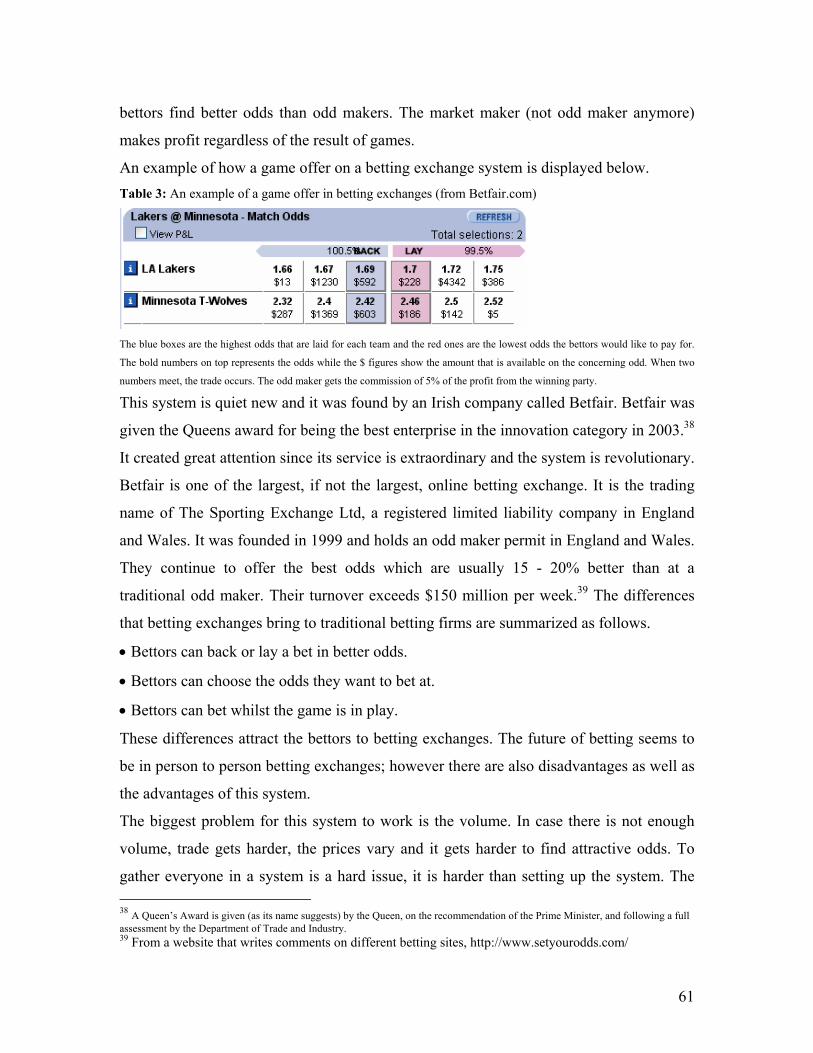
61

bettors find better odds than odd makers. The market maker (not odd maker anymore)

makes profit regardless of the result of games.

An example of how a game offer on a betting exchange system is displayed below. Table 3: An example of a game offer in betting exchanges (from Betfair.com)

The blue boxes are the highest odds that are laid for each team and the red ones are the lowest odds the bettors would like to pay for.

The bold numbers on top represents the odds while the $ figures show the amount that is available on the concerning odd. When two

numbers meet, the trade occurs. The odd maker gets the commission of 5% of the profit from the winning party.

This system is quiet new and it was found by an Irish company called Betfair. Betfair was

given the Queens award for being the best enterprise in the innovation category in 2003.38

It created great attention since its service is extraordinary and the system is revolutionary.

Betfair is one of the largest, if not the largest, online betting exchange. It is the trading

name of The Sporting Exchange Ltd, a registered limited liability company in England

and Wales. It was founded in 1999 and holds an odd maker permit in England and Wales.

They continue to offer the best odds which are usually 15 - 20% better than at a

traditional odd maker. Their turnover exceeds $150 million per week.39 The differences

that betting exchanges bring to traditional betting firms are summarized as follows.

• Bettors can back or lay a bet in better odds.

• Bettors can choose the odds they want to bet at.

• Bettors can bet whilst the game is in play.

These differences attract the bettors to betting exchanges. The future of betting seems to

be in person to person betting exchanges; however there are also disadvantages as well as

the advantages of this system.

The biggest problem for this system to work is the volume. In case there is not enough

volume, trade gets harder, the prices vary and it gets harder to find attractive odds. To

gather everyone in a system is a hard issue, it is harder than setting up the system. The 38 A Queen’s Award is given (as its name suggests) by the Queen, on the recommendation of the Prime Minister, and following a full assessment by the Department of Trade and Industry. 39 From a website that writes comments on different betting sites, http://www.setyourodds.com/

62

start of a company using this system is almost the hardest part of the job. Heavy

advertising, special offers, introducing a new system to people and the threat from the

major companies in the business are very tough obstacles to overcome. But once it is

settled, it is a profitable business; without any hedging skills, the odd maker makes

money whoever wins the game. All odd maker has to do is to offer the games and gather

the volume for it.

Another problem with low volume is that it can create speculative movements in the

market. A large volume customer can simply speculate the prices and make profits: buy

all high odds, lay on lower odds and this way an arbitrage opportunity occurs regardless

of the game result. Low volume is always dangerous as it is also the case in stock

markets.

After witnessing the development of betting exchanges, it is hard to predict where betting

markets are leading to. This research ends with an idea for the future of the betting in the

following.

A think tank: What is next for betting?

The Internet is very important for betting exchanges. All trades occur online. The firms

earn on the bets with a commission. What comes to mind is, can the bettors get rid of this

commission? Just like in the illegal music sharing over the internet, could the bettors

exchange odds between each other without a commission or just paying the wire cost? A

software program, just like the file sharing programs over the internet could do this

easily. A firm with such a product can actually have a great income by just putting

advertisement to the program. Instead of commission, advertisements could secure the

firm a good income and the users would enjoy a fair competition. Kazaa, the file sharing

program, serves customers the opportunity to share music for free and is making money

only from advertisements. A sharing software program could work the same way for

betting. This is actually possible on theory but there is no such development yet. In my

opinion big credit card firms, such as VISA or Mastercard might like to get involved to a

development which they already have familiar system and would increase the use of their

cards. Moreover they would enjoy a big income once they overcome the volume and the

security problem. Yet this kind of development would be very dangerous for the

traditional gambling firms and drop their income just like the music companies’ profit

63

decreased after Kazaa’s software. It would at least be as risky as Kazaa’s development,

lawsuits and licenses would all be the problem. Yet since it would use internet, the

international law would rule and the company would probably be found as innocent as

Kazaa, which has won the lawsuits from the music producers and continue to provide

sharing between internet users.40 Such a development would create almost a frictionless

market and be one step closer to being an efficient market.

Even this idea could be another topic for a research that aims to find an ideal market.

Betting markets offer ideas like this to scientists. It is researcher’s work to get inspired

and implement it to other markets.

By this part it was aimed to make a brainstorming of what could be the next thing for

betting markets. It might sound unrealistic, yet if achieved; it would be one of the closest

markets to being frictionless.

Conclusion

This study aimed to research betting markets from a behavioral finance point of view.

The effort is spent to learn from an alternative market that promises data and research

opportunities. It has been a long literature survey starting with traditional finance, went

on with efficient markets hypothesis, behavioral finance, psychology and finally betting.

Furthermore betting markets are analyzed from a behavioral finance point of view.

This study provides a detailed guide for new researches in the field. In this way, the aim

of researching betting markets is fulfilled. The industry figures, market structure, key

issues are studied. Thus, there are several results of this study to underline at the end.

A major finding that should be underlined is the similarity of the investor and bettor

traits. This research showed that the findings in behavioral finance about investor

behaviors are consistent with bettor behaviors. As a conclusion, investors can observe

biases and traits that drive bettors and learn from an alternative type of decision making.

These observations can help investors to make risk involved decisions more rationally. It

provides a broader view for investors and hints about their biases.

40 This is personal view of the researcher and should not be considered for any reliance on any future development

64

An important result is that the first expectation of this study is confirmed: behavioral

finance helps explaining the betting markets. Behavioral Finance especially helps

analyzing bettor behaviors. Moreover, as explained in detail above, findings in this

different structure have interesting clues for the behavioral finance. Scientists have

important results in data from these markets.

The empirical work on the replication of Brown and Sauer (1993) showed consistent

result with more recent data. The results provided a fundamental value of approximately

80% which is a high level for a market. It states that the comparison of the abilities of

each team highly explains the point spreads.

A major problem that was observed during the research is the applicability to financial

markets. Betting markets serve a good data base for the financial researches, and there are

some serious theories tested on these markets. Many of these researches are published in

famous journals. Some of them included significant results that were never achieved in

financial markets. However, this is only one side of the story: The importance of these

researches seems like it does not satisfy the scientists. There are very few researches

which quote these test results in betting markets. It seems that these researches performed

successful tests and achieved some results, yet their impact is not very impressive. The

first reason that comes to mind is that it is hard to convince people that findings in betting

markets could reflect a significant result for a much more complicated market like the

stock exchange. The controlled laboratory environment is accused to be too simplistic

and the controlled issues are actual variables in financial markets. My view on this issue

is that people do not see the betting markets as an alternative market. They do not believe

that the results of these researches can be adjusted to financial researches. Even the

researches that found significant results in this field end their papers with a conclusion

that states their findings can not be easily transferred to other markets. What found is

accused to be characteristic to betting markets. Moreover, there is a high conservatism on

testing financial theories in markets like sports betting which is seen as a symbol of a

market that is set to take the money and the bettor apart.

In my opinion, the problem is that the researches are too focused on testing the

hypotheses and running the empirical effort in betting markets while the applicability to

finance was left out. My suggestion for further researches would be to overcome this

65

adjustability problem. The findings, no matter how important they are, have to be

adjusted to the financial markets. Therefore, in this sense, the researches in betting

markets have been disappointing.

Moreover, risk management skills of odd makers were seen in search of the market

structure. The theories on the how the odds are set provided interesting hedging skills to

analyze these markets. These theories can give hints for risk managers in their field.

Betting markets have a complex structure. By this study, this structure and how things

work in this market were explained in detail. The findings provide guidance to further

betting researches. It was an interesting and exciting field to track the footprints of

rationality and finance rules. It has been a great journey on an alternative market to

search clues of more complicated ones; financial markets. In this sense, this paper

achieved to conduct a “consilience” on an alternative field, sports betting markets.

66

References

Ali, M., “Probability and utility estimates for racetrack bettors.” J. Political Economy 82

803-815. (1977).

Asch, P., B.G. Malkiel and R.E. Quandt. “Racetrack betting and informed behavior.” J.

Financial Economics 10 187-194. (1982).

Arrow, K. J.. “Information and economic behavior.”, 1982, Collected Papers of K. J.

Arrow, volume 4, Basil Blackwell, Oxford, (1984).

Avery, C., Chevalier, J., , “Herding Over the Career”, Economics Letters 63, 327-33.

(1999)

Bachelier L., "Theorie de la Speculation" Annales de l'Ecole Normale Superieure,

(1900).

Balestra, M., “Internet Gambling Report”, River City Group, (2004).

Barberis, N., Thaler, R., "A Survey of Behavioral Finance. " NBER Working Paper

W9222. 2002

Barrett, C., “5 Types of gamblers identified”, From the article by Mark Curnutte,

Cincinnati Enquirer, 19 Dec, (1996)

Bird, R., McCrae, M. “Tests of the efficiency of racetrack betting using bookmaker

odds.” Management Science 33, 1552-1562. (1987).

Black, F., Scholes, M. "The pricing of options and corporate liabilities," Journal of

Political Economy 81, 637-654, (1973)

Black, F., “Noise”, Journal of Finance, 41, 529-43 (1986).

De Bondt, W. F. M., Thaler, R.H., “Does the stock market overreact ?” Journal of

Finance 40, 793-805, (1985).

Brown, W. and Sauer R.D., , “Fundamentals or Noise? Evidence from the professional

basketball betting market”, Journal of Finance, Vol. 48, No. 4, 1193-1209 1993

Burns, B., “The hothand in basketball: Fallacy or adaptive thinking?” Department of

Psychology, Michigan State University, 2004

Camerer, C., “Does the market believe in hot-hand?”, The American Economic Review,

79-5, (1989)

67

Camerer, C. F., Hogarth R., “The effects of Financial Incentives in Experiments: A

review and Capital Labor Production Framework”, Journal of Risk and Uncertainty 19,

7-42, (1999).

Chapple, C., Nofziger, S.,. “Bingo!: Hints of Deviance in the Accounts of Sociability

and Profit of Bingo Players”. Deviant Behavior 21(6): 489-517, (2000).

Cowles, A., "Can Stockmarket Forecasters Forecast?" In: Econometrica Vol. 1: 309-324,

(1933).

Cox, J.C., Ingersoll J., and Ross S., "A theory of the term structure of interest rates,"

Econometrica 53, 385-407(1985)

De Long J. B., Shleifer A., Summers, L. H. and Waldmann, R. J., 1990, "Noise trader

risk in nancial markets", Journal of Political Economy, 98(4), 703-738.

Duffie, J. D. and Huang, C.,"Implementing Arrow-Debreu equilibria by continuous

trading of a few long-lived securities." Econometrica, 53, 1337-1356. 32 (1985).

Edwards, W., “Conservatism in Human Information Processing”, in B. Kleinmutz, ed.,

Formal Representation of human Judgment, New York: John Wiley and Sons, (1986).

Evans, R., Gauthier, D.K., and Forsyth, C.J., “Dogfighting: Symbolic expression and

validation of masculinity.” Sex Roles, 39(11/12), 825-838. (1998)

Falk, R., & Konold, C. “Making sense of randomness implicit encoding as a basis for

judgment.” Psychological Review, 104, 301-318, (1997)

Fama, E. F., “Efficient Capital Markets: Review of Theory and Empirical Work”, Journal

of Finance 25, 383-417, (1970)

Feeney, R., King, S.P.,”Sequential Pari-mutuel Games”, Department of Economics, The

University of Melbourne, (2003)

Fischoff B., Slovic P.,Lichtenstein, S., "Knowing with Certainty: The Appropriateness

of Extreme Confidence." Journal of Experimental Psychology: Human Perception and

Performance 3(4), 552-564 (1997)

Fisher, I, “The Nature of Capital and Income”, Pickering &Chatto Press, (1906)

Fisher, I, “The Rate of Interest”, Pickering & Chatto Press, (1907),

Fisher, I, “Theory of Interest”, Pickering & Chatto Press, (1930).

Friedman, M., "Essays in Positive Economics," University of Chicago Press, Chicago,

(1953)

68

Gandar, J., Zuber, R., O’Brien, R., Russo, B., “Testing Rationality in the Point Spread

Market”, The Journal of Finance, 43 (September), 995-1008. (1988)

Gigerenzer, G., & Todd, P. M.. “Fast and frugal heuristics: The adaptive tool box.” In

G. Gigerenzer, P. Todd, & the ABC Research Group (Eds.), Simple heuristics that make

us smart (pp. 3-34). New York: Oxford University Press. (1999)

Gilden, D. L., & Wilson, S. G. “Streaks in skilled performance.” Psychonomic Bulletin

&Review, 2, 260-265. (1995).

Gilovich, T., Vallone, R., & Tversky, A. “The hot hand in basketball: On the

misperception of random sequences.” Cognitive Psychology, 17, 295-314. (1985).

Golec, J., Tamarkin, M., “The Degree of Inefficiency in the Football Betting Market”

Journal of Financial Economics vol. 30 pp. 311-323, (1991)

Golec, J., M. Tamarkin, “Bettors Love Skewness, Not Risk, at the Horse Track” Journal

of Political Economy 106, 205-225. (1998)

Gray, P K., Gray, S, “The Efficiency of Australian Football Betting Markets,”

Australian Journal of Management, Vol. 20, No. 2, 167-196. (1995)

Gray, P. K., Gray, S. F. “Testing Market Efficiency: Evidence from the NFL Sports

Betting Market,” Journal of Finance, 52, 4, 1725-1737. (1997)

Gross, L., , “The art of selling intangibles: How to make your million by investing other

people’s money”, Prentice Hall, (1985).

Grossman, S., and J. Stiglitz "On the impossibility of informationally efficient markets,"

American Economic Review 70, pp. 393-408, (1980).

Hantover, J. P., “The Boy Scouts and the validation of masculinity.” Sociological Issues,

34, 184-195. (1978).

Harris, L., Gurel, E., Price and Volume Effects Associated with Changes in the S&P

500, Journal of Finance, 41, 815--829. (1986).

Harrison, J.M. and D. Kreps, “Martingales and arbitrage in multiperiod securities

markets”, Journal of Economic Theory 20, 381-408 (1979).

Hart, O., "On the Optimality of Equilibrium when the Market Structure is Incomplete,"

Journal of Economic Theory, Vol. 11, No. 3, pp. 418-443, (1975).

69

Hayek, F.A., “The Use of knowledge in society”, American Economic Review, 35, 519-

530, (1945)

Hausch, D.B.; Ziemba, W.T.; and Rubinstein, M. “Efficiency of the market for

racetrack betting.” Management Science 27:1435-52, (1981).

Heath, C., Tversky, A., “Preference and beliefs: ambiguity and competence in choice

under uncertainty”, Journal of Risk and Uncertainty, 4:5-28, (1991)

Hicks, J., “Value and Capital: An inquiry into some fundamental principles of economic

theory”, Clarendon Press, Oxford, (1939)

Hicks, J, "Some Aspects of Commodity Markets", Manchester Guardian, (1923)

Houthakker, H., “Can Speculators forecast prices?”, The Review of Economics and

Statistics, Harvard University Press, (1957)

Houthakker, H., “Systematic and Random Elements in Price Movements”, American

Economic Review, (1961)

Houthakker, H., "Normal Backwardation", Value Capital and Growth, (1968)

Houthakker, H., Magee, S.P., "Income and Price Elasticities in World Trade", The

Review of Economics and Statistics, (1969)

Hurlbert, J. S., Bankston, W.B., “Cultural Distinctiveness in the Face of Structural

Transformation: The "New" Old South.” In D. R. Hurt (Ed.), Social Change in the Rural

South: 1945-1995. Baton Rouge: Louisiana State University Press, (1998).

Jay, R., “A Profile of the online gambler”, report for gambling firms, 2003

Kaldor, “Welfare Propositions in Economics", Economic Journal, (1939)

Kendall, M. G. "The Analysis of Economic Time Series," Journal of the Royal Statistical

Society (Series A), XCVI, 11-25, (1953).

Keim, D. B., “Size-Related Anomalies and Stock Return Seasonality”, Journal of

Financial Economics, pp 13-32, (1983).

Keynes, J., “A Treatise on money”, Prometheus Books, (1930)

Koessler, F. , Broihanne, M. H. & Ziegelmeyer, A., , “The Favorite-Longshot Bias in

Sequential Parimutuel Betting with Non-Expected Utility Players”, Theory and Decision,

, 54(3), 231-248, (2003)

Levitt, S.D., “How Do Markets Function? An Empirical Analysis of Gambling on the

National Football League” NBER Working Paper No. 9422, (2002).

70

Lintner, J.,"Security Prices, Risk, and Maximal Gains from Diversification” Journal of

Finance 20, (1965), 587-615.

Loomes G., Sugden, R. “Regret theory: An alternative theory of rational choice under

uncertainty.” The Economic Journal, 92:805--824, (1982).

Lucas, Robert, “Asset prices in an exchange economy”, Econometrica 46, 1429-1445.,

1978

Malkiel, B., Asch P.,"Market efficiency in racetrack betting" Journal of Business, (1984)

Mandelbrot, B. B., “When can price be arbitraged efficiently? A limit to the validity of

the random walk and martingale models”, Review of Economics and Statistics. 53, 225-

236, (1971).

Markowitz, H., “The utility of Wealth”, Journal of Political Economics, (1952)

Marschak, J., “Money and the Theory of Assets”, Econometrica, (1938)

Merton, R., "An intertemporal capital asset pricing model," Econometrica 41, 867-888.

(1973)

Merton, Robert C. “Theory of rational option pricing.” Bell Journal of Economics and

Management Science, 4:141--183, (1973).

Miyoshi, H. “Is the "hot-hands" phenomenon a misperception of random events?”

Japanese Psychological Research. 42, 128-133. (2000).

Milgrom, P., Stokey, N., "Information, Trade and Common Knowledge," Journal of

Economic Theory 26: 17--27., (1982).

Moggridge, D., “Collected Writings of John Maynard Keynes, Vol. 7 - The General

Theory” ,(1973)

Modigliani, F., Miller, M. H. "The Cost of Capital, Corporation Finance, and the

Theory of Investment," American Economic Review, 48, pp. 261-297, (1958).

Modigliani, F. and M. Miller, "Corporate Income Taxes and the Cost of Capital: A

Correction," American Economic Review, 53, pp. 433-443. (1963).

National Gambling Impact Study Commission, “Report of Gambling Impact and

Behavior Study”, University of Chicago, (1999).

Neumann, J. V., Morgenstern, O., “Theory of Games and Economic Behavior”,

Princeton University Press, (1944).

71

Niederhoffer, V., “The Analysis of World Events and Stock Prices”, Journal of Business,

Volume 44, Issue 2, 193-219, (1971)

O'Neil, J. M., “Gender role conflict and strain in men's lives.” In K. S. N. B. Levy (Ed.),

Men in Transition: Theory and Therapy, New York: Plenum Press. (1982).

Oster, E., “Powerball lottery”, Harvard College Research Program Award winner final

project, (2002)

Ottowani, M., Sørensen, P.N., “Late informed betting and Favorite-Long shot Bias”,

Journal of Economic Literature, 2003

Radner, R.,“Competitive equilibrium under uncertainty” Econometrica 36, 31-58,(1968)

Radner, R.,"Existence of Equilibrium of Plans, Prices, and Price Expectations in a

Sequence of Markets," Econometrica, 40, 289-303, (1972)

Roll., R., “A critique of the asset pricing theory's tests” Journal of Financial Economics,

4:129--176, (1977)

Roll, Richard W., “Ambiguity when Performance is Measured by the Securities Market

Line," Journal of Finance, Volume 33 (4), pp. 1051-1069.(1978)

Ross, S.A., “The Arbitrage Theory of Capital Asset Pricing.”, Journal of Economic

Theory 13, 341-360, (1976).

Ross, S. A., “Essentials of Corporate Finance”, McGraw-Hill, 2001

Rubinstein, A., “Economics and Language”, Cambridge University Press, (2000)

Samuelson, P. A., “A Proof That Properly Anticipated Prices Fluctuate Randomly”,

Industrial Management Review 6(Spring), 41-50, (1965).

Sharpe, W., “Capital asset prices: A theory of market equilibrium under conditions of

risk”, Journal of Finance 19, (1964), 425-443

Shefrin. “Beyond Greed and Fear: Understanding Behavioral Finance and the

Psychology of Investing”. Oxford University Press, New York, (2002).

Shiller, R.J. "The volatility of long-term interest rates and expectations models of term

structure," Journal of Political Economy 87, 1190-1219, (1979).

Shiller, R., “Human Behavior and The Efficiency of the Financial System”, Handbook of

Macroeconomics, Taylor & Woodward, (1997).

Schnytzer, A. and Y. Shilony, “Inside Information in a Betting Market," The

Economic Journal, 105, 963-971. (1995)

72

Slovic, P. & Lichtenstein S., “Comparison of Bayesian and regression approaches to

the study of information processing in judgment”, Organizational Behavior and Human

Resources, 6, 649-744, (1971).

Stevenson, R. A., Bear, R.M., “Commodity Futures: Trends or Random Walks?”,

Journal of Finance, Volume 25, Issue 1 65-81. (Mar., 1970)

Strumpf, K., “Illegal Sports Betting”, Journal of Political Economy, (2003)

Summers, L., “Does the Stockmarket rationally reflect fundamental values?”, Journal of

Finance, 41-3, 591-602, (1986).

Telser, L., "Futures Trading and the Storage of Cotton and Wheat", Journal of Political

Economics, (1958)

Telser, L., “Why There Are Organized Futures Markets”, Journal of Law and

Economics, (1981)

Thaler, R. H. and W. T. Ziemba. “Anomalies: Parimutuel betting markets: Racetracks

and lotteries.” Journal of Economic Perspectives, 2(2):161--174, (1988).

Tobin, J., "Money, Capital and Other Stores of Value", American Economic Review,

(1961)

Trueman, B., “A Theory of Noise Trading in Securities Markets”, Journal of Finance,

Volume 43, Issue 1 83-95, (Mar., 1988).

Tversky, A., Kahneman, D., "Judgement under uncertainty: Heuristics and biases."

Science, Vol. 125, pp. 1124-31, (1974).

Tversky A., Kahneman, D. "Prospect theory: An analysis of decision under risk,"

Econometrica 47:263—291, (1979)

Tversky, A., Kahneman, D., "Variants of uncertainty.", Cognition, 11, 143-157, (1981)

U.S. Congressional Report, “Internet Gambling: An Overview of the Issues”, US

General Accounting Office, (2002).

Volberg, R., “Gambling and Problem gambling in Louisiana”, Gemini Research Ltd.,

(1999)

Waiman P., Hraba, M., "Age and Gambling Behavior: A Declining and Shifting

Pattern of Participation," Eadington and Cornelius, eds., pp. 56-59, (1997).

Walker, M. B., “The Psychology of Gambling”. Oxford: Pergamon Press., 1992

73

Weinstein, N. "Unrealistic Optimism About Future Life Events," Journal of Personality

and Psychology, 39(5): 806—820, (1980).

Weintraub, R. E., “On Speculative Prices and Random Walks A Denial”, Journal of

Finance, Volume 18, Issue 1 59-66. (1963)

Wildman, R., II. “Gambling: An Attempt at an Integration”. Edmonton, Alberta, Wynne

Resources (1997).

Williams, J., “The theory of Investment Value”, Fraser Publishing, (1938)

Wilson, E.O., “Consilience.” The Unity of Knowledge, Abacus, London, (1998).

Woodland, L., Woodland, B., “Market Efficiency and Profitable Wagering in the

National Hockey League: Can Bettors Score on Longshots?” Southern Economic Journal

67(4), 983-995. (2001)

Working, H., , “A Random difference series for use in the analysis of time series”,

Journal of the American Statistical Association 29,11-24., 1934

74

Appendix

75

Appendix A: Betting Glossary

Action: A live bet or bets.

Arbitrage: Betting the same event at separate sports books in order to lock in a profit by

taking advantage of different betting lines.

Bankroll: Total capital available for betting sports.

Board: A presentation of all the games and events available for betting in a sports book.

(If wagers are being taken on a game, the game is "on the board," otherwise it is "off the

board.")

Bookmaker (or bookie): A person who accepts bets.

Buyback: The money that comes in on the underdog after a favorite is bet heavily

enough to move the line.

Chalk: A favorite, usually a heavy favorite.

Chalk eaters: Bettors who like to bet big favorites (often a derogatory term).

Circled game: A game in which the sports book has reduced its betting limits, usually

due to weather or the uncertain status of injured players.

Cover: Winning against the point spread. (A 10-point underdog that loses 20-14 has

covered, or "covered the spread.")

Exposure: The degree of risk that a sports book will lose money on a given game, result,

or proposition. (If a book is "highly exposed" on the Cubs in World Series futures betting,

it will lose a lot of money to bettors if the Cubs win the World Series.)

Fade (Lay): To take the opposite side of another bettor's wager, or to accept that bet

yourself.

76

Favorite: A team (or player) that, according to the odds, is the stronger or strongest in a

given matchup, or is regarded as such by the betting public, or is expected to win.

First-half betting: Wagers that involve the outcome of the first half of a game only.

Freeroll: A bet one can win or “push”, but not lose.

Futures: A type of wager involving the outcome of a season or how a particular team or

player will perform over the course of a season.

Halftime betting: Wagers, based on betting lines posted at halftime, which involve the

outcome of the second half of a game only.

Handicap: Point spread for soccer games.

Handle: The amount of money in wagers accepted. ("The handle was down this year on

the Super Bowl.")

Hedge: To make a bet that takes the opposite side of your original position, usually to

reduce risk or lock in some profit.

House: The casino, sports book, or bookmaker.

Lay: See fade.

Layoff: A type of wager made by one bookmaker with another, often larger bookmaker

in order to balance action or reduce risk.

Limit: The maximum wager accepted by a sports book.

Line: The point spread or odds on a game or event.

Lock: A bet that cannot lose

Long shot: The team that has a low chance of winning on a game.

77

Matchup proposition: A betting option that pits two players against one another in a

contest or event, often used in golf and auto racing wagering.

Middle: A situation in which one bets both sides in a game and wins both bets, due to

favorable line moves. (Example: Bet a football favorite at minus 2 ½, then bet the

underdog at plus 3 ½ at another book or later in the week. If the favorite wins by exactly

3 points, both bets win.)

Money line: The odds on a team winning a game outright, regardless of the point spread.

Offshore: Designation for the organized sports betting industry outside of the United

States.

Out: A place to get bets down, whether it's a Nevada sports book, offshore book or

illegal bookmaker. ("It's good to have a lot of outs.")

Over/under: See "totals."

Overlay: A situation in which the odds are favorable to the sharp bettor.

Parlay: A bet in which two or more events must happen in order to win; if any one of

them does not happen, the wager loses.

Player: A sports bettor.

Pleaser: A specialized form of a parlay that improves the point spread (for the book) but

pays off at improved odds.

Point spread: The number of points added to or subtracted from a team's actual score for

betting purposes.

Price: See "line."

Proposition (or prop): An unusual or offbeat betting opportunity.

78

Public: Average, unsophisticated or casual bettors as a whole; or, used to describe money

bet by the public ("a lot of public money came in on the Cowboys"); see "square."

Puck line: In hockey, a betting structure that dictates the favorite must win by a set

number of goals, and/or adds a set number of goals to the underdog's actual score.

Push: A bet in which the money wagered is refunded; a tie.

Rotation: The official list of all the games on the betting board, presented in a specific

order.

Round robin: A specialized form of a parlay that uses every combination of a set of

teams in a wager. For example, there would be six two-team parlays within a four-team

round robin.

Rundown: A reading of all the games and betting lines on a particular day.

Runner: See "beard."

Scalp: A form of a middle in which one bets both sides in a game, taking advantage of

line movements to secure a profit.

Sharp: Savvy, highly informed; or, used to describe the money bet by sharp players ("a

lot of sharp money came in on the Eagles").

Side: A variation of a middle in which you win one bet and push the other; also, a

particular team in a matchup. ("Which side do you like?")

Sports book: The part of the casino that accepts bets on athletic contests or a sports

betting firm.

Square: An unsophisticated or casual bettor, the opposite of a wise guy; see "public."

Steam: One-sided action.

79

Straight: A single bet, usually laying 11 to win 10.

Teaser: A specialized form of a parlay that improves the point spread (for the bettor) but

pays off at reduced odds.

Totals: A type of wager that involves whether a score or result will go over or under a

posted number.

Tout: A person who sells his predictions to bettors (often derogatory).

Underdog: A team (or player) that, according to the odds, is the weaker or among the

weakest in a given matchup, or is regarded as such by the betting public, or is expected to

lose.

Vigorish (or vig): The commission charged by the bookmaker.

Wise guy: A sharp, successful, established professional sports bettor.

Wood: The price of a heavy favorite.

80

Appendix B Model Summary for 1999-2000

Model R R Square Adjusted R

Square Std. Error of the Estimate

1 ,874(a) ,763 ,757 3,02490 Model Summary for 2000-2001

Model R R Square Adjusted R

Square Std. Error of the Estimate

1 ,887(a) ,787 ,781 2,77669 Model Summary for 2001-2002

Model R R Square Adjusted R

Square Std. Error of the Estimate

1 ,872(a) ,760 ,754 2,94093 Model Summary for 2002-2003

Model R R Square Adjusted R

Square Std. Error of the Estimate

1 ,898(a) ,806 ,801 2,72359 a Predictors: (Constant), WASHINGT, LAKERS, CLIPPERS, NEWORLEA, PHOENIX, PHILADEL, DALLAS, MILWAUKE, MINNESOT, TORONTO, BOSTON, SEATTLE, PORTLAND, ATLANTA, GOLDENST, INDIANA, MEMPHIS, NEWJERSE, HOUSTON, DETROIT, ORLANDO, DENVER, UTAH, CHICAGO, SACRAMEN, NEWYORK, CLEVELAN, SANANTON, MIAM

81