Embed Size (px)
Citation preview
Benchmarking FORTRAN 90 Array Operations
Author - Tom Mead ([email protected])
Project Supervisor - Tim Hopkins ([email protected])
Autumn 2003 - Spring 2004
Abstract Fortran is still used in scientific programming because of it’s efficiency and the optimal code the variety of compilers on the market can produce. We test these ideas by benchmarking different types of array routines. We describe the importance of benchmarking and its uses in determining the most suitable solutions. We offer conclusions about which ones to use and in which situations and why they generate the performance they do. 1. Introduction
If you ask Fortran programmers or search the web for ”why use Fortran” then one answer comes up regularly. It goes something like “Fortran 90 is good at manipulating arrays”. There is just reason for this, a lot of the changes between Fortran 77 and Fortran 90 are array manipulation orientated. Fortran is also quite a low level programming language so it is expected to be fast and if coded well, efficient.
Fortran is fundamentally a scientific and
engineering based language, the name itself is an acronym for “formula transition”. The first Fortran compliers were built in the 1950’s and represented a huge leap forward in the use of computers. As its popularity grew, the number of platforms it was developed for also grew. Compilers for different operating systems and hardware were developed by organisations catering for their own needs. This caused problems due to the lack of portability so in 1966 ANSI defined Fortran IV as the standard edition. It is now more commonly referred to as Fortran 66. In 1977, Fortran 77 was defined. It added relatively few features but the new standard reflected the sort of companies using it as an integral part of their systems. In the
nineties it was again redefined as Fortran 90 which is the version I will be investigating.
Aside from recent years, use of the processor, especially in engineering applications has been strictly monitored to ensure maximum efficiency. Programmers learnt the best ways to perform operations so that the processor would be used in the most resourceful way. Vector supercomputers such as the Cray–1S could take advantage of their machines hardware. Programmers were encouraged to develop their code to maximise the benefits of this. The following code (Fortran 77 – Cray CFT Compiler) would be optimised by the compiler[3]:
DO 20 I=1, N K=I+1 A(K) = B(I)
20 CONTINUE However, with CPU speeds increasing
beyond the limit of most programs needs, it has become hard, if not impossible to see the benefits of apply optimised methods. Compiler developers have noticed styles programmers use and have adapted and optimised code to become as fast as possible while still implementing the programmers intention.
Constant redefinition over the years and a myriad of different areas of development by the companies driving Fortran has lead to an extensive set of code, supplementary to the core set being produced. Fortran’s long history has meant that redefinition of code must be backwards compatible. Code fundamental to many applications must still be catered for while allowing new features to be introduced. To avoid this, new and different implementations of tools have been created.
This work looks at a commonly used
subset of operations, matrix and vector related subroutines. Matrices are extremely common in engineering applications as well as being fundamental to programming languages and mathematics. There are two general types of routines, intrinsic, and Basic Linear Algebra Subprograms (BLAS). We will also write
equivalent code in standard Fortran code to mimic the routines. For example, in the following code SDOT, the BLAS routine and the following loop produce the same results: REAL (arraySize) :: oneV, twoV REAL dummyVar !BLAS dummyVar=SDOT(arraySize,oneV,1,twoV,1) !Loop dummyVar= 0 DO i = 1, arraySize dummyVar=dummyVar+(oneV(i)*twoV(i) END DO On some of the operations, BLAS or intrinsic routines will not be applied as they are unsuitable or not equivalent. For example the intrinsic maximum and minimum functions cannot be compared with their BLAS counterparts. This is because BLAS uses absolute values to find the extremities while the intrinsic functions do not. Comparing the different methods for speed would be unfair as the BLAS is handicapped by having to strip each value of its sign.
The intention of this project is to develop a program to time and output these operations on a number of different platforms. We would like this program to use the widest range of operating systems, hardware types and compilers. Due to this restriction any programs written must be portable and reliable to ensure when they are run, they will work and they will return accurate results. Once a comprehensive set of data is produced, conclusions relating to the best routines to be used will be reached. 2. Benchmarking
“A series of tests performed in order to
gage and set the performance of computer components and subsystems, benchmarking is performed in order to compare results of one computer with other known computer standards.[4]” This is a very general quote describing the uses and implications of benchmarking. Benchmarking any sort of system requires us to define a measurement unit that we can associate with any system and compare with another. Once this comparison has been made this measurement allows us to evaluate which system works best.
Trying to find a definition for ‘best’ is very hard regarding benchmarking. For
example, how would you measure the best computer? A 3 GHz CPU with 16Mb of RAM is just as useless as a 100MHz CPU with 1Gb of RAM. With operations though, it is slightly more obvious. Speed of processing is the ultimate requirement. Operations must meet up to other criteria as well though. Results must be as accurate as required, i.e. to the correct amount of decimal places. Functionality must be provided for, it would be impractical to use five functions in preparation for an operation when a similar operation can do it all at once.
Benchmarking is made easier by always
comparing with similar systems that have applications which are as alike as possible. This means that it is likely that you will be able to compare the two systems using the same measurement and the functionality offered by them will be similar. Sometimes an obvious unit of measurement leads to inaccurate conclusions. For instance Gigahertz is the obvious unit for measuring processor speed. Still many lower clocked processors beat their higher counterparts. This is because the processors with inferior clock ratings are sometimes better at real work, i.e. not theoretical. They sometimes produce higher floating point operations per seconds compared to their rivals. It is important to be mindful of this when designing a benchmarking suite since simply measuring the time it takes to perform an operation does not give a complete picture of what is going on. For example, I will be using random data following an equal distribution whereas in a real application data will follow trends. Fortunately this is not usually relevant in matrix operations. Obscure implications of test data are very unlikely, but it but it does illustrate how benchmarking follows a standard path and routine, when the real world is definitely not standard.
Even though benchmarking is prone to give a blurred view of a system it does provide a view and that is what is important. Without benchmarking systems it would be impossible to know what state of development you are currently at. Without knowing your current state it would be impossible to realise what areas are weak and what areas need improving. By benchmarking several systems with different implementations bottlenecks can be found. Once a bottleneck in a system is found it can be compared with similar systems to see which parts are different and which are most likely to be causing problems.
The gaming software and hardware
industry has become geared towards
benchmarking and optimisation. Similarly to an optimised compiler hardware can be tweaked to maximum performance. Nevertheless the problems associated with optimised compiler usage are also similar to hardware optimisation. Reliability is never guaranteed with optimised products without comprehensive testing. Regular testing harnesses may not pick up on optimised compiler code irregularities just like an over clocked CPU may overheat as it is not capable of running at the increased clock rate.
Benchmarking is necessary in the
development of the array operations. If it is seen that they are lacking in performance and/or functionality then there is little point in keeping them around. Of course backwards compatibility restricts this culling technique. New versions and implementations of Fortran mean that it is important that old routines are profiled to see what should be included. Re-implementing or optimising a routine may be an obvious step forward once it is known what problems or bottlenecks exist.
3. BLAS routines
The BLAS routines were developed to perform vector and matrix operations[5]. They are building blocks that are used to make more complicated operations[6]. When BLAS were first introduced they were envisaged as model routines. It was intended that hardware manufactures would produce their own highly tuned versions of the library. This would mean that BLAS functionality would be identical on any system but hardware could take advantage of of its own implementations to achieve maximum performance. LAPACK is another group of Fortran routines. It uses BLAS routines to solve linear algebra and associated equations. BLAS is used in LAPACK in this case as it offers tested, high quality and well supported routines. The routines offer more functionality than regular vector and matrix operations.
For instance SGEMM, the matrix
multiplication routine makes use of thirteen parameters[7]:
SGEMM(transa , transb , l, n, m, alpha , a, lda , b, ldb , beta , c, ldc) The standard routine, MATMUL is much simpler to use and only requires two parameters[8]:
MATMUL([MATRIX_A=]mat_a,[MATRIX_B=]mat_b) The parameter issue derives from the Fortran 77 implementation of SGEMM where restrictions on how arrays would be manipulated were needed. The BLAS implementation is computationally more general. In Fortran 90 these restrictions were lifted, simplifying calls. The BLAS routine is much more customisable and can be tailored to suit the specific task. If we take: REAL(size) :: matrix1, matrix2,matrix3 An inexperienced developer, for instance, might code the following: TRANSPOSE(matrix1) TRANSPOSE(matrix2) matrix3 = MATMUL(matrix1, matrix2)
While this code will generate the intended results, the following will do all three operations on the fly: SGEMM(‘T’ , ‘T’ , ‘N’ , size, size , 1, matrix1 , size , matrix2 , size , 0, matrix3 , size)
As a result of performing the routine in one go, less operations should be needed to produce the results. Instead of having to copy new results for both matrices into memory and then perform a matrix operation on them, all operations can now be performed as and when they are needed. It is important to remember that the functions are not completely equivalent. The first example actually manipulates the source arrays into a transposed position. The second example just outputs the result as if the arrays were transposed from the beginning. This is fine if the array parameters are no longer needed, especially in their original state.
The BLAS routine contains a lot of
functionality that is redundant in most matrix multiplication operations. However, it’s features means more complicated multiplication can be simplified and as the parameters can be given in character form, they are dynamic and can be set and altered during runtime. The large amount of redundant functionality although adding to its viability for general use should mean that the BLAS matrix multiplication will be considerably slower. It is still likely to be used in engineering and scientific applications as it is more versatile a tool. Its customisable nature
means that developers need not write as much code for problems that occur regularly. 4. Test suite
The test suite must be able to test a range
of different types of operation. All operations are grouped together in subroutines so they are all completed at similar times and when the system has similar processing loads. Allocating all similar operations into a subroutine means that it simplifies matters if the user wishes to run only a subset of operations. If they should want to do so they can select which type of tests by changing a vector with elements corresponding to whether the operations should be run. At runtime the program can loop through all possible operation groups and determine which should be run. An array of operation timings can be passed back to the main program from any subroutines. This array can then be processed and outputted when needed. We will be testing using REAL data types. Other versions of BLAS routines are available that implement double precision, complex etc are available but this benchmark serves as a base model or prototype for other, very similar routines.
The test suite is capable of producing
vectors and matrices full of random data for the various operations to use. The type of array (vector or matrix) depends on the sort of operation. SGEMV requires a vector and a matrix while SDOT requires two vectors. This decision is made just before they are required. The arrays are given size dynamically using the ALLOCATE operation. This means that array space can be continually increased until it is large enough to time an operation accurately.
All tests are ideally carried out a multiple
of times. When the computer and processor load are at its least, the performance is at its best. This means that for x number of runs, only one timing will be used. This result will be the smallest. As the best or smallest timing is copied its relative MegaFLOPS rate is copied as well. There is no point copying the best MegaFLOPS rate, it could correspond to a different timing and be inaccurate because of the array size used. The smallest will have the least noise. Noise being time taken by the computer processing jobs unrelated to the benchmark. As some computers are busiest during the day or other peak hours it is best to run the benchmarking test when other jobs are not running. This is usually in the night when the least amount of users and therefore
applications, are running. This means that the benchmarking software should not require user interaction.
To avoid user input the program must be
define its own parameters as it runs. That is, it must manipulate its variables so the results are worth recording. There is no point of a benchmarking program saying it completed all the operations in 0.001 seconds as it is inaccurate and does not tell us anything about the operations. General default variables must be initialised to low values if they are to be run on lower specification computers. The first instance of the benchmarking test must be one that every platform will perform quickly on. Once a operation is established as too easy, more difficult (increased size) parameters can be set. This progression is called burning-in[9]. To prevent burning in going on forever in the event of a runtime error for instance, an upper bound is required. After a set number of increases in difficulty the test suite will stop even if optimal results have not been recorded. Without this the program could grow so that it would crash the computer it is running on before it would finish the operation. This fact is worrying and technically difficult to avoid in all cases. The program must try its best to get large enough to become useful without becoming too large for the host system to handle. If the benchmarking software manages to stop itself growing too big it may mean that there is no useful data retrieved for that test. However, if it avoids a crash it could mean that it is possible to run the next test successfully.
Array operations are much like any other
system, they have input , processing and output. It is important to realise that all array operations are fundamentally the same. Then it becomes easy to provide systematic means to test them all. To ensure a fair test is provided all array operations of a similar type must be tested in fundamentally identical environments. All functions which requires an array of random data and an empty array must get that and not just the first one to be tested. It is not satisfactory to use the results from another array operation as a set of random data. The data should come from the same random data generation algorithm for every time the operation is tested.
Result timings are also be represented in
MegaFLOPS. MegaFLOPS are an independent unit for measuring data and can be compared without having to take many other things into account. Obviously the machine it is running on is still a factor but as it is a ratio to how
much work is being done a valid reading can always be compared with another.
Data retrieved from the benchmarking
tests will only be useful if it can be interpreted easily. Initially I thought a text based tabular format would be good with an indication of which result is the best. This is a good method as it allows the user to quickly locate the fastest operation. Tables are good for displaying data as they allow a easy way for a user to cross reference information in their heads. Eventually I chose this to be a good way of displaying results quickly to the user as the benchmarking software is running. After each subroutine has completed timing the relevant operation a table of results is displayed on screen. This involves:
• final array size • operation title • method subtitles • method times • method MegaFLOPS (if available) • fastest method indicator Information about the size of array, results
from the most recent operation and meta data regarding timings being correct, too small or too large are constantly being displayed. This informs the user of the state of the system. As operation timing is completed the final results are outputted. This is done to a comma separated variable (CSV) file[10]. This was chosen because it is a relatively simple format to write to but it still gives users the option to open in a database or spreadsheet application. For comparing results at the end, graphs are preferable to evaluating tabular numbers so a spreadsheet is the best solution. XML is a viable more powerful but it seems like overkill in this situation. XML would require a considerably more complex output procedure. There are tools that will convert CSV available should XML be required, in fact most spreadsheet packages will be able to do this.
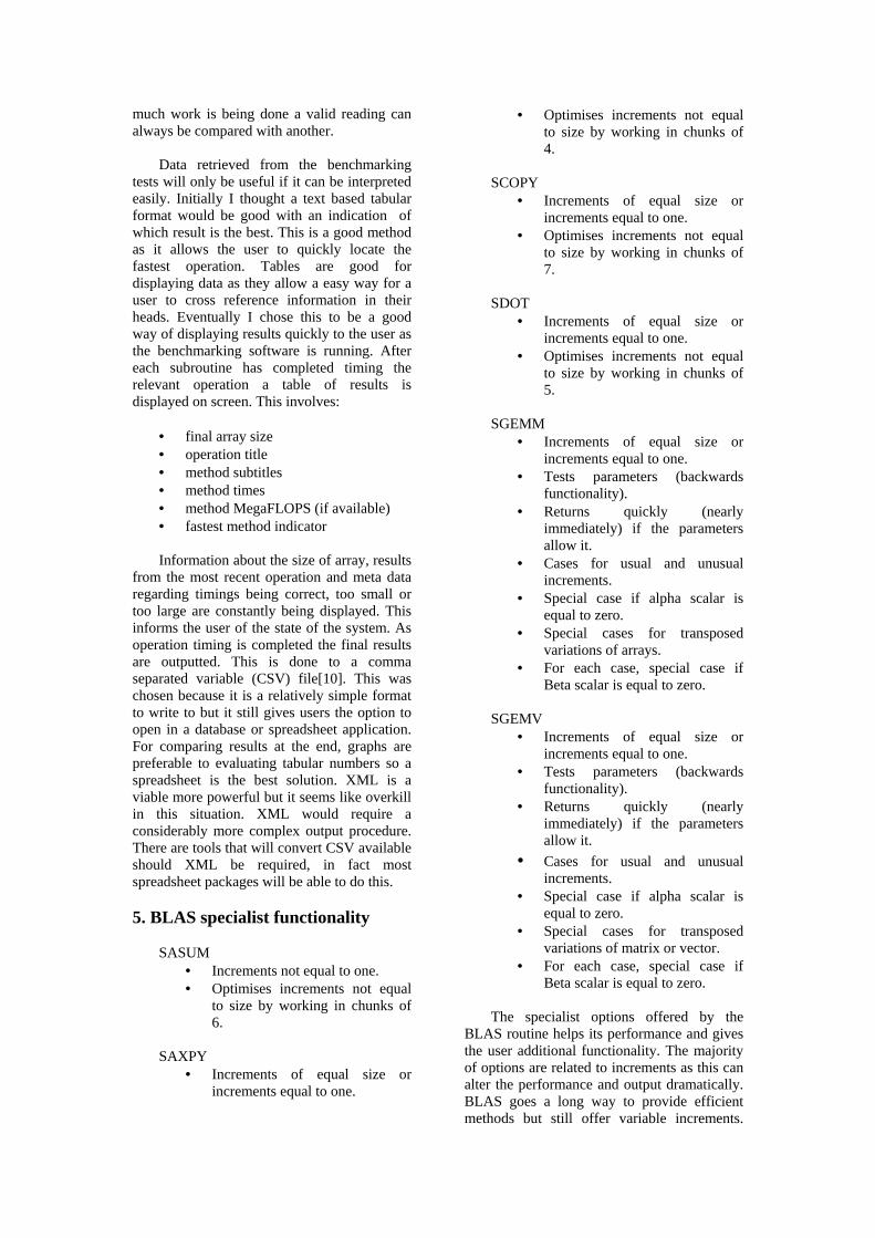
5. BLAS specialist functionality
SASUM
• Increments not equal to one. • Optimises increments not equal
to size by working in chunks of 6.
SAXPY
• Increments of equal size or increments equal to one.
• Optimises increments not equal to size by working in chunks of 4.
SCOPY
• Increments of equal size or increments equal to one.
• Optimises increments not equal to size by working in chunks of 7.
SDOT
• Increments of equal size or increments equal to one.
• Optimises increments not equal to size by working in chunks of 5.
SGEMM
• Increments of equal size or increments equal to one.
• Tests parameters (backwards functionality).
• Returns quickly (nearly immediately) if the parameters allow it.
• Cases for usual and unusual increments.
• Special case if alpha scalar is equal to zero.
• Special cases for transposed variations of arrays.
• For each case, special case if Beta scalar is equal to zero.
SGEMV
• Increments of equal size or increments equal to one.
• Tests parameters (backwards functionality).
• Returns quickly (nearly immediately) if the parameters allow it.
• Cases for usual and unusual increments.
• Special case if alpha scalar is equal to zero.
• Special cases for transposed variations of matrix or vector.
• For each case, special case if Beta scalar is equal to zero.
The specialist options offered by the
BLAS routine helps its performance and gives the user additional functionality. The majority of options are related to increments as this can alter the performance and output dramatically. BLAS goes a long way to provide efficient methods but still offer variable increments.
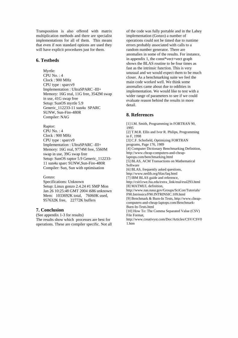
Transposition is also offered with matrix multiplication methods and there are specialist implementations for all of them. This means that even if non standard options are used they will have explicit procedures just for them. 6. Testbeds
Myrtle: CPU No. : 4 Clock : 900 MHz CPU type : sparcv9 Implementation : UltraSPARC -III+ Memory: 16G real, 11G free, 3542M swap in use, 41G swap free Setup: SunOS myrtle 5.9 Generic_112233-11 sun4u SPARC SUNW, Sun-Fire-480R Compiler: NAG Raptor: CPU No. : 4 Clock : 900 MHz CPU type : sparcv9 Implementation : UltraSPARC -III+ Memory: 16G real, 9774M free, 5560M swap in use, 39G swap free Setup: SunOS raptor 5.9 Generic_112233-11 sun4u sparc SUNW,Sun-Fire-480R Compiler: Sun, Sun with optimisation Gonzo: Specifications: Unknown Setup: Linux gonzo 2.4.24 #1 SMP Mon Jan 26 10:25:48 GMT 2004 i686 unknown Mem: 1033692K total, 76060K used, 957632K free, 22772K buffers
7. Conclusion (See appendix 1-3 for results) The results show which processes are best for operations. These are compiler specific. Not all
of the code was fully portable and in the Lahey implementation (Gonzo) a number of operations could not be timed due to runtime errors probably associated with calls to a random number generator. There are anomalies in some of the results. For instance, in appendix 1, the const*vect+vect graph shows the BLAS routine to be four times as fast as the intrinsic function. This is very unusual and we would expect them to be much closer. As a benchmarking suite we feel the main code worked well. We think some anomalies came about due to oddities in implementation. We would like to test with a wider range of parameters to see if we could evaluate reason behind the results in more detail.
8. References [1] I.M. Smith, Programming in FORTRAN 90, 1995 [2] T.M.R. Ellis and Ivor R. Philips, Programming in F, 1998 [3] C.F. Schofield, Optimizing FORTRAN programs, Page 176, 1989 [4] Computer Dictionary Benchmarking Definition, http://www.cheap-computers-and-cheap-laptops.com/benchmarking.html [5] BLAS, ACM Transactions on Mathematical Software [6] BLAS, frequently asked questions, http://www.netlib.org/blas/faq.html [7] IBM BLAS guide and reference, http://csit1cwe.fsu.edu/extra_link/essl/essl293.html [8] MATMUL definition, http://www.nas.nasa.gov/Groups/SciCon/Tutorials/F90.Intrinsics/F90.INTRINSIC.109.html [9] Benchmark & Burn-In Tests, http://www.cheap-computers-and-cheap-laptops.com/Benchmark-Burn-In-Tests.html [10] How To: The Comma Separated Value (CSV) File Format, http://www.creativyst.com/Doc/Articles/CSV/CSV01.htm

Appendix 1 Raptor – Sun compiler results
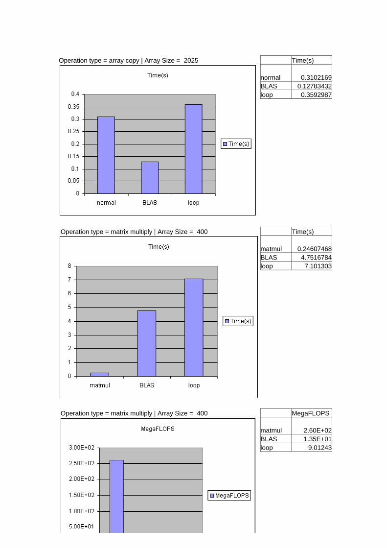
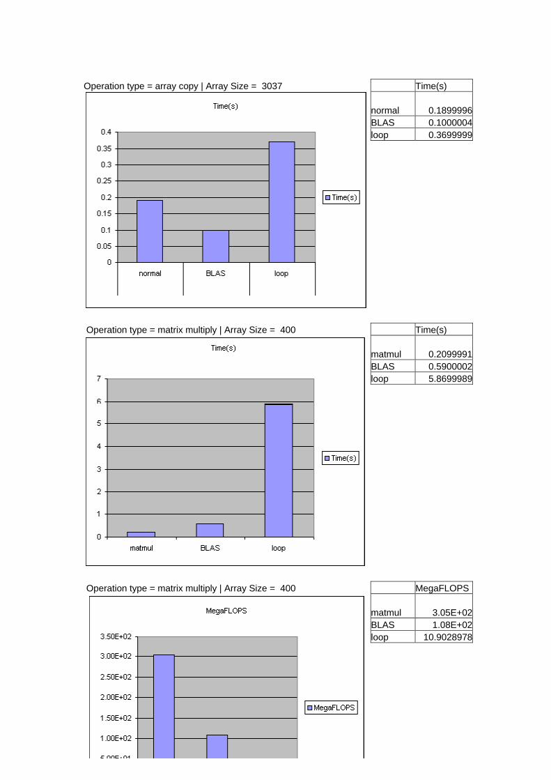
Operation type = array copy | Array Size = 2025 Time(s) normal 0.3102169 BLAS 0.12783432 loop 0.3592987
Operation type = matrix multiply | Array Size = 400 Time(s) matmul 0.24607468 BLAS 4.7516784 loop 7.101303
Operation type = matrix multiply | Array Size = 400 MegaFLOPS matmul 2.60E+02 BLAS 1.35E+01 loop 9.01243
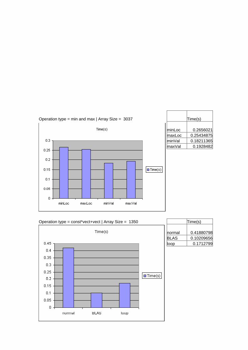
Operation type = min and max | Array Size = 3037 Time(s) minLoc 0.2656021 maxLoc 0.25434875 minVal 0.18211365 maxVal 0.1928482
Operation type = const*vect+vect | Array Size = 1350 Time(s) normal 0.41880798 BLAS 0.10209656 loop 0.1712799
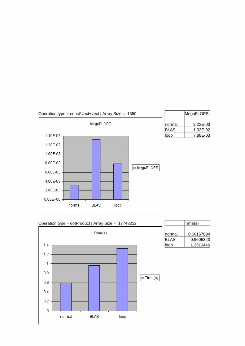
Operation type = const*vect+vect | Array Size = 1350 MegaFLOPS normal 3.22E-03 BLAS 1.32E-02 loop 7.88E-03
Operation type = dotProduct | Array Size = 17748212 Time(s) normal 0.60167694 BLAS 0.9606323 loop 1.3313446
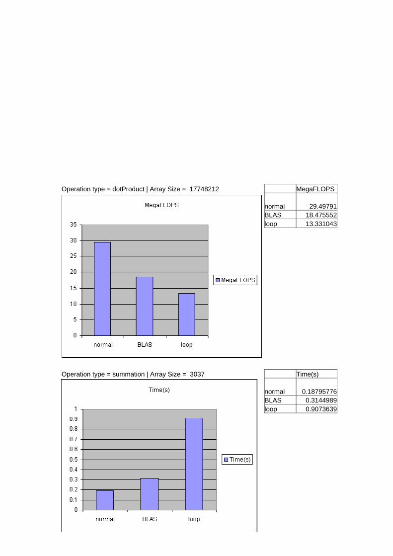
Operation type = dotProduct | Array Size = 17748212 MegaFLOPS normal 29.49791 BLAS 18.475552 loop 13.331043
Operation type = summation | Array Size = 3037 Time(s) normal 0.18795776 BLAS 0.3144989 loop 0.9073639
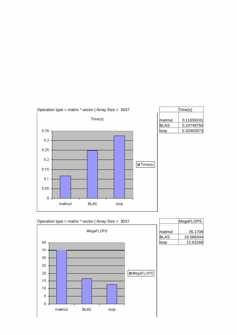
Operation type = matrix * vector | Array Size = 3037 Time(s) matmul 0.11659241 BLAS 0.24749756 loop 0.32463073
Operation type = matrix * vector | Array Size = 3037 MegaFLOPS matmul 35.1706 BLAS 16.568344 loop 12.63166

Appendix 2 Myrtle – NAG compiler results
Operation type = array copy | Array Size = 3037 Time(s) normal 0.1899996 BLAS 0.1000004 loop 0.3699999
Operation type = matrix multiply | Array Size = 400 Time(s) matmul 0.2099991 BLAS 0.5900002 loop 5.8699989
Operation type = matrix multiply | Array Size = 400 MegaFLOPS matmul 3.05E+02 BLAS 1.08E+02 loop 10.9028978
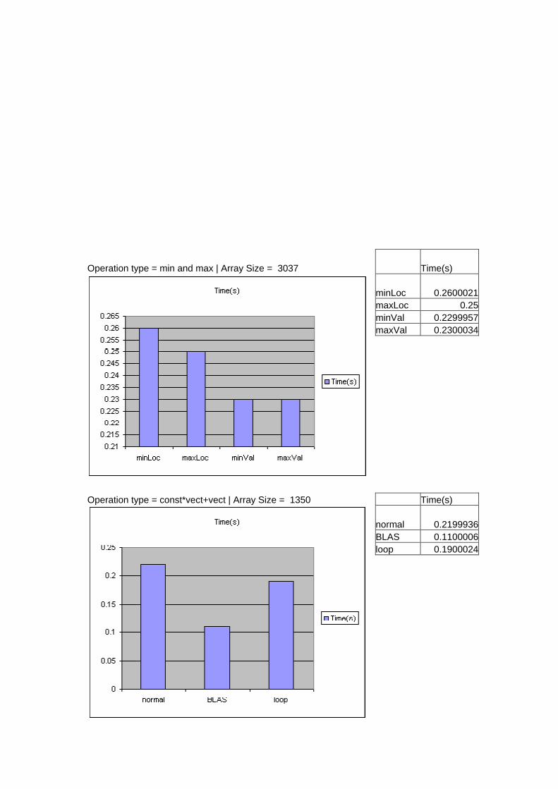
Operation type = min and max | Array Size = 3037 Time(s) minLoc 0.2600021 maxLoc 0.25 minVal 0.2299957 maxVal 0.2300034
Operation type = const*vect+vect | Array Size = 1350 Time(s) normal 0.2199936 BLAS 0.1100006 loop 0.1900024
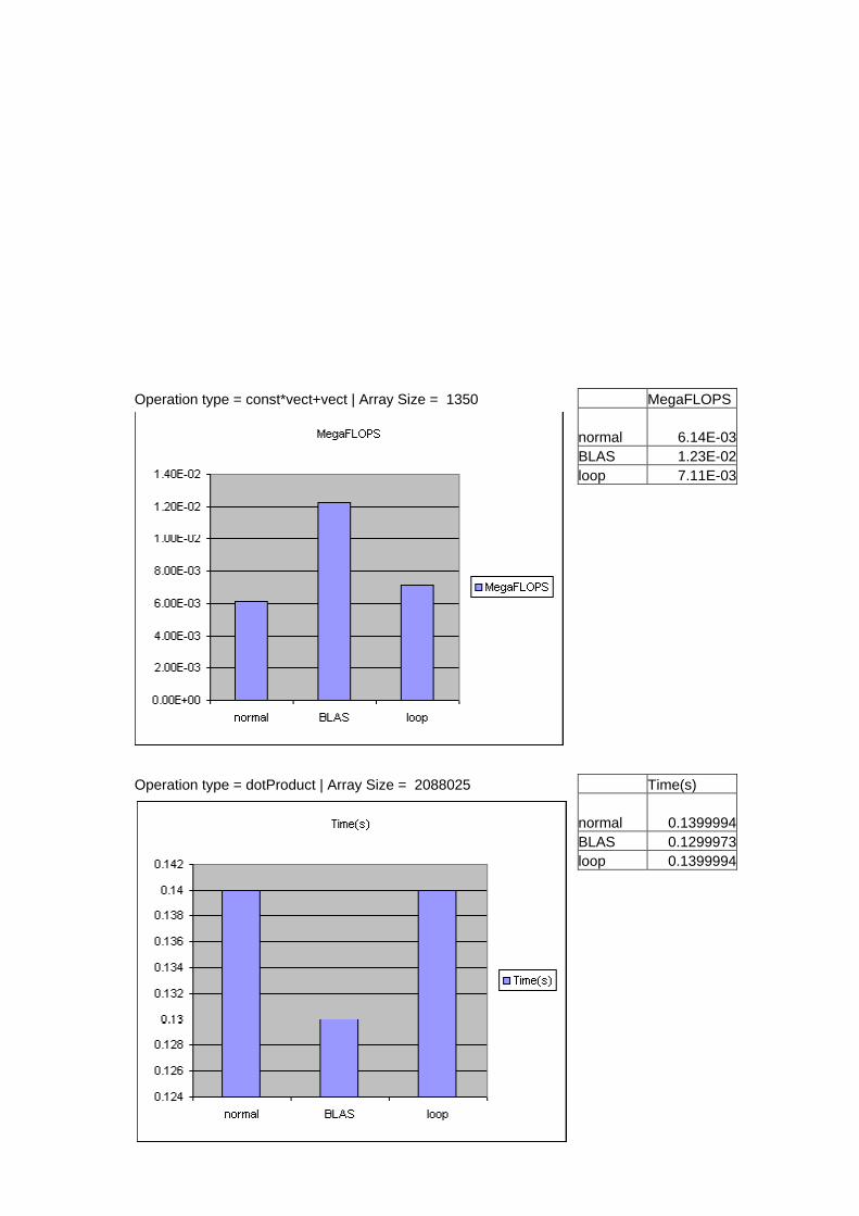
Operation type = const*vect+vect | Array Size = 1350 MegaFLOPS normal 6.14E-03 BLAS 1.23E-02 loop 7.11E-03
Operation type = dotProduct | Array Size = 2088025 Time(s) normal 0.1399994 BLAS 0.1299973 loop 0.1399994
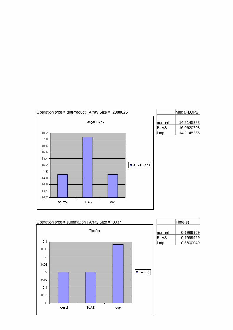
Operation type = dotProduct | Array Size = 2088025 MegaFLOPS normal 14.9145288 BLAS 16.0620708 loop 14.9145288
Operation type = summation | Array Size = 3037 Time(s) normal 0.1999969 BLAS 0.1999969 loop 0.3800049
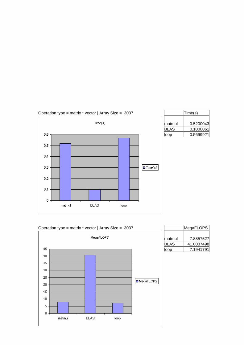
Operation type = matrix * vector | Array Size = 3037 Time(s) matmul 0.5200043 BLAS 0.1000061 loop 0.5699921
Operation type = matrix * vector | Array Size = 3037 MegaFLOPS matmul 7.8857527 BLAS 41.0037498 loop 7.1941791

Appendix 3 Gonzo – LAHEY compiler results
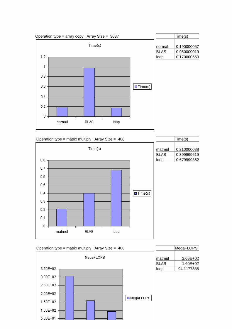
Operation type = array copy | Array Size = 3037 Time(s) normal 0.190000057 BLAS 0.980000019 loop 0.170000553
Operation type = matrix multiply | Array Size = 400 Time(s) matmul 0.210000038 BLAS 0.399999619 loop 0.679999352
Operation type = matrix multiply | Array Size = 400 MegaFLOPS matmul 3.05E+02 BLAS 1.60E+02 loop 94.1177368
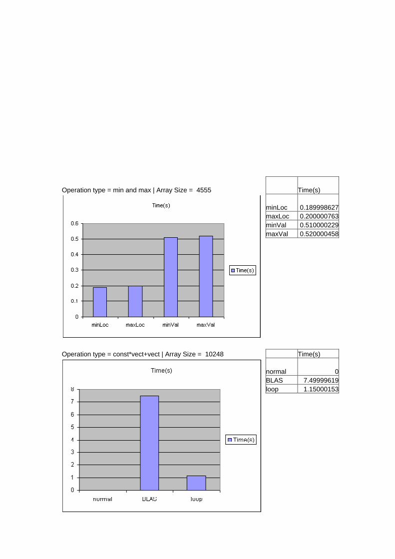
Operation type = min and max | Array Size = 4555 Time(s) minLoc 0.189998627 maxLoc 0.200000763 minVal 0.510000229 maxVal 0.520000458
Operation type = const*vect+vect | Array Size = 10248 Time(s) normal 0 BLAS 7.49999619 loop 1.15000153
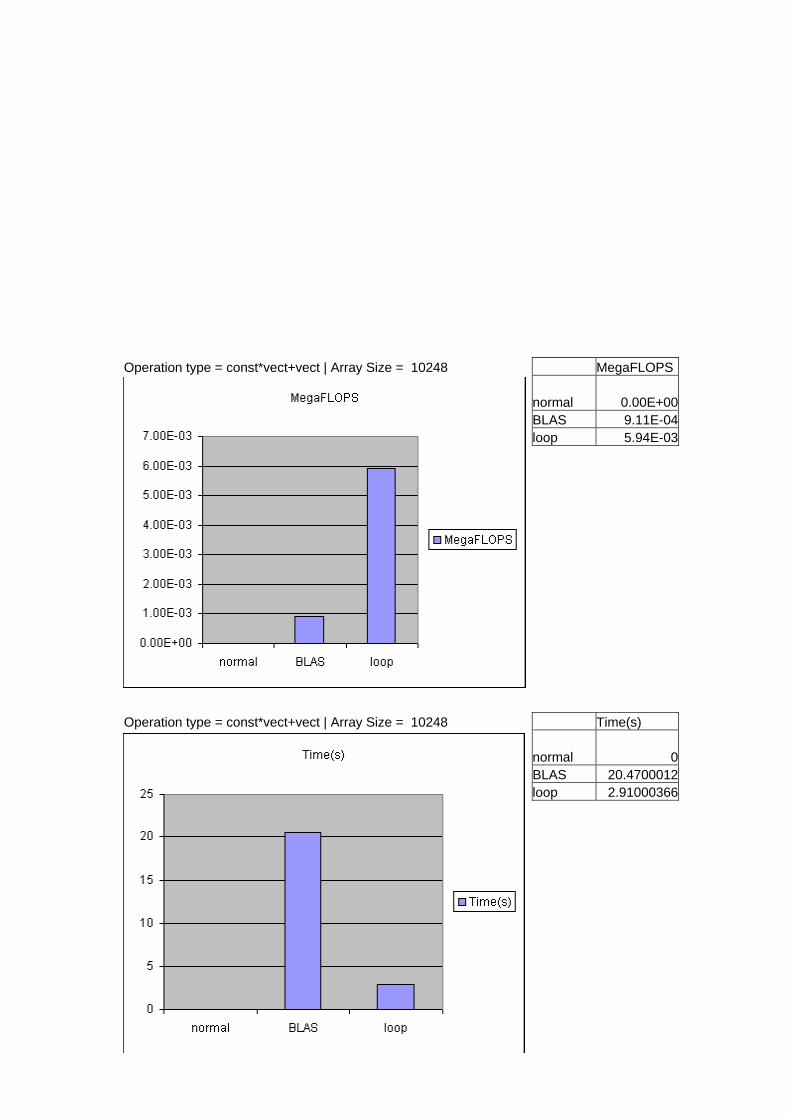
Operation type = const*vect+vect | Array Size = 10248 MegaFLOPS normal 0.00E+00 BLAS 9.11E-04 loop 5.94E-03
Operation type = const*vect+vect | Array Size = 10248 Time(s) normal 0 BLAS 20.4700012 loop 2.91000366
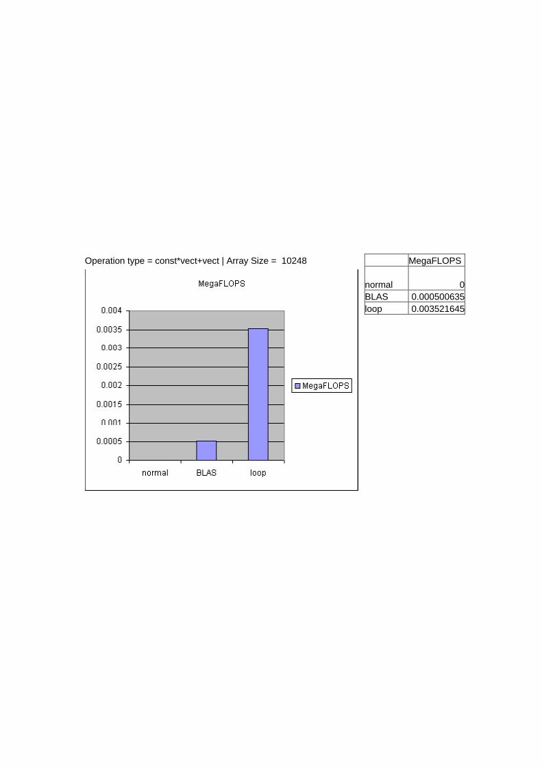
Operation type = const*vect+vect | Array Size = 10248 MegaFLOPS normal 0 BLAS 0.000500635 loop 0.003521645