Bene ts of collocating vertical-axis and horizontal-axis wind turbines in large wind … Library/Our People/Profiles... · Beneﬁts of collocating vertical-axis and horizontal-axis

RESEARCH ARTICLE

Benefits of collocating vertical-axis and horizontal-axiswind turbines in large wind farmsShengbai Xie1, Cristina L. Archer1, Niranjan Ghaisas2 and Charles Meneveau3

1 College of Earth, Ocean, and Environment, University of Delaware, USA2 Center for Turbulence Research, Stanford University, USA3 Department of Mechanical Engineering, Johns Hopkins University, USA

ABSTRACT

In this study, we address the benefits of a vertically staggered (VS) wind farm, in which vertical-axis and horizontal-axiswind turbines are collocated in a large wind farm. The case study consists of 20 small vertical-axis turbines added aroundeach large horizontal-axis turbine. Large-eddy simulation is used to compare power extraction and flow properties of theVS wind farm versus a traditional wind farm with only large turbines. The VS wind farm produces up to 32% more powerthan the traditional one, and the power extracted by the large turbines alone is increased by 10%, caused by faster wakerecovery from enhanced turbulence due to the presence of the small turbines. A theoretical analysis based on a top-down model is performed and compared with the large-eddy simulation. The analysis suggests a nonlinear increase of totalpower extraction with increase of the loading of smaller turbines, with weak sensitivity to various parameters, such as size,and type aspect ratio, and thrust coefficient of the vertical-axis turbines. We conclude that vertical staggering can be an ef-fective way to increase energy production in existing wind farms. Copyright © 2016 John Wiley & Sons, Ltd.

KEYWORDS

wind farm; HAWT; VAWT; large-eddy simulation

CorrespondenceCristina L. Archer, College of Ocean, Earth and Environment, University of Delaware, Newark, Delaware 19716, USA.E-mail: [email protected]/grant sponsor: National Science Foundation; contract/grant numbers: 1357649, IIA-1243482.

Received 9 July 2015; Revised 18 March 2016; Accepted 1 April 2016

1. INTRODUCTION

With the increasing demand for renewable energy globally, wind farms, especially offshore wind farms, have continued to in-crease in size. It is well known that the energy loss in a large wind farm can be due in large part to the interactions between windturbines and wind turbine wakes.1–6Wake losses can be reduced by using a staggered layout of the wind turbines in the horizontaldirections. A wind farm is called ‘horizontally staggered’ when wind turbines in consecutive rows are not aligned behind eachother along the wind direction. Wind direction effects have been systematically studied for the Horns Rev offshore wind farmby Porté-Agel et al.7 using large-eddy simulation (LES). They found that even small changes in wind direction can have strongimpacts on the total wind farm’s power output. Chamorro et al.8 used wind tunnel measurements of miniature turbine models tostudy turbulent properties of a horizontally staggered wind farm. They found that turbulence in the horizontally staggered windfarm resembles that in the wake of a single turbine, which is substantially different from that in an aligned configuration. More-over, the overall power output was improved by about 10% in the horizontally staggered farm. The variations in momentum, sca-lar and kinetic energy fluxes between aligned and horizontally staggered model wind farms have been revealed by theexperimental study of Markfort et al.9 From both LES and wind tunnel experiments of 30 miniature wind turbines, Wu andPorté-Agel10 found that the horizontally staggered layout leads to higher local wind speed, lower turbulence intensity and conse-quently higher turbine efficiency. Stevens et al.6 used LES to study the influence of the alignment of wind turbine rows inside alarge wind farm and found an increase in power generation up to 40% by an intermediate alignment configuration. The effects ofspacing and horizontal staggering of wind turbines in the Lillgrund wind farm (in Sweden) have been systematically studied using

WIND ENERGYWind Energ. (2016)

Published online in Wiley Online Library (wileyonlinelibrary.com). DOI: 10.1002/we.1990

Copyright © 2016 John Wiley & Sons, Ltd.

LES by Archer et al.,11 where they found that total power generation was increased by 13% in the horizontally staggered layoutand that the capacity factor was improved by 33% by combining both staggering and larger spacing.

Besides the horizontal staggering, the effects of staggering wind turbines in the vertical direction have also been studied in afew previous works. Chamorro et al.12 studied amodel wind farm consisting of miniature horizontal-axis wind turbines (HAWTs)of two sizes (i.e., two hub heights and rotor areas). Distinctive flow features were observed, which impacted power harvesting andturbulence loading. The effects of variable hub heights (with the same rotor area) of HAWTs were investigated experimentally byVested et al.,13 and 25% higher power was reported for the variable-height wind farm than for the traditional one.

In this study, out of the many possible vertical staggering types, a new approach is proposed, hereafter referred to simply asVS, which is particularly feasible for existing wind farms, in which neither the position nor the height of the existing HAWTscan be changed. Given a control wind farm comprising of traditional, large HAWTs, all with the same hub height, the spacebetween the large turbines is filled with much smaller, shorter and lower capacitywind turbines, e.g., vertical-axis wind turbines(VAWT). The smaller turbines are used to capture the lower, but (for the most part) undisturbed winds that blow below the rotortips of the large turbines. The smaller turbines can have vertical or horizontal axes of rotation, but the former are studied herebecause of their low cost and wide availability today in the low-capacity market.14 There has been considerable recent interestin VAWT wind farms.15 The major issue here is whether or not the presence of the layer of smaller turbines would adverselyaffect the energy harvested by the large HAWTS.

In this study, the VS wind farm is studied with advanced numerical simulations and with an analytical model and itsperformance is evaluated against its traditional counterpart, a HAWT farm in which no vertical staggering is used.

2. NUMERICAL SIMULATIONS

2.1. Methods and setup

Large-eddy simulation is used here to study the staggering of a wind farm in the vertical. LES is a numerical technique thatresolves the large-scale flow motions and includes the effects of small-scale eddies via sub-grid scale models.16 In this study,the LES model used is a pseudo-spectral version of the wind turbine and turbulence simulator developed at University of Del-aware.17 For solving the filtered Navier–Stokes equations, the Fourier series-based spectral method is used in the horizontaldirections with periodic boundary conditions, and the second-order finite difference method is used in the vertical direction.The 2/3 rule is implemented for elimination of the aliasing errors.18 A second-order Adams–Bashforth scheme is used for timeintegration, and the Lagrangian-averaged scale-dependent model is used for the subgrid-scale (SGS) modeling.19 The wind tur-bine aerodynamics are treated as body forces with the actuator-line model, where the lift and drag coefficients of each airfoilsection along each blade are determined from tabulated data according to upstream wind speed and local angle of attack.20

More details of wind turbine and turbulence simulator and its validations can be found in Xie and Archer17 and Xie et al.21

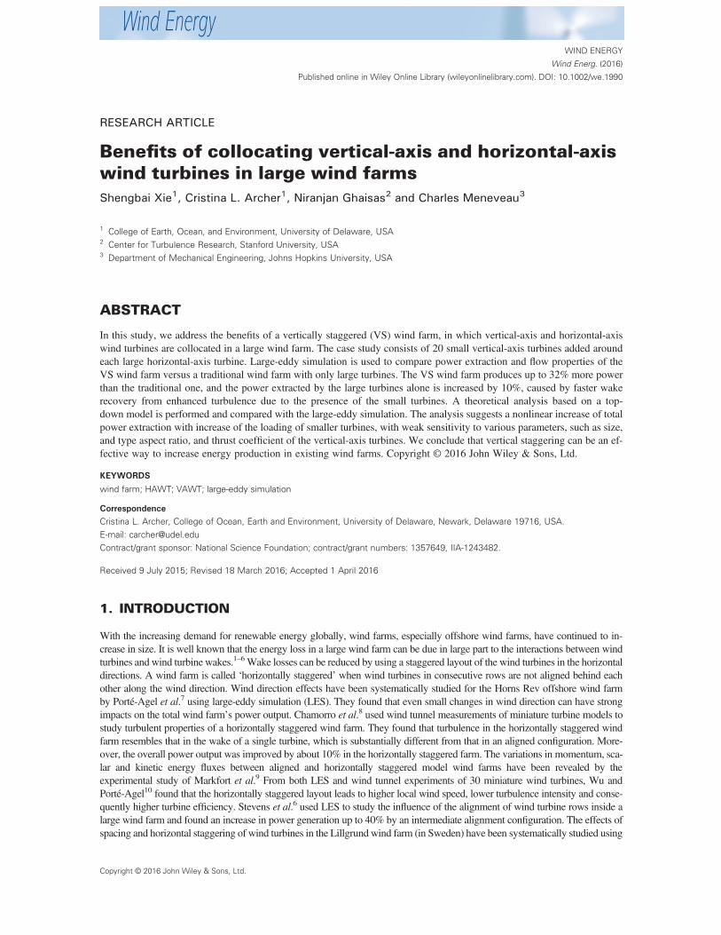
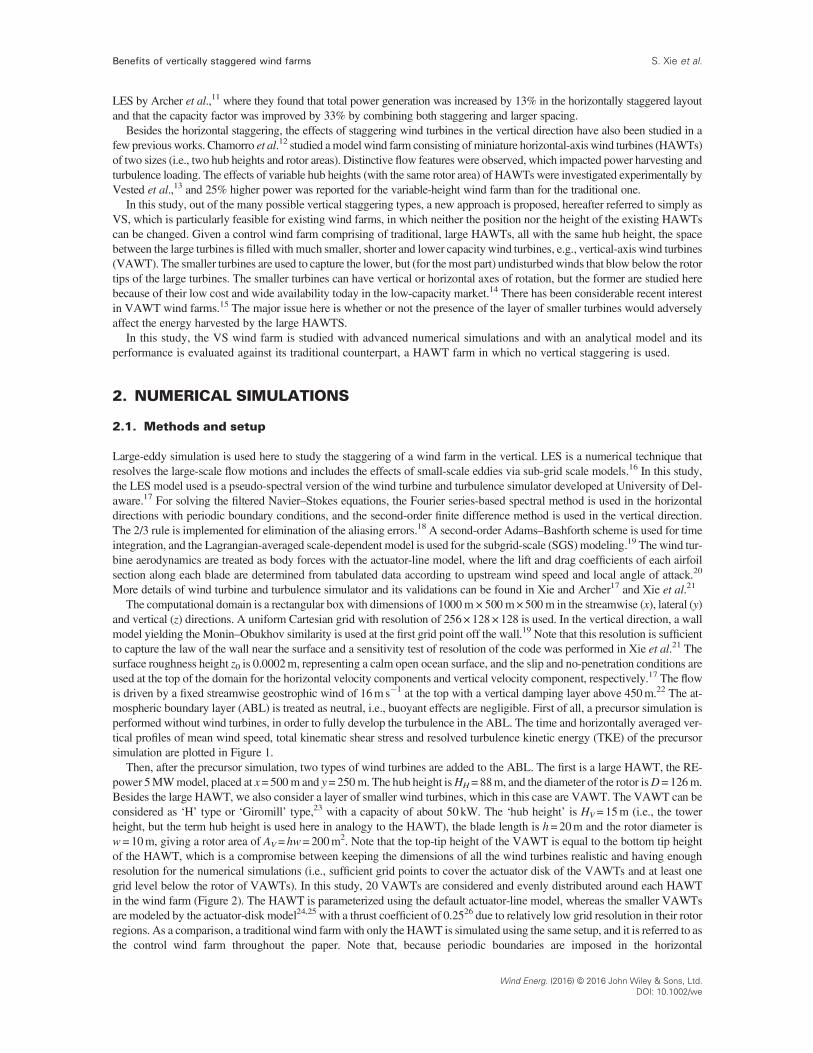
The computational domain is a rectangular box with dimensions of 1000m × 500 m× 500m in the streamwise (x), lateral (y)and vertical (z) directions. A uniform Cartesian grid with resolution of 256× 128× 128 is used. In the vertical direction, a wallmodel yielding the Monin–Obukhov similarity is used at the first grid point off the wall.19 Note that this resolution is sufficientto capture the law of the wall near the surface and a sensitivity test of resolution of the code was performed in Xie et al.21 Thesurface roughness height z0 is 0.0002m, representing a calm open ocean surface, and the slip and no-penetration conditions areused at the top of the domain for the horizontal velocity components and vertical velocity component, respectively.17 The flowis driven by a fixed streamwise geostrophic wind of 16m s!1 at the top with a vertical damping layer above 450m.22 The at-mospheric boundary layer (ABL) is treated as neutral, i.e., buoyant effects are negligible. First of all, a precursor simulation isperformed without wind turbines, in order to fully develop the turbulence in the ABL. The time and horizontally averaged ver-tical profiles of mean wind speed, total kinematic shear stress and resolved turbulence kinetic energy (TKE) of the precursorsimulation are plotted in Figure 1.

Then, after the precursor simulation, two types of wind turbines are added to the ABL. The first is a large HAWT, the RE-power 5MWmodel, placed at x=500m and y=250m. The hub height isHH=88m, and the diameter of the rotor isD=126m.Besides the large HAWT, we also consider a layer of smaller wind turbines, which in this case are VAWT. The VAWT can beconsidered as ‘H’ type or ‘Giromill’ type,23 with a capacity of about 50 kW. The ‘hub height’ is HV=15m (i.e., the towerheight, but the term hub height is used here in analogy to the HAWT), the blade length is h=20m and the rotor diameter isw=10m, giving a rotor area of AV= hw=200m2. Note that the top-tip height of the VAWT is equal to the bottom tip heightof the HAWT, which is a compromise between keeping the dimensions of all the wind turbines realistic and having enoughresolution for the numerical simulations (i.e., sufficient grid points to cover the actuator disk of the VAWTs and at least onegrid level below the rotor of VAWTs). In this study, 20 VAWTs are considered and evenly distributed around each HAWTin the wind farm (Figure 2). The HAWT is parameterized using the default actuator-line model, whereas the smaller VAWTsare modeled by the actuator-disk model24,25 with a thrust coefficient of 0.2526 due to relatively low grid resolution in their rotorregions. As a comparison, a traditional wind farmwith only the HAWT is simulated using the same setup, and it is referred to asthe control wind farm throughout the paper. Note that, because periodic boundaries are imposed in the horizontal

Benefits of vertically staggered wind farms S. Xie et al.

Wind Energ. (2016) © 2016 John Wiley & Sons, Ltd.DOI: 10.1002/we

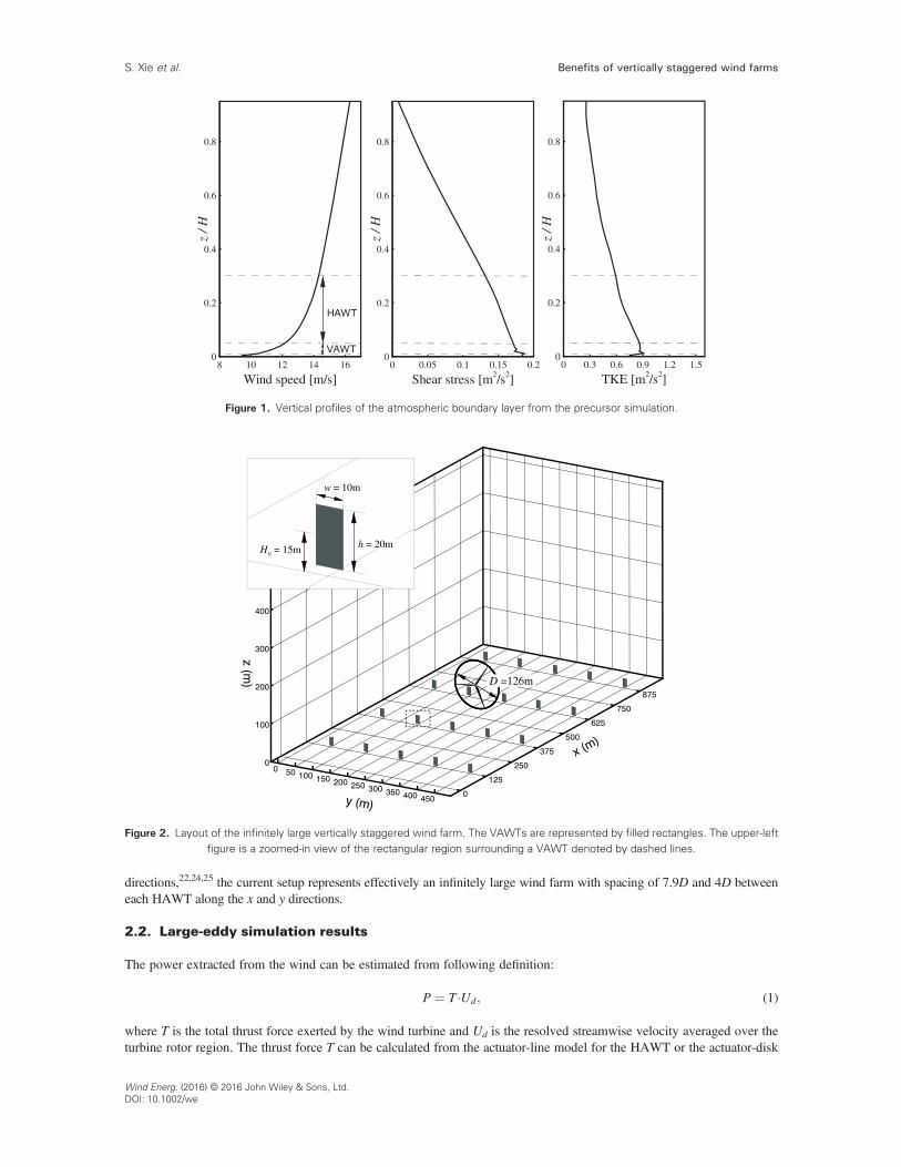
directions,22,24,25 the current setup represents effectively an infinitely large wind farm with spacing of 7.9D and 4D betweeneach HAWT along the x and y directions.

2.2. Large-eddy simulation results

The power extracted from the wind can be estimated from following definition:

P ¼ T #Ud; (1)

where T is the total thrust force exerted by the wind turbine and Ud is the resolved streamwise velocity averaged over theturbine rotor region. The thrust force T can be calculated from the actuator-line model for the HAWT or the actuator-disk

Figure 2. Layout of the infinitely large vertically staggered wind farm. The VAWTs are represented by filled rectangles. The upper-leftfigure is a zoomed-in view of the rectangular region surrounding a VAWT denoted by dashed lines.

Figure 1. Vertical profiles of the atmospheric boundary layer from the precursor simulation.

Benefits of vertically staggered wind farmsS. Xie et al.


model for the VAWTs. Note that equation 1 gives an estimation of power extracted from the wind, which is not the electricpower produced by the wind turbines. The extracted power is always higher than the generated power because of variouslosses, but the distinction is not important for the purposes of relative comparisons. Because we only simulate one periodiccell of turbines (1 HAWT plus 20 VAWTs for the VS wind farm, or 1 HAWT for the control wind farm) as a representationof the infinite wind farm, the power mentioned hereafter should be considered as ‘per cell’.

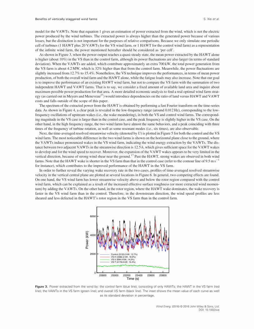
As shown in Figure 3, when the power output reaches a quasi-steady state, the mean power extracted by the HAWT aloneis higher (about 10%) in the VS than in the control farm, although its power fluctuations are also larger (in terms of standarddeviation). When the VAWTs are added, which contribute approximately an extra 700 kW, the total power generation fromthe VS farm is about 4.2MW, which is 32% higher than that from the control farm. Meanwhile, the power fluctuations areslightly increased from 12.7% to 15.4%. Nonetheless, the VS technique improves the performances, in terms of mean powerproduction, of both the overall wind farm and the HAWT alone, while the fatigue loads may also increase. Note that our goalis to improve the performance of an existing HAWT wind farm, but not to compare the VS farm with the summation of twoindependent HAWT and VAWT farms. That is to say, we consider a fixed amount of available land area and inquire aboutmaximum possible power production for that area. A more detailed economic analysis to find a real optimal wind farm strat-egy (as carried out inMeyers andMeneveau27) would introduce dependencies on the ratio of land versus HAWT and VAWTcosts and falls outside of the scope of this paper.

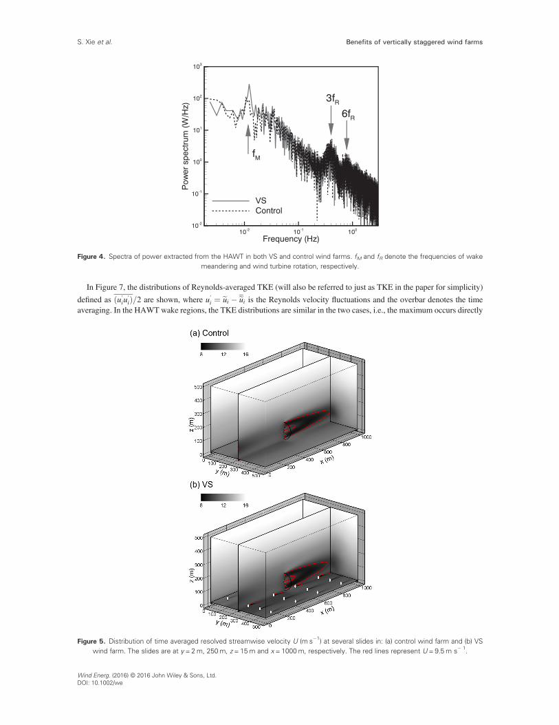
The spectrum of the extracted power from the HAWT is obtained by performing a fast Fourier transform on the time-seriesdata. As shown in Figure 4, a clear peak is revealed in the low-frequency range (around 0.012Hz), corresponding to the low-frequency oscillations of upstream wakes (i.e., the wake meandering), in both the VS and control wind farms. The correspond-ing magnitude in the VS case is larger than in the control case, and the peak frequency is slightly higher in the VS case. On theother hand, in the high frequency range, the two wind farms have almost the same behaviors, and a peak coinciding with threetimes of the frequency of turbine rotation, as well as some resonant modes (i.e., six times), are also observable.

Next, the time-averaged resolved streamwise velocity (denoted byU) is plotted in Figure 5 for both the control and the VSwind farm. The most noticeable difference in the two wind farms is shown on the horizontal plane close to the ground, wherethe VAWTs induce pronounced wakes in the VS wind farm, indicating the wind energy extraction by the VAWTs. The dis-tance between two adjacent VAWTs in the streamwise direction is 12.5 h, which gives sufficient space for the VAWTwakesto develop and for the wind speed to recover. Moreover, the expansion of the VAWTwakes appears to be very limited in thevertical direction, because of strong wind shear near the ground.17 Past the HAWT, strong wakes are observed in both windfarms. Note that the HAWT wake is shorter in the VS farm than that in the control case (refer to the contour line of 9.5m s!1

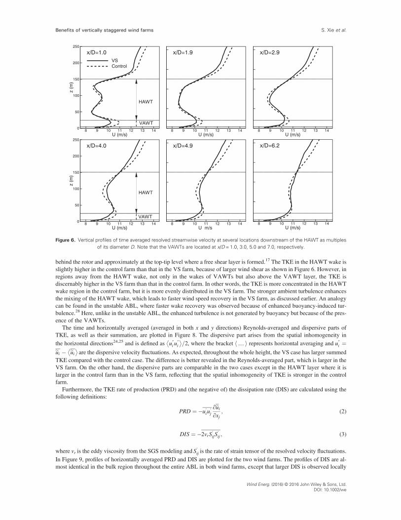
for instance), which contributes to the improved performance of the HAWT in the VS farm.In order to further reveal the varying wake recovery rate in the two cases, profiles of time-averaged resolved streamwise

velocity in the vertical central plane are plotted at several locations in Figure 6. In general, two competing effects are found.On one hand, the VS wind farm has lower streamwise velocity above and below the rotor region compared with the controlwind farm, which can be explained as a result of the increased effective surface roughness (or more extracted wind momen-tum) by adding the VAWTs. On the other hand, in the rotor region, where the HAWT wake dominates, the wake recovery isfaster in the VS wind farm than in the control. Therefore, in the downstream direction, the wind speed profiles are lesssheared and less defected in the HAWT’s rotor region in the VS farm than in the control farm.

Figure 3. Power extracted from the wind by: the control farm (blue line), consisting of only HAWTs; the HAWT in the VS farm (redline); the VAWTs in the VS farm (green line); and overall VS farm (black line). The inset shows the mean value of each curve as well

as its standard deviation in percentage.



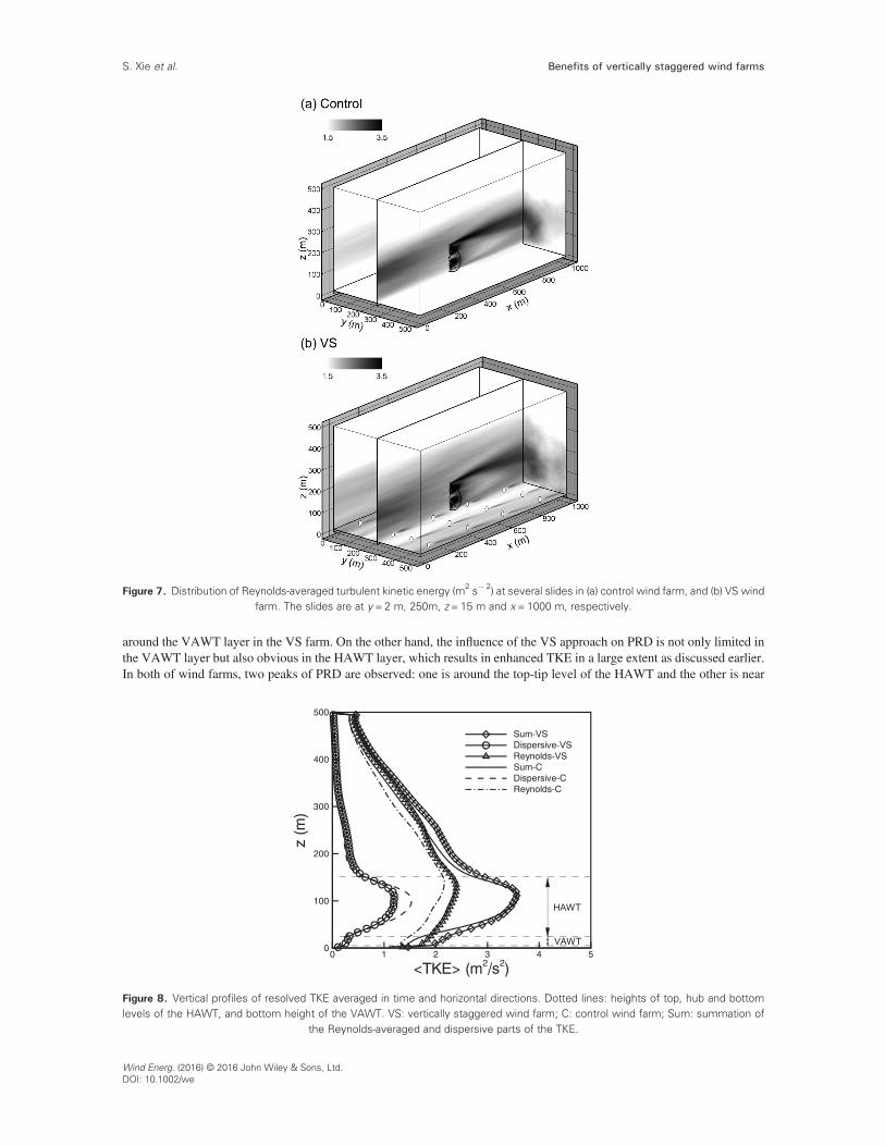
In Figure 7, the distributions of Reynolds-averaged TKE (will also be referred to just as TKE in the paper for simplicity)

defined as u′iu′ið Þ=2 are shown, where u′i ¼ eui ! eui is the Reynolds velocity fluctuations and the overbar denotes the time

averaging. In the HAWT wake regions, the TKE distributions are similar in the two cases, i.e., the maximum occurs directly

Figure 5. Distribution of time averaged resolved streamwise velocity U (m s!1) at several slides in: (a) control wind farm and (b) VSwind farm. The slides are at y = 2m, 250m, z = 15m and x= 1000m, respectively. The red lines represent U = 9.5m s! 1.

Figure 4. Spectra of power extracted from the HAWT in both VS and control wind farms. fM and fR denote the frequencies of wakemeandering and wind turbine rotation, respectively.



behind the rotor and approximately at the top-tip level where a free shear layer is formed.17 The TKE in the HAWT wake isslightly higher in the control farm than that in the VS farm, because of larger wind shear as shown in Figure 6. However, inregions away from the HAWT wake, not only in the wakes of VAWTs but also above the VAWT layer, the TKE isdiscernably higher in the VS farm than that in the control farm. In other words, the TKE is more concentrated in the HAWTwake region in the control farm, but it is more evenly distributed in the VS farm. The stronger ambient turbulence enhancesthe mixing of the HAWT wake, which leads to faster wind speed recovery in the VS farm, as discussed earlier. An analogycan be found in the unstable ABL, where faster wake recovery was observed because of enhanced buoyancy-induced tur-bulence.28 Here, unlike in the unstable ABL, the enhanced turbulence is not generated by buoyancy but because of the pres-ence of the VAWTs.

The time and horizontally averaged (averaged in both x and y directions) Reynolds-averaged and dispersive parts ofTKE, as well as their summation, are plotted in Figure 8. The dispersive part arises from the spatial inhomogeneity inthe horizontal directions24,25 and is defined as u″i u

″i

! "=2, where the bracket h… i represents horizontal averaging and u″i ¼

eui ! eui! "

are the dispersive velocity fluctuations. As expected, throughout the whole height, the VS case has larger summedTKE compared with the control case. The difference is better revealed in the Reynolds-averaged part, which is larger in theVS farm. On the other hand, the dispersive parts are comparable in the two cases except in the HAWT layer where it islarger in the control farm than in the VS farm, reflecting that the spatial inhomogeneity of TKE is stronger in the controlfarm.

Furthermore, the TKE rate of production (PRD) and (the negative of) the dissipation rate (DIS) are calculated using thefollowing definitions:

PRD ¼ !u′iu′j∂eui∂xj

; (2)

DIS ¼ !2νrS′ijS′ij ; (3)

where νr is the eddy viscosity from the SGS modeling and S′ij is the rate of strain tensor of the resolved velocity fluctuations.In Figure 9, profiles of horizontally averaged PRD and DIS are plotted for the two wind farms. The profiles of DIS are al-most identical in the bulk region throughout the entire ABL in both wind farms, except that larger DIS is observed locally

Figure 6. Vertical profiles of time averaged resolved streamwise velocity at several locations downstream of the HAWT as multiplesof its diameter D. Note that the VAWTs are located at x/D = 1.0, 3.0, 5.0 and 7.0, respectively.



around the VAWT layer in the VS farm. On the other hand, the influence of the VS approach on PRD is not only limited inthe VAWT layer but also obvious in the HAWT layer, which results in enhanced TKE in a large extent as discussed earlier.In both of wind farms, two peaks of PRD are observed: one is around the top-tip level of the HAWT and the other is near

Figure 7. Distribution of Reynolds-averaged turbulent kinetic energy (m2 s! 2) at several slides in (a) control wind farm, and (b) VS windfarm. The slides are at y = 2 m, 250m, z = 15 m and x= 1000 m, respectively.

Figure 8. Vertical profiles of resolved TKE averaged in time and horizontal directions. Dotted lines: heights of top, hub and bottomlevels of the HAWT, and bottom height of the VAWT. VS: vertically staggered wind farm; C: control wind farm; Sum: summation of

the Reynolds-averaged and dispersive parts of the TKE.



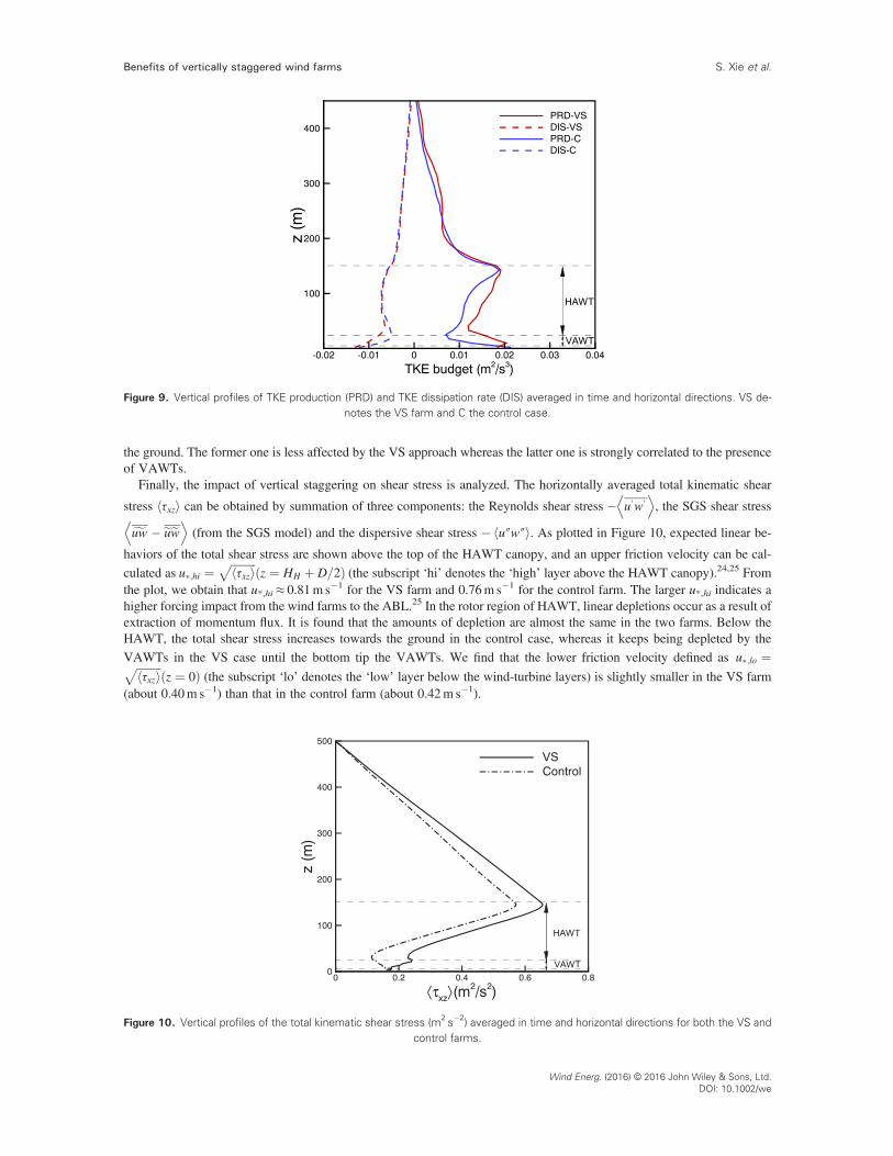
the ground. The former one is less affected by the VS approach whereas the latter one is strongly correlated to the presenceof VAWTs.

Finally, the impact of vertical staggering on shear stress is analyzed. The horizontally averaged total kinematic shear

stress hτxzi can be obtained by summation of three components: the Reynolds shear stress ! u′w′D E

, the SGS shear stress

fuw ! euewD E

(from the SGS model) and the dispersive shear stress ! hu″w″i. As plotted in Figure 10, expected linear be-

haviors of the total shear stress are shown above the top of the HAWT canopy, and an upper friction velocity can be cal-culated as u&;hi ¼

ffiffiffiffiffiffiffiffiffiτxzh i

pz ¼ HH þ D=2ð Þ (the subscript ‘hi’ denotes the ‘high’ layer above the HAWT canopy).24,25 From

the plot, we obtain that u*,hi≈ 0.81m s!1 for the VS farm and 0.76m s!1 for the control farm. The larger u*,hi indicates ahigher forcing impact from the wind farms to the ABL.25 In the rotor region of HAWT, linear depletions occur as a result ofextraction of momentum flux. It is found that the amounts of depletion are almost the same in the two farms. Below theHAWT, the total shear stress increases towards the ground in the control case, whereas it keeps being depleted by theVAWTs in the VS case until the bottom tip the VAWTs. We find that the lower friction velocity defined as u&;lo ¼ffiffiffiffiffiffiffiffiffi

τxzh ip

z ¼ 0ð Þ (the subscript ‘lo’ denotes the ‘low’ layer below the wind-turbine layers) is slightly smaller in the VS farm(about 0.40m s!1) than that in the control farm (about 0.42m s!1).

Figure 9. Vertical profiles of TKE production (PRD) and TKE dissipation rate (DIS) averaged in time and horizontal directions. VS de-notes the VS farm and C the control case.

Figure 10. Vertical profiles of the total kinematic shear stress (m2 s!2) averaged in time and horizontal directions for both the VS andcontrol farms.



3. ANALYTICAL MODEL

3.1. Model description

Numerous low-order models are available to study the wind farm wakes, each focusing on different aspects of the prob-lem.26,29–32 Following the assumption of infinitely large, fully developed wind farm as in the previous section, an analytical‘top-down’ model, primarily developed by Frandsen33,34 and Calaf et al.24 and later extended to a large but finite-size windfarms by Meneveau,35 was modified here to take into account the vertical staggering and addition of VAWT.

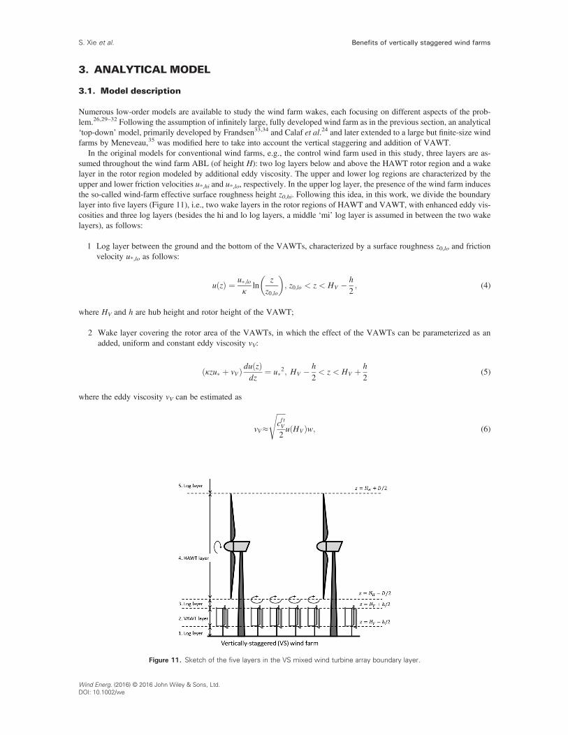
In the original models for conventional wind farms, e.g., the control wind farm used in this study, three layers are as-sumed throughout the wind farm ABL (of height H): two log layers below and above the HAWT rotor region and a wakelayer in the rotor region modeled by additional eddy viscosity. The upper and lower log regions are characterized by theupper and lower friction velocities u*,hi and u*,lo, respectively. In the upper log layer, the presence of the wind farm inducesthe so-called wind-farm effective surface roughness height z0,hi. Following this idea, in this work, we divide the boundarylayer into five layers (Figure 11), i.e., two wake layers in the rotor regions of HAWT and VAWT, with enhanced eddy vis-cosities and three log layers (besides the hi and lo log layers, a middle ‘mi’ log layer is assumed in between the two wakelayers), as follows:

1 Log layer between the ground and the bottom of the VAWTs, characterized by a surface roughness z0,lo and frictionvelocity u*,lo as follows:

u zð Þ ¼ u&;loκ

lnz

z0;lo

$ %; z0;lo < z < HV ! h

2; (4)

where HV and h are hub height and rotor height of the VAWT;

2 Wake layer covering the rotor area of the VAWTs, in which the effect of the VAWTs can be parameterized as anadded, uniform and constant eddy viscosity νV:

κzu& þ νVð Þ du zð Þdz

¼ u&2; HV ! h2< z < HV þ h

2(5)

where the eddy viscosity νV can be estimated as

νV≈

ffiffiffiffifficf tV2

s

u HVð Þw; (6)

Figure 11. Sketch of the five layers in the VS mixed wind turbine array boundary layer.



whereffiffiffiffiffiffiffiffiffifficf tV=2

qu HVð Þ is a characteristic velocity scale due to momentum defect, and w is the relevant characteristic length

scale (as the integral length scale of vortices from a VAWT are of the order of the rotor diameter). Equation 5 can berewritten as

1þ ν&V& ' du zð Þ

dln zHV

( ) ¼ u&κ; (7)

where ν&V is the effective eddy viscosity estimated as

ν&V ¼ νVκu&z

: (8)

Further in equation 6, cf tV is the loading coefficient of the VAWT,24,25,35 which is a function of the thrust coefficient CVT,

the rotor area of the VAWTs AV and the horizontal spacing between VAWTs in the streamwise and spanwise direc-tions SxV and SyV

cf tV ¼ CVTAV

SxVSyV¼ CV

T hwSxVS

yV: (9)

The effective added viscosity ν&V is evaluated at HV and is no longer a function of z,24 and the choice of the respectivefriction velocity u* will be discussed shortly;

3 Log layer between the top of the VAWTs and the lower tip of the larger HAWTs, characterized by z0,mi and u*,mi:

u zð Þ ¼ u&;miκ

lnz

z0;mi

$ %; HV þ h

2< z < HH ! D

2; (10)

where HH and D are hub height and diameter of the HAWT;

4 Wake layer covering the rotor area of the large HAWTs, in which again the effect of the wind turbine is parameterizedas an added, uniform and constant eddy viscosity νH:

1þ ν&H& ' du zð Þ

dln zHH

( ) ¼ u&κ; HH ! D

2< z < HH þ D

2; (11)

where

ν&H ¼ νHκu&HH

; and νH≈

ffiffiffiffifficf tH2

s

u HHð ÞD (12)

cf tH ¼ CHT AH

SxHSyH

¼ CHT πD

2

4SxHSyH; (13)

5 Log layer above the HAWTs with z0,hi and u*,hi

u zð Þ ¼ u&;hiκ

lnz

z0;hi

$ %; HH þ D

2< z < H: (14)

Next, with the earlier assumptions, we derive analytical expressions for wind speed at the respective hubheights of the VAWTs and HAWTs. Focusing first on layer 2, equation 7 can be integrated in the vertical direc-tion by matching the velocities at the top and bottom of the layer to those in layer 1 and 3, respectively, to obtainthe following:



u zð Þ ¼ u&;loκ

lnzHV

$ % 11þν&

V ;l HV

z0;lo

$ %HV ! h

2

HV

$ % ν&V ;l

1þν&V ;l

2

64

3

75; HV ! h2≤z < HV ; (15)

u zð Þ ¼ u&;miκ

lnzHV

$ % 11þν&

V ;u HV

z0;mi

$ %HV þ h

2

HV

$ % ν&V ;u

1þν&V ;u

2

64

3

75; HV≤z < HV þ h2; (16)

where ν&V ;l ¼νV

κHVu&;loand ν&V ;u ¼

νVκHVu&;mi

are used below and above the hub height of the VAWT, respectively, and νVis given by equation 6. As a result, at hub height HV

u HVð Þ ¼ u&;loκ

lnHV

z0;lo

$ %HV ! h

2

$ % ν&V ;l

1þν&V ;l

2

4

3

5 ¼ u&;miκ

lnHV

z0;mi

$ %HV þ h

2

$ % ν&V ;u

1þν&V ;u

2

4

3

5: (17)

From the momentum balance33,35

u2&;mi ¼ u2&;lo þ12cf tV u HVð Þ2; (18)

u2&;hi ¼ u2&;mi þ12cf tHu HHð Þ2; (19)

and from equation 17, we have

u&;miu*;lo

¼ln HV

z0;lo

( )þ ν&V ;l

1þν&V ;lln HV!h

2HV

( )

ln HVz0;mi

( )þ ν&V ;u

1þν&V ;uln HVþh

2HV

( ) : (20)

Substituting equations 17 and 20 into equation 18, an analytical expression for z0,mi can be obtained:

z0;mi ¼ HVHV þ h

2

HV

$ % ν&V ;u

1þν&V ;uexp ! cf tV

2κ2þ ln

HV

z0;lo

HV ! h2

HV

$ % ν&V ;l

1þν&V ;l

2

64

3

75

8><

>:

9>=

>;

!22

64

3

75

!1=2

0

BBB@

1

CCCA: (21)

Note that ν&V ;l and ν&V ;u are unknown, and they are dependent on z0,mi, u*,mi and u*,lo. A simple iteration method isused to solve them by initially setting z0,mi = z0 and u*,lo = u*,mi = u*. Similarly for level 4, with the HAWT, thefollowing relationships are obtained:

u HHð Þ ¼ u&;hiκ

lnHH

z0;hi

$ %HH þ D

2

$ % ν&H;u

1þν&H;u

2

4

3

5 ¼ u&;miκ

lnHH

z0;mi

$ %HH ! D

2

$ % ν&H;l

1þν&H;l

2

4

3

5 (22)

u&;hiu&;mi

¼ln HH

z0;mi

( )þ ν&H;l

1þν&H;lln HH!D

2HH

( )

ln HHz0;hi

( )þ ν&H;u

1þν&H;uln HHþD

2HH

( ) (23)



z0;hi ¼ HHHH þ D

2

HH

$ % ν&H;u

1þν&H;uexp ! cf tH

2κ2þ ln

HH

z0;mi

HH ! D2

HH

$ % ν&H;l

1þν&H;l

2

64

3

75

8><

>:

9>=

>;

!22

64

3

75

!1=2

0

BBB@

1

CCCA (24)

where ν&H;l ¼νH

κHHu&;miand ν&H;u ¼

νHκHHu&;hi

, and νH is given by equation 12. Now, the only unknown is u*,hi, which can

be derived from the geostrophic relationship:

u&;hi ¼κUG

ln UGf z0;hi

( )! C

; (25)

where C ~ 4.5 is a standard empirical value for neutral ABL,35 UG is the geostrophic wind speed and f is the Coriolisparameter. Here, because the Coriolis forcing is not considered, equation 25 can be simplified as follows:

u&;hi ¼κUG

ln HGz0;hi

( ) ; (26)

where HG is the boundary layer height where UG is imposed. In Appendix A, a flowchart summarizing the model isprovided in Figure 15. Note that it is not necessary to have the intermediate log layer between the VAWTs andHAWTs (i.e., the third layer), when the top-tip level of the VAWTs and bottom tip level of the HAWTs are coinci-dent (although no overlap between the two rotor regions is permitted). However, as in Section 2, z0,mi and u*,mi arestill calculated as described earlier and used in the equations of the other parameters.

3.2. Analytical results of the VS wind farm

In this section, the performance of the VS wind farm is evaluated using the analytical top-down model described earlier.From the LES results in Section 2.2, the thrust coefficients of the HAWT were found to be CH

T≈0:59 in the VS case and0.54 in the control case. Note that the determination of the thrust coefficient is sensitive to the choice of upstream referencevelocity. Here, the streamwise velocity at D/2 in front of the HAWT averaged over the rotor region was used. FollowingStevens et al.,36 an effective spacing in the lateral direction Syeff should be used instead of Sy in equations 9 and 13, in orderto produce the correct wake expansion. In principle, the effective spacing has to be determined by matching the top-downmodel with a wake model, which is outside the scope of the current modeling effort. For the configuration in this study, wefound empirically that the following values

SyH;eff ¼ 2:5D (27)

SyV ;eff ¼ 4:0w (28)

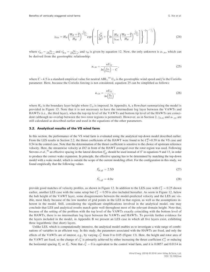
provide good matches of velocity profiles, as shown in Figure 12. In addition to the LES case with CVT ¼ 0:25 shown

earlier, another LES case with the same setup but CVT ¼ 0:50 is also included hereafter. As seem in Figure 12, below

the hub height of the VAWT layer, some disagreements between the model-predicted velocity and the LES are vis-ible, most likely because of the low number of grid points in the LES in that region, as well as the assumptions in-herent in the model. Still, considering the significant simplifications involved in the analytical model, one mayconclude that LES and analytical results match quite well throughout most of the relevant domain height. Note that,because of the setting of the problem with the top level of the VAWTs exactly coinciding with the bottom level ofthe HAWTs, there is no intermediate log layer between the VAWTs and HAWTs. To provide further evidence forthe layers included in the model, in Appendix B we present an LES case in which all five layers exist, exhibitingthree logarithmic (but short) layers.

Unlike LES, which is computationally intensive, the analytical model enables us to investigate a wide range of combi-nations of variables in an efficient way. In this study, the parameters associated with the HAWTs are fixed, and only theeffects of the VAWTs are of interest, e.g., by varying cf tV from 0 to 0.05 (Figure 13). Here, the height and rotor area ofthe VAWT are fixed, so the change of cf tV is primarily achieved by either increasing the thrust coefficient CV

T or reducing

the horizontal spacing SxV or SyV . Note that cf tV ¼ 0 is equivalent to the control wind farm, and it is 0.0057 and 0.0114 in



the LES with CVT ¼ 0:25 and CV

T ¼ 0:50, respectively. While only two LES cases are presented in this paper, we find thatthe LES results agree well with the analytical model.

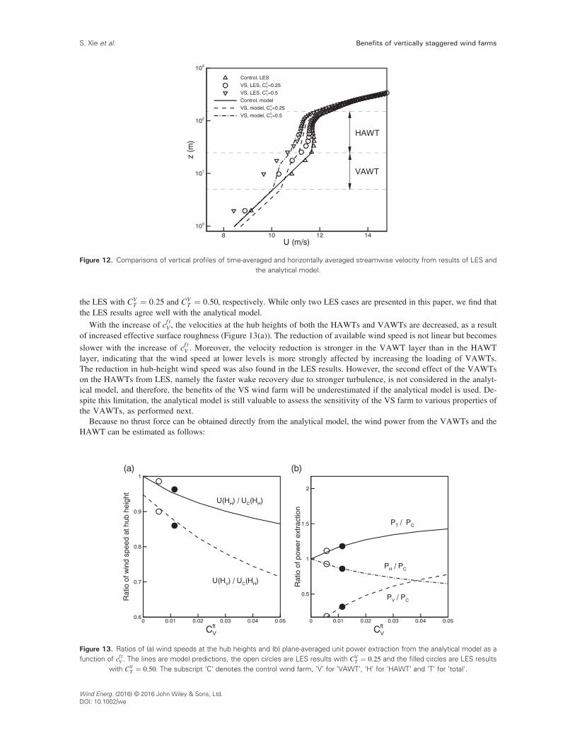
With the increase of cf tV , the velocities at the hub heights of both the HAWTs and VAWTs are decreased, as a resultof increased effective surface roughness (Figure 13(a)). The reduction of available wind speed is not linear but becomesslower with the increase of cf tV . Moreover, the velocity reduction is stronger in the VAWT layer than in the HAWTlayer, indicating that the wind speed at lower levels is more strongly affected by increasing the loading of VAWTs.The reduction in hub-height wind speed was also found in the LES results. However, the second effect of the VAWTson the HAWTs from LES, namely the faster wake recovery due to stronger turbulence, is not considered in the analyt-ical model, and therefore, the benefits of the VS wind farm will be underestimated if the analytical model is used. De-spite this limitation, the analytical model is still valuable to assess the sensitivity of the VS farm to various properties ofthe VAWTs, as performed next.

Because no thrust force can be obtained directly from the analytical model, the wind power from the VAWTs and theHAWT can be estimated as follows:

Figure 12. Comparisons of vertical profiles of time-averaged and horizontally averaged streamwise velocity from results of LES andthe analytical model.

Figure 13. Ratios of (a) wind speeds at the hub heights and (b) plane-averaged unit power extraction from the analytical model as afunction of cf tV . The lines are model predictions, the open circles are LES results with CV

T ¼ 0:25 and the filled circles are LES resultswith CV

T ¼ 0:50. The subscript ‘C’ denotes the control wind farm, ‘V’ for ‘VAWT’, ‘H’ for ‘HAWT’ and ‘T’ for ‘total’.



PV ¼ 12ρac

f tV u HVð Þh i3; (29)

PH ¼ 12ρac

f tH u HHð Þh i3; (30)

where ρa is the air density. The power calculated here is not the same as the power shown in Figure 3, because this is ac-tually power per horizontal unit area around the turbine clear of turbines of the same type (note that SxHS

yH;eff and S

xHS

yH;eff are

in the denominator of the definition of cf tH and cf tV , respectively), and the plane-averaged velocity at hub height hū(HH)i orhū(HV)i is used instead of Ud. Thus, we use the term ‘plane-averaged unit power’ (or just unit power for simplicity) here todistinguish among these concepts. We found that the slight decrease in PH with cf tV is more than compensated for by PV (Figure 13(b)), and therefore, the total PT=PH+PV increases with cf tV in the range considered here. Consistent with the ve-locity variations at the hub heights, the changes in the total unit power become more gentle with larger cf tV . Intuitively, theincrease of VAWT loading may not always be beneficial to the overall farm performance, because the aloft wind speedcould be reduced to the point that the energy loss by the large turbines may not be compensated by the gain from VAWTs.A maximum power ratio of 1.5 in the VS wind farm is found at cf tV≈0:12, but it is not shown here because of lack of LESdata for validation.

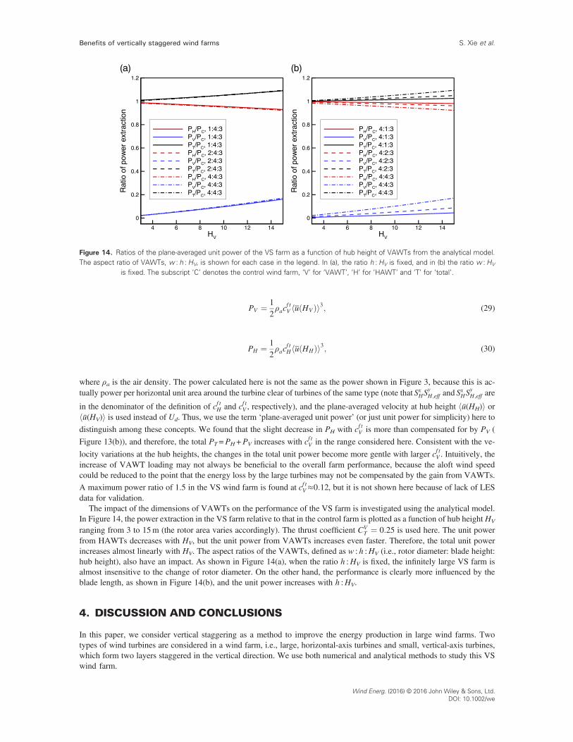
The impact of the dimensions of VAWTs on the performance of the VS farm is investigated using the analytical model.In Figure 14, the power extraction in the VS farm relative to that in the control farm is plotted as a function of hub height HV

ranging from 3 to 15m (the rotor area varies accordingly). The thrust coefficient CVT ¼ 0:25 is used here. The unit power

from HAWTs decreases with HV, but the unit power from VAWTs increases even faster. Therefore, the total unit powerincreases almost linearly with HV. The aspect ratios of the VAWTs, defined as w : h :HV (i.e., rotor diameter: blade height:hub height), also have an impact. As shown in Figure 14(a), when the ratio h :HV is fixed, the infinitely large VS farm isalmost insensitive to the change of rotor diameter. On the other hand, the performance is clearly more influenced by theblade length, as shown in Figure 14(b), and the unit power increases with h :HV.

4. DISCUSSION AND CONCLUSIONS

In this paper, we consider vertical staggering as a method to improve the energy production in large wind farms. Twotypes of wind turbines are considered in a wind farm, i.e., large, horizontal-axis turbines and small, vertical-axis turbines,which form two layers staggered in the vertical direction. We use both numerical and analytical methods to study this VSwind farm.

Figure 14. Ratios of the plane-averaged unit power of the VS farm as a function of hub height of VAWTs from the analytical model.The aspect ratio of VAWTs, w : h :HV, is shown for each case in the legend. In (a), the ratio h :HV is fixed, and in (b) the ratio w :HV

is fixed. The subscript ‘C’ denotes the control wind farm, ‘V’ for ‘VAWT’, ‘H’ for ‘HAWT’ and ‘T’ for ‘total’.



For the LES, periodic boundary conditions are used in all horizontal directions to mimic an infinite wind farm, an ide-alized condition in which transport and variability from flow scales larger than the domain size are neglected. The VS farmis compared with a conventional layout with only HAWTs (control farm). We find that the VS farm, with 20 VAWTsaround each HAWT, can extract about 32% more power from the wind than the control wind farm and that the powerextracted by the HAWT alone is also increased by about 10%. Because of the presence of the VAWT layer, the turbulencein the wind farm is increased, which enhances the wake recovery of the HAWT. The faster wake recovery more thancompensates for the additional momentum loss in the wind because of increased effective surface roughness associatedwith the VAWTs.

A theoretical top-down model is developed for the infinite, fully developed, VS wind farm, in which five distinct layers(three log layers and two wake layers) are assumed to form throughout the boundary layer. The results show that the totalmomentum loss increases with either an increase of the thrust coefficient or a decrease of the spacing between VAWTs, theratio of which is called the loading coefficient. Moreover, the analytical model shows that the total power increases with theloading coefficient in the range close to the LES configurations, but a maximum power may be reached at some highloading values. The sensitivity of the dimensions of VAWTs is studied by the analytical model as well, which indicatesthat, when the thrust coefficient is fixed, the total power increases almost linearly with the height of VAWTs while it isnot sensitive to the width of the rotor.

Furthermore, it is helpful to compare the VS approach with the conventional approach of adding more HAWTs. Byadding another 5 MW HAWT in the x direction in the same domain, the distance between two HAWTs is reduced by half,e.g., from 8D to 4D, which leads to a wake loss of about 33% (averaged over all wind directions, such as showed for theLillgrund wind farm37) for each turbine. Therefore, the total power of two HAWTs is roughly 6.7MW, which is higher thanthe current LES result of the VS farm (4.2MW). However, the capital cost of a 5 MW turbine is roughly $10m, whiletwenty 50 kW VAWTs cost about $5m.38 Therefore, the VS approach has a better capital cost per MW than the conven-tional one (1.19 vs. 1.49). Therefore, adding more HAWTs may be less beneficial than adding VAWT although the eco-nomically optimal arrangement depends upon capital and operating costs as well as the price of energy and land costs.

Despite the great potential shown in this study, there are still numerous issues that are not addressed here but will beincluded in our future research. It is more realistic from the application point of view to study finite-size wind farms withboth LES and the analytical model. The atmospheric stability should be considered, which strongly influences the turbu-lence in the ABL and hence wake properties.28 Moreover, the VAWT wakes should be simulated using more sophisticatedmodels, e.g., the actuator-line model, which leads to a better understanding of the wake interactions and possibly to the op-timization of the VAWT placement. It is also important to assess the sensitivity of the VS wind farm to changes in winddirection. Even though it is known that even slight misalignments between the orientation of the rows and columns of tur-bines and the wind direction can lead to large differences in wake losses and therefore power output, it is expected thatadding VAWTs will still be beneficial at the end, after considering all wind directions. The effect of wind direction onVS farms is likely to be different from the effect on traditional wind farms composed of only HAWTs and needs to be stud-ied in future. In addition, considering the small size and low height of the VAWTs, their performance may be influenced bythe wake effects from the tower of the HAWT, which is not considered in this study. Last but not least, as mentioned earlier,an economic analysis is needed to evaluate the actual revenue that can be generated annually or over the lifetime of thewind farm by using vertical staggering.

ACKNOWLEDGEMENT

This research was supported in part by the National Science Foundation (Grants No. 1357649 and IIA-1243482).



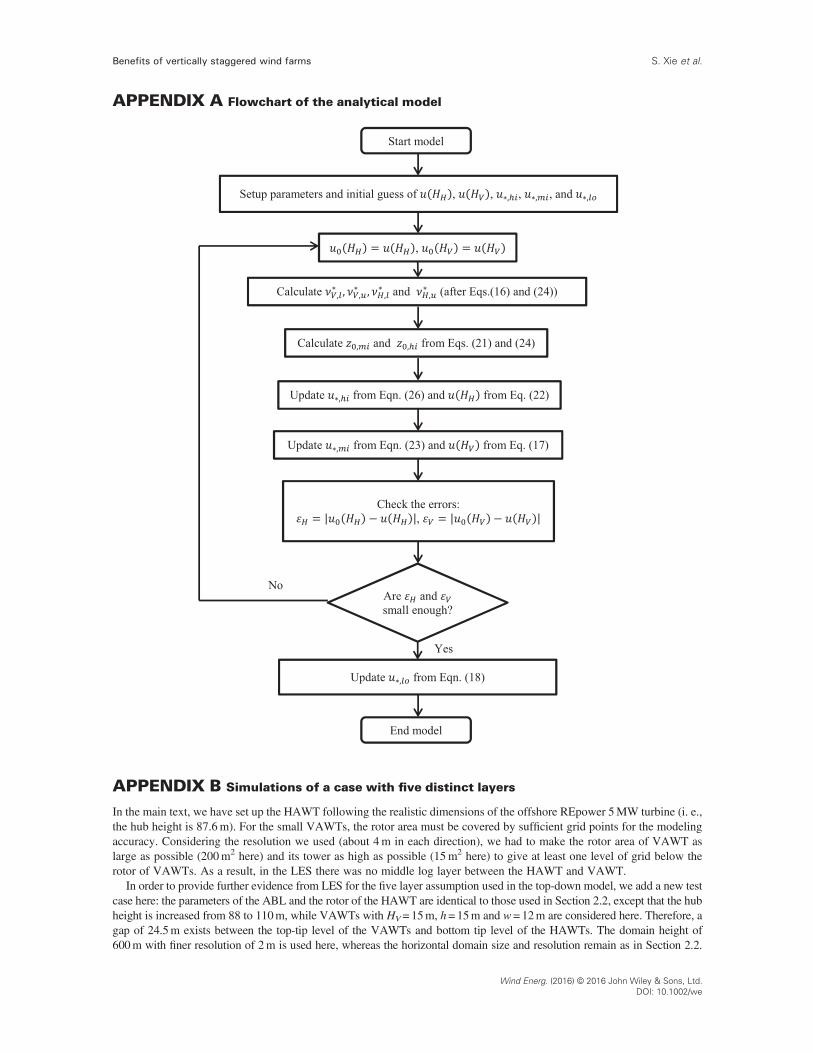
APPENDIX A Flowchart of the analytical model

APPENDIX B Simulations of a case with five distinct layers

In the main text, we have set up the HAWT following the realistic dimensions of the offshore REpower 5MW turbine (i. e.,the hub height is 87.6m). For the small VAWTs, the rotor area must be covered by sufficient grid points for the modelingaccuracy. Considering the resolution we used (about 4m in each direction), we had to make the rotor area of VAWT aslarge as possible (200m2 here) and its tower as high as possible (15m2 here) to give at least one level of grid below therotor of VAWTs. As a result, in the LES there was no middle log layer between the HAWT and VAWT.

In order to provide further evidence from LES for the five layer assumption used in the top-down model, we add a new testcase here: the parameters of the ABL and the rotor of the HAWT are identical to those used in Section 2.2, except that the hubheight is increased from 88 to 110m, while VAWTs with HV=15m, h=15m and w=12m are considered here. Therefore, agap of 24.5m exists between the top-tip level of the VAWTs and bottom tip level of the HAWTs. The domain height of600m with finer resolution of 2m is used here, whereas the horizontal domain size and resolution remain as in Section 2.2.



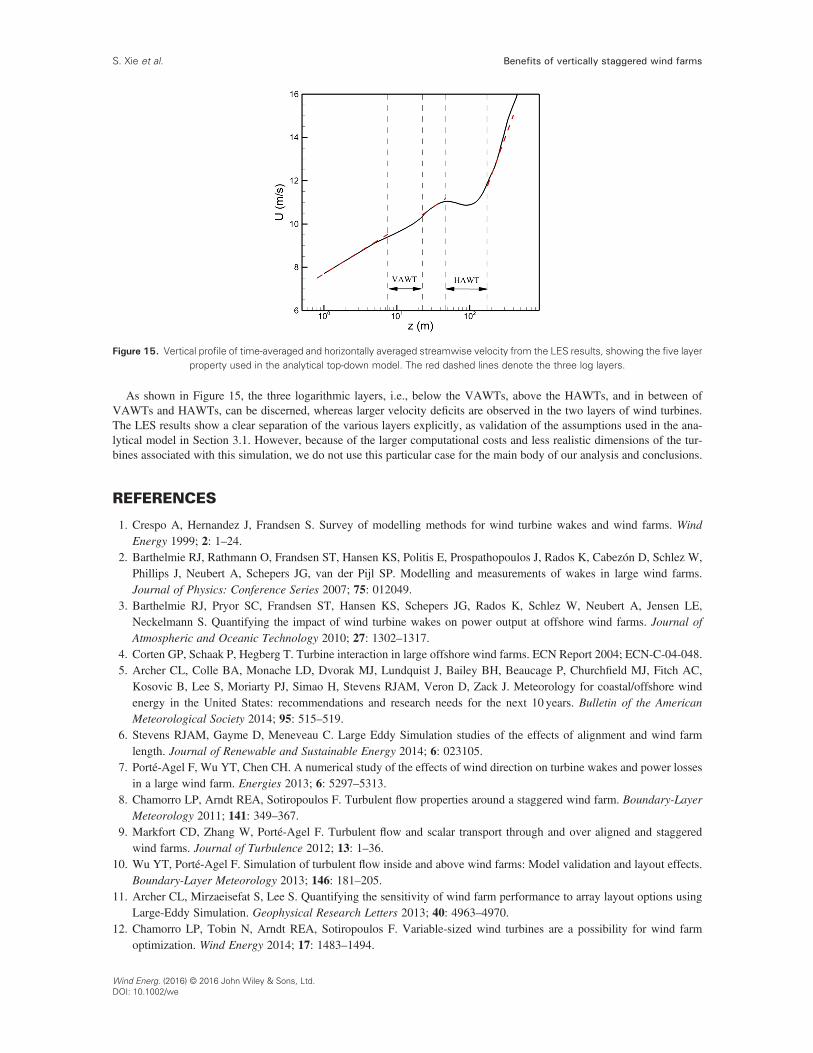
As shown in Figure 15, the three logarithmic layers, i.e., below the VAWTs, above the HAWTs, and in between ofVAWTs and HAWTs, can be discerned, whereas larger velocity deficits are observed in the two layers of wind turbines.The LES results show a clear separation of the various layers explicitly, as validation of the assumptions used in the ana-lytical model in Section 3.1. However, because of the larger computational costs and less realistic dimensions of the tur-bines associated with this simulation, we do not use this particular case for the main body of our analysis and conclusions.

REFERENCES

1. Crespo A, Hernandez J, Frandsen S. Survey of modelling methods for wind turbine wakes and wind farms. WindEnergy 1999; 2: 1–24.

2. Barthelmie RJ, Rathmann O, Frandsen ST, Hansen KS, Politis E, Prospathopoulos J, Rados K, Cabezón D, Schlez W,Phillips J, Neubert A, Schepers JG, van der Pijl SP. Modelling and measurements of wakes in large wind farms.Journal of Physics: Conference Series 2007; 75: 012049.

3. Barthelmie RJ, Pryor SC, Frandsen ST, Hansen KS, Schepers JG, Rados K, Schlez W, Neubert A, Jensen LE,Neckelmann S. Quantifying the impact of wind turbine wakes on power output at offshore wind farms. Journal ofAtmospheric and Oceanic Technology 2010; 27: 1302–1317.

4. Corten GP, Schaak P, Hegberg T. Turbine interaction in large offshore wind farms. ECN Report 2004; ECN-C-04-048.5. Archer CL, Colle BA, Monache LD, Dvorak MJ, Lundquist J, Bailey BH, Beaucage P, Churchfield MJ, Fitch AC,

Kosovic B, Lee S, Moriarty PJ, Simao H, Stevens RJAM, Veron D, Zack J. Meteorology for coastal/offshore windenergy in the United States: recommendations and research needs for the next 10 years. Bulletin of the AmericanMeteorological Society 2014; 95: 515–519.

6. Stevens RJAM, Gayme D, Meneveau C. Large Eddy Simulation studies of the effects of alignment and wind farmlength. Journal of Renewable and Sustainable Energy 2014; 6: 023105.

7. Porté-Agel F, Wu YT, Chen CH. A numerical study of the effects of wind direction on turbine wakes and power lossesin a large wind farm. Energies 2013; 6: 5297–5313.

8. Chamorro LP, Arndt REA, Sotiropoulos F. Turbulent flow properties around a staggered wind farm. Boundary-LayerMeteorology 2011; 141: 349–367.

9. Markfort CD, Zhang W, Porté-Agel F. Turbulent flow and scalar transport through and over aligned and staggeredwind farms. Journal of Turbulence 2012; 13: 1–36.

10. Wu YT, Porté-Agel F. Simulation of turbulent flow inside and above wind farms: Model validation and layout effects.Boundary-Layer Meteorology 2013; 146: 181–205.

11. Archer CL, Mirzaeisefat S, Lee S. Quantifying the sensitivity of wind farm performance to array layout options usingLarge-Eddy Simulation. Geophysical Research Letters 2013; 40: 4963–4970.

12. Chamorro LP, Tobin N, Arndt REA, Sotiropoulos F. Variable-sized wind turbines are a possibility for wind farmoptimization. Wind Energy 2014; 17: 1483–1494.

Figure 15. Vertical profile of time-averaged and horizontally averaged streamwise velocity from the LES results, showing the five layerproperty used in the analytical top-down model. The red dashed lines denote the three log layers.



13. Vested MH, Hamilton N, Sørensen JN, Cal RB. Wake interaction and power production of variable height model windfarms. Journal of Physics: Conference Series 2014; 524: 012169.

14. Dabiri JO, Greer JR, Koseff JR, Moin P, Peng J. A new approach to wind energy: opportunities and challenges. AIPConference Proceedings 2015; 1652: 51–57.

15. Kinzel M, Mulligan Q, Dabiri J. Energy exchange in an array of vertical-axis wind turbines. Journal of Turbulence2012; 13: 1–13.

16. Pope SB. Turbulent Flows. Cambridge University Press: New York, 2000; 558.17. Xie S, Archer CL. Self-similarity and turbulence characteristics of wind turbine wakes via large-eddy simulation.Wind

Energy 2015; 18: 1815–1838.18. Orszag SA. On the elimination of aliasing in finite-difference schemes by filtering high-wavenumber components.

Journal of Atmospheric Science 1971; 28: 1074–1074.19. Bou-Zeid E, Parlange MB, Meneveau C. A scale-dependent Lagrangian dynamic model for large eddy simulation of

complex turbulent flows. Physics of Fluids 2005; 17: 025105.20. Sørensen JN, Shen WZ. Numerical modeling of wind turbine wakes. Journal of Fluids Engineering 2002; 124: 393–399.21. Xie S, Ghaisas N, Archer CL. Sensitivity issues in finite-difference large-eddy simulations of the atmospheric boundary

layer. Boundary-Layer Meteorology 2015; 157: 421–445.22. Lu H, Porté-Agel F. Large-eddy simulation of a very large wind farm in a stable atmospheric boundary layer. Physics

of Fluids 2011; 23: 065101.23. Sutherland HJ, Berg DE, Thomas D. Ashwill TD. A retrospective of VAWT technology. Sandia Report; SAND2012-

0304, January 2012.24. Calaf M, Meneveau C, Meyers J. Large eddy simulation study of fully developed wind-turbine array boundary layers.

Physics of Fluids 2010; 22: 015110.25. Calaf M, Parlange MB, Meneveau C. Large eddy simulation study of scalar transport in fully developed wind turbine

array boundary layers. Physics of Fluids 2011; 23: 126603.26. Araya DB, Craig AE, Kinzel M, Dabiri JO. Low-order modeling of wind farm aerodynamics using leaky Rankine

bodies. Journal of Renewable and Sustainable Energy 2014; 6: 063118.27. Meyers J, Meneveau C. Optimal turbine spacing in fully developed wind farm boundary layers.Wind Energy 2012; 15:

305–317.28. Abkar M, Porté-Agel F. Influence of atmospheric stability on wind-turbine wakes: a large-eddy simulation study. Phys-

ics of Fluids 2015; 27: 035104.29. Abkar M, Porté-Agel F. A new wind-farm parameterization for large-scale atmospheric models. Journal of Renewable

and Sustainable Energy 2015; 7: 013121.30. Fitch AC, Olson JB, Lundquist JK, Dudhia J, Gupta AK, Michalakes J, Barstad I. Local and mesoscale impacts of wind

farms as parameterized in a mesoscale NWP model. Monthly Weather Review 2012; 140: 3017.31. Yang X, Sotiropoulos F. Analytical model for predicting the performance of arbitrary size and layout wind farms.Wind

Energy 2015. DOI: 10.1002/we.1894.32. Ghaisas N, Archer CL. Geometry-based models for studying the effects of wind farm layout. Journal of Atmospheric

and Oceanic Technology 2015. DOI: 10.1175/JTECH-D-14-00199.1.33. Frandsen S. On the wind speed reduction in the center of large clusters of wind turbines. Journal of Wind Engineering

and Industrial Aerodynamics 1992; 39: 251–265.34. Frandsen S, Barthelmie R, Pryor S, Rathmann O, Larsen S, Hojstrup J, Thogersen M. Analytical modelling of wind

speed deficit in large offshore wind farms. Wind Energy 2006; 9: 39–53.35. Meneveau C. The top-down model of wind farm boundary layers and its applications. Journal of Turbulence 2012; 13:

1–12.36. Stevens RJAM, Gayme D, Meneveau C. Coupled wake boundary layer model of wind-farms. Journal of Renewable

and Sustainable Energy 2015; 7: 023155.37. Dahlberg J-Å. Assessment of the Lillgrund windfarm: power performance wake effects. Vattenfall Vindkraft AB, 6_1

LG Pilot Report, Sept. 2009. URL: https://corporate.vattenfall.se/globalassets/sverige/om-vattenfall/om-oss/var-verksamhet/vindkraft/lillgrund/assessment.pdf

38. Windustry. How much do wind turbines cost? URL: http://www.windustry.org/how_much_do_wind_turbines_cost



Documents

Bene ts of collocating vertical-axis and horizontal-axis wind turbines in large wind … Library/Our People/Profiles... · Beneﬁts of collocating vertical-axis and horizontal-axis