Embed Size (px)
Citation preview
Benefit & Benefit/Cost Calculations for Two Everglades Restoration
Projects
Michael T. Maloney, Principal Investigator Emeritus Professor of Economics, Clemson University
Investigators: Charles J. Thomas, Babur De Los Santos,
Amanda J. Hobbs, Kathryn Sauer, John Parker
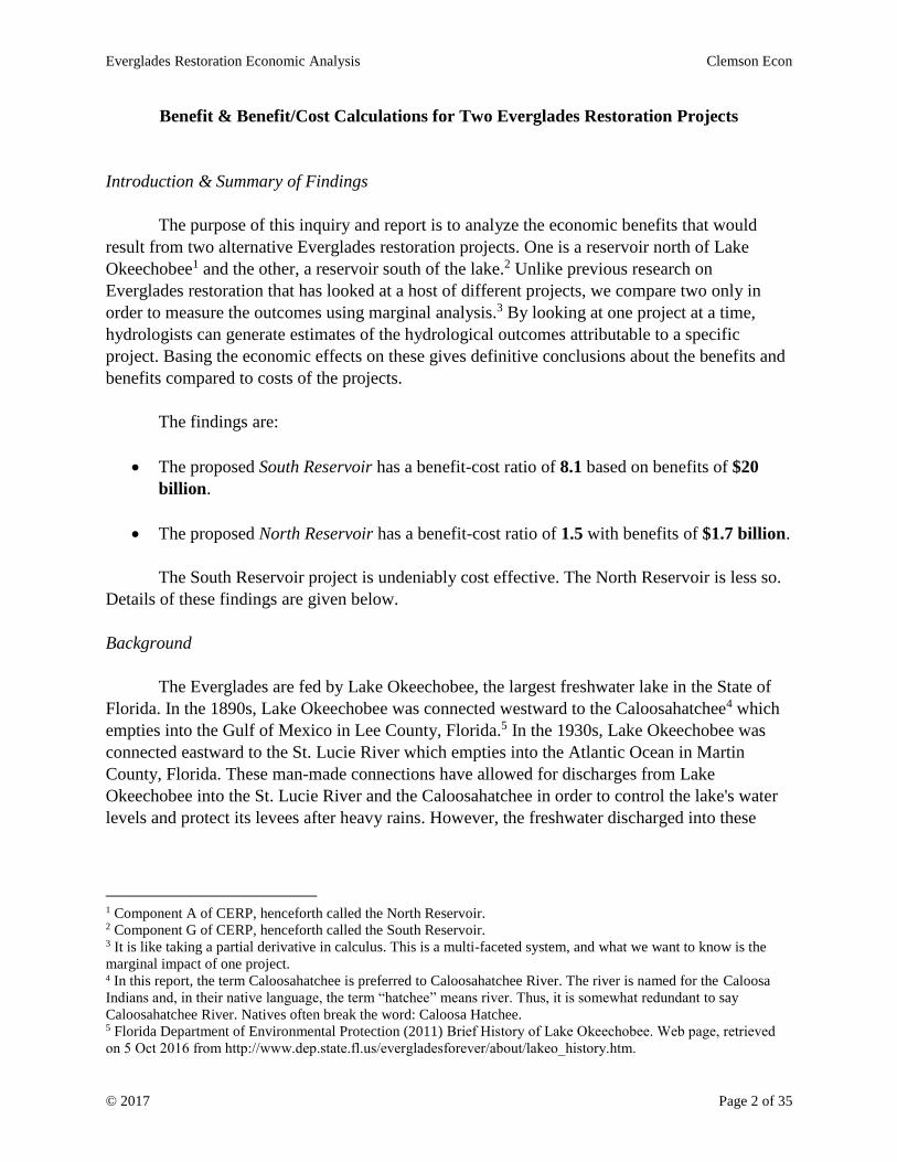
Abstract:
We calculate economic benefits from two alternative Everglades restoration projects. We call one
the South Reservoir, a reservoir south of Lake Okeechobee that would provide storage when the lake is
too full. The other is called the North Reservoir, a storage area north of Lake Okeechobee that will
capture water before it enters the lake. One purpose of the reservoirs is to mitigate the discharge of the
excess water from Lake Okeechobee into the St. Lucie River and the Caloosahatchee where it damages
the estuaries and negatively affects water quality. By investigating the effects of one reservoir at a time,
hydrologists can estimate the reduction in discharges into the rivers attributable to a specific project.
Prior research clearly shows that reducing discharges improves water quality. Research also
shows that improving water quality increases property values. We put these two pieces of scientific
evidence together to calculate the expected economic benefits of the South Reservoir and of the North
Reservoir compared to doing nothing.
The findings are dramatic. The South Reservoir outperforms the alternative of a North Reservoir,
improving water quality by more than 45% in the Caloosahatchee and 64% in the St. Lucie River. This
will cause property values of homes on or near the waterfront to increase by 18%, resulting in over $12
billion in increased value. Properties related to and serving those homes are also expected to increase in
value, adding about $6.5 billion in value. There’s also value in the water to be collected in the reservoir
that would otherwise be dumped into the seas. Adding this to the increased real estate value, the benefits
of the South Reservoir are expected to be over $20 billion. The cost of the South Reservoir is estimated to
be about $2.5 billion, so the net benefits are over $17 billion with a benefit-cost ratio of 8.1.
The North Reservoir is not nearly so effective at reducing discharges to the estuaries, and, hence,
will have economically less effect. It will only result in discharge mitigation of 5-6%. Benefits, counting
the value of the water, would be $1.7 billion with a benefits-cost ratio of 1.5.
From a hydrological perspective, the South Reservoir is clearly a superior project and our
economic analysis puts a dollar value on it that is conspicuously large. The beauty of doing a simple
simulation of one project at a time is that we get a clear picture of the outcome. The hydrology is basic
and the predicted economic outcome is definitive.
© 2017. This study has been funded by the Congressional Office of (retired) Representative Curt Clawson and by
the Everglades Foundation, but the Clemson University investigators are solely responsible for the content of the
report. Thomas is Visiting Assistant Professor, De Los Santos is Assistant Professor, Sauer and Parker are Masters
Students all in the Department of Economics, Clemson University. Hobbs (BS Clemson) is an industrial engineer at
Perkins + Will in Atlanta. This project is the outgrowth of work done previously by researchers at and associated
with Clemson University.
Everglades Restoration Economic Analysis Clemson Econ
© 2017 Page 2 of 35
Benefit & Benefit/Cost Calculations for Two Everglades Restoration Projects
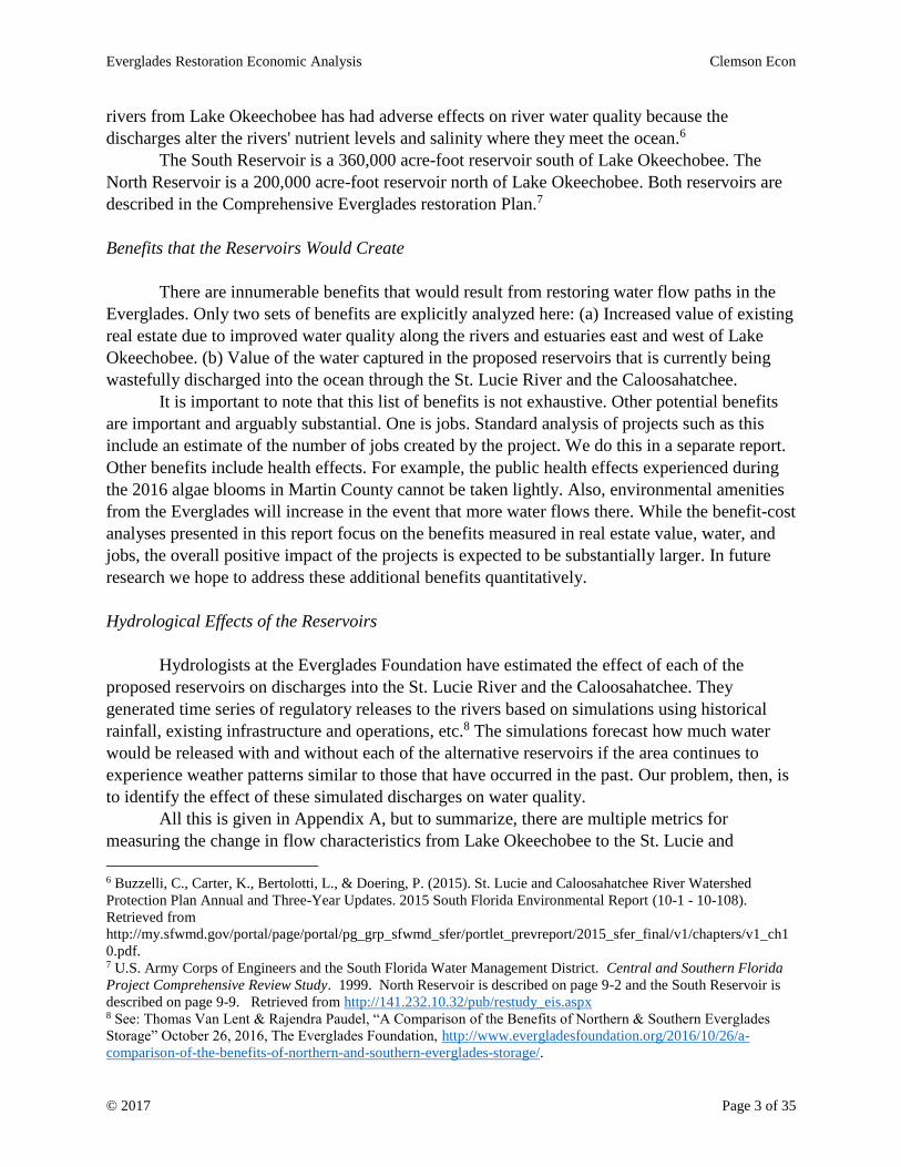
Introduction & Summary of Findings
The purpose of this inquiry and report is to analyze the economic benefits that would
result from two alternative Everglades restoration projects. One is a reservoir north of Lake
Okeechobee1 and the other, a reservoir south of the lake.2 Unlike previous research on
Everglades restoration that has looked at a host of different projects, we compare two only in
order to measure the outcomes using marginal analysis.3 By looking at one project at a time,
hydrologists can generate estimates of the hydrological outcomes attributable to a specific
project. Basing the economic effects on these gives definitive conclusions about the benefits and
benefits compared to costs of the projects.
The findings are:
The proposed South Reservoir has a benefit-cost ratio of 8.1 based on benefits of $20
billion.
The proposed North Reservoir has a benefit-cost ratio of 1.5 with benefits of $1.7 billion.
The South Reservoir project is undeniably cost effective. The North Reservoir is less so.
Details of these findings are given below.
Background
The Everglades are fed by Lake Okeechobee, the largest freshwater lake in the State of
Florida. In the 1890s, Lake Okeechobee was connected westward to the Caloosahatchee4 which
empties into the Gulf of Mexico in Lee County, Florida.5 In the 1930s, Lake Okeechobee was
connected eastward to the St. Lucie River which empties into the Atlantic Ocean in Martin
County, Florida. These man-made connections have allowed for discharges from Lake
Okeechobee into the St. Lucie River and the Caloosahatchee in order to control the lake's water
levels and protect its levees after heavy rains. However, the freshwater discharged into these
1 Component A of CERP, henceforth called the North Reservoir. 2 Component G of CERP, henceforth called the South Reservoir. 3 It is like taking a partial derivative in calculus. This is a multi-faceted system, and what we want to know is the
marginal impact of one project. 4 In this report, the term Caloosahatchee is preferred to Caloosahatchee River. The river is named for the Caloosa
Indians and, in their native language, the term “hatchee” means river. Thus, it is somewhat redundant to say
Caloosahatchee River. Natives often break the word: Caloosa Hatchee. 5 Florida Department of Environmental Protection (2011) Brief History of Lake Okeechobee. Web page, retrieved
on 5 Oct 2016 from http://www.dep.state.fl.us/evergladesforever/about/lakeo_history.htm.
Everglades Restoration Economic Analysis Clemson Econ
© 2017 Page 3 of 35
rivers from Lake Okeechobee has had adverse effects on river water quality because the
discharges alter the rivers' nutrient levels and salinity where they meet the ocean.6
The South Reservoir is a 360,000 acre-foot reservoir south of Lake Okeechobee. The
North Reservoir is a 200,000 acre-foot reservoir north of Lake Okeechobee. Both reservoirs are
described in the Comprehensive Everglades restoration Plan.7
Benefits that the Reservoirs Would Create
There are innumerable benefits that would result from restoring water flow paths in the
Everglades. Only two sets of benefits are explicitly analyzed here: (a) Increased value of existing
real estate due to improved water quality along the rivers and estuaries east and west of Lake
Okeechobee. (b) Value of the water captured in the proposed reservoirs that is currently being
wastefully discharged into the ocean through the St. Lucie River and the Caloosahatchee.
It is important to note that this list of benefits is not exhaustive. Other potential benefits
are important and arguably substantial. One is jobs. Standard analysis of projects such as this
include an estimate of the number of jobs created by the project. We do this in a separate report.
Other benefits include health effects. For example, the public health effects experienced during
the 2016 algae blooms in Martin County cannot be taken lightly. Also, environmental amenities
from the Everglades will increase in the event that more water flows there. While the benefit-cost
analyses presented in this report focus on the benefits measured in real estate value, water, and
jobs, the overall positive impact of the projects is expected to be substantially larger. In future
research we hope to address these additional benefits quantitatively.
Hydrological Effects of the Reservoirs
Hydrologists at the Everglades Foundation have estimated the effect of each of the
proposed reservoirs on discharges into the St. Lucie River and the Caloosahatchee. They
generated time series of regulatory releases to the rivers based on simulations using historical
rainfall, existing infrastructure and operations, etc.8 The simulations forecast how much water
would be released with and without each of the alternative reservoirs if the area continues to
experience weather patterns similar to those that have occurred in the past. Our problem, then, is
to identify the effect of these simulated discharges on water quality.
All this is given in Appendix A, but to summarize, there are multiple metrics for
measuring the change in flow characteristics from Lake Okeechobee to the St. Lucie and
6 Buzzelli, C., Carter, K., Bertolotti, L., & Doering, P. (2015). St. Lucie and Caloosahatchee River Watershed
Protection Plan Annual and Three-Year Updates. 2015 South Florida Environmental Report (10-1 - 10-108).
Retrieved from
http://my.sfwmd.gov/portal/page/portal/pg_grp_sfwmd_sfer/portlet_prevreport/2015_sfer_final/v1/chapters/v1_ch1
0.pdf. 7 U.S. Army Corps of Engineers and the South Florida Water Management District. Central and Southern Florida
Project Comprehensive Review Study. 1999. North Reservoir is described on page 9-2 and the South Reservoir is
described on page 9-9. Retrieved from http://141.232.10.32/pub/restudy_eis.aspx 8 See: Thomas Van Lent & Rajendra Paudel, “A Comparison of the Benefits of Northern & Southern Everglades
Storage” October 26, 2016, The Everglades Foundation, http://www.evergladesfoundation.org/2016/10/26/a-
comparison-of-the-benefits-of-northern-and-southern-everglades-storage/.
Everglades Restoration Economic Analysis Clemson Econ
© 2017 Page 4 of 35
Caloosahatchee estuaries. Volume, duration, and frequency are all defining characteristics. To
maintain all of the characteristics, we use the modeled time series of monthly regulatory release
totals and link these monthly flow totals to water quality metrics. To get the relation between
monthly flows and water quality we use the relationships observed in past actual releases,
thereby generating a time series of water quality.
We choose Secchi disk depth (SDD) as our water quality metric. SDD is a measure of
water quality based on visual assessment of clarity. SDD has proven to be the most robust link
between consumers’ market-value expression of their appreciation of water quality and the
water’s underlying composition. That is, SDD is the metric of water quality most highly
correlated with the market value of residential property.
We know from the hydrological literature that SDD responds negatively to pollution
load. Specifically, as the phosphorus content of the water decreases, SDD goes up. We also
know that discharges from Lake Okeechobee have high phosphorus content. To map these
discharges into SDD we run regressions of SDD readings on the observed releases. The
regressions show the predicted negative relation and are statistically significant.
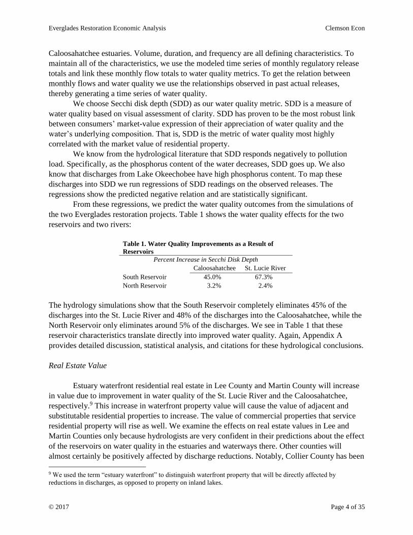
From these regressions, we predict the water quality outcomes from the simulations of
the two Everglades restoration projects. Table 1 shows the water quality effects for the two
reservoirs and two rivers:
Table 1. Water Quality Improvements as a Result of
Reservoirs
Percent Increase in Secchi Disk Depth
Caloosahatchee St. Lucie River
South Reservoir 45.0% 67.3%
North Reservoir 3.2% 2.4%
The hydrology simulations show that the South Reservoir completely eliminates 45% of the
discharges into the St. Lucie River and 48% of the discharges into the Caloosahatchee, while the
North Reservoir only eliminates around 5% of the discharges. We see in Table 1 that these
reservoir characteristics translate directly into improved water quality. Again, Appendix A
provides detailed discussion, statistical analysis, and citations for these hydrological conclusions.
Real Estate Value
Estuary waterfront residential real estate in Lee County and Martin County will increase
in value due to improvement in water quality of the St. Lucie River and the Caloosahatchee,
respectively.9 This increase in waterfront property value will cause the value of adjacent and
substitutable residential properties to increase. The value of commercial properties that service
residential property will rise as well. We examine the effects on real estate values in Lee and
Martin Counties only because hydrologists are very confident in their predictions about the effect
of the reservoirs on water quality in the estuaries and waterways there. Other counties will
almost certainly be positively affected by discharge reductions. Notably, Collier County has been
9 We used the term “estuary waterfront” to distinguish waterfront property that will be directly affected by
reductions in discharges, as opposed to property on inland lakes.
Everglades Restoration Economic Analysis Clemson Econ
© 2017 Page 5 of 35
plagued by algae blooms attributed to Caloosahatchee discharges. Nonetheless, hydrologists
cannot be precise about the degree to which reduced discharges will translate into higher water
quality there. In future work we may be able measure benefits beyond Lee and Martin Counties.
Many researchers have estimated the impact of improved water quality on waterfront and
adjacent properties. Florida Realtors® conducted an exhaustive study controlling for almost all
factors that affect residential property values.10 Their statistical analysis finds that home values
are positively affected by proximity to water and the quality of that water; that is, the closer a
home is to water and the higher the quality of that water, the higher its value holding everything
else constant. Florida Realtors use an exponential decay function to best fit the relation between
distance from the water and the relative impact of water and water quality on the price of the
property. The function quantifies how the relative amenity value of proximity to the water and its
quality declines as distance from the water increases. We apply this model to measure the
increase in real estate value from improved water quality caused by the North and South
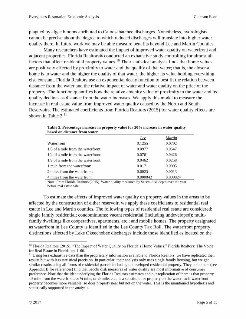
Reservoirs. The estimated coefficients from Florida Realtors (2015) for water quality effects are
shown in Table 2.11
Table 2. Percentage increase in property value for 20% increase in water quality
based on distance from water
Lee Martin
Waterfront 0.1255 0.0702
1/8 of a mile from the waterfront: 0.0977 0.0547
1/4 of a mile from the waterfront: 0.0761 0.0426
1/2 of a mile from the waterfront: 0.0462 0.0258
1 mile from the waterfront: 0.017 0.0095
2 miles from the waterfront: 0.0023 0.0013
4 miles from the waterfront: 0.000042 0.000024 Note: From Florida Realtors (2015). Water quality measured by Secchi disk depth over the year
before real estate sale.
To estimate the effects of improved water quality on property values in the areas to be
affected by the construction of either reservoir, we apply these coefficients to residential real
estate in Lee and Martin counties. The following types of residential real estate are considered:
single family residential; condominiums; vacant residential (including undeveloped); multi-
family dwellings like cooperatives, apartments, etc.; and mobile homes. The property designated
as waterfront in Lee County is identified in the Lee County Tax Roll. The waterfront property
distinctions affected by Lake Okeechobee discharges include those identified as located on the
10 Florida Realtors (2015), “The Impact of Water Quality on Florida’s Home Values,” Florida Realtors: The Voice
for Real Estate in Florida pp. 1-60. 11 Using less exhaustive data than the proprietary information available to Florida Realtors, we have replicated their
results but with less statistical precision. In particular, their analysis only uses single family housing, but we get
similar results using all forms of residential parcels including undeveloped residential property. They and others (see
Appendix B for references) find that Secchi disk measures of water quality are most informative of consumer
preference. Note that the idea underlying the Florida Realtors estimates and our replication of them is that property
1/8 mile from the waterfront, or ¼ mile, or ½ mile, etc., is a substitute for property on the water, so if waterfront
property becomes more valuable, so does property near but not on the water. This is the maintained hypothesis and
statistically supported in the analysis.
Everglades Restoration Economic Analysis Clemson Econ
© 2017 Page 6 of 35
Gulf, Bay, Canal, River, or Creek.12 The property designated as waterfront in Martin County is
identified in the Martin County Tax Roll. The waterfront property distinctions affected by Lake
Okeechobee discharges are listed in Table C1. Geographic information system (GIS) maps
available through each county’s property appraiser were used to measure distance from
waterfront property to adjacent properties. The valuations used are the preliminary property tax
rolls for 2016 for Lee and Martin Counties as of July 2016. Individual parcel value for each
property in each county was measured by the appraiser’s just value.13 14
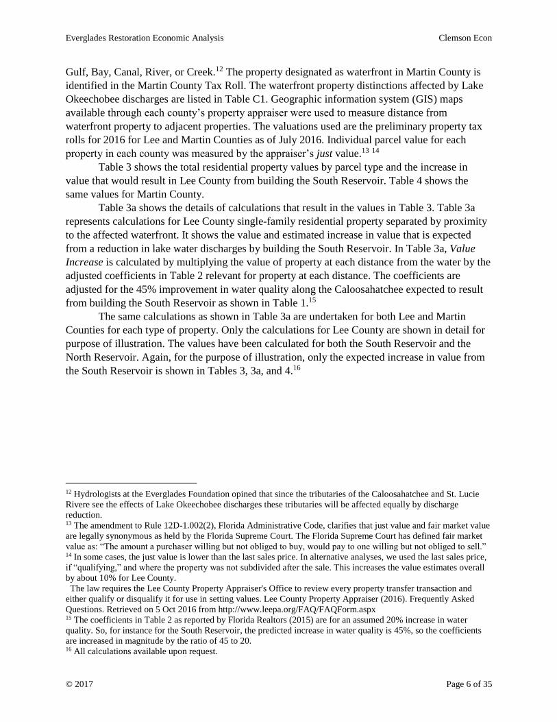
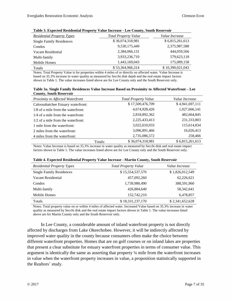
Table 3 shows the total residential property values by parcel type and the increase in
value that would result in Lee County from building the South Reservoir. Table 4 shows the
same values for Martin County.
Table 3a shows the details of calculations that result in the values in Table 3. Table 3a
represents calculations for Lee County single-family residential property separated by proximity
to the affected waterfront. It shows the value and estimated increase in value that is expected
from a reduction in lake water discharges by building the South Reservoir. In Table 3a, Value
Increase is calculated by multiplying the value of property at each distance from the water by the
adjusted coefficients in Table 2 relevant for property at each distance. The coefficients are
adjusted for the 45% improvement in water quality along the Caloosahatchee expected to result
from building the South Reservoir as shown in Table 1.15
The same calculations as shown in Table 3a are undertaken for both Lee and Martin
Counties for each type of property. Only the calculations for Lee County are shown in detail for
purpose of illustration. The values have been calculated for both the South Reservoir and the
North Reservoir. Again, for the purpose of illustration, only the expected increase in value from
the South Reservoir is shown in Tables 3, 3a, and 4.16
12 Hydrologists at the Everglades Foundation opined that since the tributaries of the Caloosahatchee and St. Lucie
Rivere see the effects of Lake Okeechobee discharges these tributaries will be affected equally by discharge
reduction. 13 The amendment to Rule 12D-1.002(2), Florida Administrative Code, clarifies that just value and fair market value
are legally synonymous as held by the Florida Supreme Court. The Florida Supreme Court has defined fair market
value as: “The amount a purchaser willing but not obliged to buy, would pay to one willing but not obliged to sell.” 14 In some cases, the just value is lower than the last sales price. In alternative analyses, we used the last sales price,
if “qualifying,” and where the property was not subdivided after the sale. This increases the value estimates overall
by about 10% for Lee County.
The law requires the Lee County Property Appraiser's Office to review every property transfer transaction and
either qualify or disqualify it for use in setting values. Lee County Property Appraiser (2016). Frequently Asked
Questions. Retrieved on 5 Oct 2016 from http://www.leepa.org/FAQ/FAQForm.aspx 15 The coefficients in Table 2 as reported by Florida Realtors (2015) are for an assumed 20% increase in water
quality. So, for instance for the South Reservoir, the predicted increase in water quality is 45%, so the coefficients
are increased in magnitude by the ratio of 45 to 20. 16 All calculations available upon request.
Everglades Restoration Economic Analysis Clemson Econ
© 2017 Page 7 of 35
Table 3. Expected Residential Property Value Increase - Lee County, South Reservoir
Residential Property Types Total Property Value Value Increase
Single Family Residences $ 36,074,318,981 $ 6,815,261,613
Condos 9,530,175,449 2,375,987,588
Vacant Residential 2,384,066,131 444,059,566
Multi-family 3,933,236,710 579,623,118
Mobile Homes 1,443,169,043 175,089,158
Totals $ 53,364,966,314 $ 10,390,021,043 Notes: Total Property Value is for properties within 4 miles of or directly on affected water. Value Increase is
based on 35.3% increase in water quality as measured by Secchi disk depth and the real estate impact factors
shown in Table 1. The value increases listed above are for Lee County only and the South Reservoir only.
Table 3a. Single Family Residences Value Increase Based on Proximity to Affected Waterfront – Lee
County, South Reservoir
Proximity to Affected Waterfront Total Property Value Value Increase
Caloosahatchee Estuary waterfront: $ 17,500,476,709 $ 4,941,697,111
1/8 of a mile from the waterfront: 4,674,928,426 1,027,666,141
1/4 of a mile from the waterfront: 2,818,892,362 482,664,845
1/2 of a mile from the waterfront: 2,225,433,413 231,333,803
1 mile from the waterfront: 3,022,610,033 115,614,834
2 miles from the waterfront: 3,096,891,466 16,026,413
4 miles from the waterfront: 2,735,086,572 258,466
Totals: $ 36,074,318,981 $ 6,815,261,613 Notes: Value Increase is based on 35.3% increase in water quality as measured by Secchi disk and real estate impact
factors shown in Table 1. The value increases listed above are for Lee County only and the South Reservoir only.
Table 4. Expected Residential Property Value Increase - Martin County, South Reservoir
Residential Property Types Total Property Value Value Increase
Single Family Residences $ 15,554,537,570 $ 1,826,012,549
Vacant Residential 457,092,260 62,226,621
Condos 1,739,980,490 388,591,960
Multi-family 426,884,640 58,342,641
Mobile Homes 152,742,210 6,478,857
Totals $ 18,331,237,170 $ 2,341,652,628
Notes: Total property value on or within 4 miles of affected water. Increased Value based on 35.3% increase in water
quality as measured by Secchi disk and the real estate impact factors shown in Table 1. The value increases listed
above are for Martin County only and the South Reservoir only.
In Lee County, a considerable amount of inland waterfront property is not directly
affected by discharges from Lake Okeechobee. However, it will be indirectly affected by
improved water quality in the county because consumers often make the choice between
different waterfront properties. Homes that are on golf courses or on inland lakes are properties
that present a clear substitute for estuary waterfront properties in terms of consumer value. This
argument is identically the same as asserting that property ¼ mile from the waterfront increases
in value when the waterfront property increases in value, a proposition statistically supported in
the Realtors’ study.
Everglades Restoration Economic Analysis Clemson Econ
© 2017 Page 8 of 35
To account for the relation in value between golf course and inland lake properties and
the properties directly affected by discharges from Lake Okeechobee, a time-series regression
model for sales data over the last 40 years is used. The full analysis is presented in Appendix D.
The estimated relation factor between changes in value of these residential properties is 0.776.
That is, whenever estuary waterfront property has gone up by 10% in a year, golf course and lake
property has gone up by 7.76% in that year.
We did a similar analysis for commercial property such as supermarkets and shopping
centers. This estimated relation factor is 0.655. That is, whenever estuary waterfront property has
gone up 10% in a year, commercial property that can reasonably be expected to serve residential
consumers has gone up 6.55% in that year.
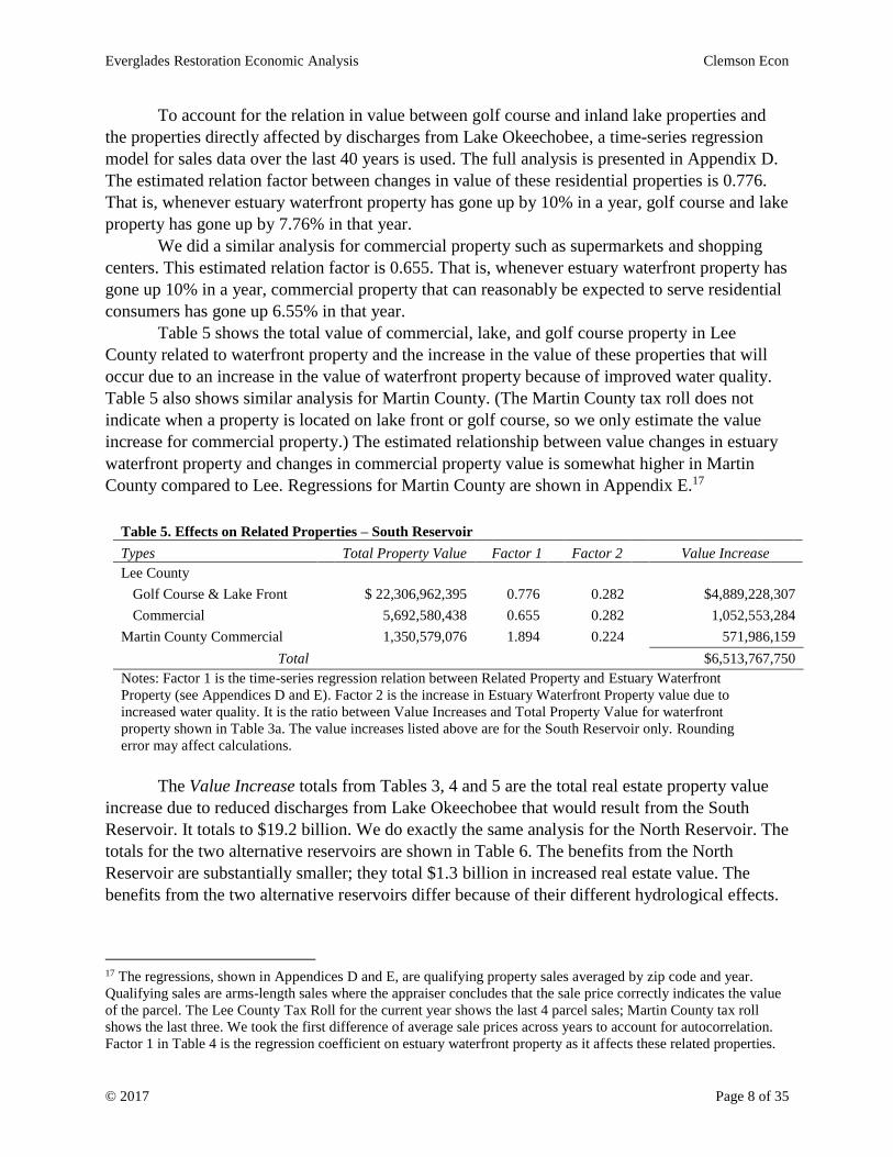
Table 5 shows the total value of commercial, lake, and golf course property in Lee
County related to waterfront property and the increase in the value of these properties that will
occur due to an increase in the value of waterfront property because of improved water quality.
Table 5 also shows similar analysis for Martin County. (The Martin County tax roll does not
indicate when a property is located on lake front or golf course, so we only estimate the value
increase for commercial property.) The estimated relationship between value changes in estuary
waterfront property and changes in commercial property value is somewhat higher in Martin
County compared to Lee. Regressions for Martin County are shown in Appendix E.17
Table 5. Effects on Related Properties – South Reservoir
Types Total Property Value Factor 1 Factor 2 Value Increase Lee County
Golf Course & Lake Front $ 22,306,962,395 0.776 0.282 $4,889,228,307 Commercial 5,692,580,438 0.655 0.282 1,052,553,284
Martin County Commercial 1,350,579,076 1.894 0.224 571,986,159
Total $6,513,767,750 Notes: Factor 1 is the time-series regression relation between Related Property and Estuary Waterfront
Property (see Appendices D and E). Factor 2 is the increase in Estuary Waterfront Property value due to
increased water quality. It is the ratio between Value Increases and Total Property Value for waterfront
property shown in Table 3a. The value increases listed above are for the South Reservoir only. Rounding
error may affect calculations.
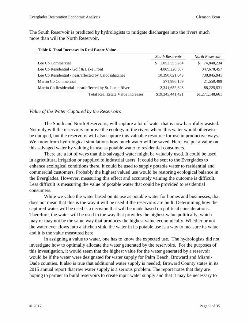
The Value Increase totals from Tables 3, 4 and 5 are the total real estate property value
increase due to reduced discharges from Lake Okeechobee that would result from the South
Reservoir. It totals to $19.2 billion. We do exactly the same analysis for the North Reservoir. The
totals for the two alternative reservoirs are shown in Table 6. The benefits from the North
Reservoir are substantially smaller; they total $1.3 billion in increased real estate value. The
benefits from the two alternative reservoirs differ because of their different hydrological effects.
17 The regressions, shown in Appendices D and E, are qualifying property sales averaged by zip code and year.
Qualifying sales are arms-length sales where the appraiser concludes that the sale price correctly indicates the value
of the parcel. The Lee County Tax Roll for the current year shows the last 4 parcel sales; Martin County tax roll
shows the last three. We took the first difference of average sale prices across years to account for autocorrelation.
Factor 1 in Table 4 is the regression coefficient on estuary waterfront property as it affects these related properties.
Everglades Restoration Economic Analysis Clemson Econ
© 2017 Page 9 of 35
The South Reservoir is predicted by hydrologists to mitigate discharges into the rivers much
more than will the North Reservoir.
Table 6. Total Increases in Real Estate Value
South Reservoir North Reservoir
Lee Co Commercial $ 1,052,553,284 $ 74,848,234
Lee Co Residential - Golf & Lake Front 4,889,228,307 347,678,457
Lee Co Residential - near/affected by Caloosahatchee 10,390,021,043 738,845,941
Martin Co Commercial 571,986,159 21,550,499
Martin Co Residential - near/affected by St. Lucie River 2,341,652,628 88,225,531
Total Real Estate Value Increases $19,245,441,421 $1,271,148,661
Value of the Water Captured by the Reservoirs
The South and North Reservoirs, will capture a lot of water that is now harmfully wasted.
Not only will the reservoirs improve the ecology of the rivers where this water would otherwise
be dumped, but the reservoirs will also capture this valuable resource for use in productive ways.
We know from hydrological simulations how much water will be saved. Here, we put a value on
this salvaged water by valuing its use as potable water to residential consumers.
There are a lot of ways that this salvaged water might be valuably used. It could be used
in agricultural irrigation or supplied to industrial users. It could be sent to the Everglades to
enhance ecological conditions there. It could be used to supply potable water to residential and
commercial customers. Probably the highest valued use would be restoring ecological balance in
the Everglades. However, measuring this effect and accurately valuing the outcome is difficult.
Less difficult is measuring the value of potable water that could be provided to residential
consumers.
While we value the water based on its use as potable water for homes and businesses, that
does not mean that this is the way it will be used if the reservoirs are built. Determining how the
captured water will be used is a decision that will be made based on political considerations.
Therefore, the water will be used in the way that provides the highest value politically, which
may or may not be the same way that produces the highest value economically. Whether or not
the water ever flows into a kitchen sink, the water in its potable use is a way to measure its value,
and it is the value measured here.
In assigning a value to water, one has to know the expected use. The hydrologists did not
investigate how to optimally allocate the water generated by the reservoirs. For the purposes of
this investigation, it would seem that the highest value for the water generated by a reservoir
would be if the water were designated for water supply for Palm Beach, Broward and Miami-
Dade counties. It also is true that additional water supply is needed; Broward County states in its
2015 annual report that raw water supply is a serious problem. The report notes that they are
hoping to partner to build reservoirs to create input water supply and that it may be necessary to
Everglades Restoration Economic Analysis Clemson Econ
© 2017 Page 10 of 35
tap into brackish ground water that will require desalination. 18 Moreover, as the water could be
allocated using the existing infrastructure and the decision on water allocation belongs to the
state of Florida, the water in these reservoirs is theoretically available for water supply. Based
on this, we conclude that desalination of brackish groundwater is the opportunity cost of the
water supply that can be created by the South and North Reservoirs.
There are several ways to measure desalination cost. One method measures observed
desalination cost for existing plants in the U.S. and around the world. A second measures the
differential costs between water systems in Florida that do and do not face brackish groundwater.
The first method gives an estimate of $2 per 1000 gallons [$/kgal]. The second, $1.43/kgal.
Details of these estimates are given in Appendix F.
To tally up the benefits of the water captured by the reservoirs we need to know how
much water would be made available for potable purposes. Again, the function of the reservoirs
is to take water out of Lake Okeechobee (or preventing water from reaching it) when the lake is
excessively high and instead of dumping it into the rivers, holding it until it becomes valuable.
Hydrologists model flows into the reservoirs and can estimate how much of this water would be
usefully transferred from wet times to dry times. The South Reservoir is estimated to generate
11,370,000 kgal per year on average. The North Reservoir is estimated to generate 6,253,000
kgal per year on average. These are gallons of water potentially available at the wellheads of
water districts. That is, these numbers are based on water released from the reservoirs into canals
that then could find its way into the aquifers that are tapped by potable water suppliers.
Note that the South Reservoir will also supply water into the Everglades and this will
have value. Environmentally beneficial water could occur in either a wet period or a dry period.
Since there is no current way to separate water delivered in wet periods and dry periods, we
simply recognize that it has value, but do not attempt to quantify. We hope to measure this in
future research.
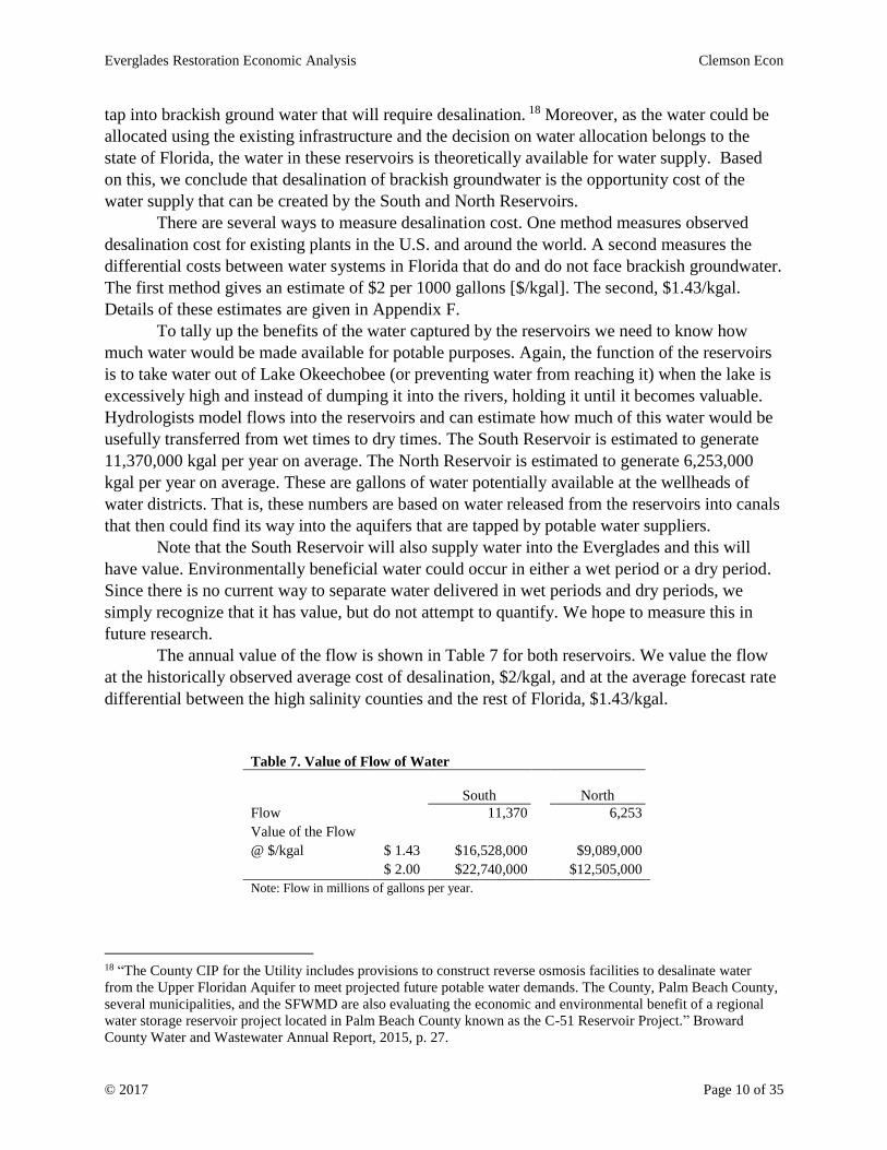
The annual value of the flow is shown in Table 7 for both reservoirs. We value the flow
at the historically observed average cost of desalination, $2/kgal, and at the average forecast rate
differential between the high salinity counties and the rest of Florida, $1.43/kgal.
Table 7. Value of Flow of Water
South
North
Flow 11,370 6,253
Value of the Flow
@ $/kgal $ 1.43 $16,528,000 $9,089,000
$ 2.00 $22,740,000 $12,505,000
Note: Flow in millions of gallons per year.
18 “The County CIP for the Utility includes provisions to construct reverse osmosis facilities to desalinate water
from the Upper Floridan Aquifer to meet projected future potable water demands. The County, Palm Beach County,
several municipalities, and the SFWMD are also evaluating the economic and environmental benefit of a regional
water storage reservoir project located in Palm Beach County known as the C-51 Reservoir Project.” Broward
County Water and Wastewater Annual Report, 2015, p. 27.
Everglades Restoration Economic Analysis Clemson Econ
© 2017 Page 11 of 35
The present discounted value [PDV] of this annual flow of benefits depends on the life of
the project and the discount rate. We set the life of the project at 50 years. It remains to choose
the discount rate.
We varied the discount rate used in our calculations to show the impact of different
choices.19 We use nominal rates of 1.66%, 2.625%, and 3.125%. Details of these alternative rates
are given in Appendix F. Based on a forecast inflation rate of 1.66%, which is derived from the
yield on inflation protected bonds, the nominal rates imply real discount rates of zero, 0.97%,
and 1.47%, respectively. Nominal discount rates include the expected inflation rate. The nominal
rate essentially says that a dollar next year is not worth as much as a dollar today because prices
will go up due to inflation. However, this means that the value of water will also go up. So if we
discount using the nominal rate, we have to increase the value of the water at the inflation rate as
well. A mathematically equivalent calculation is to subtract the inflation rate from the nominal
rate, call it the real rate, and use that for discounting.
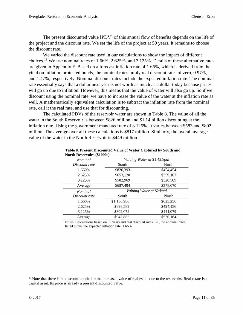
The calculated PDVs of the reservoir water are shown in Table 8. The value of all the
water in the South Reservoir is between $826 million and $1.14 billion discounting at the
inflation rate. Using the government mandated rate of 3.125%, it varies between $583 and $802
million. The average over all these calculations is $817 million. Similarly, the overall average
value of the water in the North Reservoir is $449 million.
Table 8. Present Discounted Value of Water Captured by South and
North Reservoirs ($1000s)
Nominal Valuing Water at $1.43/kgal
Discount rate South North
1.660% $826,393 $454,454
2.625% $653,120 $359,167
3.125% $582,969 $320,589
Average $687,494 $378,070
Nominal Valuing Water at $2/kgal
Discount rate South North
1.660% $1,136,986 $625,256
2.625% $898,589 $494,156
3.125% $802,072 $441,079
Average $945,882 $520,164
Notes: Calculations based on 50 years and real discount rates, i.e., the nominal rates
listed minus the expected inflation rate, 1.66%.
19 Note that there is no discount applied to the increased value of real estate due to the reservoirs. Real estate is a
capital asset. Its price is already a present discounted value.
Everglades Restoration Economic Analysis Clemson Econ
© 2017 Page 12 of 35
Costs
The South Reservoir is estimated to cost approximately $2.47 billion. This cost was
estimated by engineers using the same methodology employed by the U.S. Army Corps of
Engineers. The total estimated cost includes land cost and other expenses related to building the
reservoir, such as infrastructure development. The total cost per acre-foot is estimated at
$6,869.79, and applying this cost to the proposed acre-footage of 360,000 acre-feet results in the
estimated costs of $2.47 billion.20
The cost of the North Reservoir is taken from six projects analyzed by the U.S. Army
Corps of Engineers and the South Florida Water Management District.21 These projects range in
size from 155,000 to 321,000 acre feet, with costs proportionally ranging from $896,000 to
$1,802,000. Thus, a 200,000 acre-foot reservoir is estimated from these alternative projects to be
$1.1 billion.22
Benefits Compared to Costs
Now we compare the increased real estate value and the value of the water to the cost of
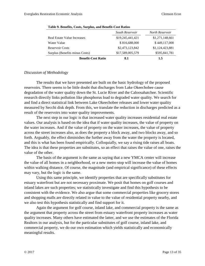
building the reservoirs. This is shown in Table 9. The cost of building the South Reservoir is
estimated to be $2.47 billion and is estimated to generate $20 billion in benefits comprised of
increased real estate value of $19 billion and water value of $817 million. This says that there
would be a surplus of $17.6 billion from building the South Reservoir. This surplus is commonly
characterized by the ratio of the benefits to costs. The benefit-cost ratio for the South Reservoir
is 8.1.23
The benefit-cost ratio for the North Reservoir is substantially smaller; it is 1.5. Benefits
are estimated to be greater than the costs by $596 million.
20 See: Thomas Van Lent & Rajendra Paudel, “A Comparison of the Benefits of Northern & Southern Everglades
Storage” October 26, 2016, The Everglades Foundation, http://www.evergladesfoundation.org/2016/10/26/a-
comparison-of-the-benefits-of-northern-and-southern-everglades-storage/; and Ardeshir Tehrani & Emmanuel Cruz,
“Preliminary Engineering Report Design and Cost Analysis of the Comprehensive Everglades restoration Plan
Southern Reservoir,” Prepared for: The Everglades Foundation, July 2016. 21 U.S. Army Corps of Engineers and South Florida Water Management District, "Lake Okeechobee Watershed
Restoration, Initial Array of Alternatives Overview" October 25, 2016. No supplemental information on how these
costs were developed is available. 22 These estimates do not include the cost of land, as the South Florida Water Management District states they
intended to construct on publicly-owned lands. However, in the Corps’ cost estimation, even publicly-owned lands
would have to be included in the cost. 23 Note that if land cost for the South Reservoir were to double, the benefit/cost ratio would still be 6.7 with a
surplus value of $17 billion.
Everglades Restoration Economic Analysis Clemson Econ
© 2017 Page 13 of 35
Table 9. Benefits, Costs, Surplus, and Benefit-Cost Ratios
South Reservoir North Reservoir
Real Estate Value Increases $19,245,441,421 $1,271,148,661
Water Value $ 816,688,000 $ 449,117,000
Reservoir Costs $2,473,123,842 $1,124,423,881
Surplus (Benefits minus Costs) $17,589,005,579 $595,841,781
Benefit-Cost Ratio 8.1 1.5
Discussion of Methodology
The results that we have presented are built on the basic hydrology of the proposed
reservoirs. There seems to be little doubt that discharges from Lake Okeechobee cause
degradation of the water quality down the St. Lucie River and the Caloosahatchee. Scientific
research directly links pollution like phosphorus load to degraded water quality. We search for
and find a direct statistical link between Lake Okeechobee releases and lower water quality
measured by Secchi disk depth. From this, we translate the reduction in discharges predicted as a
result of the reservoirs into water quality improvements.
The next step in our logic is that increased water quality increases residential real estate
values. Our analysis is based on the idea that if water quality increases, the value of property on
the water increases. And if the value of property on the water increases, the value of property
across the street increases also, as does the property a block away, and two blocks away, and so
forth. Arguably, the effect diminishes the further away from the water the property is located,
and this is what has been found empirically. Colloquially, we say a rising tide raises all boats.
The idea is that these properties are substitutes, so an effect that raises the value of one, raises the
value of the other.
The basis of the argument is the same as saying that a new YMCA center will increase
the value of all homes in a neighborhood, or a new metro stop will increase the value of homes
within walking distance. Of course, the magnitude (and empirical significance) of these effects
may vary, but the logic is the same.
Using this same principle, we identify properties that are specifically substitutes for
estuary waterfront but are not necessary proximate. We posit that homes on golf courses and
inland lakes are such properties; we statistically investigate and find this hypothesis to be
consistent with the evidence. We also argue that some commercial properties like grocery stores
and shopping malls are directly related in value to the value of residential property nearby, and
we also test this hypothesis statistically and find support for it.
Again the argument for golf course, inland lake, and commercial property is the same as
the argument that property across the street from estuary waterfront property increases as water
quality increases. Many others have estimated the latter, and we use the estimates of the Florida
Realtors in our analysis, but for the particular substitutes of golf course, inland lake, and
commercial property, we do our own estimation which yields statistically and economically
meaningful results.
Everglades Restoration Economic Analysis Clemson Econ
© 2017 Page 14 of 35
To forecast increases in real estate values, we use percentage changes. We express
improved water quality in percentage terms in Table 1. The Florida Realtors analysis is
expressed in percentage changes in Table 2. We multiply these factors and then multiply the
resulting product by current property values. This gives the dollar increase in waterfront and near
waterfront property value increases.
Summary of Findings
The proposed South Reservoir has an overall benefit-cost ratio of 8.1.
The total benefits are $19.25 billion in the increased value of real estate due to improved
water quality along the Caloosahatchee and St. Lucie River, and $817 million in the
value of the water collected in the reservoir.
The proposed North Reservoir has a benefit-cost ratio of 1.5.
The total benefits are $1.27 billion in the increased value of real estate due to improved
water quality and $449 million in the value of the water collected in the reservoir.
Conclusions
These benefit-cost findings speak loudly. The South Reservoir is clearly a project with
benefits vastly outweighing costs. The total benefits are estimated to be over $20 billion. At a
construction cost of $2.47 billion, the South Reservoir is a no-brainer.
We speak so strongly because the fundamental structure of the analysis is sound.
Nutrient-laden water that builds up in Lake Okeechobee is currently being dumped down rivers
into the Atlantic Ocean and Gulf of Mexico causing algae blooms that ruin water quality as well
as create malodorous effects for residents. Hard evidence has been amassed that people are
willing to pay for clean water and less stink where they live. Hydrological studies and our own
estimates show how much cleaner the water will be if excess water from Lake Okeechobee is not
dumped down the rivers to the seas. Simple, straightforward, and technically sound calculations
say the South Reservoir will increase the value of existing real estate in Lee and Martin Counties
by more than $19 billion, not to mention the value of the water that is currently, harmfully
wasted.
On the other hand, the North Reservoir is not as good of an investment economically
speaking. Based on our estimates, the benefit-cost ratio is greater than one but cost increases
(such as including land costs) could easily flip this. And, at all events, the North Reservoir's
benefits pale in comparison to the South Reservoir. The hydrologic modeling of the North
Reservoir shows that it eliminates Lake Okeechobee regulatory releases far less often than the
South Reservoir.24 The North Reservoir also captures less water. Hence, comparing the two
proposed projects on a cost-benefit basis, the South Reservoir project dominates.
24 See Table A2, Zero Flow.
Everglades Restoration Economic Analysis Clemson Econ
© 2017 Page 15 of 35
Comparing the benefit-cost ratio of South Reservoir to that of the North Reservoir is
simple and direct, as the numbers show. The longer the project is put off, the more it will cost to
build. We conclude the best option is to build the South Reservoir, and the sooner the better.
Appendix A:
The Effect of Water Discharges from Lake Okeechobee on Secchi
Disk Depth Measures of Water Quality
Our empirical analysis of how water quality affects the value of Florida real estate uses
Secchi disk depth (SDD) as the measure of water quality. SDD has proven to be the most robust
link between consumers’ appreciation of water quality and the water’s underlying composition.
(See Appendix B below.)
Hydrologists at the Everglades Foundation have provided us with predictions about how
each proposed reservoir will affect water discharges into the Caloosahatchee and the St. Lucie
River, relative to a baseline in which neither reservoir is built.25 To assess each reservoir’s
impact on real estate values, we therefore must translate the predicted changes in discharges into
predicted changes in SDD.
The relationship between water quality and discharges from the baseline revolves around
the causal relationship between total phosphorus (TP) and chlorophyll (Chl) in the waterway, and
the effects of these two on SDD. In an early examination of these underlying factors, Carlson
(1977) estimates the following relationships:
ln SDD = 2.04 – 0.68 ln Chl (equation 5, p. 364)
ln Chl = 1.449 ln TP – 2.442 (equation 7, p. 365)
ln SDD = 3.876 – 0.98 ln TP (equation 9, p. 365)
The final equation indicates that SDD varies almost one-to-one with the water’s
phosphorus content. For example, a 10% reduction in total phosphorus corresponds to a 9.8%
increase in SDD.
Carlson analyzed lakes. Concern that lakes differ from rivers and estuaries prompted
similar research on other types of waterways. Hoyer, et al. (2002) compare the relationship
between phosphorus and water quality measured by SDD in nearshore coastal waters on the west
coast of the Florida peninsula.26 Hence, their scientific analysis addresses precisely the issues
and locale with which we are concerned.
25 See: Thomas Van Lent & Rajendra Paudel, “A Comparison of the Benefits of Northern & Southern Everglades
Storage” October 26, 2016, The Everglades Foundation, http://www.evergladesfoundation.org/2016/10/26/a-
comparison-of-the-benefits-of-northern-and-southern-everglades-storage/. 26 See also, Garn, Herbert S., Rovertson, Dale M., Rose, William, J., & Saad, David A. (2010). Hydrology, Water
Quality, and Response to Changes in Phosphorous Loading of Minocqua and Kawaguesaga Lakes, Oneida County,
Wisconsin, With Special Emphasis on Effects of Urbanization. U.S. Geological Survey & U.S. Department of the
Interior. Scientific Investigations Report 2010-5196.
Everglades Restoration Economic Analysis Clemson Econ
© 2017 Page 16 of 35
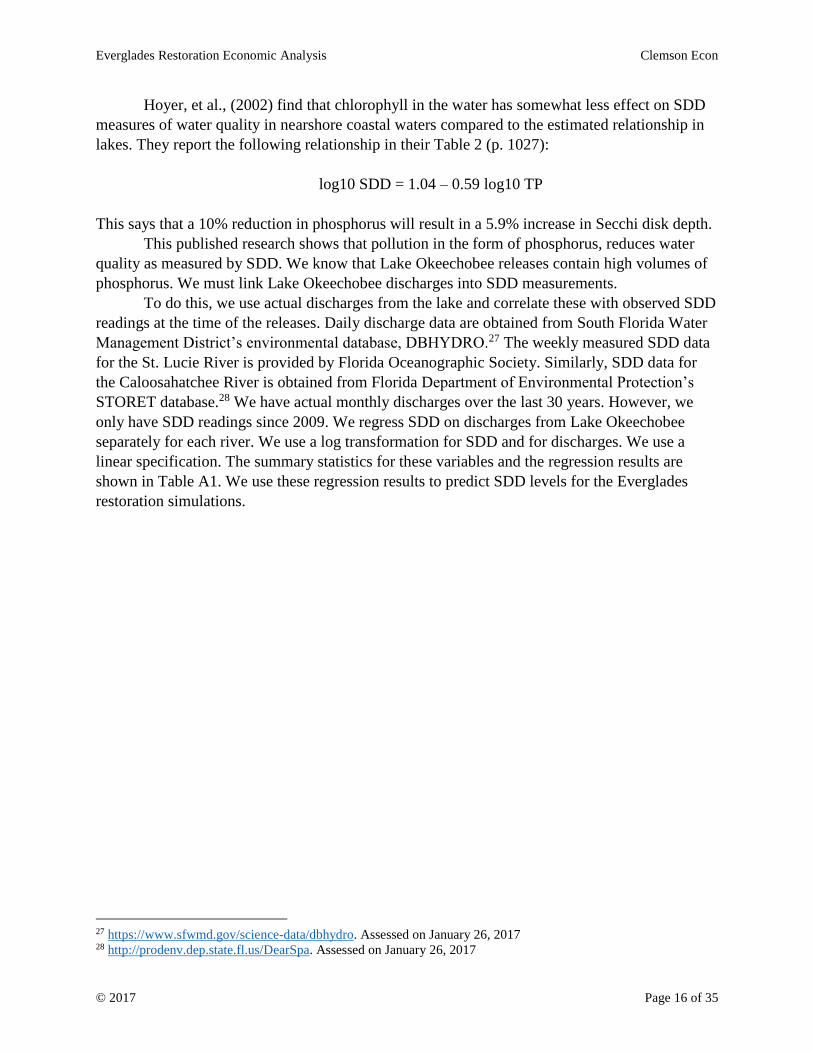
Hoyer, et al., (2002) find that chlorophyll in the water has somewhat less effect on SDD
measures of water quality in nearshore coastal waters compared to the estimated relationship in
lakes. They report the following relationship in their Table 2 (p. 1027):
log10 SDD = 1.04 – 0.59 log10 TP
This says that a 10% reduction in phosphorus will result in a 5.9% increase in Secchi disk depth.
This published research shows that pollution in the form of phosphorus, reduces water
quality as measured by SDD. We know that Lake Okeechobee releases contain high volumes of
phosphorus. We must link Lake Okeechobee discharges into SDD measurements.
To do this, we use actual discharges from the lake and correlate these with observed SDD
readings at the time of the releases. Daily discharge data are obtained from South Florida Water
Management District’s environmental database, DBHYDRO.27 The weekly measured SDD data
for the St. Lucie River is provided by Florida Oceanographic Society. Similarly, SDD data for
the Caloosahatchee River is obtained from Florida Department of Environmental Protection’s
STORET database.28 We have actual monthly discharges over the last 30 years. However, we
only have SDD readings since 2009. We regress SDD on discharges from Lake Okeechobee
separately for each river. We use a log transformation for SDD and for discharges. We use a
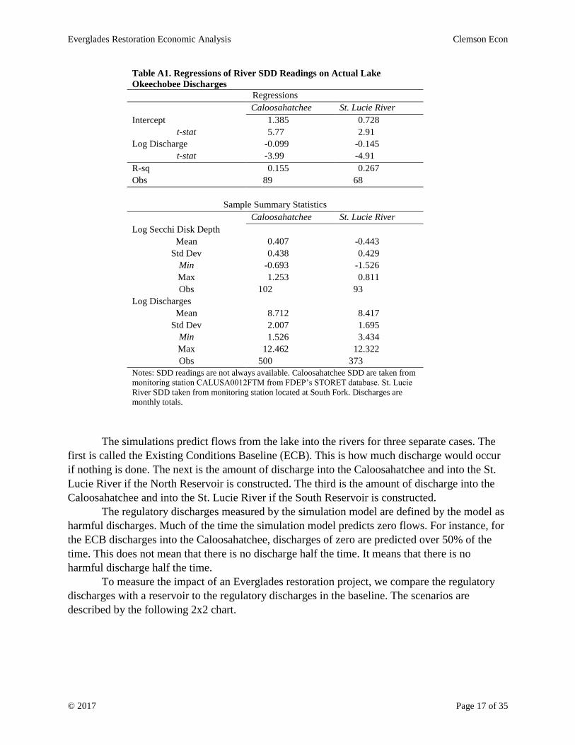
linear specification. The summary statistics for these variables and the regression results are
shown in Table A1. We use these regression results to predict SDD levels for the Everglades
restoration simulations.
27 https://www.sfwmd.gov/science-data/dbhydro. Assessed on January 26, 2017 28 http://prodenv.dep.state.fl.us/DearSpa. Assessed on January 26, 2017
Everglades Restoration Economic Analysis Clemson Econ
© 2017 Page 17 of 35
Table A1. Regressions of River SDD Readings on Actual Lake
Okeechobee Discharges
Regressions
Caloosahatchee St. Lucie River
Intercept 1.385 0.728
t-stat 5.77 2.91
Log Discharge -0.099 -0.145
t-stat -3.99 -4.91
R-sq 0.155 0.267
Obs 89 68
Sample Summary Statistics
Caloosahatchee St. Lucie River
Log Secchi Disk Depth
Mean 0.407 -0.443
Std Dev 0.438 0.429
Min -0.693 -1.526
Max 1.253 0.811
Obs 102 93
Log Discharges
Mean 8.712 8.417
Std Dev 2.007 1.695
Min 1.526 3.434
Max 12.462 12.322
Obs 500 373
Notes: SDD readings are not always available. Caloosahatchee SDD are taken from
monitoring station CALUSA0012FTM from FDEP’s STORET database. St. Lucie
River SDD taken from monitoring station located at South Fork. Discharges are
monthly totals.
The simulations predict flows from the lake into the rivers for three separate cases. The
first is called the Existing Conditions Baseline (ECB). This is how much discharge would occur
if nothing is done. The next is the amount of discharge into the Caloosahatchee and into the St.
Lucie River if the North Reservoir is constructed. The third is the amount of discharge into the
Caloosahatchee and into the St. Lucie River if the South Reservoir is constructed.
The regulatory discharges measured by the simulation model are defined by the model as
harmful discharges. Much of the time the simulation model predicts zero flows. For instance, for
the ECB discharges into the Caloosahatchee, discharges of zero are predicted over 50% of the
time. This does not mean that there is no discharge half the time. It means that there is no
harmful discharge half the time.
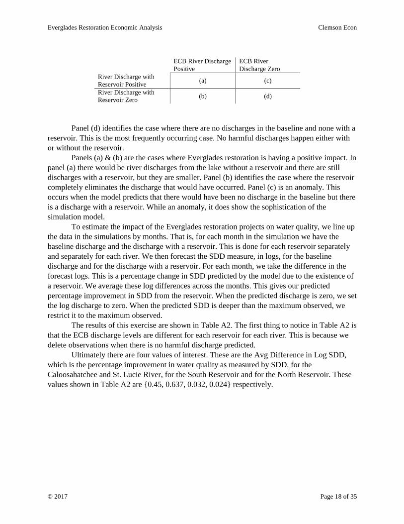
To measure the impact of an Everglades restoration project, we compare the regulatory
discharges with a reservoir to the regulatory discharges in the baseline. The scenarios are
described by the following 2x2 chart.
Everglades Restoration Economic Analysis Clemson Econ
© 2017 Page 18 of 35
ECB River Discharge
Positive
ECB River
Discharge Zero
River Discharge with
Reservoir Positive (a) (c)
River Discharge with
Reservoir Zero (b) (d)
Panel (d) identifies the case where there are no discharges in the baseline and none with a
reservoir. This is the most frequently occurring case. No harmful discharges happen either with
or without the reservoir.
Panels (a) & (b) are the cases where Everglades restoration is having a positive impact. In
panel (a) there would be river discharges from the lake without a reservoir and there are still
discharges with a reservoir, but they are smaller. Panel (b) identifies the case where the reservoir
completely eliminates the discharge that would have occurred. Panel (c) is an anomaly. This
occurs when the model predicts that there would have been no discharge in the baseline but there
is a discharge with a reservoir. While an anomaly, it does show the sophistication of the
simulation model.
To estimate the impact of the Everglades restoration projects on water quality, we line up
the data in the simulations by months. That is, for each month in the simulation we have the
baseline discharge and the discharge with a reservoir. This is done for each reservoir separately
and separately for each river. We then forecast the SDD measure, in logs, for the baseline
discharge and for the discharge with a reservoir. For each month, we take the difference in the
forecast logs. This is a percentage change in SDD predicted by the model due to the existence of
a reservoir. We average these log differences across the months. This gives our predicted
percentage improvement in SDD from the reservoir. When the predicted discharge is zero, we set
the log discharge to zero. When the predicted SDD is deeper than the maximum observed, we
restrict it to the maximum observed.
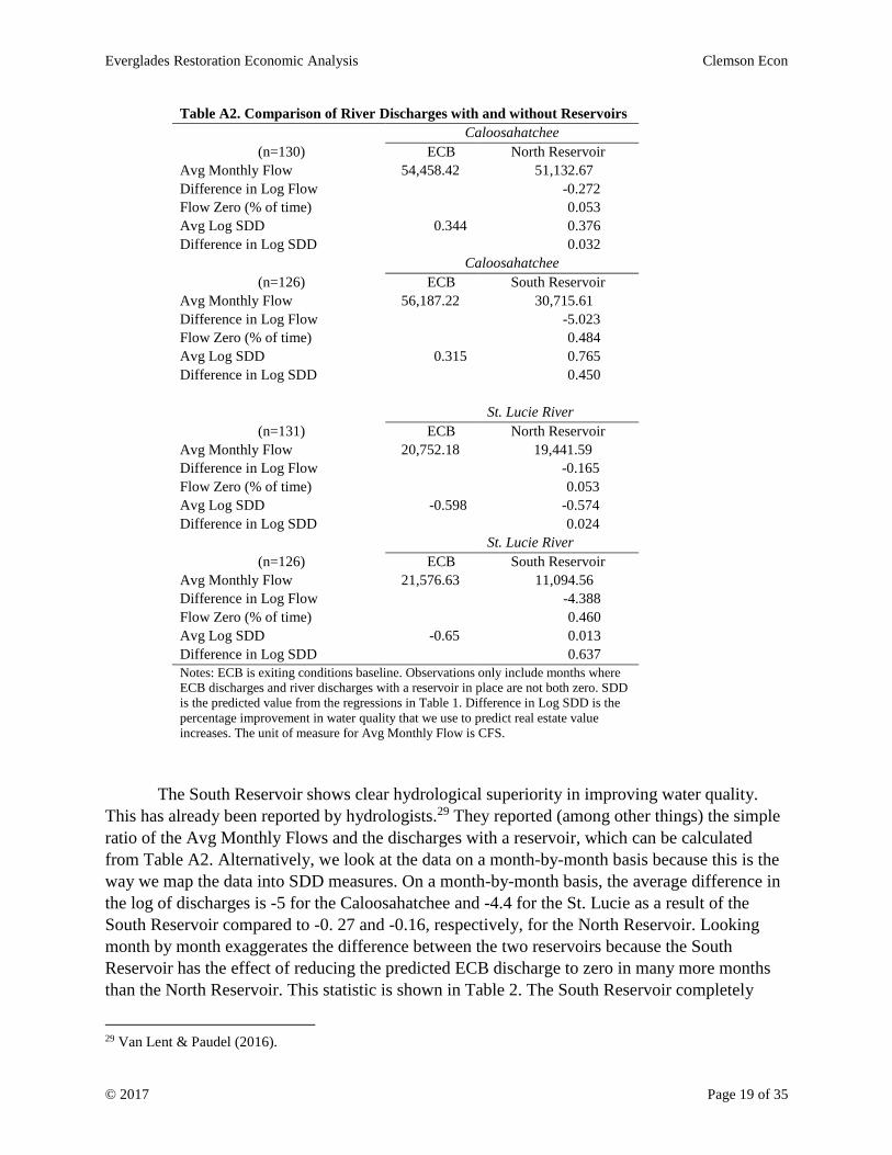
The results of this exercise are shown in Table A2. The first thing to notice in Table A2 is
that the ECB discharge levels are different for each reservoir for each river. This is because we
delete observations when there is no harmful discharge predicted.
Ultimately there are four values of interest. These are the Avg Difference in Log SDD,
which is the percentage improvement in water quality as measured by SDD, for the
Caloosahatchee and St. Lucie River, for the South Reservoir and for the North Reservoir. These
values shown in Table A2 are {0.45, 0.637, 0.032, 0.024} respectively.
Everglades Restoration Economic Analysis Clemson Econ
© 2017 Page 19 of 35
Table A2. Comparison of River Discharges with and without Reservoirs
Caloosahatchee
(n=130) ECB North Reservoir
Avg Monthly Flow 54,458.42 51,132.67
Difference in Log Flow -0.272
Flow Zero (% of time) 0.053
Avg Log SDD 0.344 0.376
Difference in Log SDD 0.032
Caloosahatchee
(n=126) ECB South Reservoir
Avg Monthly Flow 56,187.22 30,715.61
Difference in Log Flow -5.023
Flow Zero (% of time) 0.484
Avg Log SDD 0.315 0.765
Difference in Log SDD 0.450
St. Lucie River
(n=131) ECB North Reservoir
Avg Monthly Flow 20,752.18 19,441.59
Difference in Log Flow -0.165
Flow Zero (% of time) 0.053
Avg Log SDD -0.598 -0.574
Difference in Log SDD 0.024
St. Lucie River
(n=126) ECB South Reservoir
Avg Monthly Flow 21,576.63 11,094.56
Difference in Log Flow -4.388
Flow Zero (% of time) 0.460
Avg Log SDD -0.65 0.013
Difference in Log SDD 0.637
Notes: ECB is exiting conditions baseline. Observations only include months where
ECB discharges and river discharges with a reservoir in place are not both zero. SDD
is the predicted value from the regressions in Table 1. Difference in Log SDD is the
percentage improvement in water quality that we use to predict real estate value
increases. The unit of measure for Avg Monthly Flow is CFS.
The South Reservoir shows clear hydrological superiority in improving water quality.
This has already been reported by hydrologists.29 They reported (among other things) the simple
ratio of the Avg Monthly Flows and the discharges with a reservoir, which can be calculated
from Table A2. Alternatively, we look at the data on a month-by-month basis because this is the
way we map the data into SDD measures. On a month-by-month basis, the average difference in
the log of discharges is -5 for the Caloosahatchee and -4.4 for the St. Lucie as a result of the
South Reservoir compared to -0. 27 and -0.16, respectively, for the North Reservoir. Looking
month by month exaggerates the difference between the two reservoirs because the South
Reservoir has the effect of reducing the predicted ECB discharge to zero in many more months
than the North Reservoir. This statistic is shown in Table 2. The South Reservoir completely
29 Van Lent & Paudel (2016).
Everglades Restoration Economic Analysis Clemson Econ
© 2017 Page 20 of 35
eliminates harmful discharges nearly 50% of the time for both rivers while the North Reservoir
only produces this result around 5% of the time. Big discharges do the most damage to water
quality and reducing them to zero has the most beneficial effect.
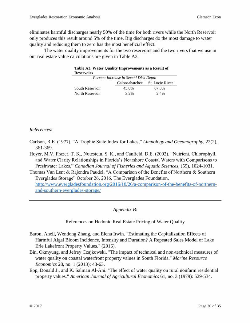
The water quality improvements for the two reservoirs and the two rivers that we use in
our real estate value calculations are given in Table A3.
Table A3. Water Quality Improvements as a Result of
Reservoirs
Percent Increase in Secchi Disk Depth
Caloosahatchee St. Lucie River
South Reservoir 45.0% 67.3%
North Reservoir 3.2% 2.4%
References:
Carlson, R.E. (1977). “A Trophic State Index for Lakes,” Limnology and Oceanography, 22(2),
361-369.
Hoyer, M.V, Frazer, T. K., Notestein, S. K., and Canfield, D.E. (2002). “Nutrient, Chlorophyll,
and Water Clarity Relationships in Florida’s Nearshore Coastal Waters with Comparisons to
Freshwater Lakes,” Canadian Journal of Fisheries and Aquatic Sciences, (59), 1024-1031.
Thomas Van Lent & Rajendra Paudel, “A Comparison of the Benefits of Northern & Southern
Everglades Storage” October 26, 2016, The Everglades Foundation,
http://www.evergladesfoundation.org/2016/10/26/a-comparison-of-the-benefits-of-northern-
and-southern-everglades-storage/
Appendix B:
References on Hedonic Real Estate Pricing of Water Quality
Baron, Aneil, Wendong Zhang, and Elena Irwin. "Estimating the Capitalization Effects of
Harmful Algal Bloom Incidence, Intensity and Duration? A Repeated Sales Model of Lake
Erie Lakefront Property Values." (2016).
Bin, Okmyung, and Jefrey Czajkowski. "The impact of technical and non-technical measures of
water quality on coastal waterfront property values in South Florida." Marine Resource
Economics 28, no. 1 (2013): 43-63.
Epp, Donald J., and K. Salman Al-Ani. "The effect of water quality on rural nonfarm residential
property values." American Journal of Agricultural Economics 61, no. 3 (1979): 529-534.
Everglades Restoration Economic Analysis Clemson Econ
© 2017 Page 21 of 35
Feather, Timothy D., Edward M. Pettit, and Panagiotis Ventikos. Valuation of lake resources
through hedonic pricing. No. IRW-92-R-8. ARMY ENGINEER INST FOR WATER
RESOURCES ALEXANDRIA VA, 1992.
Krysel, Charles, Elizabeth Marsh Boyer, Charles Parson, and Patrick Welle. "Lakeshore property
values and water quality: Evidence from property sales in the Mississippi Headwaters
Region." Submitted to the Legislative Commission on Minnesota Resources by the
Mississippi Headwaters Board and Bemidji State University (2003).
Leggett, Christopher G., and Nancy E. Bockstael. "Evidence of the effects of water quality on
residential land prices." Journal of Environmental Economics and Management 39, no. 2
(2000): 121-144.
Michael, Holly J., Kevin J. Boyle, and Roy Bouchard. "Does the measurement of environmental
quality affect implicit prices estimated from hedonic models?." Land Economics (2000): 283-
298.
Michael, Holly J., Kevin J. Boyle, and Roy Bouchard. "MR398: Water Quality Affects Property
Prices: A Case Study of Selected Maine Lakes." (1996).
Poor, P. Joan, Kevin J. Boyle, Laura O. Taylor, and Roy Bouchard. "Objective versus subjective
measures of water clarity in hedonic property value models." Land Economics 77, no. 4
(2001): 482-493.
Steinnes, Donald N. "Measuring the economic value of water quality." The Annals of Regional
Science 26, no. 2 (1992): 171-176.
Walsh, Patrick J., J. Walter Milon, and David O. Scrogin. "The spatial extent of water quality
benefits in urban housing markets." Land Economics 87, no. 4 (2011): 628-644.
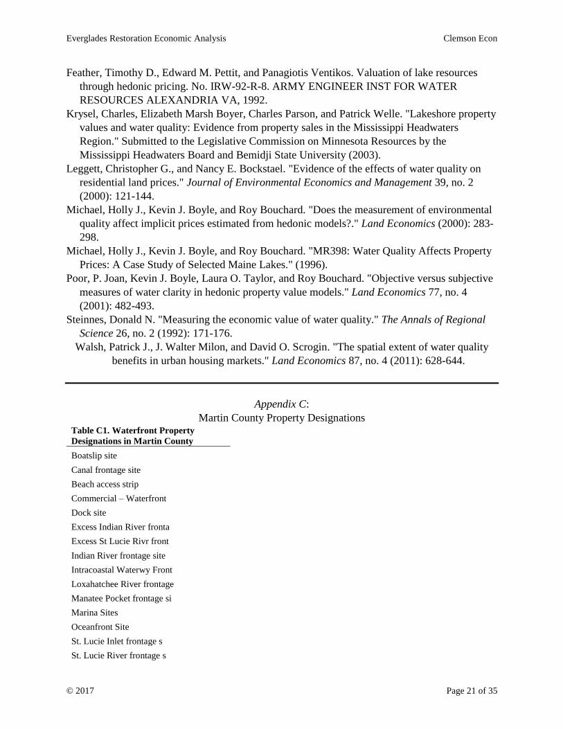
Appendix C:
Martin County Property Designations Table C1. Waterfront Property
Designations in Martin County
Boatslip site
Canal frontage site
Beach access strip
Commercial – Waterfront
Dock site
Excess Indian River fronta
Excess St Lucie Rivr front
Indian River frontage site
Intracoastal Waterwy Front
Loxahatchee River frontage
Manatee Pocket frontage si
Marina Sites
Oceanfront Site
St. Lucie Inlet frontage s
St. Lucie River frontage s
Everglades Restoration Economic Analysis Clemson Econ
© 2017 Page 22 of 35
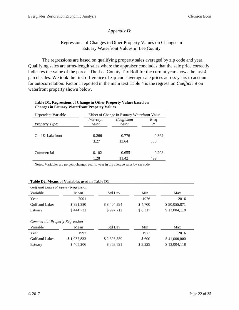
Appendix D:
Regressions of Changes in Other Property Values on Changes in
Estuary Waterfront Values in Lee County
The regressions are based on qualifying property sales averaged by zip code and year.
Qualifying sales are arms-length sales where the appraiser concludes that the sale price correctly
indicates the value of the parcel. The Lee County Tax Roll for the current year shows the last 4
parcel sales. We took the first difference of zip-code average sale prices across years to account
for autocorrelation. Factor 1 reported in the main text Table 4 is the regression Coefficient on
waterfront property shown below.
Table D1. Regressions of Change in Other Property Values based on
Changes in Estuary Waterfront Property Values
Dependent Variable Effect of Change in Estuary Waterfront Value
Property Type:
Intercept
t-stat
Coefficient
t-stat
R-sq
N
Golf & Lakefront 0.266 0.776 0.362
3.27 13.64 330
Commercial 0.102 0.655 0.208
1.28 11.42 499
Notes: Variables are percent changes year to year in the average sales by zip code
Table D2. Means of Variables used in Table D1
Golf and Lakes Property Regression
Variable Mean Std Dev Min Max
Year 2001 1976 2016
Golf and Lakes $ 891,380 $ 3,404,594 $ 4,700 $ 50,055,871
Estuary $ 444,731 $ 997,712 $ 6,317 $ 13,004,118
Commercial Property Regression
Variable Mean Std Dev Min Max
Year 1997 1973 2016
Golf and Lakes $ 1,037,833 $ 2,626,559 $ 600 $ 41,000,000
Estuary $ 405,206 $ 863,891 $ 3,225 $ 13,004,118
Everglades Restoration Economic Analysis Clemson Econ
© 2017 Page 23 of 35
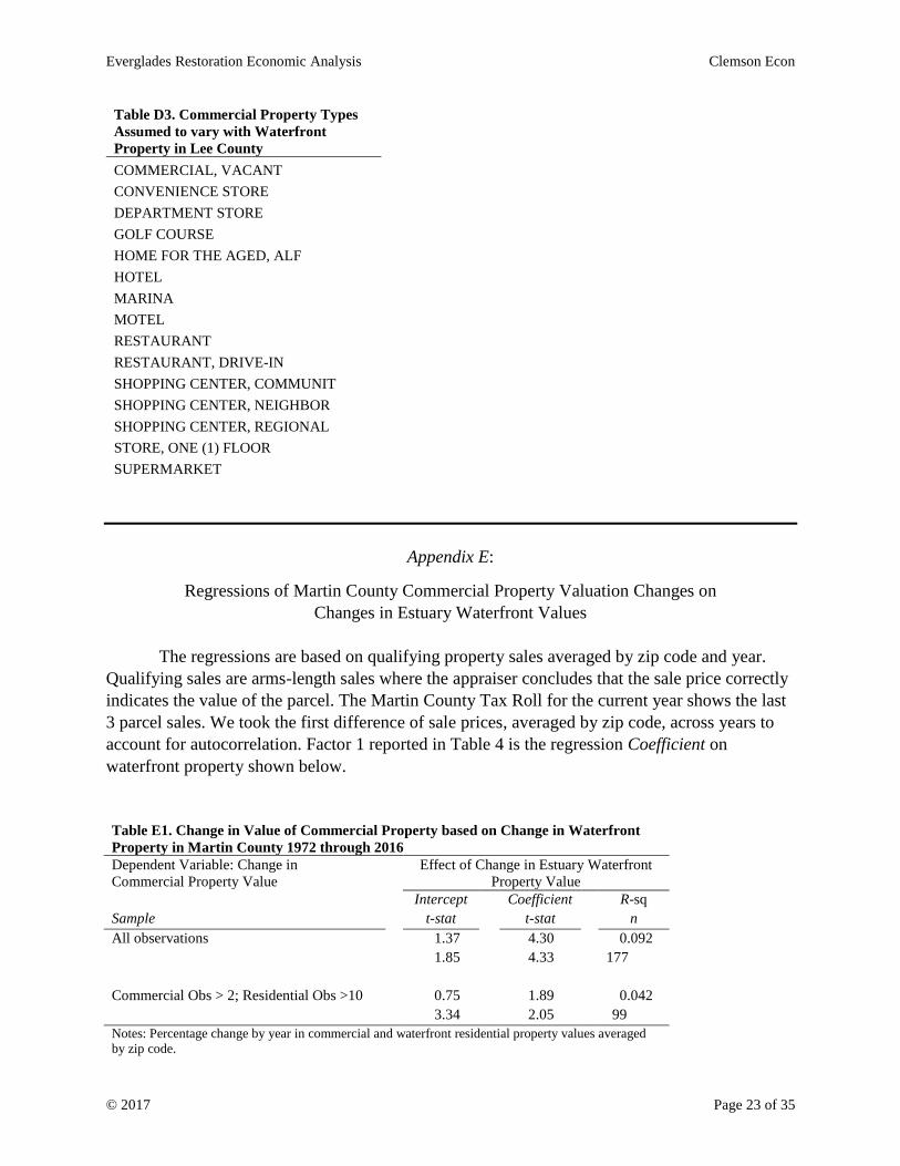
Table D3. Commercial Property Types
Assumed to vary with Waterfront
Property in Lee County
COMMERCIAL, VACANT
CONVENIENCE STORE
DEPARTMENT STORE
GOLF COURSE
HOME FOR THE AGED, ALF
HOTEL
MARINA
MOTEL
RESTAURANT
RESTAURANT, DRIVE-IN
SHOPPING CENTER, COMMUNIT
SHOPPING CENTER, NEIGHBOR
SHOPPING CENTER, REGIONAL
STORE, ONE (1) FLOOR
SUPERMARKET
Appendix E:
Regressions of Martin County Commercial Property Valuation Changes on
Changes in Estuary Waterfront Values
The regressions are based on qualifying property sales averaged by zip code and year.
Qualifying sales are arms-length sales where the appraiser concludes that the sale price correctly
indicates the value of the parcel. The Martin County Tax Roll for the current year shows the last
3 parcel sales. We took the first difference of sale prices, averaged by zip code, across years to
account for autocorrelation. Factor 1 reported in Table 4 is the regression Coefficient on
waterfront property shown below.
Table E1. Change in Value of Commercial Property based on Change in Waterfront
Property in Martin County 1972 through 2016
Dependent Variable: Change in
Commercial Property Value
Effect of Change in Estuary Waterfront
Property Value
Intercept Coefficient R-sq
Sample t-stat t-stat n
All observations 1.37 4.30 0.092
1.85 4.33 177
Commercial Obs > 2; Residential Obs >10 0.75 1.89 0.042
3.34 2.05 99
Notes: Percentage change by year in commercial and waterfront residential property values averaged
by zip code.
Everglades Restoration Economic Analysis Clemson Econ
© 2017 Page 24 of 35
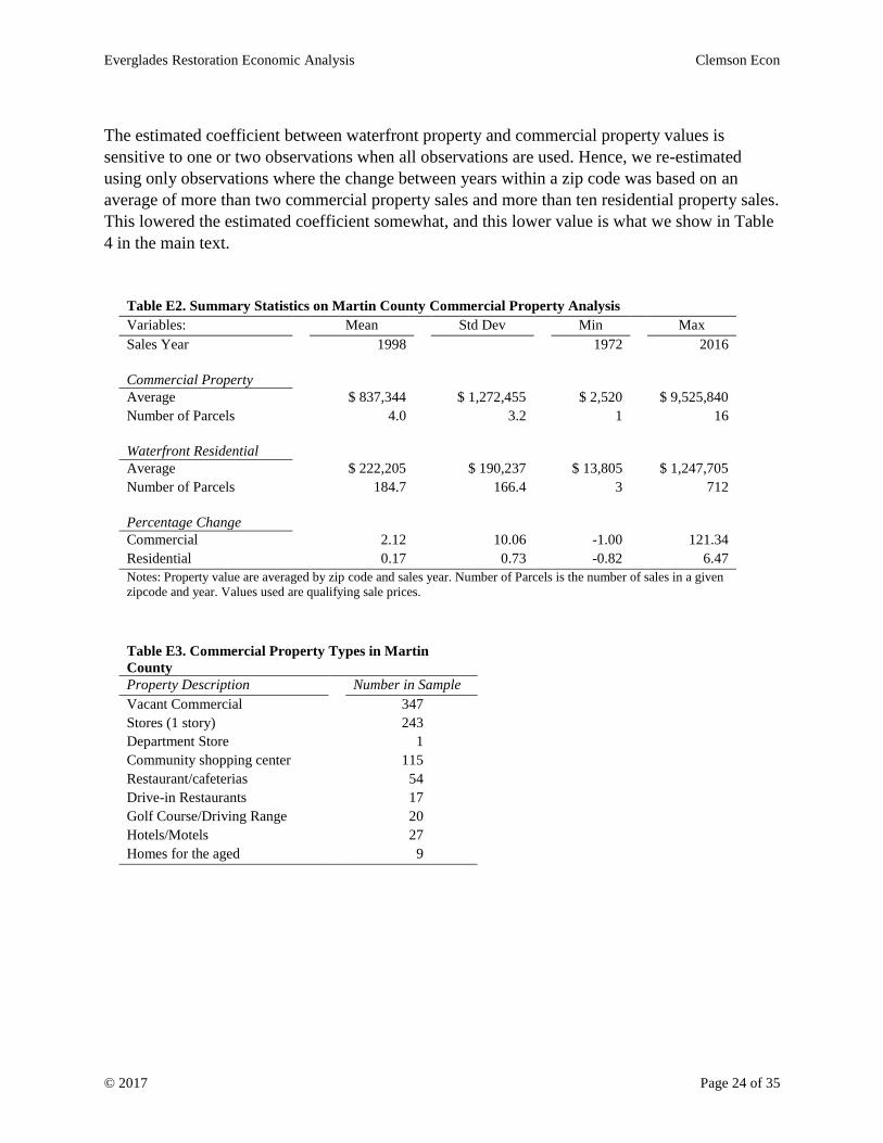
The estimated coefficient between waterfront property and commercial property values is
sensitive to one or two observations when all observations are used. Hence, we re-estimated
using only observations where the change between years within a zip code was based on an
average of more than two commercial property sales and more than ten residential property sales.
This lowered the estimated coefficient somewhat, and this lower value is what we show in Table
4 in the main text.
Table E2. Summary Statistics on Martin County Commercial Property Analysis
Variables: Mean Std Dev Min Max
Sales Year 1998 1972 2016
Commercial Property
Average $ 837,344 $ 1,272,455 $ 2,520 $ 9,525,840
Number of Parcels 4.0 3.2 1 16
Waterfront Residential
Average $ 222,205 $ 190,237 $ 13,805 $ 1,247,705
Number of Parcels 184.7 166.4 3 712
Percentage Change
Commercial 2.12 10.06 -1.00 121.34
Residential 0.17 0.73 -0.82 6.47
Notes: Property value are averaged by zip code and sales year. Number of Parcels is the number of sales in a given
zipcode and year. Values used are qualifying sale prices.
Table E3. Commercial Property Types in Martin
County
Property Description Number in Sample
Vacant Commercial 347
Stores (1 story) 243
Department Store 1
Community shopping center 115
Restaurant/cafeterias 54
Drive-in Restaurants 17
Golf Course/Driving Range 20
Hotels/Motels 27
Homes for the aged 9
Everglades Restoration Economic Analysis Clemson Econ
© 2017 Page 25 of 35
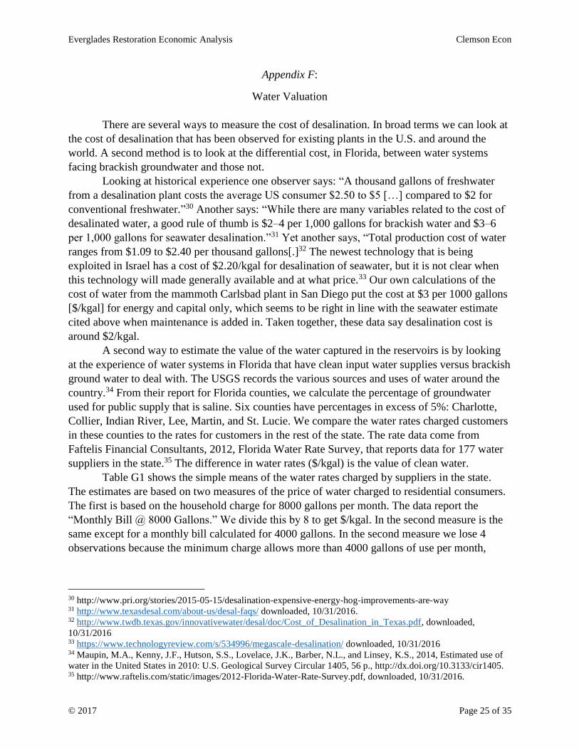
Appendix F:
Water Valuation
There are several ways to measure the cost of desalination. In broad terms we can look at
the cost of desalination that has been observed for existing plants in the U.S. and around the
world. A second method is to look at the differential cost, in Florida, between water systems
facing brackish groundwater and those not.
Looking at historical experience one observer says: “A thousand gallons of freshwater
from a desalination plant costs the average US consumer $2.50 to $5 […] compared to $2 for
conventional freshwater.”30 Another says: “While there are many variables related to the cost of
desalinated water, a good rule of thumb is $2–4 per 1,000 gallons for brackish water and $3–6
per 1,000 gallons for seawater desalination.”31 Yet another says, “Total production cost of water
ranges from $1.09 to $2.40 per thousand gallons[.]32 The newest technology that is being
exploited in Israel has a cost of $2.20/kgal for desalination of seawater, but it is not clear when
this technology will made generally available and at what price.33 Our own calculations of the
cost of water from the mammoth Carlsbad plant in San Diego put the cost at $3 per 1000 gallons
[$/kgal] for energy and capital only, which seems to be right in line with the seawater estimate
cited above when maintenance is added in. Taken together, these data say desalination cost is
around $2/kgal.
A second way to estimate the value of the water captured in the reservoirs is by looking
at the experience of water systems in Florida that have clean input water supplies versus brackish
ground water to deal with. The USGS records the various sources and uses of water around the
country.34 From their report for Florida counties, we calculate the percentage of groundwater
used for public supply that is saline. Six counties have percentages in excess of 5%: Charlotte,
Collier, Indian River, Lee, Martin, and St. Lucie. We compare the water rates charged customers
in these counties to the rates for customers in the rest of the state. The rate data come from
Faftelis Financial Consultants, 2012, Florida Water Rate Survey, that reports data for 177 water
suppliers in the state.35 The difference in water rates ($/kgal) is the value of clean water.
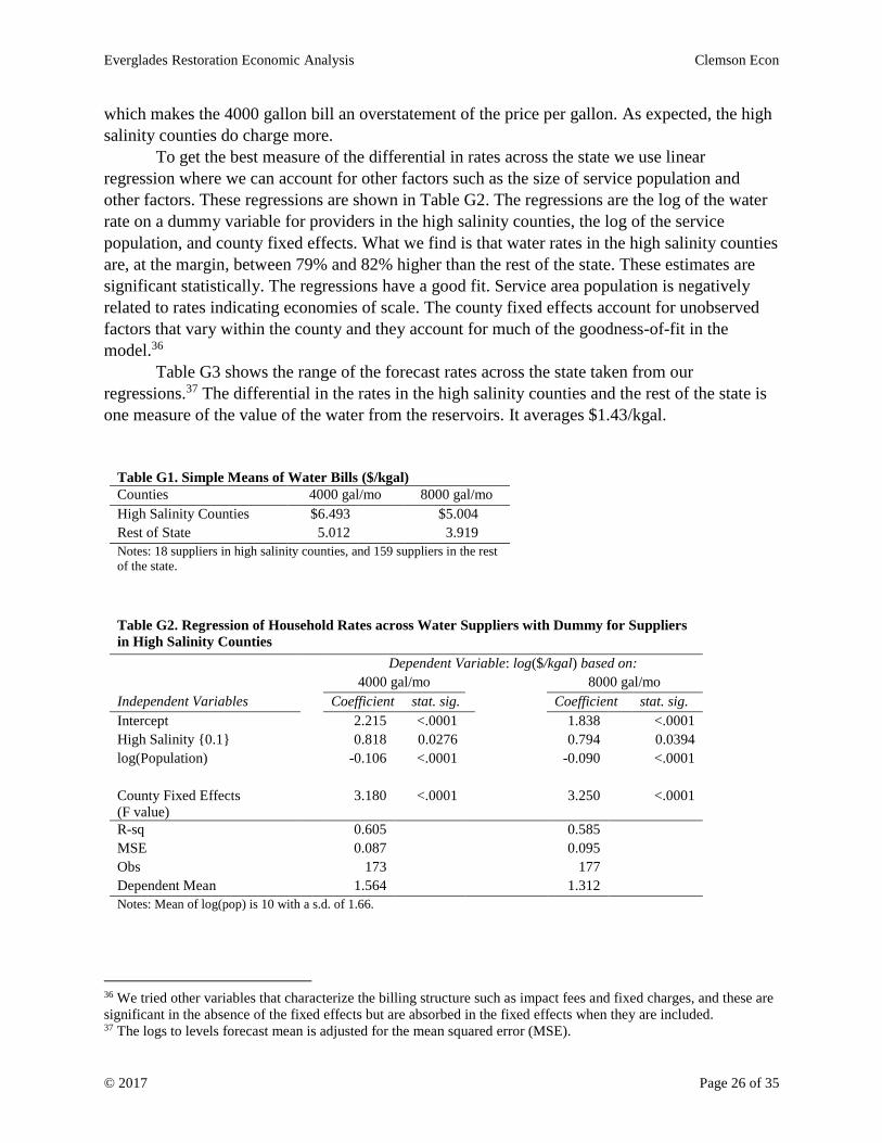
Table G1 shows the simple means of the water rates charged by suppliers in the state.
The estimates are based on two measures of the price of water charged to residential consumers.
The first is based on the household charge for 8000 gallons per month. The data report the
“Monthly Bill @ 8000 Gallons.” We divide this by 8 to get $/kgal. In the second measure is the
same except for a monthly bill calculated for 4000 gallons. In the second measure we lose 4
observations because the minimum charge allows more than 4000 gallons of use per month,
30 http://www.pri.org/stories/2015-05-15/desalination-expensive-energy-hog-improvements-are-way 31 http://www.texasdesal.com/about-us/desal-faqs/ downloaded, 10/31/2016. 32 http://www.twdb.texas.gov/innovativewater/desal/doc/Cost_of_Desalination_in_Texas.pdf, downloaded,
10/31/2016 33 https://www.technologyreview.com/s/534996/megascale-desalination/ downloaded, 10/31/2016 34 Maupin, M.A., Kenny, J.F., Hutson, S.S., Lovelace, J.K., Barber, N.L., and Linsey, K.S., 2014, Estimated use of
water in the United States in 2010: U.S. Geological Survey Circular 1405, 56 p., http://dx.doi.org/10.3133/cir1405. 35 http://www.raftelis.com/static/images/2012-Florida-Water-Rate-Survey.pdf, downloaded, 10/31/2016.
Everglades Restoration Economic Analysis Clemson Econ
© 2017 Page 26 of 35
which makes the 4000 gallon bill an overstatement of the price per gallon. As expected, the high
salinity counties do charge more.
To get the best measure of the differential in rates across the state we use linear
regression where we can account for other factors such as the size of service population and
other factors. These regressions are shown in Table G2. The regressions are the log of the water
rate on a dummy variable for providers in the high salinity counties, the log of the service
population, and county fixed effects. What we find is that water rates in the high salinity counties
are, at the margin, between 79% and 82% higher than the rest of the state. These estimates are
significant statistically. The regressions have a good fit. Service area population is negatively
related to rates indicating economies of scale. The county fixed effects account for unobserved
factors that vary within the county and they account for much of the goodness-of-fit in the
model.36
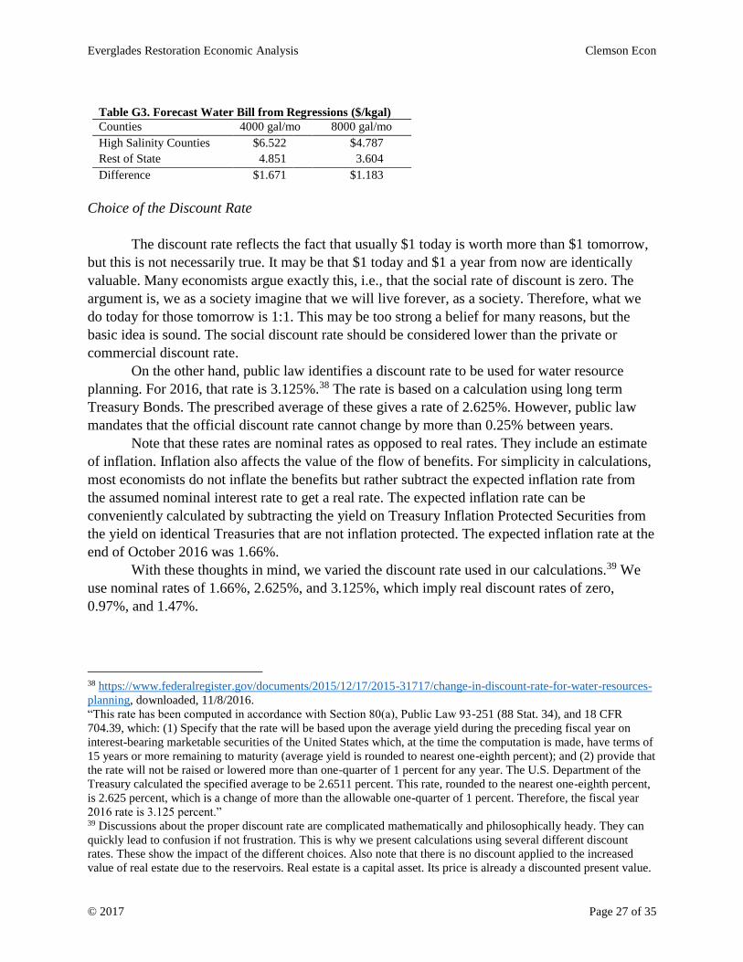
Table G3 shows the range of the forecast rates across the state taken from our
regressions.37 The differential in the rates in the high salinity counties and the rest of the state is
one measure of the value of the water from the reservoirs. It averages $1.43/kgal.
Table G1. Simple Means of Water Bills ($/kgal)
Counties 4000 gal/mo 8000 gal/mo
High Salinity Counties $6.493 $5.004
Rest of State 5.012 3.919
Notes: 18 suppliers in high salinity counties, and 159 suppliers in the rest
of the state.
Table G2. Regression of Household Rates across Water Suppliers with Dummy for Suppliers
in High Salinity Counties
Dependent Variable: log($/kgal) based on:
4000 gal/mo 8000 gal/mo
Independent Variables Coefficient stat. sig. Coefficient stat. sig.
Intercept 2.215 <.0001 1.838 <.0001
High Salinity {0.1} 0.818 0.0276 0.794 0.0394
log(Population) -0.106 <.0001 -0.090 <.0001
County Fixed Effects
(F value)
3.180 <.0001 3.250 <.0001
R-sq 0.605 0.585
MSE 0.087 0.095
Obs 173 177
Dependent Mean 1.564 1.312
Notes: Mean of log(pop) is 10 with a s.d. of 1.66.
36 We tried other variables that characterize the billing structure such as impact fees and fixed charges, and these are
significant in the absence of the fixed effects but are absorbed in the fixed effects when they are included. 37 The logs to levels forecast mean is adjusted for the mean squared error (MSE).
Everglades Restoration Economic Analysis Clemson Econ
© 2017 Page 27 of 35
Table G3. Forecast Water Bill from Regressions ($/kgal)
Counties 4000 gal/mo 8000 gal/mo
High Salinity Counties $6.522 $4.787
Rest of State 4.851 3.604
Difference $1.671 $1.183
Choice of the Discount Rate
The discount rate reflects the fact that usually $1 today is worth more than $1 tomorrow,
but this is not necessarily true. It may be that $1 today and $1 a year from now are identically
valuable. Many economists argue exactly this, i.e., that the social rate of discount is zero. The
argument is, we as a society imagine that we will live forever, as a society. Therefore, what we
do today for those tomorrow is 1:1. This may be too strong a belief for many reasons, but the
basic idea is sound. The social discount rate should be considered lower than the private or
commercial discount rate.
On the other hand, public law identifies a discount rate to be used for water resource
planning. For 2016, that rate is 3.125%.38 The rate is based on a calculation using long term
Treasury Bonds. The prescribed average of these gives a rate of 2.625%. However, public law
mandates that the official discount rate cannot change by more than 0.25% between years.
Note that these rates are nominal rates as opposed to real rates. They include an estimate
of inflation. Inflation also affects the value of the flow of benefits. For simplicity in calculations,
most economists do not inflate the benefits but rather subtract the expected inflation rate from
the assumed nominal interest rate to get a real rate. The expected inflation rate can be
conveniently calculated by subtracting the yield on Treasury Inflation Protected Securities from
the yield on identical Treasuries that are not inflation protected. The expected inflation rate at the
end of October 2016 was 1.66%.
With these thoughts in mind, we varied the discount rate used in our calculations.39 We
use nominal rates of 1.66%, 2.625%, and 3.125%, which imply real discount rates of zero,
0.97%, and 1.47%.
38 https://www.federalregister.gov/documents/2015/12/17/2015-31717/change-in-discount-rate-for-water-resources-
planning, downloaded, 11/8/2016.
“This rate has been computed in accordance with Section 80(a), Public Law 93-251 (88 Stat. 34), and 18 CFR
704.39, which: (1) Specify that the rate will be based upon the average yield during the preceding fiscal year on
interest-bearing marketable securities of the United States which, at the time the computation is made, have terms of
15 years or more remaining to maturity (average yield is rounded to nearest one-eighth percent); and (2) provide that
the rate will not be raised or lowered more than one-quarter of 1 percent for any year. The U.S. Department of the
Treasury calculated the specified average to be 2.6511 percent. This rate, rounded to the nearest one-eighth percent,
is 2.625 percent, which is a change of more than the allowable one-quarter of 1 percent. Therefore, the fiscal year
2016 rate is 3.125 percent.” 39 Discussions about the proper discount rate are complicated mathematically and philosophically heady. They can
quickly lead to confusion if not frustration. This is why we present calculations using several different discount
rates. These show the impact of the different choices. Also note that there is no discount applied to the increased
value of real estate due to the reservoirs. Real estate is a capital asset. Its price is already a discounted present value.
Everglades Restoration Economic Analysis Clemson Econ
© 2017 Page 28 of 35
Jobs Calculations for Two Everglades Restoration Projects
Michael T. Maloney
Emeritus Professor of Economics
Clemson University40
Introduction
The purpose of this report is to calculate the economic benefits in terms of jobs created
by the construction of two alternative Everglades restoration projects. We call one the South
Reservoir, a reservoir south of Lake Okeechobee that would provide storage when the lake is too
full. The other is called the North Reservoir, a storage area north of Lake Okeechobee that will
capture water before it enters the lake. One purpose of the reservoirs is to mitigate the discharge
of the excess water from Lake Okeechobee into the St. Lucie River and the Caloosahatchee
where it damages the estuaries and negatively affects water quality.
In an earlier study, we report details of the effect of the alternative reservoirs on water
quality and calculate the increase in the value of existing real estate that would result from
improved water quality.41 The increase in the value of existing real estate will cause new
construction of residential and commercial real estate. This new construction will create new
jobs. The construction of the reservoirs themselves will create new jobs. This reports measures
these employment effects.
Prior Research
The prior study shows that the South Reservoir outperforms the alternative of a North
Reservoir, improving water quality by more than 45% in the Caloosahatchee and 64% in the St.
Lucie River. This will cause property values of homes on or near the waterfront to increase by
18%, resulting in over $12 billion in increased value. Properties related to and serving those
homes are also expected to increase in value, adding about $6.5 billion in value. There’s also
value in the water to be collected in the reservoir that would otherwise be dumped into the seas.
Adding this to the increased real estate value, the benefits of the South Reservoir are expected to
be over $20 billion. The cost of the South Reservoir is estimated to be about $2.5 billion, so the
net benefits are over $17 billion with a benefit-cost ratio of 8.1.
The North Reservoir is not nearly so effective at reducing discharges to the estuaries, and,
hence, will have economically less effect. It will only result in discharge mitigation of 5-6%.
Benefits, counting the value of the water, would be $1.7 billion with a benefits-cost ratio of 1.5.
The table with the cost-benefit conclusions is reproduced below.
40 Contact: [email protected]; web: maloney.people.clemson.edu 41 “Benefit & Benefit/Cost Calculations for Two Everglades Restoration Projects,” Michael T. Maloney, Charles J.
Thomas, Babur De Los Santos, Amanda J. Hobbs, Kathryn Sauer, and John Parker, 2/18/2017, Everglades
Foundation.
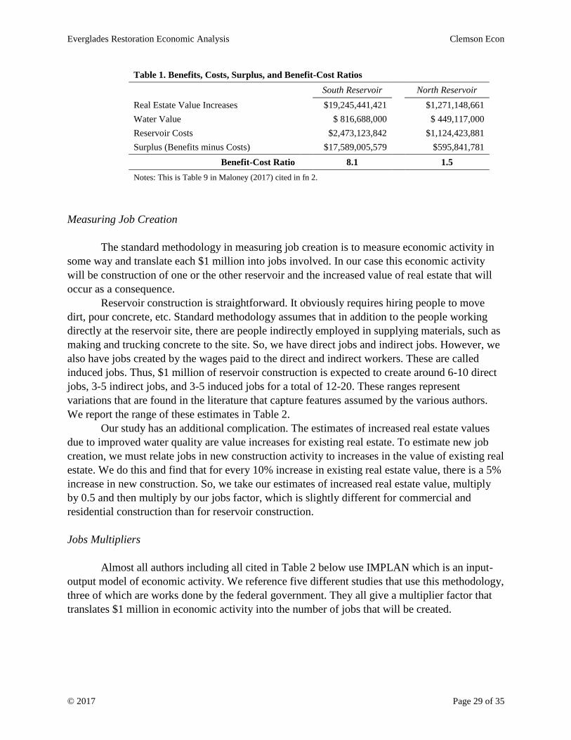
Everglades Restoration Economic Analysis Clemson Econ
© 2017 Page 29 of 35
Table 1. Benefits, Costs, Surplus, and Benefit-Cost Ratios
South Reservoir North Reservoir
Real Estate Value Increases $19,245,441,421 $1,271,148,661
Water Value $ 816,688,000 $ 449,117,000
Reservoir Costs $2,473,123,842 $1,124,423,881
Surplus (Benefits minus Costs) $17,589,005,579 $595,841,781
Benefit-Cost Ratio 8.1 1.5
Notes: This is Table 9 in Maloney (2017) cited in fn 2.
Measuring Job Creation
The standard methodology in measuring job creation is to measure economic activity in
some way and translate each $1 million into jobs involved. In our case this economic activity
will be construction of one or the other reservoir and the increased value of real estate that will
occur as a consequence.
Reservoir construction is straightforward. It obviously requires hiring people to move
dirt, pour concrete, etc. Standard methodology assumes that in addition to the people working
directly at the reservoir site, there are people indirectly employed in supplying materials, such as
making and trucking concrete to the site. So, we have direct jobs and indirect jobs. However, we
also have jobs created by the wages paid to the direct and indirect workers. These are called
induced jobs. Thus, $1 million of reservoir construction is expected to create around 6-10 direct
jobs, 3-5 indirect jobs, and 3-5 induced jobs for a total of 12-20. These ranges represent
variations that are found in the literature that capture features assumed by the various authors.
We report the range of these estimates in Table 2.
Our study has an additional complication. The estimates of increased real estate values
due to improved water quality are value increases for existing real estate. To estimate new job
creation, we must relate jobs in new construction activity to increases in the value of existing real
estate. We do this and find that for every 10% increase in existing real estate value, there is a 5%
increase in new construction. So, we take our estimates of increased real estate value, multiply
by 0.5 and then multiply by our jobs factor, which is slightly different for commercial and
residential construction than for reservoir construction.
Jobs Multipliers
Almost all authors including all cited in Table 2 below use IMPLAN which is an input-
output model of economic activity. We reference five different studies that use this methodology,
three of which are works done by the federal government. They all give a multiplier factor that
translates $1 million in economic activity into the number of jobs that will be created.
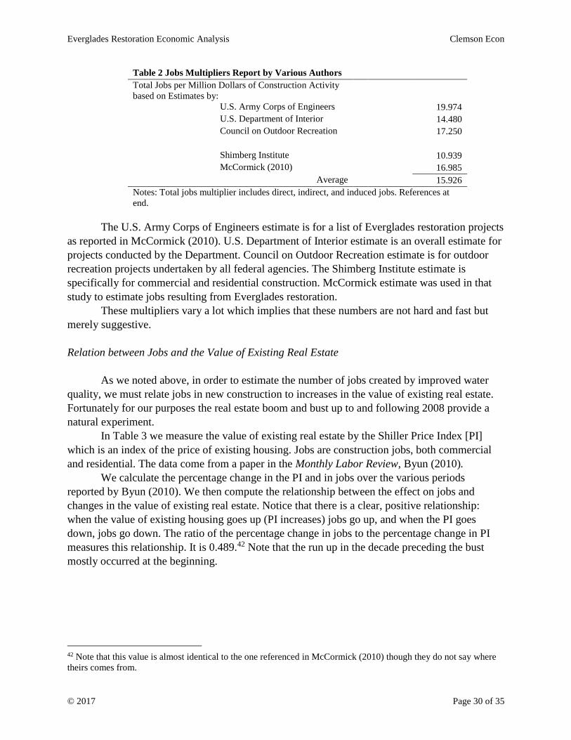
Everglades Restoration Economic Analysis Clemson Econ
© 2017 Page 30 of 35
Table 2 Jobs Multipliers Report by Various Authors
Total Jobs per Million Dollars of Construction Activity
based on Estimates by:
U.S. Army Corps of Engineers 19.974
U.S. Department of Interior 14.480
Council on Outdoor Recreation 17.250
Shimberg Institute 10.939
McCormick (2010) 16.985
Average 15.926
Notes: Total jobs multiplier includes direct, indirect, and induced jobs. References at
end.
The U.S. Army Corps of Engineers estimate is for a list of Everglades restoration projects
as reported in McCormick (2010). U.S. Department of Interior estimate is an overall estimate for
projects conducted by the Department. Council on Outdoor Recreation estimate is for outdoor
recreation projects undertaken by all federal agencies. The Shimberg Institute estimate is
specifically for commercial and residential construction. McCormick estimate was used in that
study to estimate jobs resulting from Everglades restoration.
These multipliers vary a lot which implies that these numbers are not hard and fast but
merely suggestive.
Relation between Jobs and the Value of Existing Real Estate
As we noted above, in order to estimate the number of jobs created by improved water
quality, we must relate jobs in new construction to increases in the value of existing real estate.
Fortunately for our purposes the real estate boom and bust up to and following 2008 provide a
natural experiment.
In Table 3 we measure the value of existing real estate by the Shiller Price Index [PI]
which is an index of the price of existing housing. Jobs are construction jobs, both commercial
and residential. The data come from a paper in the Monthly Labor Review, Byun (2010).
We calculate the percentage change in the PI and in jobs over the various periods
reported by Byun (2010). We then compute the relationship between the effect on jobs and
changes in the value of existing real estate. Notice that there is a clear, positive relationship:
when the value of existing housing goes up (PI increases) jobs go up, and when the PI goes
down, jobs go down. The ratio of the percentage change in jobs to the percentage change in PI
measures this relationship. It is 0.489.42 Note that the run up in the decade preceding the bust
mostly occurred at the beginning.
42 Note that this value is almost identical to the one referenced in McCormick (2010) though they do not say where
theirs comes from.
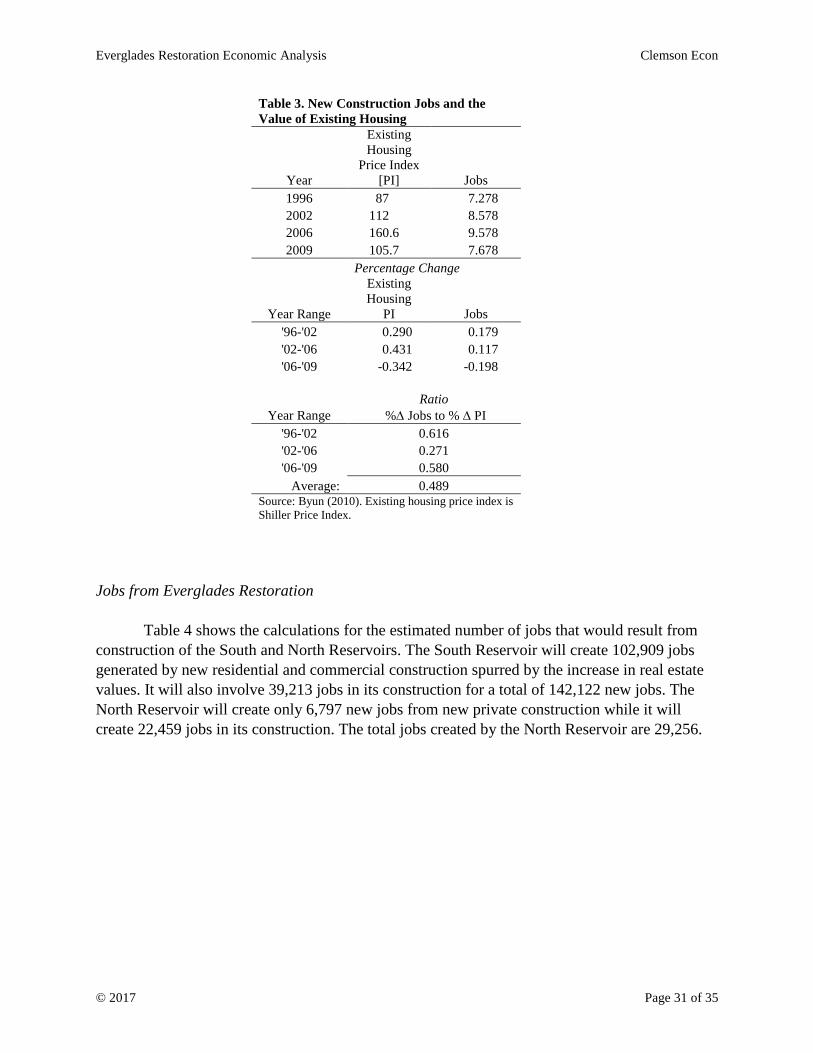
Everglades Restoration Economic Analysis Clemson Econ
© 2017 Page 31 of 35
Table 3. New Construction Jobs and the
Value of Existing Housing
Year
Existing
Housing
Price Index
[PI] Jobs
1996 87 7.278
2002 112 8.578
2006 160.6 9.578
2009 105.7 7.678
Percentage Change
Year Range
Existing
Housing
PI Jobs
'96-'02 0.290 0.179
'02-'06 0.431 0.117
'06-'09 -0.342 -0.198
Year Range
Ratio
% Jobs to % PI
'96-'02 0.616
'02-'06 0.271
'06-'09 0.580
Average: 0.489 Source: Byun (2010). Existing housing price index is
Shiller Price Index.
Jobs from Everglades Restoration
Table 4 shows the calculations for the estimated number of jobs that would result from
construction of the South and North Reservoirs. The South Reservoir will create 102,909 jobs
generated by new residential and commercial construction spurred by the increase in real estate
values. It will also involve 39,213 jobs in its construction for a total of 142,122 new jobs. The
North Reservoir will create only 6,797 new jobs from new private construction while it will
create 22,459 jobs in its construction. The total jobs created by the North Reservoir are 29,256.
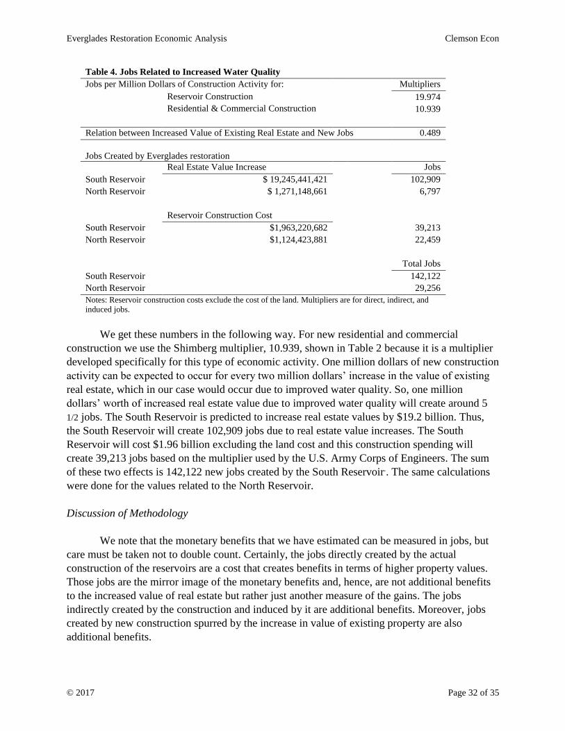
Everglades Restoration Economic Analysis Clemson Econ
© 2017 Page 32 of 35
Table 4. Jobs Related to Increased Water Quality
Jobs per Million Dollars of Construction Activity for: Multipliers
Reservoir Construction 19.974
Residential & Commercial Construction 10.939
Relation between Increased Value of Existing Real Estate and New Jobs 0.489
Jobs Created by Everglades restoration
Real Estate Value Increase Jobs
South Reservoir $ 19,245,441,421 102,909
North Reservoir $ 1,271,148,661 6,797
Reservoir Construction Cost
South Reservoir $1,963,220,682 39,213
North Reservoir $1,124,423,881 22,459
Total Jobs
South Reservoir 142,122
North Reservoir 29,256
Notes: Reservoir construction costs exclude the cost of the land. Multipliers are for direct, indirect, and
induced jobs.
We get these numbers in the following way. For new residential and commercial
construction we use the Shimberg multiplier, 10.939, shown in Table 2 because it is a multiplier
developed specifically for this type of economic activity. One million dollars of new construction
activity can be expected to occur for every two million dollars’ increase in the value of existing
real estate, which in our case would occur due to improved water quality. So, one million
dollars’ worth of increased real estate value due to improved water quality will create around 5
1/2 jobs. The South Reservoir is predicted to increase real estate values by $19.2 billion. Thus,
the South Reservoir will create 102,909 jobs due to real estate value increases. The South
Reservoir will cost $1.96 billion excluding the land cost and this construction spending will
create 39,213 jobs based on the multiplier used by the U.S. Army Corps of Engineers. The sum
of these two effects is 142,122 new jobs created by the South Reservoir.. The same calculations
were done for the values related to the North Reservoir.
Discussion of Methodology
We note that the monetary benefits that we have estimated can be measured in jobs, but
care must be taken not to double count. Certainly, the jobs directly created by the actual
construction of the reservoirs are a cost that creates benefits in terms of higher property values.
Those jobs are the mirror image of the monetary benefits and, hence, are not additional benefits
to the increased value of real estate but rather just another measure of the gains. The jobs
indirectly created by the construction and induced by it are additional benefits. Moreover, jobs
created by new construction spurred by the increase in value of existing property are also
additional benefits.
Everglades Restoration Economic Analysis Clemson Econ
© 2017 Page 33 of 35
Still some caveat is in order. Since the people employed in this new construction would
have been employed otherwise, the benefit is the net improvement in their income. Of course,
there is net improvement for the people who move into the jobs vacated by the people taking the
new jobs, and this effect passes on down the line. Economists have a (complicated) way of
measuring all this, but non-economists generally and intuitively understand that “new jobs” are a
measure of economic improvement but not in the full amount of the total income earned by the
new job holders. Hence, in this report we follow the convention adopted by policy makers and
talk about “jobs” as a benefit of these kinds of projects, but without trying to put an exact dollar
figure on it.
Jobs Lost
Some investigators have argued that the construction of Everglades restoration reservoirs
will cause a loss of jobs because it takes farm land out of production. Most recently this
proposition has been promoted in Villamil/JMI (2017) in regard to the South Reservoir.43
Villamil says that the total economic impact of the 60,000 acre acquisition for the South
Reservoir will cost 4,148 jobs state wide, which includes the direct loss of 1,915 jobs. In Table 8,
he says that the loss of jobs in agriculture in the counties where the reservoir would likely be
sited (these are the actual farm workers who would lose their jobs) is 890. This is not likely: 890
workers on 60,000 acres is 14.8 workers per 1000 acres. This would correspond to agricultural
productivity of more than a half-century ago not today’s.44
A detailed LSU study sugarcane production in 2014 found that the labor necessary to
farm 1000 acres was 5380 person hours, which at 2000 hours per year translates into 2.7 workers
per year.45 The study breaks production of a 1000 acre field into a 5 year rotation of seed
growing and annual harvesting.46 The study breaks the type of labor into field hands and more
specialized workers doing things like mechanical planting, harvesting, and hauling to the mill.
Hours per acre per year are detailed for each activity and each type of worker. The bottom line is
43 J. Antonio Villamil, “Sticker Shock, Examining the Economic Impacts of Land Acquisition in the EAA,” The
James Madison Institute, 2017. 44 For example, see “Farm Labor: No Easy Task,” Jim Simon, http://www.amscl.org/news/farm-labor-no-easy-task,
3/24/2014. Also note that a State of Texas census of agriculture from 1888 found that workers per 1000 acres for
crops like sugarcane was 34. Villamil’s estimates imply that labor productivity has only increased by a factor of 2.3
in the last 130 years. Yet we know that overall, farm labor productivity per acre increased by a factor of 3 since
1948. USDA, Economic Research Service, Productivity in the United States data product, updated December 2015,
Table 1a. 45 Salassi, Deliberto and Hilbun (2014). See also, Gravois (2014). 46 Salassi, et al., (2014). The authors calculate the cost and returns to a prototypical farm, and say, “Its structure
contains 20 percent plantcane, 20 percent first stubble, 20 percent second stubble, 20 percent 3rd stubble and 20
percent fallow/plant. Purchased cultured seedcane is expanded twice before being planted as millable cane
(plantcane only used for sevfed), with its first and second stubble being grown for sugar. One acre of propagated
seed cane is harvested and used for seed for each five acres to be planted. The cost and yield information used in the
illustration comes from tables 4, 5, 6, 8, 9, 11, 12, 13, and 14.” p. 28. Our calculations on farm labor come from
these tables.
Everglades Restoration Economic Analysis Clemson Econ
© 2017 Page 34 of 35
5380 person hours and $62,899 of labor cost (including 27.65% in benefit costs) per year for
1000 acres.47
If we apply the LSU analysis to the 60,000 acre South Reservoir track, the direct estimate
of the number of workers affected is 161 people, not 890. Villamil/JMI overstates the number of
directly affected jobs by more than 5 times. Possibly, though the study does not tell the reader,
the estimate includes sugarcane mill workers. This would be odd if true, because those jobs in
IMPLAN terms should be indirect jobs, i.e., workers not affected by production on the actual
site. Even so, we can again use the LSU study to see how much this affects the results. The LSU
study says that milling represents 39% of the cost of sugarcane production. So, if labor
productivity is the same in milling as working in the field, milling adds 1.7 workers per 1000
acres for a total of 4.4, or 265 for the 60,000 acre track in question.48 Again, this is a far cry from
890 workers.
The whole discussion of the economic impact of taking farm land out of production is
fundamentally based on the number of jobs actually lost. If the number of jobs actually lost
because of the construction of the 60,000 acre South Reservoir is 161 and not 890, then all the
other results in the Villamil/JMI study have to be discounted by 161/890, a factor of 5.5. So, for
example, the total economic impact of $695 million predicted to be lost because of the
construction is really $126 million, and the estimated 4148 total jobs lost state-wide is much
more likely 752, which is trivial compared to 142,122 jobs created by the South Reservoir.
The Villamil/JMI exercise is actually informative. It tells us how careful we must be
when applying cookbook tools like IMPLAN. IMPLAN calculations are sensitive to which
multipliers are chosen, as we show in Table 2. They are also sensitive to the measured economic
activity that is used as the input to the model. When direct measures can be used, such as
calculating the number of people actually working the field, the estimates are much more
reliable.
Temporary v. Permanent Jobs
The jobs resulting from the South and North Reservoir Everglades restoration projects are
based on construction. Some people say, in a dismissive way, “Oh, those are just temporary
jobs.” This comment is based on a false premise. The fact is all jobs are temporary. Over fifty
percent of wage and salary employees across the entire economy change their job every 5
years.49
Workers change jobs for a number of reasons, but technology is an important factor. At
the beginning of the 20th century, 30 workers farmed an acre of land. Today the number is
around 2. Machines have changed the face of employment in farming and will continue to do so.
Many people attribute the decline of the middle class to robotic automation. Taxi drivers may go
47 At the bottom of Tables 4B, 5B, 6B, 8B, 9B, 11B, 12B, 13B, and 14B, the labor hours for each activity per acre is
given. Multiply these times the number of acres involved in each activity each year gives total labor hours. The
authors assume a 1000 acre farm, so the sum is labor hours per year per 1000 acres. 48 The Villamil/JMI study may also err by including the rental value of the land when forecasting lost jobs. The LSU
report sets the landlord share at 10%, but clearly it does not make sense to include this in an estimate of lost jobs.
The land owners will be compensated for their property and will spend that money to induce new jobs. 49 U.S. Department of Labor, Bureau of Labor Statistics, https://www.bls.gov/news.release/tenure.nr0.htm, 2016.
Everglades Restoration Economic Analysis Clemson Econ
© 2017 Page 35 of 35
the way of the buggy whip due to self-driving cars. Some of us remember when there were
workers, called attendants, who filled cars at gas stations. Now the same is happening at
McDonalds.50
Economists think of careers as permanent and job tenure as temporary. A lawyer has a
permanent career, but each client is a separate, temporary job. Doctors have careers, but each
patient is a temporary job. The same is true for accountants and hairdressers and car sales people
and just about every worker in the economy.
Construction work builds and extends careers. So, a construction job on a reservoir
project is really no different than the average job economy wide.
References:
Kathryn J. Byun, “The U.S. housing bubble and bust: impacts on employment” Monthly Labor Review, December
2010, pp 3-17.
Terry L. Clower & Bernard L. Weinstein, “Economic and Fiscal Impacts of the U.S. Army Corps of Engineers’
Trinity River Vision Project in Tarrant County Texas,” Prepared for: The U.S. Army Corps of Engineers,
Center for Economic Development and Research, University of North Texas, February 2005 [multiplier =
17.09]
The Department of the Interior’s Economic Contributions, June 21, 2011,
https://www.blm.gov/or/socioeconomic/files/DOI-Econ-Report-6-21-2011.pdf [multiplier = 14.48]
Federal Interagency Council on Outdoor Recreation Outdoor Recreation: Jobs and Income
http://www.fs.fed.us/research/docs/outdoor-recreation/recreation-economy.pdf [multiplier = 17.25]
Kenneth Gravois, Ph.D., Sugarcane Specialist, Sugarcane Production Handbook 2014, LSU Ag Center, Research
and Extension.
Robert E. McCormick, (2010) “Measuring the Economic Benefits of America’s Everglades restoration: An
Economic Evaluation of Ecosystem Services Affiliated with the World’s Largest Ecosystem Restoration
Project,” www.everglades.org. Corp of Engineers estimates reported in McCormick (2010).
Michael E. Salassi, Michael A. Deliberto and Brian M. Hilbun, “Sugarcane Prodution in Louisiana, 2014 Projected
Commodity Costs and Returns,” LSU Ag Center, Farm Management Research & Extension Department of
Agricultural Economics & Agribusiness A.E.A. Information Series No. 295 - January 2014.
J. Antonio Villamil, “Sticker Shock, Examining the Economic Impacts of Land Acquisition in the EAA,” The James
Madison Institute, 2017.
Douglas White, “The Impact of Real Estate on the Florida Economy,” October 2004, Shimberg Center for
Affordable Housing M. E. Rinker, Sr. School of Building Construction, College of Design, Construction
and Planning, University of Florida.
50 “New McDonald’s In Phoenix Run Entirely By Robots,” http://newsexaminer.net/food/mcdonalds-to-open-
restaurant-run-by-robots/, (downloaded, 3/20/2017).