Embed Size (px)
Citation preview

Bernd FischerSchool of Electronics and Computer Science
University of [email protected]
Applying First-Order Theorem Provers
in Formal Software Safety Certification
Joint work with E. Denney and J. Schumann,NASA Ames Research Center

Disclaimer
Our view of ATPs… … but sometimes
Vampire
Keep in mind that…
… we are ATP users, not developers
… we are not looking for proofs but for assurance
… we consider ATPs a “necessary evil” :-)
Code Generator = DSL Compiler
. . .
Ground cover map:– multiple Landsat-bands– estimate pixel classes– estimate class parametersImplementation problems:– which model?– which algorithm?– efficient C/C++ code?– correctness?
Model changes:
model landsat as ‘Landsat Clustering’.const nat N as ‘number of pixels’.const nat B as ‘number of bands’.const nat C := 5 as ‘number of classes’ where C << N.double phi(1..N) as ‘class weights’ where 1 = sum(I := 1..C, phi(I)).double mu(1..C), sig(1..C) where 0 < sig(_).int c(1..N) as ‘class assignments’.c(_) ~ discrete(phi).data double x(1..N, 1..B) as ‘pixels’.x(I,_) ~ gauss(mu(c(I)), sig(c(I))).max pr(x | {phi,mu,sig}) for {phi,mu,sig}.
x(I,_) ~ cauchy(mu(c(I)), sig(c(I))).
x(I,_) ~ mix(c(I) cases 1 -> gauss(0, error), _ -> cauchy(mu(c(I)),sig(c(I)))).
sig(_) ~ invgamma(delta/2+1,sig0*delta/2).
Initial model (DSL program):
Model refinements:
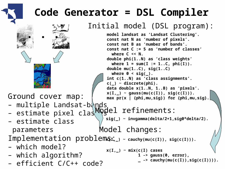
Code Generator = DSL Compiler
. . .
Ground cover map:– multiple Landsat-bands– estimate pixel classes– estimate class parametersImplementation problems:– which model?– which algorithm?– efficient C/C++ code?– correctness?
Generated program://----------------------------------------------------------------------------// Code file generated by AutoBayes V0.0.1// (c) 1999-2004 ASE Group, NASA Ames Research Center// Problem: Mixture of Gaussians// Source: examples/cover.ab// Command: ./autobayes// examples/cover.ab// Generated: Wed Mar 10 16:07:54 2004//----------------------------------------------------------------------------#include "autobayes.h"//----------------------------------------------------------------------------// Octave Function: cover//----------------------------------------------------------------------------DEFUN_DLD(cover,input_args,output_args, ""){ octave_value_list retval; if (input_args.length () != 4 || output_args != 3 ){ octave_stdout << "wrong usage"; return retval; } //-- Input declarations ---------------------------------------------------- // Number of classes octave_value arg_n_classes = input_args(0); if (!arg_n_classes.is_real_scalar()){ gripe_wrong_type_arg("n_classes", (const string &)"Scalar expected"); return retval; } double n_classes = (double)(arg_n_classes.double_value()); octave_value arg_x = input_args(1); if (!arg_x.is_real_matrix()){ gripe_wrong_type_arg("x", (const string &)"Matrix expected"); return retval; } Matrix x = (Matrix)(arg_x.matrix_value()); // Iteration tolerance for convergence loop octave_value arg_tolerance1 = input_args(2); if (!arg_tolerance1.is_real_scalar()){ gripe_wrong_type_arg("tolerance1", (const string &)"Scalar expected"); return retval; } double tolerance1 = (double)(arg_tolerance1.double_value()); // maximal number of EM iterations octave_value arg_maxiteration = input_args(3); if (!arg_maxiteration.is_real_scalar()){ gripe_wrong_type_arg("maxiteration", (const string &)"Scalar expected"); return retval; } double maxiteration = (double)(arg_maxiteration.double_value()); //-- Constant declarations ------------------------------------------------- // Number of data dimensions int n_dim = arg_x.rows(); // Number of data points int n_points = arg_x.columns(); // tolerance for appr. 600 data points double tolerance = 0.0003; //-- Output declarations --------------------------------------------------- Matrix mu(n_dim, n_classes); ColumnVector rho(n_classes); Matrix sigma(n_dim, n_classes); //-- Local declarations ---------------------------------------------------- // class assignment vector ColumnVector c(n_points); // Label: label0 // class membership table used in Discrete EM-algorithm Matrix q(n_points, n_classes); // local centers used for center-based initialization Matrix center(n_classes, n_dim); // Random index of data point int pick; // Loop variable int pv68; int pv65; int pv66; int pv42; int pv43; int pv13; int pv24; int pv56; int pv80; // Summation accumulator double pv83; double pv84; double pv85; // Lagrange-multiplier double l; // Common subexpression double pv52; // Memoized common subexpression ColumnVector pv58(n_classes); // Common subexpression double pv60; int pv70; int pv69; int pv71; Matrix muold(n_dim, n_classes); ColumnVector rhoold(n_classes); Matrix sigmaold(n_dim, n_classes); int pv73; int pv74; int pv75; int pv76; int pv77; // convergence loop counter int loopcounter; // sum up the Diffs double pv86; // Summation accumulator double pv92; double pv94; double pv95; double pv99; double pv98; double pv100; int pv26; int pv49; int pv48; int pv50; // Product accumulator double pv96; int pv53; int pv55; int pv89; int pv88; int pv87; int pv90; int pv91; // Check constraints on inputs ab_assert( 0 < n_classes ); ab_assert( 10 * n_classes < n_points ); ab_assert( 0 < n_dim ); ab_assert( 0 < n_points ); // Label: label1 // Label: label2 // Label: label4
// Discrete EM-algorithm // // The model describes a discrete latent (or hidden) variable problem with // the latent variable c and the data variable x. The problem to optimize // the conditional probability pr(x | {mu, rho, sigma}) w.r.t. the variables // mu, rho, and sigma can thus be solved by an application of the (discrete) // EM-algorithm. // The algorithm maintains as central data structure a class membership // table q (see "label0") such that q(pv13, pv61) is the probability that // data point pv13 belongs to class pv61, i.e., // q(pv13, pv61) == pr([c(pv13) == pv61]) // The algorithm consists of an initialization phase for q (see "label2"), // followed by a convergence phase (see "label5"). // // Initialization // The initialization is center-based, i.e., for each class (i.e., value of // the hidden variable c) a center value center is chosen first // (see "label4"). Then, the values for the local distribution are // calculated as distances between the data points and these center values // (see "label6"). // // Random initialization of the centers center with data points; // note that a data point can be picked as center more than once. for( pv65 = 0;pv65 <= n_classes - 1;pv65++ ) { pick = uniform_int_rnd(n_points - 1 - 0); for( pv66 = 0;pv66 <= n_dim - 1;pv66++ ) center(pv65, pv66) = x(pv66, pick); } // Label: label6 for( pv13 = 0;pv13 <= n_points - 1;pv13++ ) for( pv68 = 0;pv68 <= n_classes - 1;pv68++ ) { pv83 = 0; for( pv69 = 0;pv69 <= n_dim - 1;pv69++ ) pv83 += (center(pv68, pv69) - x(pv69, pv13)) * (center(pv68, pv69) - x(pv69, pv13)); pv85 = 0; for( pv70 = 0;pv70 <= n_classes - 1;pv70++ ) { pv84 = 0; for( pv71 = 0;pv71 <= n_dim - 1;pv71++ ) pv84 += (center(pv70, pv71) - x(pv71, pv13)) * (center(pv70, pv71) - x(pv71, pv13)); pv85 += sqrt(pv84); } q(pv13, pv68) = sqrt(pv83) / pv85; } // Label: label5 // EM-loop // // The EM-loop iterates two steps, expectation (or E-Step) (see "label7"), // and maximization (or M-Step) (see "label8"); however, due to the form of // the initialization used here, the are ordered the other way around. The // loop runs until convergence in the values of the variables mu, rho, and // sigma is achieved. loopcounter = 0; // repeat at least once pv86 = tolerance1; while( ((loopcounter < maxiteration) && (pv86 >= tolerance1)) ) { loopcounter = 1 + loopcounter; if ( loopcounter > 1 ) { // assign current values to old values for( pv73 = 0;pv73 <= n_dim - 1;pv73++ ) for( pv74 = 0;pv74 <= n_classes - 1;pv74++ ) muold(pv73, pv74) = mu(pv73, pv74); for( pv75 = 0;pv75 <= n_classes - 1;pv75++ ) rhoold(pv75) = rho(pv75); for( pv76 = 0;pv76 <= n_dim - 1;pv76++ ) for( pv77 = 0;pv77 <= n_classes - 1;pv77++ ) sigmaold(pv76, pv77) = sigma(pv76, pv77); } else ; // Label: label8 label3 // M-Step // // Decomposition I // The problem to optimize the conditional probability pr({c, x} | {mu, // rho, sigma}) w.r.t. the variables mu, rho, and sigma can under the // given dependencies by Bayes rule be decomposed into two independent // subproblems: // max pr(c | rho) for rho // max pr(x | {c, mu, sigma}) for {mu, sigma} // The conditional probability pr(c | rho) is under the dependencies // given in the model equivalent to // prod([pv17 := 0 .. n_points - 1], pr(c(pv17) | rho)) // The probability occuring here is atomic and can thus be replaced by // the respective probability density function given in the model. // Summing out the expected variable c(pv13) yields the log-likelihood // function // sum_domain([pv13 := 0 .. n_points - 1], // [pv18 := 0 .. n_classes - 1], [c(pv13)], q(pv13, pv18), // log(prod([pv17 := 0 .. n_points - 1], rho(c(pv17))))) // which can be simplified to // sum([pv18 := 0 .. n_classes - 1], // log(rho(pv18)) * sum([pv17 := 0 .. n_points - 1], q(pv17, pv18))) // This function is then optimized w.r.t. the goal variable rho. // The expression // sum([pv18 := 0 .. n_classes - 1], // log(rho(pv18)) * sum([pv17 := 0 .. n_points - 1], q(pv17, pv18))) // is maximized w.r.t. the variable rho under the constraint // 1 == sum([pv23 := 0 .. n_classes - 1], rho(pv23)) // using the Lagrange-multiplier l. l = n_points; for( pv24 = 0;pv24 <= n_classes - 1;pv24++ ) { // The summand // l // is constant with respect to the goal variable rho(pv24) and can // thus be ignored for maximization. The function // sum([pv18 := 0 .. n_classes - 1], // log(rho(pv18)) * // sum([pv17 := 0 .. n_points - 1], q(pv17, pv18))) - // l * sum([pv23 := 0 .. n_classes - 1], rho(pv23)) // is then symbolically maximized w.r.t. the goal variable rho(pv24). // The differential // sum([pv17 := 0 .. n_points - 1], q(pv17, pv24)) / rho(pv24) - l // is set to zero; this equation yields the solution // sum([pv26 := 0 .. n_points - 1], q(pv26, pv24)) / l pv92 = 0; for( pv26 = 0;pv26 <= n_points - 1;pv26++ ) pv92 += q(pv26, pv24); rho(pv24) = pv92 / l; } // The conditional probability pr(x | {c, mu, sigma}) is under the // dependencies given in the model equivalent to // prod([pv32 := 0 .. n_dim - 1, pv33 := 0 .. n_points - 1], // pr(x(pv32, pv33) | {c(pv33), mu(pv32, *), sigma(pv32, *)})) // The probability occuring here is atomic and can thus be replaced by // the respective probability density function given in the model. // Summing out the expected variable c(pv13) yields the log-likelihood // function // sum_domain([pv13 := 0 .. n_points - 1], // [pv34 := 0 .. n_classes - 1], [c(pv13)], q(pv13, pv34), // log(prod([pv32 := 0 .. n_dim - 1, // pv33 := 0 .. n_points - 1], // exp((x(pv32, pv33) - mu(pv32, c(pv33))) ** 2 / // -2 / sigma(pv32, c(pv33)) ** 2) / // (sqrt(2 * pi) * sigma(pv32, c(pv33))))))
// which can be simplified to // -((n_dim * n_points * (log(2) + log(pi)) + // sum([pv33 := 0 .. n_points - 1, pv34 := 0 .. n_classes - 1], // q(pv33, pv34) * // sum([pv32 := 0 .. n_dim - 1], // (x(pv32, pv33) - mu(pv32, pv34)) ** 2 / // sigma(pv32, pv34) ** 2))) / 2 + // sum([pv34 := 0 .. n_classes - 1], // sum([pv32 := 0 .. n_dim - 1], log(sigma(pv32, pv34))) * // sum([pv33 := 0 .. n_points - 1], q(pv33, pv34)))) // This function is then optimized w.r.t. the goal variables mu and // sigma. // The summands // n_dim * n_points * log(2) / -2 // n_dim * n_points * log(pi) / -2 // are constant with respect to the goal variables mu and sigma and can // thus be ignored for maximization. // Index decomposition // The function // -(sum([pv33 := 0 .. n_points - 1, pv34 := 0 .. n_classes - 1], // q(pv33, pv34) * // sum([pv32 := 0 .. n_dim - 1], // (x(pv32, pv33) - mu(pv32, pv34)) ** 2 / // sigma(pv32, pv34) ** 2)) / 2 + // sum([pv34 := 0 .. n_classes - 1], // sum([pv32 := 0 .. n_dim - 1], log(sigma(pv32, pv34))) * // sum([pv33 := 0 .. n_points - 1], q(pv33, pv34)))) // can be optimized w.r.t. the variables mu(pv42, pv43) and // sigma(pv42, pv43) element by element (i.e., along the index variables // pv42 and pv43) because there are no dependencies along thats dimensions. for( pv42 = 0;pv42 <= n_dim - 1;pv42++ ) for( pv43 = 0;pv43 <= n_classes - 1;pv43++ ) // The factors // n_classes // n_dim // are non-negative and constant with respect to the goal variables // mu(pv42, pv43) and sigma(pv42, pv43) and can thus be ignored for // maximization. // The function // -(log(sigma(pv42, pv43)) * // sum([pv33 := 0 .. n_points - 1], q(pv33, pv43)) + // sum([pv33 := 0 .. n_points - 1], // (x(pv42, pv33) - mu(pv42, pv43)) ** 2 * q(pv33, pv43)) / // (2 * sigma(pv42, pv43) ** 2)) // is then symbolically maximized w.r.t. the goal variables // mu(pv42, pv43) and sigma(pv42, pv43). The partial differentials // df / d_mu(pvar(42), pvar(43)) == // (sum([pv33 := 0 .. n_points - 1], // q(pv33, pv43) * x(pv42, pv33)) - // mu(pv42, pv43) * // sum([pv33 := 0 .. n_points - 1], q(pv33, pv43))) / // sigma(pv42, pv43) ** 2 // df / d_sigma(pvar(42), pvar(43)) == // sum([pv33 := 0 .. n_points - 1], // (x(pv42, pv33) - mu(pv42, pv43)) ** 2 * q(pv33, pv43)) / // sigma(pv42, pv43) ** 3 - // sum([pv33 := 0 .. n_points - 1], q(pv33, pv43)) / // sigma(pv42, pv43) // are set to zero; these equations yield the solutions // mu(pv42, pv43) == // cond(0 == sum([pv46 := 0 .. n_points - 1], q(pv46, pv43)), // fail(division_by_zero), // sum([pv48 := 0 .. n_points - 1], // q(pv48, pv43) * x(pv42, pv48)) / // sum([pv47 := 0 .. n_points - 1], q(pv47, pv43))) // sigma(pv42, pv43) == // cond(0 == sum([pv49 := 0 .. n_points - 1], q(pv49, pv43)), // fail(division_by_zero), // sqrt(sum([pv50 := 0 .. n_points - 1], // (x(pv42, pv50) - mu(pv42, pv43)) ** 2 * // q(pv50, pv43)) / // sum([pv51 := 0 .. n_points - 1], q(pv51, pv43)))) { // Initialization of common subexpression pv52 = 0; for( pv49 = 0;pv49 <= n_points - 1;pv49++ ) pv52 += q(pv49, pv43); if ( 0 == pv52 ) { ab_error( division_by_zero ); } else { pv94 = 0; for( pv48 = 0;pv48 <= n_points - 1;pv48++ ) pv94 += q(pv48, pv43) * x(pv42, pv48); mu(pv42, pv43) = pv94 / pv52; } if ( 0 == pv52 ) { ab_error( division_by_zero ); } else { pv95 = 0; for( pv50 = 0;pv50 <= n_points - 1;pv50++ ) pv95 += (x(pv42, pv50) - mu(pv42, pv43)) * (x(pv42, pv50) - mu(pv42, pv43)) * q(pv50, pv43); sigma(pv42, pv43) = sqrt(pv95 / pv52); } } // Label: label7 // E-Step // Update the current values of the class membership table q. for( pv13 = 0;pv13 <= n_points - 1;pv13++ ) { // Initialization of common subexpression for( pv56 = 0;pv56 <= n_classes - 1;pv56++ ) { pv96 = 1; for( pv53 = 0;pv53 <= n_dim - 1;pv53++ ) pv96 *= exp((x(pv53, pv13) - mu(pv53, pv56)) * (x(pv53, pv13) - mu(pv53, pv56)) / (double)(-2) / (sigma(pv53, pv56) * sigma(pv53, pv56))) / (sqrt(M_PI * (double)(2)) * sigma(pv53, pv56)); pv58(pv56) = pv96 * rho(pv56); } pv60 = 0; for( pv55 = 0;pv55 <= n_classes - 1;pv55++ ) pv60 += pv58(pv55); for( pv80 = 0;pv80 <= n_classes - 1;pv80++ ) // The denominator pv60 can become zero due to round-off errors. // In that case, each class is considered to be equally likely. if ( pv60 == 0 ) q(pv13, pv80) = (double)(1) / (double)(n_classes); else q(pv13, pv80) = pv58(pv80) / pv60; } if ( loopcounter > 1 ) { pv98 = 0; for( pv87 = 0;pv87 <= n_dim - 1;pv87++ ) for( pv88 = 0;pv88 <= n_classes - 1;pv88++ ) pv98 += abs(mu(pv87, pv88) - muold(pv87, pv88)) / (abs(mu(pv87, pv88)) + abs(muold(pv87, pv88))); pv99 = 0; for( pv89 = 0;pv89 <= n_classes - 1;pv89++ ) pv99 += abs(rho(pv89) - rhoold(pv89)) / (abs(rho(pv89)) + abs(rhoold(pv89))); pv100 = 0; for( pv90 = 0;pv90 <= n_dim - 1;pv90++ ) for( pv91 = 0;pv91 <= n_classes - 1;pv91++ ) pv100 += abs(sigma(pv90, pv91) - sigmaold(pv90, pv91)) / (abs(sigma(pv90, pv91)) + abs(sigmaold(pv90, pv91))); pv86 = pv98 + pv99 + pv100; } else ; } retval.resize(3); retval(0) = mu; retval(1) = rho; retval(2) = sigma; return retval;}//-- End of code ---------------------------------------------------------------
//----------------------------------------------------------------------------// Code file generated by AutoBayes V0.0.1// (c) 1999-2004 ASE Group, NASA Ames Research Center// Problem: Mixture of Gaussians// Source: examples/cover.ab// Command: ./autobayes// examples/cover.ab// Generated: Wed Mar 10 16:07:54 2004//----------------------------------------------------------------------------#include "autobayes.h"//----------------------------------------------------------------------------// Octave Function: cover//----------------------------------------------------------------------------DEFUN_DLD(cover,input_args,output_args, ""){ octave_value_list retval; if (input_args.length () != 4 || output_args != 3 ){ octave_stdout << "wrong usage"; return retval; } //-- Input declarations ---------------------------------------------------- // Number of classes octave_value arg_n_classes = input_args(0); if (!arg_n_classes.is_real_scalar()){ gripe_wrong_type_arg("n_classes", (const string &)"Scalar expected"); return retval; } double n_classes = (double)(arg_n_classes.double_value()); octave_value arg_x = input_args(1); if (!arg_x.is_real_matrix()){ gripe_wrong_type_arg("x", (const string &)"Matrix expected"); return retval; } Matrix x = (Matrix)(arg_x.matrix_value()); // Iteration tolerance for convergence loop octave_value arg_tolerance1 = input_args(2); if (!arg_tolerance1.is_real_scalar()){ gripe_wrong_type_arg("tolerance1", (const string &)"Scalar expected"); return retval; } double tolerance1 = (double)(arg_tolerance1.double_value()); // maximal number of EM iterations octave_value arg_maxiteration = input_args(3); if (!arg_maxiteration.is_real_scalar()){ gripe_wrong_type_arg("maxiteration", (const string &)"Scalar expected"); return retval; } double maxiteration = (double)(arg_maxiteration.double_value()); //-- Constant declarations ------------------------------------------------- // Number of data dimensions int n_dim = arg_x.rows(); // Number of data points int n_points = arg_x.columns(); // tolerance for appr. 600 data points double tolerance = 0.0003; //-- Output declarations --------------------------------------------------- Matrix mu(n_dim, n_classes); ColumnVector rho(n_classes); Matrix sigma(n_dim, n_classes); //-- Local declarations ---------------------------------------------------- // class assignment vector ColumnVector c(n_points); // Label: label0 // class membership table used in Discrete EM-algorithm Matrix q(n_points, n_classes); // local centers used for center-based initialization Matrix center(n_classes, n_dim); // Random index of data point int pick; // Loop variable int pv68; int pv65; int pv66; int pv42; int pv43; int pv13; int pv24; int pv56; int pv80; // Summation accumulator double pv83; double pv84; double pv85; // Lagrange-multiplier double l; // Common subexpression double pv52; // Memoized common subexpression ColumnVector pv58(n_classes); // Common subexpression double pv60; int pv70; int pv69; int pv71; Matrix muold(n_dim, n_classes); ColumnVector rhoold(n_classes); Matrix sigmaold(n_dim, n_classes); int pv73; int pv74; int pv75; int pv76; int pv77; // convergence loop counter int loopcounter; // sum up the Diffs double pv86; // Summation accumulator double pv92; double pv94; double pv95; double pv99; double pv98; double pv100; int pv26; int pv49; int pv48; int pv50; // Product accumulator double pv96; int pv53; int pv55; int pv89; int pv88; int pv87; int pv90; int pv91; // Check constraints on inputs ab_assert( 0 < n_classes ); ab_assert( 10 * n_classes < n_points ); ab_assert( 0 < n_dim ); ab_assert( 0 < n_points ); // Label: label1 // Label: label2 // Label: label4
// Discrete EM-algorithm // // The model describes a discrete latent (or hidden) variable problem with // the latent variable c and the data variable x. The problem to optimize // the conditional probability pr(x | {mu, rho, sigma}) w.r.t. the variables // mu, rho, and sigma can thus be solved by an application of the (discrete) // EM-algorithm. // The algorithm maintains as central data structure a class membership // table q (see "label0") such that q(pv13, pv61) is the probability that // data point pv13 belongs to class pv61, i.e., // q(pv13, pv61) == pr([c(pv13) == pv61]) // The algorithm consists of an initialization phase for q (see "label2"), // followed by a convergence phase (see "label5"). // // Initialization // The initialization is center-based, i.e., for each class (i.e., value of // the hidden variable c) a center value center is chosen first // (see "label4"). Then, the values for the local distribution are // calculated as distances between the data points and these center values // (see "label6"). // // Random initialization of the centers center with data points; // note that a data point can be picked as center more than once. for( pv65 = 0;pv65 <= n_classes - 1;pv65++ ) { pick = uniform_int_rnd(n_points - 1 - 0); for( pv66 = 0;pv66 <= n_dim - 1;pv66++ ) center(pv65, pv66) = x(pv66, pick); } // Label: label6 for( pv13 = 0;pv13 <= n_points - 1;pv13++ ) for( pv68 = 0;pv68 <= n_classes - 1;pv68++ ) { pv83 = 0; for( pv69 = 0;pv69 <= n_dim - 1;pv69++ ) pv83 += (center(pv68, pv69) - x(pv69, pv13)) * (center(pv68, pv69) - x(pv69, pv13)); pv85 = 0; for( pv70 = 0;pv70 <= n_classes - 1;pv70++ ) { pv84 = 0; for( pv71 = 0;pv71 <= n_dim - 1;pv71++ ) pv84 += (center(pv70, pv71) - x(pv71, pv13)) * (center(pv70, pv71) - x(pv71, pv13)); pv85 += sqrt(pv84); } q(pv13, pv68) = sqrt(pv83) / pv85; } // Label: label5 // EM-loop // // The EM-loop iterates two steps, expectation (or E-Step) (see "label7"), // and maximization (or M-Step) (see "label8"); however, due to the form of // the initialization used here, the are ordered the other way around. The // loop runs until convergence in the values of the variables mu, rho, and // sigma is achieved. loopcounter = 0; // repeat at least once pv86 = tolerance1; while( ((loopcounter < maxiteration) && (pv86 >= tolerance1)) ) { loopcounter = 1 + loopcounter; if ( loopcounter > 1 ) { // assign current values to old values for( pv73 = 0;pv73 <= n_dim - 1;pv73++ ) for( pv74 = 0;pv74 <= n_classes - 1;pv74++ ) muold(pv73, pv74) = mu(pv73, pv74); for( pv75 = 0;pv75 <= n_classes - 1;pv75++ ) rhoold(pv75) = rho(pv75); for( pv76 = 0;pv76 <= n_dim - 1;pv76++ ) for( pv77 = 0;pv77 <= n_classes - 1;pv77++ ) sigmaold(pv76, pv77) = sigma(pv76, pv77); } else ; // Label: label8 label3 // M-Step // // Decomposition I // The problem to optimize the conditional probability pr({c, x} | {mu, // rho, sigma}) w.r.t. the variables mu, rho, and sigma can under the // given dependencies by Bayes rule be decomposed into two independent // subproblems: // max pr(c | rho) for rho // max pr(x | {c, mu, sigma}) for {mu, sigma} // The conditional probability pr(c | rho) is under the dependencies // given in the model equivalent to // prod([pv17 := 0 .. n_points - 1], pr(c(pv17) | rho)) // The probability occuring here is atomic and can thus be replaced by // the respective probability density function given in the model. // Summing out the expected variable c(pv13) yields the log-likelihood // function // sum_domain([pv13 := 0 .. n_points - 1], // [pv18 := 0 .. n_classes - 1], [c(pv13)], q(pv13, pv18), // log(prod([pv17 := 0 .. n_points - 1], rho(c(pv17))))) // which can be simplified to // sum([pv18 := 0 .. n_classes - 1], // log(rho(pv18)) * sum([pv17 := 0 .. n_points - 1], q(pv17, pv18))) // This function is then optimized w.r.t. the goal variable rho. // The expression // sum([pv18 := 0 .. n_classes - 1], // log(rho(pv18)) * sum([pv17 := 0 .. n_points - 1], q(pv17, pv18))) // is maximized w.r.t. the variable rho under the constraint // 1 == sum([pv23 := 0 .. n_classes - 1], rho(pv23)) // using the Lagrange-multiplier l. l = n_points; for( pv24 = 0;pv24 <= n_classes - 1;pv24++ ) { // The summand // l // is constant with respect to the goal variable rho(pv24) and can // thus be ignored for maximization. The function // sum([pv18 := 0 .. n_classes - 1], // log(rho(pv18)) * // sum([pv17 := 0 .. n_points - 1], q(pv17, pv18))) - // l * sum([pv23 := 0 .. n_classes - 1], rho(pv23)) // is then symbolically maximized w.r.t. the goal variable rho(pv24). // The differential // sum([pv17 := 0 .. n_points - 1], q(pv17, pv24)) / rho(pv24) - l // is set to zero; this equation yields the solution // sum([pv26 := 0 .. n_points - 1], q(pv26, pv24)) / l pv92 = 0; for( pv26 = 0;pv26 <= n_points - 1;pv26++ ) pv92 += q(pv26, pv24); rho(pv24) = pv92 / l; } // The conditional probability pr(x | {c, mu, sigma}) is under the // dependencies given in the model equivalent to // prod([pv32 := 0 .. n_dim - 1, pv33 := 0 .. n_points - 1], // pr(x(pv32, pv33) | {c(pv33), mu(pv32, *), sigma(pv32, *)})) // The probability occuring here is atomic and can thus be replaced by // the respective probability density function given in the model. // Summing out the expected variable c(pv13) yields the log-likelihood // function // sum_domain([pv13 := 0 .. n_points - 1], // [pv34 := 0 .. n_classes - 1], [c(pv13)], q(pv13, pv34), // log(prod([pv32 := 0 .. n_dim - 1, // pv33 := 0 .. n_points - 1], // exp((x(pv32, pv33) - mu(pv32, c(pv33))) ** 2 / // -2 / sigma(pv32, c(pv33)) ** 2) / // (sqrt(2 * pi) * sigma(pv32, c(pv33))))))
// which can be simplified to // -((n_dim * n_points * (log(2) + log(pi)) + // sum([pv33 := 0 .. n_points - 1, pv34 := 0 .. n_classes - 1], // q(pv33, pv34) * // sum([pv32 := 0 .. n_dim - 1], // (x(pv32, pv33) - mu(pv32, pv34)) ** 2 / // sigma(pv32, pv34) ** 2))) / 2 + // sum([pv34 := 0 .. n_classes - 1], // sum([pv32 := 0 .. n_dim - 1], log(sigma(pv32, pv34))) * // sum([pv33 := 0 .. n_points - 1], q(pv33, pv34)))) // This function is then optimized w.r.t. the goal variables mu and // sigma. // The summands // n_dim * n_points * log(2) / -2 // n_dim * n_points * log(pi) / -2 // are constant with respect to the goal variables mu and sigma and can // thus be ignored for maximization. // Index decomposition // The function // -(sum([pv33 := 0 .. n_points - 1, pv34 := 0 .. n_classes - 1], // q(pv33, pv34) * // sum([pv32 := 0 .. n_dim - 1], // (x(pv32, pv33) - mu(pv32, pv34)) ** 2 / // sigma(pv32, pv34) ** 2)) / 2 + // sum([pv34 := 0 .. n_classes - 1], // sum([pv32 := 0 .. n_dim - 1], log(sigma(pv32, pv34))) * // sum([pv33 := 0 .. n_points - 1], q(pv33, pv34)))) // can be optimized w.r.t. the variables mu(pv42, pv43) and // sigma(pv42, pv43) element by element (i.e., along the index variables // pv42 and pv43) because there are no dependencies along thats dimensions. for( pv42 = 0;pv42 <= n_dim - 1;pv42++ ) for( pv43 = 0;pv43 <= n_classes - 1;pv43++ ) // The factors // n_classes // n_dim // are non-negative and constant with respect to the goal variables // mu(pv42, pv43) and sigma(pv42, pv43) and can thus be ignored for // maximization. // The function // -(log(sigma(pv42, pv43)) * // sum([pv33 := 0 .. n_points - 1], q(pv33, pv43)) + // sum([pv33 := 0 .. n_points - 1], // (x(pv42, pv33) - mu(pv42, pv43)) ** 2 * q(pv33, pv43)) / // (2 * sigma(pv42, pv43) ** 2)) // is then symbolically maximized w.r.t. the goal variables // mu(pv42, pv43) and sigma(pv42, pv43). The partial differentials // df / d_mu(pvar(42), pvar(43)) == // (sum([pv33 := 0 .. n_points - 1], // q(pv33, pv43) * x(pv42, pv33)) - // mu(pv42, pv43) * // sum([pv33 := 0 .. n_points - 1], q(pv33, pv43))) / // sigma(pv42, pv43) ** 2 // df / d_sigma(pvar(42), pvar(43)) == // sum([pv33 := 0 .. n_points - 1], // (x(pv42, pv33) - mu(pv42, pv43)) ** 2 * q(pv33, pv43)) / // sigma(pv42, pv43) ** 3 - // sum([pv33 := 0 .. n_points - 1], q(pv33, pv43)) / // sigma(pv42, pv43) // are set to zero; these equations yield the solutions // mu(pv42, pv43) == // cond(0 == sum([pv46 := 0 .. n_points - 1], q(pv46, pv43)), // fail(division_by_zero), // sum([pv48 := 0 .. n_points - 1], // q(pv48, pv43) * x(pv42, pv48)) / // sum([pv47 := 0 .. n_points - 1], q(pv47, pv43))) // sigma(pv42, pv43) == // cond(0 == sum([pv49 := 0 .. n_points - 1], q(pv49, pv43)), // fail(division_by_zero), // sqrt(sum([pv50 := 0 .. n_points - 1], // (x(pv42, pv50) - mu(pv42, pv43)) ** 2 * // q(pv50, pv43)) / // sum([pv51 := 0 .. n_points - 1], q(pv51, pv43)))) { // Initialization of common subexpression pv52 = 0; for( pv49 = 0;pv49 <= n_points - 1;pv49++ ) pv52 += q(pv49, pv43); if ( 0 == pv52 ) { ab_error( division_by_zero ); } else { pv94 = 0; for( pv48 = 0;pv48 <= n_points - 1;pv48++ ) pv94 += q(pv48, pv43) * x(pv42, pv48); mu(pv42, pv43) = pv94 / pv52; } if ( 0 == pv52 ) { ab_error( division_by_zero ); } else { pv95 = 0; for( pv50 = 0;pv50 <= n_points - 1;pv50++ ) pv95 += (x(pv42, pv50) - mu(pv42, pv43)) * (x(pv42, pv50) - mu(pv42, pv43)) * q(pv50, pv43); sigma(pv42, pv43) = sqrt(pv95 / pv52); } } // Label: label7 // E-Step // Update the current values of the class membership table q. for( pv13 = 0;pv13 <= n_points - 1;pv13++ ) { // Initialization of common subexpression for( pv56 = 0;pv56 <= n_classes - 1;pv56++ ) { pv96 = 1; for( pv53 = 0;pv53 <= n_dim - 1;pv53++ ) pv96 *= exp((x(pv53, pv13) - mu(pv53, pv56)) * (x(pv53, pv13) - mu(pv53, pv56)) / (double)(-2) / (sigma(pv53, pv56) * sigma(pv53, pv56))) / (sqrt(M_PI * (double)(2)) * sigma(pv53, pv56)); pv58(pv56) = pv96 * rho(pv56); } pv60 = 0; for( pv55 = 0;pv55 <= n_classes - 1;pv55++ ) pv60 += pv58(pv55); for( pv80 = 0;pv80 <= n_classes - 1;pv80++ ) // The denominator pv60 can become zero due to round-off errors. // In that case, each class is considered to be equally likely. if ( pv60 == 0 ) q(pv13, pv80) = (double)(1) / (double)(n_classes); else q(pv13, pv80) = pv58(pv80) / pv60; } if ( loopcounter > 1 ) { pv98 = 0; for( pv87 = 0;pv87 <= n_dim - 1;pv87++ ) for( pv88 = 0;pv88 <= n_classes - 1;pv88++ ) pv98 += abs(mu(pv87, pv88) - muold(pv87, pv88)) / (abs(mu(pv87, pv88)) + abs(muold(pv87, pv88))); pv99 = 0; for( pv89 = 0;pv89 <= n_classes - 1;pv89++ ) pv99 += abs(rho(pv89) - rhoold(pv89)) / (abs(rho(pv89)) + abs(rhoold(pv89))); pv100 = 0; for( pv90 = 0;pv90 <= n_dim - 1;pv90++ ) for( pv91 = 0;pv91 <= n_classes - 1;pv91++ ) pv100 += abs(sigma(pv90, pv91) - sigmaold(pv90, pv91)) / (abs(sigma(pv90, pv91)) + abs(sigmaold(pv90, pv91))); pv86 = pv98 + pv99 + pv100; } else ; } retval.resize(3); retval(0) = mu; retval(1) = rho; retval(2) = sigma; return retval;}//-- End of code ---------------------------------------------------------------
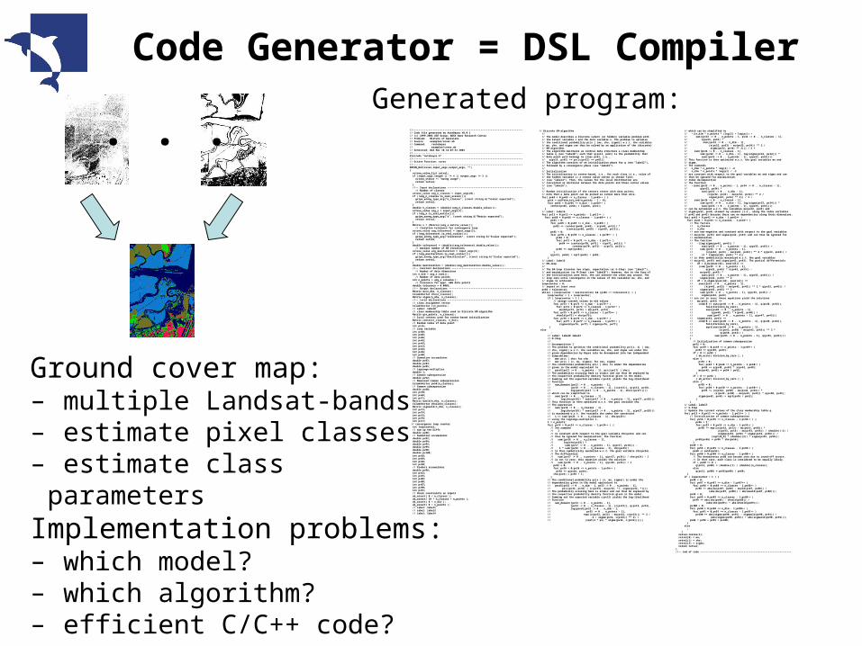
Code Generator = DSL Compiler
. . .
Ground cover map:– multiple Landsat-bands– estimate pixel classes– estimate class parametersImplementation problems:– which model?– which algorithm?– efficient C/C++ code?– correctness?
Generated program:• ~ 1sec. generation time• ≥ 600 lines• ≥ 1:30 leverage• fully documented• deeply nested loops• complex calculations• “correct-by-construction”
Generator Assurance
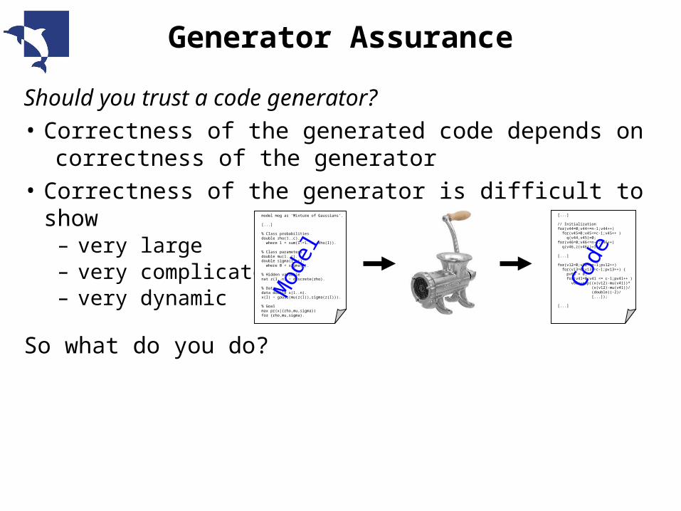
Should you trust a code generator?• Correctness of the generated code depends on
correctness of the generator• Correctness of the generator is difficult to show
– very large– very complicated– very dynamic
So what do you do?
model mog as 'Mixture of Gaussians'.
[...]
% Class probabilitiesdouble rho(1..c). where 1 = sum(I:=1..c, rho(I)).
% Class parametersdouble mu(1..c).double sigma(1..c). where 0 < sigma(_).
% Hidden variablenat z(1..n) ~ discrete(rho).
% Datadata double x(1..n).x(I) ~ gauss(mu(z(I)),sigma(z(I))).
% Goalmax pr(x|{rho,mu,sigma})for {rho,mu,sigma}.
[...]
// Initializationfor(v44=0;v44<=n-1;v44++) for(v45=0;v45<=c-1;v45++ ) q(v44,v45)=0;for(v46=0;v46<=n-1;v46++) q(v46,z(v46))=1;
[...]
for(v12=0;v12<=n-1;pv12++) for(v13=0;v13<=c-1;pv13++) { pv68 = 0; for(v41=0;v41 <= c-1;pv41++ ) v68+=exp((x(v12)-mu(v41))* (x(v12)-mu(v41))/ (double)(-2)/ [...]); [...]
Mod
el
Cod
e
Generator Assurance
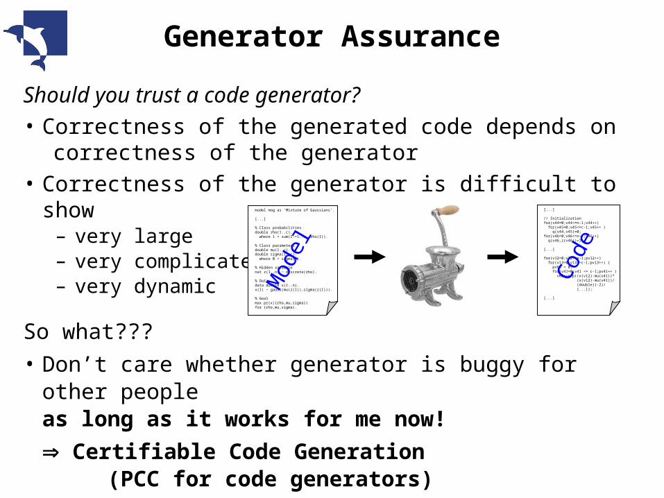
Should you trust a code generator?• Correctness of the generated code depends on
correctness of the generator• Correctness of the generator is difficult to show
– very large– very complicated– very dynamic
So what???
• Don’t care whether generator is buggy for other peopleas long as it works for me now!
Certifiable Code Generation (PCC for code generators)
model mog as 'Mixture of Gaussians'.
[...]
% Class probabilitiesdouble rho(1..c). where 1 = sum(I:=1..c, rho(I)).
% Class parametersdouble mu(1..c).double sigma(1..c). where 0 < sigma(_).
% Hidden variablenat z(1..n) ~ discrete(rho).
% Datadata double x(1..n).x(I) ~ gauss(mu(z(I)),sigma(z(I))).
% Goalmax pr(x|{rho,mu,sigma})for {rho,mu,sigma}.
[...]
// Initializationfor(v44=0;v44<=n-1;v44++) for(v45=0;v45<=c-1;v45++ ) q(v44,v45)=0;for(v46=0;v46<=n-1;v46++) q(v46,z(v46))=1;
[...]
for(v12=0;v12<=n-1;pv12++) for(v13=0;v13<=c-1;pv13++) { pv68 = 0; for(v41=0;v41 <= c-1;pv41++ ) v68+=exp((x(v12)-mu(v41))* (x(v12)-mu(v41))/ (double)(-2)/ [...]); [...]
Mod
el
Cod
e
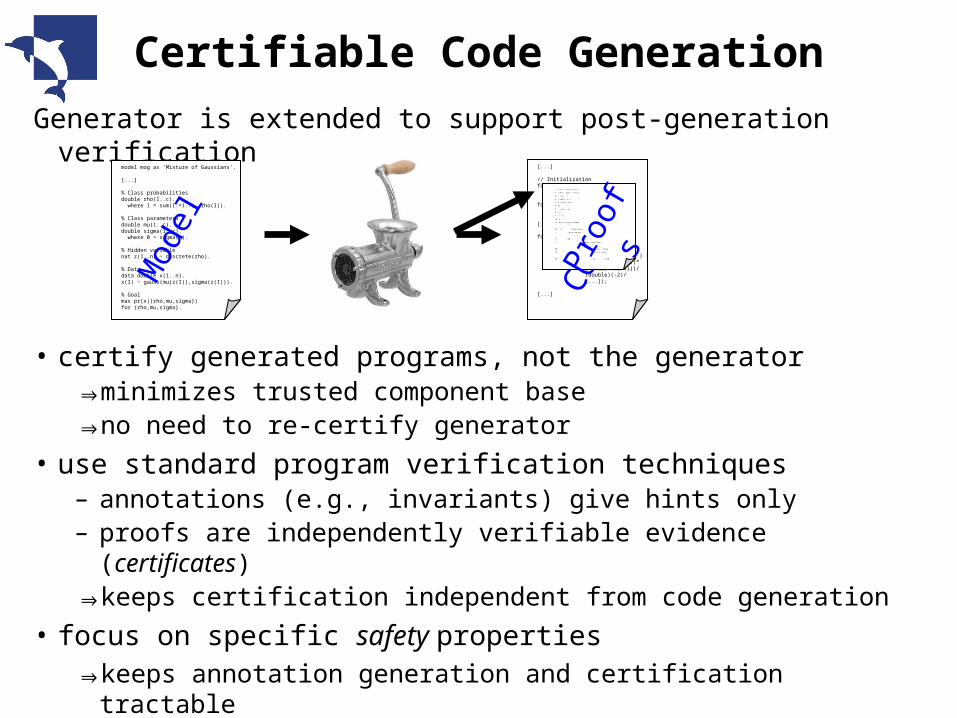
Generator is extended to support post-generation verification
• certify generated programs, not the generator⇒ minimizes trusted component base⇒ no need to re-certify generator
• use standard program verification techniques– annotations (e.g., invariants) give hints only– proofs are independently verifiable evidence (certificates)⇒ keeps certification independent from code generation
• focus on specific safety properties ⇒ keeps annotation generation and certification tractable
Certifiable Code Generation
model mog as 'Mixture of Gaussians'.
[...]
% Class probabilitiesdouble rho(1..c). where 1 = sum(I:=1..c, rho(I)).
% Class parametersdouble mu(1..c).double sigma(1..c). where 0 < sigma(_).
% Hidden variablenat z(1..n) ~ discrete(rho).
% Datadata double x(1..n).x(I) ~ gauss(mu(z(I)),sigma(z(I))).
% Goalmax pr(x|{rho,mu,sigma})for {rho,mu,sigma}.
[...]
// Initializationfor(v44=0;v44<=n-1;v44++) for(v45=0;v45<=c-1;v45++ ) q(v44,v45)=0;for(v46=0;v46<=n-1;v46++) q(v46,z(v46))=1;
[...]
for(v12=0;v12<=n-1;pv12++) for(v13=0;v13<=c-1;pv13++) { pv68 = 0; for(v41=0;v41 <= c-1;pv41++ ) v68+=exp((x(v12)-mu(v41))* (x(v12)-mu(v41))/ (double)(-2)/ [...]); [...]
Mod
el
Cod
eP
roof
s

Hoare-Style Certification Framework
Safety property: formal characterization of aspects of intuitively
safe programs– introduce “shadow variables” to record safety information
– extend operational semantics by effects on shadow variables
– define semantic safety judgements on expressions/statements
Safety policy: proof rules designed to show that safety property
holds for program– extend Hoare-rules by safety predicate and shadow variables
⇒ prove soundness and completeness (offline, manual)
Safety Properties
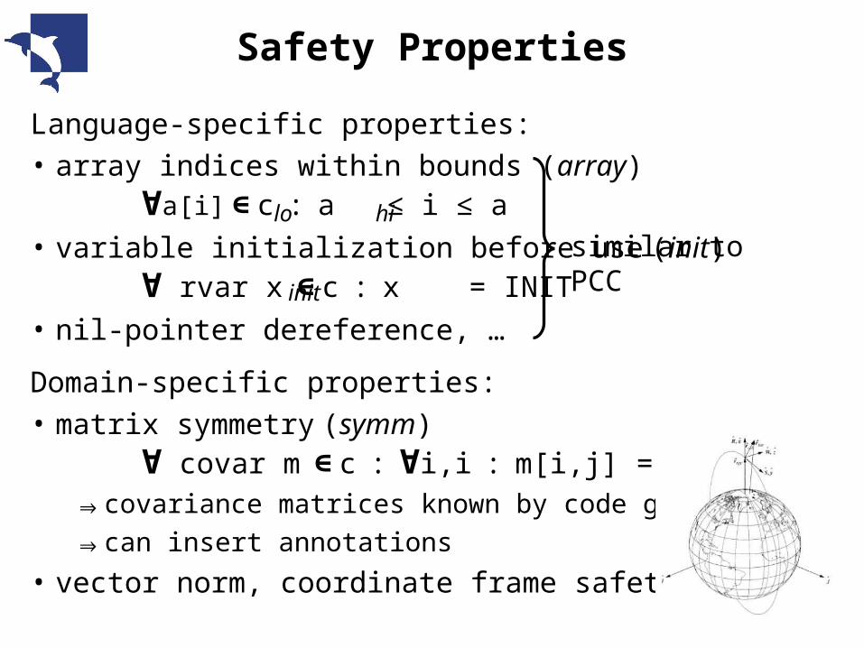
Language-specific properties:• array indices within bounds (array)
∀a[i] ∈ c : a ≤ i ≤ a• variable initialization before use (init)
∀ rvar x ∈ c : x = INIT• nil-pointer dereference, …
Domain-specific properties:• matrix symmetry (symm)
∀ covar m ∈ c : ∀i,i : m[i,j] = m[j,i] ⇒ covariance matrices known by code generator⇒ can insert annotations
• vector norm, coordinate frame safety, …
init
lo hi
similar to PCC

Certification Architecture
• standard PCC architecture• “organically grown” job control:
– run scripts based on SystemOnTPTP
– dynamic axiom generation (sed / awk)
– dynamic axiom selection (based on problem names)

Lessons
Lesson #1: Things don’t go wrong in the ATP
Most errors are in the application, axiomatization, or integration:• interface between application and ATP == proof task
– application debugging == task proving / refuting⇒ application errors difficult to detect
• application must provide full axiomatization (axioms / lemmas)– no standards ⇒ no reuse– consistency difficult to ensure manually
• integration needs generally supported job control language– better than SystemOnTPTP + shell scripts + C pre-processor
⇒applications need more robust ATPs– better error checking: free variables, ill-sorted terms, …– consistency checking more important than proof checking
Lesson #2: TPTP ≠ Real World
Applications and benchmarks have different profiles• full (typed) FOF vs. CNF, UEQ, HNE, EPR, …
– clausification is integral part of ATP
– problems in subclasses are rare (almost accidental)⇒ ATPs need to work on full FOF
(⇒ branch to specialized solvers hidden)
• task stream vs. single task: one problem = many tasks– success only if all tasks proven
– most tasks relatively simple, but often large
– most problems contain hard tasks
– background theory remains stable⇒ ATPs need to minimize overhead (⇒ batch mode)⇒ATPs should be easily tunable to application domain
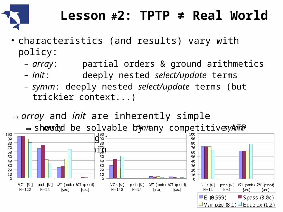
Lesson #2: TPTP ≠ Real World
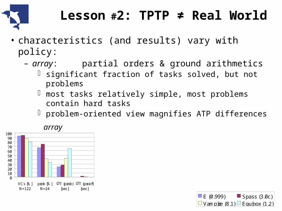
• characteristics (and results) vary with policy:– array: partial orders & ground arithmetics
significant fraction of tasks solved, but not problems most tasks relatively simple, most problems contain hard tasks problem-oriented view magnifies ATP differences
E (0.999) Spass (3.0c)Vampire (8.1) Equinox (1.2)
array
0102030405060708090
100
VCs [%]N=122
prob [%]N=24
∅T (prob)[sec]
∅T (proof)[sec]

Lesson #2: TPTP ≠ Real World
• characteristics (and results) vary with policy:– array: partial orders & ground arithmetics– init: deeply nested select/update terms
completely overwhelms ATPs response times determined by Tmax (60secs.)
E (0.999) Spass (3.0c)Vampire (8.1) Equinox (1.2)
array init
0102030405060708090
100
VCs [%]N=122
prob [%]N=24
∅T (prob)[sec]
∅T (proof)[sec]
0102030405060708090
100
VCs [%]N=140
prob [%]N=24
∅T (prob)[min]
∅T (proof)[sec]
Lesson #2: TPTP ≠ Real World
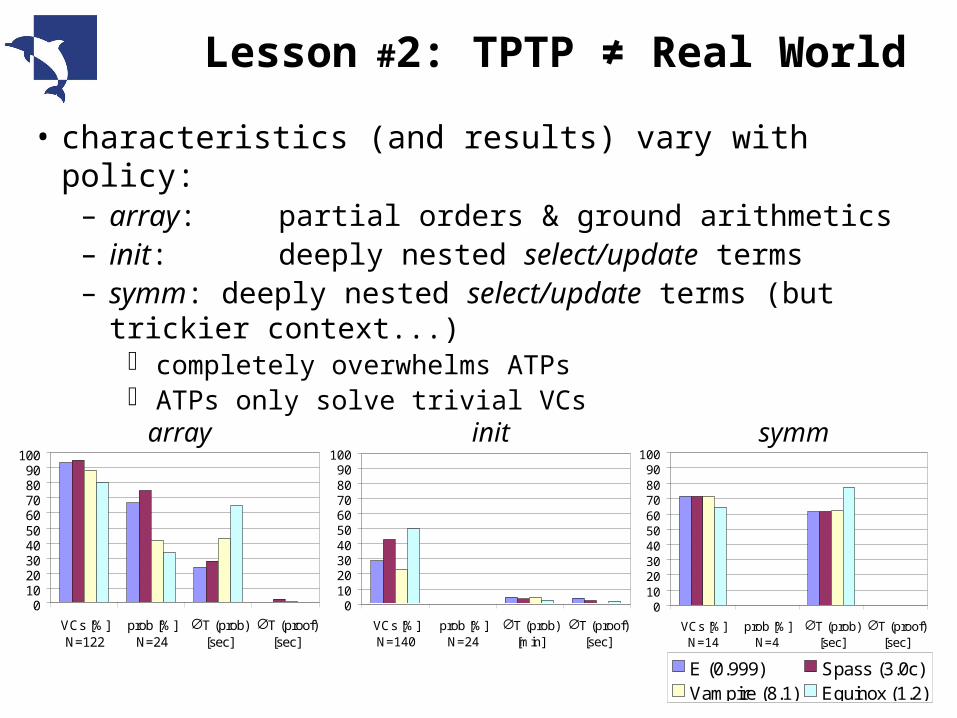
• characteristics (and results) vary with policy:– array: partial orders & ground arithmetics– init: deeply nested select/update terms– symm: deeply nested select/update terms (but trickier context...)
completely overwhelms ATPs ATPs only solve trivial VCs
E (0.999) Spass (3.0c)Vampire (8.1) Equinox (1.2)
0102030405060708090
100
VCs [%]N=14
prob [%]N=4
∅T (prob)[sec]
∅T (proof)[sec]
array init
0102030405060708090
100
VCs [%]N=122
prob [%]N=24
∅T (prob)[sec]
∅T (proof)[sec]
0102030405060708090
100
VCs [%]N=140
prob [%]N=24
∅T (prob)[min]
∅T (proof)[sec]
symm
E (0.999) Spass (3.0c)Vampire (8.1) Equinox (1.2)
0102030405060708090
100
VCs [%]N=14
prob [%]N=4
∅T (prob)[sec]
∅T (proof)[sec]
Lesson #2: TPTP ≠ Real World
array init
• characteristics (and results) vary with policy:– array: partial orders & ground arithmetics– init: deeply nested select/update terms– symm: deeply nested select/update terms (but trickier context...)
⇒array and init are inherently simple⇒ should be solvable by any competitive ATP (“low-hanging fruit”)⇒ TPTP overtuning?
0102030405060708090
100
VCs [%]N=122
prob [%]N=24
∅T (prob)[sec]
∅T (proof)[sec]
0102030405060708090
100
VCs [%]N=140
prob [%]N=24
∅T (prob)[min]
∅T (proof)[sec]
symm
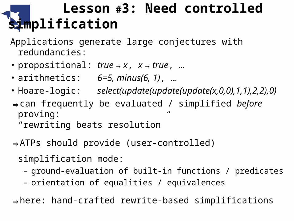
Lesson #3: Need controlled simplification
Applications generate large conjectures with redundancies:• propositional: true → x, x → true, …• arithmetics: 6=5, minus(6, 1), …• Hoare-logic:
select(update(update(update(x,0,0),1,1),2,2),0)⇒can frequently be evaluated / simplified before proving:
“rewriting beats resolution”
⇒ATPs should provide (user-controlled) simplification mode:– ground-evaluation of built-in functions / predicates
– orientation of equalities / equivalences
⇒here: hand-crafted rewrite-based simplifications
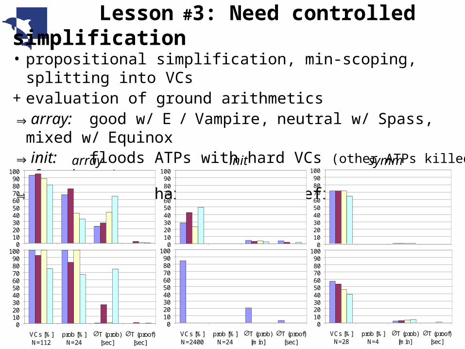
• propositional simplification, min-scoping, splitting into VCs+ evaluation of ground arithmetics⇒array: good w/ E / Vampire, neutral w/ Spass, mixed w/
Equinox⇒init: floods ATPs with hard VCs (other ATPs killed after hours)
⇒symm: splits hard VCs, no benefits
0102030405060708090
100
VCs [%]N=14
prob [%]N=4
∅T (prob)[min]
∅T (proof)[sec]
array init
0102030405060708090
100
VCs [%]N=122
prob [%]N=24
∅T (prob)[sec]
∅T (proof)[sec]
0102030405060708090
100
VCs [%]N=140
prob [%]N=24
∅T (prob)[min]
∅T (proof)[sec]
symm
Lesson #3: Need controlled simplification
0102030405060708090
100
VCs [%]N=112
prob [%]N=24
∅T (prob)[sec]
∅T (proof)[sec]
0102030405060708090
100
VCs [%]N=2400
prob [%]N=24
∅T (prob)[min]
∅T (proof)[sec]
0102030405060708090
100
VCs [%]N=28
prob [%]N=4
∅T (prob)[min]
∅T (proof)[sec]
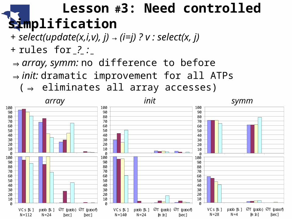
+ select(update(x,i,v), j) → (i=j) ? v : select(x, j)+ rules for _?_ : _⇒array, symm: no difference to before⇒init: dramatic improvement for all ATPs
( eliminates all array accesses)⇒
0102030405060708090
100
VCs [%]N=14
prob [%]N=4
∅T (prob)[sec]
∅T (proof)[sec]
array init
0102030405060708090
100
VCs [%]N=122
prob [%]N=24
∅T (prob)[sec]
∅T (proof)[sec]
0102030405060708090
100
VCs [%]N=140
prob [%]N=24
∅T (prob)[min]
∅T (proof)[sec]
symm
Lesson #3: Need controlled simplification
0102030405060708090
100
VCs [%]N=112
prob [%]N=24
∅T (prob)[sec]
∅T (proof)[sec]
0102030405060708090
100
VCs [%]N=140
prob [%]N=24
∅T (prob)[min]
∅T (proof)[sec]
0102030405060708090
100
VCs [%]N=28
prob [%]N=4
∅T (prob)[min]
∅T (proof)[sec]
0102030405060708090
100
VCs [%]N=14
prob [%]N=4
∅T (prob)[sec]
∅T (proof)[sec]
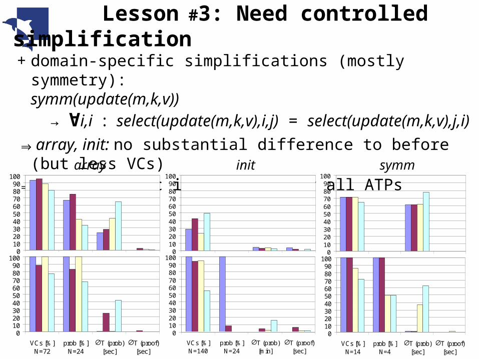
+ domain-specific simplifications (mostly symmetry):symm(update(m,k,v)) → ∀i,i : select(update(m,k,v),i,j) = select(update(m,k,v),j,i)
⇒array, init: no substantial difference to before (but less VCs)⇒symm: dramatic improvement for all ATPs
array init
0102030405060708090
100
VCs [%]N=122
prob [%]N=24
∅T (prob)[sec]
∅T (proof)[sec]
0102030405060708090
100
VCs [%]N=140
prob [%]N=24
∅T (prob)[min]
∅T (proof)[sec]
symm
Lesson #3: Need controlled simplification
0102030405060708090
100
VCs [%]N=72
prob [%]N=24
∅T (prob)[sec]
∅T (proof)[sec]
0102030405060708090
100
VCs [%]N=140
prob [%]N=24
∅T (prob)[min]
∅T (proof)[sec]
0102030405060708090
100
VCs [%]N=14
prob [%]N=4
∅T (prob)[sec]
∅T (proof)[sec]
Lesson #4: Need axiom selection
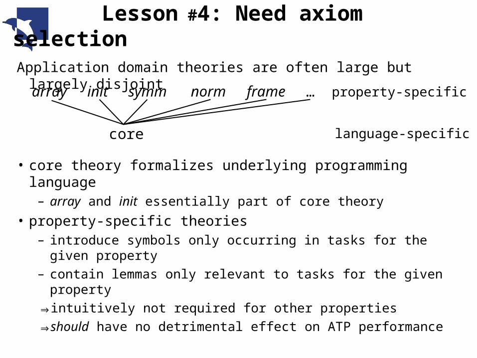
Application domain theories are often large but largely disjoint
• core theory formalizes underlying programming language– array and init essentially part of core theory
• property-specific theories – introduce symbols only occurring in tasks for the given property
– contain lemmas only relevant to tasks for the given property⇒ intuitively not required for other properties⇒ should have no detrimental effect on ATP performance
core
array init symm norm frame … property-specific
language-specific

Lesson #4: Need axiom selection
E (0.999) Spass (3.0c)Vampire (8.1) Equinox (1.2)
init init + exp. symm init + imp. symm
0102030405060708090
100
VCs [%]N=782
prob [%]N=24
∅T (prob)[min]
∅T (proof)[sec]
0102030405060708090
100
VCs [%]N=782
prob [%]N=24
∅T (prob)[min]
∅T (proof)[sec]
0102030405060708090
100
VCs [%]N=782
prob [%]N=24
∅T (prob)[min]
∅T (proof)[sec]
Example: init with redundant symm-axioms:• explicit symmetry-predicate:
∀i,i : select(m,i,j) = select(m,j,i) ⇒ symm(m)symm(n) ∧ symm(m) ⇒ symm(madd(n, m))
• implicit symmetry: ∀i,i : select(n,i,j) = select(n,j,i) ∧select(m,i,j) =
select(m,j,i) ⇒ select(madd(n,m),i,j) = select(madd(n,m),j,i)
Lesson #4: Need axiom selection
⇒ATPs shouldn’t flatten structure in the domain theory– similar to distinction conjecture vs. axioms
– coarse selection based on file structuring can be controlled by application
– detailed selection based on signature of conjecture might be benificial (cf. Reif / Schellhorn 1998)
Lesson #5: Need built-in theory support
Applications use the same domain theories over and over again:• “It's disgraceful that we have to define integers using succ's,
and make up our own array syntax“– significant engineering effort– no standards ⇒ no reuse
• hand-crafted axiomatizations are…– typically incomplete– typically sub-optimal for ATP– typically need generators to handle occurring literals
can add 3=succ(succ(succ(0))) but what about 1023? shell scripts generate axioms for
– Pressburgerization, finite domains (small numbers only)
– ground orders (gt/leq), ground arithmetic (all occurring numbers)
– often inadequate (i.e., wrong)– often inconsistent

Lesson #5: Need built-in theory support
FOL ATPs should “steal” from SMT-LIB and HO systems and
provide libraries of standard theories:• TPTP TFF (typed FOL and built-in arithmetics) is a good start
⇒ Your ATP should support that!
• SMT-LIB is a good goal to aim for• theories can be implemented by
– axiom generation
– decision procedures⇒ Your ATP should support that!
Lesson #6: Need ATP Plug&Play
No single off-the-shelf ATP is optimal for all problems• combine ATPs with different preprocessing steps
– clausification
– simplification
– axiom selection
• ATP combinators– sequential composition
– parallel competition
– …
⇒TPTPWorld is a good ATP harness but not a gluing framework
Conclusions
• (Software engineering) applications are tractable– no fancy logic, just POFOL and normal theories
– different characteristics than TPTP (except for SWC and SWV :-)
• Support theories!– theory libraries, built-in symbols
– light-weight support sufficient
• ATP customization– exploit regularities from application
– user-controlled pre-processing⇒ grab low-hanging fruits!
• Success = Proof and Integration – need robust tools
– need Plug&Play framework