Bernhard Steinberger

Deutsches GeoForschungsZentrum, Potsdam and

Centre for Earth Evolution and Dynamics, Univ. Oslo

Geodynamic relations between subduction, plume generation,LLSVPs and true polar wander

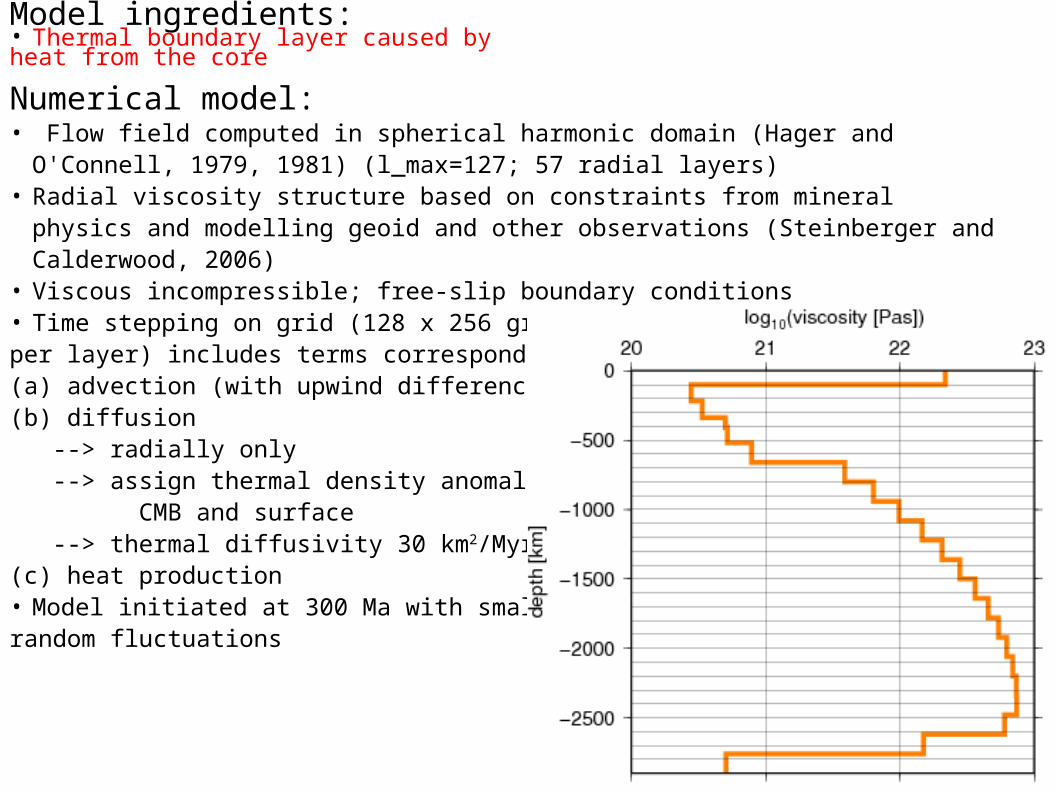
Model ingredients:• Thermal boundary layer caused by heat from the core

Numerical model:• Flow field computed in spherical harmonic domain (Hager and O'Connell, 1979,

1981) (l_max=127; 57 radial layers)• Radial viscosity structure based on constraints from mineral physics and

modelling geoid and other observations (Steinberger and Calderwood, 2006)• Viscous incompressible; free-slip boundary conditions• Time stepping on grid (128 x 256 grid points per layer) includes terms corresponding to(a) advection (with upwind differencing scheme)(b) diffusion --> radially only --> assign thermal density anomaly at CMB and surface --> thermal diffusivity 30 km2/Myr(c) heat production• Model initiated at 300 Ma with small random fluctuations

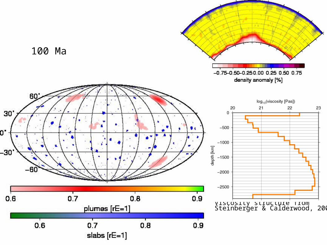
100 Ma

Viscosity structure fromSteinberger & Calderwood, 2006

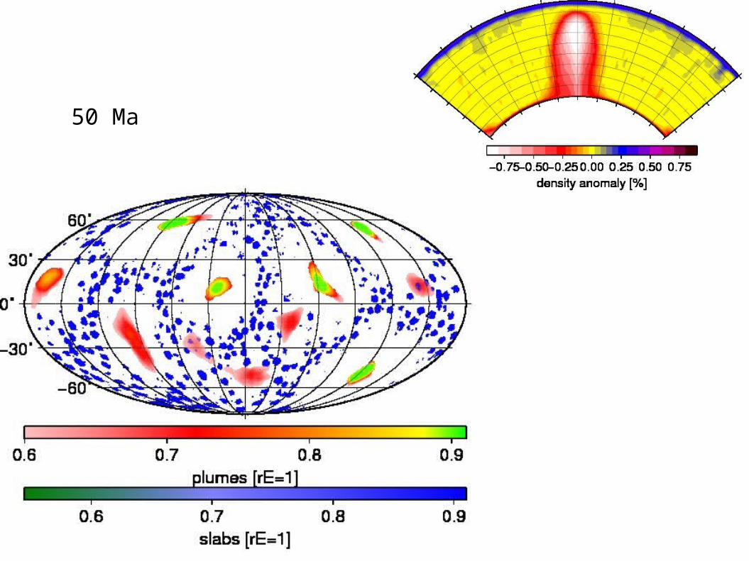
50 Ma

0 Ma

Plumes rather stableRelevance for Venus?Application to specific hotspots with seeding at specific locations

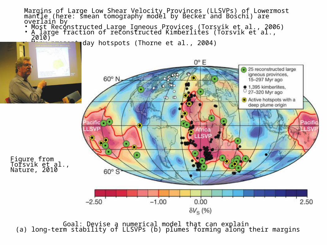
Margins of Large Low Shear Velocity Provinces (LLSVPs) of Lowermost mantle (here: smean tomography model by Becker and Boschi) are overlain by• Most Reconstructed Large Igneous Provices (Torsvik et al., 2006)• A large fraction of reconstructed Kimberlites (Torsvik et al., 2010)• Many present-day hotspots (Thorne et al., 2004)

Figure from Torsvik et al., Nature, 2010

Goal: Devise a numerical model that can explain (a) long-term stability of LLSVPs (b) plumes forming along their margins

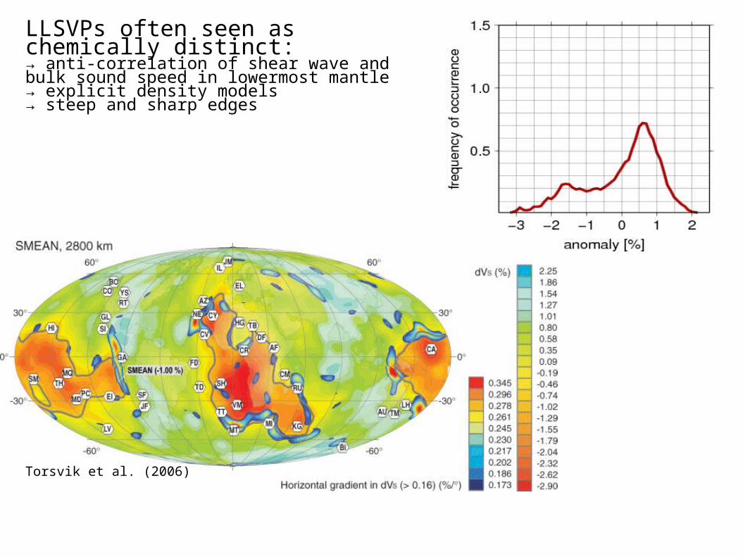
Torsvik et al. (2006)

LLSVPs often seen as chemically distinct:→ anti-correlation of shear wave and bulk sound speed in lowermost mantle→ explicit density models→ steep and sharp edges

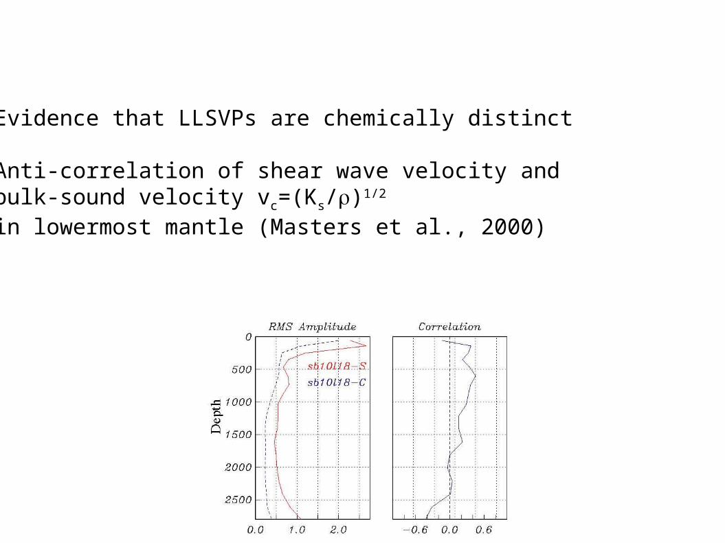
Evidence that LLSVPs are chemically distinct

Anti-correlation of shear wave velocity andbulk-sound velocity vc=(Ks/r)1/2

in lowermost mantle (Masters et al., 2000)

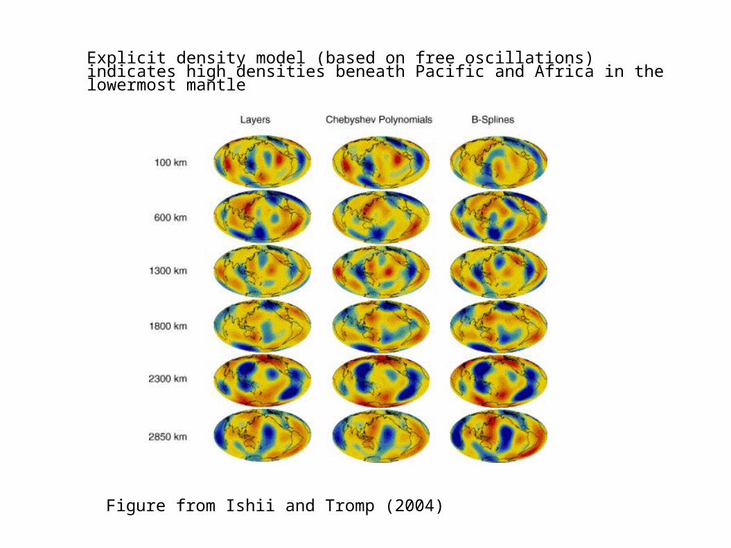
Explicit density model (based on free oscillations) indicates high densities beneath Pacific and Africa in the lowermost mantle

Figure from Ishii and Tromp (2004)

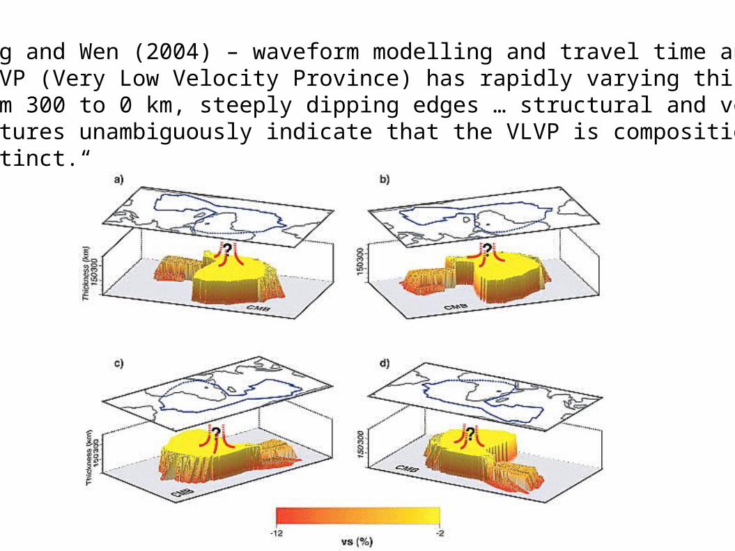
Wang and Wen (2004) – waveform modelling and travel time analysis„VLVP (Very Low Velocity Province) has rapidly varying thicknessesfrom 300 to 0 km, steeply dipping edges … structural and velocityfeatures unambiguously indicate that the VLVP is compositionallydistinct.“

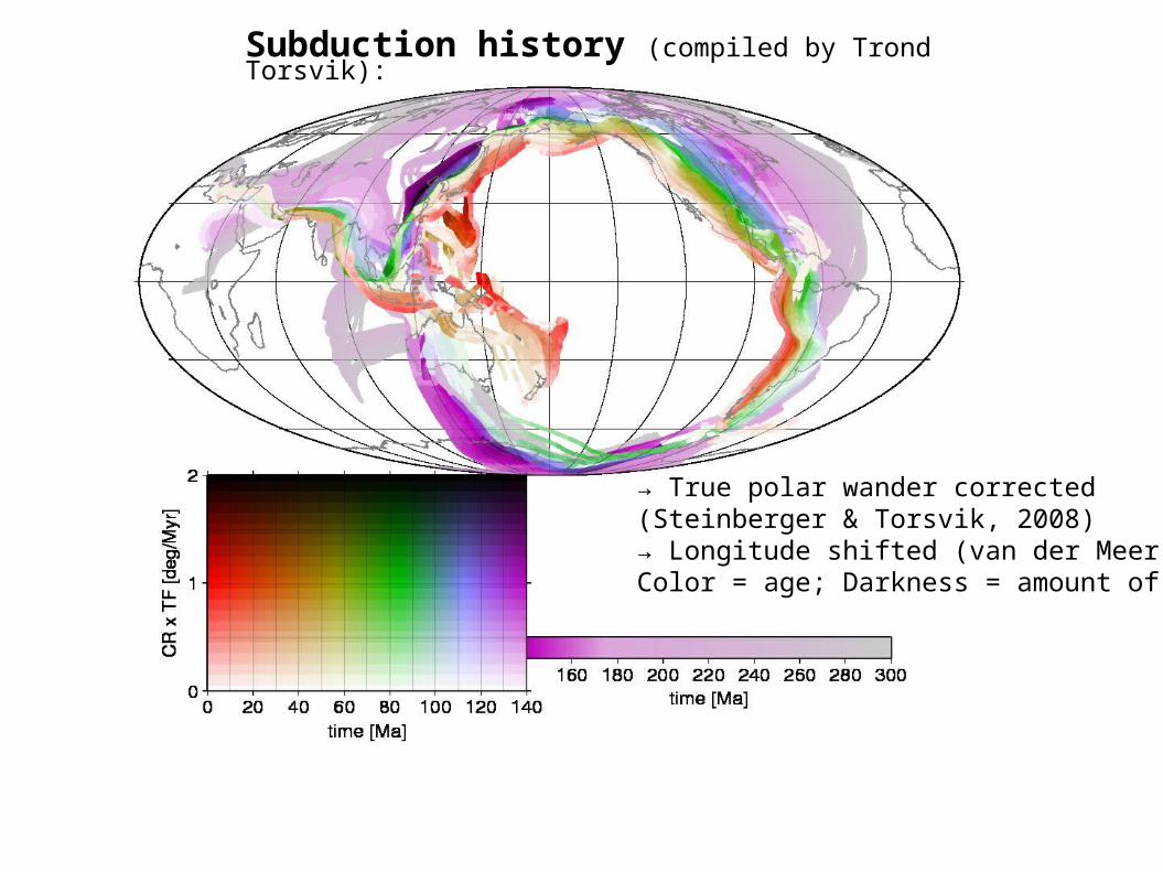
→ True polar wander corrected (Steinberger & Torsvik, 2008)→ Longitude shifted (van der Meer et al., 2010)Color = age; Darkness = amount of subduction

Subduction history (compiled by Trond Torsvik):

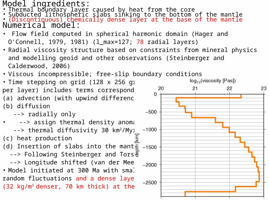
Model ingredients:• Thermal boundary layer caused by heat from the core• Subducted lithospheric slabs sinking to the bottom of the mantle• (Discontinuous) chemically dense layer at the base of the mantleNumerical model:• Flow field computed in spherical harmonic domain (Hager and O'Connell, 1979,

1981) (l_max=127; 78 radial layers)• Radial viscosity structure based on constraints from mineral physics and modelling

geoid and other observations (Steinberger and Calderwood, 2006)• Viscous incompressible; free-slip boundary conditions• Time stepping on grid (128 x 256 grid points per layer) includes terms corresponding to(a) advection (with upwind differencing scheme)(b) diffusion --> radially only• --> assign thermal density anomaly at CMB --> thermal diffusivity 30 km2/Myr(c) heat production(d) Insertion of slabs into the mantle --> Following Steinberger and Torsvik (2010) --> Longitude shifted (van der Meer et al., 2010)• Model initiated at 300 Ma with small random fluctuations and a dense layer (32 kg/m3 denser, 70 km thick) at the base

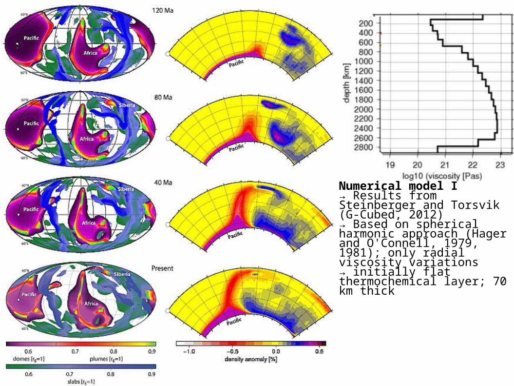
Numerical model I→ Results from Steinberger and Torsvik (G-Cubed, 2012) → Based on spherical harmonic approach (Hager and O'Connell, 1979, 1981); only radial viscosity variations→ initially flat thermochemical layer; 70 km thick

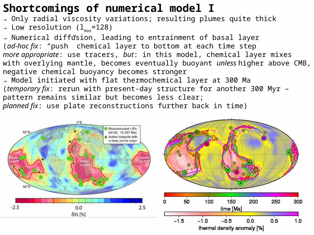
Shortcomings of numerical model I→ Only radial viscosity variations; resulting plumes quite thick → Low resolution (l

max=128)

→ Numerical diffusion, leading to entrainment of basal layer(ad-hoc fix: “push” chemical layer to bottom at each time stepmore appropriate: use tracers, but: in this model, chemical layer mixes with overlying mantle, becomes eventually buoyant unless higher above CMB, negative chemical buoyancy becomes stronger→ Model initiated with flat thermochemical layer at 300 Ma(temporary fix: rerun with present-day structure for another 300 Myr – pattern remains similar but becomes less clear; planned fix: use plate reconstructions further back in time)

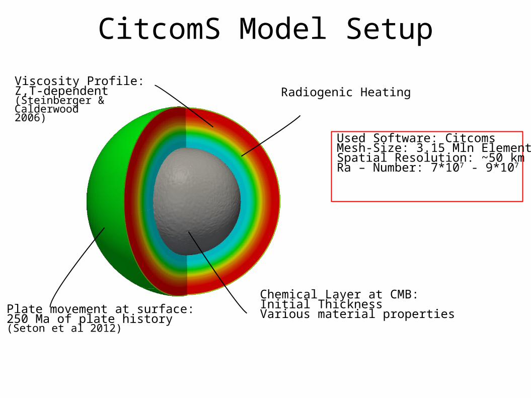
CitcomS Model Setup

Chemical Layer at CMB:Initial ThicknessVarious material properties

Radiogenic Heating

Plate movement at surface:250 Ma of plate history(Seton et al 2012)

Viscosity Profile:Z,T-dependent(Steinberger & Calderwood 2006)

Used Software: CitcomsMesh-Size: 3.15 Mln ElementsSpatial Resolution: ~50 kmRa – Number: 7*107 - 9*107

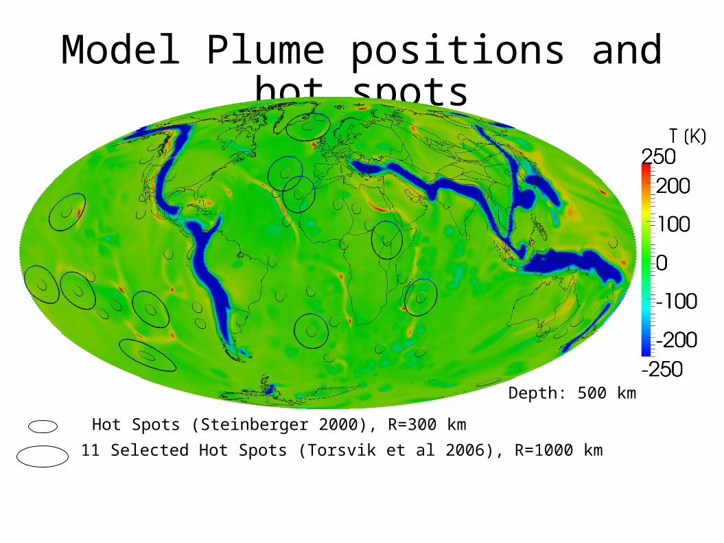
Model Plume positions and hot spots

Hot Spots (Steinberger 2000), R=300 km

11 Selected Hot Spots (Torsvik et al 2006), R=1000 km

Depth: 500 km

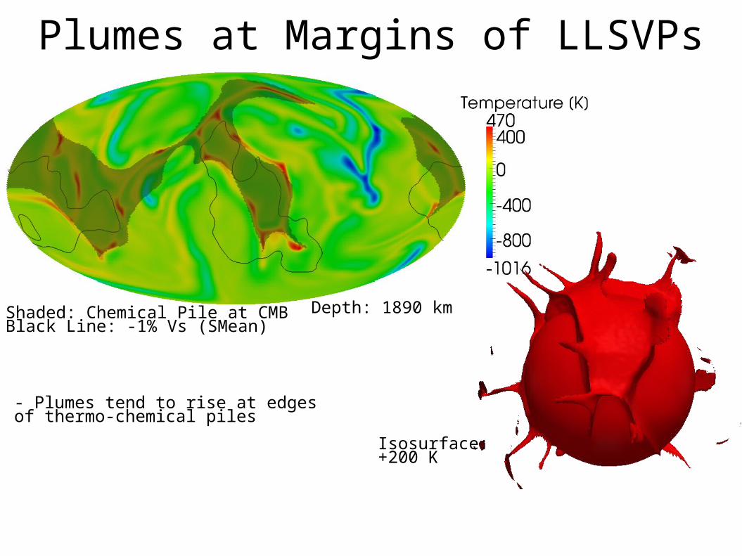
Plumes at Margins of LLSVPs

Depth: 1890 kmShaded: Chemical Pile at CMBBlack Line: -1% Vs (SMean)

Isosurface:+200 K

- Plumes tend to rise at edges of thermo-chemical piles

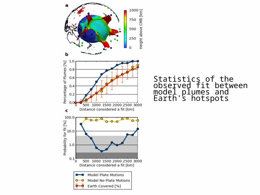
Statistics of the observed fit between model plumes and Earth's hotspots

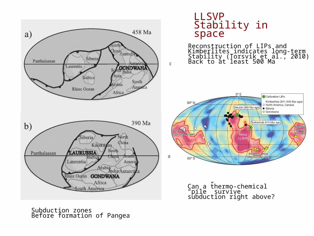
Subduction zonesBefore formation of Pangea

LLSVPStability in space

Reconstruction of LIPs andKimberlites indicates long-termStability (Torsvik et al., 2010) Back to at least 500 Ma

Can a thermo-chemical “pile” survive subduction right above?

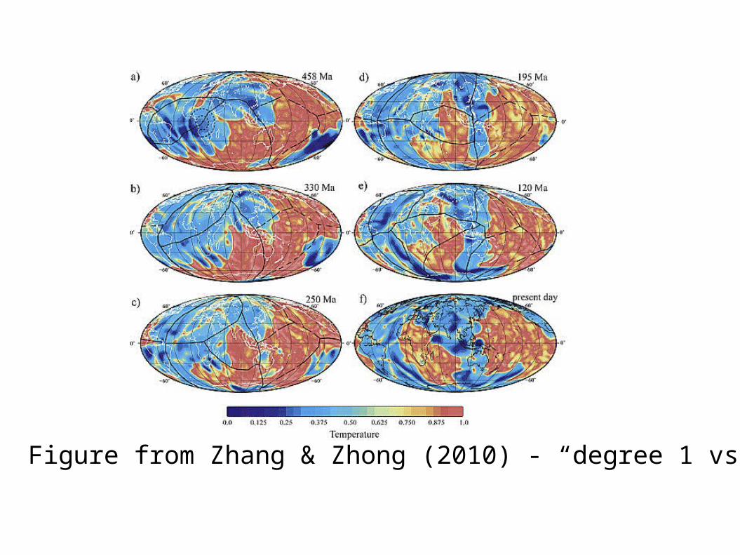
Figure from Zhang & Zhong (2010) - “degree 1 vs. degree 2”

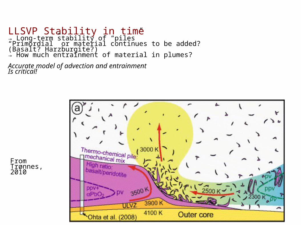
LLSVP Stability in time→ Long-term stability of “piles”“Primordial” or material continues to be added?(Basalt? Harzburgite?)→ How much entrainment of material in plumes?

Accurate model of advection and entrainmentIs critical!

FromTrønnes,2010

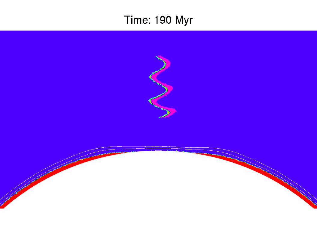
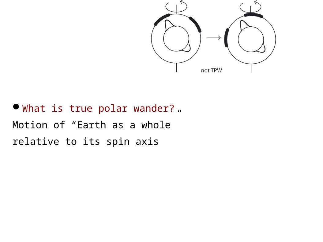
What is true polar wander?

Motion of “Earth as a whole”

relative to its spin axis

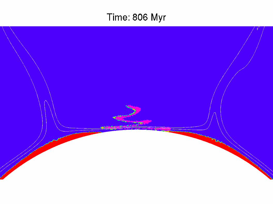
What is true polar wander?

Motion of “Earth as a whole”

relative to its spin axis

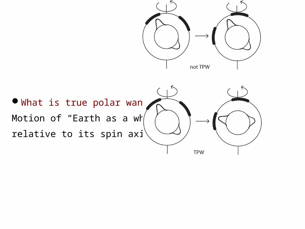
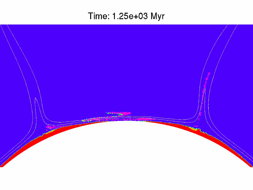
What is true polar wander?

Motion of “Earth as a whole”

relative to its spin axis

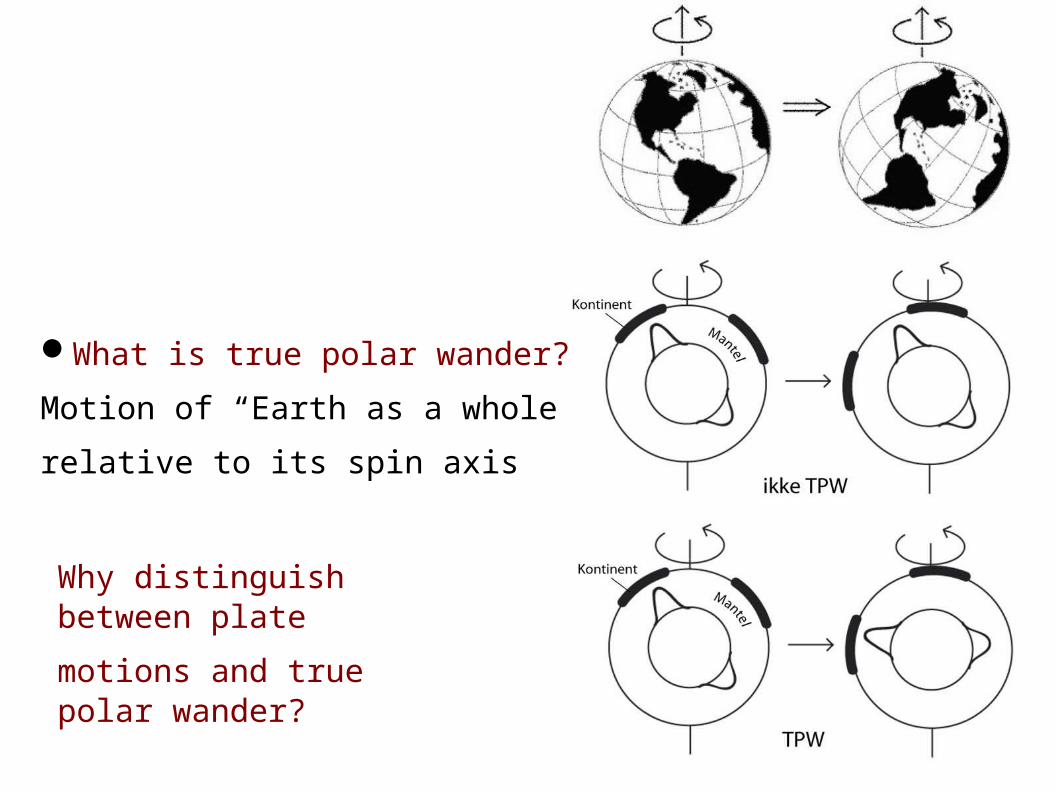
What is true polar wander?

Motion of “Earth as a whole”

relative to its spin axis

Why distinguish between plate

motions and true polar wander?

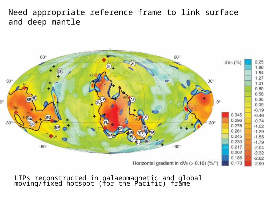
LIPs reconstructed in palaeomagnetic and global moving/fixed hotspot (for the Pacific) frame

Need appropriate reference frame to link surface and deep mantle

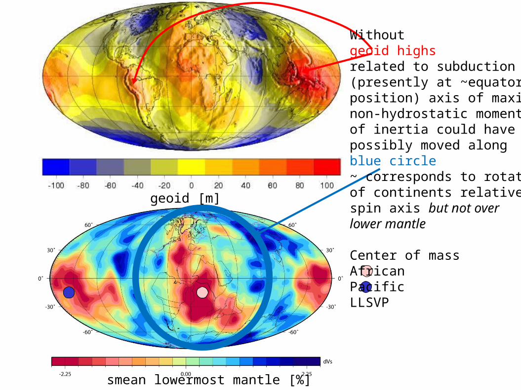
geoid [m]

smean lowermost mantle [%]

Withoutgeoid highsrelated to subduction(presently at ~equatorialposition) axis of maximumnon-hydrostatic momentof inertia could havepossibly moved alongblue circle~ corresponds to rotationof continents relative tospin axis but not overlower mantle

Center of massAfricanPacificLLSVP

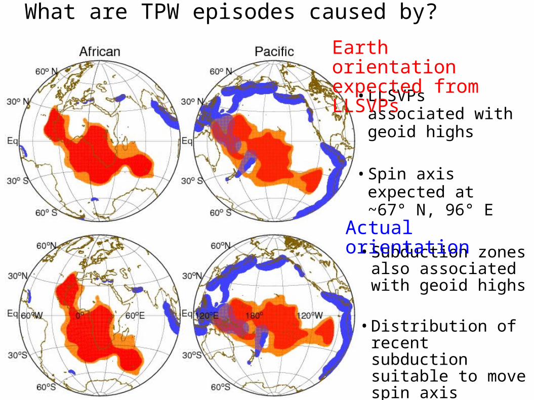
What are TPW episodes caused by?

• LLSVPs associated with geoid highs

• Spin axis expected at ~67° N, 96° E

Earth orientation expected from LLSVPs

• Subduction zones also associated with geoid highs

• Distribution of recent subduction suitable to move spin axis towards observed poles

Actual orientation

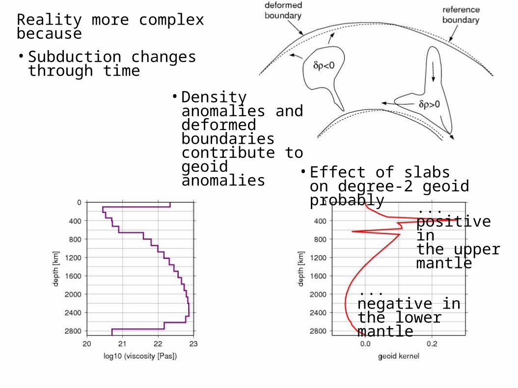
Reality more complex because

• Subduction changes through time

• Density anomalies and deformed boundaries contribute to geoid anomalies

• Effect of slabs on degree-2 geoid probably

... positive in the upper mantle

... negative in the lower mantle

→ True polar wander corrected (Steinberger & Torsvik, 2008)→ Longitude shifted (van der Meer et al., 2010)Color = age; Darkness = amount of subduction

Subduction history (compiled by Trond Torsvik):

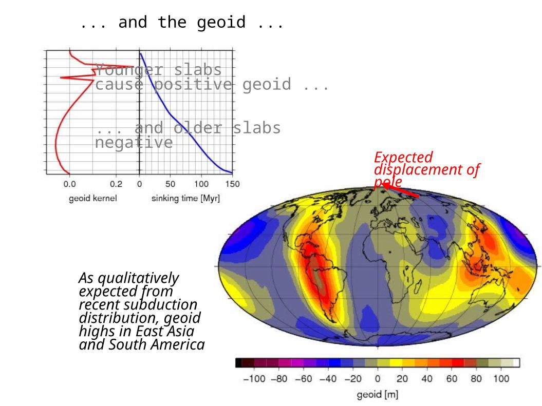
... and the geoid ...

Younger slabscause positive geoid ...

... and older slabsnegative

As qualitatively expected from recent subduction distribution, geoidhighs in East Asiaand South America

Expected displacement of pole

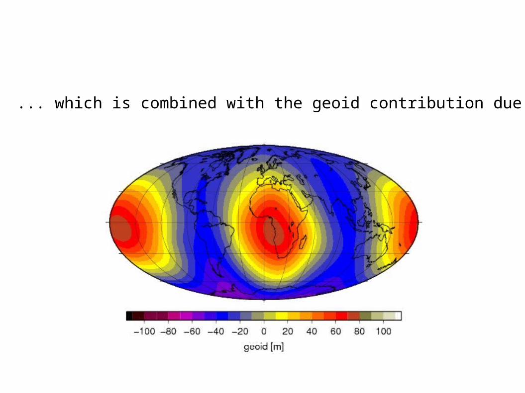
... which is combined with the geoid contribution due to LLSVPs, weighted ...

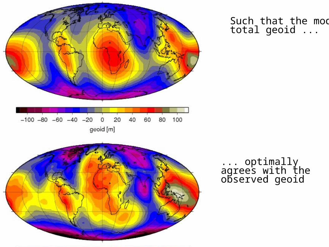
Such that the modelledtotal geoid ...

... optimally agrees with the observed geoid

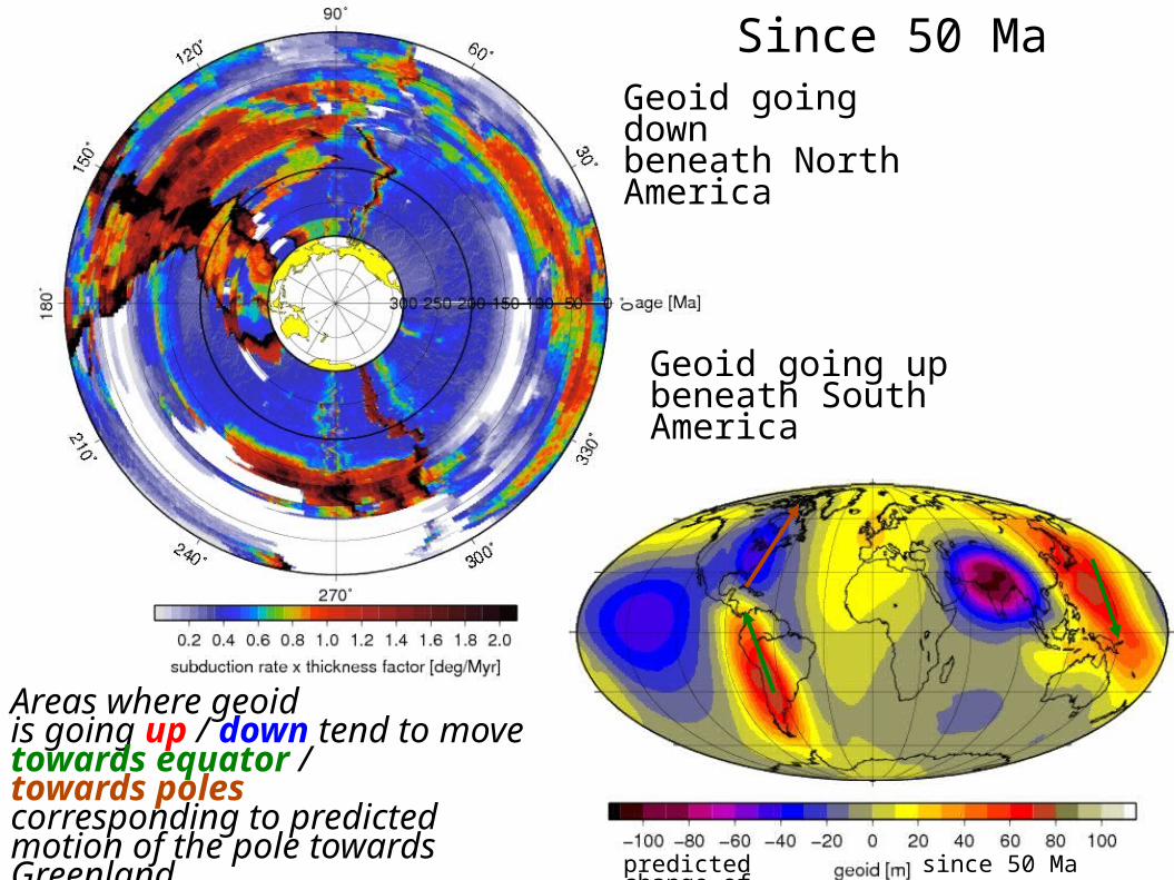
Geoid going up beneath SouthAmerica

Geoid going downbeneath North America

predicted change of since 50 Ma

Areas where geoidis going up / down tend to move towards equator /towards polescorresponding to predicted motion of the pole towards Greenland

Since 50 Ma

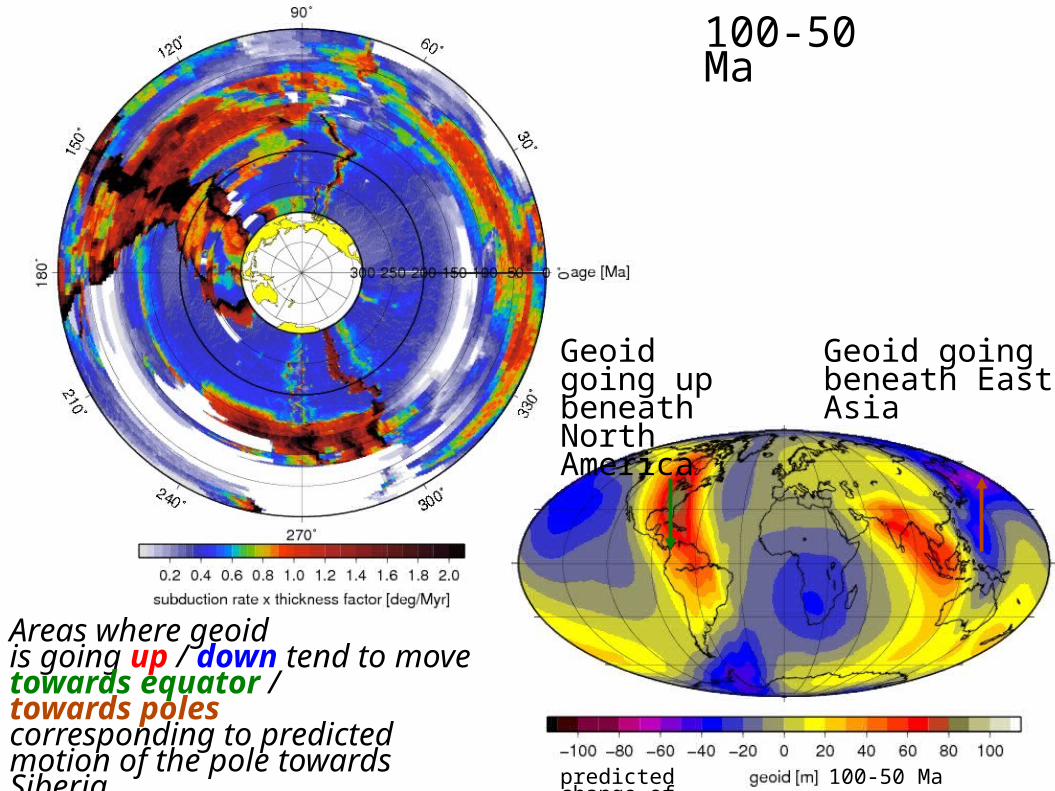
Geoid going downbeneath EastAsia

Geoid going upbeneath North America

predicted change of 100-50 Ma

Areas where geoidis going up / down tend to move towards equator /towards polescorresponding to predicted motion of the pole towards Siberia

100-50 Ma

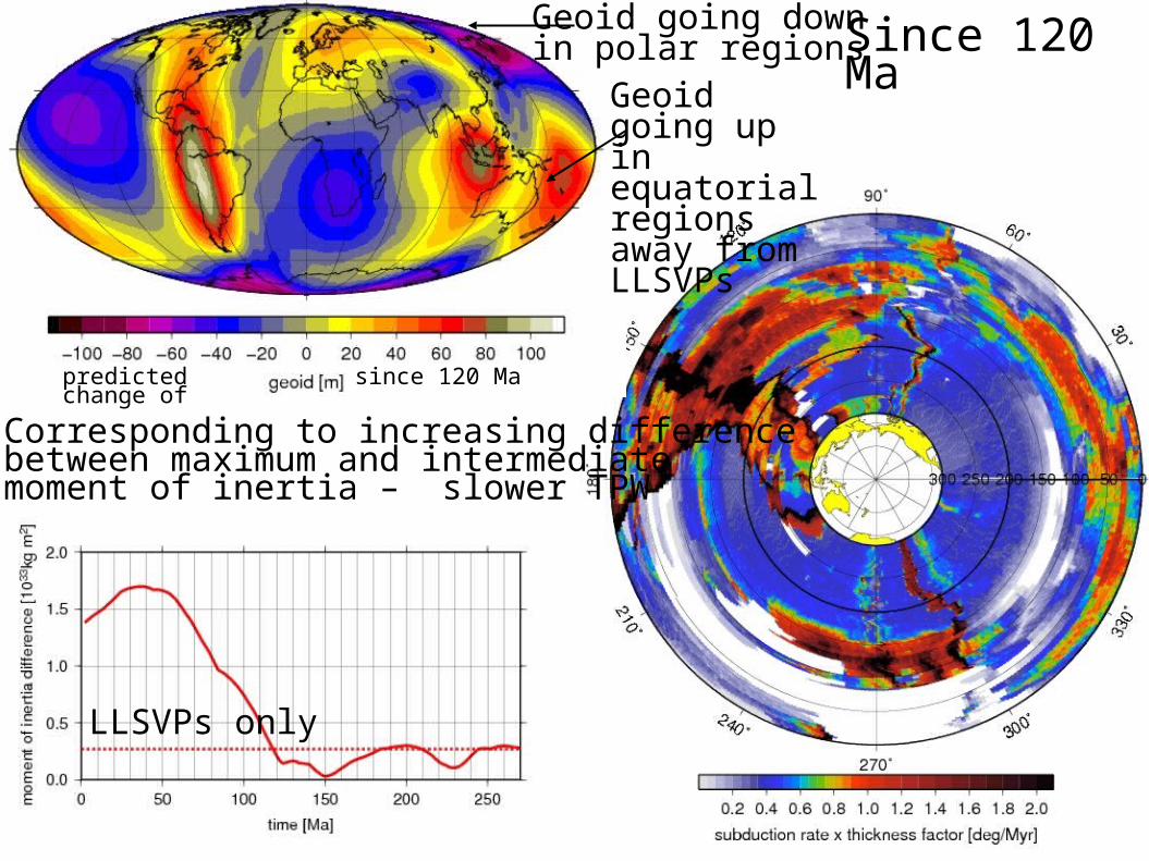
Geoid going downin polar regions

Geoid going upin equatorial regions away from LLSVPs

predicted change of since 120 Ma

Since 120 Ma

Corresponding to increasing differencebetween maximum and intermediatemoment of inertia – slower TPW

LLSVPs only

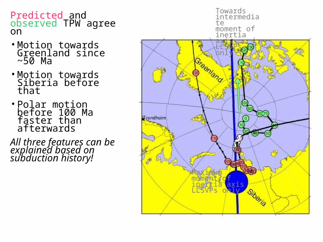
Predicted and observed TPW agree on• Motion towards

Greenland since ~50 Ma• Motion towards Siberia

before that• Polar motion before 100

Ma faster than afterwards

All three features can be explained based on subduction history!

Maximum moment ofinertia axisLLSVPs only

Towards intermediatemoment of inertia axisLLSVPs only

LLSVPs only

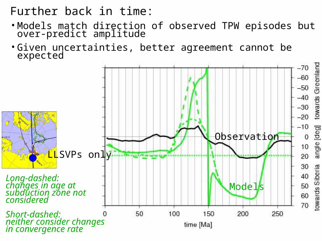
Long-dashed:changes in age at subduction zone not considered

Short-dashed:neither consider changesin convergence rate

Further back in time:• Models match direction of observed TPW episodes but over-predict

amplitude• Given uncertainties, better agreement cannot be expected

Observation

Models

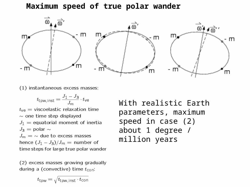
Maximum speed of true polar wander

With realistic Earth parameters, maximum speed in case (2) about 1 degree / million years

Conclusions Plate motions and true polar wander can be distinguished, even in

the absence of hotspot tracks; several episodes of true polar wander are identified (up to 18 degrees, at speeds not exceeding ~1deg/Myr)

Earth’s orientation relative to its spin axis is a consequence of subduction history and stable Large Low Shear Velocity Provinces