Text ClassificationBesat Kassaie

Outline

Introduction

Text classification definition

Naive Bayes

Vector Space Classification

Rocchio Classficiation

KNN Classification

New Applications

2

Spam Detection3

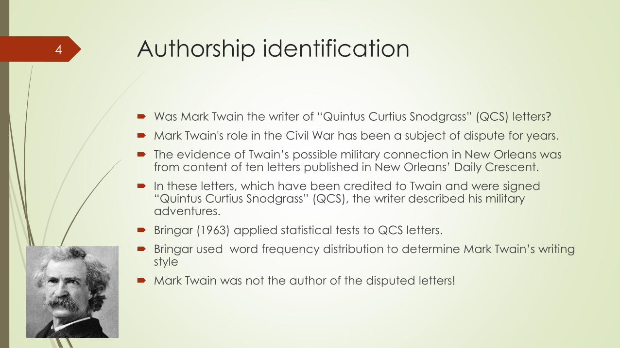
Authorship identification

Was Mark Twain the writer of “Quintus Curtius Snodgrass” (QCS) letters?

Mark Twain's role in the Civil War has been a subject of dispute for years.

The evidence of Twain’s possible military connection in New Orleans was from content of ten letters published in New Orleans’ Daily Crescent.

In these letters, which have been credited to Twain and were signed “Quintus Curtius Snodgrass” (QCS), the writer described his military adventures.

Bringar (1963) applied statistical tests to QCS letters.

Bringar used word frequency distribution to determine Mark Twain’s writing style

Mark Twain was not the author of the disputed letters!

4

Gender Identification

Determining if an author is male or female

Men and women inherently use different classes of language styles.

Samples:

a large number of determiners (a, the, that, these) and quantifiers (one, two,

more, some) are male indicators.

Using large number of the pronouns (I, you, she, her, their, myself, yourself,

herself) are all strong female indicators.

Applications:

Marketing, personalization, legal investigation

5

Sentiment Analysis

Is the attitude of this text positive or negative?

Rank the attitude of this text from 1 to 5

Sample Applications:

Movie: is this review positive or negative?

Products: what do people think about the new iPhone?

Public sentiment: how is consumer confidence? Is despair increasing?

Politics: what do people think about this candidate or issue?

Prediction: predict election outcomes or market trends from sentiment

6

Subject Assignment

What is the subject of this article:

Antagonists and inhibitors

Blood Supply

Chemistry

Drug Therapy

Embryology

….

??

7

Text Classification Definition

Input:

a document d

a fixed set of classes C={c1,c2,…,cj}

Output: a predicted class c ∈ C

8

Approaches to Text Classification

Manual

Many classification tasks have traditionally been solved manually.

e.g. Books in a library are assigned Library of Congress categories by a librarian

manual classification is expensive to scale

Hand-crafted rules

A rule captures a certain combination of keywords that indicates a class.

e.g. (multicore OR multi-core) AND (chip OR processor OR microprocessor)

good scaling properties

creating and maintaining them over time is labor intensive

Machine learning based methods

9

Supervised Learning

Input:

a document d

a fixed set of classes C={c1,c2,…,cj}

a training set of m labeled documents (d1,c1), (d2,c2),…,(dm,cm)

Output: a learned classifier γ :d → c

10

Supervised Learning

We can use any kind of classifiers:

Naïve bayes

kNN

Rocchio

SVM

Logistic Regression

….

11

Naïve Bayes Classification

12

Naïve Bayes Intuition

It is a simple classification technique based on Bayes rule

Documents are represented by “bag of words” model

The bag of words model :

a document d, is represented by the set of words and their weights

determined by the TF weights

TF is the number of occurrences of each term.

The document “Mary is quicker than John” is, in this view, identical to

the document “John is quicker than Mary”.

13

The bag of words representation

I love this movie! It's sweet, but with satirical humor. The dialogue is great and the adventure scenes are fun… It manages to be whimsical and romantic while laughing at the conventions of the fairy tale genre. I would recommend it to just about anyone. I've seen it several times, and I'm always happy to see it again whenever I have a friend who hasn't seen it yet.

γ( )=c

14

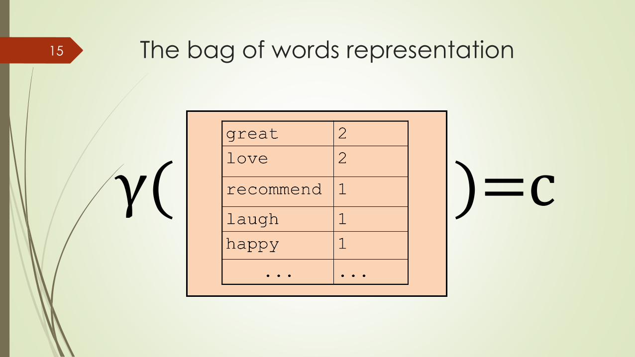
The bag of words representation

γ( )=c

15

Features

Supervised learning classifiers can use any sort of feature

URL, email address, punctuation, capitalization, social network features

and so on

In the bag of words view of documents

We use only word features

16

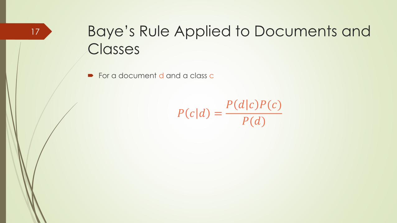
Baye’s Rule Applied to Documents and

Classes

For a document d and a class c

𝑃 𝑐 𝑑 =𝑃 𝑑 𝑐 𝑃(𝑐)

𝑃(𝑑)

17

Naïve Bayes Classifier

𝑐𝑚𝑎𝑝 = 𝑎𝑟𝑔𝑚𝑎𝑥𝑐∈𝐶

𝑝 𝑐 𝑑

= 𝑎𝑟𝑔𝑚𝑎𝑥𝑐∈𝐶

𝑃 𝑑 𝑐 𝑃(𝑐)

𝑃(𝑑)

= 𝑎𝑟𝑔𝑚𝑎𝑥𝑐∈𝐶

𝑃 𝑑 𝑐 𝑃(𝑐)

= 𝑎𝑟𝑔𝑚𝑎𝑥𝑐∈𝐶

𝑃 𝑥1, 𝑥1 , … , 𝑥𝑛 𝑐 𝑃(𝑐)

MAP is “maximum a

posteriori” = most

likely class

Bayes Rule

Dropping the

denominator

Document d

represented as Features

x1..xn

18

Multinomial NB VS Bernoulli NB

There are two different approaches for setting up an NB classifier.

multinomial model: generates one term from the vocabulary in each

position of the document

multivariate Bernoulli model: generates an indicator for each term of the vocabulary, either 1 indicating presence of the term in the document or 0

indicating absence

Difference in estimation strategies

19

Document Features

𝑐𝑚𝑎𝑝=𝑎𝑟𝑔𝑚𝑎𝑥𝑐∈𝐶

𝑃 𝑑 𝑐 𝑃(𝑐)

Multinomial:

𝑐𝑚𝑎𝑝 = 𝑎𝑟𝑔𝑚𝑎𝑥𝑐∈𝐶

𝑃 𝑤1, 𝑤2 , … , 𝑤𝑛 𝑐 𝑃(𝑐)

𝑤1, 𝑤2 , … , 𝑤𝑛 is the sequence of terms as it occurs in d

Bernoulli:

𝑐𝑚𝑎𝑝 = 𝑎𝑟𝑔𝑚𝑎𝑥𝑐∈𝐶

𝑃 𝑒1, 𝑒2 , … , 𝑒𝑣 𝑐 𝑃(𝑐)

𝑒1, 𝑒2 , … , 𝑒𝑣 is a binary vector of dimensionality V that indicates for each

term whether it occurs in d or not

20

ASSUMPTIONS: Conditional independence

𝑃 𝑥1, 𝑥2 , … , 𝑥𝑛 𝑐 = 𝑃 𝑥1 𝑐 ∙ 𝑃 𝑥2 𝑐 ∙ ⋯ ∙ 𝑃 𝑥𝑛 𝑐

Multinomial:

𝑐𝑚𝑎𝑝 = 𝑎𝑟𝑔𝑚𝑎𝑥𝑐∈𝐶

𝑃 𝑤1, 𝑤2 , … , 𝑤𝑛 𝑐 𝑃 𝑐

𝑐𝑁𝐵 = 𝑎𝑟𝑔𝑚𝑎𝑥𝑐∈𝐶

1≤𝑘≤𝑛 𝑃 𝑋𝑘 = 𝑤𝑘 𝑐 𝑃(𝑐)

Xk is the random variable for position k in the document and takes

as values terms from the vocabulary.

𝑃 𝑋𝑘 = 𝑤𝑘 𝑐 is the probability that in a document of class c the term

w will occur in position k

21

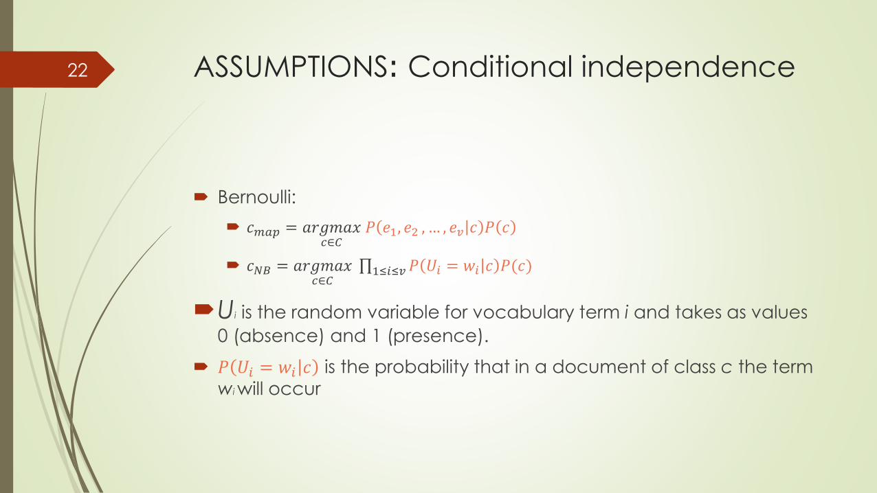
ASSUMPTIONS: Conditional independence

Bernoulli:

𝑐𝑚𝑎𝑝 = 𝑎𝑟𝑔𝑚𝑎𝑥𝑐∈𝐶

𝑃 𝑒1, 𝑒2 , … , 𝑒𝑣 𝑐 𝑃 𝑐

𝑐𝑁𝐵 = 𝑎𝑟𝑔𝑚𝑎𝑥𝑐∈𝐶

1≤𝑖≤𝑣 𝑃 𝑈𝑖 = 𝑤𝑖 𝑐 𝑃(𝑐)

Ui is the random variable for vocabulary term i and takes as values

0 (absence) and 1 (presence).

𝑃 𝑈𝑖 = 𝑤𝑖 𝑐 is the probability that in a document of class c the term

wi will occur

22

ASSUMPTIONS: Bag of words

assumption

if we assumed different term distributions for each position k, we would have to estimate a different set of parameters for each k

positional independence: The conditional probabilities for a term are the same, independent of position in the document.

E.g. P(Xk1 = t|c) = P(Xk2 = t|c)

we have a single distribution of terms that is valid for all positions k

𝑐𝑚𝑎𝑝 = 𝑎𝑟𝑔𝑚𝑎𝑥𝑐∈𝐶

𝑃 𝑤1, 𝑤2 , … , 𝑤𝑛 𝑐 𝑃 𝑐

𝑐𝑁𝐵 = 𝑎𝑟𝑔𝑚𝑎𝑥𝑐∈𝐶

𝑤𝜖𝑊

𝑃 𝑤 𝑐 𝑃(𝑐)

23

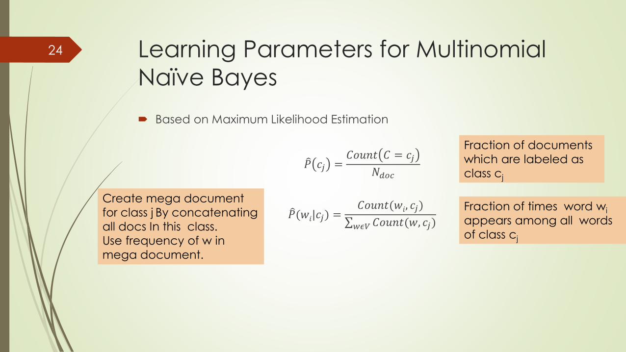
Learning Parameters for Multinomial

Naïve Bayes

Based on Maximum Likelihood Estimation

𝑃 𝑐𝑗 =𝐶𝑜𝑢𝑛𝑡 𝐶 = 𝑐𝑗

𝑁𝑑𝑜𝑐

𝑃(𝑤𝑖|𝑐𝑗) =𝐶𝑜𝑢𝑛𝑡(𝑤𝑖, 𝑐𝑗)

𝑤𝜖𝑉 𝐶𝑜𝑢𝑛𝑡(𝑤, 𝑐𝑗)

Fraction of times word wi

appears among all words

of class cj

Create mega document

for class j By concatenating

all docs In this class.

Use frequency of w in

mega document.

24

Fraction of documents

which are labeled as

class cj

Laplace (add-1) smoothing for Naïve

Bayes

Solving the problem of zero probabilities

𝑃 𝑤𝑖 𝑐𝑗 =𝐶𝑜𝑢𝑛𝑡 𝑤𝑖, 𝑐𝑗 + 1

𝑤𝜖𝑉 𝐶𝑜𝑢𝑛𝑡 𝑤, 𝑐𝑗 + 1

=𝐶𝑜𝑢𝑛𝑡 𝑤𝑖, 𝑐𝑗 + 1

𝑤𝜖𝑉 𝐶𝑜𝑢𝑛𝑡 𝑤, 𝑐𝑗 + |𝑉|

25

Laplace (add-1) smoothing: unknown

words

Add one extra word to the vocabulary, the “unknown word” , wu

𝑃 𝑤𝑢 𝑐𝑗 =𝐶𝑜𝑢𝑛𝑡 𝑤𝑢, 𝑐𝑗 + 1

( 𝑤𝜖𝑉 𝑐𝑜𝑢𝑛𝑡(𝑤, 𝑐𝑗)) + |𝑉 + 1|

=1

( 𝑤𝜖𝑉 𝑐𝑜𝑢𝑛𝑡(𝑤, 𝑐𝑗)) + |𝑉 + 1|

Probability for all unknown words

26

Example27

Vector Space Classification

28

Vector Space Representation

The document representation in Naive Bayes is a sequence of terms or a binary vector

A different representation for text classification: the vector space model

Each document represented as a vector with one real-valued component,

usually a tf-idf weight, for each term.

Each vector is composed of all terms

Of all documents.

Terms are axis

High dimensionality

29

Vector Space Classification

Vector space classification is based on the contiguity hypothesis:

Objects in the same class form a contiguous region, and regions of different

classes do not overlap

Classification is to compute the boundaries in the space that separate the

classes; the decision boundaries

Two methods will be discussed:

Rocchio and kNN

30

Vector Space Classification

Rocchio

31

Rocchio Classification

Basic idea: Rocchio forms a simple representative for each class by using

the centroids.

To compute the centroid of each class:

𝜇 𝑐 =1

|𝐷𝑐| 𝑑𝜖𝐷𝑐 𝑣(𝑑)

Dc is the set of all documents that belong to class c

v(d) is the vector space representation of d.

32

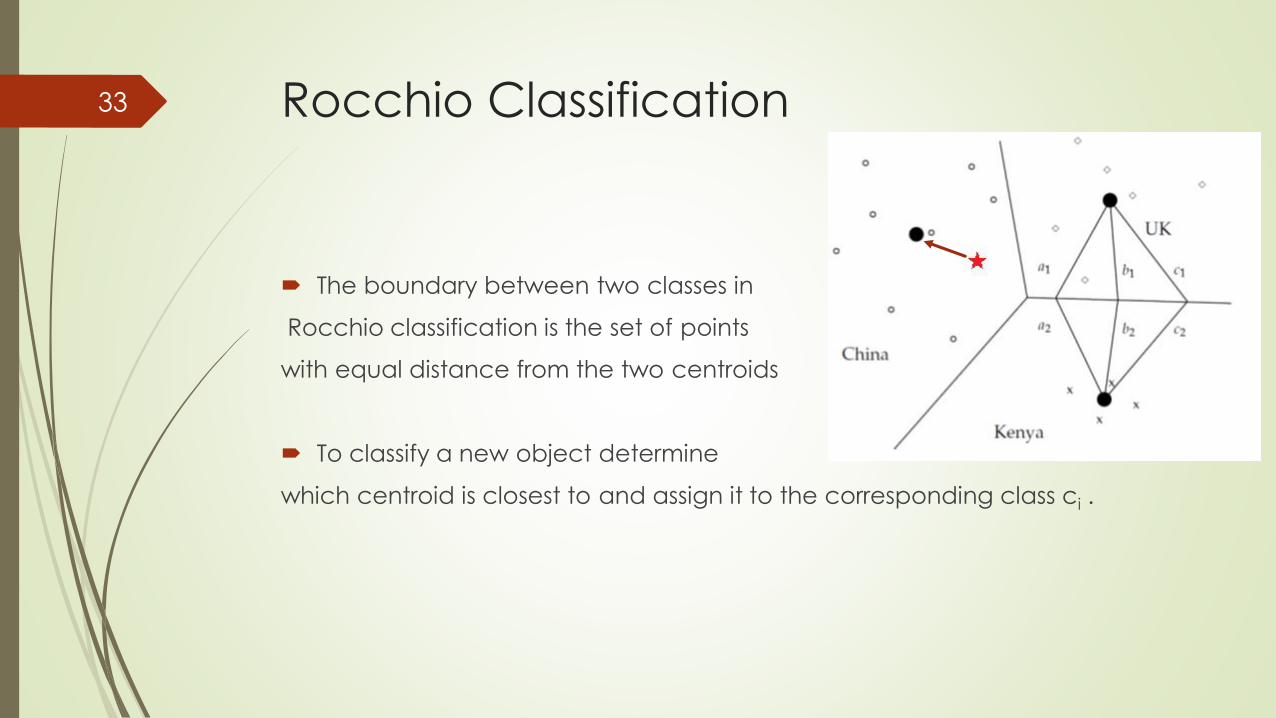
Rocchio Classification

The boundary between two classes in

Rocchio classification is the set of points

with equal distance from the two centroids

To classify a new object determine

which centroid is closest to and assign it to the corresponding class ci .

33

Problems with Rocchio Classification

Implicitly assumes that classes are spheres with similar radius

Ignores details of distribution of points within a class and only considers

centroid distances.

Red cube is assigned to Kenya class

But is a better fit for UK class

since UK is more scattered than Kenya

Not requiring similar radius → modified decision rule:

Assign d to class c iff 𝜇 𝑐 − 𝑣 𝑑 ≤ 𝜇 𝑐 − 𝑣 𝑑 − 𝑏

34

Problems with Rocchio Classification

Does not work well for classes than cannot be accurately represented by a

single “center”

Class “a” consists of two different clusters.

Rocchio classification will misclassify “o” as “a” because

it is closer to the centroid A of the “a” class than to the

centroid B of the “b” class.

35

Vector Space Classification

K Nearest Neighbor

36

K Nearest Neighbor Classification

For kNN we assign each document to the majority class of its k closest

neighbors where k is a parameter.

The rationale of kNN classification is that, based on the contiguity

hypothesis, we expect a test document d to have the same label as the

training documents located in the local region surrounding d.

Learning: just store the labeled training examples D

37

K Nearest Neighbor Classification

Determining class of a new document :

For k = 1: Assign each object to the class of its closest neighbor.

For k > 1: Assign each object to the majority class among its k closest

neighbors.

The parameter k must be specified in advance. k = 3 and k = 5 are

common choices, but much larger values between 50 and 100 are also

used

38

kNN decision boundary

The decision boundary defined by the Voronoi tessellation

Assuming k = 1: For a given set of objects in the space, each object define a cell consisting of all points that are closer to that object than to other objects.

Results in a set of convex polygons;

so-called Voronoi cells.

Decomposing a space into such cells

gives us the so-called Voronoi tessellation.

In the case of k > 1, the Voronoi cells

are given by the regions in the space for which

the set of k nearest neighbors is the same.

39

Decision boundary for 1NN (double line): defined along the regions of

Voronoi cells for the objects in each class. Shows the non-linearity of kNN

40

kNN: Probabilistic version

There is a probabilistic version of kNN classification algorithm.

We can estimate the probability of membership in class c as the proportion of the k nearest neighbors in c.

𝑃 (𝑐𝑖𝑟𝑐𝑙𝑒 𝑐𝑙𝑎𝑠𝑠|𝑠𝑡𝑎𝑟) = 1/3

𝑃(𝑋 𝑐𝑙𝑎𝑠𝑠|𝑠𝑡𝑎𝑟) = 2/3

𝑃(𝑑𝑖𝑎𝑚𝑜𝑛𝑑 𝑐𝑙𝑎𝑠𝑠|𝑠𝑡𝑎𝑟) = 0

The 3NN estimate: 𝑃(𝑐𝑖𝑟𝑐𝑙𝑒 𝑐𝑙𝑎𝑠𝑠|𝑠𝑡𝑎𝑟) = 1/3

The 1NN estimate: 𝑃(𝑐𝑖𝑟𝑐𝑙𝑒 𝑐𝑙𝑎𝑠𝑠|𝑠𝑡𝑎𝑟) = 1

3NN preferring the X class

and 1NN preferring the circle class .

41

kNN: distance weighted version

We can weight the “votes” of the k nearest neighbors by their cosine

similarity:

𝑆𝑐𝑜𝑟𝑒(𝑐, 𝑑) = 𝑑𝜖𝑆𝑘(𝑑)

𝐼𝑐 𝑑 cos( 𝑣 𝑑 , 𝑣 𝑑 )

Sk(d) is the set of d’s k nearest neighbors

Ic(d′) = 1 iff d′ is in class c and 0 otherwise.

Assign the document to the class with the highest score.

Weighting by similarities is often more accurate than simple voting.

42

kNN Properties

No training necessary

Scales well with large number of classes

Don’t need to train n classifiers for n classes

May be expensive at test time

In most cases it’s more accurate than NB or Rocchio

43

Some Recent Applications of Text

Classification

Social networks are rich source of text data e.g. twitter

Many new applications are emerging based on these sources

We will discuss three recent works based on twitter data

“Learning Similarity Functions for Topic Detection in Online Reputation

Monitoring. Damino Spina, et. Al, SIGIR, 2014”

“Target-dependent Churn Classification in Microblogs, Hadi Amiri, et.al,

AAAI 2015”

“Fine-Grained Location Extraction from Tweets with Temporal Awareness,

Chenliang Li, SIGIR, 2014”

44

Learning Similarity Functions for Topic

Detection in Online Reputation Monitoring

What are people are saying about a given entity (company, brand,

organization, personality,…)

Is there any issues that may damage the reputation of the entity?

In order to answer such questions, reputation experts have to daily monitor

social networks such as twitter

The paper aim is to solve this problem automatically as topic detection task

Reputation alerts must be detected early before they explode. So there are

a few number of related tweets

Probabilistic generative approaches are less appropriate here because of

data sparsity

45

Learning Similarity Functions…

Paper proposes a hybrid approach: supervised + unsupervised

Tweets need to be clustered based on their topics

Clusters change over time based on data stream

Tweets with similar topics belong to the same cluster

For clustering we need a similarity function.

Classification (SVM) is used to learn the similarity function.

Two tweets belong to either similar or not similar classes

SVM

Hierarchical Agglomerative Clustering

46

Learning Similarity Functions…

Dataset is comprised of 142,527 manually annotated tweets.

Features used for classification:

Term Features:

taking into account similarity between terms in the tweets

Tweets sharing high percentage of vocabulary are likely about same topic

Semantic features:

Useful for tweets that do not have words in common.

Used Wikipedia as a knowledge based to find semantically related words. e.g. mexico, mexicanas

Metadata features:

Such as author, URLs, hashtags,…

Time-aware features:

Time stamp of tweets

47

Fine-Grained Location Extraction from

Tweets with Temporal Awareness

Through tweets, users often casually or implicitly reveal their current

locations and short term plans where to visit next, at fine-grained granularity

Such information enables tremendous opportunities for personalization and

location-based services/marketing

This paper is about extracting fine-grained locations mentioned in tweets

with temporal awareness.

48

Fine-Grained Location Extraction…

Dataset: a sample of 4000 manually annotated tweets

Classifier: Conditional Random Fields

Some features:

Lexical Features: words itself, its lower case, bag-of-words of the context window,

Grammatical Features: POS tags (for verb tense), word groups (shudd, shuld,

shoud)

…

If a user mentions a point-of-interest (POI) (e.g., restaurant, shopping

mall,…) in her tweet:

The name of the POI is extracted

The tweet is assigned into one of these classes: The POI is visited, is currently at, or

will soon visit (temporal awareness).

49

Target-dependent Churn Classification

in Microblogs

The problem of classifying micro-posts as churny or non-churny with respect

to a given brand (telecom companies) using Twitter data.

Whether a tweet is an indicator that user is going to cancel a service

Sample tweets:

“One of my main goals for 2013 is to leave BrandName”

“I cant take it anymore, the unlimited data isn’t even worth it”

“My days with BrandName are numbered”

50

Target-dependent Churn Classification

in Microblogs

Dataset : 4800 tweets about three telecommunication brands

Classification method: linear regression, SVM, logistic regression

Features:

Demographic Churn Indicators:

Activity ratio (if a user is not active with respect to any competitors, then he is less likely to send churny contents about a target brand),

# followers and friends, …

Content Churn Indicators:

Sentiment features, Tense of tweet,…

…

51

THANK YOU

52

References53

https://web.stanford.edu/class/cs124/lec/sentiment.pptx

https://web.stanford.edu/class/cs124/lec/naivebayes.pdf

An introduction to Information Retrieval, Christopher D. Manning

,Prabhakar Raghavan,Hinrich Schütze,2009

Learning Similarity Functions for Topic Detection in Online

Reputation Monitoring. Damino Spina, et. Al, SIGIR, 2014

Target-dependent Churn Classification in Microblogs, Hadi Amiri,

et.al, AAAI 2015

Fine-Grained Location Extraction from Tweets with Temporal

Awareness, Chenliang Li, SIGIR, 2014