Best Experienced Payoff Dynamics andCooperation in the Centipede Game∗

William H. Sandholm†, Segismundo S. Izquierdo‡, and Luis R. Izquierdo§

February 8, 2018

Abstract

We study population game dynamics under which each revising agent randomlyselects a set of strategies according to a given test-set rule, plays each strategy inthis set a fixed number of times, with each play of each strategy being against anewly drawn opponent, and chooses the strategy whose total payoff was highest,breaking ties according to a given tie-breaking rule. In the Centipede game, thesebest experienced payoff dynamics lead to cooperative play. Play at the almost globallystable state is concentrated on the last few nodes of the game, with the proportionsof agents playing each strategy being dependent on the specification of the dynamics,but largely independent of the length of the game. The emergence of cooperativeplay is robust to allowing agents to test candidate strategies many times, and tointroducing substantial proportions of agents who always stop immediately. Since bestexperienced payoff dynamics are defined by random sampling procedures, they arerepresented by systems of polynomial differential equations with rational coefficients,allowing us to establish key properties of the dynamics using tools from computationalalgebra.

∗We thank Ken Judd, Panayotis Mertikopoulos, Erik Mohlin, Ignacio Monzon, Marzena Rostek, ArielRubinstein, Larry Samuelson, Ryoji Sawa, Lones Smith, Mark Voorneveld, Marek Weretka, and especiallyAntonio Penta for helpful discussions and comments. Financial support from the U.S. National ScienceFoundation (SES-1458992 and SES-1728853), the U.S. Army Research Office (MSN201957), project ECO2017-83147-C2-2-P (MINECO/AEI/FEDER, UE), and the Spanish Ministerio de Educacion, Cultura, y Deporte(PRX15/00362 and PRX16/00048) is gratefully acknowledged.†Department of Economics, University of Wisconsin, 1180 Observatory Drive, Madison, WI 53706, USA.

e-mail: whs@ssc.wisc.edu; website: www.ssc.wisc.edu/˜whs.‡Department of Industrial Organization, Universidad de Valladolid, Paseo del Cauce 59, 47011 Val-

ladolid, Spain. e-mail: segis@eis.uva.es; website: www.segis.izqui.org.§Department of Civil Engineering, Universidad de Burgos, Edificio la Milanera, Calle de Villadiego,

09001 Burgos, Spain. e-mail: lrizquierdo@ubu.es; website: www.luis.izqui.org.

1. Introduction

The discrepancy between the conclusions of backward induction reasoning and ob-served behavior in certain canonical extensive form games is a basic puzzle of game theory.The Centipede game (Rosenthal (1981)), the finitely repeated Prisoner’s Dilemma, and re-lated examples can be viewed as models of relationships in which each participant hasrepeated opportunities to take costly actions that benefit his partner, and in which thereis a commonly known date at which the interaction will end. Experimental and anecdo-tal evidence suggests that cooperative behavior may persist until close to the exogenousterminal date (McKelvey and Palfrey (1992)). But the logic of backward induction leadsto the conclusion that there will be no cooperation at all.

Work on epistemic foundations provides room for wariness about unflinching appealsto backward induction. To support this prediction, one must assume that there is alwayscommon belief that all players will act as payoff maximizers at all points in the future, evenwhen many rounds of previous choices argue against such beliefs.1 Thus the simplicityof backward induction belies the strength of the assumptions needed to justify it, and thisstrength may help explain why backward induction does not yield descriptively accuratepredictions in some classes of games.2

This paper studies a dynamic model of behavior in games that maintains the as-sumption that agents respond optimally to the information they possess. But rather thanimposing strong assumptions about agents’ knowledge of opponents’ intentions, we sup-pose instead that agents’ information comes from direct but incomplete experience withplaying the strategies available to them. As with earlier work of Osborne and Rubinstein(1998) and Sethi (2000), our model is best viewed not as one that incorporates irrationalchoices, but rather as one of rational choice under particular restrictions on what agentsknow.

Following the standard approach of evolutionary game theory, we suppose that twopopulations of agents are recurrently randomly matched to play a two-player game.This framework accords with some experimental protocols, and can be understood morebroadly as a model of the formation of social norms (Young (1998)). At random times,each agent receives opportunities to switch strategies. At these moments the agent decideswhether to continue to play his current strategy or to switch to an alternative in a testset, which is determined using a prespecified stochastic rule τ. The agent then plays

1For formal analyses, see Binmore (1987), Reny (1992), Stalnaker (1996), Ben-Porath (1997), Halpern(2001), and Perea (2014).

2As an alternative, one could apply Nash equilibrium, which also predicts noncooperative behavior inthe games mentioned above, but doing so replaces assumptions about future rationality with the assumptionof equilibrium knowledge, which may not be particularly more appealing—see Dekel and Gul (1997).

–2–

each strategy he is considering against κ opponents drawn at random from the opposingpopulation, with each play of each strategy being against a newly drawn opponent. Hethen switches to the strategy that achieved the highest total payoff, breaking ties accordingto a prespecified rule β.3

Standard results imply that when the populations are large, the agents’ aggregatebehavior evolves in an essentially deterministic fashion, obeying a differential equationthat describes the expected motion of the stochastic process described above (Benaım andWeibull (2003)). The differential equations generated by the protocol above, and our objectof study here, we call best experienced payoff dynamics, or BEP dynamics for short.

Our model builds on earlier work on games played by “procedurally rational players”.In particular, when the test-set rule τ specifies that agents always test all strategies, andwhen the tie-breaking rule β is uniform randomization, then the rest points of our process(with κ = k) are the S(k) equilibria of Osborne and Rubinstein (1998). The correspondingdynamics were studied by Sethi (2000). The analyses in these papers differ substantiallyfrom ours, as we explain carefully below.

Our analysis of best experienced payoff dynamics in the Centipede game uses tech-niques from dynamical systems theory. What is more novel is our reliance on algorithmsfrom computational algebra and perturbation bounds from linear algebra, which allowus to solve exactly for the rest points of our differential equations and to perform rigorousstability analyses. We complement this approach with numerical analyses of cases inwhich analytical results cannot be obtained.

Most of our results focus on dynamics under which each tested strategy is tested ex-actly once (κ = 1), so that agents’ choices only depend on ordinal properties of payoffs.In Centipede games, under BEP dynamics with tie-breaking rules that do not abandonoptimal strategies, or that break ties in favor of less cooperative strategies, the back-ward induction state—the state at which all agents in both populations stop at their firstopportunity—is a rest point. However, we prove that this rest point is always repelling: theappearance of agents in either population who cooperate to any degree is self-reinforcing,and eventually causes the backward induction solution to break down completely.

For all choices of test-set and tie-breaking rules we consider, the dynamics have exactlyone other rest point.4 Except in games with few decision nodes, the form of this rest pointis essentially independent of the length of the game. In all cases, the rest point has virtually

3Tie-breaking rules are important in the context of extensive form games, where different strategies thatagree on the path of play earn the same payoffs.

4While traditional equilibrium notions in economics require stasis of choice, interior rest points ofpopulation dynamics represent situations in which individuals’ choices fluctuate even as the expectedchange in aggregate behavior is null—see Section 2.3.

–3–

all players choosing to continue until the last few nodes of the game, with the proportionsplaying each strategy depending on the test-set and tie-breaking rules. Moreover, this restpoint is dynamically stable, attracting solutions from all initial conditions other than thebackward induction state. Thus under a range of specifications, if agents make choicesbased on experienced payoffs, testing each strategy in their test sets once and choosingthe one that performed best, then play converges to a stable rest point that exhibits highlevels of cooperation.

To explain why, we first observe that cooperative strategies are most disadvantagedwhen they are most rare—specifically, in the vicinity of the backward induction state. Nearthis state, the most cooperative agents would obtain higher expected payoffs by stoppingearlier. However, when an agent considers switching strategies, he tests each strategy inhis test set against new, independently drawn opponents. He may thus test a cooperativestrategy against a cooperative opponent, and less cooperative strategies against less coop-erative opponents, in which case his best experienced payoff will come from the cooperativestrategy. Our analysis confirms that this possibility indeed leads to instability (Sections5 and 6).5 After this initial entry, the high payoffs generated by cooperative strategieswhen matched against one another spurs their continued growth. This growth is onlyabated when virtually all agents are choosing among the most cooperative strategies. Theexact nature of the final mixture depends on the specification of the dynamics, and can beunderstood by focusing on the effects of a small fraction of possible test results (Section5.1.3).

To evaluate the robustness of these results, we alter our model by replacing a fractionof each population with “backward induction agents”. Such agents never consider anybehavior other than stopping at their initial decision node. Despite interactions withinvariably uncooperative agents, the remaining agents persist in behaving cooperatively,with the exact degree depending on the specification of the dynamics and the length ofthe game. For longer games (specifically, games with d = 20 decision nodes), which offermore opportunities for successfully testing cooperative strategies, cooperative behavioris markedly robust, persisting even when two-thirds of the population always stopsimmediately (Section 7).

Our final results consider the effects of the number of trials κ of each strategy in the testset on predictions of play. It seems clear that if the number of trials is made sufficiently

5Specifically, linearizing any given specification of the dynamics at the backward induction state identifiesa single eigenvector with a positive eigenvalue (Appendix A). This eigenvector describes the mixture ofstrategies in the two populations whose entry is self-reinforcing, and identifies the direction toward whichall other disturbances of the backward induction state are drawn. Direct examination of the dynamicsprovides a straightforward explanation why the given mixture of entrants is successful (Example 5.3).

–4–

large, so that the agents’ information about opponents’ behavior is quite accurate, thenthe population’s behavior should come to resemble a Nash equilibrium. Indeed, whenagents possess exact information, so that aggregate behavior evolves according to thebest response dynamic (Gilboa and Matsui (1991), Hofbauer (1995b)), results of Xu (2016)imply that every solution trajectory converges to the set of Nash equilibria, all of whichentail stopping at the initial node.

Our analysis shows, however, that stable cooperative behavior can persist even forsubstantial numbers of trials. In the Centipede games of length d = 4 that we consider inthis analysis, a unique, attracting interior rest point with substantial cooperation persistsfor moderate numbers of trials. For larger numbers of trials, the attractor is always a cycle,and includes significant amounts of cooperation for numbers of trials as large as 200. Weexplain in Section 8 how the robustness of cooperation to fairly large numbers of trialscan be explained using simple central limit theorem arguments.

Our main technical contribution lies in the use of methods from computational al-gebra and perturbation theorems from linear algebra to obtain analytical results aboutthe properties of our dynamics. The starting point for this analysis, one that suggests abroader scope for our approach, is that decision procedures based on sampling from apopulation are described by multivariate polynomials with rational coefficients. In par-ticular, BEP dynamics are described by systems of such equations, so finding their restpoints amounts to finding the zeroes of these polynomial systems. To accomplish this,we compute a Grobner basis for the set of polynomials that defines each instance of ourdynamics; this new set of polynomials has the same zeroes as the original set, but itszeroes can be computed by finding the roots of a single (possibly high-degree) univariatepolynomial.6 Exact representations of these roots, known as algebraic numbers, can then beobtained by factoring the polynomial into irreducible components, and then using algo-rithms based on classical results to isolate each component’s real roots.7 These methodsare explained in detail in Section 4. With these exact solutions in hand, we can rigorouslyassess the rest points’ local stability through a linearization analysis. In order to obviatecertain intractable exact calculations, this analysis takes advantage of both an eigenvalueperturbation theorem and a bound on the condition number of a matrix that does notrequire the computation of its inverse (Appendix B).

The code used to obtain the exact and numerical results is available as a Mathematicanotebook posted on the authors’ websites. An online appendix provides background anddetails about both the exact and the numerical analyses, reports certain numerical results

6See Buchberger (1965) and Cox et al. (2015). For applications of Grobner bases in economics, see Kubleret al. (2014).

7See von zur Gathen and Gerhard (2013), McNamee (2007), and Akritas (2010).

–5–

in full detail, and presents a few proofs omitted here.Traditionally, work in evolutionary game theory has focused on population dynamics

under which Nash equilibria correspond to rest points, and sometimes conversely.8 To theextent that observed behavior in populations differs from Nash equilibrium, models thataim to describe this behavior will need to take novel forms. The Grobner basis techniqueswe use to compute rest points and the perturbation methods we develop to evaluate theirlocal stability are not limited in scope to best experienced payoff dynamics, but can beapplied to any game dynamic described by polynomials. Thus a basic contribution ofthis paper is to introduce techniques that will bring new models of population dynam-ics, especially ones motivated by descriptive considerations, under the purview of exactanalysis.

Related literature

Previous work relating backward induction and deterministic evolutionary dynamicshas focused on the replicator dynamic of Taylor and Jonker (1978) and the best responsedynamic of Gilboa and Matsui (1991) and Hofbauer (1995b). Cressman and Schlag (1998)(see also Cressman (1996, 2003)) show that in generic perfect information games, everyinterior solution trajectory of the replicator dynamic converges to a Nash equilibrium.Likewise, Xu (2016) (see also Cressman (2003)) shows that in such games, every solutiontrajectory of the best response dynamic converges to a component of Nash equilibria.In both cases, the Nash equilibria approached need not be subgame perfect, and theNash equilibrium components generally are not locally stable. Focusing on the Centipedegame with three decision nodes, Ponti (2000) shows numerically that perturbed versionsof the replicator dynamic exhibit cyclical behavior, with trajectories approaching and thenmoving away from the Nash component. In contrast, we show that best experiencedpayoff dynamics lead to a stable distribution of cooperative strategies far from the Nashcomponent.

There are other deterministic dynamics from evolutionary game theory based on in-formation obtained from samples.9 Oyama et al. (2015) (see also Young (1993), Sandholm(2001), Kosfeld et al. (2002), and Kreindler and Young (2013)) study sampling best responsedynamics, under which revising agents observe the choices made by a random sample ofopponents, and play best responses to the distribution of choices in the sample. Drosteet al. (2003) show that with a sample size of 1 and uniform tie-breaking, the unique rest

8For overviews of the relevant literature, see Weibull (1995) and Sandholm (2010b, 2015).9In a related model of stochastic stability, Robson and Vega-Redondo (1996) assume that agents make

choices based on outcomes from a single matching of population members.

–6–

point of this dynamic is interior with linearly decreasing strategy weights. Uniform tie-breaking is essential for this conclusion: if the other tie-breaking rules we consider hereare used instead, the unique rest point of the resulting dynamic is the backward inductionstate.

While both are based on random samples, sampling best response dynamics andbest experienced payoff dynamics differ in important respects. Sampling best responsedynamics not only require agents to understand the game’s payoff structure, but alsorequire them to observe the strategies that opponents play. But in extensive form gameslike Centipede, playing the game against an opponent need not reveal the opponent’sstrategy; for instance, an agent who stops play at the initial node learns nothing at all abouthis opponent’s intended play. In extensive form games, a basic advantage of dynamicsbased on experienced payoffs is that they only rely on information about opponents’intentions that agents can observe during play. As importantly for our results, agentsmodeled using best experienced payoff dynamics evaluate different strategies based onexperiences with different samples of opponents. As we noted earlier, this propertyfacilitates the establishment of cooperative behavior.

Osborne and Rubinstein’s (1998) notion of S(k) equilibrium corresponds to the restpoints of the BEP dynamic under which agents test all strategies, subject each to k tri-als, and break ties via uniform randomization. While most of their analysis focuses onsimultaneous move games, they show that in Centipede games, the probability withwhich player 1 stops immediately in any S(1) equilibrium must vanish as the length ofthe game grows large. As we will soon see (Observation 3.1), this conclusion may fail ifuniform tie-breaking is not assumed, with the backward induction state being an equilib-rium. Nevertheless, more detailed analyses below will show that this equilibrium state isunstable under BEP dynamics.

Building on Osborne and Rubinstein (1998), Sethi (2000) introduces BEP dynamicsunder which all strategies are tested and ties are broken uniformly.10 He shows that bothdominant strategy equilibria and strict equilibria can be unstable under these dynamics,while dominated strategies can be played in stable equilibria. The latter fact is a basiccomponent of our analysis of cooperative behavior. Here we introduce a general modelof multiple-sample dynamics, and we develop techniques for analyzing these dynamicsthat not only allow us to make tight predictions in the Centipede game, but also provideanalytical machinery for understanding other dynamic models.

Earlier efforts to explain cooperative behavior in Centipede and related games have

10Cardenas et al. (2015) and Mantilla et al. (2017) use these dynamics to explain stable non-Nash behaviorin public good games.

–7–

followed a different approach, applying equilibrium analyses to augmented versions ofthe game. The best known example of this approach is the work of Kreps et al. (1982).These authors modify the finitely repeated Prisoner’s Dilemma by assuming that oneplayer attaches some probability to his opponent having a fixed preference for cooperativeplay. They show that in all sequential equilibria of long enough versions of the resultingBayesian game, both players act cooperatively for a large number of initial rounds.11 Tojustify this approach, one must assume that the augmentation of the original game iscommonly understood by the players, that the players act in accordance with a rathercomplicated equilibrium construction, and that the equilibrium knowledge assumptionsrequired to justify sequential equilibrium apply. In contrast, our model makes no changesto the original game other than placing it in a population setting, and it is built upon theassumption that agents’ choices are optimal given their experiences during play.

Further discussion of the literature, including models of behavior in games based onthe logit choice rule, is offered in Section 9.

2. Best experienced payoff dynamics

In this section we consider evolutionary dynamics for populations of agents whoare matched to play a two-player game. All of the definitions in this section are easilyextended to single-population symmetric settings and to many-population settings.

2.1 Normal form games and population games

A two-player normal form game G = {(S1,S2), (U1,U2)} is defined by pairs of strategysets Sp = {1, . . . , sp

} and payoff matrices Up∈ Rsp

×sq , p, q ∈ {1, 2}, p , q. Upij represents the

payoff obtained by player p when he plays strategy i ∈ Sp against an opponent playingstrategy j ∈ Sq. When considering extensive form games, our analysis focuses on thereduced normal form, whose strategies specify an agent’s “plan of action” for the game,but not his choices at decision nodes that are ruled out by his own previous choices.

In our population model, members of two unit-mass populations are matched to play atwo-player game. A population state ξp for population p ∈ {1, 2} is an element of the simplexΞp = {ξp

∈ Rsp

+ :∑

i∈Sp ξpi = 1}, with ξp

i representing the fraction of agents in population p

11A different augmentation is considered by Jehiel (2005), who assumes that agents bundle decision nodesfrom contiguous stages into analogy classes, and view the choices at all nodes in a class interchangeably.Alternatively, one can consider versions of Centipede in which the stakes of each move are small, andanalyze these games using ε-equilibrium (Radner (1980)). But as Binmore (1998) observes, the existence ofnon-Nash ε-equilibrium depends on the relative sizes of the stakes and of ε, and the backward inductionsolution always persists as a Nash equilibrium, and hence as an ε-equilibrium.

–8–

using strategy i ∈ Sp. Thus ξp is formally equivalent to a mixed strategy for player p, andelements of the set Ξ = Ξ1

× Ξ2 are formally equivalent to mixed strategy profiles. In aslight abuse of terminology, we also refer to elements of Ξ as population states.

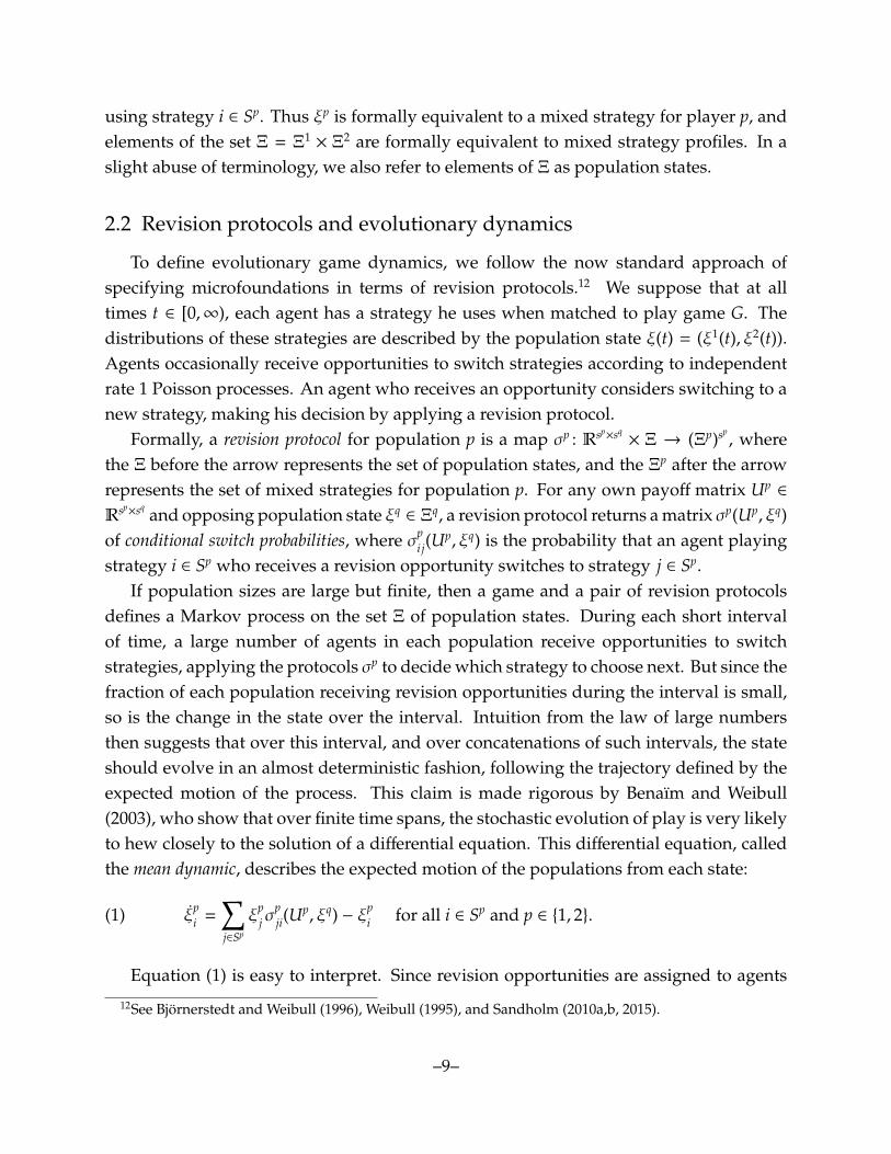
2.2 Revision protocols and evolutionary dynamics

To define evolutionary game dynamics, we follow the now standard approach ofspecifying microfoundations in terms of revision protocols.12 We suppose that at alltimes t ∈ [0,∞), each agent has a strategy he uses when matched to play game G. Thedistributions of these strategies are described by the population state ξ(t) = (ξ1(t), ξ2(t)).Agents occasionally receive opportunities to switch strategies according to independentrate 1 Poisson processes. An agent who receives an opportunity considers switching to anew strategy, making his decision by applying a revision protocol.

Formally, a revision protocol for population p is a map σp : Rsp×sq× Ξ → (Ξp)sp , where

the Ξ before the arrow represents the set of population states, and the Ξp after the arrowrepresents the set of mixed strategies for population p. For any own payoff matrix Up

∈

Rsp×sq and opposing population state ξq

∈ Ξq, a revision protocol returns a matrix σp(Up, ξq)of conditional switch probabilities, where σp

ij(Up, ξq) is the probability that an agent playing

strategy i ∈ Sp who receives a revision opportunity switches to strategy j ∈ Sp.If population sizes are large but finite, then a game and a pair of revision protocols

defines a Markov process on the set Ξ of population states. During each short intervalof time, a large number of agents in each population receive opportunities to switchstrategies, applying the protocols σp to decide which strategy to choose next. But since thefraction of each population receiving revision opportunities during the interval is small,so is the change in the state over the interval. Intuition from the law of large numbersthen suggests that over this interval, and over concatenations of such intervals, the stateshould evolve in an almost deterministic fashion, following the trajectory defined by theexpected motion of the process. This claim is made rigorous by Benaım and Weibull(2003), who show that over finite time spans, the stochastic evolution of play is very likelyto hew closely to the solution of a differential equation. This differential equation, calledthe mean dynamic, describes the expected motion of the populations from each state:

(1) ξpi =

∑j∈Sp

ξpjσ

pji(U

p, ξq) − ξpi for all i ∈ Sp and p ∈ {1, 2}.

Equation (1) is easy to interpret. Since revision opportunities are assigned to agents

12See Bjornerstedt and Weibull (1996), Weibull (1995), and Sandholm (2010a,b, 2015).

–9–

randomly, there is an outflow from each strategy i proportional to its current level ofuse. To generate inflow into i, an agent playing some strategy j must receive a revisionopportunity, and applying his revision protocol must lead him to play strategy i.

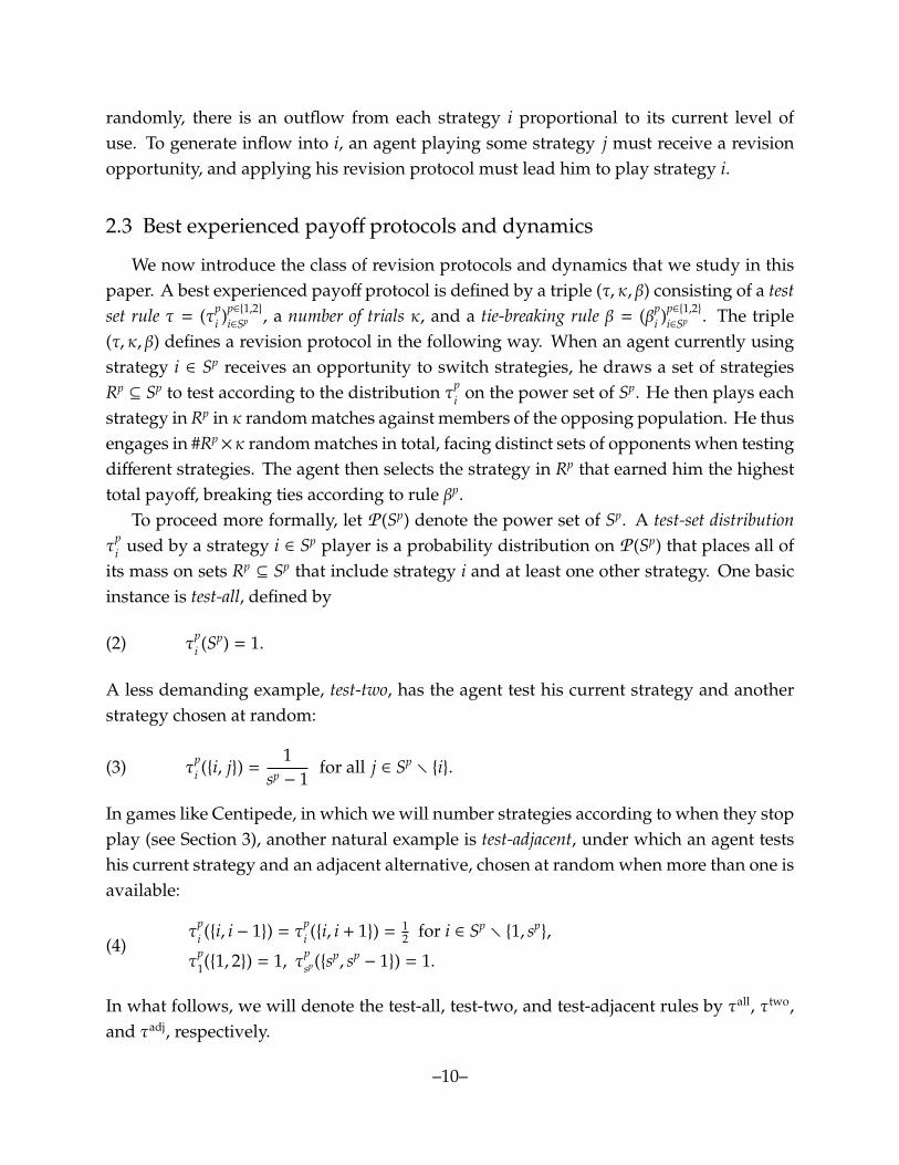
2.3 Best experienced payoff protocols and dynamics

We now introduce the class of revision protocols and dynamics that we study in thispaper. A best experienced payoff protocol is defined by a triple (τ, κ, β) consisting of a testset rule τ = (τp

i )p∈{1,2}i∈Sp , a number of trials κ, and a tie-breaking rule β = (βp

i )p∈{1,2}i∈Sp . The triple

(τ, κ, β) defines a revision protocol in the following way. When an agent currently usingstrategy i ∈ Sp receives an opportunity to switch strategies, he draws a set of strategiesRp⊆ Sp to test according to the distribution τp

i on the power set of Sp. He then plays eachstrategy in Rp in κ random matches against members of the opposing population. He thusengages in #Rp

×κ random matches in total, facing distinct sets of opponents when testingdifferent strategies. The agent then selects the strategy in Rp that earned him the highesttotal payoff, breaking ties according to rule βp.

To proceed more formally, let P (Sp) denote the power set of Sp. A test-set distributionτp

i used by a strategy i ∈ Sp player is a probability distribution on P (Sp) that places all ofits mass on sets Rp

⊆ Sp that include strategy i and at least one other strategy. One basicinstance is test-all, defined by

(2) τpi (Sp) = 1.

A less demanding example, test-two, has the agent test his current strategy and anotherstrategy chosen at random:

(3) τpi ({i, j}) =

1sp − 1

for all j ∈ Sp r {i}.

In games like Centipede, in which we will number strategies according to when they stopplay (see Section 3), another natural example is test-adjacent, under which an agent testshis current strategy and an adjacent alternative, chosen at random when more than one isavailable:

(4)τp

i ({i, i − 1}) = τpi ({i, i + 1}) = 1

2 for i ∈ Sp r {1, sp},

τp1({1, 2}) = 1, τp

sp({sp, sp− 1}) = 1.

In what follows, we will denote the test-all, test-two, and test-adjacent rules by τall, τtwo,and τadj, respectively.

–10–

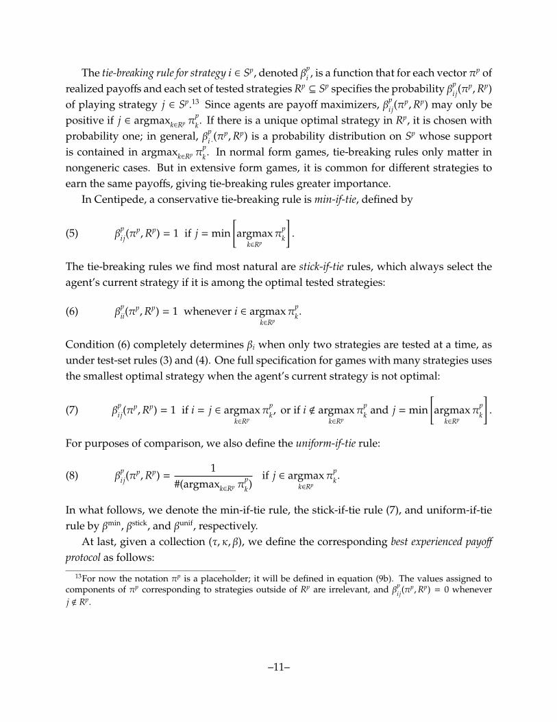
The tie-breaking rule for strategy i ∈ Sp, denoted βpi , is a function that for each vector πp of

realized payoffs and each set of tested strategies Rp⊆ Sp specifies the probability βp

ij(πp,Rp)

of playing strategy j ∈ Sp.13 Since agents are payoff maximizers, βpij(π

p,Rp) may only bepositive if j ∈ argmaxk∈Rp π

pk . If there is a unique optimal strategy in Rp, it is chosen with

probability one; in general, βpi ·(π

p,Rp) is a probability distribution on Sp whose supportis contained in argmaxk∈Rp π

pk . In normal form games, tie-breaking rules only matter in

nongeneric cases. But in extensive form games, it is common for different strategies toearn the same payoffs, giving tie-breaking rules greater importance.

In Centipede, a conservative tie-breaking rule is min-if-tie, defined by

(5) βpij(π

p,Rp) = 1 if j = min[argmax

k∈Rpπp

k

].

The tie-breaking rules we find most natural are stick-if-tie rules, which always select theagent’s current strategy if it is among the optimal tested strategies:

(6) βpii(π

p,Rp) = 1 whenever i ∈ argmaxk∈Rp

πpk .

Condition (6) completely determines βi when only two strategies are tested at a time, asunder test-set rules (3) and (4). One full specification for games with many strategies usesthe smallest optimal strategy when the agent’s current strategy is not optimal:

(7) βpij(π

p,Rp) = 1 if i = j ∈ argmaxk∈Rp

πpk , or if i < argmax

k∈Rpπp

k and j = min[argmax

k∈Rpπp

k

].

For purposes of comparison, we also define the uniform-if-tie rule:

(8) βpij(π

p,Rp) =1

#(argmaxk∈Rp πpk)

if j ∈ argmaxk∈Rp

πpk .

In what follows, we denote the min-if-tie rule, the stick-if-tie rule (7), and uniform-if-tierule by βmin, βstick, and βunif, respectively.

At last, given a collection (τ, κ, β), we define the corresponding best experienced payoffprotocol as follows:

13For now the notation πp is a placeholder; it will be defined in equation (9b). The values assigned tocomponents of πp corresponding to strategies outside of Rp are irrelevant, and βp

ij(πp,Rp) = 0 whenever

j < Rp.

–11–

σpij(U

p, ξq) =∑

Rp⊆Sp

τpi (Rp)

∑r

∏k∈Rp

κ∏m=1

ξqrkm

βpij(π

p(r),Rp)

,(9a)

where πpk(r) =

κ∑m=1

Upkrkm

for all k ∈ Rp,(9b)

where Upk` denotes the payoff of a population p agent who plays k against an opponent

playing `, and where the interior sum in (9a) is taken over all lists r : Rp×{1, . . . , κ} → Sq of

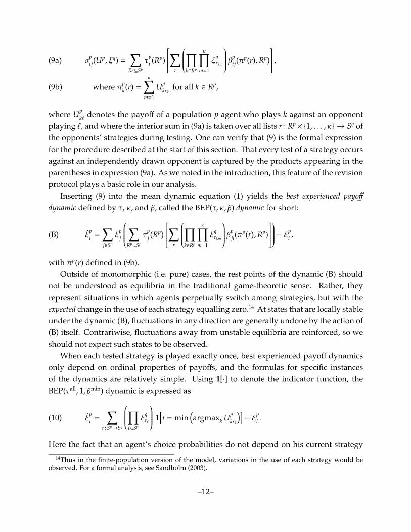
the opponents’ strategies during testing. One can verify that (9) is the formal expressionfor the procedure described at the start of this section. That every test of a strategy occursagainst an independently drawn opponent is captured by the products appearing in theparentheses in expression (9a). As we noted in the introduction, this feature of the revisionprotocol plays a basic role in our analysis.

Inserting (9) into the mean dynamic equation (1) yields the best experienced payoffdynamic defined by τ, κ, and β, called the BEP(τ, κ, β) dynamic for short:

(B) ξpi =

∑j∈Sp

ξpj

∑Rp⊆Sp

τpj (R

p)

∑r

∏k∈Rp

κ∏m=1

ξqrkm

βpji(π

p(r),Rp)

− ξp

i ,

with πp(r) defined in (9b).Outside of monomorphic (i.e. pure) cases, the rest points of the dynamic (B) should

not be understood as equilibria in the traditional game-theoretic sense. Rather, theyrepresent situations in which agents perpetually switch among strategies, but with theexpected change in the use of each strategy equalling zero.14 At states that are locally stableunder the dynamic (B), fluctuations in any direction are generally undone by the action of(B) itself. Contrariwise, fluctuations away from unstable equilibria are reinforced, so weshould not expect such states to be observed.

When each tested strategy is played exactly once, best experienced payoff dynamicsonly depend on ordinal properties of payoffs, and the formulas for specific instancesof the dynamics are relatively simple. Using 1[·] to denote the indicator function, theBEP(τall, 1, βmin) dynamic is expressed as

(10) ξpi =

∑r : Sp→Sq

∏`∈Sp

ξqr`

1[i = min

(argmaxk Up

krk

)]− ξp

i .

Here the fact that an agent’s choice probabilities do not depend on his current strategy

14Thus in the finite-population version of the model, variations in the use of each strategy would beobserved. For a formal analysis, see Sandholm (2003).

–12–

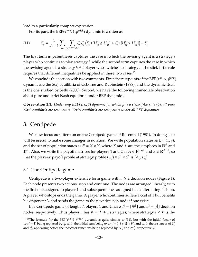
lead to a particularly compact expression.For its part, the BEP(τtwo, 1, βstick) dynamic is written as

(11) ξpi =

1sp − 1

∑h,i

∑(k,`)∈Sq×Sq

ξqk ξ

q`

(ξp

i 1[Upik ≥ Up

h`] + ξph 1[Up

ik > Uph`]

)− ξp

i .

The first term in parentheses captures the case in which the revising agent is a strategy iplayer who continues to play strategy i, while the second term captures the case in whichthe revising agent is a strategy h , i player who switches to strategy i. The stick-if-tie rulerequires that different inequalities be applied in these two cases.15

We conclude this section with two comments. First, the rest points of the BEP(τall, κ, βunif)dynamic are the S(k) equilibria of Osborne and Rubinstein (1998), and the dynamic itselfis the one studied by Sethi (2000). Second, we have the following immediate observationabout pure and strict Nash equilibria under BEP dynamics.

Observation 2.1. Under any BEP(τ, κ, β) dynamic for which β is a stick-if-tie rule (6), all pureNash equilibria are rest points. Strict equilibria are rest points under all BEP dynamics.

3. Centipede

We now focus our attention on the Centipede game of Rosenthal (1981). In doing so itwill be useful to make some changes in notation. We write population states as ξ = (x, y),and the set of population states as Ξ = X × Y, where X and Y are the simplices in Rs1 andRs2 . Also, we write the payoff matrices for players 1 and 2 as A ∈ Rs1

×s2 and B ∈ Rs1×s2 , so

that the players’ payoff profile at strategy profile (i, j) ∈ S1× S2 is (Ai j,Bi j).

3.1 The Centipede game

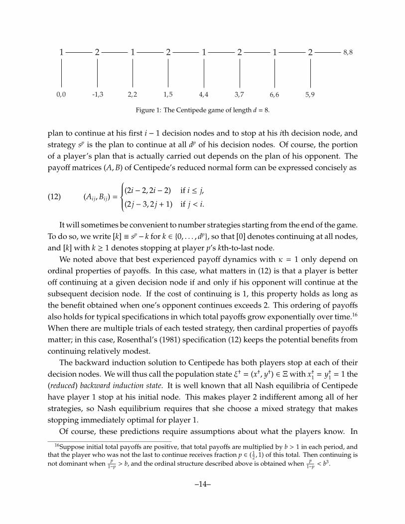
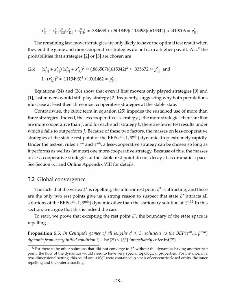
Centipede is a two-player extensive form game with d ≥ 2 decision nodes (Figure 1).Each node presents two actions, stop and continue. The nodes are arranged linearly, withthe first one assigned to player 1 and subsequent ones assigned in an alternating fashion.A player who stops ends the game. A player who continues suffers a cost of 1 but benefitshis opponent 3, and sends the game to the next decision node if one exists.

In a Centipede game of length d, players 1 and 2 have d1 = bd+12 c and d2 = bd

2c decisionnodes, respectively. Thus player p has sp = dp + 1 strategies, where strategy i < sp is the

15The formula for the BEP(τadj, 1, βstick) dynamic is quite similar to (11), but with the initial factor of1/(sp

− 1) being replaced by 12 , with the initial sum being over {i − 1, i + 1} ∩ Sp, and with the instances of ξp

1and ξp

sp appearing before the indicator functions being replaced by 2ξp1 and 2ξp

sp , respectively.

–13–

1

0,0

2

-1,3

1

2,2

2

1,5

1

4,4

8,82

3,7

1

6,6

2

5,9

Figure 1: The Centipede game of length d = 8.

plan to continue at his first i − 1 decision nodes and to stop at his ith decision node, andstrategy sp is the plan to continue at all dp of his decision nodes. Of course, the portionof a player’s plan that is actually carried out depends on the plan of his opponent. Thepayoff matrices (A,B) of Centipede’s reduced normal form can be expressed concisely as

(12) (Ai j,Bi j) =

(2i − 2, 2i − 2) if i ≤ j,

(2 j − 3, 2 j + 1) if j < i.

It will sometimes be convenient to number strategies starting from the end of the game.To do so, we write [k] ≡ sp

− k for k ∈ {0, . . . , dp}, so that [0] denotes continuing at all nodes,

and [k] with k ≥ 1 denotes stopping at player p’s kth-to-last node.We noted above that best experienced payoff dynamics with κ = 1 only depend on

ordinal properties of payoffs. In this case, what matters in (12) is that a player is betteroff continuing at a given decision node if and only if his opponent will continue at thesubsequent decision node. If the cost of continuing is 1, this property holds as long asthe benefit obtained when one’s opponent continues exceeds 2. This ordering of payoffsalso holds for typical specifications in which total payoffs grow exponentially over time.16

When there are multiple trials of each tested strategy, then cardinal properties of payoffsmatter; in this case, Rosenthal’s (1981) specification (12) keeps the potential benefits fromcontinuing relatively modest.

The backward induction solution to Centipede has both players stop at each of theirdecision nodes. We will thus call the population state ξ† = (x†, y†) ∈ Ξ with x†1 = y†1 = 1 the(reduced) backward induction state. It is well known that all Nash equilibria of Centipedehave player 1 stop at his initial node. This makes player 2 indifferent among all of herstrategies, so Nash equilibrium requires that she choose a mixed strategy that makesstopping immediately optimal for player 1.

Of course, these predictions require assumptions about what the players know. In

16Suppose initial total payoffs are positive, that total payoffs are multiplied by b > 1 in each period, andthat the player who was not the last to continue receives fraction p ∈ ( 1

2 , 1) of this total. Then continuing isnot dominant when p

1−p > b, and the ordinal structure described above is obtained when p1−p < b3.

–14–

the traditional justification of Nash equilibrium, players are assumed to correctly an-ticipate opponents’ play. Likewise, traditional justifications of the backward inductionsolution require agents to maintain common belief in rational future play, even if behaviorcontradicting this belief has been observed in the past.17

3.2 Best experienced payoff dynamics for the Centipede game

To obtain explicit formulas for best experienced payoff dynamics in the Centipedegame, we substitute the payoff functions (12) into the general formulas from Section 2and simplify the results. Here we present the two examples from the end of Section2.3. Explicit formulas for the remaining BEP(τ, 1, β) dynamics with τ ∈ {τall, τtwo, τadj

} andβ ∈ {βmin, βstick, βunif

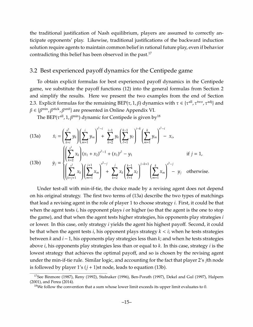
} are presented in Online Appendix VI.The BEP(τall, 1, βmin) dynamic for Centipede is given by18

xi =

s2∑k=i

yk

i∑

m=1

ym

s1−i

+

i−1∑k=2

yk

k−1∑`=1

y`

i−k k∑

m=1

ym

s1−i

− xi,(13a)

y j =

s1∑k=2

xk

(x1 + x2)s2−1 + (x1)s2

− y1 if j = 1, s1∑k= j+1

xk

j+1∑

m=1

xm

s2− j

+

j∑k=2

xk

k−1∑`=1

x`

j−k+1 k∑

m=1

xm

s2− j

− y j otherwise.

(13b)

Under test-all with min-if-tie, the choice made by a revising agent does not dependon his original strategy. The first two terms of (13a) describe the two types of matchingsthat lead a revising agent in the role of player 1 to choose strategy i. First, it could be thatwhen the agent tests i, his opponent plays i or higher (so that the agent is the one to stopthe game), and that when the agent tests higher strategies, his opponents play strategies ior lower. In this case, only strategy i yields the agent his highest payoff. Second, it couldbe that when the agent tests i, his opponent plays strategy k < i; when he tests strategiesbetween k and i− 1, his opponents play strategies less than k; and when he tests strategiesabove i, his opponents play strategies less than or equal to k. In this case, strategy i is thelowest strategy that achieves the optimal payoff, and so is chosen by the revising agentunder the min-if-tie rule. Similar logic, and accounting for the fact that player 2’s jth nodeis followed by player 1’s ( j + 1)st node, leads to equation (13b).

17See Binmore (1987), Reny (1992), Stalnaker (1996), Ben-Porath (1997), Dekel and Gul (1997), Halpern(2001), and Perea (2014).

18We follow the convention that a sum whose lower limit exceeds its upper limit evaluates to 0.

–15–

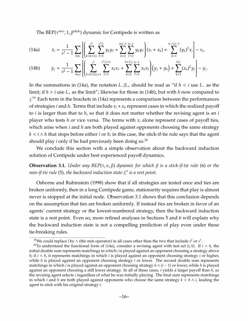
The BEP(τtwo, 1, βstick) dynamic for Centipede is written as

xi =1

s1 − 1

∑h,i

s2∑

k=h+1|i

s2|i∑

`=1

yky` +

h|i−1∑k=2

k−1∑`=1

yky`

(xi + xh) +

h−1|i−1∑k=1

(yk)2xi

− xi,(14a)

y j =1

s2 − 1

∑h, j

s1∑

k=h+2| j+1

s1| j+1∑`=1

xkx` +

h+1| j∑k=2

k−1∑`=1

xkx`

(y j + yh

)+

h| j∑k=1

(xk)2 y j

− y j.(14b)

In the summations in (14a), the notation L− |L+ should be read as “if h < i use L− as thelimit; if h > i use L+ as the limit”; likewise for those in (14b), but with h now compared toj.19 Each term in the brackets in (14a) represents a comparison between the performancesof strategies i and h. Terms that include xi + xh represent cases in which the realized payoff

to i is larger than that to h, so that it does not matter whether the revising agent is an iplayer who tests h or vice versa. The terms with xi alone represent cases of payoff ties,which arise when i and h are both played against opponents choosing the same strategyk < i ∧ h that stops before either i or h; in this case, the stick-if-tie rule says that the agentshould play i only if he had previously been doing so.20

We conclude this section with a simple observation about the backward inductionsolution of Centipede under best experienced payoff dynamics.

Observation 3.1. Under any BEP(τ, κ, β) dynamic for which β is a stick-if-tie rule (6) or themin-if-tie rule (5), the backward induction state ξ† is a rest point.

Osborne and Rubinstein (1998) show that if all strategies are tested once and ties arebroken uniformly, then in a long Centipede game, stationarity requires that play is almostnever is stopped at the initial node. Observation 3.1 shows that this conclusion dependson the assumption that ties are broken uniformly. If instead ties are broken in favor of anagents’ current strategy or the lowest-numbered strategy, then the backward inductionstate is a rest point. Even so, more refined analyses in Sections 5 and 6 will explain whythe backward induction state is not a compelling prediction of play even under thesetie-breaking rules.

19We could replace | by ∧ (the min operator) in all cases other than the two that include s2 or s1.20To understand the functional form of (14a), consider a revising agent with test set {i, h}. If i > h, the

initial double sum represents matchings in which i is played against an opponent choosing a strategy aboveh; if i < h, it represents matchings in which i is played against an opponent choosing strategy i or higher,while h is played against an opponent choosing strategy i or lower. The second double sum representsmatchings in which i is played against an opponent choosing strategy h ∧ (i − 1) or lower, while h is playedagainst an opponent choosing a still lower strategy. In all of these cases, i yields a larger payoff than h, sothe revising agent selects i regardless of what he was initially playing. The final sum represents matchingsin which i and h are both played against opponents who choose the same strategy k < h ∧ i, leading theagent to stick with his original strategy i.

–16–

4. Exact solutions of systems of polynomial equations

An important first step in analyzing a system of differential equations is to identify itsrest points. From this point of view, a key feature of best experienced payoff dynamicsis that they are defined by systems of polynomial equations with rational coefficients. Inwhat follows, we explain the algebraic tools that we use to determine the exact valuesof the components of these rest points. The contents of this section are not needed tounderstand the presentation of our results, which begins in Section 5. Some readers mayprefer to return to this section after reading those that follow.

4.1 Grobner bases

Let Q[z1, . . . , zn], or Q[z] for short, denote the collection (more formally, the ring) ofpolynomials in the variables z1, . . . , zn with rational coefficients. Let F = { f1, . . . fm} ⊂ Q[z]be a set of such polynomials. Let Z be a subset ofRn, and consider the problem of findingthe set of points z∗ ∈ Z that are zeroes of all polynomials in F.

To do so, it is convenient to first consider finding all zeroes in Cn of the polynomials inF. In this case, the set of interest,

(15) V( f1, . . . , fm) = {z∗ ∈ Cn : f j(z∗) = 0 for all 1 ≤ j ≤ m}

is called the variety (or algebraic set) generated by f1, . . . , fm. To characterize (15), it is usefulto introduce the ideal generated by f1, . . . , fm:

(16) 〈 f1, . . . , fm〉 ={∑m

j=1h j f j : h j ∈ C[z] for all 1 ≤ j ≤ m

}.

Thus the ideal (16) is the set of linear combinations of the polynomials f1, . . . , fm, where thecoefficients on each are themselves polynomials in C[z]. It is easy to verify that any othercollection of polynomials in C[z] whose linear combinations generate the ideal (16)—thatis, any other basis for the ideal—also generates the variety (15).

For our purposes, the most useful basis for the ideal (16) is the reduced lex-order Grobnerbasis, which we denote by G ⊂ Q[z]. This basis, which contains no superfluous polyno-mials and is uniquely determined by its ideal and the ordering of the variables, has thisconvenient property: it consists of polynomials in zn only, polynomials in zn and zn−1 only,polynomials in zn, zn−1, and zn−2 only, and so forth. Thus if the variety (15) has cardinality|V| < ∞, then it can be computed sequentially by solving univariate polynomials and

–17–

substituting backward.21

In many cases, including all that arise in this paper, the basis G is of the simple form

(17) G = {gn(zn), zn−1 − gn−1(zn), . . . , z1 − g1(zn)}

for some univariate polynomials gn, . . . , g1, where gn has degree deg(gn) = |V| and wheredeg(gk) < |V| for k < n.22 In such cases, one computes the variety (15) by finding the |V|complex roots of gn, and then substituting each into the other n− 1 polynomials to obtainthe |V| elements of (15).23

4.2 Algebraic numbers

The first step in finding the zeros of the polynomials in G ⊂ Q[z] is to find the roots ofthe univariate polynomial gn. There are well-known limits to what can be accomplishedhere: Abel’s theorem states that there is no solution in radicals to general univariatepolynomial equations of degree five or higher. Nevertheless, tools from computationalalgebra allow us to represent such solutions exactly.

Let Q ⊂ C denote the set of algebraic numbers: the complex numbers that are roots ofpolynomials with rational coefficients. Q is a subfield ofC, and this fact and the definitionof algebraic numbers are summarized by saying that Q is the algebraic closure of Q.24

Every univariate polynomial g ∈ Q[x] can be factored as a product of irreducible poly-nomials inQ[x], which cannot themselves be further factored into products of nonconstantelements of Q[x].25 If an irreducible polynomial h ∈ Q[x] is of degree k, it has k distinctroots a1, . . . , ak ∈ Q. The multiple of h whose leading term has coefficient 1 is called the

21The notion of Grobner bases and the basic algorithm for computing them are due to Buchberger (1965).Cox et al. (2015) provide an excellent current account of Grobner basis algorithms, as well as a thoroughintroduction to the ideas summarized above.

22According to the shape lemma, a sufficient condition for the reduced lex-order basis to be of form (17) isthat each point in (15) have a distinct zn component and that (16) be a radical ideal, meaning that if it includessome integer power of a polynomial, then it includes the polynomial itself. See Becker et al. (1994) andKubler et al. (2014).

23Although we are only interested in elements of the variety (15) that lie in the state space Ξ, the solutionmethods described above only work if (15) has a finite number of solutions in Cn. For some specificationsof the BEP dynamic, the latter property fails, but we are able to circumvent this problem by introducingadditional variables and equations—see Section 6.2.

24Like C, Q is algebraically closed, in that every univariate polynomial with coefficients in Q has a root inQ. It follows from this and the existence of lex-order Grobner bases that when the variety (15) has a finitenumber of elements, the components of its elements are algebraic numbers.

25“Typical” polynomials in Q[x] are irreducible: for instance, the quadratic ax2 + bx + c with a, b, c ∈ Q isonly reducible if

√

b2 − 4ac ∈ Q. By Gauss’s lemma, polynomial factorization in Q[x] is effectively equivalentto polynomial factorization in Z[x]. For an excellent presentation of polynomial factorization algorithms,see von zur Gathen and Gerhard (2013, Ch. 14–16).

–18–

minimal polynomial of these roots. One often works instead with the multiple of h that isprimitive in Z[x], meaning that its coefficients are integers with greatest common divisor1.

Each algebraic number is uniquely identified by its minimal polynomial h and a labelthat distinguishes the roots of h from one another. For instance, one can label eachroot a j ∈ Q with a numerical approximation that is sufficiently accurate to distinguish a j

from the other roots. In computer algebra systems, the algebraic numbers with minimalpolynomial h are represented by pairs consisting of h and an integer in {1, . . . , k} whichranks the roots of h with respect to some ordering; for instance, the lowest integers arecommonly assigned to the real roots of h in increasing order. Just as the symbol

√2 is a

label for the positive solution to x2− 2 = 0, the approach above provides labels for every

algebraic number.26

If the Grobner basis G is of form (17), then we need only look for the roots of theirreducible factors h of the polynomial gn, which are the possible values of xn ∈ Q; thensubstitution into the univariate polynomials gn−1, . . . , g1 determines the correspondingvalues of the other variables. The fact that these latter values are generated from a fixedalgebraic number allows us to work in subfields of Q in which arithmetic operationsare easy to perform. If the minimal polynomial h of α ∈ Q has degree deg(h), then forany polynomial f , one can find a polynomial f ∗ of degree deg( f ∗) < deg(h) such thatf (α) = f ∗(α). It follows that the values of gn−1(α), . . . , g1(α) are all elements of

Q(α) =

deg(h)−1∑

k=0

ak αk : a0, . . . , adeg(h)−1 ∈ Q

⊂ Q,called the field extension of Q generated by α. Straightforward arguments show that therepresentation of elements of Q(α) by sequences of coefficients (a0, . . . , ad) makes additionand multiplication in Q(α) simple to perform. For further details on algebraic numbersand field extensions, we refer the reader to Dummit and Foote (2004, Chapter 13) andCohen (1993, Chapter 4).

4.3 Examples

To illustrate the techniques above, we use them to compute the rest points of theBEP(τ, 1, βmin) dynamic in the Centipede game with d = 3 nodes, where τ is either τtwo

(equation (3)) or τadj (equation (4)). Although s1 = d1 + 1 = 3 and s2 = d2 + 1 = 2, we need

26There are exact methods based on classic theorems of Sturm and Vincent for isolating the real roots ofa polynomial with rational coefficients; see McNamee (2007, Ch. 2 and 3) and Akritas (2010).

–19–

only write down the laws of motion for three components, say x1, x2, and y1, since theremaining components are then given by x3 = 1 − x1 − x2 and y2 = 1 − y1.27

Example 4.1. The BEP(τtwo, 1, βmin) dynamic in Centipede of length d = 3 is

x1 = 12

(y1(x1 + x2) + y1(x1 + x3)

)− x1,

x2 = 12

(y2(x1 + x2) + (y2 + (y1)2)(x2 + x3)

)− x2,(18)

y1 = ((x2 + x3)(x1 + x2) + (x1)2)(y1 + y2) − y1

(see Online Appendix VI). To find the rest points of this system, we substitute x3 = 1−x1−x2

and y2 = 1 − y1 in the right-hand sides of (18) to obtain a system of three equations andthree unknowns. We then compute a Grobner basis of form (17) for the right-hand sidesof (18):

(19)

{3(y1)4

− 8(y1)3 + 13(y1)2− 12y1 + 4, 4x2 + 3(y1)3

− 5(y1)2 + 6y1 − 4,

8x1 − 3(y1)3 + 2(y1)2− 9y1 + 2

}.

The initial quartic in (19) has roots 1, 23 , and (1 ±

√7 i)/2. Of course, only the first two

roots could be components of states in Ξ. Substituting y1 = 1 in the remaining polynomialsin (19) and equating them to 0 yields x1 = 1 and x2 = 0, which with the simplex constraintsgives us the backward induction state ξ†. Substituting y1 = 2

3 instead yields the interiorstate ξ∗ = (x∗, y∗) = ((1

2 ,13 ,

16 ), ( 2

3 ,13 )). This is the complete set of rest points of the dynamic

(18). _

Example 4.2. The BEP(τadj, 1, βmin) dynamic in Centipede of length d = 3 is

x1 = y1(x1 + 12x2) − x1,

x2 =(y2(x1 + 1

2x2) + (y2 + (y1)2)(12x2 + x3)

)− x2,(20)

y1 = ((x2 + x3)(x1 + x2) + (x1)2)(y1 + y2) − y1

We again compute a Grobner basis of form (17):

(21)

{2(y1)6

− 8(y1)5 + 19(y1)4− 29(y1)3 + 28(y1)2

− 16y1 + 4, 2x2 + 2(y1)5− 4(y1)4

+ 7(y1)3− 7(y1)2 + 4y1 − 2, 2x1 − 2(y1)4 + 4(y1)3

− 7(y1)2 + 5y1 − 2}.

27The Grobner basis algorithm sometimes runs faster if all components are retained and the left-handsides of the constraints

∑s1

i=1 xi − 1 = 0 and∑s2

j=1 y j − 1 = 0 are included in the initial set of polynomials. OurMathematica notebook includes both implementations.

–20–

The initial polynomial in (21) has root 1, which again generates the backward inductionstate ξ†. Dividing this polynomial by y1 − 1 yields

2(y1)5− 6(y1)4 + 13(y1)3

− 16(y1)2 + 12y1 − 4,

which is an irreducible quintic. Using the algorithms mentioned above, one can showthat this quintic has one real root, which we designate by y∗1 = Root[2α5

− 6α4 + 13α3−

16α2 + 12α − 4, 1] ≈ .7295, and four complex roots. Substituting y∗1 into the remainingexpressions in (21) and using the simplex constraints, we obtain an exact expression forthe interior rest point ξ∗, whose components are elements of the field extension Q(y∗1);their approximate values are ξ∗ = (x∗, y∗) ≈ ((.5456, .4047, .0497), (.7295, .2705)). _

5. Analysis of test-all, min-if-tie dynamics

In this section and Section 6.1, we analyze BEP(τ, 1, βmin) dynamics in Centipede games,focusing on the tie-breaking rule that is most favorable to backward induction. Beforeproceeding, we review some standard definitions and results from dynamical systemstheory, and follow this with a simple example.

Consider a C1 differential equation ξ = V(ξ) defined on Ξ whose forward solutions{x(t)}t≥0 do not leave Ξ. State ξ∗ is a rest point if V(ξ∗) = 0, so that the unique solutionstarting from ξ∗ is stationary. Rest point ξ∗ is Lyapunov stable if for every neighborhoodO ⊂ Ξ of ξ∗, there exists a neighborhood O′ ⊂ Ξ of ξ∗ such that every forward solution thatstarts in O′ is contained in O. If ξ∗ is not Lyapunov stable it is unstable, and it is repellingif there is a neighborhood O ⊂ Ξ of ξ∗ such that solutions from all initial conditions inO r {ξ∗} leave O.

Rest point ξ∗ is attracting if there is a neighborhood O ⊂ Ξ of ξ∗ such that all solutionsthat start in O converge toξ∗. A state that is Lyapunov stable and attracting is asymptoticallystable. In this case, the maximal (relatively) open set of states from which solutionsconverge to ξ∗ is called the basin of ξ∗. If the basin of ξ∗ contains int(Ξ), we call ξ∗ almostglobally asymptotically stable; if it is Ξ itself, we call ξ∗ globally asymptotically stable.

The C1 function L : O → R+ is a strict Lyapunov function for rest point ξ∗ ∈ O ifL−1(0) = {ξ∗}, and if its time derivative L(ξ) ≡ ∇L(ξ)′V(ξ) is negative on Or {ξ∗}. Standardresults imply that if such a function exists, then ξ∗ is asymptotically stable.28 If L is a strictLyapunov function for ξ∗ with domain O = Ξ r {ξ†} and ξ† is repelling, then ξ∗ is almostglobally asymptotically stable; if the domain is Ξ, then ξ∗ is globally asymptotically stable.

28See, e.g., Sandholm (2010b, Appendix 7.B).

–21–

Example 5.1. As a preliminary, we consider BEP(τ, 1, βmin) dynamics for the Centipedegame of length 2. Since each player has two strategies, all test-set rules τ have revisingagents test both of them. Focusing on the fractions of agents choosing to continue, we canexpress the dynamics as

(22)x2 = y2 − x2,

y2 = x2x1 − y2.

By way of interpretation, a revising agent in population 1 chooses to continue if hisopponent when he tests continue also continues. A revising agent in population 2 choosesto continue if her opponent continues when she tests continue, and her opponent stopswhen she tests stop.29

Writing 1−x2 for x1 in (22) and then solving for the zeroes, we find that the unique restpoint of (22) is the backward induction state: x†2 = y†2 = 0. Moreover, defining the functionL : [0, 1]2

→ R+ by L(x2, y2) = 12 ((x2)2 + (y2)2), we see that L−1(0) = {ξ†} and that

L(x2, y2) = x2x2 + y2 y2 = x2y2 − (x2)2 + y2x2 − y2(x2)2− (y2)2 = −(x2 − y2)2

− y2(x2)2,

which is nonpositive on [0, 1]2 and equals zero only at the backward induction state. SinceL is a strict Lyapunov function for ξ† on Ξ, state ξ† is globally asymptotically stable. _

In light of this example, our analyses of dynamics using the min-if-tie rule βmin willfocus on Centipede games of lengths d ≥ 3. In the remainder of this section we supposethat τ is the test-all rule τall. Section 6.1 considers the test-set rules τtwo and τadj, andSection 6.2 considers the tie-breaking rules βstick and βunif.

5.1 Rest points and local stability

5.1.1 Analytical results

As we know from Observation 3.1, the backward induction state ξ† of the Centipedegame is a rest point of the BEP(τall, 1, βmin) dynamic. Our first result shows that this restpoint is always repelling.

Proposition 5.2. In Centipede games of lengths d ≥ 3, the backward induction state ξ† is repellingunder the BEP(τall, 1, βmin) dynamic.

The proof of Proposition 5.2, which is presented in Appendix A, is based on a somewhatnonstandard linearization argument. While we are directly concerned with the behavior

29Compare the discussion after equation (13) and Example 5.3 below.

–22–

of the BEP dynamics on the state space Ξ, it is useful to view equation (B) as definingdynamics throughout the affine hull aff(Ξ) = {(x, y) ∈ Rs1+s2 :

∑i∈S1 xi =

∑j∈S2 y j = 1}, which

is then invariant under (B). Vectors of motion through aff(Ξ) are elements of the tangentspace TΞ = {(z1, z2) ∈ Rs1+s2 :

∑i∈S1 z1

i =∑

j∈S2 z2j = 0}. Note that TΞ is a subspace of Rs1+s2 ,

and that aff(Ξ) is obtained from TΞ via translation: aff(Ξ) = TΞ + ξ†.A standard linearization argument is enough to prove that ξ† is unstable. Let the

vector field V : aff(Ξ) → TΞ be defined by the right-hand side of (B). To start the proof,we obtain an expression for the derivative matrix DV(ξ†) that holds for any game lengthd. We then derive formulas for the d linearly independent eigenvectors of DV(ξ†) in thesubspace TΞ and for their corresponding eigenvalues. We find that d−1 of the eigenvaluesare negative, and one is positive. The existence of the latter implies that ξ† is unstable.

To prove that ξ† is repelling, we show that the hyperplane through ξ† defined by thespan of the set of d − 1 eigenvectors with negative eigenvalues supports the convex statespace Ξ at state ξ†. Results from dynamical systems theory—specifically, the Hartman-Grobman and stable manifold theorems (Perko (2001, Sec. 2.7–2.8))—then imply that insome neighborhood O ⊂ aff(Ξ) of ξ†, the set of initial conditions from which solutionsconverge to ξ† is disjoint from Ξ r {ξ†}, and that solutions from the remaining initialconditions eventually move away from ξ†.

The following example provides intuition for the instability of the backward inductionstate; the logic is similar in longer games and for other specifications of the dynamics.

Example 5.3. In a Centipede game of length d = 4, writing out display (13) shows that theBEP(τall, 1, βmin) dynamic is described by

x1 = (y1)2− x1, y1 = (x2 + x3)(x1 + x2)2 + (x1)3

− y1,

x2 = (y2 + y3)(y1 + y2) − x2, y2 = x3 + x2x1(x1 + x2) − y2,(23)

x3 = y3 + y2y1 − x3, y3 = x2(x1)2 + x3(x1 + x2) − y3.

The linearization of this system at (x†, y†) has the positive eigenvalue 1 correspondingto eigenvector (z1, z2) = ((−2, 1, 1), (−2, 1, 1)) (see equation (31)). Thus at state (x, y) =

((1 − 2ε, ε, ε), (1 − 2ε, ε, ε)) with ε > 0 small, we have (x, y) ≈ ((−2ε, ε, ε), (−2ε, ε, ε)).To understand why the addition of agents in both populations playing the cooperative

strategies 2 and 3 is self-reinforcing, we build on the discussion following equation (13).Consider, for instance, component y3, which represents the fraction of agents in population2 who continue at both decision nodes. The last expression in (23) says that a revisingpopulation 2 agent switches to strategy 3 if (i) when testing strategy 3 she meets anopponent playing strategy 2, and when testing strategies 1 and 2 she meets opponents

–23–

playing strategy 1, or (ii) when testing strategy 3 she meets an opponent playing strategy3, and when testing strategy 2 she meets an opponent playing strategy 1 or 2. These eventshave total probability ε(1 − ε) + ε(1 − 2ε)2

≈ 2ε. Since there are y3 = ε agents currentlyplaying strategy 3, outflow from this strategy occurs at rate ε. Combining the inflow andoutflow terms shows that y3 ≈ 2ε − ε = ε. Analogous arguments explain the changes inthe values of the other components of the state. _

It may seem surprising that the play of a weakly dominated strategy—continuing bythe last mover at the last decision node—is positively reinforced at an interior populationstate. This is possible because revising agents test each of their strategies against newlydrawn opponents: as just described, a revising population 2 agent will choose to continueat both of her decision nodes if her opponent’s strategy when she tests strategy 3 ismore cooperative than her opponents’ strategies when she tests her own less cooperativestrategies.

If population 2 agents understand that they are playing Centipede, one might appealto the principle of admissibility to argue that they should not choose to continue at theirlast decision node. One can capture this principle in our context by modeling play in thelength d Centipede game using the dynamics we have defined for the length d− 1 game.30

Since the backward induction state is unstable, we next look for attractors to which thedynamics may converge.

Proposition 5.4. For Centipede games of lengths 3 ≤ d ≤ 6, the BEP(τall, 1, βmin) dynamic hasexactly two rest points, ξ† and ξ∗ ∈ int(Ξ). The rest point ξ∗, whose exact components are known,is asymptotically stable.

Our proof that the dynamics considered in the proposition have exactly two rest pointsuses the Grobner basis and algebraic number algorithms presented in Section 4. Exactsolutions can only be obtained for games of length at most 6 because of the computationaldemands of computing the Grobner bases. One indication of these demands is that whend = 6, the univariate polynomial from the Grobner basis is of degree 221.31

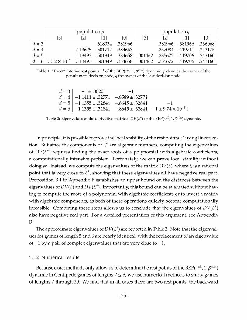
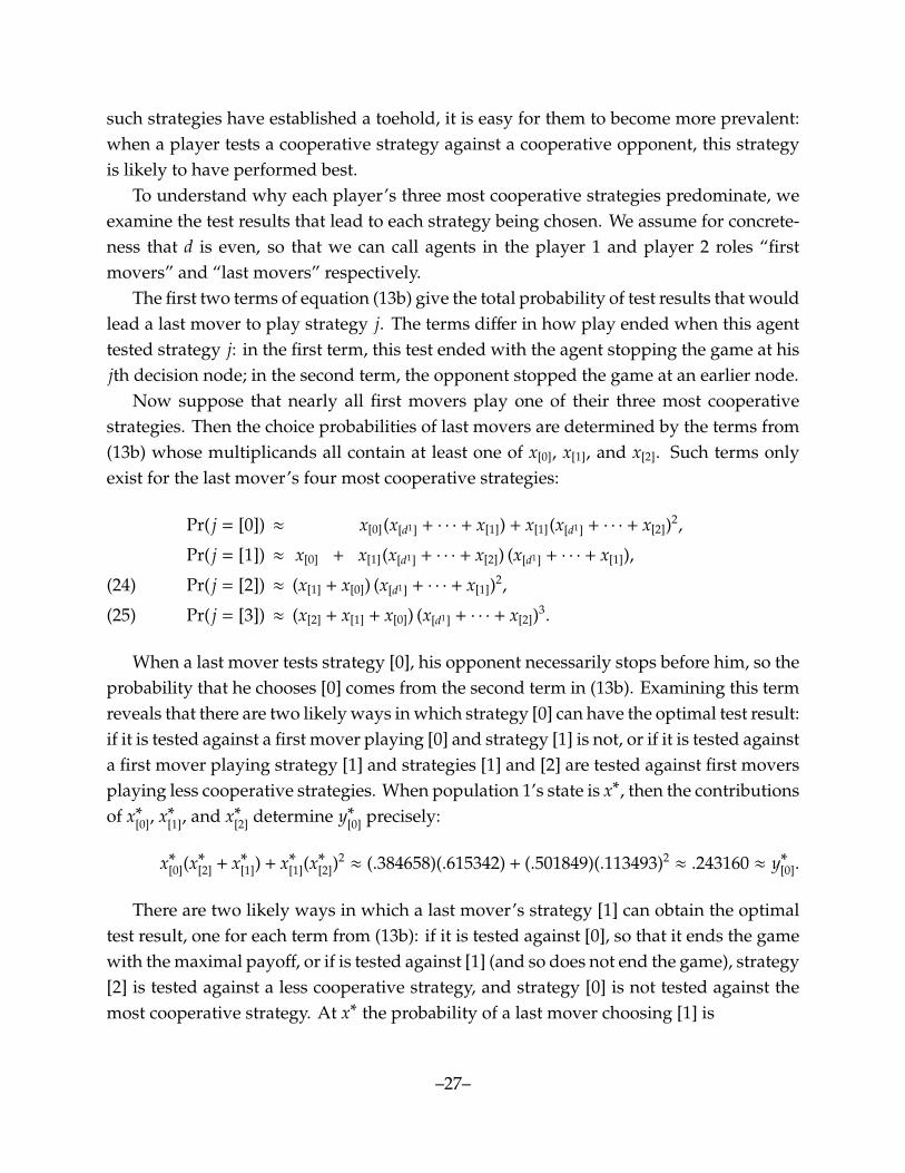
Table 1 reports the approximate values of the interior rest points ξ∗, referring tostrategies using the last-to-first notation [k] introduced in Section 3.1. Evidently, themasses on each strategy are nearly identical for games of lengths 4, 5, and 6, with nearlyall of the weight in both populations being placed on continuing to the end, stopping atthe last node, or stopping at the penultimate node.

30Because of the logical complications inherent in the foundations for iterated admissibility (Samuelson(1992), Brandenburger et al. (2008)), we hesitate to consider iterative truncation of our game dynamics.

31We will see that games of lengths 7 and 8 can be handled for some other choices of τ and β. See Table 7for a summary.

–24–

population p population q[3] [2] [1] [0] [3] [2] [1] [0]

d = 3 .618034 .381966 .381966 .381966 .236068d = 4 .113625 .501712 .384663 .337084 .419741 .243175d = 5 .113493 .501849 .384658 .001462 .335672 .419706 .243160d = 6 3.12 × 10−9 .113493 .501849 .384658 .001462 .335672 .419706 .243160

Table 1: “Exact” interior rest points ξ∗ of the BEP(τall, 1, βmin) dynamic. p denotes the owner of thepenultimate decision node, q the owner of the last decision node.

d = 3 −1 ± .3820 −1d = 4 −1.1411 ± .3277 i −.8589 ± .3277 id = 5 −1.1355 ± .3284 i −.8645 ± .3284 i −1d = 6 −1.1355 ± .3284 i −.8645 ± .3284 i −1 ± 9.74 × 10−5 i

Table 2: Eigenvalues of the derivative matrices DV(ξ∗) of the BEP(τall, 1, βmin) dynamic.

In principle, it is possible to prove the local stability of the rest points ξ∗ using lineariza-tion. But since the components of ξ∗ are algebraic numbers, computing the eigenvaluesof DV(ξ∗) requires finding the exact roots of a polynomial with algebraic coefficients,a computationally intensive problem. Fortunately, we can prove local stability withoutdoing so. Instead, we compute the eigenvalues of the matrix DV(ξ), where ξ is a rationalpoint that is very close to ξ∗, showing that these eigenvalues all have negative real part.Proposition B.1 in Appendix B establishes an upper bound on the distances between theeigenvalues of DV(ξ) and DV(ξ∗). Importantly, this bound can be evaluated without hav-ing to compute the roots of a polynomial with algebraic coefficients or to invert a matrixwith algebraic components, as both of these operations quickly become computationallyinfeasible. Combining these steps allows us to conclude that the eigenvalues of DV(ξ∗)also have negative real part. For a detailed presentation of this argument, see AppendixB.

The approximate eigenvalues of DV(ξ∗) are reported in Table 2. Note that the eigenval-ues for games of length 5 and 6 are nearly identical, with the replacement of an eigenvalueof −1 by a pair of complex eigenvalues that are very close to −1.

5.1.2 Numerical results

Because exact methods only allow us to determine the rest points of the BEP(τall, 1, βmin)dynamic in Centipede games of lengths d ≤ 6, we use numerical methods to study gamesof lengths 7 through 20. We find that in all cases there are two rest points, the backward

–25–

5 10 15 200.0

0.1

0.2

0.3

0.4

0.5

0.6

d

(i) penultimate mover

5 10 15 200.0

0.1

0.2

0.3

0.4

0.5

0.6

d

(ii) last mover

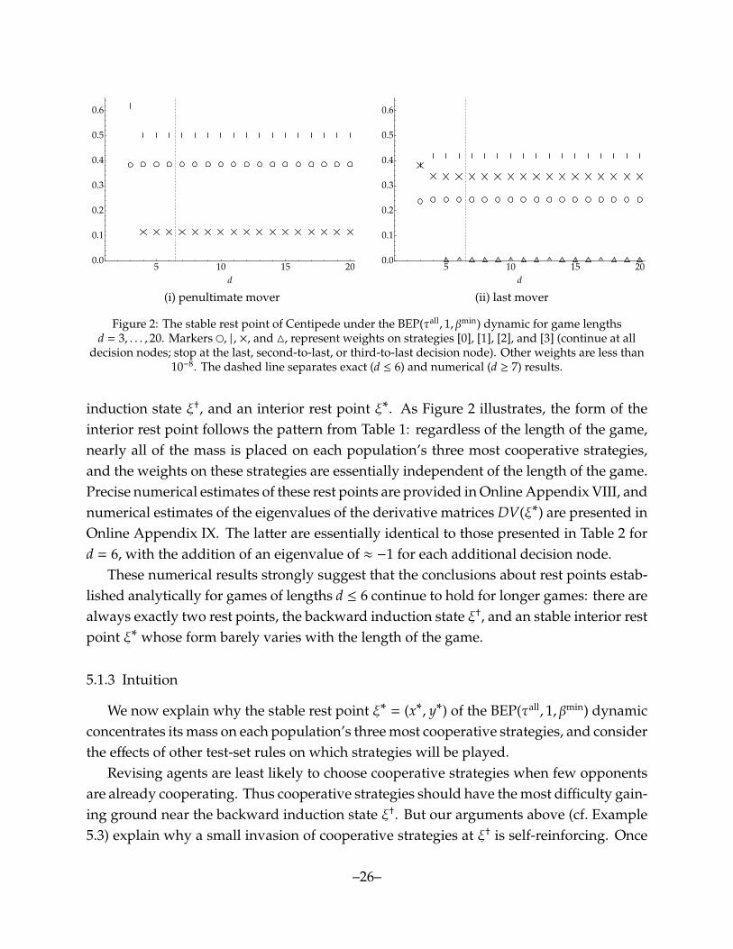
Figure 2: The stable rest point of Centipede under the BEP(τall, 1, βmin) dynamic for game lengthsd = 3, . . . , 20. Markers �, | , ×, and 4, represent weights on strategies [0], [1], [2], and [3] (continue at all

decision nodes; stop at the last, second-to-last, or third-to-last decision node). Other weights are less than10−8. The dashed line separates exact (d ≤ 6) and numerical (d ≥ 7) results.

induction state ξ†, and an interior rest point ξ∗. As Figure 2 illustrates, the form of theinterior rest point follows the pattern from Table 1: regardless of the length of the game,nearly all of the mass is placed on each population’s three most cooperative strategies,and the weights on these strategies are essentially independent of the length of the game.Precise numerical estimates of these rest points are provided in Online Appendix VIII, andnumerical estimates of the eigenvalues of the derivative matrices DV(ξ∗) are presented inOnline Appendix IX. The latter are essentially identical to those presented in Table 2 ford = 6, with the addition of an eigenvalue of ≈ −1 for each additional decision node.

These numerical results strongly suggest that the conclusions about rest points estab-lished analytically for games of lengths d ≤ 6 continue to hold for longer games: there arealways exactly two rest points, the backward induction state ξ†, and an stable interior restpoint ξ∗ whose form barely varies with the length of the game.

5.1.3 Intuition

We now explain why the stable rest point ξ∗ = (x∗, y∗) of the BEP(τall, 1, βmin) dynamicconcentrates its mass on each population’s three most cooperative strategies, and considerthe effects of other test-set rules on which strategies will be played.

Revising agents are least likely to choose cooperative strategies when few opponentsare already cooperating. Thus cooperative strategies should have the most difficulty gain-ing ground near the backward induction state ξ†. But our arguments above (cf. Example5.3) explain why a small invasion of cooperative strategies at ξ† is self-reinforcing. Once

–26–

such strategies have established a toehold, it is easy for them to become more prevalent:when a player tests a cooperative strategy against a cooperative opponent, this strategyis likely to have performed best.

To understand why each player’s three most cooperative strategies predominate, weexamine the test results that lead to each strategy being chosen. We assume for concrete-ness that d is even, so that we can call agents in the player 1 and player 2 roles “firstmovers” and “last movers” respectively.

The first two terms of equation (13b) give the total probability of test results that wouldlead a last mover to play strategy j. The terms differ in how play ended when this agenttested strategy j: in the first term, this test ended with the agent stopping the game at hisjth decision node; in the second term, the opponent stopped the game at an earlier node.

Now suppose that nearly all first movers play one of their three most cooperativestrategies. Then the choice probabilities of last movers are determined by the terms from(13b) whose multiplicands all contain at least one of x[0], x[1], and x[2]. Such terms onlyexist for the last mover’s four most cooperative strategies:

Pr( j = [0]) ≈ x[0](x[d1] + · · · + x[1]) + x[1](x[d1] + · · · + x[2])2,

Pr( j = [1]) ≈ x[0] + x[1](x[d1] + · · · + x[2]) (x[d1] + · · · + x[1]),

Pr( j = [2]) ≈ (x[1] + x[0]) (x[d1] + · · · + x[1])2,(24)

Pr( j = [3]) ≈ (x[2] + x[1] + x[0]) (x[d1] + · · · + x[2])3.(25)

When a last mover tests strategy [0], his opponent necessarily stops before him, so theprobability that he chooses [0] comes from the second term in (13b). Examining this termreveals that there are two likely ways in which strategy [0] can have the optimal test result:if it is tested against a first mover playing [0] and strategy [1] is not, or if it is tested againsta first mover playing strategy [1] and strategies [1] and [2] are tested against first moversplaying less cooperative strategies. When population 1’s state is x∗, then the contributionsof x∗[0], x∗[1], and x∗[2] determine y∗[0] precisely:

x∗[0](x∗[2] + x∗[1]) + x∗[1](x

∗[2])

2≈ (.384658)(.615342) + (.501849)(.113493)2

≈ .243160 ≈ y∗[0].

There are two likely ways in which a last mover’s strategy [1] can obtain the optimaltest result, one for each term from (13b): if it is tested against [0], so that it ends the gamewith the maximal payoff, or if is tested against [1] (and so does not end the game), strategy[2] is tested against a less cooperative strategy, and strategy [0] is not tested against themost cooperative strategy. At x∗ the probability of a last mover choosing [1] is

–27–

x∗[0] + x∗[1]x∗[2](x∗[2] + x∗[1]) ≈ .384658 + (.501849)(.113493)(.615342) ≈ .419706 ≈ y∗[1].

The remaining last-mover strategies are only likely to have the optimal test result whenthey end the game and more cooperative strategies do not earn a higher payoff. At x∗ theprobabilities that strategies [2] or [3] are chosen are

(x∗[1] + x∗[0]) (x∗[2] + x∗[1])2≈ (.886507)(.615342)2

≈ .335672 ≈ y∗[2] and(26)

1 · (x∗[2])3≈ (.113493)3

≈ .001462 ≈ y∗[3].

Equations (24) and (26) show that even if first movers only played strategies [0] and[1], last movers would still play strategy [2] frequently, suggesting why both populationsmust use at least their three most cooperative strategies at the stable state.

Contrariwise, the cubic term in equation (25) impedes the sustained use of more thanthree strategies. Indeed, the less cooperative is strategy j, the more strategies there are thatare more cooperative than j, and for each such strategy k, there are fewer test results underwhich k fails to outperform j. Because of these two factors, the masses on less-cooperativestrategies at the stable rest point of the BEP(τall, 1, βmin) dynamic drop extremely rapidly.Under the test-set rules τtwo and τadj, a less-cooperative strategy can be chosen so long asit performs as well as (at most) one more-cooperative strategy. Because of this, the masseson less-cooperative strategies at the stable rest point do not decay at as dramatic a pace.See Section 6.1 and Online Appendix VIII for details.

5.2 Global convergence

The facts that the vertex ξ† is repelling, the interior rest point ξ∗ is attracting, and theseare the only two rest points give us a strong reason to suspect that state ξ∗ attracts allsolutions of the BEP(τall, 1, βmin) dynamic other than the stationary solution at ξ†.32 In thissection, we argue that this is indeed the case.

To start, we prove that excepting the rest point ξ†, the boundary of the state space isrepelling.

Proposition 5.5. In Centipede games of all lengths d ≥ 3, solutions to the BEP(τall, 1, βmin)dynamic from every initial condition ξ ∈ bd(Ξ) r {ξ†} immediately enter int(Ξ).

32For there to be other solutions that did not converge to ξ∗ without the dynamics having another restpoint, the flow of the dynamics would need to have very special topological properties. For instance, in atwo-dimensional setting, this could occur if ξ∗ were contained in a pair of concentric closed orbits, the innerrepelling and the outer attracting.

–28–

Of course, since the rest point ξ∗ is very close to the boundary for even moderate gamelengths d, the distance of motion from the boundary from some initial conditions must bevery small.

The proof of Proposition 5.5, which is presented in Appendix C, starts with a simpledifferential inequality (Lemma C.1) that lets us obtain explicit positive lower bounds onthe use of any initially unused strategy i at times t ∈ (0,T]. The bounds are given in termsof the probabilities of test results that lead i to be chosen, and thus, backing up one step,in terms of the usage levels of the opponents’ strategies occurring in those tests (equation(63)). With this preliminary result in hand, we prove inward motion from ξ , ξ† byconstructing a sequence that contains all unused strategies, and whose kth strategy couldbe chosen by a revising agent after a test result that only includes strategies that wereinitially in use or that appeared earlier in the sequence. Variations on this argumentestablish inward motion for all other BEP dynamics we consider (Remark C.2).

To argue thatξ∗ is almost globally stable we introduce the candidate Lyapunov function

(27) L(x, y) =

s1∑i=2

(xi − x∗i )2 +

s2∑j=2

(y j − y∗j )2.

In words, L(x, y) is the squared Euclidean distance of (x, y) from (x∗, y∗) if the points in thestate space Ξ are represented in Rd by omitting the first components of x and y.

The Grobner basis techniques from Section 4 do not allow for inequality constraints—here, the nonnegativity constraints on the components of the state—and so are not suitablefor establishing that L is a Lyapunov function.33 We therefore evaluate this claim numeri-cally. For games of lengths 4 through 20, we chose one billion (109) points from the statespace Ξ uniformly at random, and evaluated a floating-point approximation of L at eachpoint. In all instances, the approximate version of L evaluated to a negative number. Thisnumerical procedure covers the state space fairly thoroughly for the game lengths weconsider,34 and so provides strong numerical evidence that the interior rest point ξ∗ is analmost global attractor, and also about the global structure of the dynamics.

33In principle, we could verify that L is a Lyapunov function using an algorithm from real algebraic ge-ometry called cylindrical algebraic decomposition (Collins (1975)), but exact implementations of this algorithmfail to terminate once the dimension of the state space exceeds 2.

34By a standard combinatoric formula, the number of states in a grid in Ξ = X × Y with mesh 1m is(m+s1

−1m

)(m+s2−1

m). Applying this formula shows for a game of length 10, 109 is between the numbers of states

in grids in Ξ of meshes 117 (since

(2217)2

= 693,479,556) and 118 (since

(2318)2

= 1,132,255,201). For a game of length15, the comparable meshes are 1

10 and 111 , and for length 20, 1

7 and 18 .

–29–

6. Analyses of other test-set and tie-breaking rules

6.1 Other test-set rules

We have focused on tie-breaking rule βmin because it is the most favorable to thebackward induction states. On the contrary, the test-set rule τall works in favor of theemergence of cooperative behavior. A revising agent who tests all of his strategies hasmany opportunities to test a cooperative strategy against a cooperative opponent, and soto obtain a high payoff. By reducing the number of such chances, testing fewer strategiesmakes switches to cooperative strategies considerably less likely, especially starting frominitial states with little cooperative play. This leads us to consider BEP dynamics based onthe test-two and test-adjacent rules. In summary, we find that the qualitative predictionsdescribed in the previous section go largely unchanged when these less ambitious test-setrules are used. The conclusion for the test-adjacent rule is particularly striking, as it showsthat cooperative play will emerge even if it only may do so one step at a time.

6.1.1 Test-two

Our analytical results for the BEP(τtwo, 1, βmin) dynamic are as follows

Proposition 6.1. Consider the BEP(τtwo, 1, βmin) dynamic in Centipede games.(i) For games of all lengths d, the rest point ξ† is a repellor.(ii) For games of lengths 3 ≤ d ≤ 8, the dynamic has exactly two rest points, ξ† and ξ∗ ∈ int(Ξ).

The rest point ξ∗ is asymptotically stable.(iii) For games of all lengths d, solutions from every initial condition ξ ∈ bd(Ξ) r {ξ†} imme-

diately enter int(Ξ).

The only differences between the conclusions stated in Proposition 6.1 and those fromthe previous section appears in part (ii): because testing only two strategies leads thepolynomials that define the dynamics to have fewer terms, we are able to analyticallycharacterize the rest points for games of lengths up to d = 8.

The proof that ξ† is a repellor is presented in Appendix A.2. The approach is thatdescribed in Section 5.1.1, but in this case the characterization of the eigenvectors ofDV(ξ†) is more difficult. The characterization of the rest points is again proved using thealgebraic methods from Section 4.

Analogues of the numerical results from Section 5 also go through. As shown in Figure3, the form of the stable rest point settles down once d = 8, with the interior rest point ξ∗

here concentrating its mass on the penultimate player’s four most cooperative strategiesand the last player’s five most cooperative strategies. Online Appendices VIII and IX

–30–

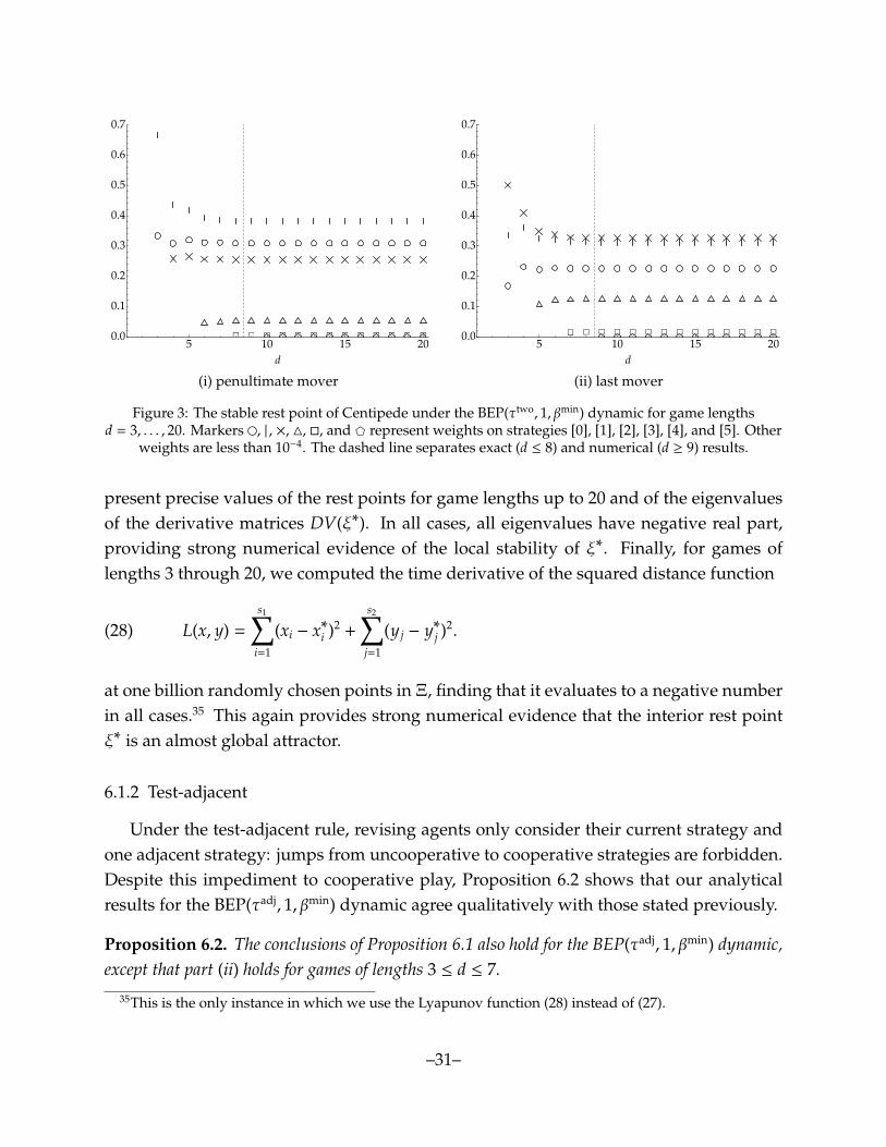
□ □ □ □ □ □ □ □ □ □ □ □ □5 10 15 20

0.0

0.1

0.2

0.3

0.4

0.5

0.6

0.7

d

(i) penultimate mover

□ □ □ □ □ □ □ □ □ □ □ □ □ □

5 10 15 200.0

0.1

0.2

0.3

0.4

0.5

0.6

0.7

d

(ii) last mover

Figure 3: The stable rest point of Centipede under the BEP(τtwo, 1, βmin) dynamic for game lengthsd = 3, . . . , 20. Markers �, | , ×, 4, �, and D represent weights on strategies [0], [1], [2], [3], [4], and [5]. Other

weights are less than 10−4. The dashed line separates exact (d ≤ 8) and numerical (d ≥ 9) results.

present precise values of the rest points for game lengths up to 20 and of the eigenvaluesof the derivative matrices DV(ξ∗). In all cases, all eigenvalues have negative real part,providing strong numerical evidence of the local stability of ξ∗. Finally, for games oflengths 3 through 20, we computed the time derivative of the squared distance function

(28) L(x, y) =

s1∑i=1

(xi − x∗i )2 +

s2∑j=1

(y j − y∗j )2.

at one billion randomly chosen points in Ξ, finding that it evaluates to a negative numberin all cases.35 This again provides strong numerical evidence that the interior rest pointξ∗ is an almost global attractor.

6.1.2 Test-adjacent

Under the test-adjacent rule, revising agents only consider their current strategy andone adjacent strategy: jumps from uncooperative to cooperative strategies are forbidden.Despite this impediment to cooperative play, Proposition 6.2 shows that our analyticalresults for the BEP(τadj, 1, βmin) dynamic agree qualitatively with those stated previously.

Proposition 6.2. The conclusions of Proposition 6.1 also hold for the BEP(τadj, 1, βmin) dynamic,except that part (ii) holds for games of lengths 3 ≤ d ≤ 7.

35This is the only instance in which we use the Lyapunov function (28) instead of (27).

–31–

□□

□ □ □ □ □ □ □ □ □ □ □

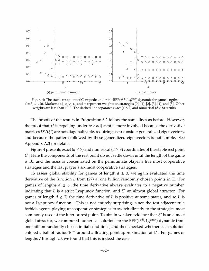
5 10 15 200.0

0.1

0.2

0.3

0.4

0.5

0.6

0.7

d

(i) penultimate mover

□

□

□ □ □ □ □ □ □ □ □ □ □ □

5 10 15 200.0

0.1

0.2

0.3

0.4

0.5

0.6

0.7

d

(ii) last mover

Figure 4: The stable rest point of Centipede under the BEP(τadj, 1, βmin) dynamic for game lengthsd = 3, . . . , 20. Markers �, | , ×, 4, �, and D represent weights on strategies [0], [1], [2], [3], [4], and [5]. Other

weights are less than 10−5. The dashed line separates exact (d ≤ 7) and numerical (d ≥ 8) results.

The proofs of the results in Proposition 6.2 follow the same lines as before. However,the proof that x† is repelling under test-adjacent is more involved because the derivativematrices DV(ξ†) are not diagonalizable, requiring us to consider generalized eigenvectors,and because the pattern followed by these generalized eigenvectors is not simple. SeeAppendix A.3 for details.

Figure 4 presents exact (d ≤ 7) and numerical (d ≥ 8) coordinates of the stable rest pointξ∗. Here the components of the rest point do not settle down until the length of the gameis 10, and the mass is concentrated on the penultimate player’s five most cooperativestrategies and the last player’s six most cooperative strategies.

To assess global stability for games of length d ≥ 3, we again evaluated the timederivative of the function L from (27) at one billion randomly chosen points in Ξ. Forgames of lengths d ≤ 6, the time derivative always evaluates to a negative number,indicating that L is a strict Lyapunov function, and ξ∗ an almost global attractor. Forgames of length d ≥ 7, the time derivative of L is positive at some states, and so L isnot a Lyapunov function. This is not entirely surprising, since the test-adjacent ruleforbids agents playing uncooperative strategies to switch directly to the strategies mostcommonly used at the interior rest point. To obtain weaker evidence that ξ∗ is an almostglobal attractor, we computed numerical solutions to the BEP(τadj, 1, βmin) dynamic fromone million randomly chosen initial conditions, and then checked whether each solutionentered a ball of radius 10−4 around a floating-point approximation of ξ∗. For games oflengths 7 through 20, we found that this is indeed the case.

–32–

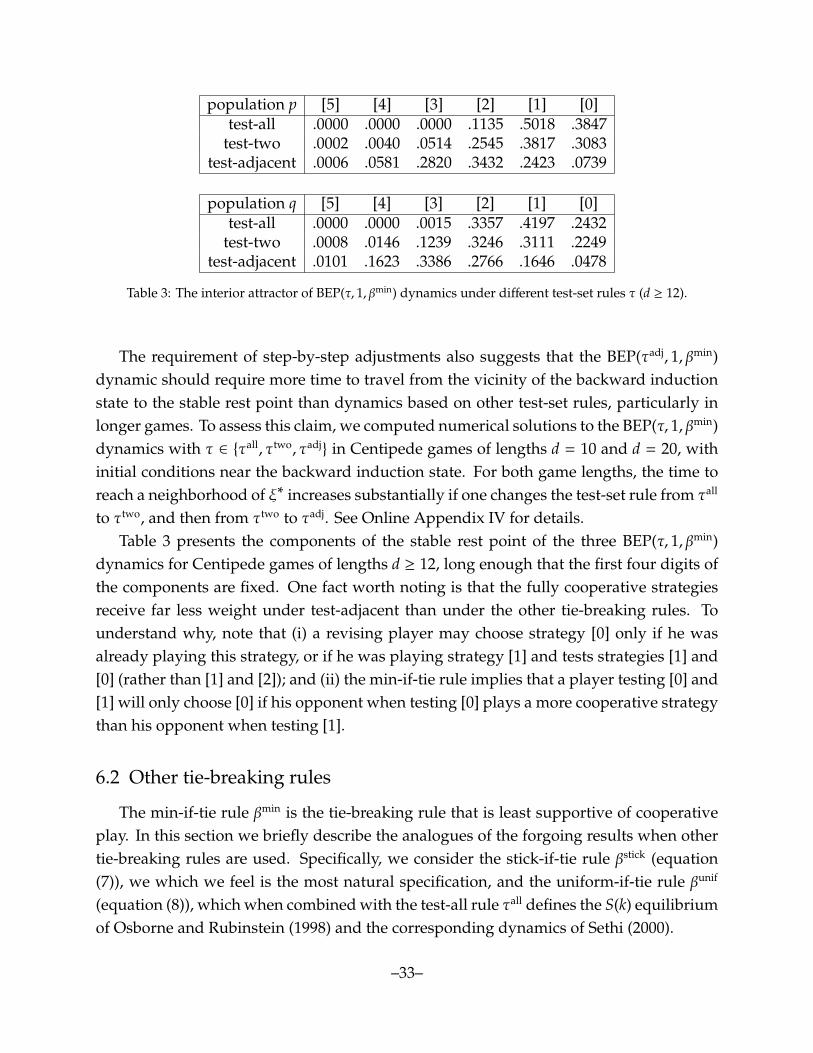
population p [5] [4] [3] [2] [1] [0]test-all .0000 .0000 .0000 .1135 .5018 .3847

test-two .0002 .0040 .0514 .2545 .3817 .3083test-adjacent .0006 .0581 .2820 .3432 .2423 .0739

population q [5] [4] [3] [2] [1] [0]test-all .0000 .0000 .0015 .3357 .4197 .2432

test-two .0008 .0146 .1239 .3246 .3111 .2249test-adjacent .0101 .1623 .3386 .2766 .1646 .0478

Table 3: The interior attractor of BEP(τ, 1, βmin) dynamics under different test-set rules τ (d ≥ 12).

The requirement of step-by-step adjustments also suggests that the BEP(τadj, 1, βmin)dynamic should require more time to travel from the vicinity of the backward inductionstate to the stable rest point than dynamics based on other test-set rules, particularly inlonger games. To assess this claim, we computed numerical solutions to the BEP(τ, 1, βmin)dynamics with τ ∈ {τall, τtwo, τadj

} in Centipede games of lengths d = 10 and d = 20, withinitial conditions near the backward induction state. For both game lengths, the time toreach a neighborhood of ξ∗ increases substantially if one changes the test-set rule from τall

to τtwo, and then from τtwo to τadj. See Online Appendix IV for details.Table 3 presents the components of the stable rest point of the three BEP(τ, 1, βmin)

dynamics for Centipede games of lengths d ≥ 12, long enough that the first four digits ofthe components are fixed. One fact worth noting is that the fully cooperative strategiesreceive far less weight under test-adjacent than under the other tie-breaking rules. Tounderstand why, note that (i) a revising player may choose strategy [0] only if he wasalready playing this strategy, or if he was playing strategy [1] and tests strategies [1] and[0] (rather than [1] and [2]); and (ii) the min-if-tie rule implies that a player testing [0] and[1] will only choose [0] if his opponent when testing [0] plays a more cooperative strategythan his opponent when testing [1].

6.2 Other tie-breaking rules

The min-if-tie rule βmin is the tie-breaking rule that is least supportive of cooperativeplay. In this section we briefly describe the analogues of the forgoing results when othertie-breaking rules are used. Specifically, we consider the stick-if-tie rule βstick (equation(7)), we which we feel is the most natural specification, and the uniform-if-tie rule βunif

(equation (8)), which when combined with the test-all rule τall defines the S(k) equilibriumof Osborne and Rubinstein (1998) and the corresponding dynamics of Sethi (2000).

–33–

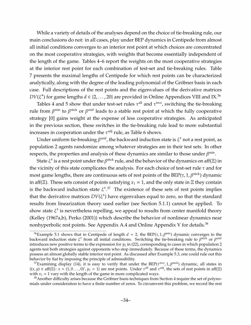
While a variety of details of the analyses depend on the choice of tie-breaking rule, ourmain conclusions do not: in all cases, play under BEP dynamics in Centipede from almostall initial conditions converges to an interior rest point at which choices are concentratedon the most cooperative strategies, with weights that become essentially independent ofthe length of the game. Tables 4–6 report the weights on the most cooperative strategiesat the interior rest point for each combination of test-set and tie-breaking rules. Table7 presents the maximal lengths of Centipede for which rest points can be characterizedanalytically, along with the degree of the leading polynomial of the Grobner basis in eachcase. Full descriptions of the rest points and the eigenvalues of the derivative matricesDV(ξ∗) for game lengths d ∈ {2, . . . , 20} are provided in Online Appendices VIII and IX.36

Tables 4 and 5 show that under test-set rules τall and τtwo, switching the tie-breakingrule from βmin to βstick or βunif leads to a stable rest point at which the fully cooperativestrategy [0] gains weight at the expense of less cooperative strategies. As anticipatedin the previous section, these switches in the tie-breaking rule lead to more substantialincreases in cooperation under the τadj rule, as Table 6 shows.

Under uniform tie-breaking βunif, the backward induction state is ξ† not a rest point, aspopulation 2 agents randomize among whatever strategies are in their test sets. In otherrespects, the properties and analysis of these dynamics are similar to those under βmin.

State ξ† is a rest point under the βstick rule, and the behavior of the dynamics on aff(Ξ) inthe vicinity of this state complicates the analysis. For each choice of test-set rule τ and formost game lengths, there are continuous sets of rest points of the BEP(τ, 1, βstick) dynamicin aff(Ξ). These sets consist of points satisfying x1 = 1, and the only state in Ξ they containis the backward induction state ξ†.37 The existence of these sets of rest points impliesthat the derivative matrices DV(ξ†) have eigenvalues equal to zero, so that the standardresults from linearization theory used earlier (see Section 5.1.1) cannot be applied. Toshow state ξ† is nevertheless repelling, we appeal to results from center manifold theory(Kelley (1967a,b), Perko (2001)) which describe the behavior of nonlinear dynamics nearnonhyperbolic rest points. See Appendix A.4 and Online Appendix V for details.38

36Example 5.1 shows that in Centipede of length d = 2, the BEP(τ, 1, βmin) dynamic converges to thebackward induction state ξ† from all initial conditions. Switching the tie-breaking rule to βstick or βunif

introduces new positive terms to the expression for y2 in (22), corresponding to cases in which population 2agents test both strategies against opponents who stop immediately. Because of these terms, the dynamicspossess an almost globally stable interior rest point. As discussed after Example 5.3, one could rule out thisbehavior by fiat by imposing the principle of admissibility.

37Examining display (14), it is easy to verify that under the BEP(τtwo, 1, βstick) dynamic, all states in{(x, y) ∈ aff(Ξ) : x = (1, 0 . . . , 0)′, y1 = 1} are rest points. Under τall and τadj, the sets of rest points in aff(Ξ)with x1 = 1 vary with the length of the game in more complicated ways.

38Another difficulty arises because the Grobner basis techniques from Section 4 require the set of polyno-mials under consideration to have a finite number of zeros. To circumvent this problem, we record the rest

–34–

population p population q[3] [2] [1] [0] [3] [2] [1] [0]

min .0000 .1135 .5018 .3847 .0015 .3357 .4197 .2432stick/min .0000 .1106 .4999 .3895 .0014 .3315 .4163 .2508uniform .0000 .1080 .4980 .3939 .0013 .3277 .4131 .2580

Table 4: The interior attractor of BEP(τall, 1, β) under different tie-breaking rules β (d ≥ 6). p denotes theowner of the penultimate decision node, q the owner of the last decision node.

population p [5] [4] [3] [2] [1] [0]min .0002 .0040 .0514 .2545 .3817 .3083stick .0001 .0033 .0436 .2256 .3707 .3566

uniform .0001 .0034 .0439 .2261 .3690 .3575

population q [5] [4] [3] [2] [1] [0]min .0008 .0146 .1239 .3246 .3111 .2249stick .0007 .0123 .1066 .2969 .3149 .2685

uniform .0007 .0124 .1071 .2960 .3124 .2713

Table 5: The interior attractor of BEP(τtwo, 1, β) under different tie-breaking rules β (d ≥ 12).

population p [5] [4] [3] [2] [1] [0]min .0006 .0581 .2820 .3432 .2423 .0739stick .0000 .0047 .1253 .3417 .3672 .1611

uniform .0000 .0042 .1200 .3393 .3708 .1658

population q [5] [4] [3] [2] [1] [0]min .0101 .1623 .3386 .2766 .1646 .0478stick .0002 .0360 .2419 .3375 .2623 .1222

uniform .0001 .0333 .2362 .3348 .2685 .1271

Table 6: The interior attractor of BEP(τadj, 1, β) under different tie-breaking rules β (d ≥ 12).

test-all test-two test-adjacentmin 6 (221) 8 (97) 7 (202)stick 5 (65) 8 (128) 6 (47)

uniform 6 (168) 8 (128) 7 (230)

Table 7: The maximal lengths d of Centipede for which the rest points of the BEP(τ, κ, β) dynamic have beencomputed analytically, and the degrees of the leading polynomial of the Grobner basis (in parentheses).

–35–

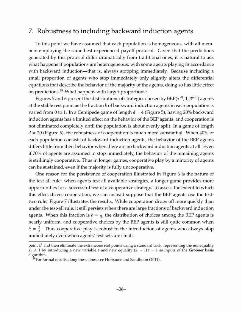
7. Robustness to including backward induction agents

To this point we have assumed that each population is homogeneous, with all mem-bers employing the same best experienced payoff protocol. Given that the predictionsgenerated by this protocol differ dramatically from traditional ones, it is natural to askwhat happens if populations are heterogeneous, with some agents playing in accordancewith backward induction—that is, always stopping immediately. Because including asmall proportion of agents who stop immediately only slightly alters the differentialequations that describe the behavior of the majority of the agents, doing so has little effecton predictions.39 What happens with larger proportions?

Figures 5 and 6 present the distributions of strategies chosen by BEP(τall, 1, βmin) agentsat the stable rest point as the fraction b of backward induction agents in each population isvaried from 0 to 1. In a Centipede game of length d = 4 (Figure 5), having 20% backwardinduction agents has a limited effect on the behavior of the BEP agents, and cooperation isnot eliminated completely until the population is about evenly split. In a game of lengthd = 20 (Figure 6), the robustness of cooperation is much more substantial. When 40% ofeach population consists of backward induction agents, the behavior of the BEP agentsdiffers little from their behavior when there are no backward induction agents at all. Evenif 70% of agents are assumed to stop immediately, the behavior of the remaining agentsis strikingly cooperative. Thus in longer games, cooperative play by a minority of agentscan be sustained, even if the majority is fully uncooperative.

One reason for the persistence of cooperation illustrated in Figure 6 is the nature ofthe test-all rule: when agents test all available strategies, a longer game provides moreopportunities for a successful test of a cooperative strategy. To assess the extent to whichthis effect drives cooperation, we can instead suppose that the BEP agents use the test-two rule. Figure 7 illustrates the results. While cooperation drops off more quickly thanunder the test-all rule, it still persists when there are large fractions of backward inductionagents. When this fraction is b = 1

3 , the distribution of choices among the BEP agents isnearly uniform, and cooperative choices by the BEP agents is still quite common whenb = 2

3 . Thus cooperative play is robust to the introduction of agents who always stopimmediately even when agents’ test sets are small.

point ξ† and then eliminate the extraneous rest points using a standard trick, representing the nonequalityx1 , 1 by introducing a new variable z and new equality (x1 − 1) z = 1 as inputs of the Grobner basisalgorithm.

39For formal results along these lines, see Hofbauer and Sandholm (2011).

–36–

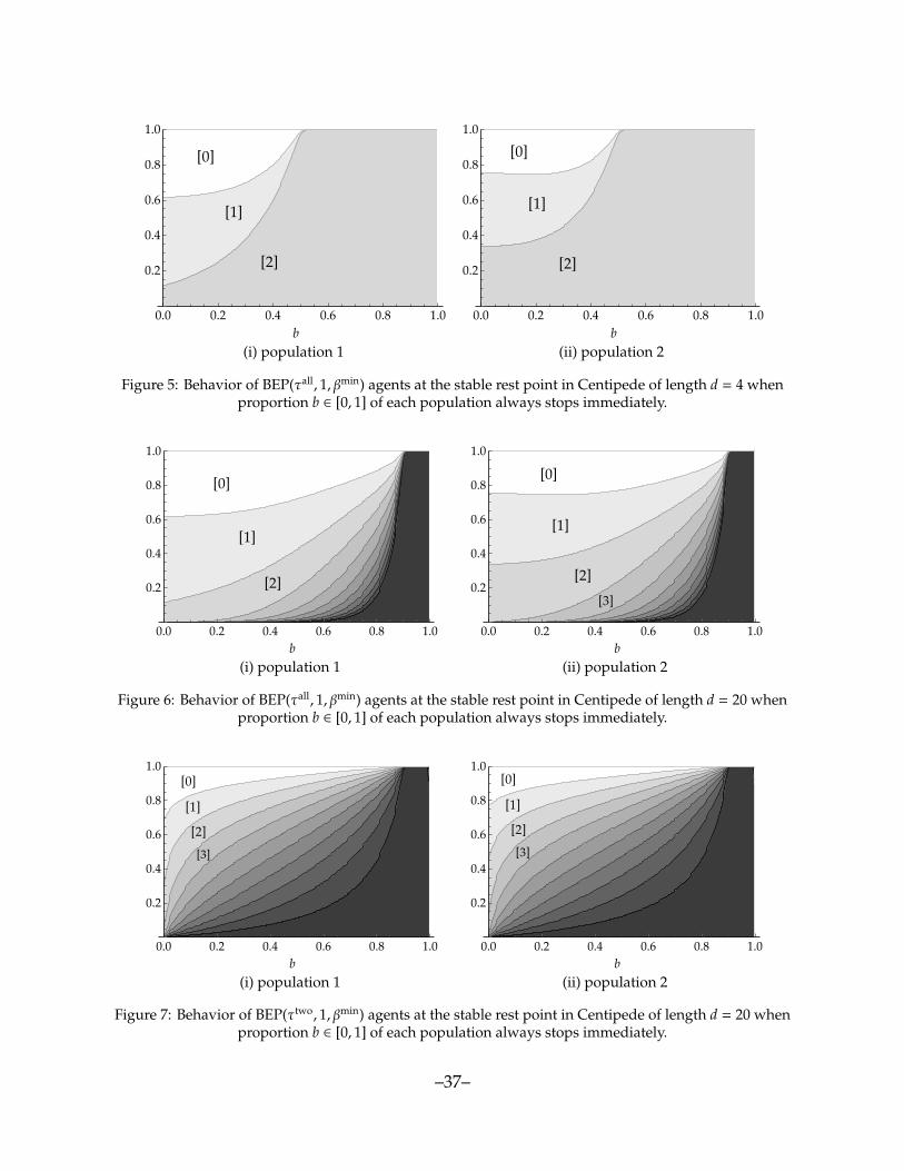
0.0 0.2 0.4 0.6 0.8 1.0

0.2

0.4

0.6

0.8

1.0

b

[0]

[1]

[2]

(i) population 1

0.0 0.2 0.4 0.6 0.8 1.0

0.2

0.4

0.6

0.8

1.0

b

[0]

[1]

[2]

(ii) population 2

Figure 5: Behavior of BEP(τall, 1, βmin) agents at the stable rest point in Centipede of length d = 4 whenproportion b ∈ [0, 1] of each population always stops immediately.

0.0 0.2 0.4 0.6 0.8 1.0

0.2

0.4

0.6

0.8

1.0

b

[0]

[1]

[2]

(i) population 1

0.0 0.2 0.4 0.6 0.8 1.0

0.2

0.4

0.6

0.8

1.0

b

[0]

[1]

[2][3]

(ii) population 2

Figure 6: Behavior of BEP(τall, 1, βmin) agents at the stable rest point in Centipede of length d = 20 whenproportion b ∈ [0, 1] of each population always stops immediately.

0.0 0.2 0.4 0.6 0.8 1.0

0.2

0.4

0.6

0.8

1.0

b

[0]

[1]

[2][3]

(i) population 1

0.0 0.2 0.4 0.6 0.8 1.0

0.2

0.4

0.6

0.8

1.0

b

[0]

[1]

[2][3]

(ii) population 2

Figure 7: Behavior of BEP(τtwo, 1, βmin) agents at the stable rest point in Centipede of length d = 20 whenproportion b ∈ [0, 1] of each population always stops immediately.

–37–

8. Larger numbers of trials

The analysis thus far has focused on cases in which agents test each strategy in theirtest sets exactly once. We now examine aggregate behavior when each strategy is subjectto larger numbers of trials.

8.1 Persistence of cooperative behavior

When agents test their strategies more thoroughly, the distributions of opponents’choices they face when testing each strategy will come to resemble the current distributionof play in the opposing population. Since agents choose the strategy whose total payoff

during testing was highest, this suggests that the rest points of the resulting dynamicsshould approximate Nash equilibria. Indeed, when agents possess exact information, sothat play adjusts according to the exact best response dynamic (Gilboa and Matsui (1991),Hofbauer (1995b)), results of Xu (2016) imply that every solution trajectory converges tothe set of Nash equilibria; in Centipede, all Nash equilibria entail all population 1 agentsstopping immediately.

While the intuition suggested above is correct for large enough numbers of trials, itis nevertheless the case that stable cooperative behavior can persist when the number oftrials of each strategy is substantial. To illustrate this, we consider play in the Centipedegame of length d = 4 under the BEP(τall, κ, βmin) dynamic. Figures 8 and 9 present thestable rest points of this dynamic for numbers of trials κ up to 50, which we computedusing numerical methods.40 While increasing the number of trials shifts mass towarduncooperative strategies, it is clear from the figures that this shifting takes place gradually:even with rather thorough testing, significant levels of cooperation are still maintained.We note as well that the fraction of population 2 agents who play the weakly dominatedstrategy 3 (always continue) becomes fixed between 7% and 6.5% once κ ≥ 15, even asthe fraction of population 1 agents who play strategy 3 remains far from 0 (specifically,between 28% and 18%).

While surprising at first glance, these facts can be explained by considering boththe expectations and the dispersions in the payoffs obtained through repeated trials ofeach strategy. As an illustration, consider the stable rest point when κ = 32, namelyξ∗ = (x∗, y∗) ≈ ((.2140, .5738, .2122), (.6333, .3010, .0657)). Let Π j be a random variablerepresenting the payoff obtained by a population 2 agent who plays strategy j in a single

40To perform computations efficiently, we use a presentation of BEP dynamics stated in terms of multi-nomial distributions. When the number of trials is not small, this presentation has far fewer terms thandefinition (B). See Online Appendix VII for details.

–38–

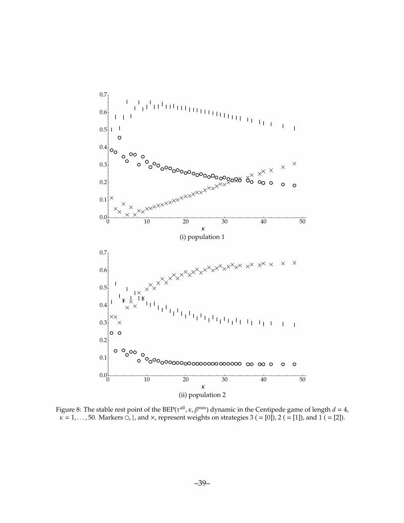
0 10 20 30 40 500.0

0.1

0.2

0.3

0.4

0.5

0.6

0.7

κ

(i) population 1

0 10 20 30 40 500.0

0.1

0.2

0.3

0.4

0.5

0.6

0.7

κ

(ii) population 2

Figure 8: The stable rest point of the BEP(τall, κ, βmin) dynamic in the Centipede game of length d = 4,κ = 1, . . . , 50. Markers �, | , and ×, represent weights on strategies 3 ( = [0]), 2 ( = [1]), and 1 ( = [2]).

–39–

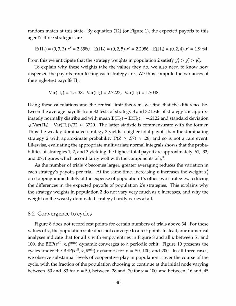
random match at this state. By equation (12) (or Figure 1), the expected payoffs to thisagent’s three strategies are

E(Π1) = (0, 3, 3)·x∗= 2.3580, E(Π2) = (0, 2, 5)·x∗= 2.2086, E(Π3) = (0, 2, 4)·x∗= 1.9964.

From this we anticipate that the strategy weights in population 2 satisfy y∗1 > y∗2 > y∗3 .To explain why these weights take the values they do, we also need to know how

dispersed the payoffs from testing each strategy are. We thus compute the variances ofthe single-test payoffs Π j:

Var(Π1) = 1.5138, Var(Π2) = 2.7223, Var(Π3) = 1.7048.

Using these calculations and the central limit theorem, we find that the difference be-tween the average payoffs from 32 tests of strategy 3 and 32 tests of strategy 2 is approx-imately normally distributed with mean E(Π3) − E(Π2) = −.2122 and standard deviation√

(Var(Π3) + Var(Π2))/32 ≈ .3720. The latter statistic is commensurate with the former.Thus the weakly dominated strategy 3 yields a higher total payoff than the dominatingstrategy 2 with approximate probability P(Z ≥ .57) ≈ .28, and so is not a rare event.Likewise, evaluating the appropriate multivariate normal integrals shows that the proba-bilities of strategies 1, 2, and 3 yielding the highest total payoff are approximately .61, .32,and .07, figures which accord fairly well with the components of y∗.

As the number of trials κ becomes larger, greater averaging reduces the variation ineach strategy’s payoffs per trial. At the same time, increasing κ increases the weight x∗1on stopping immediately at the expense of population 1’s other two strategies, reducingthe differences in the expected payoffs of population 2’s strategies. This explains whythe strategy weights in population 2 do not vary very much as κ increases, and why theweight on the weakly dominated strategy hardly varies at all.

8.2 Convergence to cycles

Figure 8 does not record rest points for certain numbers of trials above 34. For thesevalues of κ, the population state does not converge to a rest point. Instead, our numericalanalyses indicate that for all κ with empty entries in Figure 8 and all κ between 51 and100, the BEP(τall, κ, βmin) dynamic converges to a periodic orbit. Figure 10 presents thecycles under the BEP(τall, κ, βmin) dynamics for κ = 50, 100, and 200. In all three cases,we observe substantial levels of cooperative play in population 1 over the course of thecycle, with the fraction of the population choosing to continue at the initial node varyingbetween .50 and .83 for κ = 50, between .28 and .70 for κ = 100, and between .16 and .45

–40–

x1

x2 x3

y1

y2 y3

Figure 9: The stable rest point in Centipede of length d = 4 under BEP(τall, κ, βmin) dynamics forκ = 1, . . . , 34 trials of each tested strategy. Lighter shading corresponds to larger numbers of trials. Dashed

lines represent boundaries of best response regions.

for κ = 200. These examples illustrate that cooperative behavior can persist even whenagents have substantial amounts of information about opponents’ play.

From a methodological point of view, the existence of almost globally attracting limitcycles under BEP dynamics suggests that solution concepts like S(k) equilibrium andlogit equilibrium that are motivated as steady states of dynamic disequilibrium processesshould be applied with some caution. Existence results for such solution concepts cangenerally be proved by appeals to suitable fixed point theorems. But the fact that staticsolutions exist need not imply that any are stable, and it may happen that no static solutionprovides a good prediction of the behavior of the underlying dynamic process.

9. Discussion

In this paper, we have introduced a class of game dynamics built on natural assump-tions about the information agents obtain when revising, and have shown that thesedynamics lead to cooperative behavior in the Centipede game. One key feature of theagents’ revision process is that conditional on the current population state, the experi-enced payoffs to each strategy are independent of one another. This allows cooperativestrategies with suboptimal expected payoffs to be played with nonnegligible probabilities,even when the testing of each strategy involves substantial numbers of trials. The use ofany such strategy increases the expected payoffs of other cooperative strategies, creatinga virtuous circle that sustains cooperative play.

–41–

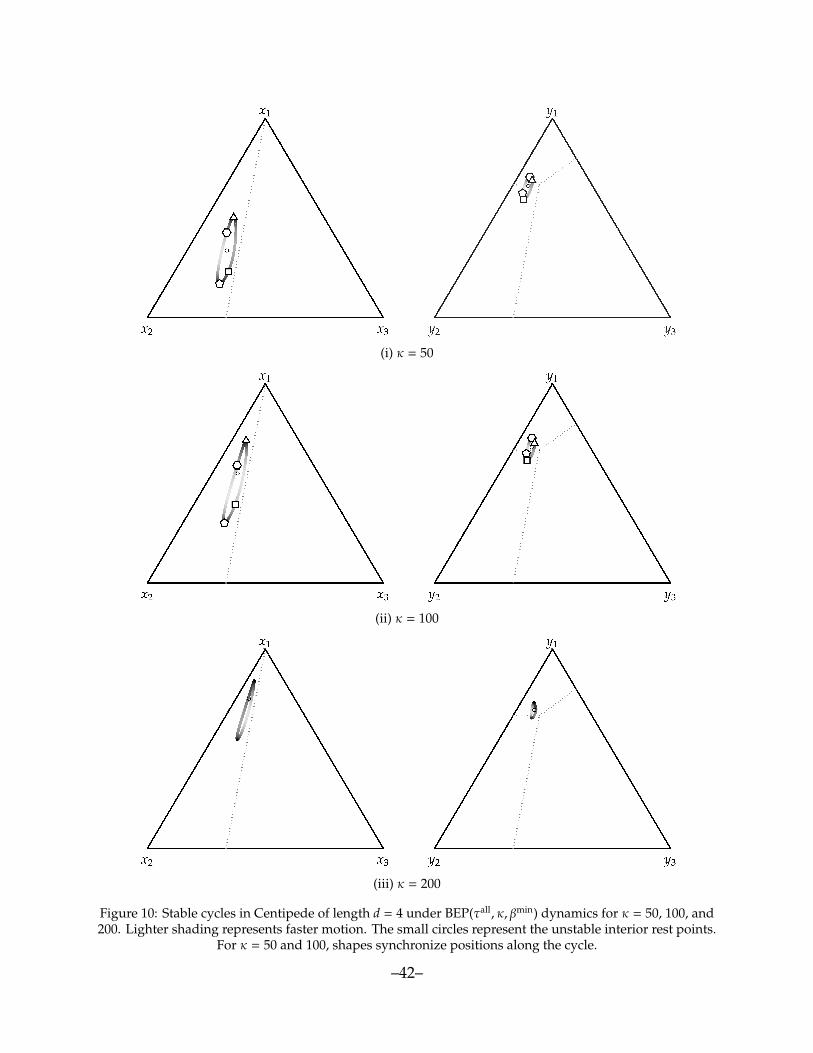
(i) κ = 50

(ii) κ = 100

(iii) κ = 200

Figure 10: Stable cycles in Centipede of length d = 4 under BEP(τall, κ, βmin) dynamics for κ = 50, 100, and200. Lighter shading represents faster motion. The small circles represent the unstable interior rest points.

For κ = 50 and 100, shapes synchronize positions along the cycle.

–42–

9.1 Comparisons to discrete choice models

A related and thoroughly-studied approach to modeling choice under populationgame dynamics is to use constructions from discrete choice theory.41 The most com-mon specification employed is the logit choice model, in large part because of its simplefunctional form.42 Equilibria of the logit model are commonly used in the analysis ofexperimental data, as they offer a convenient way of incorporating suboptimal choicesinto equilibrium predictions.43

Logit dynamics and BEP dynamics share a key feature: both incorporate independentrealizations of the payoffs to different strategies. These dynamics also differ in basicways. While specifying a high noise level for the logit dynamic leads to near-uniformrandomization, choosing small numbers of trials under BEP dynamics yields interestingpredictions of play. In addition, while the payoff perturbations used to define logitdynamics take the same form regardless of the current population state, the variations inpayoffs under BEP dynamics depend on the state in a fundamental way. This allows strictequilibria to be rest points of all BEP dynamics (cf. Observation 2.1), while under logitdynamics the boundary of the state space is always repelling.

From a computational standpoint, logit choice probabilities can be expressed in aclosed form, but one involving transcendental functions. This makes exact computationof logit equilibrium impossible. The fact that BEP dynamics are described by polynomialequations makes them susceptible to analysis using computational algebra, allowing usto obtain exact expressions for rest points, as well as rigorous proofs of dynamic stability.

As important as these operational differences are the conceptual differences betweendiscrete choice and BEP models for games. The former proceed by augmenting a gamewith a payoff noise structure that is completely distinct from the game itself. By contrast,BEP models do not introduce new sources of payoffs. Rather, they drop standard butstrong assumptions concerning knowledge about opponents’ behavior, assuming thatagents make choices using only the information gained from limited experiences of play.This step in the direction of realism leads to a model whose predictions can differ fromtraditional ones and, at least in the case of Centipede, may better reflect observed behavior.

When the number of trials of each tested strategy is not small, the central limit theo-rem allows us to approximate choice probabilities under BEP dynamics by probit choice

41See, e.g., Fudenberg and Levine (1998) and Hofbauer and Sandholm (2002, 2007).42See the previous references, as well as Blume (1997).43McKelvey and Palfrey (1995) introduce equilibrium notions defined in terms of discrete choice models

under the name quantal response equilibrium, and place emphasis on logit equilibrium. McKelvey and Palfrey(1998) extend this notion to extensive form games, focusing on a definition of equilibrium based on the agentnormal form, and use this concept to fit experimental data from the Centipede game.

–43–

probabilities—that is, by probabilities obtained by perturbing strategies’ payoffs withindependent, normally distributed disturbance terms—but with the variances in thesedisturbances depending upon the current state (see Section 8). This fact suggests anapproach to studying the behavior of BEP dynamics with large numbers of trials, forwhich exact expressions are too cumbersome for use even in numerical analysis. We aredeveloping this approach in our current research.

9.2 Analyses of other game dynamics

Our ability to analyze BEP dynamics using tools from computational algebra dependedonly on the fact that these dynamics are described by polynomial equations with rationalcoefficients. There are many other dynamics that share this property, including otherdynamics based on random sampling and various sorts of imitative dynamics.44 Thepowerful algebraic tools used here have the potential to generate new qualitative insightseven about well-studied game dynamics, offering a fertile domain for future work.

9.3 Analyses of general extensive form games

A basic message of our analysis is that natural weakenings of assumptions aboutagents’ knowledge, ones that do not in turn require common knowledge of a more com-plicated interaction, can lead to predictions of play that differ markedly from ones basedon backward induction and that accord in broad terms with experimental and anecdotalevidence. Our analysis has focused on the Centipede game because it provides the sim-plest model of ongoing relationships with a fixed terminal date. It is important to confirmthat the ideas underlying the stability of cooperative behavior here remain relevant inother games in which violations of backward induction can be mutually beneficial, andto identify other properties of games that work for or against cooperative play. We leavethese questions for future research.

44For the former, see Oyama et al. (2015); for the latter, see Taylor and Jonker (1978), Weibull (1995),Hofbauer (1995a), and Sandholm (2010b).

–44–

Appendix

A. Repulsion from the backward induction state

Letting s = s1 + s2, we denote the tangent space of the state space Ξ = X × Y byTΞ = TX × TY = {(z1, z2)′ ∈ Rs :

∑i∈S1 z1

i = 0 and∑

j∈S2 z2j = 0}, and we denote the affine

hull of Ξ by aff(Ξ) = TΞ + ξ†. Writing our dynamics as

(D) ξ = V(ξ),

we have V : aff(Ξ) → TΞ, and so DV(ξ)z ∈ TΞ for all ξ ∈ Ξ and z ∈ TΞ. We can thusview DV(ξ) as a linear map from TΞ to itself, and the behavior of the dynamics in theneighborhood of a rest point is determined by the eigenvalues and eigenvectors of thislinear map. The latter are obtained by computing the eigenvalues and eigenvectors of theproduct matrixΦDV (ξ)Φ, where V : Rs

→ Rs is the natural extension of V to Rs, andΦis the orthogonal projection of Rs onto TΞ, i.e., the block diagonal matrix with diagonalblocks I − 1

s1 11′ ∈ Rs1×s1 and I − 1

s2 11′ ∈ Rs2×s2 , where 1 = (1, . . . , 1)′. Since V maps Ξ into

TΞ, the projection is only needed when there are eigenspaces of DV(ξ) that intersect boththe set TΞ and its complement.

In what follows we write δi∈ Rs and ε j

∈ Rs for the standard basis vectors corre-sponding to strategies i ∈ S1 and j ∈ S2, respectively. We also write all expressions interms of the numbers of decision nodes rather than the numbers of strategies, as doingso usually generates more compact expressions. To eliminate superscripts we use thenotations m ≡ d1 = s1

− 1 and n ≡ d2 = s2− 1 for the numbers of decision nodes.

For BEP dynamics with tie-breaking rule βmin, we prove that the backward inductionstate ξ† is a repellor using the following argument. Computing the eigenvalues andeigenvectors of DV(ξ†) as described above, we find that under each of the three test-setrules we consider, ξ† is a hyperbolic rest point, meaning that all of the eigenvalues havenonzero real part.

The linearization of the dynamic (D) at rest point ξ† is the linear differential equation

(L) z = DV(ξ†)z

on TΞ. The stable subspace Es⊆ TΞ of (L) is the span of the real and imaginary parts of

the eigenvectors and generalized eigenvectors of DV(ξ†) corresponding to eigenvalueswith negative real part. The unstable subspace Eu

⊆ TΞ of (L) is defined analogously. Thebasic theory of linear differential equations implies that solutions to (L) on Es converge to

–45–

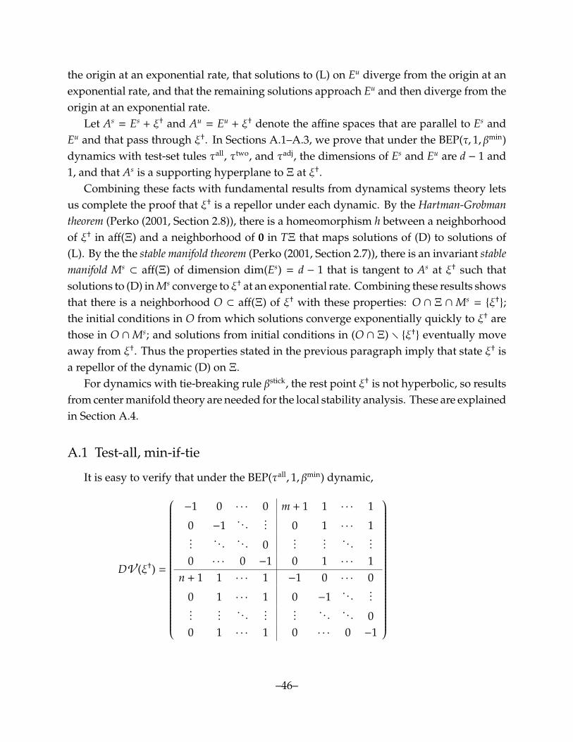
the origin at an exponential rate, that solutions to (L) on Eu diverge from the origin at anexponential rate, and that the remaining solutions approach Eu and then diverge from theorigin at an exponential rate.

Let As = Es + ξ† and Au = Eu + ξ† denote the affine spaces that are parallel to Es andEu and that pass through ξ†. In Sections A.1–A.3, we prove that under the BEP(τ, 1, βmin)dynamics with test-set tules τall, τtwo, and τadj, the dimensions of Es and Eu are d − 1 and1, and that As is a supporting hyperplane to Ξ at ξ†.

Combining these facts with fundamental results from dynamical systems theory letsus complete the proof that ξ† is a repellor under each dynamic. By the Hartman-Grobmantheorem (Perko (2001, Section 2.8)), there is a homeomorphism h between a neighborhoodof ξ† in aff(Ξ) and a neighborhood of 0 in TΞ that maps solutions of (D) to solutions of(L). By the the stable manifold theorem (Perko (2001, Section 2.7)), there is an invariant stablemanifold Ms

⊂ aff(Ξ) of dimension dim(Es) = d − 1 that is tangent to As at ξ† such thatsolutions to (D) in Ms converge to ξ† at an exponential rate. Combining these results showsthat there is a neighborhood O ⊂ aff(Ξ) of ξ† with these properties: O ∩ Ξ ∩Ms = {ξ†};the initial conditions in O from which solutions converge exponentially quickly to ξ† arethose in O ∩Ms; and solutions from initial conditions in (O ∩ Ξ) r {ξ†} eventually moveaway from ξ†. Thus the properties stated in the previous paragraph imply that state ξ† isa repellor of the dynamic (D) on Ξ.

For dynamics with tie-breaking rule βstick, the rest point ξ† is not hyperbolic, so resultsfrom center manifold theory are needed for the local stability analysis. These are explainedin Section A.4.

A.1 Test-all, min-if-tie

It is easy to verify that under the BEP(τall, 1, βmin) dynamic,

DV (ξ†) =

−1 0 · · · 0 m + 1 1 · · · 1

0 −1 . . .... 0 1 · · · 1

.... . . . . . 0

......

. . ....

0 · · · 0 −1 0 1 · · · 1n + 1 1 · · · 1 −1 0 · · · 0

0 1 · · · 1 0 −1 . . ....

......

. . ....

.... . . . . . 0

0 1 · · · 1 0 · · · 0 −1

–46–

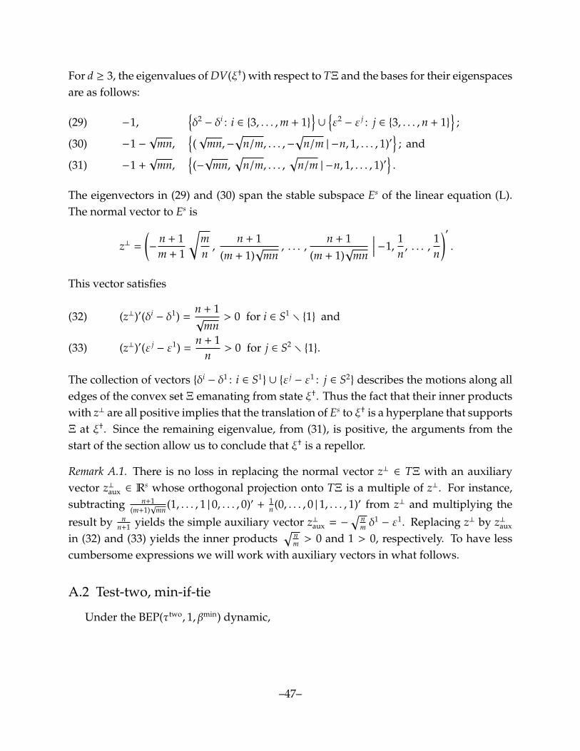
For d ≥ 3, the eigenvalues of DV(ξ†) with respect to TΞ and the bases for their eigenspacesare as follows:

−1,{δ2− δi : i ∈ {3, . . . ,m + 1}

}∪

{ε2− ε j : j ∈ {3, . . . ,n + 1}

};(29)

−1 −√

mn,{(√

mn,−√

n/m, . . . ,−√

n/m | −n, 1, . . . , 1)′}

; and(30)

−1 +√

mn,{(−√

mn,√

n/m, . . . ,√

n/m | −n, 1, . . . , 1)′}.(31)

The eigenvectors in (29) and (30) span the stable subspace Es of the linear equation (L).The normal vector to Es is

z⊥ =

(−

n + 1m + 1

√mn,

n + 1(m + 1)

√mn

, . . . ,n + 1

(m + 1)√

mn

∣∣∣∣ −1,1n, . . . ,

1n

)′.

This vector satisfies

(z⊥)′(δi− δ1) =

n + 1√

mn> 0 for i ∈ S1 r {1} and(32)

(z⊥)′(ε j− ε1) =

n + 1n

> 0 for j ∈ S2 r {1}.(33)

The collection of vectors {δi− δ1 : i ∈ S1

} ∪ {ε j− ε1 : j ∈ S2

} describes the motions along alledges of the convex set Ξ emanating from state ξ†. Thus the fact that their inner productswith z⊥ are all positive implies that the translation of Es to ξ† is a hyperplane that supportsΞ at ξ†. Since the remaining eigenvalue, from (31), is positive, the arguments from thestart of the section allow us to conclude that ξ† is a repellor.

Remark A.1. There is no loss in replacing the normal vector z⊥ ∈ TΞ with an auxiliaryvector z⊥aux ∈ R

s whose orthogonal projection onto TΞ is a multiple of z⊥. For instance,subtracting n+1

(m+1)√

mn (1, . . . , 1 | 0, . . . , 0)′ + 1n (0, . . . , 0 | 1, . . . , 1)′ from z⊥ and multiplying the

result by nn+1 yields the simple auxiliary vector z⊥aux = −

√nm δ

1− ε1. Replacing z⊥ by z⊥aux

in (32) and (33) yields the inner products√

nm > 0 and 1 > 0, respectively. To have less

cumbersome expressions we will work with auxiliary vectors in what follows.

A.2 Test-two, min-if-tie

Under the BEP(τtwo, 1, βmin) dynamic,

–47–

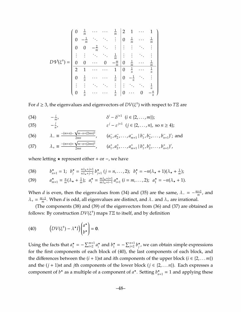
DV (ξ†) =

0 1m · · · · · ·

1m 2 1 · · · 1

0 −1m

. . . . . .... 0 1

m · · ·1m

0 0 −2m

. . ....

......

. . ....

......

. . . . . . 1m

......

. . ....

0 0 · · · 0 −mm 0 1

m · · ·1m

2 1 · · · · · · 1 0 1n · · ·

1n

0 1n · · · · · ·

1n 0 −

1n

. . ....

......

. . . . . ....

.... . . . . . 1

n

0 1n · · · · · ·

1n 0 · · · 0 −

nn

For d ≥ 3, the eigenvalues and eigenvectors of DV(ξ†) with respect to TΞ are

−i

m , δi− δi+1 (i ∈ {2, . . . ,m});(34)

−jn , ε j

− ε j+1 ( j ∈ {2, . . . ,n}, so n ≥ 4);(35)

λ− ≡−(m+n)−

√m−n+(2mn)2

2mn , (a−1 , a−

2 , . . . , a−

m+1 | b−

1 , b−

2 , . . . , b−

n+1)′; and(36)

λ+ ≡−(m+n)+

√m−n+(2mn)2

2mn , (a+1 , a

+2 , . . . , a

+m+1 | b

+1 , b

+2 , . . . , b

+n+1)′,(37)

where letting ? represent either + or −, we have

b?n+1 = 1; b?j =nλ?+ j+1nλ?+ j−1 b?j+1 ( j = n, . . . , 2); b?1 = −n(λ? + 1)(λ? + 1

m );(38)

a?m+1 = nm (λ? + 1

m ); a?i = mλ?+i+1mλ?+i−1 a?i+1 (i = m, . . . , 2); a?1 = −n(λ? + 1).(39)

When d is even, then the eigenvalues from (34) and (35) are the same, λ− = −m+1m , and

λ+ = m−1m . When d is odd, all eigenvalues are distinct, and λ− and λ+ are irrational.

(The components (38) and (39) of the eigenvectors from (36) and (37) are obtained asfollows: By construction DV(ξ†) maps TΞ to itself, and by definition

(40)(DV(ξ†) − λ?I

) a?

b?

= 0.

Using the facts that a?1 = −∑m+1

i=2 a?i and b?1 = −∑n+1

j=2 b?j , we can obtain simple expressionsfor the first components of each block of (40), the last components of each block, andthe differences between the (i + 1)st and ith components of the upper block (i ∈ {2, . . .m})and the ( j + 1)st and jth components of the lower block ( j ∈ {2, . . .n}). Each expresses acomponent of b? as a multiple of a component of a?. Setting b?n+1 = 1 and applying these

–48–

expressions yields (38) and (39), along with the fact that (λ? + 1m )(λ? + 1

n ) = 1.)The eigenvectors in (34)–(36) span the stable subspace Es of the linear equation (L).

The normal vector to Es is the orthogonal projection onto TΞ of the auxiliary vector

z⊥aux = −m−n+√

m−n+(2mn)2

2mn δ1− ε1,

which satisfies

(z⊥)′(δi− δ1) = (z⊥aux)′(δi

− δ1) =m−n+√

m−n+(2mn)2

2mn > 0 for i ∈ S1 r {1}, and

(z⊥)′(ε j− ε1) = (z⊥aux)′(ε j

− ε1) = 1 > 0 for j ∈ S2 r {1}.

Thus the translation of Es to ξ† supports Ξ at ξ†. Since the remaining eigenvalue, from(37), is positive, the arguments from the start of the section imply that ξ† is a repellor.

A.3 Test-adjacent, min-if-tie

Under the BEP(τadj, 1, βmin) dynamic,

DV (ξ†) =

0 12 0 · · · 0 2 1 · · · · · · 1

0 −12

. . . . . .... 0 1 · · · · · · 1

.... . . . . . 1

2 0 0 · · · · · · · · · 0.... . . . . . − 1

2 1.... . . . . . . . .

...

0 · · · · · · 0 −1 0 · · · · · · · · · 02 1 · · · · · · 1 0 1

2 0 · · · 0

0 1 · · · · · · 1 0 −12

. . . . . ....

0 · · · · · · · · · 0.... . . . . . 1

2 0.... . . . . . . . .

....... . . . . . − 1

2 10 · · · · · · · · · 0 0 · · · · · · 0 −1

We first consider the case in which d = 3, for which the eigenvalues and eigenvectors ofDV(x†, y†) with respect to TΞ are:

−1, (0, 2,−2 | − 1, 1)′;(41)

λ− ≡−3−√

174 , (λ− + 1,−λ− − 1, 0 | 1,−1)′; and(42)

λ+ ≡−3+√

174 , (λ+ + 1,−λ+ − 1, 0 | 1,−1)′.(43)

–49–

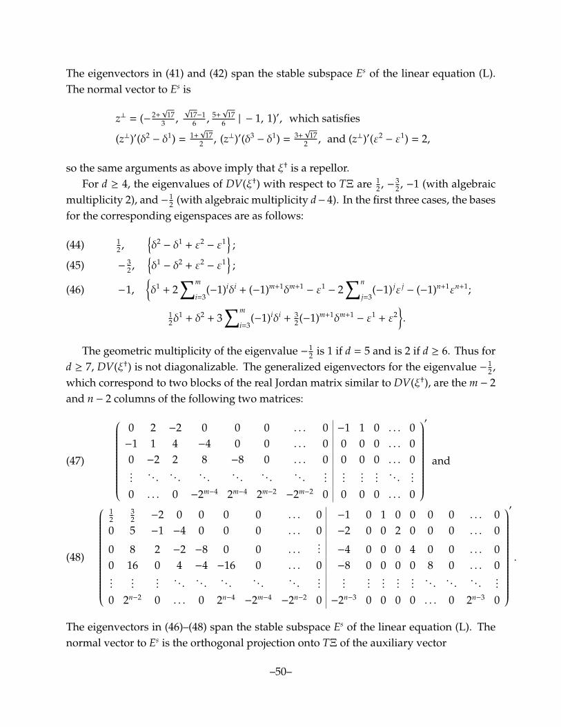
The eigenvectors in (41) and (42) span the stable subspace Es of the linear equation (L).The normal vector to Es is

z⊥ = (− 2+√

173 ,

√17−16 , 5+

√17

6 | − 1, 1)′, which satisfies

(z⊥)′(δ2− δ1) = 1+

√17

2 , (z⊥)′(δ3− δ1) = 3+

√17

2 , and (z⊥)′(ε2− ε1) = 2,

so the same arguments as above imply that ξ† is a repellor.For d ≥ 4, the eigenvalues of DV(ξ†) with respect to TΞ are 1

2 , − 32 , −1 (with algebraic

multiplicity 2), and −12 (with algebraic multiplicity d− 4). In the first three cases, the bases

for the corresponding eigenspaces are as follows:

12 ,

{δ2− δ1 + ε2

− ε1}

;(44)

−32 ,

{δ1− δ2 + ε2

− ε1}

;(45)

−1,{δ1 + 2

∑m

i=3(−1)iδi + (−1)m+1δm+1

− ε1− 2

∑n

j=3(−1) jε j

− (−1)n+1εn+1;(46)

12δ

1 + δ2 + 3∑m

i=3(−1)iδi + 3

2 (−1)m+1δm+1− ε1 + ε2

}.

The geometric multiplicity of the eigenvalue −12 is 1 if d = 5 and is 2 if d ≥ 6. Thus for

d ≥ 7, DV(ξ†) is not diagonalizable. The generalized eigenvectors for the eigenvalue − 12 ,

which correspond to two blocks of the real Jordan matrix similar to DV(ξ†), are the m − 2and n − 2 columns of the following two matrices:

0 2 −2 0 0 0 . . . 0 −1 1 0 . . . 0−1 1 4 −4 0 0 . . . 0 0 0 0 . . . 00 −2 2 8 −8 0 . . . 0 0 0 0 . . . 0...

. . . . . . . . . . . . . . . . . ....

.......... . .

...

0 . . . 0 −2m−4 2m−4 2m−2−2m−2 0 0 0 0 . . . 0

′

and(47)

12

32 −2 0 0 0 0 . . . 0 −1 0 1 0 0 0 0 . . . 0

0 5 −1 −4 0 0 0 . . . 0 −2 0 0 2 0 0 0 . . . 0

0 8 2 −2 −8 0 0 . . .... −4 0 0 0 4 0 0 . . . 0

0 16 0 4 −4 −16 0 . . . 0 −8 0 0 0 0 8 0 . . . 0...

......

. . . . . . . . . . . . . . ....

................ . . . . . . . .

...

0 2n−2 0 . . . 0 2n−4−2m−4

−2n−2 0 −2n−3 0 0 0 0 . . . 0 2n−3 0

′

.(48)

The eigenvectors in (46)–(48) span the stable subspace Es of the linear equation (L). Thenormal vector to Es is the orthogonal projection onto TΞ of the auxiliary vector

–50–

z⊥aux =

m∑i=1

(22−m− 3 · 21−i) δi +

n∑j=1

(22−n− 3 · 21− j) ε j.

Thus z⊥ satisfies

(z⊥)′(δm+1− δ1) = (z⊥aux)′(δm+1

− δ1) = 3 − 22−m > 0,

(z⊥)′(εn+1− ε1) = (z⊥aux)′(εn+1

− ε1) = 3 − 22−n > 0,

(z⊥)′(δi− δ1) = (z⊥aux)′(δi

− δ1) = 3 · (1 − 21−i) > 0 for i ∈ S1 r {1,m + 1}, and

(z⊥)′(ε j− ε1) = (z⊥aux)′(ε j

− ε1) = 3 · (1 − 21− j) > 0 for j ∈ S2 r {1,n + 1}.

Since the remaining eigenvalue, from (44), is positive, the arguments from the start of thesection imply that ξ† is a repellor.

A.4 Test-all, stick/min-if-tie

Under BEP dynamics based on the stick/min-if tie rule βstick, the backward inductionstate ξ† is not a hyperbolic rest point, and in particular has some zero eigenvalues. Toshow that it is nevertheless a repellor, we follow the same line of argument as above,but replace the arguments based on the Hartman-Grobman and stable manifold theoremswith arguments from center manifold theory.

Consider again the dynamic (D) and its linearization at ξ† (L) from the start of thissection. When ξ† is not a hyperbolic rest point of (D), we can define for (L) the stablesubspace Es

⊆ TΞ, the unstable subspace Eu⊆ TΞ, and the center subspace Ec

⊆ TΞ,where the last is the span of the real and imaginary parts of eigenvectors correspondingto eigenvalues with zero real part.

Let Acs = Ec⊕ Es + ξ† be the affine space that is parallel to Ec

⊕ Es and that passesthrough ξ†. Below we show that under the BEP(τall, 1, βstick) dynamic, the subspace Ec

⊕Es

has dimension d − 1, and the affine space Acs is a supporting hyperplane to Ξ at ξ†. Weprove the corresponding results for dynamics based on test-set rules τtwo and τadj in OnlineAppendix V.

Linearization is much less simple for nonhyperbolic rest points than for hyperbolicones—see Perko (2001). However, for our purposes, it is enough that there exists a(local) center-stable manifold Mcs that is tangent to Acs, and is invariant under (D) (Kelley(1967b)). This manifold need not be unique; see Kelley (1967b, Section 4) for an example.45

45Under the BEP(τtwo, 1, βstick) dynamic, the affine set through ξ† defined by the eigenvectors with zeroeigenvalue consists entirely of rest points; see footnote 37 and Online Appendix V.2. This fact and Corollary3.3 of Sijbrand (1985) imply that this affine set is the unique center manifold through ξ†.

–51–

But for any choice of center-stable manifold Mcs, there is a neighborhood O ⊂ aff(Ξ) of ξ†

satisfying O∩Ξ∩Mcs = {ξ†} such that solutions to (D) from initial conditions in (O∩Ξ)r{ξ†}eventually move away from ξ†; see Kelley (1967a, p. 336), or see Perko (2001, Theorem2.12.2) for a closely related and more explicitly presented result. This and the propertiesfrom the previous paragraph imply that ξ† is a repellor of the BEP(τ, 1, βstick) dynamics onΞ.

Turning to the computation, we observe that under the BEP(τall, 1, βstick) dynamic,

DV (ξ†) =

−1 0 · · · 0 m + 1 1 · · · 1

0 −1 . . .... 0 1 · · · 1

.... . . . . . 0

......

. . ....

0 · · · 0 −1 0 1 · · · 1n + 1 1 · · · 1 0 · · · · · · 0

0 1 · · · 1...

. . ....

......

. . ....

.... . .

...

0 1 · · · 1 0 · · · · · · 0

The eigenvalues of DV(ξ†) and bases for their eigenspaces are

0,{ε2− ε j : j ∈ {3, . . . ,n + 1}

};(49)

−1,{δ2− δi : i ∈ {3, . . . ,m + 1}

};(50)

λ− ≡ −12 −

√mn + 1

4 ,{

(−λ−,λ−m, . . . ,

λ−m

∣∣∣∣ −n, 1, . . . , 1)′}

; and(51)

λ+ ≡ −12 +

√mn + 1

4 ,{

(−λ+,λ+

m, . . . ,

λ+

m

∣∣∣∣ −n, 1, . . . , 1)′}.(52)

The eigenvectors in (49) span the center subspace Ec of the linear equation (L), whilethe eigenvectors in (50) and (51) span the stable subspace Es. The normal vector to thehyperplane Ec

⊕ Es is the orthogonal projection onto TΞ of the auxiliary vector

z⊥aux = −

√nmδ1− ε1,

which satisfies

(z⊥)′(δi− δ1) = (z⊥aux)′(δi

− δ1) =√

nm > 0 for i ∈ S1 r {1} and

(z⊥)′(ε j− ε1) = (z⊥aux)′(εi

− ε1) = 1 > 0 for j ∈ S2 r {1}.

–52–

Since the remaining eigenvalue, from (52), is positive, the arguments above imply that ξ†

is a repellor.

B. Local stability analysis of interior rest points

The interior rest pointξ∗ of the dynamic x = V(x) is locally stable if all eigenvalues of thederivative matrix DV(ξ∗) have negative real part. Since each entry of the derivative matrixDV (ξ∗) is a polynomial with many terms that is evaluated at state whose components arealgebraic numbers, it is not feasible to compute its eigenvalues exactly. We circumventthis problem by computing the eigenvalues of the derivative matrix at a nearby rationalstate ξ, and making use of a bound on the distances between the eigenvalues of the twomatrices. This bound is established in Proposition B.1, and a more quickly computablealternative is provided in Proposition III.4 of the online appendix.

As in Appendix A, let s = s1 + s2 = d + 2, let ξ = V(ξ), V : aff(Ξ) → TΞ denote aninstance of the BEP dynamics (B), and let V : Rs

→ Rs denote the natural extension of Vto Rs. Observe that if DV (ξ) is diagonalizable, then so is DV(ξ), and all eigenvalues ofthe latter are eigenvalues of the former. To state the proposition, we write S = S1

∪ S2 andomit population superscripts to define

(53) ∆ = maxi∈S

maxk∈S

∑j∈S

∂2Vi

∂ξ j∂ξk(1, . . . , 1 | 1, . . . , 1).

Proposition B.1. Suppose that DV (ξ) is (complex) diagonalizable with DV (ξ) = Q diag(λ)Q−1,and let λ∗ be an eigenvalue of DV (ξ∗). Then there is an eigenvalue λi of DV (ξ) such that

(54)∣∣∣λ∗ − λi

∣∣∣ < 2∆

ss/2−1

tr(Q∗Q)s/2

|det(Q) |

∑k∈S

|ξk − ξ∗k |.

The eigenvalue perturbation theorem (56) that begins the proof of the propositionbounds the distances between the eigenvalues of DV (ξ∗) and DV (ξ), but neither term onits right-hand side is feasible to compute. The second paragraph of the proof provides abound on the condition number κ∞(Q) that does not require the computation of the inverseof the (algebraic-valued) eigenvector matrix Q. The third paragraph provides a boundon the norm of DV (ξ) −DV (ξ∗), which is needed because numerically evaluating of theentries of DV (ξ∗) with guaranteed precision is computationally infeasible. Two furtherdevices that we employ to improve the bound and speed its computation are describedafter the proof of the proposition.

–53–

Proof. For M ∈ Rs×s, let

(55) |||M|||∞ = max1≤i≤s

s∑j=1

|Mi j|.

denote the maximum row sum norm of M. Let κ∞(Q) = |||Q|||∞ |||Q−1|||∞ be the condition

number of Q with respect to norm (55). The following eigenvalue perturbation theorem(Horn and Johnson (2013, Observation 6.3.1)) follows from the Gersgorin disk theoremand the submultiplicativity of matrix norms:

(56)∣∣∣λ∗ − λi

∣∣∣ ≤ κ∞(Q) |||DV (ξ) −DV (ξ∗)|||∞.

To bound κ∞(Q), let |||M|||2 denote the spectral norm of M (i.e., the largest singularvalue of M), and let κ2(Q) = |||Q|||2 |||Q−1

|||2 be the condition number of Q with respect tothis norm. Since the maximum row sum and spectral norms differ by a factor of at most√

s (Horn and Johnson (2013, Problem 5.6.P23)), it follows that

(57) κ∞(Q) ≤ sκ2(Q).

Also, Guggenheimer et al. (1995) (see also Merikoski et al. (1997)) show that

(58) κ2(Q) <2

|det(Q) |

(tr(Q∗Q)

s

)s/2

.

To bound the final expression in (56), recall that each component of expression (B)for the BEP dynamics x = V (x) is the difference between a sum of monomials in thecomponents of ξwith positive coefficients and a linear term. Thus the second derivativesof Vi(ξ) are sums of monomials with positive coefficients. Since every component of everystate ξ ∈ Ξ is at most 1, we therefore have

(59) maxξ∈Ξ

∣∣∣∣∣∣ ∂2Vi

∂ξ j∂ξk(ξ)

∣∣∣∣∣∣ ≤ ∂2Vi

∂ξ j∂ξk(1, . . . , 1 | 1, . . . , 1).

Thus the fundamental theorem of calculus, (59), and (53) imply that

|||DV (ξ) −DV (ξ∗)|||∞ ≤ maxi∈S

∑j∈S

∑k∈S

∂2Vi

∂ξ j∂ξk(1, . . . , 1 | 1, . . . , 1) × |ξk − ξ

∗k |

≤ ∆∑k∈S

|ξk − ξ∗k |.(60)

–54–

Combining inequalities (56), (57), (58), and (60) yields inequality (54). �

When applying Proposition B.1, one can choose Q to be any matrix of eigenvectorsof DV (ξ). Guggenheimer et al. (1995) suggest that choosing the eigenvectors to haveEuclidean norm 1 (which if done exactly makes the expression in parentheses in (58)equal 1) leads to the lowest bounds. We apply this normalization in the final step ofour analysis. Finally, recalling that s = d + 2, we can speed up calculations substantiallyby replacing the s × s matrix DV (ξ∗) with a d × d matrix with the same eigenvalues asDV(ξ) : TΞ → TΞ. We accomplish this by adapting a dimension-reduction method fromSandholm (2007). See Proposition III.4 in the online appendix for the bound’s final form.

To use this bound to establish the stability of the interior rest point ξ∗, we choose arational point ξ close to ξ∗, compute the eigenvalues of the derivative matrix DV(ξ), andevaluate the bound from Proposition III.4. The eigenvalues of DV(ξ) all have negativereal part so long as ξ is reasonably close to ξ∗.46 If ξ is close enough to ξ∗ that thebound is smaller than the magnitude of the real part of any eigenvalue of DV(ξ), we canconclude that the eigenvalues of DV(ξ∗) all have negative real part, and hence that ξ∗ isasymptotically stable.

Selecting state ξ involves a tradeoff: choosing ξ closer to ξ∗ reduces the bound, butdoing so also leads the components of ξ to have larger numerators and denominators,which slows the computation of the bound significantly. In all cases, we are able to chooseξ satisfactorily and to conclude that ξ∗ is asymptotically stable. For further details abouthow the computations are implemented, see the online appendix.

C. Inward motion from the boundary

The following differential inequality will allow us to obtain simple lower bounds onthe use of initially unused strategies. In all cases in which we apply the lemma, v(0) = 0.

Lemma C.1. Let v : [0,T]→ R+ satisfy v(t) ≥ a(t) − v(t) for some a : [0,T]→ R+. Then

(61) v(t) ≥ e−t

(v(0) +

∫ t

0es a(s) ds

)for all t ∈ [0,T].

Proof. Clearly v(t) = v(0) +∫ t

0v(s) ds ≥ v(0) +

∫ t

0(a(s) − v(s)) ds. The final expression is

the time t value of the solution to the differential equation v(s) + v(s) = a(s) with initial

46Among the cases in which we solve for ξ∗ exactly, the smallest magnitude of a real part of an eigenvalueoccurs under the BEP(τadj, 1, βmin) dynamic when d = 7, in which case there is an eigenvalue approximatelyequal to −.1125. See Online Appendix IX.

–55–

condition v(0). Using the integrating factor es to solve this equation yields the right-handside of (61). �

For the analysis to come, it will be convenient to work with the set S = S1∪ S2 of

all strategies from both populations, and to drop population superscripts from notationrelated to the state—for instance, writing ξi rather than ξp

i .We use Lemma C.1 to prove inward motion from the boundary under BEP dynamics

in the following way. Write ξi = ri(ξ) − ξi, where ri(ξ) is the polynomial appearing inthe formula (B) for the BEP(τ, 1, β) dynamic. Let {ξ(t)}t≥0 be the solution of (B) withinitial condition ξ(0). Let S0 = supp(ξ(0)) and Q = min{ξh(0) : h ∈ S0}, and, finally, letS1 = {i ∈ S r S0 : ri(ξ(0)) > 0} and R = 1

2 min{rk(ξ(0)) : rk(ξ(0)) > 0}.By the continuity of (B), there is a neighborhood O ⊂ Ξ of ξ(0) such that every χ ∈ O

satisfies χh > Q for all h ∈ S0 and χi ≥ R for all i ∈ S1 . And since (B) is smooth, there is atime T > 0 such that ξ(t) ∈ O for all t ∈ [0,T]. Thus applying Lemma C.1 shows that

(62) ξi(t) ≥ R(1 − e−t) for all t ∈ [0,T] and i ∈ S1.

Now let S2 be the set of j < S0 ∪ S1 for which there is a term of polynomial r j whosefactors all correspond to elements of S0 or S1. If this term has a factors in S0, b factors inS1, and coefficient c, then the foregoing claims and Lemma C.1 imply that

(63) ξ j(t) ≥ c Qa e−t∫ t

0es(R(1 − e−s))b ds for all t ∈ [0,T].

Proceeding sequentially, we can obtain positive lower bounds on the use of any strategyfor times t ∈ (0,T] by considering as-yet-unconsidered strategies k whose polynomials rk

have a term whose factors all correspond to strategies for which lower bounds havealready been obtained. Below, we prove that solutions to the BEP(τall, 1, βmin) dynamicfrom states ξ(0) , ξ† immediately enter int(Ξ) by showing that the strategies in S r S0 canbe considered in a sequence that satisfies the property just stated. The proofs for otherBEP dynamics are described in the remarks that follow.

To proceed, we use the notations i[1] and i[2] to denote the ith strategies of players 1 and2. We also introduce the linear order ≺ on S defined by 1[1]

≺ 1[2]≺ 2[1]

≺ 2[2]≺ 3[1]

≺ . . . ,which arranges the strategies according to how early they stop play in Centipede.

Proof of Proposition 5.5. Fix an initial condition ξ(0) , ξ†. We can sequentially add allstrategies in S r S0 in accordance with the property above as follows:

(I) First, we add the strategies {i ∈ S rS0 : i ≺ max S0} in decreasing order. At the pointthat i has been added, i’s successor h has already been added, and strategy i is the unique

–56–

best response when the revising agent tests all strategies against opponents playing h. LetS I denote the set of strategies added during this stage. The assumption that ξ(0) , ξ†

implies that S0 ∪ S I contains 1[1], 1[2], and 2[1].(II) Second, we add the strategies j ∈ S2r(S0∪S I). We can do so because j is the unique

best response when it is tested against 2[1] and all other strategies are tested against 1[1].(III) Third, we add the strategies k ∈ S1r (S0∪S I). We can do so because k is the unique

best response when it is tested against 2[2] and other strategies are tested against 1[2]. �

Remark C.2. (i) Since the preceding argument only used unique best responses, it appliesequally well under any tie-breaking rule. In the case of the uniform-if-tie rule βunif, asimple argument along the lines above also establishes motion into the interior from thebackward induction state ξ†.

(ii) Likewise, while Proposition 5.5 concerns the test-all rule τall, the analysis aboveworks equally well for the test-two rule τtwo.

(iii) To establish entry into int(Ξ) under the test-adjacent rule τadj, we must start withthe following preliminary stage: Let m = max S0 be a population p strategy, let q , p,and let ` = max S0 ∩ Sq. In the preliminary stage, we sequentially add strategies in theset {i ∈ Sp r S0 : i ≺ m} in decreasing order, stopping once we add the successor of `. Wecan add each such strategy h because player p’s succeeding strategy is either in S0 or hasalready been added, so that agents playing that strategy can have strategy h in their testset; and because the revising agent will prefer h to the succeeding strategy if both aretested against opponents playing ` ≺ h. After these strategies are added, stage (I) canproceed, but replacing max S0 with `, and stages (II) and (III) work as before providedthat the strategies added in these stages are added in increasing order.

References

Akritas, A. G. (2010). Vincent’s theorem of 1836: Overview and future research. Journal ofMathematical Sciences, 168:309–325.

Becker, E., Marinari, M. G., Mora, T., and Traverso, C. (1994). The shape of the ShapeLemma. In von zur Gathen, J. and Giesbrecht, M., editors, ISSAC ’94: Proceedings of theinternational symposium on symbolic and algebraic computation, pages 129–133. ACM.

Ben-Porath, E. (1997). Rationality, Nash equilibrium and backwards induction in perfect-information games. Review of Economic Studies, 64:23–46.

–57–

Benaım, M. and Weibull, J. W. (2003). Deterministic approximation of stochastic evolutionin games. Econometrica, 71:873–903.

Binmore, K. (1987). Modeling rational players. Economics and Philosophy, 3-4:179–214 and9–55.

Binmore, K. (1998). Game Theory and the Social Contract, Volume 2: Just Playing. MIT Press,Cambridge.

Bjornerstedt, J. and Weibull, J. W. (1996). Nash equilibrium and evolution by imitation. InArrow, K. J. et al., editors, The Rational Foundations of Economic Behavior, pages 155–181.St. Martin’s Press, New York.

Blume, L. E. (1997). Population games. In Arthur, W. B., Durlauf, S. N., and Lane, D. A.,editors, The Economy as an Evolving Complex System II, pages 425–460. Addison-Wesley,Reading, MA.

Brandenburger, A., Friedenberg, A., and Keisler, H. J. (2008). Admissibility in games.Econometrica, 76:307–352.

Buchberger, B. (1965). Ein Algorithmus zum Auffinden der Basiselemente des Restklassenringsnach einem nulldimensionalen Polynomideal. PhD thesis, University of Innsbruck. Trans-lated by M.P. Abramson as “An algorithm for finding the basis elements of the residueclass ring of a zero-dimensional polynomial ideal” in Journal of Symbolic Computation 41(2006), 475–511.

Cardenas, J. C., Mantilla, C., and Sethi, R. (2015). Stable sampling equilibrium in commonpool resource games. Games, 6:299–317.

Cohen, H. (1993). A Course in Computational Algebraic Number Theory. Springer, Berlin.

Collins, G. E. (1975). Quantifier elimination for the theory of real closed fields by cylin-drical algebraic decomposition. In Second GI Conference on Automata Theory and FormalLanguages, volume 33 of Lecture Notes in Computer Science, pages 134–183. Springer,Berlin.

Cox, D., Little, J., and O’Shea, D. (2015). Ideals, Varieties, and Algorithms: An Introductionto Computational Algebraic Geometry and Commutative Algebra. Springer International,Cham, Switzerland, fourth edition.

Cressman, R. (1996). Evolutionary stability in the finitely repeated prisoner’s dilemmagame. Journal of Economic Theory, 68:234–248.

Cressman, R. (2003). Evolutionary Dynamics and Extensive Form Games. MIT Press, Cam-bridge.

Cressman, R. and Schlag, K. H. (1998). On the dynamic (in)stability of backwards induc-tion. Journal of Economic Theory, 83:260–285.

–58–

Dekel, E. and Gul, F. (1997). Rationality and knowledge in game theory. In Kreps, D. M.and Wallis, K. F., editors, Advances in Economics and Econometrics: Theory and Applications,volume 1, pages 87–172. Cambridge University Press, Cambridge.

Droste, E., Kosfeld, M., and Voorneveld, M. (2003). Best-reply matching in games. Mathe-matical Social Sciences, 46:291–309.

Dummit, D. S. and Foote, R. M. (2004). Abstract Algebra. Wiley, Hoboken, NJ, third edition.

Fudenberg, D. and Levine, D. K. (1998). The Theory of Learning in Games. MIT Press,Cambridge.

Gilboa, I. and Matsui, A. (1991). Social stability and equilibrium. Econometrica, 59:859–867.

Guggenheimer, H. W., Edelman, A. S., and Johnson, C. R. (1995). A simple estimate of thecondition number of a linear system. College Mathematics Journal, 26:2–5.

Halpern, J. Y. (2001). Substantive rationality and backward induction. Games and EconomicBehavior, 37:425–435.

Hofbauer, J. (1995a). Imitation dynamics for games. Unpublished manuscript, Universityof Vienna.

Hofbauer, J. (1995b). Stability for the best response dynamics. Unpublished manuscript,University of Vienna.

Hofbauer, J. and Sandholm, W. H. (2002). On the global convergence of stochastic fictitiousplay. Econometrica, 70:2265–2294.

Hofbauer, J. and Sandholm, W. H. (2007). Evolution in games with randomly disturbedpayoffs. Journal of Economic Theory, 132:47–69.

Hofbauer, J. and Sandholm, W. H. (2011). Survival of dominated strategies under evolu-tionary dynamics. Theoretical Economics, 6:341–377.

Horn, R. A. and Johnson, C. R. (2013). Matrix Analysis. Cambridge University Press, NewYork, second edition.

Jehiel, P. (2005). Analogy-based expectation equilibrium. Journal of Economic Theory,123:81–104.

Kelley, A. (1967a). Stability of the center-stable manifold. Journal of Mathematical Analysisand Applications, 18:336–344.

Kelley, A. (1967b). The stable, center-stable, center, center-unstable, and unstable mani-folds. Journal of Differential Equations, 3:546–570.

Kosfeld, M., Droste, E., and Voorneveld, M. (2002). A myopic adjustment process leadingto best reply matching. Journal of Economic Theory, 40:270–298.

–59–

Kreindler, G. E. and Young, H. P. (2013). Fast convergence in evolutionary equilibriumselection. Games and Economic Behavior, 80:39–67.

Kreps, D. M., Milgrom, P., Roberts, J., and Wilson, R. (1982). Rational cooperation in thefinitely repeated Prisoner’s Dilemma. Journal of Economic Theory, 27:245–252.

Kubler, F., Renner, P., and Schmedders, K. (2014). Computing all solutions to polyno-mial equations in economics. In Schmedders, K. and Judd, K. L., editors, Handbook ofComputational Economics, volume 3, pages 599–652. Elsevier, Amsterdam.

Mantilla, C., Sethi, R., and Cardenas, J. C. (2017). Efficiency and stability of samplingequilibrium in public good games. Unpublished manuscript, Universidad del Rosario,Columbia University, and Universidad de Los Andes.

McKelvey, R. D. and Palfrey, T. R. (1992). An experimental study of the centipede game.Econometrica, 60:803–836.

McKelvey, R. D. and Palfrey, T. R. (1995). Quantal response equilibria for normal formgames. Games and Economic Behavior, 10:6–38.

McKelvey, R. D. and Palfrey, T. R. (1998). Quantal response equilibria for extensive formgames. Experimental Economics, 1:9–41.

McNamee, J. M. (2007). Numerical Methods for Roots of Polynomials, Part I. Elsevier, Ams-terdam.

Merikoski, J. K., Urpala, U., Virtanen, A., Tam, T.-Y., and Uhlig, F. (1997). A best upperbound for the 2-norm condition number of a matrix. Linear Algebra and its Applications,254:355–365.

Osborne, M. J. and Rubinstein, A. (1998). Games with procedurally rational players.American Economic Review, 88:834–847.

Oyama, D., Sandholm, W. H., and Tercieux, O. (2015). Sampling best response dynamicsand deterministic equilibrium selection. Theoretical Economics, 10:243–281.

Perea, A. (2014). Belief in the opponents’ future rationality. Games and Economic Behavior,83:231–254.

Perko, L. (2001). Differential Equations and Dynamical Systems. Springer, New York, thirdedition.

Ponti, G. (2000). Cycles of learning in the Centipede game. Games and Economic Behavior,30:115–141.

Radner, R. (1980). Collusive behavior in noncooperative epsilon-equilibria of oligopolieswith long but finite lives. Journal of Economic Theory, 22:136–154.

–60–

Reny, P. J. (1992). Backward induction, normal form perfection, and explicable equilibria.Econometrica, 60:627–649.

Robson, A. and Vega-Redondo, F. (1996). Efficient equilibrium selection in evolutionarygames with random matching. Journal of Economic Theory, 70:65–92.

Rosenthal, R. W. (1981). Games of perfect information, predatory pricing and the chain-store paradox. Journal of Economic Theory, 25:92–100.

Samuelson, L. (1992). Dominated strategies and common knowledge. Games and EconomicBehavior, 4:284–313.

Sandholm, W. H. (2001). Almost global convergence to p-dominant equilibrium. Interna-tional Journal of Game Theory, 30:107–116.

Sandholm, W. H. (2003). Evolution and equilibrium under inexact information. Gamesand Economic Behavior, 44:343–378.

Sandholm, W. H. (2007). Evolution in Bayesian games II: Stability of purified equilibria.Journal of Economic Theory, 136:641–667.

Sandholm, W. H. (2010a). Pairwise comparison dynamics and evolutionary foundationsfor Nash equilibrium. Games, 1:3–17.

Sandholm, W. H. (2010b). Population Games and Evolutionary Dynamics. MIT Press, Cam-bridge.

Sandholm, W. H. (2015). Population games and deterministic evolutionary dynamics. InYoung, H. P. and Zamir, S., editors, Handbook of Game Theory, volume 4, pages 703–778.Elsevier, Amsterdam.

Sethi, R. (2000). Stability of equilibria in games with procedurally rational players. Gamesand Economic Behavior, 32:85–104.

Sijbrand, J. (1985). Properties of center manifolds. Transactions of the American MathematicalSociety, 289:431–469.

Stalnaker, R. (1996). Knowledge, belief, and counterfactual reasoning in games. Economicsand Philosophy, 12:133–163.

Taylor, P. D. and Jonker, L. (1978). Evolutionarily stable strategies and game dynamics.Mathematical Biosciences, 40:145–156.

von zur Gathen, J. and Gerhard, J. (2013). Modern Computer Algebra. Cambridge UniversityPress, Cambridge, third edition.

Weibull, J. W. (1995). Evolutionary Game Theory. MIT Press, Cambridge.

–61–

Xu, Z. (2016). Convergence of best-response dynamics in extensive-form games. Journalof Economic Theory, 162:21–54.

Young, H. P. (1993). The evolution of conventions. Econometrica, 61:57–84.

Young, H. P. (1998). Individual Strategy and Social Structure. Princeton University Press,Princeton.

–62–