CBP/TRS-282-06

Best Management Practices for Sediment Control and Water Clarity Enhancement

October 2006

ACKNOWLEDGEMENTS This document was a collaborative effort of the Sediment Workgroup of the Chesapeake Bay Program’s Nutrient Subcommittee, the presenters of best management practice information from the Chesapeake Bay Program’s Sediment BMP Workshop of February 2003, and many others. Many thanks to everyone who contributed their time and expertise, and particularly to the following people for their significant contributions: Lee Hill, Virginia Department of Conservation and Recreation Cameron Wiegand, Department of Environmental Protection-Watershed Management Division, Montgomery County, Maryland Meosotis Curtis, Department of Environmental Protection-Watershed Management Division, Montgomery County, Maryland Ted Graham, Metropolitan Washington Council of Governments Kelly Shenk, US EPA, Chesapeake Bay Program Office Roger I. E. Newell, Horn Point Laboratory, University of Maryland Center for Environmental Science Mike Naylor, Maryland Department of Natural Resources Becky Thur, Chesapeake Research Consortium Peter Bergstrom, National Oceanic and Atmospheric Administration, Chesapeake Bay Program Office Sean Smith, Landscape and Watershed Analysis, Maryland Department of Natural Resources Judy Okay, US Forest Service, Chesapeake Bay Program Office Keely Clifford, US EPA, Chesapeake Bay Program Office Mike Langland, US Geological Survey Reggie Parrish. US EPA, Chesapeake Bay Program Office Tom Simpson, University of Maryland Jeff Sweeney, University of Maryland, Chesapeake Bay Program Office Adam Zimmerman, Chesapeake Research Consortium, Chesapeake Bay Program Office

Cover photo: An area of reconstructed shoreline and marsh habitat. Mike Land, Chesapeake Bay Program.

2

TABLE OF CONTENTS Preface 3 Introduction The Sediment Story 4 Chesapeake Bay Program Commitment 5 Best Management Practice Summaries Riparian Buffers 7 Stream Restoration 13 Urban Stormwater Management 24 Structural Shoreline Erosion Controls 36 Effects of Submerged Aquatic Vegetation (SAV) Upon Estuarine Sediment Processes 42 Oyster Reef Restoration and Oyster Aquaculture 52 Appendix: Meeting Summary Sediment BMP Workshop Agenda 60 Meeting Minutes 61 Presenters 64 Attendees 64 Figures 1. Diagram of riparian buffer with recommended width for specific objectives 7 2. 2004 riparian forest buffer implementation levels, by jurisdiction 11 3. 2004 agricultural riparian grass buffer implementation levels, by jurisdiction 11 4. Picture: Northwest Branch Stream, Montgomery County, before restoration 14 5. Picture: Northwest Branch Stream, Montgomery County, after restoration 14 6. Stream restoration practices associated with design objectives 16 7. Stream restoration reduction efficiencies 18 8. 2004 stream restoration implementation levels, by jurisdiction 19 9. Urban stormwater BMP categories and BMP definitions 24 10. Pollutant removal efficiencies for urban stormwater BMP categories 30 11. 2004 urban stormwater management implementation levels, by jurisdiction 33 12. Picture: Stone revetment on the Potomac River, Virginia 36 13. Picture: Offshore breakwater 37 14. Picture: Headland control system using widely spaced breakwaters 37 15. Diagram of a typical cross-section of a breakwater system 38 16. Picture: The water-clarifying effect of SAV beds on suspended sediment 42 17. Characteristics of SAV communities relevant to estuarine sediment processes 45

3

PREFACE The Chesapeake Bay Program (CBP) hosted a workshop in Annapolis, Maryland

on February 24-25, 2003, at which sediment experts shared information related to sediment best management practices (BMPs). The information presented on selected BMPs has been summarized in this document, and is intended to assist the CBP’s Sediment Workgroup (SedWG) as it moves to the next generation of sediment controls and other practices to improve water clarity in riverine, tidal and near shore areas. In order to provide a thorough summary of each BMP to the workgroup, experts from within the CBP community have contributed to the presenters’ information. Each final BMP summary has received the approval of the expert who presented the information at the workshop.

Sediment controls, clarity enhancement practices and our understanding of sediment processes have advanced since the workshop. For instance, although workshop discussion placed some emphasis on emerging nonstructural/living shoreline approaches, these have become the dominant approach to shore erosion control. The recent concept of “shoreline ecosystem restoration” (i.e., the management of reaches to improve clarity while providing natural shoreline functions, such as beaches and natural cliffs) is challenging traditional, parcel-based shoreline erosion control that usually did not account for adjacent impacts.

Regardless of the progress of sediment science and the application of sediment BMPs, this document remains relevant as a launching point for the SedWG’s efforts to achieve water clarity standards through reducing sediment inputs and managing shorelines and near shore areas. The SedWG recently committed to developing and delineating sedimentsheds, which are the areas or sources of sediment that influence clarity in a submerged aquatic vegetation (SAV) shallow water designated use area. These shallow-water SAV habitats now have state water clarity standards. The workgroup has also set an ambitious goal of developing a sediment budget for each sediment shed.

4

INTRODUCTION

The Sediment Story Sediment is generated by natural weathering of rocks and soils, accelerated erosion of lands, streams and shorelines caused by agricultural and urban development, and resuspension of previously eroded sediments that are stored in stream corridors and in the Chesapeake Bay. Sediment is composed of loose particles of clay, silt and sand. Major sediment sources in the Chesapeake Bay watershed include upland or watershed surfaces and stream corridors. Along the Bay’s shoreline, the primary sources of sediment are from tidal erosion (shoreline erosion, near-shore erosion and near-shore resuspension), ocean input, and biological production. It is estimated that watershed sources contribute approximately 61 percent of the sediment load to the Bay, tidal erosion 26 percent and oceanic input the remaining 13 percent. It is estimated that approximately 8.5 million metric tons of sediment enters the Bay each year. Excess suspended sediment is one of the most important contributors to degraded water quality and has adverse effects on critical habitats and living resources in the Chesapeake Bay and its watershed. Sediment suspended in the water column can reduce water clarity and increase light attenuation such that light penetration is below that needed to support healthy submerged aquatic vegetation (SAV). SAV beds are an important biological resource in estuaries, providing critical habitat and influencing the physical, chemical, and biological conditions of the estuary. In addition to its effect on water clarity, excess sediment can have other adverse effects on ecosystems. For example, sediment can carry toxic contaminants, pathogens and phosphorous (P) that negatively affect fisheries and other living resources. Excessive sedimentation also can degrade the vitality of oyster beds and other benthic (bottom-dwelling) organisms in the Bay and affect commercial shipping and recreational boating by accumulating in shipping channels. In the Bay watershed, sediment is listed as the primary cause of impairment in many streams where it can severely degrade stream habitat and decrease benthic populations. From the standpoint of water clarity, one of the most important characteristics of Bay sediment involves the distinction between fine-grained sediment, which refers to the clay and silt-sized fractions, and coarse-grained sediment, which refers to the sand and pebble- sized fractions. This fine/coarse distinction is important because most coarse material is transported along the bottom of rivers and the Bay and has little effect on light penetration. In contrast, fine-grained sediment commonly is in suspension and, depending on its abundance, grain-size distribution, and degree of aggregation, can play an important role in the degradation of water clarity in the Bay. Erosion from upland land surfaces and erosion of stream corridors (banks and channels) are the two most important sources of sediment coming from the watershed. Sediment

5

erosion is a natural process influenced by geology, soil characteristics, land cover and use, topography, and climate. Some generalizations can be made about erosion, sediment yield (mass per unit area per unit time), and land use in the Bay watershed: • For the entire Chesapeake Bay region, river basins with the highest percentage of

agricultural land use have the highest annual sediment yields, and basins with the highest percentage of forest cover have the lowest annual sediment yields.

• Lands under construction can contribute the most sediment of all land uses. After development is completed, erosion rates are lower; however, sediment yield from urbanized areas can remain high because of increased stream corridor erosion due to altered hydrology.

• Most watershed sediment is transported when streams reach bankfull conditions, which take place on average every 1-2 years during large storm events.

The contribution of tidal erosion to total suspended sediment deserves special comment for several reasons. First, shorelines are receding because of the relatively rapid rate of sea-level rise (1.3 ft for the last century) in the Chesapeake Bay and Mid-Atlantic coast. This rate is twice that of the worldwide average and is the result of regional land subsidence and ocean warming that causes sea level rise. A second critical aspect of tidal erosion is that the relative contribution of tidal erosion is variable, and may be as high as 80 percent or more of the total fine-grained sediment load in the central part of the main stem, south of the Estuarine Turbidity Maximum zone (where fresh river water meets salt water from the Bay), and in the central regions of large tidal tributaries. The third important aspect of tidal erosion involves potential management efforts to reduce total sediment input into the Bay system. Sediment derived from uplands and stream channels can take years to decades to actually reach the lower tidal tributaries and the main stem of the Bay. Although transit times are not known precisely, it is clear that the implementation of management practices in the watershed most likely will not have an immediate effect on Bay water clarity. In contrast, management actions to protect and maintain the extensive shorelines and near-shore areas of the Bay system may have a more immediate effect on decreasing suspended sediment and increasing water clarity in the near-shore SAV-designated growth areas. For more information, please read Sediment in the Chesapeake Bay and Management Issues: Tidal Erosion Processes, available online at http://www.chesapeakebay.net/pubs/doc-tidalerosionChesBay.pdf. Chesapeake Bay Program Commitment In the Chesapeake 2000 agreement, Bay partners committed to correct sediment-related problems in the Bay and its tributaries as part of efforts to remove the Bay from the list of impaired waters by the year 2010. In 2003, the Chesapeake Bay Program partners agreed to reduce upland sediment pollution to help achieve the water clarity in tidal shallow water habitats necessary to restore 185,000 acres of SAV. These goals, adopted as loading caps allocated by major tributary basins by jurisdiction, were based on load-

6

based sediment reductions estimated from management actions directed toward reducing P runoff. To meet this goal, the federal, state and local partners are working to develop management strategies that will reduce the amount of sediment entering the Chesapeake Bay and to manage shorelines and near shore areas to achieve the water clarity necessary to support 185,000 acres of SAV.

7

BEST MANAGEMENT PRACTICE SUMMARIES RIPARIAN BUFFERS Presented by Lee Hill of the Virginia Department of Conservation and Recreation BMP Definition

A riparian buffer is an area of trees, shrubs, grasses or other vegetation that is (i) at least 35 feet wide, (ii) adjacent to a body of water, and (iii) managed to maintain the integrity of stream channels and shorelines. A riparian buffer reduces the effects of upland sources of pollution by trapping, filtering, and converting sediments, nutrients, and other chemicals. It also provides wildlife habitat. The 35-foot minimum width required by this definition is considered sufficient to provide sediment reduction benefits from the BMP.

The type, size and effectiveness of riparian buffers vary based on the location, environmental management needs and landowner needs. Figure 1 illustrates the buffer width necessary to achieve specific management goals.

It is important to note that forested buffers may not be effective at reducing shoreline erosion in areas of high fetch, where wave energy may exceed the holding capacity of vegetative materials.

Figure 1 Illustration by Peter Schultz with the Department of Natural Resource Ecology and Management (NREM) at Iowa State University.

8

Impact Riparian areas provide important links between the terrestrial upland ecosystems

and aquatic ecosystems. Riparian buffers help improve water quality by filtering or retaining sediment particles and chemicals, such as nutrients and toxics, preventing them from reaching the waterways. Roots of buffer vegetation create breaches in the soil, promoting rainwater infiltration and groundwater recharge while moderating peak runoff flows in adjacent streams and subsequent erosion. Roots also stabilize stream banks, further preventing bank erosion. Soil within the buffer is stabilized through the accumulation of multiple layers of dead and decaying leaves, branches, twigs and other organic matter. Riparian zones also provide wildlife habitat in the vegetation and aquatic habitat in the adjacent streams. Shade from trees, roots, and falling leaves all play their roles in creating habitat for aquatic creatures. Sediment Reduction Efficiency

The longevity of sediment trapping ability varies between forest and grass communities. Sediment accumulation along the edges of any riparian buffer strip may have to be periodically removed and areas of concentrated flow will have to be modified (Schultz et al. 1994). If the buffer has been ditched for drainage, the efficiency is zero. If the buffer is well managed and sheet flow exists throughout the width of the buffer, the efficiency can be 85 percent. Lee Hill recommends an average sediment removal efficiency of 50 percent for riparian buffers.

The CBP’s watershed model varies riparian buffer sediment reduction efficiencies according to buffer type (grass or forested) and land use (agricultural or urban). For agricultural lands, efficiencies are equal for forested and grass buffers. The CBP further varies the sediment reduction efficiencies of riparian buffers on agricultural lands by physiographic region. Efficiencies range from 75 percent in the coastal plain to 50 percent in regions of the piedmont and valley and ridge.

The CBP credits urban riparian forest buffers with a sediment reduction efficiency of 50 percent, regardless of physiographic region. The CBP has not yet established sediment reduction efficiencies for urban riparian grass buffers. Nutrient Reduction Efficiency

Research indicates that vegetated riparian zones can be effective at immobilizing, storing, and transforming chemical inputs (fertilizers, pesticides, etc.) from uplands. According to Osborne and Kovacic (1993), riparian forest buffers can reduce nitrogen (N) by 40 - 100 percent, and grass buffers by 10 - 60 percent. The methods of chemical removal in riparian systems include plant and microbial uptake and immobilization, microbial transformation in surface and groundwater and adsorption to soil and organic matter particles. Effectiveness varies according to the age and condition of the vegetation, soil characteristics such as porosity, aeration, and organic matter content, the depth to shallow groundwater and the rate with which surface and subsurface waters move through the buffer strip (Lowrance 1992). The long-term nutrient removal effectiveness of buffer strips is not known (Osborne and Kovacic 1993).

9

Plants can assimilate and immobilize nutrients, heavy metals and pesticides. However, plants will not remove chemicals from water that is moving too rapidly over the surface or as preferential flow through macropores. In addition, riparian vegetation will be an effective sink only as long as the plants are actively accumulating biomass. Once annual biomass production is equal to or less than litter-fall, there will be no new addition to the standing biomass sink. Plants must be harvested before that time if they are to remain viable agrochemical sinks. Wetlands that may be an integral part of integrated riparian management systems are highly efficient at denitrification because of their large quantities of organic sediments and decaying plant material (Crumpton et al. 1993).

For agriculture, the CBP varies phosphorous (P) reduction efficiencies by physiographic region. Reduction efficiencies for P, equivalent to the sediment reduction efficiencies, range from 75 percent in the coastal plain to 50 percent in regions of the piedmont and valley and ridge, for both grass and forested buffers. N reduction efficiencies vary by buffer type and physiographic region. Forested buffer reduction efficiencies range from 25 - 83 percent; grass buffers from 17 - 48 percent.

Urban riparian forest buffers are credited with a P reduction efficiency of 50 percent (equivalent to the sediment reduction efficiency), and 25 percent for N, regardless of physiographic region. Reduction efficiencies for urban riparian grass buffers have not yet been established.

Cost Estimations

The cost of planting and maintaining riparian buffers is highly variable due to the different buffer types, sizes, and planting stock. The Maryland maintenance and design manual for riparian forest buffers has the following cost comparison for tree establishment. For 435 bare root seedlings per acre, the cost range is listed as $1529 - $2060. For 300 containerized trees per acre, the cost range is listed as $3000 - $7500. Cost estimates include maintenance. Implementation

Since 1996, CBP partners have been working to restore riparian forest buffers throughout the watershed. The Chesapeake 2000 agreement set a goal of restoring 2010 miles of buffers by 2010. This goal was achieved eight years ahead of schedule in 2002.

In 2003, the CBP established a new, expanded riparian forest buffer goal. The new goal commits to restoring 10,000 miles of riparian forest buffers by 2010. As of 2005, 4640 miles of riparian forest were restored in the Chesapeake Bay watershed. The new goal also includes a long-term goal of restoring riparian forest buffers on at least 70 percent of all streams and shorelines.

Figures 2 and 3 illustrate jurisdictional progress in riparian buffer establishment with respect to their tributary strategy goal. Tributary strategies outline how the Bay states and the District will develop and implement a series of BMPs to minimize pollution. Each river-specific cleanup strategy is tailored to that specific part of the Bay watershed. Data represents buffer implementation reported to the CBP, and is taken from the CBP’s Final 2004 Annual Model Assessment (available online at http://www.chesapeakebay.net/tribtools.htm).

10

Riparian forest buffers Jurisdiction 2004 Progress (acres) Tributary Strategy Goal (acres) MD 18,178 33,880 PA 12,070 121,213 NY 1,659 4,872* DE 87 848* VA 8,195 368,478 WV 1,949 21,250 DC N/A N/A Figure 2 Riparian forest buffer implementation levels, all landuses. *Draft tributary strategy. Source: CBP. Riparian grass buffers Jurisdiction 2004 Progress (acres) Tributary Strategy Goal (acres) MD 33,708 60,758 PA 1,627 35,320 NY 2,229 9,000* DE 1,053 10,284* VA 3,900 115,686 WV 2,699 5,000 DC N/A N/A Figure 3 Riparian grass buffer implementation levels for agricultural landuse. *Draft tributary strategy. Source: CBP. Limits to Implementation

The single biggest limitation to voluntary restoration of riparian buffers on private lands is the ability to provide effective outreach and technical guidance to farmers and local groups willing to plant and maintain them. Agency personnel and budgets for technical assistance are declining at the time the goals for buffer restoration are expanding. Furthermore, ownership parcel size is trending smaller, meaning that the number of landowners requiring technical assistance is increasing.

The CBP’s Forestry Workgroup has identified several other impediments. First, continued development results in the loss of existing buffers. Second, tree planting and maintenance is costly, and the traditional cost share and incentive programs are unlikely to match the needs of the 2010 CBP goal. Finally, there are multiple barriers to buffer implementation related to the Conservation Reserve Enhancement Program (CREP): • CREP doesn’t place strong emphasis on riparian buffers (except in Virginia). • Farmers are resistant to sacrificing viable cropland for buffers. • Lack of technical assistance. • Issues of absentee landowners and farmland rental.

11

BMP Tracking/Reporting The CBP has a tracking tool online at http://www.chesapeakebay.net/rfb/, which

will record location, length, width, program used and planting information. It is open to the public as well as state representatives. State representatives verify public submissions.

For information on jurisdictional riparian buffer program reporting, visit these websites: • Delaware Department of Natural Resources and Environmental Control Riparian

Buffer Initiative • Maryland Department of Natural Resources Forest Service Stream ReLeaf • Pennsylvania Department of Environmental Protection Stream ReLeaf • Chesapeake Bay Local Assistance Department’s Riparian Buffer Modification &

Mitigation Guidance Manual Possible Funding Sources/Implementation Opportunities

The Conservation Reserve Enhancement Program (CREP) is a joint, state-federal land retirement conservation program targeted to address state and nationally significant agriculture-related environmental effects. This voluntary program uses financial incentives to encourage farmers and ranchers to enroll in contracts of 10 to 15 years in duration to remove lands from agricultural production. The two primary objectives of CREP are: to coordinate federal and non-federal resources to address specific conservation objectives of a state and the nation in a cost-effective manner; and to improve water quality, erosion control and wildlife habitat related to agricultural use in specific geographic areas. More information can be found online at http://www.fsa.usda.gov/dafp/cepd/crep.htm.

Funding is also available through Clean Water Act Section 319(h). Section 319 funds are provided to designated state agencies in order to implement their approved nonpoint source management programs. More information can be found online at http://www.epa.gov/owow/nps/cwact.html.

References Crumpton, W.G., T.M. Isenhart and S.W. Fisher. 1993. Fate of non-point source nitrate loads in freshwater wetlands: results from experimental wetland mesocosms. Pages 283-291 In: G.A. Moshiri, ed. Constructed Wetlands for Water Quality Improvement. Lewis Publishers. Lowrance, R. 1992. Groundwater nitrate and denitrification in a coastal plain riparian forest. J Environ Qual 21: 401-405. Osborne L.L. e D.A. Kovacic, 1993. Riparian vegetated buffer strips in water quality restoration and stream management. Freshwater Biology 29: 243-258. Schultz, Richard C., Thomas M. Isenhart and Joe P. Colletti 1994. Riparian Buffer Systems in Crop and Rangeland. Can be found in Agroforestry and Sustainable Systems: Symposium Proceedings August 1994. Edited by W.J. Rietveld. 1995. Held August 7-

12

10, 1994 in Fort Collins, Colorado. General Technical Report RM-GTR-261. USDA-Forest Service, Rocky Mountain Forest and Range Experiment Station. 276 p.

13

STREAM RESTORATION Presented by Cameron Wiegand and Meosotis Curtis from Montgomery County, DEP-WMD in collaboration with Ted Graham, Metropolitan Washington Council of Governments; with significant contributions from Sean Smith, Landscape and Watershed Analysis, Maryland Department of Natural Resources BMP Definition

Land cover changes in the contributing watersheds, whether from clearing for agricultural purposes or paving for urban and suburban uses, disrupt the natural balance between the flow regime and sediment carried through the receiving streams. Major changes in peak runoff flows that result from watershed development typically destabilize the stream channels and erode stream banks at excessive rates. There has been a large body of literature on the flux of sediment from disturbed lands, much of which was previously summarized in the Summary Report of Sediment Processes in the Chesapeake Bay Watershed (Langland and Cronin, 2003). Although the sources of sediment from urban construction sites and agricultural activities had been quantified in some areas, there have been few investigations of the significance of sediment sources emitted from stream channels themselves. More recent observations in other regions have estimated that up to two-thirds of the sediment generated in urban watersheds comes accelerated stream channel erosion (Trimble, 1997).

Attributing the primary urban sediment source to stream channel erosion represents quite a departure from sediment loading and modeling studies which have typically presumed that watershed sediment loadings originate from overland flow sources and use per/acre loading rates by land use to quantify these loadings. Interestingly, origins of deposited materials within urban stream floodplains and stream bottoms have often been traced back to sediment discharges from former agricultural uses in the watershed. Consequently, sediment discharges from urban streams actually may be reflecting a re-release of these highly erosive legacy agricultural sediments (Trimble, 1999; Jacobsen and Coleman, 1986; Almendinger, 1999). In view of the potential significance of stream channel sediment sources and its associated habitat impacts, there is increased recognition of the need to better mitigate runoff changes from new development and to restore already degraded stream channels to reduce sedimentation damages and habitat loss.

Stream restoration is a term used to cover a "broad range of actions and measures designed to enable stream corridors to recover dynamic equilibrium and function at a self-sustaining level" (FISRWG, 1998). The objectives for stream restoration in urban areas include, but are not limited to, reducing stream channel erosion, promoting physical channel stability, reducing the transport of pollutants downstream, and working towards a stable habitat with a self-sustaining, diverse aquatic community. Stream restoration activities in urban areas should result in a stable stream channel that experiences no net aggradation or degradation over time. This can be achieved through the use of a mix of structural and non-structural practices to: protect stream banks from erosion or potential failure; change direction or deflect flow within

14

the stream channel to reduce erosion at the stream edges and maintain base flow habitat; and maintain streambed elevation and prevent channel incision.

In urban streams, it may not be possible to reestablish the channel’s natural unimpaired state because land use changes on the watershed have dramatically altered the hydrology and sediment supply. Urban systems are often the least resilient due to lateral land use constraints and the aggressive hydrology of highly impervious watersheds and are often the most physically degraded as well as the most heavily polluted. These issues usually dictate a more intensive and often more costly approach to restore the stream to the fullest extent possible, the benefits provided by restoring urban systems are great. Protecting or restoring agriculturally-impacted streams is often less expensive per mile and sometimes require little more than buffer enhancements and minor alterations to see dramatic gains. However, the overall cost-effectiveness of restoring urban systems should not be understated. They flow through our major population centers where thousands of citizens come into contact with them daily and are exposed to waters contaminated with leaking sanitary sewers, storm water runoff, and incising channels carrying high trash loads. Most urban systems may never be restored to a pristine or “reference” state, but the social, environmental health, and economic benefits of reducing the pollution they transfer downstream and transforming them back into quasi-natural areas -in which children can learn the value of watersheds- are innumerable. Restoration actions on the watershed need to address a myriad of problem sources, but the urban areas are typically a constant source of perturbation and must be prioritized in any restoration effort.

Fig. 3.1 Northwest Branch Stream, Montgomery Co. Fig. 3.2 The same stream, after restoration Figure 3.1 Before – A featureless, overly widened stream with sedimentation damages and overly shallow flow depths. Figure 3.2 After – A narrowed stream with restored meanders providing improved flow depths, riffle and pool habitat, and floodplain access.

Impact

The Center for Watershed Protection completed an initial assessment of longevity, functioning, and habitat value of urban stream restoration practices for USEPA

15

OWOW and Region V (CWP, 2000). The projects selected were in the Baltimore/Washington DC and Northeastern Illinois Regions. According to this study, the goal of the majority of these types of projects in urban watersheds was to reduce stream channel erosion and promote channel stability. Implementing these projects was intended to reduce excess sediment (and other pollutants) being transported downstream and to produce habitat stability over time that would support a more diverse aquatic community.

Another investigation of stream restoration practices has been undertaken by the National River Restoration Science Synthesis (NRRSS) project (NRRSS, 2005). The project has resulted in the development of a database of projects implemented throughout the continental United States, including the Chesapeake Bay watershed. Findings from their survey indicate that the Chesapeake Bay watershed has had a high density of projects implemented relative to other locations (Bernhardt, et al., 2005; Hassett, et al., 2005). The number of project implemented since 1980 has risen exponentially in the past decade. However, the proportion of the projects for which monitoring documentation could be retrieved was relatively low.

As shown in Figure 3.3, the study evaluated commonly used practices, divided into four categories based on restoration objective. Descriptions, diagrams, functional applications, and limitations of commonly used restoration and stabilization practices (including most of those listed in Figure 3.3) can be found in the Maryland Department of the Environment’s Waterway Construction Guidelines (MDE, 1999). Examples of the practices in Figure 3.3 are available in Stream Corridor Restoration Principles, Processes, and Practices (FISRWG, 1998), Maryland Waterway Construction Guidelines (MDE, 1999) and Washington Department of Fish and Wildlife's Integrated Streambank Protection Guidelines (WDFW, 2002). An online list of stream restoration practices illustrations and descriptions have also been provided by the NRRSS project (NRRSS, 2005b). One practice can serve multiple objectives and for any one particular stream restoration project. Combinations of techniques are typically used. There is no set formula to designate any one particular project as primarily "bank stabilization", "channel stabilization", or "in-stream habitat improvement" or to assign expected improvement factors based on multiple restoration objectives.

As stream restoration has become more popular and funding increases have accompanied the recognition in its environmental, economic, and social values, practices have evolved. Highly urbanized situations with infrastructure constraints have often dictated more traditional practices, such as rip-rap or other heavily engineered approaches. However, in most projects, risk is lower and hydraulic conditions permit the use of more natural practices that involve naturalized structures (such as log vanes or bioengineering approaches) that strive to better simulate natural fluvial conditions and processes. Ideally, channel forms are mimicked and hard structures typically hold the pieces together until vegetative treatments provide the ultimate stabilization. Often, projects are still heavily protected by large rock structures and grade controls due to aggressive hydrology, but the shift in emphasis to “softer” approaches with capacities for habitat improvements - as well as bank stability/erosion prevention – demonstrates significant progress in the standards we have set for restoring such dynamic systems.

16

Figure 3.3 Stream Restoration Practices Associated with Design Objectives. Taken from: Urban Stream Restoration Practices: An Initial Assessment. Center for Watershed Protection. October 2000. Bank protection group:Protect stream bank from erosion or potential failure Imbricated rip-rap Rootwad revetment Boulder revetments

Single boulder revetment Double boulder revetment Large boulder revetment Placed Rock

Lunkers A-jacks

Flow Deflection/ Concentration: Change direction or deflect flow within the stream channel to reduce erosion at stream edges and maintain in-stream habitat. Wing deflectors

Single wing deflectors Double wing deflectors

Log vane Rockvane/J-rock vane Cut-off sill Linear deflector

Grade Control: Maintain a desired streambed elevation to reverse or prevent channel incision Rock vortex weir Rock cross vane Step pool Log drop/V-Log Drop

Bank stabilization/Bioengineering: Using non-structural techniques (i.e. fiber logs, live stake plantings) to stabilize stream banks and prevent further erosion. Vegetative/bioengineering practices

Coir fiber log Live fascine Brush Mattress

Bank regrading Sediment Reduction Efficiency

It is generally assumed that stream restoration practices can be used to stabilize stream banks, thereby preventing additional sediment inputs. The physical characteristics of streams vary from the eastern to western sides of the Chesapeake Bay watershed (Smith, et al., 2005). Yields of sediment have been documented to have associations with regional landscape conditions, including land uses and lithologies (Langland, et al., 1995). The efficacy of different practices in modifying sediment supplies is dependent on the landscape setting, particularly the tendency for channels to adjust laterally or vertically. Accordingly, comprehensive approaches used to target stream restoration and assess the cumulative benefits from implementation require that: 1) there is an understanding of landscape adjustment processes in different settings, 2) there is an understanding of the interactions between stream restoration practices and the landscape adjustment practices, and 3) the locations of the interventions have been delineated (Smith, 2003).

17

According to data collected from the Spring Branch Stream in Baltimore County, Maryland, the total suspended sediment (TSS) removal efficiency rates was calculated to be 2.55 pounds per linear foot of stream restoration. This number was based on monitoring data from 1 year prior to and 3 years after construction. Although the values are most appropriately limited in application to suburban areas underlain by crystalline bedrock in the Piedmont, they were established by the CBP’s Urban Stormwater Workgroup as the sediment reduction efficiency for urban stream restoration because data is unavailable in other settings. For more information, see the guidance document from the Chesapeake Bay Program’s Nutrient Subcommittee, “Stream Restoration in Urban Areas: Crediting Jurisdictions for Pollutant Load Reductions” (CBP, 2005).

Stream bank sediment loss in an eroding reach can be estimated as a function of the length of the eroding reach, the height of the stream bank, and the rate of erosion in that reach. Erosion rate can be estimated by a variety of means: monitored change in cross-sectional area over time; erosion or deposition at bank pins; educated judgment of future trend in channel evolution; computing the difference in stream power between stable and unstable reach configurations; and the BEHI methodology (Bank Erodability Hazard Index) of the (Rosgen, 2001). These measurements must be taken at multiple locations throughout the stream reach, particularly for longer reaches with more heterogeneity of meanders and in-stream habitats (riffles, runs, pools), to best represent average conditions.

The Maryland State Highway Administration (SHA) is implementing stream restoration as well as traditional stormwater management practices to mitigate water quality impacts from road runoff. The SHA computes the current amount of soil eroding from the target reach (based on historic erosion rates or a stream power method), which is then counted as water quality treatment from the stream restoration project that will be implemented. Two recent projects in the Baltimore region developed estimates using the stream power method, resulting in 121 and 47.3 lbs per linear foot per year of soil that will be prevented from being eroded and carried downstream. These estimates imply considerably higher rates in suspended sediment reductions than observed in the Spring Branch study. However, there is no published monitoring data to relate the soil erosion estimates to in-stream suspended sediment concentrations.

Net erosion or deposition in any one reach of a stream system does not necessarily represent the overall status of the entire system. Currently, there are two stream restoration monitoring efforts involving local governments in the Baltimore-Washington region, which will provide more data on the sediment and nutrient reductions that can be expected from stream restoration projects (Mayer, et al., 2004). One is a cooperative effort between the University of Maryland and the Montgomery County Department of Environmental Protection with involvement of the USGS, EPA, the Maryland Geological Survey, and Baltimore County Department of Environmental Protection and Resource Management. These are multi-disciplinary, multi-agency studies that are focusing on how stream restoration projects bring back system equilibrium and function rather than on how effective these types of projects are as stormwater best management practices. Since each project includes a wide variety of individual practices constructed to meet varying objectives, for example bank stabilization, in-stream habitat enhancement, or

18

minimum base flow maintenance, the range of values for sediment and nutrient reductions are expected to be substantial. Nutrient Reduction Efficiency

The Urban Stormwater Workgroup concluded that the Spring Branch Stream study in Baltimore County, Maryland was the only study from which nutrient reductions from stream restoration were documented. The Spring Branch data, shown below, are the nutrient reduction efficiencies currently used by the CBP’s watershed model. Figure 3.4 Reduction Efficiencies

Pollutant Reductions (lb/linear ft)

BMP Category TN TP TSS

COMMENTS

Stream Restoration

0.02 0.0035 2.55 Data collected from the Spring Branch Stream in Baltimore County, MD. Removal efficiency rates based on monitoring data from 1 year prior to and 3 years after construction.

For more information, see the CBP document, “Stream Restoration in Urban Areas: Crediting Jurisdictions for Pollutant Load Reductions” (CBP, 2005). Cost Estimations

The Maryland Department of Natural Resources (MDDNR) estimated costs for constructing stream restoration projects, calculating that the unit cost for design, permitting, and construction was an average of $224 per linear foot for urban watersheds and $112 per linear foot for non-urban watersheds (unpublished data, MDDNR). This was based on data compiled from Montgomery, Baltimore and Prince Georges Counties, as well as DNR/State Highway Administration stream restoration project awards.

The range of costs per linear foot were found to vary from $13 to greater than $700, depending on the project. This is because of the great variety in designs and number and types of practices used at different locations. The Maryland Waterway Construction Guidelines includes estimates by practice, with a wide range depending on type - e.g., $90 per linear foot for imbricated riprap versus $5 to $22 per linear foot for live fascines. In addition, Berhardt et al. provided a breakdown of cost estimates from their nationwide survey. Other cost factors not considered in these surveys include the severity of the site-specific complications that need to be addressed in some locations, administrative issues (property or easement acquisition), and the size of the project. Larger projects tend to have lower costs per linear foot.

Most projects include additional environmental enhancement such as reforestation, fish passage establishment, and wetland creation in addition to stream bank and channel stabilization. Separating costs by desired environmental goal cannot be easily computed and, at times, designing to achieve these combined benefits will result in high initial costs.

19

Long-term maintenance costs are largely uncertain. Any one particular stream restoration project is designed to create a "self-sustaining level" of stability. Design approaches are still evolving, and most "maintenance" to date has been "repairs" after large storm events soon after construction, or when a project did not appear to be meeting its structural or plant survival design objectives. It is to be expected that some time will be required for reach adjustment to a sustainable level. The adjustment may appear disruptive at times. However, many projects to date have been qualitatively judged as having reasonable success in reducing erosion and increasing stability when compared to preconstruction conditions.

Maintenance for more conventional water quality stormwater BMPs targeting stream water quality and quality objectives differ depending on type. Most require annual maintenance with some repairs to be expected every five years and potentially major retrofits every 20 years. For stream restoration, required average maintenance frequency is yet to be determined. Implementation

The tables below illustrate state progress in stream restoration with respect to their tributary strategy goal. Tributary strategies outline how the Bay states and the District will develop and implement a series of BMPs to minimize pollution. Each river-specific cleanup strategy is tailored to that specific part of the Bay watershed. Data is taken from the CBP’s Final 2004 Annual Model Assessment.

Stream Restoration Implementation

Jurisdiction 2004 Progress (feet)Tributary Strategy Goal (feet)

MD 106,835 368,679 PA 0** 4,000 NY 0** 0* DE 1,200 1,200* VA 0** 239,500 WV 5,280 147,840 DC N/A N/A

*Draft tributary strategy **Tracking/reporting issue Limits to Implementation

It is widely accepted that stream restoration is important to address uncontrolled flow impacts, and associated bank erosion and sediment deposition that degrade local stream conditions. A commonly quoted study on the importance of healthy streams is that of Peterson, et al. (2001). These researchers determined that the most rapid uptake and transformation of inorganic nitrogen occurred in small headwater streams, which often make up the majority of the total stream network length and are those most likely to

20

be destroyed by agriculture and urban development. Restoring physical habitat conditions and improving the biological community in degraded headwater reaches could reduce nitrogen impacts downstream.

However, there is a lack of scientific literature on how improvements in the physical and biological status of upstream reaches are related to nutrient and sediment reductions in downstream water bodies. Unlike sediment and associated pollutants from shoreline erosion, there can be significant distance, time, and myriad physical and biological transformations between a non-tidal stream pollutant source and downstream delivery. Another commonly quoted article is that of Trimble (1999) on historic sediment storage in agriculturally disturbed watersheds. In this study, the author concluded that sediment from early land disturbance and past agricultural practices was deposited on the floodplains and in the stream channels throughout the drainage network . These became "legacy" sources so that measured sediment yields downstream did not decrease despite reductions from overland contributions as improved soil conservation practices were implemented.

In the popular document on controlling urban runoff compiled by the Metropolitan Washington Council of Governments (MWCOG, 1987), a similar phenomenon is attributed to urban watersheds, where past agricultural or construction-related erosion has resulted in "abundant supplies" of sediment subject to resuspension and downstream transport during storm events. The MWCOG document attributed high storm sediment levels in larger urban watersheds to bank and channel erosion, rather than overland sources. BMP Tracking/Reporting All new projects in Maryland, West Virginia and Delaware are currently being tracked and reported. Pennsylvania, New York, and Virginia are not currently reporting stream restoration to the Chesapeake Bay Program. Possible Funding Sources/Implementation Opportunities

For stream systems, a combination of information sources can be used to determine implementation. Both Baltimore County and Montgomery County, Maryland have completed watershed studies with linear feet of streams that need restoration. This could be used to generate an expected percentage of streams in urban/suburban areas that will need restoration. Rate of implementation to date could be used as a conservative estimate for application.

Approximately one half of all the stream miles in Maryland were estimated by the MDDNR to have unstable banks (Boward et al., 1999). These reaches have a high potential to introduce excess sediments into the system. Treatments focused on enhancing bank stability would reduce sediment (and associated nutrient) input and potential impacts downstream. The estimate in Montgomery County, Maryland is that about 20 percent of the total stream length in urban/suburban watersheds will need some type of restoration.

Implementation of stream restoration is anticipated to increase, as sites for traditional stormwater retrofits are limited in highly developed urban areas. Even in

21

highly degraded and incised streams, it is possible to design and construct practices to lessen bank erosion, improve streamside buffers (if not always to expand these buffers), modify uncontrolled storm flows, and re-create some in-stream habitat. Some streams are extremely entrenched and confined, unable to access their floodplains, but banks can be graded back/stabilized, bed elevations can be stabilized, and hydraulic conditions can usually be mitigated to allow for vegetative reestablishment even in highly degraded systems. Regulatory programs, such as those associated with NPDES stormwater permits and TMDLs for impaired water bodies, will require the implementation of as broad a range as possible of remediation tools, including stream restoration, to address stormwater impacts and eliminate impairments in local streams. Implementation using a local watershed approach will accumulate benefits downstream to the tidal tributaries and Bay mainstem.

Many local governments are heavily dependant on state/federal cost sharing or grant programs to leverage and increase local funds. Potential sources of funding for projects have been provided on the Maryland DNR streams and rivers web site (MDDNR, 2005).

Notes on Modeling the BMP In fiscal year 2005, the CBP issued RFP NSC06-1, which sought to estimate the proportion of total sediment and nutrient loads contributed by failing riverbanks in rural lands. The goal of the RFP is to identify the proportion of the total sediment, nitrogen and phosphorous loads contributed by poorly vegetated, failing riverbanks in rural watersheds. There are two issues that the RFP hopes to resolve: 1) how this load compares to the natural erosion rates of well-forested riverbanks and 2) identification of the landscape indicators that could be used to estimate the potential for failing banks in a watershed in the absence of a physical on-site survey. Results from the RFP will help guide sediment and nutrient reduction efficiencies for rural stream restoration that can be used in the watershed model. References Almendinger, N. 1999. Changes in the sediment budget and stream channel geometry as a result of suburban development of the Good Hope Tributary watershed, Colesville, Maryland (1951-1996). Masters Thesis. Department of Geology, University of Delaware. Bernhardt, E.S., M.A. Palmer, J.D. Allan, et al. 2005. Synthesizing US river restoration efforts. Science, Vol. 308, pp. 636–37. Boward, D., P. Kazyak, S. Stranko, M. Hurd, and A. Prochaska. 1999. From the mountains to the sea: the State of Maryland ís Freshwater Streams. Maryland Biological Stream Survey, Maryland Department of Natural Resources. CBP. 2005. Stream restoration in urban areas: crediting jurisdictions for pollutant load reductions. Nutrient Subcommittee, EPA Chesapeake Bay Program.

22

http://www.chesapeakebay.net/pubs/subcommittee/nsc/uswg/BMP_Stream_Restoration_and_Pollutant_Load_Reductions.PDF CWP. 2002. Urban Stream Restoration Ppractices: Aan Iinitial aAssessment. Center for Watershed Protection, Ellicott City, MD. Produced for USEPA OWOW and Region V. NRRSS. 2005. National River Restoration Synthesis Project. http://www.nrrss.umd.edu/ NRRSS. 2005b. Stream restoration activities. National River Restoration Synthesis Project. http://www.restoringrivers.org/oldsite/glossary/activities.html FISRWG. 1998 (Rev. 2001). Stream Corridor Restoration: Principles, Processes, and Practices. GPO Item No. 0120-A. SuDocs. No. A57.6/2:EN3/PT.653. ( http://www.nrcs.usda.gov/technical/stream_restoration/ Hassett, B., M. Palmer, E. Bernhardt, S. Smith, J. Carr, and D. Hart. 2005. Restoring watersheds project by project: trends in Chesapeake Bay tributary restoration. Frontiers in Ecology and the Environment, Vol. 3, No. 5, pp. 259–267. Jacobsen, R. and D. Coleman. 1986. Stratigraphy and recent evolution of Maryland Piedmont floodplains. American Journal of Science, Vol. 286, pp. 617-637. Langland, M. and T. Cronin (eds). 2003. A summary report of sediment processes in the Chesapeake Bay and watershed. USGS Water Resources Investigations Report 03-4123. http://pa.water.usgs.gov/reports/wrir03-4123.pdf Langland, M., P.L. Lietman, and S. Hoffman. 1995. Synthesis of nutrient and sediment data for watersheds in the Chesapeake Bay drainage basin. USGS Water Resources Investigations Report 95-4233.

Mayer, P., E. Striz, E. Doheny, R. Shedlock, and P. Groffman. 2004. Geomorphic controls on carbon and nitrogen processing in a degraded urban stream. Ecological Society of America, Annual Meeting. Portland, Oregon.

MDE. 1999 (rev. 2000). Waterway construction guidelines. Maryland Department of the Environment. Baltimore, MD http://www.mde.state.md.us/Programs/WaterPrograms/Wetlands_Waterways/documents_information/guide.asp MDDNR. 2005. A funding and technical services guide (web page). Restoration and Technical Services, Maryland Department of Natural Resources. http://www.dnr.state.md.us/bay/services/

23

Maryland Department of the Environment. MWCOG. 1987. Controlling Urban Runoff: A Practical Manual for Planning and Designing Urban BMPs. Metropolitan Washington Council of Governments. NRRSS. 2005. National River Restoration Science Synthesis Project web site. http://www.nrrss.umd.edu/ Peterson, B.J. et al. 2001. Control of Nitrogen Export from Watersheds by Headwater Streams. Science. Vol. 292. pp. 86-90. Rosgen, D. L. A Practical Method of Computing Streambank Erosion Rate. 2001. Proceedings of the Seventh Federal Interagency Sedimentation Conference, Vol. 2, pp. II - 9-15, Reno, Nevada. Smith, S. 2003. Stream restoration benefit assessment framework. Prepared by the Landscape and Watershed Analysis Division, Maryland Department of Natural Resources for the NOAA Coastal Non-point Source Pollution Control Program. Smith, S., L. Gutierrez, and A. Gagnon. 2005. Streams of Maryland, take a closer look. Landscape and Watershed Analysis Division, Maryland Department of Natural Resources. http://www.dnr.state.md.us/streams/pubs/md_streams_wrd.pdf Trimble, S.W. 1997. Contribution of stream channel erosion to sediment yield from an urbanizing watershed. Science, Vol. 278, No. 5342, pp. 1442 – 1444 DOI: 10.1126/science.278.5342.1442 Trimble, S.W. 1999. Decreased Rates of Alluvial Sediment Storage in the Coon Creek Basin, Wisconsin, 1975-93. Science, Vol. 285. pp. 1244-1246. WDFW. 2002. Integrated streambank protection guidelines. Washington Department of Fish and Wildlife, Washington Department of Transportation, and Washington Department of Ecology. (http://www.wa.gov/wdfw/hab/ahg/ispgdoc.htm )

24

URBAN STORMWATER MANAGEMENT Presented by Kelly Shenk from the Chesapeake Bay Program (US EPA), in conjunction with the Urban Stormwater Workgroup BMP Definition The CBP’s Urban Stormwater Workgroup (USWG) developed a list of BMP categories with associated pollutant removal efficiencies and hydrologic effects. The workgroup developed this information so that the CBP can better model the urban pollutant load reductions of TN, TP, and TSS from stormwater BMPs in the watershed. In the past, the CBP’s watershed model did not account for differences in pollutant removal efficiencies among different categories of urban stormwater BMPs. All BMPs were lumped into one category called “stormwater management” and were given a single efficiency for TN, TP, and TSS. For example, a wet pond would have the same pollutant removal efficiency as a dry pond, an infiltration trench, and an oil/grit separator. The USWG has defined several BMPs for use in urban stormwater management. The workgroup has broken a long list of stormwater BMPs into nine categories, “A” through “I.” These BMPs and categories are defined in Figure 9, below. Figure 9 Urban stormwater BMP categories and BMP definitions

BMP Definition Category A: Wet Ponds and Wetlands Practices that have a combination of a permanent pool,

extended detention or shallow wetland equivalent to the entire water quality storage volume. Practices that include significant shallow wetland areas to treat urban stormwater but often may also incorporate small permanent pools and/or extended detention storage. (MD 2000)

Wet pond A stormwater management pond designed to obtain runoff and always contains water. (Prince George’s LID Report)

Wet extended detention pond Combines the pollutant removal effectiveness of a permanent pool of water with the flow reduction capabilities of an extended storage volume. (http://www.deq.state.id.us/water/stormwater_catalog/ doc_bmp47.asp)

Multiple pond system A group of ponds that collectively treat the water quality volume. (New York Stormwater Management Design Manual)

"Pocket" pond A wetland that has such a small contributing drainage area that little or no baseflow is available to sustain water elevations during dry weather. Water elevations are highly influenced, and in some cases, maintained by a locally high water table. (Technical Note #77 from Watershed Protection Techniques. 2(2): 374-376)

Shallow wetland A wetland that provides water quality treatment entirely in a wet shallow marsh. (New York Stormwater Management Design Manual)

Extended detention wetland A wetland system that provides some fraction of the water quality volume by detaining storm flows above the mash surface. (New York Stormwater Management Design Manual)

Pond/wetland system A wetland system that provides a portion of the water quality

25

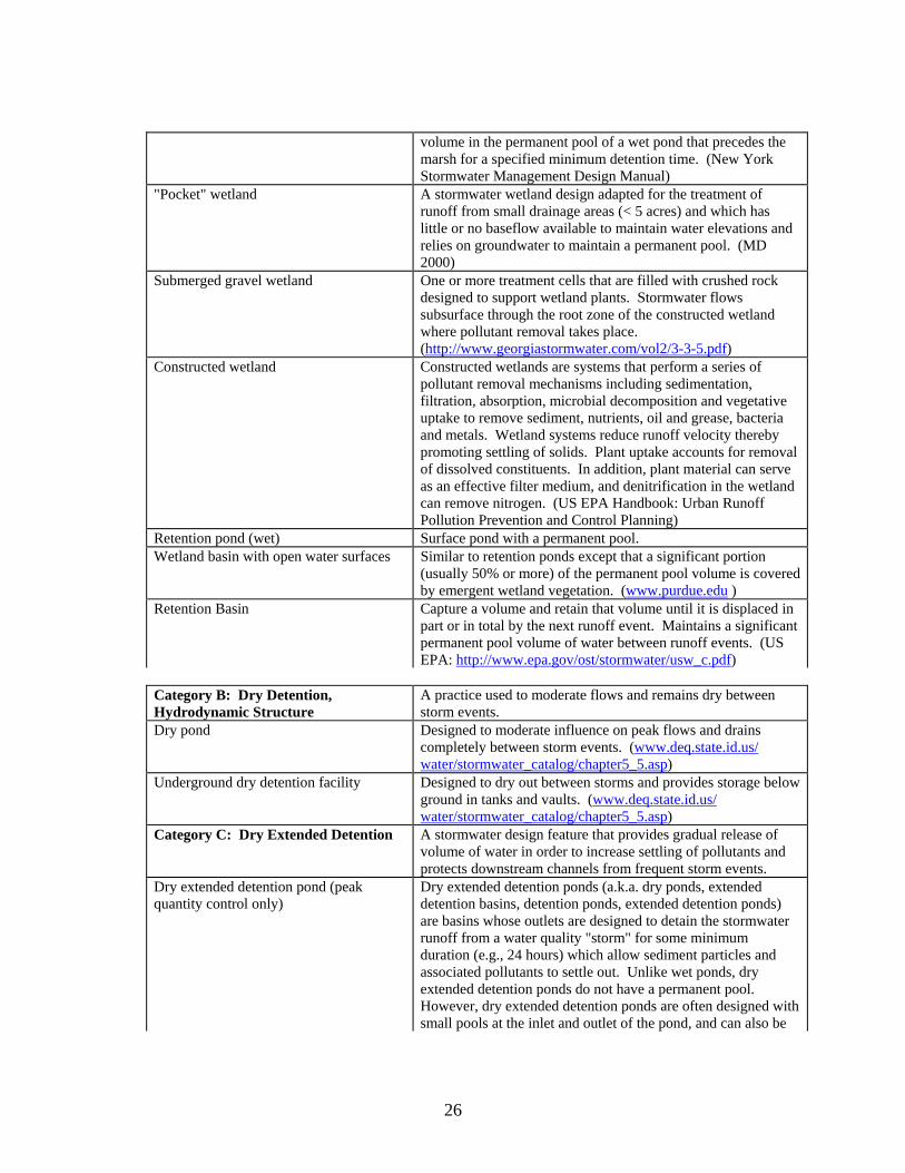
volume in the permanent pool of a wet pond that precedes the marsh for a specified minimum detention time. (New York Stormwater Management Design Manual)

"Pocket" wetland A stormwater wetland design adapted for the treatment of runoff from small drainage areas (< 5 acres) and which has little or no baseflow available to maintain water elevations and relies on groundwater to maintain a permanent pool. (MD 2000)

Submerged gravel wetland One or more treatment cells that are filled with crushed rock designed to support wetland plants. Stormwater flows subsurface through the root zone of the constructed wetland where pollutant removal takes place. (http://www.georgiastormwater.com/vol2/3-3-5.pdf)

Constructed wetland Constructed wetlands are systems that perform a series of pollutant removal mechanisms including sedimentation, filtration, absorption, microbial decomposition and vegetative uptake to remove sediment, nutrients, oil and grease, bacteria and metals. Wetland systems reduce runoff velocity thereby promoting settling of solids. Plant uptake accounts for removal of dissolved constituents. In addition, plant material can serve as an effective filter medium, and denitrification in the wetland can remove nitrogen. (US EPA Handbook: Urban Runoff Pollution Prevention and Control Planning)

Retention pond (wet) Surface pond with a permanent pool. Wetland basin with open water surfaces Similar to retention ponds except that a significant portion

(usually 50% or more) of the permanent pool volume is covered by emergent wetland vegetation. (www.purdue.edu )

Retention Basin Capture a volume and retain that volume until it is displaced in part or in total by the next runoff event. Maintains a significant permanent pool volume of water between runoff events. (US EPA: http://www.epa.gov/ost/stormwater/usw_c.pdf)

Category B: Dry Detention, Hydrodynamic Structure

A practice used to moderate flows and remains dry between storm events.

Dry pond Designed to moderate influence on peak flows and drains completely between storm events. (www.deq.state.id.us/ water/stormwater_catalog/chapter5_5.asp)

Underground dry detention facility Designed to dry out between storms and provides storage below ground in tanks and vaults. (www.deq.state.id.us/ water/stormwater_catalog/chapter5_5.asp)

Category C: Dry Extended Detention A stormwater design feature that provides gradual release of volume of water in order to increase settling of pollutants and protects downstream channels from frequent storm events.

Dry extended detention pond (peak quantity control only)

Dry extended detention ponds (a.k.a. dry ponds, extended detention basins, detention ponds, extended detention ponds) are basins whose outlets are designed to detain the stormwater runoff from a water quality "storm" for some minimum duration (e.g., 24 hours) which allow sediment particles and associated pollutants to settle out. Unlike wet ponds, dry extended detention ponds do not have a permanent pool. However, dry extended detention ponds are often designed with small pools at the inlet and outlet of the pond, and can also be

26

used to provide flood control by including additional detention storage above the extended detention level. (www.stormwatercenter.net)

Extended detention basin An impoundment that temporarily stores runoff for a specified period and discharges it through a hydraulic outlet structure to a downstream conveyance system. An extended detention basin is usually dry during non-rainfall periods. (VA DCR website)

Enhanced extended detention basin An enhanced extended detention basin has a higher efficiency than an extended detention basin because it incorporates a shallow marsh in the bottom. The shallow marsh provides additional pollutant removal and helps to reduce the resuspension of settled pollutants by trapping them. (VA DCR website)

Group D: Infiltration Practices Practices that capture and temporarily store the water quality volume before allowing it to infiltrate into the soil. (MD 2000)

Infiltration Trench An excavated trench that has been back filled with stone to form a subsurface basin. Storm water runoff is diverted into a trench and stored until it can be infiltrated into the soil. (Prince George’s, LID Report)

Infiltration Basin Relatively large, open depressions produced by either natural site topography or excavation. When runoff enters an infiltration basin, the water percolates through the bottom or the sides and the sediment is trapped in the basin. The soil where an infiltration basin is built must be permeable enough to provide adequate infiltration. Some pollutants other than sediment are also removed in infiltration basins. (www.epa.gov/owow/nps/education/runoff.html)

Porous Pavement Pavement that allows stormwater to infiltrate into underlying soils promoting pollutant treatment and recharge. (US EPA LID Fact Sheet)

Category E: Filtering Practices Practices that capture and temporarily store the water quality volume and pass it through a filter bed.

Filtering and Open Channel Practices Practices that capture and temporarily store the water quality volume and pass it through a filter bed of sand, organic matter, soil or other media are considered to be filtering practices. Filtered runoff may be collected and returned to the conveyance system. Vegetated open channels that are explicitly designed to capture and treat the full water quality volume within dry or wet cells formed by checkdams or other means. (MD 2000)

Surface sand filter Both the filter bed and the sediment chamber are above ground. The surface sand filter is designed as an off-line practice, where only the water quality volume is directed to the filter. (www.stormwatercenter.net)

Underground sand filter A modification of the surface sand filter, where all of the filter components are underground. An off-line system that receives only the smaller water quality events. (www.stormwatercenter.net)

27

Perimeter sand filter Includes the basic design elements of a sediment chamber and a filter bed. In this design, however, flow enters the system through grates, usually at the edge of a parking lot. The perimeter sand filter is the only filtering option that is on-line, with all flows entering the system, but larger events bypassing treatment by entering an overflow chamber. (www.stormwatercenter.net)

Organic media filter Essentially the same as surface filters, with the sand media replaced with or supplemented with another medium. The assumption is that these systems will have enhanced pollutant removal for many compounds due to the increased cation exchange capacity achieved by increasing the organic matter. (www.stormwatercenter.net)

Pocket sand filter Diverts runoff from the water quality volume into the filter by pipe where pretreatment is by means of concrete flow spreader, a grass filter strip and a plunge pool. The filter bed is comprised of a shallow basin containing the sand filter medium. The filter surface is a layer of soil and a grass cover. In order to avoid clogging the filter has a pea gravel "window” which directs runoff into the sand and a cleanout and observation well. (http://www.wcc.nrcs.usda.gov/watershed/UrbanBMPs/pdf/water/quality/pocketsandfilter.pdf)

Bioretention areas (a.k.a. Rain Gardens) Primarily for water quality control. These are planting areas installed in shallow basins in which the stormwater runoff is treated by filtering through the bed components, biological and biochemical reactions within the soil matrix and around the root zones of the plants and infiltration into the underlying soil strata (Virginia web site).

Swale In general, a swale (grass channel, dry swale, wet swale, water quality swale) refers to a series of vegetated open channel management practices designed specifically to treat and attenuate stormwater runoff for a specified water quality volume. It is treated through filtering by the vegetation in the channel, filtering through a subsoil matrix, and/or infiltration into the underlying soils. (US EPA Fact Sheet)

Dry Swale A type of grassed swale. Controls quality AND volume (Prince George’s LID). An open drainage channel explicitly designed to detain and promote the filtration of stormwater runoff through an underlying fabricated soil media. (MD 2000)

Infiltration Swale Planted areas designed specifically to accept runoff from impervious areas (i.e. parking lots) providing temporary storage and onsite infiltration. (http://www.metrocouncil.org/environment/Watershed/bmp/CH3_RPPImpParking.pdf)

Wet Swale (a.k.a. Water Quality Swale)

A type of grassed swale. Uses residence time and natural growth to reduce peak discharge and provide water quality treatment before discharge to a downstream location (Prince George’s LID). An open drainage channel or depression, explicitly designed to retain water or intercept groundwater for water quality treatment. (MD 2000)

Dry Wells Dry well – small excavated pit, backfilled with aggregate,

28

usually pea gravel or stone. Function as infiltration systems used to control runoff from building rooftops (Prince George’s LID).

Category F: Roadway Systems (sheet flow to median)

Using a BMP to reduce the total area of impervious cover, thereby reducing the pollutant and sediment load in a given area.

Sheet flow discharge to stream buffers Sheet flow is water flowing in a thin layer of the ground surface. Filter strips are a strip of permanent vegetation above ponds, diversions and other structures to retard the flow of runoff, causing deposition of transported material, thereby reducing sedimentation. (MD 2000)

Category G: Impervious Surface Reduction

Using a BMP to reduce the total area impervious area and therefore encouraging stormwater infiltration.

Natural area conservation Maintaining areas such as forests, grasslands and meadows that encourage stormwater infiltration.

Disconnection of rooftop runoff Disconnecting the rooftop drainage pipe and allowing it to infiltrate into the pervious surface thereby reducing the impervious area.

Disconnection of non-rooftop impervious area

Directing sheet flow from impervious surfaces, i.e. driveways and sidewalks, to pervious surfaces instead of stormwater drains.

Rain Barrels Rain barrels retain a predetermined volume of rooftop runoff (Prince George’s LID).

Green Roofs A multi-layer construction material consisting of a vegetative layer that effectively reduces urban stormwater runoff by reducing the percentage of impervious surfaces in urban areas. (US EPA LID Fact Sheet)

Category H; Street Sweeping, Catch Basin Inserts

A variety of BMPs that provide stormwater treatment for trash, litter, coarse sediment, oil and other debris before proceeding through the stormwater system.

On-line storage in the storm drain network

A management system designed to control stormwater in the storm drain network. (MD 2000)

Catch basin inserts Small, passive, gravity-powered devices that are fitted below the grate of a drain inlet. Intercept and contain significant amounts of litter, vegetation, petroleum hydrocarbons and coarse sediments. (www.kristar.com)

Oil/grit separators Oil/grit separators – systems designed to remove trash, debris and some amount of sediment, oil and grease from stormwater runoff based on the principles of sedimentation for the grit and phase separation for the oil. (www.metrocouncil.org/environment/watershed/bmp/CH3_STDetOilGrit.pdf)

Hydrodynamic Structures A variety of products for stormwater inlets known as swirl separators, or hydrodynamic structures are modifications of the traditional oil-grit separator and include an internal component that creates a swirling motion as stormwater flows through a cylindrical chamber. These designs allow sediment to settle out as stormwater moves in this swirling path. Additional compartments or chambers are sometimes present to trap oil and other floatables. (www.epa.gov/npdes/stormwater/menuofbmps)

Water quality inlets Also known as oil and grit separators, provide removal of

29

floatable wastes and suspended solids through the use of a series of settling chambers and separation baffles. (US EPA Handbook: Urban Runoff Pollution Prevention and Control Planning)

Street sweeping Seeks to remove the buildup of pollutants that have been deposited along the street or curb, using a vacuum assisted sweeper truck.

Deep sump catch basins Storm drain systems designed to catch debris and coarse sediment. (www.lapa-west.org/NPSPollution3.pdf)

Category I: Stream Restoration A BMP used to restore the natural ecosystem by restoring the stream hydrology and natural landscape.

Stream Restoration Return of an ecosystem to a close approximation of its condition prior to disturbance. The establishment of predisturbance aquatic functions and related physical, chemical and biological characteristics. A holistic process. (NRC, 1999, Restoration of Aquatic ecosystems www.epa.gov/owow/)

Impact

The USWG compiled data on the pollutant removal efficiencies of commonly employed urban stormwater management BMPs. Based on BMP pollutant removal efficiencies and general hydrologic effects, these BMPs were grouped into nine categories. It is important to note that this landuse approach applies only to modeling the hydrologic effect of the urban BMPs. The pollutant load reductions of the urban BMPs will be modeled using the pollutant removal efficiencies that have been assigned to each BMP category. Confidence Limits:

It’s important to note the studies on BMP pollutant removal efficiencies are variable and oftentimes scarce. Additionally, many factors affect performance of BMPs, such as the design, frequency of inspection and maintenance, seasonality, and the life span and age of the BMP. Given these uncertainties, the USWG rounded its estimates to the nearest 5 percent.

The USWG did not fully account for changes in pollutant removal efficiencies based on the level of BMP maintenance and the life span of the BMPs. Due to lack of data on stormwater maintenance programs in the watershed, the group was unable to use a “multiplier” to account for reductions in efficiencies due to insufficient maintenance. However, the USWG did not neglect maintenance altogether. Many of the studies evaluated for this effort focused on BMPs that were not regularly maintained. Therefore, the efficiencies, in part, may reflect some lower reduction of pollutant loads due to insufficient maintenance. However, the BMPs are fairly “young” and, therefore, probably do not fully account for reductions in pollutant removal efficiencies due to aging BMPs.

The USWG decided not to include Low Impact Development (LID) or Environmental Site Design (ESD) as a BMP category because no jurisdiction is reporting the number of acres under ESD or LID yet. Jurisdictions are reporting number of acres

30

under certain BMP practices that can be considered a component of ESD or LID, such as bioretention or rooftop disconnection. These practices are already accounted for in the nine BMP categories. The CBP supports the use of ESD and LID and has committed to implement these types of approaches on public-owned lands in the 2001 Storm Water Directive. When localities decide to report their practices in terms of number of acres under ESD or LID, the USWG will develop a list of criteria for ESD/LID and a refined pollutant removal efficiency. It is important to note the workgroup has already developed a pollutant removal efficiency for ESD and LID for the CBP’s Use Attainability Analysis. The efficiencies are TN = 50 percent, TP = 60 percent, and TSS = 90 percent. These efficiencies were chosen based on literature values from the 2000 Maryland Stormwater Design Manual, the Prince George’s County Low-Impact Development Design Strategies manual, and US EPA’s Menu of BMPs that was designed to help localities chose BMPs for implementing the NPDES stormwater regulations.

Treatment trains are a number of BMPs that are connected in series to treat the same volume of runoff. The USWG has concluded that there is not enough hard data to account for pollutant removal efficiencies for “treatment trains”. Funding opportunities to obtain literature and field data are currently being pursued.

Figure 10 summarizes the pollutant removal efficiencies (TN, TP, and TSS) for each of the BMP categories. It is important to note that these pollutant removal efficiencies apply to reductions of loads to surface waters only. Furthermore, these efficiencies are meant for modeling purposes and not for the design and construction of BMPs. Figure 10 Pollutant removal efficiencies for Chesapeake Bay Program urban stormwater BMP categories.

% Pollutant Removal Efficiency Category

TN TP TSS

Comments

Category A:Wet Ponds and Wetlands

30 50 80 This category includes practices such as wet ponds, wet extended detention ponds, retention ponds, pond/wetland systems, shallow wetlands, and constructed wetlands.

Category B:Dry Detention Ponds and Hydrodynamic Structures

5 10 10 Hydrodynamic structures are not considered a stand alone BMP. It acts similar to a dry detention pond and therefore it is included in this group.

Category C:Dry Extended Detention Ponds

30 20 60 This category includes practices such as dry extended detention ponds and extended detention basins.

31

% Pollutant Removal Efficiency Category

TN TP TSS

Comments

Category D: Infiltration Practices

50* 70* 90* This category includes practices such as infiltration trenches, infiltration basins, and porous pavement that reduce or eliminate the runoff. *These efficiencies are based on limited studies.

Category E: Filtering Practices

40 60 85 This category includes swales (dry, wet, infiltration, and water quality), open channel practices, and bioretention that transmit runoff through a filter medium. Grass swales were excluded because they have minimal water quality benefits.

Category F:Roadway Systems

TBD TBD TBD We acknowledge that roadways make up a large portion of the urban acreage in the watershed and that there are practices that are on the ground today that result in some water quality benefit. Due to lack of data, the workgroup has not assigned pollutant removal efficiencies to this category. Your data will help the workgroup to develop an approach for crediting these BMPs

Category G:Impervious Surface Reduction

Model Generated

Model Generated

Model Generated

This category includes a number of practices that essentially turn impervious surfaces into pervious surfaces. Examples of these practices are green roofs, disconnected roofs, rain barrels, removal of impervious surfaces. Pollutant load reductions will be modeled based on the conversion of impervious surfaces to pervious urban surfaces.

Category H:Street Sweeping and Catch Basin Inserts

TBD TBD TBD This category includes municipal efforts such as street sweeping, catch basins cleaning that prevent pollutant loads from entering the Bay. Please provide the number of pounds of TN, TP, and/or TSS removed through these practices.

32

% Pollutant Removal Efficiency Category

TN TP TSS

Comments

Category I:Stream Restoration

0.02 lb/linear ft

0.0035 lb/linear ft

2.55 lb/linear ft

These numbers are based on a study conducted on Spring Branch Stream, an urban watershed in Baltimore County. The Urban Stormwater Workgroup will work with other stream restoration experts to refine these efficiencies, as data become available and to develop criteria for what constitutes water quality-based stream restoration. Please provide details on the types of stream restorations activities you undertook.

Cost Estimations

In October 2003, the CBP published the Technical Support Document for the Identification of Chesapeake Bay Designated Uses and Attainability, which detailed urban stormwater management cost information. The cost analyses indicate that implementing environmental site design or low impact development measures on new development is very inexpensive when compared to the cost of implementing conventional stormwater management practices. When innovative stormwater management practices are used on new developments, the costs are oftentimes completely offset by avoiding the costs for conventional stormwater management infrastructure (i.e., pipes, curbs, etc.). However, retrofitting areas that are already developed to better control stormwater runoff can be very costly. These urban retrofit costs increase even more in ultra-urban areas. The CBP report summarizes some of the latest cost estimates for urban retrofits.

The Chesapeake Bay Watershed Blue Ribbon Finance Panel was established to identify funding sources sufficient to implement basin-wide clean up plans. The Panel learned that current state and local strategies to address all stormwater pollution would cost approximately $15 billion to implement. About 60 percent of this cost estimate, approximately $9 billion, is for retrofitting stormwater management structures in developed areas. This large cost is another reminder that investments in stormwater management prevention and planned growth are more cost effective than repairing the damage once it’s caused (Saving a National Treasure: Financing the Cleanup of the Chesapeake Bay 2004). Implementation

Figure 11 illustrates jurisdictional progress for all types of urban stormwater management implementation with respect to their tributary strategy goal. Tributary strategies outline how the Bay states and the District of Columbia will develop and

33

implement a series of BMPs to minimize pollution. Each river-specific cleanup strategy is tailored to that specific part of the Bay watershed. Data represents implementation levels reported to the CBP, and is taken from the CBP’s Final 2004 Annual Model Assessment (available online at http://www.chesapeakebay.net/tribtools.htm). Urban stormwater management Jurisdiction 2004 Progress (acres) Tributary Strategy Goal (acres) MD 144,583 615,617 PA 0** 752,421 NY 0** 25,616* DE 1,942 3,782* VA 22,758 712,342 WV 24,330 53,494 DC 1,023 26,837 Figure 11 Urban stormwater management implementation levels, for all BMP categories, by jurisdiction. Source: CBP. *Draft tributary strategy. **Tracking/reporting issue Limits to Implementation Cost is the single largest barrier to widespread and effective urban stormwater management. Specifically, the high cost of retrofit continues to remain an obstacle to many local governments, especially as no clear funding source currently exists for capital improvements for stormwater retrofits. According to the Blue Ribbon Panel, funding urban retrofits has generally remained beyond the capabilities of local governments. The Scientific and Technical Advisory Committee held three workshops in October 2002 that examined the impediments to low impact development and environmental site design. The compiled proceedings of all three workshops, including a summary list of the most important impediments, are available at http://www.chesapeake.org/stac/Pubs/ILIDFinalReport.PDF. In 2003, Virginia DCR and DEQ hosted five workshops throughout the commonwealth to introduce low impact development to and obtain comments from the public on implementation of LID. A summary of the proceedings, including impediments to implementation, is available online at http://www.nao.usace.army.mil/Regulatory/LID_workshop_report.pdf. BMP Tracking/Reporting

For CBP guidelines on reporting urban stormwater BMP data, see the document, BMP Guidance for the States and the District.

The Bay watershed states and US EPA Region III are working to tie in tracking efforts into stormwater permits (both Phase II and Phase I reissued permits) to provide the key data needed by the Bay program to credit jurisdictions for their stormwater management activities. The USWG is working to determine a way to estimate the level of urban

34

stormwater BMPs that were implemented prior to 2000. Much of that data does not exist in electronic format or was never compiled. Possible Funding Sources/Implementation Opportunities

Stormwater management projects are eligible for funding under the State Revolving Loan Fund Program and the Section 319 Nonpoint Source Program of the Clean Water Act. Unfortunately, these funds are inadequate to the need. The Blue Ribbon Panel noted that developers and buyers might absorb the capital costs of incorporating stormwater controls into new development. Furthermore, localities can implement programs such as stormwater utility fee systems to enforce stormwater pollution prevention requirements and to inspect, operate and maintain BMPs. However, no clear funding source currently exists for capital improvements for stormwater retrofits. Given that retrofits account for roughly 60 percent of the estimated stormwater pollution control costs, the estimated funding gap is about $9 billion.

Builders for the Bay is a first-of-its-kind program aimed at reducing environmental impacts from residential and commercial construction within the Chesapeake Bay watershed. Officially signed on December 3, 2001, Builders for the Bay is an agreement among the Center for Watershed Protection, the Alliance for the Chesapeake Bay, and the National Association of Home Builders to pursue 12 local site planning roundtables in the Chesapeake Bay watershed over the next several years. The local site planning roundtables are a consensus process through which jurisdictions actually change existing local subdivision codes and ordinances to be more environmentally friendly and economically prudent. By making it easier for communities to implement Better Site Design, the goal is to ultimately preserve and enhance more natural areas; reduce and manage the amount of stormwater that flows off of a development site; and save developers money. Since the Builders for the Bay agreement was signed, the Maryland State Builders Association, the Home Builders Association of Virginia, the Pennsylvania Builders Association and their local affiliates, and interested local governments have all become partners in the program and will have substantive roles in moving the local roundtables forward. More information is available at their website, http://www.cwp.org/builders_for_bay.htm. Notes on Modeling the BMP

The CBP watershed model credits stormwater BMPs as detailed in Figure 10, page 25.

The current watershed model, Phase 4.3, does not account for reductions in pollutant loads that may result from hydrologic effects of the urban stormwater BMPs. In reality, many urban stormwater BMPs reduce peak runoff flows and volumes, and increase time of concentration. When peak runoff flows are reduced, stream flow velocities are reduced, which may result in reduced stream bank erosion. Currently, the model does not account for reductions in sediment loads from reduced stream bank erosion that may result from urban stormwater BMP implementation. The USWG is working with the CBP’s Modeling Team to model pollutant loads resulting from hydrologic changes from urban BMPs. Note that watershed model 4.3 does not capture

35

any stream smaller than third order, thus cannot model the hydrologic effects of stormwater BMPs on first and second order streams. References ASCE National BMP Database. http://www.bmpdatabase.org/. Center for Watershed Protection’s National Pollutant Removal Performance Database for Stormwater Treatment Practices 2000 Maryland Stormwater Design Manual. http://www.mde.state.md.us/Programs/WaterPrograms/SedimentandStormwater/stormwater_design/index.asp Virginia Stormwater Handbook. http://www.dcr.virginia.gov/sw/stormwat.htm Low-Impact Development Design Strategies: An Integrated Design Approach. Prepared by Prince George's County, Maryland, Department of Environmental Resources, Programs and Planning Division; June 1999. Saving a National Treasure: Financing the Cleanup of the Chesapeake Bay. Chesapeake Bay Program’s Blue Ribbon Panel Report, October 2004. http://www.chesapeakebay.net/pubs/blueribbon/index.cfm District of Columbia’s Department of Health – BMPs in Anacostia River Watershed

36

STRUCTURAL SHORELINE EROSION CONTROLS Presented by Lee Hill from the Virginia Department of Conservation and Recreation BMP Definitions

Structural shoreline erosion controls are designed to protect eroding shorelines by armoring the shoreline to dissipate incoming wave energy while protecting unconsolidated bank sediments. These practices are applicable in areas of higher erosion rates or where wave energy is too strong for vegetative alternatives.

Four structural shoreline erosion control BMPs were presented at the workshop. Each is defined in this section. • Shoreline “hardening”

These projects are rigid, barrier-type structures that result in a “hardening” of the shoreline to protect against the action of waves, currents, tides, wind driven water, runoff from storms, and/or groundwater seepage that erodes shorelines. Such structural measures include, but are not limited to: riprap, revetments, bulkheads, groins (built perpendicular to the shoreline to trap sand, also known as a jetty), and seawalls.

Figure 12 Stone revetment on the Potomac River, Virginia.

37

• Offshore Breakwaters An offshore breakwater is a structure positioned a short distance from the shore to deflect the force of incoming waves to protect the shoreline.

Figure 13 Offshore breakwater. • Headland Controls

A headland control is a structure that creates or protects an erosion resistant point or points of land, allowing adjacent embayments to achieve a stable configuration.

Figure 14 Headland control system using widely spaced breakwaters on Hog Island, James River, Virginia.

38

• Breakwater Systems Also known as living shorelines, breakwater systems are a combination of structures, practices and vegetative measures, including beach nourishment, wetlands and dune plantings that are positioned along a shore to deflect and dissipate the force of waves in order to protect the shoreline. In the 2005 report Sediment in the Chesapeake Bay and Management Issues: Tidal Erosion Processes, the CBP’s SedWG recommends living shorelines for areas experiencing erosion of two feet per year or less.

Figure 15 Typical cross-section of a breakwater system. Source: Hardaway and Byrne, 1999. Impact

Depending on the design, structural shoreline erosion controls can help shorelines withstand wave impact, retain the protected earth on the bank, trap sand, and, in general, may very effectively prevent fastland erosion at the site of protection.

However, it must be noted that structural shoreline erosion controls may inhibit the shoreline’s natural evolution. In the absence of shoreline erosion controls, the natural response of beaches and tidal wetlands to fastland erosion would be a migration inland. Hardened shorelines may limit the shoreline’s ability to migrate while effectively starving adjacent beaches and wetlands of necessary sediment inputs. Furthermore, hard shoreline protection structures may increase bottom scour and erosion in the nearshore zone in front of the structures because they tend to reflect the oncoming wave energy (Army Corps of Engineers 2002). They also may decrease the diversity and quality of habitats on both sides of the structure and impede those natural processes that are necessary and beneficial for healthy aquatic ecosystems. Sediment Reduction Efficiency

Lee Hill recommends that if bank stability was the only consideration in the efficiency, a value of 90 – 100 percent could be assigned to the shoreline hardening BMP. If bank stability, beach scour and adjacent and downdrift impacts are considered in the efficiency, a value of 50 – 75 percent could be assigned; however, the adjacent and downdrift impacts of properly designed and constructed measures is not well documented. When reporting sediment and nutrient savings for implemented shoreline erosion control measures for Virginia tributary strategy reports, an efficiency of 75 percent was used.

39

The efficiency of a breakwater is site specific. Breakwaters installed along a shoreline protect a portion of the shore from erosion, while the unprotected segments may continue to erode. The eroded material is deposited behind the breakwater and builds a protective beach. Over time, this erosion – deposition cycle continues until the area reaches a state of equilibrium. Once equilibrium is achieved, the erosion – deposition cycle is balanced and the entire project area is protected. Therefore, the efficiency over time varies. In addition, the project may have adjacent and downdrift impacts. Therefore, the efficiency varies. Lee’s recommended reporting efficiency is 40 percent sediment reduction for offshore breakwaters.

The implementation of a breakwater system is effective in protecting the shoreline from erosion and minimizes adjacent and downdrift impacts. The utilization of beach nourishment in conjunction with wetlands and dune plantings eliminates the erosion/deposition cycle associated with the use of breakwaters alone. Therefore, the efficiency is 90 – 100 percent for beach nourishment in conjunction with wetlands and dune plantings. When reporting sediment and nutrient savings for implemented shoreline erosion control measures for tributary strategy reporting, an efficiency of 75 percent was used in Virginia’s tributary strategies.

Headland controls allow for long stretches of shoreline to be protected with a minimum of structures. As with breakwaters, selected points are protected and the land between the points is allowed to erode. Ideally, over time, equilibrium is reached and a stable embayment is created. Therefore, the efficiency of the headland control practice varies as time progresses with the formation of the stable embayment. When equilibrium is reached, the efficiency is 90 – 100 percent. For modeling purposes, the recommendation is to use an efficiency of 50 percent for the life of the measure. Nutrient Reduction Efficiency

The nutrient reduction efficiency of structural shoreline erosion controls is related to the sediment control efficiency, as the sediments controlled by the BMP have associated nutrients. Using the report entitled “Eroding Bank Nutrient Verification Study for the Lower Chesapeake Bay” by Ibison, et al. (1992), a nutrient savings could be calculated for the practice. Cost Estimations

Costs of structural shoreline erosion controls range from $50 - $400 per linear foot of protected shoreline. Headland controls are significantly less expensive than other structural controls, and may enable landowners and jurisdictions to protect “less-valued” lands along the Bay and major tributaries. Implementation

Structural shoreline erosion controls have applicability in the Bay and the major tributaries.

40

Limits to Implementation The cost of structural shoreline erosion controls limits their implementation. Private landowners control approximately 85 percent of Chesapeake shoreline (Claggett, 2005), and bear the majority of the financial burden for erosion controls.

Often shorelines are unnecessarily hardened in areas that have low erosion rates. In fact, hardened shorelines may increase nearshore erosion. In areas experiencing erosion of two feet or less per year, the CBP recommends nonstructural shore erosion controls, also known as living shorelines, which create protective vegetative buffers and habitat (Tidal Erosion Processes 2005). Furthermore, there are eroding shorelines where no action should be taken if the eroded shorelines are replenishing beaches or providing a unique habitat for endangered species. It is imperative that decision makers and landowners understand the nuances and long-term benefits and effects of shoreline management. BMP Tracking/Reporting

Implementation of the Structural Control BMP can be tracked through the permitting process of the Army Corps of Engineers (USACE) and the individual jurisdictions. Based on the permitted length of the project, a sediment and nutrient reduction load can be calculated for the practice. The reductions can then be assigned to the segments of the model where the practice was implemented. The individual jurisdictions would be responsible for reporting the savings associated with the practice. Possible Funding Sources/Implementation Opportunities

At the present time, private landowners pay for the majority of the projects utilizing the Structural Shoreline Control BMP. One option to enhance the use of the BMP is to create a Shoreline Erosion Control Cost-Share Program and include the practice as one of the measures in the program.

The NOAA Restoration Center provides financial and technical assistance for estuarine and riparian habitat restoration projects that restore and stabilize eroding shorelines throughout the Chesapeake Bay watershed. In 2004, NOAA, the Chesapeake Bay Foundation, the Keith Campbell Foundation for the Environment and the National Fish and Wildlife Foundation created a partnership to fund living shoreline restoration projects in Maryland and Virginia. For more information on NOAA funding opportunities contact Alison Ward Maksym (410 267 5644; alison.ward-maksym@noaa.gov) or Rich Takacs (410 267 5672; rich.takacs@noaa.gov) at the NOAA Restoration Center. Additional information on funding availability can be found at http://www.nmfs.noaa.gov/habitat/restoration/funding_opportunities/funding.html.

In Virginia, the Department of Conservation and Recreation provides waterfront property owners with free assistance about how to protect eroding shorelines. In Maryland, two agencies within the Department of Natural Resources provide waterfront property owners with free technical and financial assistance: the Coastal Zone Management Program, and the Shore Erosion Control Program. The Shore Erosion Control Program provides technical and financial assistance to Maryland property owners in resolving shoreline and streambank erosion problems. Financial assistance as loans for

41

structural projects is now available for municipality, county, and county-sponsored projects. Notes on Modeling the BMP

In the event that progress assessments were run, the CBP could currently credit all structural and non-structural shoreline erosion controls in Maryland and Virginia with a sediment reduction value of 2.917 kg/day/ft, to be applied in the water quality model. This efficiency is based on assumptions of Maryland Department of Natural Resources data. The reductions provided by this practice can be assigned to the segments of the model where the practice is implemented. Maintenance plans should be in place to ensure the BMP maintains the efficiency stated at the time it was installed. The efficiencies may need to be reduced over time. References Hardaway, C.S. and R. J. Byrne. 1999. Shoreline Management In Chesapeake Bay. Virginia Sea Grant Publication VSG-99-11. Claggett, P. Personal Communication November 2004. Chesapeake Bay Program Office, Annapolis, MD The Chesapeake Bay Program’s Sediment Workgroup. Sediment in the Chesapeake Bay and Management Issues: Tidal Erosion Processes. May 2005. http://www.chesapeakebay.net/pubs/doc-tidalerosionChesBay.pdf. The Virginia Wetlands Report. Summer 2004 Vol. 19, No. 2 Titus, J. 1998. Rising Seas, Coastal Erosion and the Taking Clause: How to Save Wetlands and Beaches Without Hurting Property Owners. Maryland Law Review, Volume 57, number 4. p. 1281-1399. U.S. Army Corps of Engineers. 2002. Coastal Engineering Manual: U.S. Army Corps of Engineers, 1110-2-1100. Ibison, N.A., J.C. Baumer, C.L. Hill, N.H. Burger, and J.E. Frye. 1992. Eroding Bank Nutrient Verification Study for the Lower Chesapeake Bay. Virginia Department of Conservation and Recreation, Gloucester Point, Virginia. Ibison, N.A., C.W. Frye, J.E. Frye, C.L. Hill, and N.H. Burger. 1990. Sediment and Nutrient Contributions of Selected Eroding Banks of the Chesapeake Bay Estuarine System. Virginia Department of Conservation and Recreation, Gloucester Point, Virginia.

42

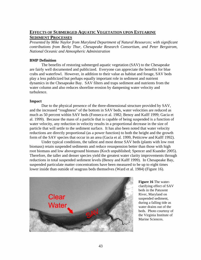
EFFECTS OF SUBMERGED AQUATIC VEGETATION UPON ESTUARINE SEDIMENT PROCESSES Presented by Mike Naylor from Maryland Department of Natural Resources; with significant contributions from Becky Thur, Chesapeake Research Consortium, and Peter Bergstrom, National Oceanic and Atmospheric Administration BMP Definition

The benefits of restoring submerged aquatic vegetation (SAV) to the Chesapeake are fairly well documented and publicized. Everyone can appreciate the benefits for blue crabs and waterfowl. However, in addition to their value as habitat and forage, SAV beds play a less publicized but perhaps equally important role in sediment and nutrient dynamics in the Chesapeake Bay. SAV filters and traps sediment and nutrients from the water column and also reduces shoreline erosion by dampening water velocity and turbulence. Impact

Due to the physical presence of the three-dimensional structure provided by SAV, and the increased “roughness” of the bottom in SAV beds, water velocities are reduced as much as 50 percent within SAV beds (Fonseca et al. 1982; Benoy and Kalff 1999; Gacia et al. 1999). Because the mass of a particle that is capable of being suspended is a function of water velocity, any reduction in velocity results in a proportional decrease in the size of particle that will settle to the sediment surface. It has also been noted that water velocity reductions are directly proportional (as a power function) to both the height and the growth form of the SAV species that occur in an area (Gacia et al. 1999, Petticrew and Kalff 1992).

Under typical conditions, the tallest and most dense SAV beds (plants with low root biomass) retain suspended sediments and reduce resuspension better than those with high root biomass and low aboveground biomass (Koch unpublished; Spencer and Ksander 2005). Therefore, the taller and denser species yield the greatest water clarity improvements through reductions in total suspended sediment levels (Benoy and Kalff 1999). In Chesapeake Bay, suspended particulate matter concentrations have been measured to be up to eight times lower inside than outside of seagrass beds themselves (Ward et al. 1984) (Figure 16).

Figure 16 The water-clarifying effect of SAV beds in the Patuxent River, Maryland on suspended sediment, during a falling tide as water drains out of the beds. Photo courtesy of the Virginia Institute of Marine Sciences.

43

The potential sediment-related benefits of SAV are outlined below:

1) Increased sedimentation rate within beds

• It has been demonstrated experimentally that SAV beds accumulate sediment at a rate 2 to 20 times greater than that which occurs in the profundal zone (Benoy and Kalff 1999, Gacia et al. 1999), and sediment trapping rates were recorded to be an order of magnitude higher inside SAV beds than in nearby open waters (Ward et al. 1984). These effects are a direct result of the decrease in water velocity described above. Sediment accumulation rates vary as a function of plant biomass, density and growth form, and suspended sediment composition. Canopy forming species intercept more sediment than understory meadow formers (Petticrew and Kalff 1992). Beds of meadow forming species contain a higher proportion of autochthonous sediment (originating within the bed) than canopy forming species, showing that the canopy formers trapped more sediment that originated elsewhere (Benoy and Kalff 1999).

2) Decreased resuspension of sediment from within vegetated areas

• Once sediment has settled from the water column, several factors serve to retain those sediments at a minimum of an order of magnitude higher rate than sediments in unvegetated areas: a. increased bottom roughness associated with SAV beds, b. stabilization of sediment by SAV roots, and c. lower wave energy within beds (Gacia et al. 1999; Benoy and Kalff 1999). It has been noted that, in some cases, disappearance of SAV from areas that were previously stable resulted in “massive” losses of littoral sediments (Schroder 1988). A reduction in shoot density or an increase in water depth (due to tides or storm surge) that subsequently reduces or eliminates the capacity of a bed to attenuate waves can render the underlying sediment more vulnerable to erosion, leading to higher concentrations of suspended sediment particles in the water column (Koch 2001). Plants with high root to shoot ratios retain sediments (and thus reduce resuspension) better than those with lower root biomass (Jaynes and Carpenter 1986). Furthermore, the increased stability of sediments caused by SAV roots can minimize the lateral migration of sediments. In addition to physically retaining sediments, the characteristics of sediment are different within SAV beds than surrounding areas. For example, organic matter mineralization is four times higher in SAV beds than in the pelagic zone (Heyer and Kalff 1998).

44

3) Decreased shoreline erosion due to the dampening of water velocity and turbulence by adjacent SAV beds. • As early as 1975, it was recognized that SAV beds helped to retain sediments, and

plantings were being undertaken specifically to stabilize sediments (Churchill et al. 1978). The processes of reduced wave energy and increased sedimentation work together to facilitate a reduction in shoreline erosion. As waves, generated as a function of wind velocity and fetch, move from open water towards shorelines, near-shore SAV beds that reduce water velocity will reduce wave impact to the shore. This is often directly observable when on the water; choppy water in mid-channel approaching SAV beds is quickly dampened, and the shoreward sides of the beds are often completely calm in all but the most severe wind events. Decreases in the amount of wave energy that reaches the shoreline should reduce erosion caused by waves. The efficiency with which waves are attenuated by SAV beds depends, however, on water depth, current velocity, plant morphology, and the percentage of the water column occupied by the vegetation (Koch 2001). When plants are reproductive and occupy the entire water column, maximum wave attenuation can reach 50 percent (Newell and Koch 2004).

The sediment accumulation that occurs in SAV beds can also reduce shoreline erosion. Increased sedimentation in SAV beds can create shoaling, which causes waves to break earlier and at greater distances from shore, further reducing the amount of energy reaching the shoreline. It should be noted, however, that in SAV beds with high exposure (>10 km fetch), sediment accumulation might be negligible (Benoy and Kalff 1999), presumably due to energy in these areas being great enough to overwhelm the buffering effect provided by SAV.

∗ For most of the Chesapeake Bay, and for nearly all of Maryland, most of these benefits are seasonal in nature, as SAV retain aboveground biomass for only 4-9 months out of the year (Figure 17). Root matter does function to help retain sediments, but not at the same rate as when aboveground biomass is present.

Sediment Reduction Efficiency

Within SAV beds, one can expect a 2 to 20-fold increase in particle settling velocities during the relevant growing seasons for each community. One can expect a doubling of settling velocities in low-density SAV beds, and an increase to the 20-fold level at the most dense, canopy-forming beds. Figure 17 contains data on settling factors relevant to various species of SAV.

45

Community Canopy or meadow forming

Growing season

Plants present

Maximum Particle Settling Reduction Factor

Zostera meadow Mar-May, Sept-Nov

year round x15

Ruppia intermediate May-Oct May-Oct x10

Potamogeton intermediate April-Oct April-Nov x20

Freshwater intermediate April-Oct April-Nov x20 Figure 17 Characteristics of Chesapeake Bay’s SAV communities relevant to estuarine sediment processes (Moore 1999). Nutrient Reduction Efficiency

SAV affects nutrient levels in two ways: by settling and trapping particles, thereby achieving some reduction in TP; and by nutrient uptake directly through leaf tissue during the growing season, releasing most of the nutrients in the fall and early winter as plant tissues break down. The influence of SAV on the timing of nutrient availability can be critical, as nutrient problems such as eutrophication tend to worsen in the summer. Moreover, the uptake of nutrients during the summer is substantial; for instance, SAV is used to remove nutrients from wastewater in third world countries. SAV also promotes denitrification (and reduces nitrification) by transporting oxygen to anoxic regions of the sediment. Cost Estimations

Cost of restoration varies widely depending upon the species used, the planting technique, and the intensity of monitoring. Approximate costs can vary from $5,000 to over $15,000 per acre. Implementation

Nearly 200,000 acres of SAV are estimated to have historically grown in the shallows and along the shorelines of the Chesapeake Bay and its rivers. By 1984, however, only 38,000 acres were documented from aerial surveys. Efforts to restore SAV have increased acreage over time, but in 2003, a total of 64,709 acres of SAV were estimated to be growing in the Bay - a 30 percent decline from the previous year's tally. In 2004, 72,935 acres of SAV were counted in the VIMS annual survey, still 16,720 acres shy of the 2002 acreage.

The CBP has committed significant resources over the past 20 years to determine the causes for the decline and to identify the best methods for protecting and restoring SAV populations. As a result of significant losses in Bay grass acreage, CBP’s Directive 93-3 set a goal of achieving 114,000 acres of Bay grasses, and this goal was reaffirmed in the Chesapeake 2000 agreement. In 2003, CBP partners adopted a new, expanded goal

46

and strategy to accelerate SAV protection and restoration. The goal is to achieve 185,000 total acres of SAV, Bay wide, by the year 2010. The strategy to achieve this goal is based on consensus among the formal and informal partners of the CBP, and its status will be reported annually and reevaluated in 2008. According to the SAV Strategy document, the primary way to achieve the needed increase in SAV area is to improve water clarity; secondary methods include SAV planting and SAV protection.

Considering the threats to SAV survival, BMPs should be piloted in areas of relatively good water quality. There are many regions within the Chesapeake Bay in which habitat conditions are suitable for Bay grass growth, but that currently lack vegetation, probably due to a lack of adequate seed or propagule sources. By identifying and strategically planting or reseeding beds in these areas, it is expected that these beds would serve as a seed source to greatly accelerate natural revegetation on a much larger scale. Additionally, there are many areas of the Chesapeake Bay that are currently vegetated by exotic, or non-native, SAV species such as hydrilla and Eurasion watermilfoil. By establishing native SAV beds in these areas, it is expected that the more beneficial, native species may eventually replace the exotics.

By monitoring SAV in the Chesapeake Bay, biologists can determine which areas need to be protected. By examining historical distribution, areas where SAV once flourished are targeted for restoration. Actual locations of SAV beds can be viewed at http://www.vims.edu/bio/sav. Limits to Implementation

The following three types of impacts (natural events, sediment loading, and various human impacts) cause specific problems for SAV:

1) Natural Impacts

• Hurricanes and lesser storms can cause strong wave action, which can rip up SAV. Large deposits of sediments from these storms can also bury SAV beds, preventing propagation. In June 1972, Hurricane Agnes decimated SAV beds in the Bay. Grasses had not yet seeded or, in the case of several species, even come up yet, when the storm deposited up to 8 feet of sediments in some parts of the Bay as a result of record amounts of rainfall on the watershed (Lynch 2005). Over 31 million metric tons of suspended sediment were discharged into the Bay by the Susquehanna River alone (Hennessee and Halka 2005). It is estimated that this one storm resulted in a loss of 67 percent of the biomass of all species of SAV, with eelgrass being hardest hit (89 percent loss) (Lynch 2005).

• The extent to which periods of abnormally low water clarity impact SAV is

related to its coincidence with the growing season of SAV. For example, a strong mahogany tide in late April - early May 2000 apparently caused a dieback in SAV that year in a number of mesohaline Chesapeake segments (Gallegos and Bergstrom 2004). Conversely, the storm surge of Hurricane Isabel in September 2003 brought high winds and waves with strong currents that resulted in significant amounts of shoreline erosion, but due to the late-summer timing of the

47

storm and its elevated tidal heights, the impact of Isabel on the Bay’s SAV was relatively minimal (Hennessee and Halka 2005; Trice et al. 2005).

• Disease also has the potential to threaten future SAV restoration efforts (Shearer

1994). During the 1930s, wasting disease, caused by the marine slime mold (Labyrinthula zosterae), caused extensive damage to eelgrass populations in many temperate coastal areas, including the lower Chesapeake Bay, and diminished eelgrass coverage by over 90 percent in some areas. It is known that elevated salinities increase the extent of this disease, while reduced salinities (<20-25 ppt, Burdick et al. 1993) suppress its spread. However, the mechanisms of infection, spread, and resistance within individual plants are poorly understood, and as global warming-induced sea level rise elevates temperature and salinity within estuarine systems, the potential for complete elimination of eelgrass due to a combination of plant stress and wasting disease will increase (Short and Neckles 1999).

2) Sediment Composition Impacts

• Grain size (i.e., sand/silt/clay fractions) influences the stability of the sediments and the ability of the sediment to retain nutrients, both of which in turn influence SAV. Larger grain sizes, which are generally less stable and more likely to migrate, can reduce SAV growth by exposing or burying propagules unpredictably, thus decreasing recruitment the following year. Furthermore, larger grain sizes are more nutrient poor and result in plants with more belowground than aboveground biomass, which are less likely to prevent resuspension.

• High organic matter and/or sulfur in the sediments affect SAV directly by creating

unfavorable conditions for roots, and generally results in greater above-ground than below-ground biomass (Van et al. 1999). Some species of SAV have no true roots at all and can tolerate any percentage of organic matter (e.g. Ceratophyllum demersum), while many others will not grow at all if the organic content exceeds approximately five percent (Barko and Smart 1983; Batiuk et al. 2000; Koch 2001). Higher tolerances to organic matter (6.5 – 12 percent) occur mainly in species with larger leaves that have a greater capacity to transport oxygen to their roots, or in areas where sediments in the root zone are otherwise well-oxygenated (Batiuk et al. 2000; Koch 2001).

3) Other Anthropogenic Impacts

• Chemical run-off from the use of fertilizers, herbicides and pesticides can create unfavorable conditions for SAV. Excess nutrients from wastewater treatment plants, urban and agricultural runoff and other activities can lead to eutrophication, causing algae blooms that block light needed for SAV growth. These issues are compounded by human and animal population growth in the watershed, which leads to higher pollutant loads delivered to the Bay. Moreover,

48

invasive species, such as the mute swan, can cause considerable damage to SAV beds by feeding on and uprooting large areas of grasses in short periods of time (AFC 2003). Invasive species may also compete with and displace native species.

BMP Tracking/Reporting

The Virginia Institute of Marine Science (VIMS) monitors Chesapeake SAV distribution each year. By examining aerial photographs, locations, areas, and estimated densities of SAV beds are mapped for the entire Chesapeake Bay and its tidal tributaries. Possible Funding Sources/Implementation Opportunities

Limited, but dedicated funding for SAV restoration work is available through NOAA’s Chesapeake Bay Integrated Research Program for SAV Culture and Restoration (information is available online at http://noaa.chesapeakebay.net/aquaticvegetationgrants.aspx). More general habitat restoration funds, including SAV restoration projects, have also been made available in recent years through various other sources, such as the Fish America Foundation, the Department of Defense Legacy and Strategic Environmental Research & Development (SERDP) Programs, the Chesapeake Bay Trust, the Plant Conservation Alliance, USACE, and the National Fish and Wildlife Foundation. However, the majority of these sources are not strictly dedicated to projects in the Chesapeake, nor do the requests for proposals often specifically target SAV restoration, making successful competition for their funds difficult and unpredictable. Notes on Modeling the BMP

The current Chesapeake Bay water quality model simulates SAV, but no credit is given as a BMP.

To estimate the impact of SAV planting, one could choose a few levels in a ranging exercise and model the effects. SAV planting can be applied annually and spatially for the entire Chesapeake Bay as two-dimensional acreage. This could also be back calibrated through 1985 with near complete coverage. SAV bed coverage already exists as GIS data layers with associated densities for each polygon that would facilitate the application of a multiplier. Furthermore, calculation of potential benefits of a restored SAV community could be easily calculated by applying the single best year SAV coverage, at their respective (or if necessary some representative) density classes, in the manner described above. This would allow a direct calculation of the potential benefits to estuarine sediment processes of SAV planting. The following are descriptions of how the water quality model could incorporate the maximum particle settling factor and calculate the reduction efficiencies for SAV:

• 1Model multiplier for solids settling velocities (Wnet), varying from x2 at bed density of 1 in a meadow forming species, to x20 at bed density of 4 in a canopy forming species, with a maximum set based on the growth form(s) of the relevant communities. Another option would be to relate this to biomass, estimated from visually estimated percent cover. Both techniques would rely upon the VIMS SAV coverage data set. It will be important to take into account that the plants

49

are gone over the winter, at least 5 months per year, except in the case of eelgrass. It is the only species with close to a year-round, aboveground biomass effect.

• 2Model multiplier of -(x10) for reducing resuspension within SAV beds based on

density (if a resuspension algorithm is developed for the model). References Atlantic Flyway Council (AFC). 2003. Atlantic Flyway Mute Swan Management Plan.30 pp. http://www.dnr.state.md.us/wildlife/afcmuteplan.html Benoy, G.A. and Kalff, J. 1999. Sediment accumulation and Pb burdens in submerged macrophytee beds Limnol. Oceanogr., 44(4): 1081-1090. Barko, J.W. and M. Smart. 1983. Effects of organic matter additions to sediment on the growth of aquatic plants. J. Ecol. 71: 161-175. Batiuk, R.A., P. Bergstrom, M. Kemp, E. Koch, L. Murray, J.C. Stevenson, R. Bartleson, V. Carter, N.B. Rybicki, J.M. Landwehr, C. Gallegos, L. Karrh, M. Naylor, D. Wilcox, K.A. Moore, S. Ailstock, and M. Teichburg. 2000. Chesapeake Bay Submerged Aquatic Vegetation Water Quality and Habitat-Based Requirements and Restoration Targets: A Second Technical Synthesis. CBP/TRS 245-00. Chesapeake Bay Program, Annapolis, Maryland. http://www.chesapeakebay. net/pubs/sav/index.html Burdick, D.M., Short, F.T., and Wolf, J. 1993. An index to assess and monitor the progression of wasting disease in eelgrass Zostera marina. Mar. Ecol. Prog. Ser. 94: 83-90. Churchill, A.C., Cok, A.E. and Riner, M.I. 1976. Stabilization of subtidal sediments by the transplantation of the seagrass Zostera marina. Report to New York Sea Grant, NYSSGP-RS-78-15 Fonseca, M.S. and Fisher, J.S. 1986. A comparison of canopy friction and sediment movement between four species of seagrass with reference to their ecology and restoration. Mar. Ecol. Prog. Ser. 29: 15-22. Fonseca, M.S. et al. 1982. Influence of seagrass Zostera marina, on current flow. Estuarine Coastal Shelf Science. 15: 351-364. Gacia, E., Granata, T.C., and Duarte, C.M. 1999. An approach to measurement of particle flux and sediment retention within seagrass meadows. Aquatic Botany. 65: 255-268.

50

Gallegos, C. L., and P. W. Bergstrom. 2004. Effects of a Prorocentrum minimum bloom on light availability for and potential impacts on submersed aquatic vegetation in upper Chesapeake Bay. Harmful Algae 4: 553-574. Ginsberg, R.N. and Lowenstam, H.A. 1958. The influence of marine bottom communities on the depositional environment of sediments. J. Geol. 66: 310-318. Note: this is not referenced in the text. den Heyer, C. and Kalff, J. 1998. Organic matter mineralization rates in sediments: A within and among lake study. Limnol. Oceanogr. 43: 695-705. Hennessee, E.L. and Halka, J.P. 2005. Hurricane Isabel and erosion of Chesapeake Bay shorelines, Maryland. In: K.G. Sellner (ed.). 2005. Hurricane Isabel in Perspective. Chesapeake Research Consortium, CRC Publication 05-160, Edgewater, MD. Jaynes, M.L., and Carpenter, S.R. 1986. Effects of vascular and nonvascular macrophytes on the sediment redox and solute dynamics. Ecology 67: 875-882. Koch, E.W. 2001. Beyond light: physical, geological and geochemical parameters as possible submersed aquatic vegetation habitat requirements. Estuaries 24:1-17. Lynch, M.P. 2005. An unprecedented scientific community response to an unprecedented event: Tropical Storm Agnes and the Chesapeake Bay. In: K.G. Sellner (ed.). 2005. Hurricane Isabel in Perspective. Chesapeake Research Consortium, CRC Publication 05-160, Edgewater, MD. Newell, R.I.E. and E.W. Koch. 2004. Modeling seagrass density and distribution in response to changes in turbidity stemming from bivalve filtration and seagrass sediment stabilization. Estuaries. 27: 793-806. Petticrew, E.L., and Kalff, J. 1991. Predictions of surficial sediment composition in the littoral zone of lakes. Limnol. Oceanogr. 36: 384-392. Schroder, V.R. 1988. Sublittoral erosion of Untersee (Lake Constance): Late consequences of eutrophication and hydrological phenomenon. Arch. Hydrobiologia. 12: 265-277. Scoffin, T.P. 1970. The trapping and binding of subtidal carbonate sediments by marine vegetation in Bimini Lagoon, Bahamas Arch. Hydrobiol. 40: 249-273 Short, F.T., and Neckles, H.A. 1999. The effects of global climate change on seagrasses. Aquat. Bot. 63: 169-196.

51

Spencer, D.F. and G.G. Ksander. 2005. Root size and depth distributions for three species of submersed aquatic plants grown alone or in mixtures: Evidence for nutrient competition. J. Freshwater Ecol. 20(1): 109-116. Trice, T.M., Heyer, C., Michael, B., Romano, B., Tango, P., and Cole, B. 2005. Impacts of Hurricane Isabel on Maryland water quality and living resources. In: K.G. Sellner (ed.). 2005. Hurricane Isabel in Perspective. Chesapeake Research Consortium, CRC Publication 05-160, Edgewater, MD. Van, T.K., Wheeler, G.S., and T.D. Center. 2005. Competition between Hydrilla verticillata and Vallisneria americana as influenced by soil fertility. Aquat. Bot. 62: 225-233. Ward, L.G., Kemp, W.M., and Boynton, W.R. 1984. The influence of waves and seagrass communities on suspended particulates in an estuarine embayment. Marine Geology. 59: 85-103.

52

OYSTER REEF RESTORATION AND OYSTER AQUACULTURE Presented by Roger I. E. Newell, Horn Point Laboratory, University of Maryland Center for Environmental Science BMP Definition

The eastern oyster, Crassostrea virginica, was once a keystone species in Chesapeake Bay because of its ability to filter large volumes of water and transfer undigested food in its biodeposits to the sediments, thereby promoting the growth of benthic communities (reviewed Newell and Ott 1999, Newell et al. 2005). Through excessive harvesting since the 1870=s, oysters and shells have been removed, and the once extensive oyster reefs present in Maryland and Virginia waters have been destroyed (Kennedy and Breisch 1981; Rothschild et al. 1993). The hard substrate formed by oyster reefs also provided essential habitat not only for oysters but also a diverse community of other sessile and mobile animals (Newell and Ott 1999; Coen et al.1999).

Estimates made by Newell (1988) suggest that before 1870, the eastern oyster population could during times of maximum activity in summer filter the entire Chesapeake Bay in about 4 to 6 days. By 1988, the sharply reduced size of Bay-wide oyster populations increased that time to 325 days, and today it is perhaps close to 700 days. (Note that this is really a theoretical calculation as oysters can never actively feed for 325 days consecutively in Chesapeake Bay because water temperatures <8oC induce a cold torpor in oyster, causing them to cease feeding.) Impact Sediment and Nutrient Reduction

Eastern oysters are suspension feeding bivalve molluscs. Their feeding activity can be extremely important in regulating water column processes when water temperatures are > ~18oC to promote active feeding and in locations where they are highly abundant (> ~10 adult oyster m-2). Oyster filtration can exert Atop-down@ grazer control on phytoplankton assemblages and also remove suspended inorganic silt particles from the water column. By removing suspended particles, oysters reduce turbidity thereby increasing the amount of light reaching the sediment surface. This has the effect of reducing the dominance of phytoplankton production and extending the depth to which ecologically important benthic plants, such as sea grasses and benthic micro algae, can grow (Newell, 2004, Newell and Koch 2004).

Oysters can also exert Abottom-up@ nutrient control on phytoplankton production by changing N and P regeneration processes within the sediment (Newell 2004, Newell et al. 2002, 2005). Bivalves remove the N and P incorporated in phytoplankton tissue from the water column. Undigested organic material is transferred as feces and pseudofeces (collectively termed biodeposits) to the sediment surface (Newell and Langdon 1996). There, some N can become buried and the process of microbially mediated coupled nitrification-denitrification can remove some N as N gas. However, in locations with sufficient light at the sediment surface, benthic microalgae compete with nitrifying bacteria for N regenerated from the bivalve biodeposits, thereby reducing or even

53

precluding coupled nitrification-denitrification. P can become buried and sequestered within the aerobic sediments.

Thus, oysters may supplement other management activities that seek to reduce phytoplankton production by curbing N and P inputs to eutrophied aquatic systems. The use of oysters to help attain water quality goals represents a unique solution to some of the adverse effects of nutrient enrichment because it offers one of the few opportunities to reduce nutrients once they have entered a receiving body of water. Unfortunately, due to ongoing epizoototics (incidents of disease) of Dermo and MSX, the long-term survival of restored eastern oyster beds is uncertain, and hence the reliance on these populations to achieve long-term water quality goals is tenuous.

Implementation

In order to counter the decline in stocks of commercially valuable eastern oysters, Maryland DNR initiated intensive management efforts in the early 1960s. This involves dredging Afossil@ shell, from silted-over oyster bottom that once flourished in the upper Chesapeake Bay, and spreading it as cultch on oyster bottom in locations that generally have predictably high levels of recruitment. In the autumn, this cultch with attached oyster spat is then moved to lower salinity locations where oyster pathogens are typically least virulent (Ford and Tripp 1996). This action is intended to allow the oysters to survive long enough to grow to the minimum shell size (7.6 cm) for harvest.

In the last decade, in both Maryland and Virginia, the USACE has been responsible for undertaking the rebuilding of oyster reef. Various experimental strategies are being employed to determine which methods are most cost effective in rebuilding oyster stocks. For example, in regions where natural recruitment is generally low hatchery-reared oyster spat are placed on the reefs. In Virginia, disease tolerant oyster spat are being deployed. Oysters on these reefs are allowed to grow to market size and then become available for harvest. Some of the rebuilt oyster habitats are protected from harvest to help rebuild oyster population with the expectation that this might enhance larval production and hence recruitment in these areas. Such sanctuaries are a key component of the strategy to restore eastern oysters. The long-term success of these programs is still being evaluated and the procedures used refined to maximize the likelihood of success. To date, sanctuaries have been created on historically productive oyster ground, which serves as the "footprint" for potential reef projects. A map of the designated oyster restoration sites is available online at http://www.chesapeakebay.net/status.cfm?sid=113&subjectarea=INDICATORS.

There are many different entities within both Maryland and Virginia partnering to restore the oyster resource, including the USACE, Virginia Marine Resources Commission, Maryland DNR, Maryland Oyster Recovery Partnership, Virginia Oyster Heritage Program, VIMS, University of Maryland, Chesapeake Bay Foundation, NOAA and others. Through these partnerships, Virginia has created over 35 aquatic reefs ranging in size from one to five acres and Maryland has created over 15 aquatic reefs ranging in size from 2 to 40 acres.

The Chesapeake 2000 commitment is to achieve by 2010, a minimum tenfold increase in eastern oysters over the 1994 baseline. This requires that a strategy be

54

developed and implemented to achieve this increase by using sanctuaries sufficient in size and distribution, aquaculture, continued disease research and disease-resistant management, and other management approaches by 2002. To that end, the CBP completed an Oyster Management Plan (OMP) in 2004, which was signed by the Chesapeake Executive Council in January 2005.

Limits to Implementation

Ongoing epizoototics of Dermo and MSX have brought the long-term survival of restored eastern oyster beds into question. The current restoration strategy in Maryland minimizes disease loss risk by placing hatchery produced spat in low salinity sites. Oysters in these locations survive and grow but reproduction and larval settlement in such mesohaline locations is always lower than in polyhaline conditions typical of the middle and lower parts of Chesapeake Bay. The current strategy being employed by the USACE in Virginia places large quantities of hatchery production in areas subject to high rates of disease in order to create resistant population when the survivors reproduce. This technique results in substantial losses to disease and a possible 30-year timeframe for disease resistance to develop. Increased research on the diseases affecting oysters should be complemented by the development of additional strains of disease resistant oysters that can be used for restoration projects.

Another major impediment to the restoration of eastern oysters is the extremely degraded condition of oyster bars throughout the Bay (Smith et al. 2005). Current restoration activities rely on rebuilding reef structure using Afossil@ oyster shells dredged from the upper Bay. The available material has largely been depleted, and the dredging action has some adverse environmental impacts, including disrupting fish spawning grounds. Consequently, innovative new ways must be found to restore oyster habitat. Many hard substances that have irregular surfaces (e.g., stone and crushed concrete), which provide larvae with protection from predators, show strong potential for use in rebuilding oyster habitat. This material can be used to create a base for the reef, which is then capped with oyster shell. Reef building using such materials is very expensive, due to the costs of purchasing material and transportation costs. Smith et al. (2005) emphasized that future restoration efforts should include the extensive rehabilitation of buried shell presently in place on the Bay bottom and reduce the emphasis on spreading dredged shell. At many locations in Maryland= s portion of the Bay, they found that extensive amount of oyster shell lies buried in the bottom. Smith et al. (2005) suggested that in many areas vacuum technology could remove the thin (< 5 cm) layer of sand covering dense shell. In other bottom areas, the shell is buried more deeply (>5 cm) and may be best recovered by some form of tilling process in early summer, before larval production (MacKenzie 1996).

Currently there is very little capacity to produce spat-on-shell for restoration. Hatchery production needed for current restoration is absent in Virginia and needs additional capacity in Maryland. In 2005, the Horn Point Hatchery produced 191 million spat on shell, more than ever before. Using the typical planting density of 2 million spat per acre, that is sufficient spat to plant just 85 acres per year. Historically, there were about 200,000 acres of productive bottom in Maryland. NOAA=s Chesapeake Bay office

55

estimates current productive bottom cover at about 1,000 acres per state. Consequently, to achieve the Chesapeake 2000 goal of a10 fold increase in oysters it will require in excess of 10,000 acres to be restored in each state. Based on the current Horn Point Hatchery production such restoration will take 117 years in Maryland, which currently has greater hatchery capacity than Virginia. All of this assumes that there is no removal of oysters associated with harvesting activity.

Competition between oyster restoration and the commercial fishery has implications for the success of restoration efforts. Smith et al. (2005) also recognized that the best habitat for larval settlement is provided by living eastern oysters, which tend to be less susceptible to siltation than dead shells. This difference may be because living oysters frequently rapidly adduct (Aclap@) their valves to help expel pseudofeces and this may help dislodge sediment that settles on their shell. Therefore, by leaving oysters un-harvested so they can repopulate the Bay may be the best way to restore high quality oyster bottom in mesohaline Chesapeake Bay. However, without educating politicians about the high ecological value of oysters the political will for long-term restoration activities might wane if there was not a fishery or similar economic gain along the way.

Cost Estimates

The Living Resource Subcommittee of the CBP estimates that, in order to achieve the oyster restoration goal set in the Chesapeake 2000 agreement, $100 million in federal and state funding is needed for sanctuary reef restoration and repletion activities, population monitoring, and data management and modeling for stock assessment.

Oyster reef building costs vary greatly, depending on site relief, habitat condition, salinity, and the type of material used in the restoration effort. Material costs in Virginia range from $3.71 to $37.70 m-2 depending on the degree of site relief. The maintenance of Virginia=s reefs ranges from $1,000 to $20,000 per year or every few years, depending on salinity levels and the natural spat set. Regular maintenance is currently necessary because disease epizootics are currently preventing oyster reefs from becoming self-supporting. The target density is dependent on salinity. In low salinity waters, the target density is 10 to 50 adult oysters m-2 (greater than or equal to 7.8 cm shell height). In moderate to high salinity waters, target density for adult oysters is 100 to 500 oysters m-2. (The Virginia Marine Resources Commission provided oyster reef restoration cost estimates for Virginia.)

Material costs in Maryland range from $0.82 m-2, for a two-inch planting thickness of dredged oyster shell, to $25.73 m-2, for a twelve-inch planting thickness of limestone marl. Material costs are further dependent on habitat condition of the planting area and the materials available. Dredged oyster shell is the preferred material, but its availability is limited. Alternative materials in order from least to most expensive are: slag, clam shell, stone, processed concrete, and limestone marl. Four inches is the average planting thickness for reef restoration projects in Maryland, and best represents the costs associated with reef restoration in the state. Materials for a four-inch planting thickness range from $1.63 m-2 for dredged oyster shell to $8.58 m-2 for limestone marl. Maintenance costs in Maryland include monitoring and re-seeding costs. Monitoring costs $3,000 per sampling event, with one to three sampling events per year. Re-seeding

56

costs $3,000 per million spat for natural seed, or $10,000 per million spat for hatchery seed. Reefs are seeded at an average density of 2 million spat per acre (=500 m-2). (Maryland oyster reef restoration cost estimates were provided by Maryland DNR).

Role of Oyster Aquaculture

Eastern oysters grown as part of aquaculture facilities can also provide some of the same water quality benefits as oysters planted on public oyster beds. These include the reduction in turbidity stemming from water filtration, and N and P burial and denitrification. N and P are also removed from the ecosystem when oysters are harvested as their oyster tissue and shell contains N (~7 percent and ~0.3 percent respectively) and P (~0.8 percent and ~0.1 percent respectively) (Newell 2004). If nutrient trading schemes are implemented, it may be possible for shellfish aquaculturists to receive financial remuneration for the amounts of N and P removed by their farms.

Environmental conditions at bivalve aquaculture sites must be carefully monitored because biodeposition at very high bivalve densities may be so intense that the resulting microbial respiration reduces the oxygen content of the surrounding sediments. Reduction in sediment oxygen content can inhibit coupled nitrification-denitrification and cause phosphorus to be released. The resulting build-up of hydrogen sulfide can be toxic to other benthic animals. In shallow water locations (less than a 2-meter water column depth), typical of the sheltered creeks and coves favored by many aquaculturists using raft culture, there is likely to be sufficient light reaching the sediment surface to support the growth of benthic microalgae. These microalgae compete with nitrifying bacteria for N regenerated from the bivalve biodeposits, thereby reducing or even precluding coupled nitrification-denitrification.

The following cost estimates for off-bottom floating raft oyster aquaculture were provided by the Circle C Oyster Ranch. On bottom aquaculture of oysters will result in substantial reductions in costs of infrastructure but implementation of on-bottom aquaculture will not occur until faster growing and more disease tolerant starting of eastern oyster become available. Materials cost for a floating oyster raft stocked with seed oysters is $260. The float needs to be replaced every four years. General maintenance of the float can be completed in one hour per month of labor at $12.50 per hour, or $150 per year. The removal of adult oysters, refurbishing the system, and re-seeding takes approximately 30 minutes per square meter, with a labor cost of approximately $6.25 per square meter per year. Floats need to be re-seeded once per year at a cost of $6 per 100 seed, at a planting density of 400 seed per square meter. The target density of adult oysters in the floats is 400 oysters per square meter (=1000 oysters per float) BMP Tracking/Reporting

The VIMS Molluscan Ecology group conducts both the Spatfall and Dredge surveys annually. A third survey, the Patent Tong survey, was begun in 1993 to provide more quantitative estimates of oyster standing stock in Virginia tributaries. This survey occupies more than 2000 stations annually. At each station, a patent tong samples one square meter of bottom. All of the oysters from each sample are examined. All three

57

surveys provide data in support of both management and restoration of Virginia's oyster resource. Virginia Oyster Population Estimation data can be found at http://www.vims.edu/mollusc/cbope/overview.htm. These surveys are currently funded by the VIMS Ecology Program, the Virginia Marine Resources Commission Shellfish Replenishment Program, NOAA/Chesapeake Bay Stock Assessment Committee, Virginia DEQ, and the CBP.

A more extensive but less quantitative oyster population sampling program is conducted in Maryland. These data have been analyzed to try and provide current oyster population estimates, and can be accessed from the same web site as the Virginia data (preceding paragraph). Furthermore, there is monitoring of oyster populations on sites associated with Oyster Recovery Partnership activities in Maryland (see http://www.life.umd.edu/biology/paynterlab/ Possible Funding Sources/Implementation Opportunities

NOAA provides significant funding to implement restoration activities for native oysters in the Chesapeake Bay. NOAA=s Chesapeake Bay Office supports efforts by the Oyster Recovery Partnership (Maryland), the Virginia Oyster Reef Heritage Foundation, and VIMS. NOAA funding to Chesapeake Bay oyster restoration in 2005 was $3.96 million, and is projected to increase to $5.80 million for 2006. NOAA also offers technical assistance, vessel and diver support, program coordination, and science-based assessment to support oyster restoration. Notes on Modeling the BMP

The current Chesapeake Bay water quality model simulates oysters, but no credit is given as a BMP. Details of this important modeling study are summarized by Cerco and Noel 2005) References C. Cerco, M. R. Noel, “DRAFT REPORT: Assessing a Ten-Fold Increase in the Chesapeake Bay Native Oyster Population” (Report to EPA Chesapeake Bay Program, Annapolis, MD, 2005) Coen, L.D., M.W. Luckenbach & D.L. Breitburg. 1999. The role of oyster reefs as essential fish habitat: A review of current knowledge and some new perspectives. Amer. Fish. Soc. Symp. 22:438-45 Ford, S.E., and M.R. Tripp.1996. Diseases and Defence Mechanisms, in The Eastern Oyster, Crassostrea virginica, edited by V.S. Kennedy, R.I.E. Newell, and A. Eble, pp. 581-660, Maryland Sea Grant Publication, College Park, M.D. Kennedy, V. S., and L. L. Breisch. 1981. Maryland=s Oysters: Research and Management. Maryland Sea Grant Publication, College Park, Maryland. Out of print but download from www.mdsg.umd.edu/oysters/research/mdoysters.html

58

MacKenzie, C.L. 1996. Management of natural populations. Pages 707-721 in V.S. Kennedy, R.I.E. Newell, and A.F. Eble, editors. The Eastern Oyster Crassostrea virginica. Maryland Sea Grant Publication, College Park, Maryland. Newell, R.I.E. 1988. Ecological Changes in Chesapeake Bay: Are they the result of overharvesting the Eastern oyster (Crassostrea virginica)? Pages 536-546 In: M.P. Lynch and E.C. Krome, (eds.) Understanding the Estuary: Advances in Chesapeake Bay Research. Chesapeake Research Consortium Publication 129 (CBP/TRS 24/88), Gloucester Point, Virginia. Available online at http://www.vims.edu/GreyLit/crc129.pdf Newell, R.I.E., and J. Ott. 1999. Macrobenthic Communities and Eutrophication. Pages 265 to 293, Chapter 9 In: T.C. Malone, A. Malej, L.W. Harding, Jr., N. Smodlaka, and R.E. Turner (eds).Ecosystems at the Land-Sea Margin: Drainage Basin to Coastal Sea. Coastal and Estuarine Studies Vol. 55, American Geophysical Union. Newell, R.I.E. and Langdon, C.J. 1996. Mechanisms and Physiology of Larval and Adult Feeding, in AThe Eastern Oyster, Crassostrea virginica (ed. by Kennedy, V.S., Newell, R.I.E. and Eble, A. (eds.) Maryland Sea Grant Publication. pp.185-230. Newell, R.I.E, J.C.Cornwell and M.S.Owens. 2002. Influence of simulated bivalve biodeposition and microphytobenthos on sediment nitrogen dynamics: a laboratory study. Limnol. Oceanogr. 47: 1367-1379. Available online at http://aslo.org/lo/toc/vol_47/issue_5/1367.pdf Newell, R.I.E., T.R. Fisher, R.R. Holyoke, and J.C. Cornwell. 2005. Influence of eastern oysters on Nitrogen and Phosphorus regeneration in Chesapeake Bay, USA. Pages 93-120 In: The comparative Roles of Suspension Feeders in Ecosystems. R Dame and S. Olenin (Eds.) Vol 47 NATO Science Series: IV - Earth and Environmental Sciences. Springer, Netherlands. Available online at http://hpl.umces.edu/faculty/newellcv.html Newell, R.I.E., and E.W. Koch. 2004. Modeling seagrass density and distribution in response to changes in turbidity stemming from bivalve filtration and seagrass sediment stabilization. Estuaries. 27:793-806. Available online at http://hpl.umces.edu/faculty/newellcv.html Newell, R.I.E. 2004. Ecosystem influences of natural and cultivated populations of suspension-feeding bivalve molluscs: a review. Journal of Shellfish Research. 23:51-61 Available online at <http://hpl.umces.edu/faculty/newellcv.html> Rothschild BJ Ault JS Goulletquer P Heral M 1994. Decline of the Chesapeake Bay oyster population: a century of habitat destruction and overfishing. Mar Ecol Prog Ser 111:29-39

59

Smith, G.F., D.G. Bruce, E.B. Roach, A. Hansen, R.I.E. Newell and A.M McManus. 2005. Habitat conditions of mesohaline oyster bars in the Maryland Chesapeake Bay: An Assessment of 40 Years of Oyster Management. North American Journal Fisheries Management. 25:1569-1590. Download from: http://afs.allenpress.com/archive/1548-8675/25/4/pdf/i1548-8675-25-4-1569.pdf

60

APPENDIX A

AGENDA Sediment BMP Workshop February 24 – 25, 2003 Chesapeake Bay Program Office Annapolis, Maryland Day 1

In-Tidal Waters BMPs 10:00a.m. - Beneficial Use of Clean Dredge (Jeff Halka) 11:00a.m. - SAV Planting (Mike Naylor) 1:00p.m. - Oyster Reef Restoration (Roger Newell)

Shoreline BMPs 3:00p.m. - Structural Shoreline Erosion Controls (Lee Hill)

- Offshore Breakwaters and Breakwater Structures/Sand/Marsh (Lee Hill)

- Headland Control (Lee Hill) - Sand Beach nourishment (Lee Hill) - Vegetative Measures (Lee Hill)

Day 2

Stream / Riverine BMPs 9:00a.m. - Stream Restoration (Cameron Wiegand) 10:00a.m. - Riparian Buffers (Lee Hill) 11:00a.m. - Preservation of Existing Wetlands (Mike Langland) 12:00pm - Role of Dams (Mike Langland) 1:00p.m. - Coastal Floodplains (Cliff Hupp) 2:00p.m. - Urban Stormwater Management (Kelly Shenk)

61

MEETING MINUTES Sediment BMP Workshop February 24 – 25, 2003 Chesapeake Bay Program Office Annapolis, Maryland Day 1 I. Logistics (Tom Simpson, UMD) • Tom reviewed the meeting agenda and discussed meeting goals:

o Meeting Goals Define the Best Management Practice (BMP). Determine the best way to characterize each BMP’s impact. Estimate the sediment and nutrient impacts (nitrogen and phosphorus) for

each BMP, recognizing delivery issues for nontidal waters. Estimate the applicability of the BMP for the Chesapeake Bay. Estimate each BMP’s costs. Discuss tracking/reporting of the BMP. Identify possible funding sources and implementation opportunities

II. In-Tidal Water BMPs • Beneficial Use of Clean Dredge (Jeff Halka, MD Geological Survey)

o Benefits from this practice are limited because the amount of dredge material being disposed of in the Bay is already being reduced and will be halted altogether (in Maryland) by 2010

o Group decided not to pursue this as a practice for tributary strategies o May consider prop dredging and soft clamming in the future

• SAV Planting (Mike Naylor, MD DNR) o The meeting participants decided that SAV planting and preservation would have

a significant positive local impact on water clarity o Will pursue as a tributary strategy practice but it will be a function of clarity

improvement rather than load reduction o Rob Magnien and Mike will work with Wendy on a definition

• Oyster Reef Restoration and Shellfish Aquaculture (Roger Newell, UMD) o Oysters can play an important role in improving water clarity and reducing

nutrients o Meeting participants agreed to pursue both of these practices in tributary

strategies o Recognize that more information will be needed in order to be able to credit states

for reductions based on oyster reef restoration

62

Also recognize that there are limits on how far, in terms of sediment reduction, aquaculture can take us

Need for a disease resistant oyster was emphasized III. Shoreline BMPs (Lee Hill, VA DCR) • Structural Shoreline Erosion Controls, Off-Shore Breakwaters and Breakwater

Structures/Sand/Marsh o Structural shoreline erosion controls and all forms of breakwaters will be pursued o Importance of maintenance was emphasized for the reliability of efficiency

estimates

• Headland Controls o Meeting participants were interested in the benefits of headland control but

decided that more information was needed before it could be pursued as a tributary strategy practice

• Sand Beach Nourishment

o Sand beach nourishment will not be pursued at this time because of concerns regarding its temporary nature, limited effectiveness and the lack of appropriate dredge material

• Vegetative Measures

o Vegetative measures will not be pursued as a stand-alone BMP o Vegetative measures, however, can be combined with breakwater structures and

will also be discussed with riparian buffers Day 2 IV. Stream/Riverine BMPs • Stream Restoration (Cameron Wiegand, Montgomery Co., DEP-WMD)

o Meeting participants decided that stream restoration should be pursued as a tributary strategy practice

o The Urban Stormwater Workgroup has developed an efficiency for urban stream restoration

Efficiency estimates were only based on one study Workgroup would like to do a more complete literature evaluation to improve

the estimates Until we have more information to develop better efficiency estimates, we

will use the USWG numbers Norm Goulet and Meo Curtis will write a definition for stream restoration

• Riparian Buffers (Lee Hill, VA DCR)

o Riparian buffers will be included in the set of tributary strategy practices

63

o This practice will be discussed further at the March Nutrient Subcommittee meeting to reconcile differences between Lee’s proposed definition and efficiency estimates and those developed by the Forestry Workgroup

• Preservation of Existing Wetlands (Mike Langland, USGS)

o Wetland preservation will be discussed in conjunction with riparian buffers • Role of Dams (Mike Langland, USGS)

o The group decided not to include dams and dam removal in the BMP compilation at this time

• Coastal Floodplains (Cliff Hupp, USGS)

o Floodplains and strategies for getting landowners to allow them to flood were discussed

o This will not be included in the upcoming list of practices, but meeting participants suggested that the Sediment Workgroup investigate the issue further and make recommendations about how this could be included in the future

• Urban Stormwater Management (Kelly Shenk, EPA-CBPO)

o Kelly reviewed the practice definitions and efficiencies recently developed by the Urban Stormwater Workgroup and approved by the Tributary Strategy Workgroup

o These BMPs will be included in the compilation o The group recommended that additional research be done on street sweeping and

catch basin inserts, and that these efficiencies be calculated rather than model generated

V. Wrap-Up (Tom Simpson, UMD) • Tom reviewed the list of practices which the meeting participants recommended

pursuing for tributary strategies • From the presentations and discussion, Wendy will produce a summary document

that should include practice definitions, technical information, cost information and efficiency estimates (only for those practices we’ve decided to pursue)

• The compilation and summary document will be distributed to presenters and meeting participants by COB March 7th

• Any corrections or additions should be submitted to Wendy by March 17th • The adjusted document will be presented to the Nutrient Subcommittee (NSC) at their

March 25th meeting • If approved by the NSC, the compilation will move forward to the Water Quality

Steering Committee for final approval • At this point, we hope to include information about expected nutrient reductions for

each BMP • In May, the compilation document will be distributed to jurisdictions for use in

tributary strategy development

64

PRESENTERS Jeff Halka jhalka@mgs.md.govMike Naylor mnaylor@dnr.state.md.usRoger Newell newell@hpl.umces.eduLee Hill leehill@dcr.state.va.usCameron Wiegand cameron.wiegand@co.mo.md.usMike Langland langland@usgs.govCliff Hupp crhupp@usgs.govKelly Shenk shenk.kelly@epa.govTom Simpson ts82@umail.umd.edu

ATTENDEES

Mike Bowman mbowman@dcr.state.va.usMadeline Broadstone broadstone.madeline@epa.govMow-Soung Cheng mscheng@co.pg.md.usKim Collini kcollini@chesapeakebay.netLee Currey lcurrey@mde.state.md.usMeo Curtis meosotis.curtis@co.mo.md.usKatherine Dowell kdowell@dnr.state.md.usMike Fritz fritz.mike@epa.govLaura Goldblatt goldblatt.laura@epa.govNormand Goulet ngoulet@novaregion.orgTed Graham tgraham@mwcog.orgJerry Griswold griswold.jerry@md.nrcs.usda.govScott Hardaway hardaway@vims.eduJulie Herman herman@vims.eduMike Herrmann mherrmann@dnr.state.md.usWendy Jastremski jastremski.wendy@epa.govSteve Kopecky steven.kopecky@usace.army.milLewis Linker llinker@chesapeakebay.netRob Magnien rmagnien@dnr.state.md.usHeather Neagul heather.r.neagul@usace.army.milKenn Pattison kpattison@state.pa.usDiana Reynolds dreynolds@dnr.state.md.usBrian Rustia brustia@mwcog.orgJeff Sweeney jsweeney@chesapeakebay.netJulie Trask jtrask@dchealth.com

65