Embed Size (px)
Citation preview

Department of Architecture and Civil Engineering CHALMERS UNIVERSITY OF TECHNOLOGY Gothenburg, Sweden, November 2017
BEST SOIL:
Soft soil modelling and parameter determination
MINNA KARSTUNEN
AMARDEEP AMAVASAI


I
RESEARCH REPORT FOR BIG PROJECT A2015-06
ISBN 978-91-984301-0-3
Department of Architecture and Civil Engineering
Division of Geology and Geotechnics
Engineering Geology & Geotechnics (EG2) Research Group
CHALMERS UNIVERSITY OF TECHNOLOGY
Gothenburg, Sweden, November 2017
II
ABSTRACT
The report aims to give advice on parameter derivation for standard and advanced
constitutive (soil) models, with focus on soft soil models. The soil models concerned
include several strain-hardening models that are commonly used by geotechnical
practitioners, installed in the Plaxis finite element (FE) suite, such as the Soft Soil model
and the Hardening Soil model. These are referred to as the standard models. In addition,
an advanced creep model developed at Chalmers, soon available for practicing
engineers, is considered. Firstly, key features of the models are introduced, highlighting
the main differences of the models. This is followed by recommendations for testing
needed for reliable model parameter determination. It is highlighted that whilst for some
of the models the determination of model parameters can be done easily based on
typical Swedish site investigation and lab testing, for some models, this is not the case.
Finally, advice on laboratory testing programme when intending to use geotechnical FE
analyses is done.
Key words: constitutive modelling, soft soils, parameter determination, sensitive clay,
laboratory testing

III


1
Contents
1 INTRODUCTION 2 1.1 Motivation 2 1.2 Aims and objectives 4 1.3 Limitations 4 1.4 Acknowledgements and disclaimer 5
2 CONSTITUTIVE MODELS 6 2.1 Introduction to constitutive modelling 6 2.2 Soft Soil model 10 2.3 Soft Soil Creep model 13 2.4 Hardening Soil model 15 2.5 Creep-SCLAY1S model 18 2.6 Advantages and disadvantages of the models above 21
3 DETERMINATION OF MODEL PARAMETERS 27 3.1 Common model parameters 27
3.1.1 Apparent preconsolidation pressure σ’c 27 3.1.2 Strength & dilation parameters and K0
NC 31 3.1.3 Poisson’s ratio for unloading-reloading νur 32
3.2 Stiffness parameters of the Soft Soil model 33 3.3 Stiffness and creep parameters for the Soft Soil Creep model 33 3.4 Stiffness parameters for the HS model 34 3.5 Model parameters for Creep-SCLAY1S model 38
3.5.1 Stiffness and creep parameters for the Creep-SCLAY1S model 38 3.5.2 Parameters relating to anisotropy 38 3.5.3 Parameters relating to bonding and destructuration 40 3.5.4 Parameters relating to rate-dependency and creep 41 3.5.5 Exploiting the hierarchy of the model in parameter choice 41
3.6 Soil tests for determination of model parameters for soft clays 42
4 VALIDATION OF MODEL PARAMETERS FOR UTBY CLAY 44 4.1 Model parameters for Utby clay 44 4.2 Simulation of CAUC test on Utby clay 46 4.3 Simulation of CAUE test on Utby clay 47 4.4 Simulations of CRS and IL tests on Utby clay 49
5 BENCHMARK SIMULATIONS 52 5.1 Embankment benchmark 52
5.1.1 Embankment benchmark with 2m high embankment 53 5.1.2 Sensitivity analyses with different embankment heights 55
5.2 Cut excavation benchmark 60 5.3 Cantilever retaining wall benchmark 65
6 CONCLUSIONS AND RECOMMENDATIONS 70
7 REFERENCES 75

2
Introduction
1.1 Motivation
The creation of line infrastructure, such as roads and railways, involves construction of
embankments, bridge abutments, excavations and/or cut slopes on natural soils. These construction
activities result in very different loading/unloading situations at a representative soil element level,
as illustrated in Figure 1 in terms of total stresses, where σ1 is the major principal stress and σ3 is
the minor principal stress (in true scale the stress paths are at 45° angle). In soft soils with low
permeability, the actual soil response is, furthermore, complicated by the build-up of excess pore
pressures, resulting in flow of water and consolidation. The dissipation of excess pore pressures
combined with the inherent viscosity of the natural soft soils can result in very complex effective
stress paths. In multi-propped retaining structures, different soil elements are experiencing very
different stress paths, as demonstrated by Kempfert & Gebreselassie (2006). The constitutive
model used must be able to represent the soil response under any arbitrary stress path with the
same set on model input parameters.
Geotechnical design must consider both the Ultimate Limit State (ULS) and the Serviceability
Limit State (SLS). Increasingly, especially when constructing in urban areas, the design is
controlled by the SLS considerations. This is particularly true when constructing on soft soils. In
design for the serviceability limit state, it is necessary to make accurate predictions for both the
short term and long-term deformations of geotechnical structures. Especially in urban areas, this
can no longer be done with simple hand calculation methods. Numerical analyses are often
performed using commercial finite element (FE) codes such as Plaxis, which offer a number of
constitutive soil models for the users.
Both qualitatively and quantitatively, the results of geotechnical numerical analyses depend on the
soil model used, as well as the quality of soil sampling and testing. Above all, the results rely on
the experience and the ability of the geotechnical engineer in choosing a representative soil model
and deriving (based on the data available) the representative values for the relevant state
parameters and model constants. A major problem is that the soil models that are available in
commercial FE codes have never been comprehensively validated against real soft soil data.
Furthermore, especially in Sweden, the standard testing programmes do not necessarily include
the type of soil testing needed for deriving the input parameters for the most commonly used soil
models. These include Soft Soil, Soft Soil Creep and Hardening Soil (HS) models in Plaxis,

3
referred to in the following as standard models. HS model, in particular, has some peculiar features
inherent to the model formulation, and the determination of parameters is far from straight-
forward. Therefore, best practice guidance is needed for standard model application.
Recent research has resulted in the development and validation of advanced soil models developed
specifically for Scandinavian soft soil conditions. These have a great potential for use in Swedish
practice. One of them, called Creep-SCLAY1S (Karstunen et al. 2013, Sivasithamparam et al.
2013, 2015), will be soon available as a Plaxis -supported user-defined model, and will hence be
available for practitioners. High quality soil data for deriving the input parameters for both the
standard and the advanced models, is provided in Karlsson et al. (2016).
Figure 1. Example total stress paths a) Under centreline of an embankment or footing; b) At the bottom of a cut excavation; c) Behind a retaining wall when the wall is moving away from the soil (active earth pressure); and d) Behind a retaining wall when the wall is moving towards the soil (passive earth pressure).
Ra
c)
-
)
)
Lateral extension
d)
+
)
)
Lateral compression
Rp
b)
-
)
)
Axial extension
a)
+
)
)
Axial compression

4
1.2 Aims and objectives
The aim of the project “BEST SOIL: Soft soil modelling and parameter determination” is to
exploit the unique soil data available at Chalmers to develop best practice guidelines for soil
model selection, as well as systematic and scientifically sound methodology for parameter
determination in Swedish soft soil conditions, considering typical geotechnical scenarios (see
Fig. 1). The project has the following objectives:
1) Derivation of model input parameters for standard and advanced soil models based on the
results of the high-quality test data.
2) Simulation of the tests at element level with both standard and advanced soil models, to assess
the applicability of the models in various loading scenarios.
3) Application of the results for simulating simple benchmark problems (including
embankments, cut slopes and cantilever wall problem) with both standard and advanced soil
models, demonstrating the “soil model” sensitivity at field problem level.
4) Development of best practice guidelines (i.e. this report) for the use of the standard and
advanced soil models in Swedish soil conditions, which will be launched as part of half-day
training courses.
1.3 Limitations
The review is limited to constitutive models available in Plaxis FE suite, given that is used by most
practicing engineers, and is limited to Serviceability Limit State (SLS) considerations. Only
effective stress -based models are considered, given total stress space models do not allow for
accounting for effects of flow and consolidation. As the soil models are formulated in 3D, the
advice given will apply equally to 2D and 3D analyses. The soft soils considered in the project
relate to the soft sensitive clays found in the Greater Gothenburg region, which are lightly
overconsolidated. Highly overconsolidated clays are hence not considered in this report.
Furthermore, the soils are assumed to be fully saturated.
Whilst the model formulations and parameter determination procedures would apply equally to
other types of soft soils, comprehensive experimental validation of the applicability of the models
is often lacking. Hence, the validity of the models used for other types of soft soils, such as silty
clays, organic clays and peats, would need to be checked.

5
Given the limited amount of data available on the small strain stiffness of Swedish clays
(Andréasson 1979, Wood & Dijkstra 2015), and the difficulties in measuring the small strain
stiffness at low stress levels (Wood 2016), this aspect will not be considered in this report. As yet,
no small-strain stiffness model has been developed or validated for the Swedish conditions.
Furthermore, isothermal conditions (= no change in temperature) are assumed throughout.
1.4 Acknowledgements and disclaimer
The work has been funded by Trafikverket via BIG (Branchsamverkan i grunded), project A2015-
06. The following colleagues have helped in reviewing this report, and we are thankful for their
effort: Jelke Dijkstra, Alexandros Petalas, Helmut Schweiger, Jorge Castro, Jorge Yannie, Cor
Zwanenburg, Niklas Dannewitz, Tara Wood & Anders Kullingsjö.
Disclaimer: The authors (and Chalmers AB) are not liable in any way whatsoever for consequences
and/or damages resulting from the proper or improper use of this guideline, or any errors within
the report.

6
2 Constitutive models
2.1 Introduction to constitutive modelling
Traditionally, the aim of laboratory testing has been to evaluate the deformation and strength
properties of the soil for one specific stress path. A typical example is the one-dimensional (1D)
consolidation test, oedometer test, which is performed to assess the stiffness and consolidation
properties of the soil for so-called K0 stress path (Figure 2), with zero lateral strains. K0 is the
coefficient for earth pressure at rest, which is not a constant, in contrast to its value in normally
consolidated range, referred to K0NC that corresponds to the stress path labelled as ηK0 in Figure 2.
In international practice, instead of vertical strain εv, the volume-related state parameter void ratio
e is often plotted instead against the logarithm of effective vertical stress σv’. However, even
though the mode of deformation in oedometric conditions is 1D, the stress state is not, as
demonstrated in Figure 2. The stress paths have been expressed in terms of mean effective stress
p’ =1/3(σv’ +2σh’) and deviator stress q = σv’ -σ h’, where σ h’= K0σ v’ is the horizontal effective
stress. Furthermore, in addition to the vertical strains εv, which equal to the volumetric strains εp,
the oedometric loading is accompanied with significant deviator strains εq, equal to 2/3 of the
volumetric strains. So, shear deformations are significant also in 1D conditions.
In most geotechnical design situations, we cannot control the stress path. The emerging stress path
is the result of the initial state of the soil, as well as the effects of the type of loading and the
loading rate on the mobilised stiffness and pore pressures. The so-called undrained shear strength
cu is an emerging property. Therefore, to do predictions in a generalised case, we need to resort to
constitutive modelling. The idea of constitutive modelling is to have a mathematical formulation
that enables us to do predictions for the soil response under any arbitrary stress path, based on a
single set of model constants. Inherently, the model parameters are kept constant, regardless of the
stress-path (imposed or emerging), and only the state parameters, such as preconsolidation
pressure, void ratio etc. can change during the analyses.
A constitutive model is a generalised way of expressing the stress-strain relationship, i.e. what are
the incremental strains caused by changes in effective stresses. Without realising it, many of us
are using simple constitutive models in everyday geotechnical analyses. For example, when we
perform slope stability analyses with limit equilibrium method, we assume rigid perfectly-plastic
behaviour, i.e. that the soil does not deform at all until it fails (Figure 3a). The stress-strain response
in Figure 3 has been plotted in terms of deviator strains εq versus the deviator stress q.

7
The commonly used Mohr Coulomb model is an example of an elasto-plastic perfectly-plastic
model (Figure 3b). In the Mohr Coulomb model, purely linear elastic response is assumed until
failure is reached, defined according to the Mohr-Coulomb failure criterion. After failure, the
deformations are calculated assuming perfect plasticity, often assuming non-associate flow rule
(friction angle ϕ’≠ ψ’ where ψ’ is so-called dilatancy angle). With the model, either zero (i.e. with
input of dilatancy angle ψ’=0°) or negative (dilative) permanent volumetric strains are predicted.
The model is, consequently, unsuitable for describing the stress-strain behaviour of normally
consolidated or lightly overconsolidated soft clays which tend to exhibit significant contraction
(reduce in volume).
Figure 2. Stress and strains paths during one-dimensional loading (after Olsson 2010).
More appropriate than the Mohr Coulomb model for the Swedish soft soil conditions are the
various elasto-plastic hardening or softening models (Figure 3c and d). For simplicity, these have
been presented above as bi-linear, rather than non-linear. In strain hardening and strain softening
models, key state variables, such as the void ratio or the measure for the size of the yield surface
(defined initially by the apparent preconsolidation pressure), change as a function of irrecoverable
strains. The hardening models can explain many observed phenomena, such as the increase of the
undrained shear strength during consolidation of normally consolidated clays, and the effects of
ηK0 q
p’
εv

8
stress history on the soil stiffness. Models than enable strain softening are necessary if one wants
to account for the degradation in the mobilised shear strength, as is typical for sensitive soft soils.
Strain softening, as we observe it in laboratory, can be caused by inherent material softening
(constitutive softening), or it can be an apparent strain softening due to strain localisation (shear
banding) in the actual soil test. The latter is typical for highly over-consolidated soils, or samples
that are tested to failure on the left side of critical state (see e.g. Muir Wood 1990). Because in the
context of finite element analyses strain softening may cause numerical problems, such as severe
mesh dependency and issues with non-convergence, none of the standard constitutive models
implement in Plaxis allow for strain softening. Yet, for sensitive soft clays that would be necessary
from the material modelling point of view.
Figure 3. Classification of elasto-plastic models.
The rate-independent elasto-plastic constitutive models have the following essential components:
• Elastic law defines how the elastic (recoverable) strains are calculated. All the hardening
models addressed in this report have a non-linear stress-dependent elastic law.
• Yield surface represents the boundary between the small recoverable strains and the large
irrecoverable strains. The mathematical functions assumed for the yield surfaces in the
different models vary. In some elegant soil models, such as the Modified Cam Clay model
(Roscoe & Burland 1968), the failure criterion is embedded in the yield surface
formulation. However, in the standard soil models in Plaxis, a separate failure condition
based on the Mohr Coulomb failure criterion is adopted, resulting in a multi-surface
formulation.
• Flow rule is needed to define the direction of the plastic flow, which means the relative
magnitudes of the incremental strain components. Whilst in a purely elastic model the so-
called Poisson’s ratio ν’ is used to defined the ratio of (incremental) strains, in generalised
a) Ridig perfectly plastic
q
εq
b) Elasto-plastic perfect plastic
q
εq
c) Elasto-plastic hardening
q
εq
d) Elasto-plastic softening
q
εq

9
elasto-plastic models the ratio of the incremental strains varies dependent on the type of
loading, and hence needs to be defined accordingly. In associate flow, it is assumed that
the incremental plastic strain is normal to the yield surface. In some constitutive models,
however, non-associate flow is assumed, which means that in addition to the yield surface
a separate family of plastic potential surfaces need to be defined. This of course adds to the
mathematical complexity of the model, and may result in numerical problems, such as
strain localisation well before the peak. In models that adopt a separate Mohr Coulomb
failure condition, such as the standard models in Plaxis, a non-associated flow is assumed
at the failure surface. In the case of soft clays, this needs to be accompanied with zero
dilatancy (constant volume conditions).
• Hardening laws describe the evolution of the yield surface as a function of plastic strain
increments. In the standard models described in this report, the hardening laws relate the
size of the yield surface to the plastic volumetric strains (the cap yield surfaces in Soft Soil
model and Hardening Soil model) or the plastic deviator strains (the cone yield surface in
Hardening Soil model). In S-CLAY1S model (Karstunen et al. 2005), which is the elasto-
plastic equivalent of the rate-dependent Creep-SCLAY1S model (Sivasithamparam et al.
2015), there are also additional hardening laws related to the “rotation” of the yield surface
(i.e. evolution of plastic anisotropy) and the degradation of apparent bonding in the
sensitive clay, both as a function of incremental plastic (volumetric and deviatoric) strains.
The general stress-strain relationships for any elasto-plastic model can be easily derived when the
components above have been defined by applying so-called additivity postulate (total strains are
the sum of elastic and plastic strains) and the consistency condition. The latter imposes that the
effective stresses can either be inside the yield surface (elastic response) or at the yield surface
(elasto-plastic response). Effective stress states that would be outside the yield surface are not
possible.
The rate-dependent models, or so-called creep models, such as the Soft Soil Creep model and
Creep-SCLAY1S, constitute of similar components as above, but with some modifications. Unlike
in the classic Perzyna type (1963, 1966) elasto-visco-plastic models, Soft Soil Creep model and
Creep-SCLAY1S, do not have a purely elastic region. Hence, instead of yield surface, we talk
about Normal Compression Surface (NCS) that represents the boundary between small and large
irrecoverable creep strains, fixed initially in the time domain by a reference time. The magnitude
of the creep strains depends on the proximity of the current (effective) stress state to the NCS. No
consistency condition is imposed, and hence it is possible to have stress states outside NCS,

10
resulting in high creep rates and additional challenges in the numerical accuracy. The flow rule
and hardening laws, however, are analogous to the elasto-plastic models.
2.2 Soft Soil model
The Soft Soil (SS) model in Plaxis was inspired by the Modified Cam Clay (MCC) model (Roscoe
& Burland 1968). Due to the number of modifications involved, it cannot however be classified as
a Critical State Model (CSM). In the following, the yield surfaces will be plotted in triaxial stress
space using mean effective stress, p’=1/3(σ1’ +2σ3’), and deviator stress, q= σ1’ -σ3’, as the stress
invariants. The work-conjugate strain increments are then the plastic volumetric strain and plastic
deviatoric strain. The volumetric strain increment in triaxial space is defined as δεp= δε1+2δε3 and
the deviator strain increment as δεq = 2/3(δε1−δε3). The Soft Soil model assumes associated flow
on the cap surface, and hence once the magnitude of the plastic strain increment is known, the
respective components are known.
The yield surface of the SS model is an ellipsoidal cap (Figure 4), similar to the MCC model, but
the parameter related to the aspect ratio of the ellipsoid M* (Eq. 1) is no longer in any way related
to failure (the stress ratio at critical state M in CSM, used in Eq. (2)). The yield surface can be
expressed as:
( )02
2
'''*)(
pppMqfc −+= (1)
where p’0 is the size of the yield surface, as defined in Figure 4. The value of M* is calculated
based on the input value for K0NC (coefficient of lateral earth pressure at rest for normally
consolidated state). The value for the latter is most often estimated via Jaky’s simplified formula:
K0NC= 1-sin ϕc’, where ϕc’ is the friction angle at critical state (i.e. the ultimate friction angle) in
triaxial compression. ϕc’ can be expressed as a function of Mc (stress ratio at critical state under
triaxial compression) as:
c
cc M
M+
=63'sinϕ (2)
The reason for adjusting the shape of the yield surface in the SS model is simply to ensure a decent
K0 –prediction at normally consolidated region, which is not possible for the MCC model with an
associative flow rule. There is, namely, only one point in the stress space where at the yield surface
the plastic strain direction is such that zero lateral strain condition is realised. It should be noted
11
that the in situ K0-value (used in the creation of initial stresses for a numerical model), is often
higher than the normally consolidated value, due to light overconsolidation (K0 = K0NC). With the
MCC model, far too high K0 values are predicted.
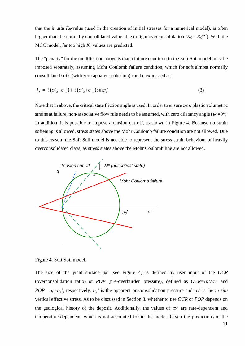
The “penalty” for the modification above is that a failure condition in the Soft Soil model must be
imposed separately, assuming Mohr Coulomb failure condition, which for soft almost normally
consolidated soils (with zero apparent cohesion) can be expressed as:
'sin)''()''( 1321
1321
cff ϕσσσσ ++−= (3)
Note that in above, the critical state friction angle is used. In order to ensure zero plastic volumetric
strains at failure, non-associative flow rule needs to be assumed, with zero dilatancy angle (ψ’=0°).
In addition, it is possible to impose a tension cut off, as shown in Figure 4. Because no strain
softening is allowed, stress states above the Mohr Coulomb failure condition are not allowed. Due
to this reason, the Soft Soil model is not able to represent the stress-strain behaviour of heavily
overconsolidated clays, as stress states above the Mohr Coulomb line are not allowed.
Figure 4. Soft Soil model.
The size of the yield surface p0’ (see Figure 4) is defined by user input of the OCR
(overconsolidation ratio) or POP (pre-overburden pressure), defined as OCR=σc’/σv’ and
POP= σc’-σv’, respectively. σc’ is the apparent preconsolidation pressure and σv’ is the in situ
vertical effective stress. As to be discussed in Section 3, whether to use OCR or POP depends on
the geological history of the deposit. Additionally, the values of σc’ are rate-dependent and
temperature-dependent, which is not accounted for in the model. Given the predictions of the
1
p’
qM* (not critical state)
p0’
Mohr Coulomb failure
Tension cut-off

12
model are very sensitive to the OCR (or POP) values, one needs to be extra careful in the
interpretation of σc’ values. During plastic straining, the size of the yield surface is increasing as a
function of plastic volumetric strains. Hence, in triaxial shearing at the normally consolidated
range, the yield surface increases with plastic volumetric strain until the Mohr Coulomb failure
conditions is reached. At this state, the size of the cap no longer changes. The size of the yield
surface, p0’ is a state variable in the model, which is updated during the analyses.
In terms of compression relationship, the Soft Soil model uses the modified compression index λ*
and the modified swelling index κ*, defined in semi-log scale (using natural logarithm) by plotting
the volumetric strains versus the natural log of mean effective stress. This results in non-linear
elasticity, in contrast to the liner elasticity assumed in the Mohr Coulomb model. By definition,
the λ* and κ* values relate to drained radial stress paths in the p’-q plane (i.e. stress paths with
constant stress ratio η), and cannot be derived based on results from a drained shearing stage. The
actual values are rather straight-forward to define, as shown in Section 3, and can be linked with
the one-dimensional equivalents, the compression index (Cc) and swelling index (Cs), as
demonstrated in Figure 5 (value of 2.3 approximates ln10). The void ratio e, is strictly speaking
not a model parameter in the Soft Soil model, but an input value for initial void ratio e0 is needed
if one wants to account for the changes in permeability (hydraulic conductivity) k, as a function of
changes in void ratio in consolidation analyses.
The elastic part of the SS model, due to the adaptation of the modified swelling index, results in
stress-dependent bulk modulus K’. To describe the elastic relationship fully, in addition to
modified swelling index κ*, another elastic model parameter is needed, namely the Poisson’s ratio
for unloading/reloading νur’. It should be noted that the value for νur’ is not (and should not) be
the same as used for the Poisson’s ratio, for example in the context of purely elastic model or the
Mohr Coulomb model. The values used in the MC model have to be much larger than the “true”
elastic Poisson’s ratio νur’, because in the MC model deformations are assumed to be purely elastic
until failure. The Poisson’s ratio input to the MC model needs to compensate for this assumption.
The undrained shear strength (cu) resulting from the model can be easily defined both for
compression and extension either analytically or by simulating shearing to failure, as discussed in
Section 3. It is hence not an input parameter, but an emerging property and the user needs to check
that with the model parameters assumed, appropriate cu values are predicted.

13
Figure 5. Definition of modified compression and swelling index.
2.3 Soft Soil Creep model
The Soft Soil Creep model (Vermeer et al. 1998, Vermeer & Neher 1999) is a rate-dependent
further development of the Soft Soil model. Instead of yield surface, the boundary between the
small creep strains and the large creep strains is called Normal Compression Surface (NCS), see
Figure 6. The creep strains are assumed to be irrecoverable. It is assumed (erroneously) that NCS
is the contour of constant volumetric creep. The incremental volumetric creep strain is calculated
as:
β
τµδε
=
p
eqcp p
p''*
with *
**
µκλβ −
= (4)
where µ* is the modified creep index, defined in semi-log space, see Figure 7. Just like the
compression indices, it can be linked the 1D creep index Cα. The reference time τ relates to the
loading rate (or strain rate) used in defining the apparent pre-consolidation pressure (see Leoni et
al. 2008 for details). In the Soft Soil Creep model, it has been implicitly assumed that the reference
time τ equals to 1 day, and hence the OCR or POP values used as input must be derived based on
standard 24 h (=1 day) incrementally loaded (IL) oedometer tests. Based on the value for p’p is
calculated within the program. The predictions by the model are super-sensitive for the OCR (or
POP) values.
a) Definition of λ* and κ*
p’ (ln –scale)
εp κ*
λ*
b) Linking of λ* and κ* to Cc and Cs
σv’ (log10 –scale )
e
Cc
Cs
)1(3.2*
eCc
+=λ
eCs
+≈
1*κ

14
The size of NCS to the current stress surface (CSS), i.e. the ratio of p’eq/p’p, in Eq. (3), is a triaxial
equivalent of the inverse of OCR (vertical overconsolidation ratio). The model, therefore, predicts
creep strains both in the normally consolidated and the overconsolidated region. The consequence
of the formulation in Eq. (4) is that if the creep rate when the soil is normally consolidated is a, as
indicated in Figure 6, it is significantly smaller in overconsolidated state, given the exponent β
has typically a rather large value. Similarly to the Soft Soil model, the stress states above the Mohr
Coulomb failure condition (noted with MMC in Figure 6) are not allowed, and hence the model is
not suitable for highly overconsolidated clays.
Figure 6. Soft Soil Creep model.
Figure 7. Definition of the modified creep index.
pp′
q
p´
ce = a
eq pNCS: p p′ ′=
ce a <<
eqp′
CSS
acv =ε
acv <<ε
MCM *M
a) Definition of µ*
t (ln –scale)
εp
µ*
b) Linking of µ* to Cα
t (log10 –scale )
e Cα
)1(3.2*
eCα
+=µ

15
The assumption that the NCS is the contour of constant volumetric creep strains is inappropriate,
as pointed out by Grimstad et al. (2010). The consequence is that excessive creep strains can be
triggered just by the in situ stresses (even outside the loaded area), as shown by Karstunen et al.
(2013). Because of this flaw, the model is not particularly suitable for predicting creep strains in
the typical Scandinavian clays. By artificially increasing the input value for OCR, to scale down
the background creep deformations to correspond to those in situ, is possible in areas where
historic creep records exist, such as some areas in the Central Gothenburg. However, even though
the predicted volumetric creep rates can thus be reduced significantly, the deviatoric creep rates
are still going to be overpredicted by the model. So, adjusting OCR can only be done if there is no
significant shearing, given the value will also affect the emerging undrained shear strength. Hence,
the recommendation of this report is not to use the Soft Soil Creep model, if better alternatives are
available.
2.4 Hardening Soil model
The Hardening Soil (HS) model (Schanz 1998, Schanz et al. 1999) is a rather complex constitutive
model that was developed to overcome some of the limitations of the Soft Soil model, with regards
of the overconsolidated region. The HS model consist of several parts (see Figure 8):
1) A volumetric cap yield surface (which notably has not the same shape as the Soft Soil
model).
2) A shear hardening cone that is “opening” as a function of plastic shear strains.
3) A separate failure yield surface, expressed with Mohr Coulomb failure condition.
Just like in the Soft Soil model, the initial size of the cap surface is defined with OCR (or POP).
The initial size of the shear hardening cone is based on K0NC (coefficient of lateral earth pressure
at rest for normally consolidated state). The default value for the latter is Jaky’s K0NC= 1-sin ϕc’,
which is used in calculating parameter α in Figure 8 within the program. The cap surface is
expanding as a function of plastic volumetric strains, and the flow rule is assumed to be associated
on the cap surface. In contrast, on the shear hardening (cone) yield surface, and on the failure
surface (MC failure), the flow is assumed to be non-associated, and consequently, the ultimate
dilatancy angle ψ’ is an input. Just like in the Soft Soil model, zero dilatancy needs to be assumed
for soft clays.

16
Figure 8. Yield surfaces of the Hardening Soil Model.
The stiffness parameters of the Hardening Soil model are stress-dependent reference stiffnesses,
and hence not model constants. As it is often assumed that the reference pressure pref = 100 kPa,
the default value in Plaxis, the input values refer in practice to unrealistically high stress levels in
comparison to the in situ stress state. The user is however free to choose an appropriate stress level.
The stiffnesses are calculated based on Ohde-Janbu –type of non-linear relationship from the
drained reference stiffness Eiref:
m
ref
irefii ap
aEE
++
='' σ
(5)
where a=c’ cot (ϕ’). For soft clays, the apparent effective cohesion c’ is usually assumed to be
zero and the modulus exponent m=1, which results in semi-logarithmic stress-strain relationship,
similarly to the Soft Soil model.
With the assumptions above, the elasto-plastic stiffnesses under (drained) triaxial shearing are
represented by secant modulus E50’ and the elastic unload-reload modulus by E’ur, which are
defined at given cell pressure σ3’ (see Figure 9). It should be noted that in defining E’50 in Figure
9, shearing is assumed to start from the isotropic axis, which is of course not advisable for natural
soils, if the purpose of the triaxial test is to define the stiffness and the ultimate strength that
correspond to the in situ stress state. Rf is an input value that controls the deviator stress level at
which Mohr Coulomb failure condition is triggered. A typical default assumption is Rf = 0.9, and
given it is a purely numerical parameter, it does not make sense to change it.
α p’p
p’p
q
p’
E50shear hardening
E50 & Eoedcombined hardening
Eoedcap hardening
ηK0

17
Figure 9. Definition of moduli for HS model.
The stress-dependent values of E’50 and E’ur can be calculated based on the input reference values,
for the case with c’=0 kPa and m=1:
=
ref
ref
pEE '' 3
5050σ (6)
=
ref
refurur p
EE '' 3σ (7)
where refE50 and refurE are the reference values of E’50 and E’ur (corresponding to reference pressure
σ3’ = pref), and σ3’ is the cell pressure. In Sweden, the cell pressure is typically selected to
correspond to the in situ horizontal effective stress. Additionally, for the elastic part of the model
an unload-reload Poisson’s ratio νur’ needs to be defined, identically to the Soft Soil model.
In addition to the moduli above, a tangential oedometer modulus is required, which needs to be
defined at the normally consolidated range (see Figure 9) as:
=
ref
refoedoed p
EE '' 1σ (8)
where refoedE is the reference value of the confined modulus E’oed, corresponding to reference
pressure σ1’ = pref. Importantly, σ’1 is the major principal effective stress that is equal to the vertical
effective stress in the oedometer test. Typically, if E’oed is taken to correspond the steepest section
of the oedometer curve (compression modulus ML in Sweden, shown in red), σ’1 is selected to be
equal to the preconsolidation pressure.
εv
σ1σc σ1=pref
Eoedref
1
E50ref
Eurref
qult
q
ε1
qf=Rf qult
σ3=pref
0.5 qf
Triaxial test Oedometer test
’’
’
’ ’
’

18
As discussed further in Section 3, there are difficulties in defining the stiffness parameters for the
HS model based on typical Swedish laboratory testing programme, which does not contain drained
triaxial testing. Furthermore, because the reference moduli correspond to an arbitrary stress level,
defined by pref, it is difficult to have genuine “feel” for typical values. Additionally, in the
implementation of HS model to Plaxis, there are some internal restrictions for the ratios of the
reference moduli, preventing such input of values that would be typically measured for Swedish
clays. Therefore, it is recommended that Soft Soil model is used instead of Hardening Soil model,
unless it is necessary for the geotechnical problem concerned (see Section 2.6). In this report, HS
model is used in all the problems analysed to highlight its limitations in the application to soft
soils.
As illustrated in Figure 8, with the Hardening Soil model, the modulus which is the most important
for the analyses depends on the stress path. The idea of constitutive modelling is to use the same
set of model constants regardless of the stress path. However, with models such as the Hardening
Soil model, which do not allow the user to input the “as measured” reference moduli ratios for soft
soils, it may be necessary to use different values in different zones, as discussed in Section 2.6,
undermining the whole concept of constitutive modelling. There is also an extension of the HS
model that accounts for small strain stiffness degradation, developed by Benz (2007), but that
model is beyond the scope of this report.
2.5 Creep-SCLAY1S model
Creep-SCLAY1 model (Karstunen et al. 2013, Sivasithamparam et al. 2013, 2015), is an
anisotropic creep model for soft clays developed in collaboration between Chalmers, Norwegian
Geotechnical Institute and Plaxis bv. The model has been further extended following the ideas by
Karstunen et al. (2005) to be applicable for sensitive natural clays. This version is in the following
referred to as the Creep-SCLAY1S model. The model is a hierarchical creep model, in which
similarly to its elastoplastic equivalent S-CLAY1S (Koskinen et al. 2002, Karstunen et al. 2005)
features such as evolution of anisotropy and the effect of bonding and destructuration can be
“switched off” by appropriate choice of input parameters. Associated flow rule is assumed, in
contrast to the MAC-S model by Olsson (2013), to keep the model as simple as possible and
numerically stable. The same concepts, such as Normal Compression Surface etc., that are used in
the Soft Soil Creep model are adopted.
The Normal Compression Surface of the Creep-SCLAY1S model is assumed to be initially
anisotropic, similarly to the S-CLAY1 model (Wheeler et al. 2003). The expression was

19
independently proposed by Dafalias (1986), based on thermodynamic considerations, and
Korhonen et al. (1987) based on experimental evidence. When looking at the model in the
simplified case of triaxial space (Figure 10), the equation for NCS can be expressed as:
( ) ( )[ ] 0''')(' 222 =−−−−= pppMpqf pNCS αθ (9)
where α is a state variable (a scalar only in this special case) related to the inclination of the yield
surface, and M is the stress ratio at critical state. M is assumed dependent on Lode angle θ,
enabling to account for the differences of Mc (critical state stress ratio in triaxial compression) and
Me (critical state stress ratio in triaxial extension) measured for soft soils (see Sivasithamparam et
al. (2015) for details). In a case with no measurements of Me, the value can be estimated based on
the friction angle at critical state corresponding to the Mohr Coulomb failure as:
e
ec M
M−
=63'sinϕ (10)
This will though underestimate the Me value. To account for soil sensitivity, and the resulting
additional resistance to yielding, an imaginary Intrinsic Compression Surface (ICS) is introduced
following the ideas of Gens and Nova (1993). The two surfaces are related as follows:
ip pp ')1(' χ+= (11)
where χ is related to the sensitivity St (χ=St-1). It is assumed that the size of ICS is increasing as
a function of the incremental volumetric creep strains:
**'
'κλ
δεδ
−=
i
cpi
i
pp (12)
where λi* is the modified intrinsic compression index, defined identically to the modified
compression index λ *, but based on an oedometer test on reconstituted clay or an oedometer test
on natural clay at such a high strain level that all effects of any apparent bonding have been
destroyed (see Section 3).

20
Figure 10. Creep S-CLAY1S model (after Gras et al., 2017a).
Simultaneously, as the size of ICS is increasing according to Eq. (11) due to irrecoverable creep
strains, the apparent bonds in the clay, represented by state variable χ, are degrading according to
the following degradation law:
( )
+−= cq
cp ba δεδεχδχ (13)
where a and b are the model constants related to bond degradation.
The creep strains are calculated using the concept of viscoplastic multiplier Λ , proposed by
Grimstad et al. (2010), which in the case of Creep-SCLAY1S results in the following expression
for creep strains:
∂∂
Λ='σ
δε NCSc f with
−−
=Λ 2
02
20
2*
''
Kc
Kc
p
eqi
MM
pp
ηα
τµ
β
and *
**
i
i
µκλβ −
= (14)
where η is the stress ratio (η=q/p’) and the rate related parameters µi*, τ and β are the same as in
the Soft Soil Creep model, with the exception that the subscript i in the creep index µi*, again
refers to the intrinsic value. Subscript K0 refers to normally consolidated K0 state.
State variable α (see Figure 10) is used to represent, and track, the evolution of the surfaces as
function of creep strains rates, representing changes in anisotropy. As discussed in Wheeler et al.

21
(2003) and Sivasithamparam et al. (2015), when generalising the model for solving problems with
principal stress rotation in 2D and 3D, a tensor that can be defined analogously to deviator stress
tensor, called deviatoric fabric tensor, needs to be used instead of scalar α. In the simplified case
of triaxial tests on samples cut from the soil in vertical direction, however, the following
simplification can be made for the rotational hardening law, expressing it in terms of the scalar α :
−+⟩⟨−= c
qdcp δεαηωδεαηωδα )
3()
43( (15)
where ω and ωd are model constants related to the evolution of anisotropy. As further discussed
in Section 3, the value for ωd is unique, and therefore can, similarly to the initial value of α, be
theoretically derived based on the assumed value K0nc for soils that are either normally
consolidated or lightly overconsolidated (Wheeler at al. 2003). The McCauley brackets ⟩⟨ are
simply used to keep the predictions qualitatively sensible on the left of critical state line. The
modulus sign | | is needed around the deviatoric creep rate simply due to the common sign
convention in triaxial testing, and disappears in the generalised form of the model.
From the outset, the Creep-SCLAY1S model has significantly more input parameters than the e.g.
the Soft Soil model. Indeed, typically adding any new feature (creep, anisotropy, bonding etc.)
results in additional state variables, which need to be tracked throughout the analyses, and
furthermore, additional model constants that need to be defined. However, as shown in Section 3,
the values for many of the new model constants can be defined in a straight-forward manner,
leaving only 3 model constants (ω, a and b) that need calibration or optimisation. Furthermore,
even those have certain theoretical upper and lower bounds (detailed in Gras et al. (2017a), which
eases parameter optimisation.
2.6 Advantages and disadvantages of the models above
To select the best constitutive model for a particular problem, one needs to first understand the
advantages and limitations of the models, to select a model that is most appropriate to the problem
in question. Second, one must understand the main features of the model chosen, as well as how
the value for the model parameter are derived (see Section 3). Finally, one must appreciate the
sensitivity of the model to various model parameters, both when modelling at single element level
(e.g. modelling triaxial tests with the Lab Test tool in Plaxis) and at boundary value level.

22
In contrast to the Mohr Coulomb model, the Soft Soil model and the Hardening Soil model, as
well as the creep models discussed above, allow for changes in stiffness (non-linear stiffness), and
different stiffnesses for loading and unloading-reloading (Figure 11). There is therefore no reason
for using Mohr Coulomb model for deformation analyses. Furthermore, because the effective
stress paths predicted by the Mohr Coulomb model for undrained loading go straight up in the p’-
q –space, the undrained shear strength can be seriously overpredicted by the MC model in effective
stress based stability analyses for normally consolidated clays (see Figure 12). Therefore, for any
effective stress based undrained analyses and consolidation analyses, it is essential to adopt one of
the hardening models.
Figure 11. Comparison of stiffnesses in the models (after Obrzud 2010): a) Mohr Coulomb model; b) Strain hardening model (e.g. Soft Soil, Hardening Soil); c) Strain hardening model with small strain stiffness (e.g. HS small model).
Figure 12. Undrained shear strength predicted by Mohr Coulomb model for normally consolidated clay vs. typical experimental results.
u
uf
ESPTSP
q
p’
2cu
2cu from MC

23
If long-term creep deformations are not of interest, the user can opt for either the Soft Soil Model
or the Hardening Soil model in Plaxis. For soft soils, when m = 1 is adopted for the modulus
exponent in the HS model, both models result in a semi-logarithmic stress-strain relationship, even
though the input parameter are totally different. As demonstrated in Section 3, it is much easier
to derive the values of the model parameters for the Soft Soil model than the Hardening Soil model.
Given the user defines in the Soft Soil model and the HS model what K0NC value that they would
like the models to predict, even though the yield surfaces are different, the differences in
predictions for many stress path are rather minor. Hence, it is in theory possible to use either of
the models e.g. for loading problems. However, for K0 consolidation or groundwater lowering (see
Figure 13), there is no real benefit in using the Hardening Soil model. It needs more input
parameters and furthermore, as shown in Section 3, typical Swedish laboratory testing programme
does not have the tests needed for direct parameter derivation. Additionally, the implementation
of the HS model in Plaxis does not allow to enter the parameter combinations for stiffness that
would typically represent Swedish soft soils. Therefore, for typical loading problems, it would be
advisable to adopt Soft Soil model instead of the HS model.
In contrast, for any shearing that results in stress paths that are steeper than the K0 consolidation
line, the elasto-plastic deviatoric hardening mechanism in the Hardening Soil model would be
triggered (see Figure 13), in addition to the (isotropic) volumetric hardening, resulting in
differences in the two model predictions. When looking at unloading problems, almost identical
elastic heave will be predicted for any soil elements at the bottom of the excavation by the Soft
Soil and HS models, if m=1 is assumed in the latter. For infiltration and active wall problems,
however, the Soft Soil model would forecast purely elastic unloading, whilst with the Hardening
Soil model, elasto-plastic deformations are triggered. Given all combination of moduli are not
possible in the HS model, the dilemma is then to decide which modulus is most important. Some
indication for that is given in Figure 14, considering different areas in a typical anchored retaining
structure. At far field, much higher values of stiffness, corresponding to the small strain stiffness
E0’ (see Figure 11) is required. You may also choose to assume E0’ behind the wall in case of
excavation as a cantilever when placing an anchor and pre-stressing that, given this results in a full
stress path reversal.
As pointed out by Janbu (1977), for earth retaining structures on soft soils, the most critical
condition in terms of stability is the drained situation. As both Soft Soil Model and Hardening Soil
model assume Mohr Coulomb failure condition (constant friction angle), they tend to be overly
conservative in triaxial extension. Hence, for deep excavations in soft soils, failure due to bottom

24
heave can be predicted too early with these models. This aspect can be improved by adopting a
model that allows for the direct input for the stress ratios at critical state for both compression and
extension, as is possible with the Creep-SCLAY1S model.
Figure 13. Examples of loading and unloading problems as modelled with Hardening Soil model (after Obrzud 2010).
There are, however, situations, when adopting a rate-dependent model is beneficial and necessary.
For example, if an earth retaining structure appears to be stable in undrained condition, and yet
fails in drained conditions, a question arises: how long can the excavation be kept open? It is not
only consolidation, but creep that needs to be considered. Furthermore, when constructing in urban
areas, it is important to predict displacements both in the short-term (construction time) and in the
long term (life time of the structure). For these type of situations, as well as foundations and
embankment on soft soils, it would be advisable to opt for a creep model. A summary of the
discussion above in presented in Table 1.
(MC)
p p
p p

25
Table 1. Key features of the constitutive models considered.
Constitutive model
Model feature Mohr
Coulomb
Soft Soil
Soft Soil
Creep
Hardening
Soil
Creep-
SCLAY1S
Non-linear stiffness x * x x x x
Stress-dependent
stiffness x x x x
Different stiffness for
loading/unloading x x x x
Associated flow x Cap x Cap x
Non-associated flow x MC x Cone, MC
Stress history effect x x x x
Volumetric hardening x x x x
Deviatoric hardening x x
Anisotropy x**
Bonding and
destructuration x
Rate-dependency x x *Only bi-linear MC– Mohr Coulomb failure surface Cap – Cap yield surface in SS and HS Cone – Deviatoric hardening conical yield surface in HS ** Only for large strains
As discussed in Section 3, the laboratory testing needs to be planned accordingly. Creep models
are super-sensitive to the values of the apparent preconsolidation pressure (input via OCR or POP),
and furthermore, the values of the apparent preconsolidation pressure are severely rate-dependent.
For simple hand calculations, it is possible to use CRS test results in deriving the values for
apparent preconsolidation pressure, at least for clays that are known to exhibit same creep rates,
so that appropriate correction for rate-effects can be made. However, as discussed by Muir Wood
(2016), the strain-rate effects in CRS tests are not solely due to creep effects. In particular for a
case when more complex non-linear constitutive models are used, including the models discussed
in the report, the correction of the apparent preconsolidation pressure from CRS to correspond to
that in 24-h IL test is not trivial. The results from CRS tests would namely need to be interpreted
at system level.

26
In Section 3, the determination of model parameters is addressed using data from Utby test site in
Gothenburg. Firstly, common parameters, such as apparent preconsolidation pressure, Poisson’s
ratio and strength parameter are discussed, followed by model by model description of the
determination of stiffness parameters.
Figure 14. Importance of various moduli in a case of anchored retaining wall (source unknown).

27
3 Determination of model parameters
3.1 Common model parameters
3.1.1 Apparent preconsolidation pressure σ’c The apparent preconsolidation pressure σ’c is a key state variable for all the advanced models
considered, and during the analyses the value is changing. The predictions by the Soft Soil model
and the HS model are very sensitive for the values of OCR or POP, and the creep models are super-
sensitive for selected the values. Hence, OCR or POP are one of the most important input values.
The sensitivity of the solution to the input value of σ’c should be checked at boundary value level.
The value for apparent preconsolidation pressure σ’c depends on the sedimentation history as well
as post-depositional history, aging and cementation. The post-depositional processes include
natural processes such as further deposition and erosion, as well as the effects of human influence,
such as historic fills and loads from existing structures. In Scandinavia, many of the soft clay
deposits were formed during/after the last ice age, and following deposition and consolidation
under the self-weight have been exposed to secondary compression (see Figure 15b). Furthermore,
especially in a river environment, clay deposits have possibly been exposed to erosion (see Figure
14a), due to meandering and changes is water levels and flow rates. Sensitive clays also bear
evidence on some apparent bonding that exhibits as higher than expected values for the
preconsolidation stress (see Figure 14c), and the in situ void ratio. Hence, most of the clay deposits
in Scandinavia would be expected to be lightly overconsolidated.
The values of the apparent preconsolidation pressure need to be determined in laboratory, by
conducting one-dimensional compression tests on fresh (max. two weeks old) high quality samples
under controlled temperature conditions. The effects of sample disturbance can be easily seen
when plotting the results in semi-log scale (see Figure 16). The “remoulded” line, with no clear
kink would be for example typical for a sample that had been freezing and thawing before testing.
The values of the apparent preconsolidation pressure are also dependent on the strain-rate, i.e. the
higher the strain-rate the higher the preconsolidation pressure. In particular for creep models, this
has serious implications. As discussed in Section 2.3, the apparent σ’c value for the Soft Soil Creep
model needs to correspond the reference time τ assumed in the model to be 1 day. Hence, for the
creep models conventional incremental 24 h step oedometer tests, referred to in the following as
incremental loading (IL) tests, are necessary. In Sweden, often only CRS tests are conducted.

28
Given different clays (in particular clays with very different sensitivities and mineralogy) have
different tendency to creep, it is not possible to have universal methodology for strain-rate
correction of σ’c. Because of that, the so-called Sällfors (1975) method, often used to correct σ’c
from a typical Swedish CRS test to be equivalent to the one from IL, might work reasonably well
for the clays from the locations and depths the method was tested for, but is not universal and
applicable to all. Recent research has highlighted that in the case of non-linear elasto-plastic
models, the interpretation of a CRS test would need to be done at system level (Muir Wood 2016).
Therefore, for advanced creep models, it is necessary to conduct IL oedometer tests.
Figure 15. Effect of a) erosion, c) creep and c) creep and cementation of the apparent preconsolidation pressure.
A standard Swedish CRS tests is, however, very useful in defining the load steps for a step-wise
oedometer test. Figure 17 shows CRS test results for a sample of Utby clay. Because most of the
Sedimentation Erosion

29
constitutive models discussed in this report are based on stiffnesses derived in semi-log scale, the
interpretation has been done in the same scale, using interpolated curves. However, the results
have also been checked in linear scale. The CRS curve in Figure 17a aided the design of load steps
for the IL test shown in Figure 17b. Alternative interpretation methods on the IL results suggest
minimum value of 91 kPa and maximum value of 98 kPa (the latter is derived with Casagande’s
method) for σ’c. One would expect the CRS test to result with much higher σ’c value, given the
strain-rate is higher than in IL tests. However, in this case the uncorrected CRS gives a low-end
estimate. Even though the samples are from the same block, the initial void ratios differ, indicating
either subtle variability or some disturbance in trimming and setting up the samples.
Figure 16. Effect of sample disturbance on the stress strain response and apparent preconsolidation pressure (after Barnes 1995).
Once the value of σ’c has been carefully selected, it is a good practice to plot the values versus
depth (or preferably absolute level) against the most likely distribution of in situ effective vertical
stress, as illustrated in Figure 18. Namely, dependent on the geological history of the deposit, in
the input for the FE code, either constant POP or constant OCR should be used, see Figure 18.
High quality step-wise oedometer testing is also needed for defining the compressibility
parameters for the advanced models, as discussed in the following. Given the elastic parameters
are best derived based on unloading-reloading loops, this again speaks in favour of step-wise
oedometer tests, given in an IL test the load is always known. In CRS test one needs to be extra
careful with the calibration of the load cell, and furthermore, the unloading needs to be done slowly
enough to ensure that the piston is always in contact with the sample.

30
Figure 17. CRS (left) and incremental load (IL) tests on STII tube sample from Utby.
Figure 18. Effect of geological history on the preconsolidation pressure (after Parry & Wroth 1981).
Stress
Dept
h σ’v
σ’c
OCR = const.
OCR
Dept
h
Constant with depth
321
Desiccation
Stress
Dept
h σ’v
POP = const.
σ’c
OCR
Dept
h
Decrease with depth
321
Present
Past lowest
b) Changes in GLW
a) Creep and aging

31
3.1.2 Strength & dilation parameters and K0NC
Even though the standard and advanced models considered in this report may have different input
parameters for describing the soil strength in terms of effective stresses, the interpretation of
experimental data is similar. Figure 19 shows the experimental results on Utby clay in p’-q –space,
which is most convenient way of interpreting the effective strength parameters for the constitutive
models concerned. The tests are undrained triaxial tests where the initial consolidation has been
anisotropic (until the estimated in situ effective stresses), before shearing to failure in compression
and extension, respectively. The failure at critical state in undrained tests is interpreted to
correspond to stable excess pore pressures (not shown). Given the soil is overconsolidated, the
stress path to failure in triaxial compression is largely elastic. Alternatively, results from drained
triaxial tests could be used, see Figure 20. The problem, however, is that for very soft soils the
stress ratio η often just keeps on increasing during shearing, and at the strain level when the test is
stopped, the sample is extremely deformed. The bulging of the sample and any strain localisation
within the sample affects the interpretation of the results, and clearly after 5% strain the results are
no longer reliable. Continuing the test would simply mean that the interpretation would need to be
done at system level, by performing a finite element simulation of the test. Often, the Bishop-
Wesley cells run out of travel well before the critical state when shearing very soft soils. Drained
triaxial tests are, however, necessary for estimating the reference moduli E50ref and Eur
ref for the
Hardening Soil model, as discussed in Section 3.5.
The Hardening Soil model and the Soft Soil model adopt Mohr Coulomb failure condition, which
is Lode angle dependent. The model predicts different strengths in triaxial compression and
extension, assuming the (critical state) friction angle ϕ'c to be constant. As the experimental results
for Utby clay in Figure 19 demonstrate, for Swedish clays in triaxial extension the critical state
friction angle is much higher than in compression. In the Creep-SCLAY1S model, the values for
critical state stress ratio in triaxial compression Mc and triaxial extension Me can be given
separately. Because the Hardening Soil and Soft Soil models assume Mohr Coulomb failure
condition, it is also necessary to input value for the ultimate dilatancy angle ψ’. At critical state
ψ’=0°. In the Creep-SCLAY1S model, zero volume at critical state is inherent to the model.
The friction angle at critical state ϕ'c is used to estimate the input value for K0NC, the coefficient of
lateral earth pressure at rest under normally consolidated condition. This is a direct input in the
Soft Soil, Soft Soil Creep and Hardening Soil models. Unless measurements are made, e.g. with
K0 triaxial cell (Olsson 2013), K0NC can be estimated with Jaky’s formula as K0
NC=1-sin ϕ'c. As
discussed in Section 3.6, Jaky’s formula is also assumed in calculating the state variable associated

32
with initial anisotropy (α0) and one of the model constants related to the evolution of anisotropy
in the Creep-SCLAY1S model.
Figure 19. K0 -consolidated undrained triaxial tests on Utby clay in compression (left) and extension (right).
Figure 20. Drained triaxial test on Utby clay.
3.1.3 Poisson’s ratio for unloading-reloading νur Poisson’s ratio for unloading-reloading νur is a purely elastic input parameter for all models
concerned. For soft soils, most often a constant value of 0.1<νur < 0.2 is assumed. Once all other
model parameters are fixed, it is possible to fine-tune the values by simulating the loading-
unloading loops in a drained triaxial tests. At boundary value level, when modelling soft soil
problems, the model predictions do not tend to be particularly sensitive to the selected value of
Poisson’s ratio. It is, however, advisable to check this by performing a sensitivity study, especially
for problems where the horizontal stresses are important, such as problems involving retaining
structures.

33
3.2 Stiffness parameters of the Soft Soil model
The key model parameters related to the stiffness of the soil in the SS model are the modified
compression index λ* and the modified swelling index κ*. They can be easily derived by plotting
the oedometer results in semi-logarithmic scale. If void ratio e is used rather than the volumetric
strain εp, repeatability of the tests and the soil state for each sample can be assessed. First, we can
define the 1D equivalents, compression index Cc and swelling index Cs, as done in Figure 21.
These can then be easily converted to the modified indices by using the equations in Figure 5. The
value for Cc (and hence λ*) for sensitive clays depends on the stress level. However, in most
geotechnical applications the effective vertical stress after construction is unlikely to exceed the
apparent preconsolidation pressure by hundreds of kPas. Hence, one should typically fit the elasto-
plastic stiffness against the steepest part of the stress-strain curve, as done in Figure 21. For the
swelling index, strictly speaking an unload-reload loop is required, but as such were not available
in these particular tests, the initial slope has been used instead. The values of λ* and κ* from the
CRS results and the IL odometer results in Figure 21 are for practical purposes almost identical,
which is not necessarily always the case.
3.3 Stiffness and creep parameters for the Soft Soil Creep model
The stiffness parameters of the Soft Soil Creep model are identical to the Soft Soil model. The
only additional parameter needed, in addition to the pre-fixed reference time τ that is 1 day, is the
modified creep index µ*. As discussed in Section 2.3, the modified creep index is defined by
plotting the volumetric strain as a function of natural logarithm time for a given stress increment
in IL oedometer test. Results for Utby clay are plotted in Figure 22. It is typical for sensitive clays
that the value depends on the stress level, because µ* is not a totally independent quantity: the
value depends on the compression index, and in particular just at the onset of yielding, the highest
values for µ* are encountered. For input in a creep model, however, one would like to have a value
that presents the “pure creep” of the material, the so-called intrinsic creep µi*. That corresponds
to the values at the highest stress levels, and ideally the final load stage is also left on as long as
possible. Based on the results in Figure 22, µ*=0.0035-0.0040 would seem appropriate. Because
the stage with stress increase to 281 kPa has longer duration that the next stage, a value of
µ*=0.0035 is selected. For a true intrinsic value, tests on reconstituted clay sample from the same
depth would need to be made. The IL test on reconstituted Utby clay yielded a much lower value
µi*=0.0014, which is adopted for the analyses.

34
Figure 21. Determination of the stiffness parameters for the Soft Soil model for Utby clay.
3.4 Stiffness parameters for the HS model
The Hardening Soil model requires values for three reference moduli as input: the reference
(secant) triaxial stiffness refE50 , the unload-reload (secant) stiffness refurE and the reference (tangent)
oedometric stiffness refoedE . These all refer to values at a given reference pressure pref. For the triaxial
moduli refE50 and refurE the reference pressure pref refers to the cell pressure σ’3 used in shearing,
whilst in contrast for the oedometric modulus refoedE the reference pressure pref refers to σ’1, the
effective vertical stress. As oedE (referred to M’ in Sweden) varies significantly as a function of the
effective vertical stress, the value used in the context of the HS model has to be representative of
the expected stress levels in the problem to be analysed at normally consolidated region. In the
following refoedE refers to the value corresponding to σ’1 = pref, which was taken as 100 kPa.
As shown in Figure 9, refoedE needs to be defined in the normally consolidated region. Given it is
important to have an elasto-plastic stiffness that represent correctly the soil stiffness at the relevant
stress range, in most cases it is best to define the value just after the onset of yield (referred to ML
in Swedish practice), just like was done for λ* for the Soft Soil model, see Figure 23. It is rather
unlikely that the ML value would corresponds exactly to the vertical effective stress σ’v of 100 kPa.
Instead, it typically corresponds to a stress level that is around (or marginally higher than) the
apparent preconsolidation pressure σ’c. Please note that in case CRS results are used, the σ’c has
to be corrected for strain-rate effects (i.e. Sällfors (1975) correction, or something similar, has to
be applied first). By substituting ML to E’oed, the (corrected) σ’c for σ’1, and choosing reference

35
pressure pref as 100kPa, it is possible to solve for refoedE in Eq. (8). The value that is now input
corresponds to a rather random stress level: i.e. you input the oedometric stiffness for a given layer,
as if that layer was located at much greater depth. Therefore, one no longer can the same “feel”
for the values input for a given layer, unless a layer-specific pref value is adopted.
Figure 22. Modified creep index µ* for Utby clay.
Figure 23. Definition of M0 and ML.
εv
M
∆εv
∆σ’v
σ’v
σ’v
ML
M0

36
Plaxis manual proposes that:
ref
refoed p
E *λ= (15)
Then, using that formula, the program would calculate the applicable value of oedE based on Eq.
(8), with assumed value of m (m=1). In sensitive clays, the resulting oedometric modulus would
be erroneous, unless both λ* and pref correspond to the maximum rate of yielding. It is possible to
check for the “real” m value, which could be determined by selecting two Eoed - σ’1 –pairs on the
oedometric curve, and substituting them to Eq. (5), to solve for the m –value. Typically for
sensitive clays m >1, which is not allowed as input. Therefore, it is advisable when using Eq. (15)
to assume layer-specific values for pref rather than using an arbitrary default value of 100 kPa
suggested by the program.
The other two moduli refE50 and refurE are drained triaxial moduli, and need to be determined in terms
of effective stresses. For that, a drained triaxial tests with unload-reload loop is ideally needed.
This principle is shown in Figure 24 for Utby clay. Note that the strains are reset after the
anisotropic consolidation stage, given it is the shearing stage that matters. The subscript 50 in refE50
refers to the secant modulus at deviator stress level that is 50% of that in failure. In this case, the
cell pressure during shearing was σ’3 = 32 kPa, and the corresponding E’50 = 5000 kPa. Assuming
reference value pref =100 kPa, based on Eq. (6), the input value is refE50 = 15 625 kPa. In same
manner, using Eq. (7), the value of E’ur for σ’3 = 32 kPa is converted to refurE = 26 978 kPa for the
model input.
Drained triaxial tests, however, are not common in Sweden. In Figure 25, results from undrained
triaxial test on Utby clay have been used to derive the undrained reference value urefE −50 = 29 615
kPa, corresponding to reference pressure pref = 100 kPa. Note that again the strains are reset after
the anisotropic consolidation stage. For an elastic material, it would be easy to convert an
undrained modulus to the drained equivalent using Equation:
)'1(32' ν−= uEE (16)
where E’ is the Young’s modulus in terms effective stresses, Eu is the undrained Young’s modulus
and ν’ is the elastic Poisson’s ratio. However, both urefE −50 and refE50 are elasto-plastic parameters,

37
not elastic parameters. Substituting the undrained reference stiffness from Figure 25 into Equation
(16), assuming ν’=0.2, results in refE50 = 15 794 kPa (same order of magnitude as the reference
stiffness from drained test), suggesting that the values derived are perhaps elastic parameters. The
Plaxis manual lists several possible options for “converting” the moduli, but the ratio of refurE / refE50
is by no means a constant for soft soils. Just like the Cs/Cc or κ*/λ* ratio, it depends on the level
of plastic strain mobilisation and on the sensitivity of the soil, as well as the sample quality.
It is possible to use the unload-reload loop (or initial elastic slope M0) in oedometer test to estimate
the triaxial unload-reload modulus 'urE :
)1()1)(21(
)1)(21()1( 0
0 vvvME
vvEvM ur
ur
′−′+′−
=′⇔′+′−
′′−= (16)
which corresponds to σ’3= K0NCσ’c. The value can be substituted to Eq. (7) to solve ref
urE
corresponding to the reference pressure pref = 100 kPa.
Figure 24. Determination of refE50 and refurE for Utby clay based on drained triaxial test.
The discussion above demonstrated that the parameters for the HS model are significantly trickier
to derive than the ones for the Soft Soil model. If only undrained triaxial tests are available, the
Lab Test tool in Plaxis may need to be used to adjust the parameter values, to ensure that the test
results available (oedometer and undrained triaxial test) can be simulated reasonably well, before
commencing with FE analyses. Hence, instead of deriving model parameters, the model
parameters for the HS model must be always calibrated by model simulations. A major problem
is that in the implementation of Hardening Soil model in Plaxis, some limits for the ratios of moduli
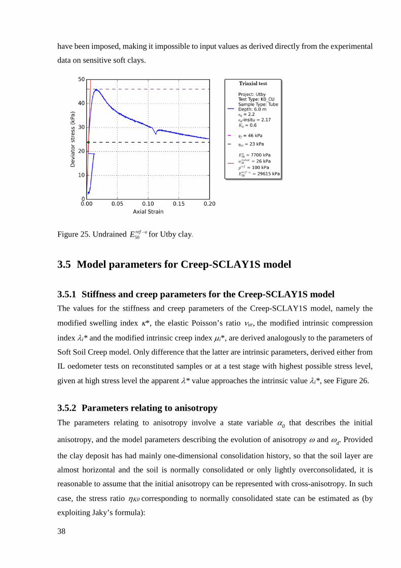
38
have been imposed, making it impossible to input values as derived directly from the experimental
data on sensitive soft clays.
Figure 25. Undrained urefE −50 for Utby clay.
3.5 Model parameters for Creep-SCLAY1S model
3.5.1 Stiffness and creep parameters for the Creep-SCLAY1S model The values for the stiffness and creep parameters of the Creep-SCLAY1S model, namely the
modified swelling index κ*, the elastic Poisson’s ratio νur, the modified intrinsic compression
index λi* and the modified intrinsic creep index µi*, are derived analogously to the parameters of
Soft Soil Creep model. Only difference that the latter are intrinsic parameters, derived either from
IL oedometer tests on reconstituted samples or at a test stage with highest possible stress level,
given at high stress level the apparent λ* value approaches the intrinsic value λi*, see Figure 26.
3.5.2 Parameters relating to anisotropy The parameters relating to anisotropy involve a state variable α0 that describes the initial
anisotropy, and the model parameters describing the evolution of anisotropy ω and ωd. Provided
the clay deposit has had mainly one-dimensional consolidation history, so that the soil layer are
almost horizontal and the soil is normally consolidated or only lightly overconsolidated, it is
reasonable to assume that the initial anisotropy can be represented with cross-anisotropy. In such
case, the stress ratio ηΚ0 corresponding to normally consolidated state can be estimated as (by
exploiting Jaky’s formula):

39
c
cK M
M−
=63
0η (17)
where Mc is the critical state stress ratio in triaxial compression.
In the special case above, there is only one α -value that would predict no lateral irrecoverable
strains. When associated flow is assumed for the normal compression surface defined by Eq. (9),
αK0 can be solved as (see Wheeler et al. (2003) for details):
2 20
0 0 3c K
K KM ηα η −
= − (18)
Similarly, the value for the model constant ωd can be determined from Μc as proposed by Wheeler
et al. (2003), thus ωd is not an independent soil constant.
( )( )
2 20 0
2 20 0
3 4 4 3
8 2c K K
dK K c
M
M
η ηω
η η
− −=
+ − (19)
Figure 26. Compressibility and destructuration of natural clay vs. reconstituted clay.
ε p Reconstitutedsoil
Naturalsoil
1
1
ln p’
λ∗
λi∗
χ0 p’i p’cp’i

40
Finally, following the logic presented in Leoni et al. (2008) an initial value for ω can be estimated
as:
++
−≈
dKc
dKc
i MM
ωαωα
κλω
02
02
2210
ln*)*(
1 (20)
The ω value derived can be further calibrated by comparing model simulations of an triaxial test
that is sheared to failure in extension, following an anisotropic consolidation to in situ stress level,
against experimental data.
3.5.3 Parameters relating to bonding and destructuration The initial value for the state parameter that defines the amount of bonding χ0 can be estimated by
the sensitivity St of the soil as:
10 −= tSχ (21)
which is typically measured via fall cone test on natural and remoulded samples. In highly sensitive
clays and quick clays the latter may not be possible, and in such cases the value can be estimated
by comparing the stress-strain curves of the natural and reconstituted samples (at a given void
ratio), as indicated in Figure 26. By definition χ0 is always ≥ 0.
As discussed by Koskinen et al. (2002), the determination of destructuration parameters a and b
require optimisation. One method is to perform a drained isotropic (or pseudo-isotropic triaxial
test) and simulate that with an assumed ‘sensible’ value of b, given a stress path which produces
mainly volumetric strains, is insensitive to b value. Subsequently, a drained test with high stress
ratio could be performed, to optimise the value for b. Theoretically, the bounds for b are 0 < b <
1. Experience so far with Scandinavian and Scottish clays suggests b values 0.2 < b < 0.4. The
predictions are much more sensitive to a value than b value, which is also apparent from Eq. (13).
Gras et al. (2017a) propose some theoretical upper and lower bounds for a dependent on
irreversible compressibility, defined as λi∗-κ∗:
( )
+−
+≤
20
0
0
21**
)1(
c
Ki
Mb
aα
κλχ
χ (22)

41
( )**)1()2
1ln()22ln(
2ln0
0 κλχ
χ −+
+−+
≥
iba (23)
With typical values of λi∗-κ∗, the a values are typically around 8-12.
3.5.4 Parameters relating to rate-dependency and creep The creep parameters of the Creep-SCLAY1S model, namely reference time τ and the modified
intrinsic creep index µi* are identical of those of the Soft Soil Creep model. The value for the
reference time is dependent on the loading rate used in the incrementally loaded oedometer test
used for defining the value for the apparent preconsolidation pressure. Most importantly, the value
of the modified creep index is the intrinsic value, associated with ‘pure’ creep once all the bonds
are destroyed. It hence refers to the value for a reconstituted sample, or the value at such a high
stress level that there is no bonding left.
3.5.5 Exploiting the hierarchy of the model in parameter choice
Creep-SCLAY1S model is a hierarchical model, and hence by the choice of values for various
material parameters, it is possible to switch off some model features, if these are deemed to be
unimportant or there is not suitable experimental data. Both the effect of bonding and
destructuration, as well as anisotropy can be ignored by suitable parameter choice. In contrast, it
is not possible to switch off rate-dependency and creep. If that is required, it is best to revert to the
rate-independent S-CLAY1S model (see Karstunen et al. 2005).
Firstly, it is possible to switch off bonding and destructuration by assuming χ0 = 0. In order to still
predict the volumetric stiffness correctly, instead of the intrinsic value of λi∗, the corresponding
value for the natural soil λ∗, equal to that in Soft Soil and Soft Soil Creep model need to be
selected.
Secondly, it is possible to switch off anisotropy. For example, if one wanted to simulate a triaxial
tests where the sample has been consolidated isotropically well beyond the yield stress, as would
be conventionally done for deriving the effective strength parameters based on Mohr’s circles, one
would need to switch off the initial anisotropy at the start of the simulations of the shearing stage
by setting α0 = 0. This alone would not switch off the evolution of anisotropy. In order to switch
42
off the evolution of anisotropy, additionally ω = 0 need to be assumed. In the case just discussed,
this would not be advisable, given anisotropy will develop during shearing.
If both bonding and anisotropy are totally switched off, the model becomes a rate-dependent
version of the isotropic Modified Cam Clay (MCC) model, with the associated poor K0 prediction.
To avoid that, it would be better to still account for initial anisotropy by assuming α0 = αΚ0 ,
combined with no evolution of anisotropy by assuming ω = 0. This would also ensure that the
emerging undrained strength in compression and extension would be qualitatively much better
predicted than by the isotropic models.
3.6 Soil tests for determination of model parameters for soft clays
The standard and advanced models discussed above have all one key thing in common: the results
depend on the value assumed for the apparent preconsolidation pressure. In particular, the creep
models are super-sensitive to the value assumed. Given preconsolidation pressure is both rate- and
temperature-dependent, the values are best determined from incrementally loaded (IL) oedometer
tests done at a representative temperature level. The same test would also provide the necessary
information required for the stiffness and creep parameters. However, the ability to capture
accurately the apparent preconsolidation pressure in an IL test depends on the sizes of load
increments used and their magnitude relatively to the in situ vertical effective stress. Therefore,
the IL tests are best planned with an initial CRS test used in informing on the planning of
appropriate load increments.
A CRS test in principle enables also to have an independent assessment of the modified
compression index λ∗, as needed for the Soft Soil and Soft Soil Creep models. However, normally
the stress levels are not such that any estimates of the intrinsic values λi∗ could be made for the
Creep-SCLAY1S model. Furthermore, the initial (elastic) slope in a CRS test is significantly
affected by tendency of the sample to swell, and at the early stages of the test the effective stresses
are unknown. Given the load is continuously ramped via imposing a constant displacement, the
strain-rates vary during the test, the pore pressures in the sample will not always be in equilibrium,
and consequently the results of a CRS tests would, need to be interpreted as a boundary value
problem (see Muir Wood 2016).
The shear strength parameters, i.e. the friction angle at critical state, or alternatively the stress ratio
at critical state, require consolidated undrained triaxial tests, as without it is difficult to estimate
the ultimate strength and the value for normally consolidated K0, affecting the predicted strain

43
paths. For unloading and excavation problems these should ideally include also a triaxial test with
shearing in extension. The latter would also ease calibrating the model parameter ω related to the
evolution of anisotropy. Given the strain predictions in many of the advanced models depend on
the value of stress ratio at critical state, it is not advisable to use empirical values, such as assuming
friction angle to be 30°, as commonly done in Sweden. The stiffness parameters for the Hardening
Soil model, ideally require the results of a drained triaxial test, ideally with an unloading/reloading
loop. Indeed, for any excavation and unloading problems, it would be highly advisable to perform
some drained unload-reload loops at representative stress levels regardless of the model. Finally,
when it is known that advanced FE analyses will be conducted, it is advisable that the laboratory
testing programme has some redundancy, so that there are, in addition to the type of tests that are
needed for the determination of the model parameters, additional tests that can be used for
independent validation of the model and the parameters selected.
With only CRS results, as common in Sweden, preliminary analyses can be done, provided there
is some local knowledge of the friction angle at critical state, combined with sensitivity studies
that look at the influence of OCR on the predictions.
Table 2. Necessary (N) and recommended (R) laboratory testing for the constitutive models
considered.
Constitutive model
Laboratory test Mohr
Coulomb
Soft Soil
&
MCC
Soft Soil
Creep
Hardening
Soil
Creep-
SCLAY1S
Sensitivity (fall cone) N
CRS N N N N N
IL R N R N
IL rec* R
CAUC N N N N N
CAUE** R/N R/N R/N N
CADC with
unload/reload loops*** R R R/N R
* IL on a reconstituted sample ** CAUE needed for unloading/excavation problems & slope stability problems *** CADC with unload/reload loops recommended for unloading/reloading problems with all models

44
4 Validation of model parameters for Utby clay
4.1 Model parameters for Utby clay
Following the procedures above, values for the model parameters for Utby clay have been
determined based on experimental results on SPII samples from a clay layer at 6-8 m depth. For
all models, parameters related to the initial stress state need also to be defined, as listed in Table
3. Given parameters, such as OCR and K0nc are important for all models, the values have been
repeated in the subsequent tables when needed for input, to emphasize that the value is the same
regardless of the model. When simulating experiments, however, the input values for OCR/POP
must be changed to correspond to the conditions in the specific test, as testing rarely starts with in
situ stresses. In particular, the latter is true for oedometer testing where testing starts at much lower
effective stress level than the in situ effective stress.
Tables 4-7 list the parameters derived for the Soft Soil & Soft Soil Creep models, the isotropic
Modified Cam Clay model (MCC), the Hardening Soil model and the Creep-SCLAY1S model.
For Hardening Soil model, two sets of model parameters are included: Set 1 corresponds to the
values when the stiffness is derived based on drained triaxial test results, and Set 2 corresponds to
oedometric conditions. For sensitive clays, given m>1 is not possible, and there are limitations to
the stiffness ratios, this results in two extremely different sets values. In particular, the low
oedometric stiffness results in a super-low value for refE50 . The values for the Hardening Soil model
parameters in Set 1 have been derived based on the drained triaxial test results, to avoid any issues
with strain-rate effects in pore pressure development in an undrained test.
Table 3. Utby clay: common initial stress state parameters.
Initial stress state parameters
Description Symbol Value
Initial void ratio e0 2.05
Bulk density [tons/m3] ρ 1.58
Hydraulic conductivity [m/day] k 8e-5
Coefficient of later earth pressure in situ K0 0.6
Overconsolidation ratio in situ OCR 1.45

45
Table 4. Utby clay: model parameters for Soft Soil & Soft Soil Creep model.
Soft Soil & Soft Soil Creep model
κ* ν ur λ* ϕ'cv [°] ψ [°] K0nc µ* OCR
0.020 0.2 0.296 38.3 0 0.38 0.00142 1.45
Table 5. Utby clay: model parameters for Modified Cam Clay model.
Modified Cam Clay model
κ ν ur λ e0 Μ OCR
0.061 0.2 0.903 2.05 1.56 1.45
Table 6. Utby clay: model parameters for Hardening Soil model.
Hardening Soil model
Symbol Definition Set 1 Set 2 refurE [kPa] Unloading/reloading stiffness 30000 7500
ν ur Poisson’s ratio for unloading/reloading 0.2 0.2 refE50 [kPa] Secant stiffness from drained triaxial 15000 421
refoedE [kPa] Tangent stiffness from oedometer test 4700 337
pref Reference stress for stiffness 100 100
m Power of stress-level dependency 1 1
ϕ'cv [°] Critical state friction angle 38.3 38.3
ψ [°] Dilatancy angle 0 0
K0nc K0 for normally consolidated state 0.38 0.38
OCR Overconsolidation ratio 1.45 1.45
Rf Failure ratio (default value) 0.9 0.9
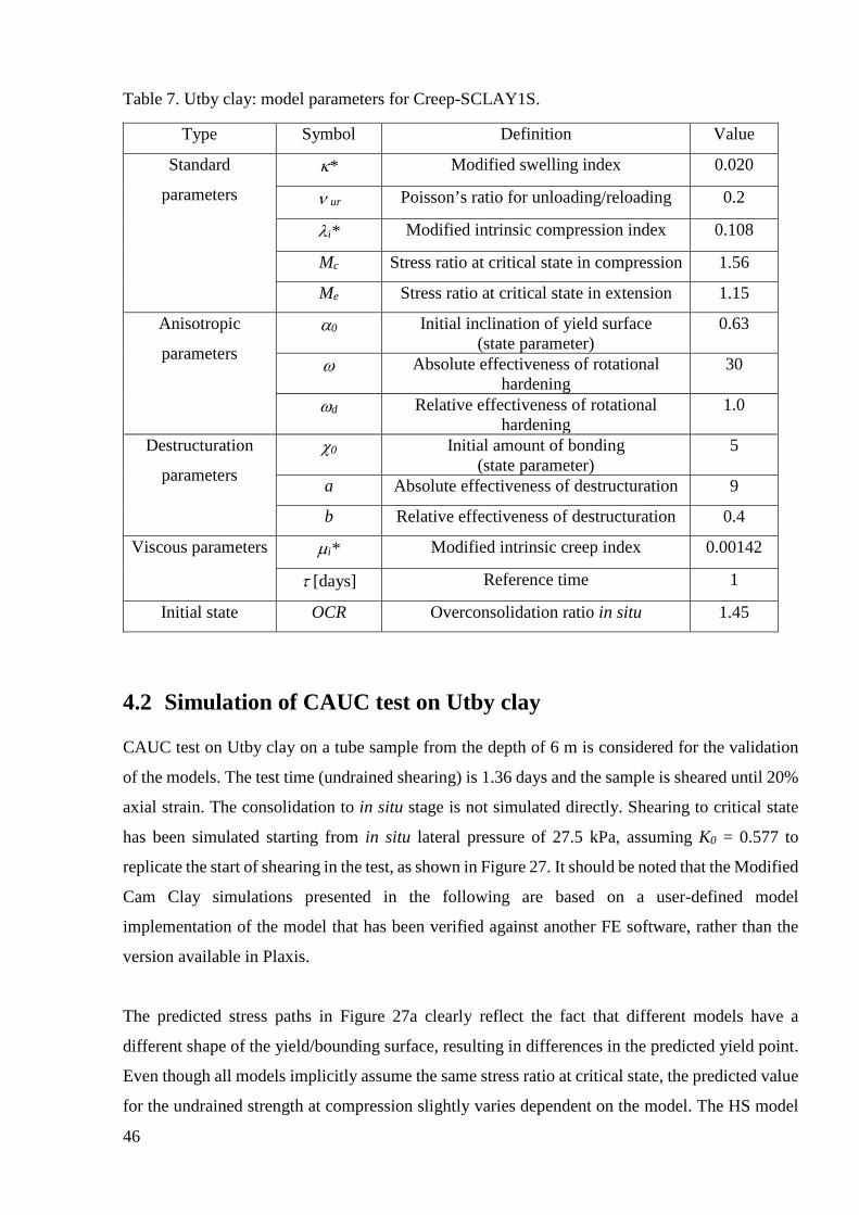
46
Table 7. Utby clay: model parameters for Creep-SCLAY1S.
Type Symbol Definition Value
Standard
parameters κ* Modified swelling index 0.020
ν ur Poisson’s ratio for unloading/reloading 0.2
λi* Modified intrinsic compression index 0.108
Mc Stress ratio at critical state in compression 1.56
Me Stress ratio at critical state in extension 1.15
Anisotropic
parameters α0 Initial inclination of yield surface
(state parameter) 0.63
ω Absolute effectiveness of rotational hardening
30
ωd Relative effectiveness of rotational hardening
1.0
Destructuration
parameters χ0 Initial amount of bonding
(state parameter) 5
a Absolute effectiveness of destructuration 9
b Relative effectiveness of destructuration 0.4
Viscous parameters µi* Modified intrinsic creep index 0.00142
τ [days] Reference time 1
Initial state OCR Overconsolidation ratio in situ 1.45
4.2 Simulation of CAUC test on Utby clay
CAUC test on Utby clay on a tube sample from the depth of 6 m is considered for the validation
of the models. The test time (undrained shearing) is 1.36 days and the sample is sheared until 20%
axial strain. The consolidation to in situ stage is not simulated directly. Shearing to critical state
has been simulated starting from in situ lateral pressure of 27.5 kPa, assuming K0 = 0.577 to
replicate the start of shearing in the test, as shown in Figure 27. It should be noted that the Modified
Cam Clay simulations presented in the following are based on a user-defined model
implementation of the model that has been verified against another FE software, rather than the
version available in Plaxis.
The predicted stress paths in Figure 27a clearly reflect the fact that different models have a
different shape of the yield/bounding surface, resulting in differences in the predicted yield point.
Even though all models implicitly assume the same stress ratio at critical state, the predicted value
for the undrained strength at compression slightly varies dependent on the model. The HS model

47
simulation with Set 2, corresponding to the oedometric parameters, totally fails in predicting both
the stiffness and strength in shearing in triaxial compression. Both creep models predict strain
softening: SSC because of the error in its formulation, and Creep-SCLAY1S due to accounting for
bonding and destructuration. For most geotechnical problems, it is important to get the stiffness
and pore pressures correct at the relevant strain range, typically up to 2% strain. Overall, the HS
model with Set 1 gives a slightly stiffer prediction than the other models. The post-peak stress-
strain curve is not so important, given after the peak the actual samples will have shear banding,
and hence the interpretation of stress and strains based on homogenous soil element is no longer
correct. In sensitive clays, the apparent strain softening is partly constitutive (due to gradual
breakage of the apparent bonding), which the Creep-SCLAY1S can account for, and partly due to
mechanisms of failure forming due to shear banding. Important from practical point of view is the
excess pore pressure prediction, the trend of which only the Creep-SCLAY1S model can
reasonably accurately predict.
An undrained simulation with Mohr Coulomb model would predict a deviator stress at failure of
about 53 kPa for triaxial compression (as the stress path would go straight up until the failure line
at Mc= 1.56). Consequently, the peak value for undrained shear strength cu would be in this case
overpredicted by 15%.
4.3 Simulation of CAUE test on Utby clay
The anisotropically consolidated undrained shearing in triaxial extension is performed on a tube
sample of Utby clay from a depth of 7 m. The duration of the undrained shearing is 2.879 days.
The in situ lateral pressure is 30 kPa with assumed K0 = 0.6 and the sample is sheared until an
axial strain of 15%. Unlike in triaxial compression, the predicted stress paths differ significantly,
as shown in Figure 28a. Overall, the isotropic models give a poor prediction of the stress paths.
Unlike in triaxial compression, theoretically different models assume a different stress ratio at
critical state. The Modified Cam Clay model is least conservative, assuming the same ratio at
critical state in compression and extension. The standard models in Plaxis assume that the friction
angle at critical state is the same in compression and extension, and consequently reach critical
state at a lower stress ratio than the Creep-SCLAY1S model.

48
Figure 27. Utby clay. Simulations of CAUC test at 6 m depth compared to lab data.
In terms of stiffness, there are more significant differences in the stiffness predictions than in
triaxial compression, but again the HS model with Set 2 predicts totally unrealistic stiffness
response. In terms of excess pore pressures, only the Creep-SCLAY1S is able predict the
magnitudes consistent with the experimental results. The models available as standard in Plaxis
overpredict the excess pore pressures, in particular the Soft Soil Creep model.

49
Figure 28. Utby clay. Simulations of CAUE test at 7 m depth compared to lab data.
4.4 Simulations of CRS and IL tests on Utby clay
In order to check the validity of the models for one-dimensional loading, a CRS and an IL tests
are simulated with the standard and advanced models. In the CRS test from a depth of 6 m, the
sample is loaded at constant displacement rate of 0.0024 mm/min, corresponding to a constant
shear rate of 0.72%/hour in the normally consolidated region. Defining starting stress level in CRS
simulations is always tricky, as simulations that start with zero stress cause numerical problems
due to zero strength. In this case, in order to avoid too much nonlinearity in the OC region and to
obtain a reasonable fit to the lab data, the simulations are done by assuming an initial isotropic
stress condition of 25 kPa. As shown in Figure 29a, with the selected set of parameters, most of
the models used give a decent prediction for one-dimensional consolidation, except for the HS
model with parameter Set 1 (fitted with triaxial data), which totally underpredicts the axial strains.

50
In contrast the fit with Set 2, based on IL oedometer test data gives a reasonable prediction, albeit
still underpredicting the axial strains at high stress levels compared to the other models and the
experimental data. In contrast, the other standard models in Plaxis overpredict the axial strains at
high stress levels, because the effects of gradual degradation of the apparent bonding is not
accounted for. The best overall prediction is again given by the Creep-SCLAY1S model.
Finally, an incrementally loaded (IL) oedometer IL test on a tube sample from a depth of 7 m is
loaded in steps as shown in Table 8. Again, the simulations are started by assuming an initial
isotropic effective stress condition of 10 kPa to avoid failure at low stress levels in the OC region.
The overall conclusions are the same as for the CRS test predictions. Again, the HS model
prediction with Set 2, fitted on oedometer test results, gives a reasonable forecast, while the Set 1
results in a gross underprediction of the axial strains. The simulations yet again highlight the
problem with the HS model: different sets of model parameter are needed to match the different
types of experimental results for sensitive clays. This of course reduces the confidence on the
usability of the model for simulating geotechnical problems on soft soils. In Section 5, the
implications at boundary value level are discussed via simplified benchmark simulations.
Table 8. Simulation of IL test on Utby clay.
Duration for each step (days)
Load increment
(kPa)
Total stress (kPa)
0.2535 10 10 0.70 10 20 1.00 20 40 1.09 40 80 2.60 40 120 2.82 40 160 4.95 40 200 6.16 80 280 1.06 100 380

51
Figure 29. Utby clay. Simulations of CRS (at 6m depth) and IL test (at 7 m depth) compared to lab data.

52
5 Benchmark simulations
In order to understand how the choice of the soil model affects the simulations of geotechnical
boundary value problems, in the following three simple benchmark cases are considered: an
embankment on soft clay, a cut excavation on soft clay and a simple cantilever retaining wall
constructed on soft clay. Each benchmark simulation considers first a reference case, followed by
sensitivity study that looks at two extremes, a case when behaviour is largely elastic and a case
when the geostructure has high amount of irrecoverable deformations, but is not quite yet
approaching failure. The soft soil has in all cases been modelled using the parameters of Utby clay
at 6-8 m as given in the previous sections, assuming a bulk density ρ of 1.58 t/m3 for the clay, in
situ K0 of 0.6 and OCR of 1.45. All simulations have been made with Plaxis assuming small strains.
5.1 Embankment benchmark An embankment on Utby clay has been modelled as shown in Figure 30. It is assumed that there
is a 1m thick desiccated crust, underlain by a 39 m deep layer of Utby clay. The groundwater table
is assumed to be at the ground surface. For the sake of simplicity, both the embankment and the
dry crust have been modelled with a linear elastic model, assuming E' = 25000 kPa, ν ' = 0.3 with
a unit weight γ of 20 kN/m3 for the embankment, and E' = 3000 kPa, ν ' = 0.3 and a unit weight
γ of 18 kN/m3 for the dry crust, assuming a K0 = 0.7 for the dry crust. The hydraulic conductivity
of the dry crust is assumed as kx=ky= 8e-4 m/day.
Figure 30. Benchmark embankment.
40 m
80 m
Lateral displacement
Settlement profile Dry crust layer (1m)
Soft soil layer
G.W.L.1 m2 m3 m
Excess PorePressure at 3m below GL
Settlement
1:3
x
y

53
Given the analyses relate to Serviceability Limit State, focusing on deformations, the symmetry of
the problem can be exploited, assuming plane strain conditions. For ultimate limit state, this would
not normally be suitable. The width of the embankment is assumed to be 18 m at the bottom of the
embankment, with side slopes of 1:3. Three different embankment heights are simulated, using a
2m height embankment as a reference case. The lateral boundary is extended to 80m from the
embankment centreline, to prevent any boundary effects. The problem is modelled using 1730
element with 3597 nodes, using 6-noded triangular elements. 6-noded element, rather than 15-
noded element have been selected given reduced integration helps to ensure the computational
stability of coupled consolidation analyses. Due to symmetry, the horizontal displacements are
fixed in the horizontal boundaries and both vertical and horizontal displacement have been fixed
in the bottom. The initial stresses are first created using the K0 procedure, and after that the
embankment is constructed in 50 days. Then, the model is allowed to consolidate, with phases
added for the sake of post-processing after 1 year, 3 years, 5 years and 100 years. Firstly, the
results for 2m height embankment are shown, using all the models, followed by a sensitivity
analyses with different models.
5.1.1 Embankment benchmark with 2 m high embankment The predicted settlement under the centreline (see Figure 30 for the exact location) are plotted in
Figure 31 for 2000 days. The negative sign indicates downwards movement. Given the values for
model parameters have been systematically determined, most models give rather similar
predictions. The idealisation of the soft soil layer with a single set of parameters, and the
assumption of small strains, results in unrealistic settlement magnitudes, but nevertheless enables
to compare different model predictions. As the compressibility was defined based on 1 day IL
tests, in general the two rate-dependent (creep) models give rather similar predictions to the rate-
independent models. At this stage, the consolidation is more pronounced than creep. The
exceptions for good predictions are, yet again, the Hardening Soil model predictions. The HS
model simulation with parameter Set 1, derived based on drained triaxial test results significantly
underestimate the vertical settlements compared to the other models. In contrast, the HS model
prediction with Set 2, fitted for oedometric conditions, are over-predicting the settlement compared
to the other models. This is most likely due to the activation of the deviatoric part of the model,
which for this case with too low value for refE50 results in over-prediction of the settlements. The
results also demonstrate that the embankment on soft soil in this case not a purely one-dimensional
problem, given the same set of parameters (Set 2) resulted in slight underprediction in the element
level (1D) predictions of IL and CRS tests (see Figure 29) compared to the other models.

54
Figure 31. Settlements under the centreline for a 2 m high embankment on Utby clay.
The corresponding long-term predictions up to 100 years have been presented in Figure 32,
together with the excess pore pressures predicted under the centreline of the embankment at a
depth of 3 m. The excess pore pressures are shown as negative values following the sign
convention in the finite elements. In terms of the excess pore pressures, all models excepting HS
model with Set 1 predict that the pore pressures will after an initial reduction due to consolidation
increase for a while, before they start decreasing. This is a consequence of so-called Mandel-Cryer
effect associated with a coupled consolidation formulation. The Creep-SCLAY1S model predicts
2-3 kPa higher excess pore pressures than the other models, which is reflected in the predicted
horizontal movements. Soft Soil and Soft Soil Creep model predictions are almost identical when
the intrinsic value of the modified creep index has been used as input. Normally, however, people
tend to opt for µ* values that correspond to the effective stress level in the problem, and
consequently significantly overpredict the creep strains with the Soft Soil Creep model.
In terms of lateral displacements, the predictions by the models under the toe of the embankment
(see Figure 30 for the exact location) have been presented in Figure 33, corresponding to the end
of construction, 1 year, 3 years and 5 years, respectively. After 5 years, there was no more notable
increase in the lateral displacements. At the end of construction all models, excepting the HS
model, predict rather similar magnitudes for lateral displacements. Hardening Soil model with Set
1 parameter significantly under-predicts, and in contrast with Set 2 significantly over-predicts the
lateral movements compared to the other models. Given the soft soil layer has been assumed to be

55
homogeneous, the maximum value of horizontal movements is predicted to occur at the same
depth with all models. As consolidation (and creep if included in the model) progress, some
differences in the model predictions gradually develop. Overall, the predictions by the Soft Soil,
Soft Soil Creep and the Modified Cam Clay model stay rather similar throughout the process,
indicating that when the input values for soil parameters have been consistently input for similar
type of isotropic models, there are no significant differences between the model predictions.
5.1.2 Sensitivity analyses with different embankment heights In all models used, the predictions are sensitive to the assumed value for OCR. To highlight this
effect, the simulations have been repeated considering both a lower (1 m high) and a higher (3 m
high) embankment. For the sake of clarity, only the prediction with Soft Soil model and Creep-
SCLAY1S model are included in the following. The predicted settlement under the centreline of
the embankment are presented in Figure 34. The settlements are seen to be strongly dependent on
the embankment height: they are predicted to almost double when the height is increased from 1
m to 2 m (moving from largely elastic situation to a situation with irrecoverable deformations),
and further increase to 3 m will again result in a further settlement increase. During the first 2000
days, there is no significant difference in the predictions by the two models, however after 10 years
of consolidation, as shown in Figure 35a, the Creep-SCLAY1S is predicting higher settlement than
the Soft Soil model. In terms of excess pore pressures, the simulations with the two models yield
almost identical results (see Figure 35b), suggesting that with 1 m height, the state of the soft soil
under the embankment load is almost purely elastic. Given the creep models do not have a purely
elastic zone, in time the results start to slightly deviate, with the anisotropic creep model predicting
higher pore pressures than the isotropic Soft Soil model.

56
Figure 32. a) Long-term settlements under the centreline for a 2 m high embankment on Utby clay (top) and the predicted excess pore pressures (bottom) at 3 m below the ground level (time in log-scale).

57
Figure 33. Predicted lateral displacement under the toe of the 2 m high embankment on Utby clay: a) after construction; b) after 1 year; c) after 3 years; and d) after 5 years.
With regards of the lateral displacements, as shown in Figure 36, as expected, the magnitude of
evolving later displacements is highly dependent on the magnitude of loading, and the differences
between the rate-dependent anisotropic creep model and Soft Soil model are apparent already just
after the embankment construction (see Figure 36a), and increase as time passes. It is also clear
from Figure 36 that the results are affected by the assumed boundary conditions, full fixity, at the
bottom of the mesh. In general, it would better to also model the stiff layer (granular materials or
bedrock) underneath the clay, and only apply fixities to that one.

58
Figure 34. Predicted settlements under the centreline of the embankment on Utby clay for three different embankment heights.
Figure 35. Predicted a) long-term settlements, and b) excess pore pressures, under the centreline of the embankment on Utby clay for three different embankment heights (time in log-scale).

59
Figure 36. Predicted lateral displacement under the toe of the embankment on Utby clay: a) after construction; b) after 1 year; c) after 3 years; and d) after 5 years.

60
5.2 Cut excavation benchmark The second benchmark example is a cut excavation on Utby clay as shown in Figure 37. It is
assumed that there is a 1m thick desiccated crust, underlain by a 39 m deep layer of Utby clay.
The groundwater table is assumed to be again at the ground surface. For the sake of simplicity, the
dry crust have been modelled with a linear elastic model, assuming E' = 3000 kPa, ν '=0.3 and a
unit weight γ of 18 kN/m3, with K0 = 0.7 for the dry crust. The hydraulic conductivity of the dry
crust is assumed as kx=ky= 8e-4 m/day.
A 10 m wide cut excavation is considered, with slope 1:3, and two excavation depths: 3m deep
excavation and 5 m deep excavation. These are shown in Figure 37, together with the selected
points for post-processing. The latter case, a 5 m deep excavation, is a critical case where the safety
factor is rather close to 1. The excavation is modelled using 3927 6-noded elements with 8058
nodes, utilizing symmetry. The fixities are the same as in previous example. The model is first
initialized using K0 -procedure, and then the excavation is simulated to occur at a rate of 1 m/week,
assuming the excavation as dry, followed by consolidation.
Figure 37. Benchmark cut excavation.
The predicted heave profile at the bottom of the cut excavation at different points of time are shown
in Figure 38, for the 3 m deep excavation on the left and for the 5 m deep excavation on the right.
Because the input values for the parameters controlling the elastic unloading (κ* or refurE ) were
determined to correspond for large unloading-reloading, the predicted heave will be greater than

61
in reality. Ideally, the soil testing would involve unloading reloading cycle that would correspond
to the expected situation, so that the unloading-reloading modules is determined not only at a
correct stress level but also at a correct amount of unloading.
At the end of excavation process, all models predict rather similar heave, except for the HS model
that predicts heave at totally different magnitudes than the other models, either significantly under-
predicting (with Set 1 parameters) or over-predicting (with Set 2 parameters) compared to the other
models. The Creep-SCLAY1S model is initially predicting marginally more heave that the Soft
Soil, Soft Soil Creep and MCC models, but these catch up in time. After ten years of consolidation,
HS and SS models predict the heave to be the highest at the toe of the excavation, whilst MCC,
Creep-SCLAY1S and Soft Soil Creep models predict the highest values of heave at the centre of
the excavation. When looking at a point underneath the excavation, as shown in Figure 39, the
MCC model and Soft Soil give rather similar predictions, as would be expected given the elastic
laws are almost identical. The same is true for the predicted suction at 8 m below the ground level
plotted in Figure 40.
The predicted lateral displacement profile under the top of the cut slope are plotted in Figure 41,
for the 3 m deep excavation on the left and for 5 m deep excavation on the right. As the movement
is towards the excavation, the values are negative. Again, the predictions by the Hardening Soil
model deviates from the other models, and the Creep-SCLAY1S model predicts somewhat larger
lateral displacements than the Soft Soil, Soft Soil Creep and MCC models. It is also clear from
Figure 41, that the results are affected by the assumed boundary conditions, full fixity, at the
bottom of the mesh, so again it would better to also model the stiff layer (granular materials or
bedrock) underneath the clay and only apply fixities to that one.
The predicted settlement profile at the surface next to the excavation is shown in Figure 42, for the
3 m deep cut excavation on the left and 5 m deep cut excavation on the right respectively. For the
3 m deep (safe) excavation, at the end of the excavation process all models, excepting again the
HS model, predict similar settlements (with negative sign corresponding to downwards
movement). For the 5 m deep excavation, which no longer fulfils the required factors of safety for
stability, the creep models predict larger settlements and the difference is increasing with time,
with the Creep-SCLAY1S predicting the largest settlements after 10 years of consolidation and
creep. In the context of finite elements, failure refers to a case with non-convergence of the
solution.

62
Figure 38. Predicted heave at the bottom of the cut excavation (left) for 3 m deep excavation and (right) for 5 m deep excavation.
Figure 39. Predicted heave as a function of time for a point just below the excavation for a) 3m deep cut excavation and b) 5 m deep cut excavation.

63
Figure 40. Predicted suction as a function of time for a point 8 m below the ground level at the centre of the excavation for a) 3m deep cut excavation and b) 5 m deep cut excavation.
Figure 41. Predicted lateral displacement profile corresponding to the top of the cut excavation (left) for 3 m deep excavation and (right) for 5 m deep excavation.

64
Figure 42. Predicted settlement profile corresponding to the top of the cut excavation (left) for 3 m deep excavation and (right) for 5 m deep excavation.

65
5.3 Cantilever retaining wall benchmark The final benchmark problem to be considered is a simple excavation supported by a sheet pile
wall. The soil stratigraphy and ground water conditions are assumed to be the same as for the
previous benchmark examples. A 15 m long sheet pile, modelled as isotropic elastic material is
considered, assuming sheet pile properties of EA= 7e6 kN/m and EI=1e6 kNm/m is supporting a
20 m wide excavation. In all cases, the interface behaviour is modelled with Mohr Coulomb model,
assuming interface properties of E' =500 kPa, ν ' = 0.2 and a friction angle ϕ' of 38.3°, with an
interface strength reduction of Rinter = 0.6 for all soil models. The default value of 0.1 is taken as
the virtual thickness factor for the interface.
The problem is modelled using 9286 6-noded quadrilateral elements with 18984 nodes, assuming
now symmetrical boundary on the right side. After creation of the in situ stresses via K0 procedure,
the wall is installed by wishing it in place, ignoring any installation effects, followed by excavation
at a rate of 1 m/week. In Sweden, excavations are typically considered as undrained problems, but
given large excavations are often open for a long period, the undrained excavation has been
followed by a consolidation analyses. Two cases are considered, a 2 m deep excavation that is
“safe”, and a 3 m excavation that dependent on the model chosen represents a factor of safety
between 1.0 and 1.5. All models have a FOS>1 for the undrained excavation, but some of the
models predict failure of the excavation during the consolidation process. Again, failure here refers
to non-convergence of the solution. The points of interest have been identified in Figure 43.
Figure 43. Benchmark of cantilever retaining wall on Utby clay.

66
The predicted lateral movements of the sheet pile wall are presented in Figure 44 for the two depths
of excavation: 2 m at the left and 3 m at the right, corresponding to the undrained excavation and
the situation after 1 year of consolidation. As the wall is a cantilever, and the wall itself has a high
stiffness compared to the soft soil, a rotation of the wall around a point close to the bottom of the
wall is predicted. Most of the soil models used predict rather similar lateral movements initially
after the excavation, with HS model predicting again the extremes, dependent on how the
parameters have been determined (Set 1 or Set 2). Smaller lateral movement are predicted with the
HS model when the parameters have been determined based on the triaxial test results, than on the
oedometer tests results. The MCC, Soft Soil and Soft Soil Creep models predict almost identical
lateral movements after the excavation and one year of consolidation. Creep-SCLAY1S model
predicts systematically larger lateral movements than the simple models, and during consolidation
in the case of 3 m deep excavation it even catches up with the Set 2 simulation of the HS model
just by coincidence.
The predicted heave at the bottom of the excavation has been plotted in Figure 45 for the 2 m deep
excavation (on the left) and the 3 m deep excavation (on the right), again after undrained
excavation and after one year of consolidation. Just like in the case of the cut excavation, it is
expected that the heave will be over-predicted with all models, given the parameters controlling
the unloading-reloading response are based on large stress reversals.
The MCC, Soft Soil and Soft Soil Creep models predict almost identical heave after the excavation
(see Figure 45), as expected given the elastic unloading is modelled in a rather similar manner.
Again, the HS model is predicting the two extremes. After one year of consolidation, the Soft Soil
and Soft Soil Creep models predict larger heave than the isotropic MCC model. Creep-SCLAY1S
model is predicting more heave that the isotropic models, but not as much as predicted with HS
model using Set 2 parameters. Whilst most models predict largest heave close to the symmetry
axes, the HS model with Set 2 is predicting the largest values close to the wall, indicating some
numerical instability.
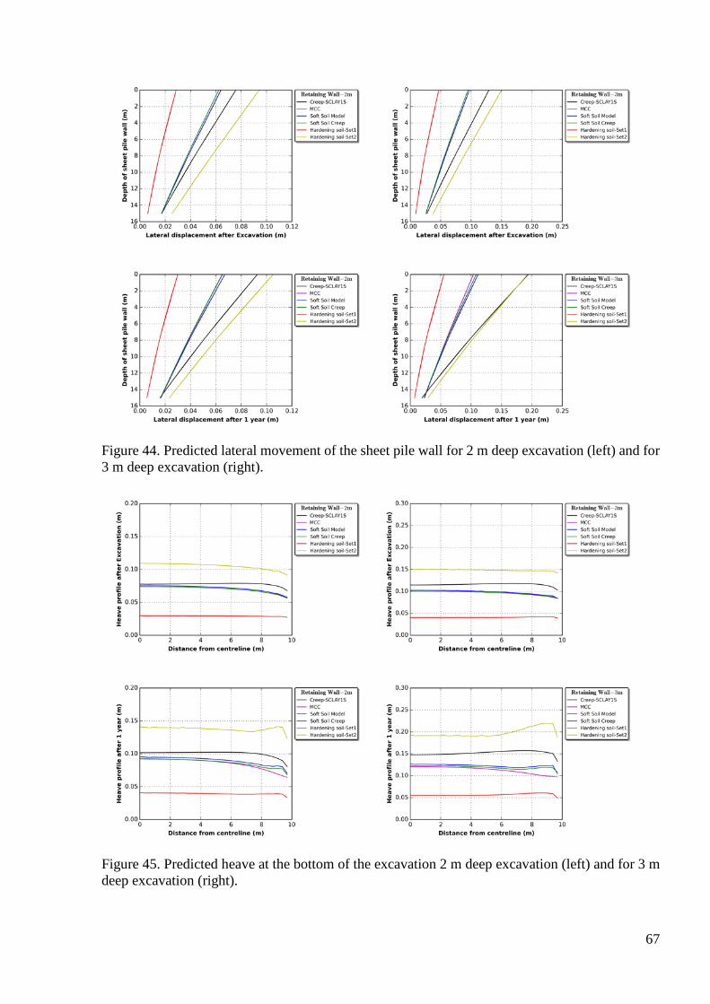
67
Figure 44. Predicted lateral movement of the sheet pile wall for 2 m deep excavation (left) and for 3 m deep excavation (right).
Figure 45. Predicted heave at the bottom of the excavation 2 m deep excavation (left) and for 3 m deep excavation (right).

68
Figure 46. Predicted displacements on ground surface behind the retaining structure for 2 m deep excavation (left) and for 3 m deep excavation (right).
The predicted settlements behind the wall at the ground surface have been presented in Figure 46,
for the 2 m deep excavation (on the left) and the 3m deep excavation (on the right), respectively,
considering the situation immediately after excavation (top) and after 1 year of consolidation
(bottom). Even though rather difficult to see due to the scale, the HS model with Set 2 predicts the
wall to go up immediately after the excavation (as would also be done with the Mohr Coulomb
model), which is unrealistic, whilst the other models predict downwards movement. The largest
settlements are predicted by the Creep-SCLAY1S model after 1 year of consolidation, with the
maximum value just next to the wall. In contrast, the other models predict the maximum value
around 5-10 m from the wall for the 2m deep excavation, and the same is true for the MCC model
for the 3 m excavation.
As seen in Figure 47, the predicted total horizontal stresses (earth pressures) are virtually
independent of the model used, both for the 2m excavation (on the left) and the 3 m excavation
(on the right). The predicted bending moments for both excavation depths have been presented in
Figure 48 for the situation immediately after the undrained excavation (on the left) and after 1 year
of consolidation (on the right). For the sake of clarity, only selected models have been included.
The results for the 2 m deep excavation have been presented with dashed lines and 3 m deep
excavation with solid lines. The largest bending moments in the undrained situation are predicted

69
by the HS model with Set 1 parameters, and overall the variation between the model predictions
is significant. Most notable, however, is how much the bending moments are predicted to increase
during consolidation up to one year for the 3 m deep excavation (see Figure 48, on the right). Now
the HS model with Set 2 gives the largest bending moment predictions together with Creep-
SCLAY1S.
Figure 47. Predicted total stresses for 2 m deep excavation (left) and for 3 m deep excavation (right).
Figure 48. Predicted bending moments immediately after the excavation (left) and after 1 year of consolidation (right).
70
6 Conclusions and recommendations
One of the key steps in geotechnical finite element analyses is the choice of a suitable constitutive
model, and the appropriate selection of the values for model parameters, as the results of the
predictions are highly dependent on these. Different geotechnical problems result in considerably
different effective stress paths, and hence may require different model features to arrive at realistic
results. A major problem is that none of the commercially available soil models implemented in
Finite Element codes have been properly validated for the Scandinavian soft soil conditions.
Furthermore, in the selection of the model, the users too often rely on the recommendations in the
software manuals, which sometimes are totally erroneous for conditions found in Scandinavia. In
contrast, there are recently proposed advanced soil models that have been developed to represent
the response of sensitive soft soils, typically encountered in Scandinavia and North America. These
models, however, require more model parameters than the commercially available standard soil
models. The question is if the extra effort in testing and parameter determination is worth it.
Experimental results on STII samples on Utby clay have been used to systematically derive a
representative set of model parameters for Utby clay, considering the following constitutive
models for the soil: Soft Soil model, Soft Soil Creep model and the Hardening Soil model available
in Plaxis as standard models. In addition, an advanced anisotropic creep model for structured clays
called the Creep-SCLAY1S model has been used for comparison, together with a user-defined
implementation of the isotropic Modified Cam Clay model.
Different soil models have different requirements in terms of the laboratory test results needed for
parameter calibration, as summarised in Table 2. For loading problems, most model parameters
can be derived based on standard test series consisting of oedometer tests (CRS or IL) and
anisotropically consolidated undrained triaxial tests in compression (CAUC). The Hardening Soil
model, ideally, requires consolidated drained triaxial test results, as the elasto-plastic reference
modulus is a drained modulus defined in terms of effective stresses. For soft soils, the consolidated
drained test would ideally be done by starting with anisotropic consolidation to the in situ stress
level before shearing (i.e. CADC test).
For unloading/excavation problems and slope stability problems (if one wants to exploit the
anisotropic strength), additionally, anisotropically consolidated undrained triaxial tests in
extension (CAUE) is needed. For the anisotropic Creep-SCLAY1S model, the CAUE test is also
ideal for calibrating the model parameters related to the evolution of anisotropy. In addition, if
predictions of displacements are deemed important, for unloading problems it is imperative to

71
derive representative model parameters for unloading/reloading. For the latter, a CADC test with
unloading/reloading loop at the appropriate stress level is necessary, regardless of the model used.
The report demonstrates that the determination of parameters for most models is rather straight-
forward. The exceptions are the Hardening Soil model and the Creep-SCLAY1S model. The HS
model requires three reference stiffnesses as input, which means that there are more parameters
than needed for e.g. the Soft Soil model. Furthermore, the parameters derived directly from the
experimental results need to be corrected for the stress-level, hence introducing possibilities for
user errors. Often extensive parameter calibration with simulations are needed. Even then, the
model restrictions disable the input of representative parameter values for Scandinavian clays.
For the Hardening Soil model, two parameter sets were derived: Set 1 based on fit with triaxial
test data and Set 2 based on fit with oedometer test data, as it is not possible to obtain a consistent
parameter set that would represent both. In practice, a “compromise” set is often selected that fails
to represent well any of the stress paths at element level. The Creep-SCLAY1S model, as the most
advanced model, has more parameters than any of the other models used, but many of these are
common parameters, similar to those used in other critical state inspired models (i.e. Soft Soil,
Soft Soil Creep, MCC). There are only three parameters that would require calibration, and recent
research (Gras et al. 2017a) gives guidance on the theoretical ranges of these model parameters.
Based on these powerful tools for automatic parameter optimisation have already been developed
(Gras et al. 2017b).
All soil models considered are sensitive to the value assumed for the apparent preconsolidation
pressure. Given that this parameter is defined in the same way for all models, the same value is
used throughout. It is, however, important to appreciate that in particular for the creep models, the
loading rate (or strain-rate) used in deriving the value is used to fix the input value for the (rate-
dependent) apparent preconsolidation pressure in the time domain by the reference time τ. Hence,
the value for the apparent preconsolidation pressure needs to be derived based on tests where the
loading rate is known, such as the incrementally loaded (IL) oedometer tests. If CRS test results
are used, they need to be appropriately corrected for strain-rates, and even though the Sällfors
(1975) correction is often applied in Sweden, it is not universal. For the creep models, in the
absence of IL tests, CRS tests with different strain rates need to be conducted and compared with
model simulations, before it is possible to do any reliable forward predictions. Therefore, for any
modelling of long-term creep deformations, IL tests are highly recommended.

72
The validation of the selected model parameters is done by simulating at single element level the
various test paths available. Given the model parameters have been systematically derived, most
models are able to reproduce the soil response at the relevant strain level in undrained triaxial
compression, excepting the Set 2 of the HS model (based on oedometer test results), which is
totally off (see Figure 27). There is significantly more deviation when considering undrained
triaxial extension loading paths (see Figure 28). Finally, when incrementally loaded (IL) and
constant rate of displacement (so-called CRS) tests are simulated, this time the HS model with Set
1 parameters (based on triaxial compression) are totally off in terms of predictions (see Figure 29).
The element level simulations clearly demonstrate that the use of the Hardening Soil model is
inappropriate for soft clays, such as Utby clay, as different sets of parameters would be needed for
different standard laboratory stress paths. Furthermore, user errors in stress-scaling the parameters
are common.
In the next stage, the parameters derived and validated for the different soil models are applied in
simple benchmark boundary value problems, considering embankments on soft clay, a cut
excavation in a soft clay and a simple cantilever retaining wall constructed in soft clay. For the
embankment problem on soft clay, when the parameters have been systematically determined,
most models, except for the HS model give rather similar predictions for vertical deformations in
the first 10 years, but in the horizontal displacements the anisotropic creep model gives higher
predictions than the other models. Simulations that compare different embankment heights also
demonstrate that for long term predictions creep is increasingly important with increasing
embankment height.
For the unloading problems, the cut excavation and the cantilever wall, again the HS model gives
predictions that significantly differ from those of the other models, with the two sets representing
the extremes in the undrained situation. For the cut excavation and the simple cantilever wall, the
predicted lateral displacements appear to be mainly dependent on the anisotropy, with significantly
larger displacements predicted by the anisotropic model than the other models. Ignoring anisotropy
is hence not always conservative. The differences increase with the depth of the excavation, and
the differences increase somewhat in time because of creep (see Figure 41 & Figure 44). The
predicted settlements next to the excavation or behind the wall, induced by the lateral movements,
are also affected by the selected model.
Even though the predicted earth pressures behind the cantilever wall are very similar in all cases,
the predicted bending moments are again severely model dependent (see Figure 48). This is due
to the soil-structure interaction, in which the relative stiffness of the soil behind the wall, as

73
compared to the wall stiffness, influences the bending moments in the wall. As a result, with all
models the predicted bending moments are model-dependent and furthermore, the bending
moments increase significantly with time. Therefore, if an excavation is open for any significant
time (a few months upwards), it is necessary to perform consolidation analyses and to be aware
that the predictions are sensitive to the model selected.
It should be noted that the excavation problems above were simulated by all models using model
parameters for unloading/reloading stiffness that relate to rather large unloading/reloading loops.
Therefore, it is expected that the predictions for heave are over-estimated. The predictions could
be improved by using increased (elastic) moduli in areas where small deformations are expected,
see e.g. Figure 14 for example. For any complex geotechnical structure, these areas can be
identified by an iterative process, where after a preliminary simulation, the unloading/reloading
stiffness is increased in areas with small deformations, identified based on e.g. mobilised shear
strains. Even better would be to develop soil models that automatically account for degradation of
small strain stiffness. Unfortunately, the only model available for general use in the commercial
version of the Plaxis is the Hardening Soil model with small strain stiffness (HSsmall), which
suffers from its inability to represent the “large” strain response compared to the other models, as
demonstrated in this report. Developing a model that represents unloading/reloading problems in
soft soils would also need further development in experimental testing. As shown by Wood &
Dijkstra (2015) and Wood (2016), the initial value of small strain stiffness is both stress path
dependent and stress level dependent. Furthermore, it is sensitive to sample disturbance, and very
fresh samples are needed. For modelling, the initial value of small strain stiffness is not enough,
as we need to account for the degradation of the stiffness. Determination of the degradation at a
small stress levels associated with construction on soft soils is error-prone (see the large error bars
in the results of Wood 2016), and further developments on the experimental side are hence
required.
Finally, even though an advanced model, such as the Creep-SCLAY1S, gives a rather good
representation of the soft soil response for standard stress paths, it is not a guarantee that the model
will predict all the complex stress paths associated with complex problems, such as a multi-
propped excavation in an urban area. A challenge in geotechnics is that the (effective) stress paths
cannot be controlled in real boundary value problems. Ideally after initial model predictions, stress
paths are plotted for key locations of the problem. They can subsequently be reproduced in
laboratory, to assess how well the model can predict the measured response at element level. This

74
should then be followed by sensitivity analyses with key model parameters, considering not only
the soil properties, but also the way any structural elements are incorporated.

75
7 References
Andréasson, B. (1979). Deformation characteristics of soft, high-plastic clays under dynamic
loading conditions. PhD thesis, Chalmers University of Technology, Gothenburg, Sweden.
Barnes, G. (1995). Soil mechanics: principles and practice. Macmillan Press Ltd.
Benz, T. (2007). Small strain stiffness of soils and its numerical consequences. PhD Thesis,
University of Stuttgart, Germany.
Bjerrum, L. (1973). Problems of Soil Mechanics and construction on soft soils. State of the art
report to Session IV, 8th ICSMFE, Moscow. NGI Publication No. 100.
Dafalias, Y. F. (1986). An anisotropic critical state soil plasticity model. Mechanics Research
Communications, 13(6), 341-347.
Dawd, S., Trygg, R., & Karstunen, M. (2014). FE analyses of horizontal deformations due to
excavation processes in Gothenburg clay. Proc. 8th European Conference on Numerical
Methods in Geotechnical Engineering, NUMGE 2014), Delft, the Netherlands, Vol. 2, pp.
741-746.
Gens, A., and Nova, R. (1993). Conceptual bases for a constitutive model for bonded soils and
weak rocks. In: Geomechanical Engineering of Hard Soils and Soft Rocks. Edited by A.
Anagnostopoulos, F. Schlosser, N. Kaltesiotis, and R. Frank. A.A. Balkema, Rotterdam, Vol.
1, pp. 485–494
Gras, J.-P., Sivasithamparam, N., Karstunen, M. & Dijkstra, J. (2017a). Permissible range of
model parameters for natural fine-grained materials. Acta Geotechnica. DOI
10.1007/s11440-017-0553-1.
Gras, J. P., Sivasithamparam, N., Karstunen, M., & Dijkstra, J. (2017b). Strategy for consistent
model parameter calibration for soft soils using multi-objective optimisation. Computers and
Geotechnics 90: 164-175.
Grimstad, G., Degado, S. A., Nordal, S., & Karstunen, M. (2010). Modeling creep and rate effects
in structured anisotropic soft clays. Acta Geotechnica, 5(1), 69-81.
Janbu, N. (1977). Slopes and excavations in normally and lightly overconsolidated clays. In
Proceedings of the 9th International Conference on Soil Mechanics and Foundation
Engineering, Tokyo, Vol. 2, pp. 549-566).

76
Karlsson, M., Emdal, A., & Dijkstra, J. (2016). Consequences of sample disturbance when
predicting long-term settlements in soft clay. Canadian Geotechnical Journal 53(12), 1965-
1977.
Karstunen, M., Krenn, H., Wheeler, S. J. Koskinen, M. & Zentar, R. (2005). Effect of anisotropy
and destructuration on the behaviour of Murro test embankment. ASCE International
Journal of Geomechanics 5 (2): 87-97
Karstunen, M., Sivasithamparam, N., Brinkgreve, R.B.J & Bonnier P. (2013). Modelling rate-
dependent behaviour of structured natural clays. Proc. International Conference on
Installation Effects in Geotechnical Engineering, Rotterdam, NL, 23-27 March 2013.
Korhonen, K.-H., & Lojander, M. 1987. Yielding of Perno clay. In: Proc. 2nd International
Conference on Constitutive Laws for Engineering Materials, Tucson, Ariz. Elsevier, N.Y.
Vol. 2, pp. 1249–1255.
Koskinen, M., Karstunen, M., and Wheeler, S.J. (2002). Modelling destructuration and anisotropy
of a natural soft clay. In: Proc. 5th European Conference on Numerical Methods in
Geotechnical Engineering (NUMGE 2002), Paris, 4–6 September, Edited by P. Mestat.
Presses de l’ENPC, Paris. pp. 11–20.
Kempfert, H. G., & Gebreselassie, B. (2006). Excavations and Foundations in Soft Soils. Berlin:
Springer.
Leoni, M., Karstunen, M., & Vermeer, P. A. (2008). Anisotropic creep model for soft soils.
Géotechnique 58(3), 215-226.
Mansikkamäki, J. (2015). Effective stress finite element stability analyses of an old railway
embankment on soft clay. PhD thesis. Tampere University of Technology.
Muir Wood, D. (1990). Soil behaviour and critical state soil mechanics. Cambridge University
Press.
Muir Wood, D. (2016). Analysis of consolidation with constant rate of displacement. Canadian
Geotechnical Journal 53(5): 740-752.
Obrzud, R. F. (2010). On the use of the Hardening Soil Small Strain model in geotechnical
practice. Numerics in Geotechnics and Structures (Eds. Zimmermann, Truty & Podleś).
Elmepress International.

77
Olsson, M. (2010). Calculating long-term settlement in soft clays – with special focus on the
Gothenburg region. Licentiate Thesis Chalmers University of Technology, Gothenburg,
Sweden
Olsson, M. (2013). On Rate-Dependency of Gothenburg Clay. PhD Thesis Chalmers University
of Technology, Gothenburg, Sweden
Parry, R. H. G & Wroth C.P. (1981). Shear stress-strain properties of soft clay. In: Soft Clay
Engineering (Eds. Brand & Brenner). Elsevier, Amsterdam. pp. 311-364.
Perzyna, P. (1963). The constitutive equations for work-hardening and rate sensitive plastic
materials. Proceedings of the Vibration Problems Warsaw, Vol. 3, pp. 281–290
Perzyna, P. (1966). Fundamental problems in viscoplasticity. Advances in Applied Mechanics 9,
243–377
Roscoe, K.H. & Burland, J.B. (1968). On the generalized stress-strain behaviour of 'wet' clay, in:
J. Heyman and F.A. Leckie, eds., Engineering Plasticity (Cambridge Univ. Press,
Cambridge), 535-609.
Schanz, T. (1998). Zur Modellierung des mechanischen verhaltens von Reibungsmaterialien.
Habilitation, Mitteilung 45, Institut fur Geotechnik, Universitaet Stuttgart (in German).
Schanz, T., & Vermeer, P. A. (1996). Angles of friction and dilatancy of sand. Géotechnique 46(1),
145-152.
Schanz, T., & Vermeer, P. A. (1998). On the stiffness of sands. Géotechnique 48, 383-387.
Schanz, T., Vermeer, P. A., & Bonnier, P. G. (1999). The hardening soil model: formulation and
verification. Proceedings of the International Symposium “Beyond 2000 in Computational
Geotechnics”, pp. 281-296.
Sivasithamparam, N., Karstunen, M., & Bonnier, P. (2015). Modelling creep behaviour of
anisotropic soft soils. Computers and Geotechnics 69, 46-57.
Sivasithamparam, N., Karstunen, M., Brinkgreve, R.B.J & Bonnier P. (2013). Comparison of two
anisotropic rate dependent models at element level. Proc. International Conference on
Installation Effects in Geotechnical Engineering, Rotterdam, NL, 23-27 March 2013.
Sällfors, G. (1975). Preconsolidation pressure of soft, high-plastic clays. PhD Thesis, Chalmers
University of Technology, Gothenburg, Sweden.

78
Vermeer, P. A., & Neher, H. P. (1999). A soft soil model that accounts for creep. In Proceedings
of the International Symposium “Beyond 2000 in Computational Geotechnics”, pp. 249-
261.
Vermeer, P. A., Stolle, D. F. E. & Bonnier, P. G. (1998). From the classical theory of secondary
compression to modern creep analysis. Proc. Computer Methods and Advances in
Geomechanics, Wuhan, China, Vol. 4. Rotterdam: Balkema, 2469–2478.
Wheeler, S. J., Näätänen, A. Karstunen, M. & Lojander, M. (2003). An anisotropic elastoplastic
model for soft clays. Canadian Geotechnical Journal 40, 403-418
Wood, T. & Dijkstra J. (2015). On the small strain stiffness of some Swedish clays & its impact on
deep excavations. Research Report. Chalmers University of Technology.
Wood, T. (2016). On the small strain stiffness of some Scandinavian clays and impact on deep
excavations. PhD thesis. Chalmers University of Technology, Gothenburg, Sweden.