1  

Beyond Black-Scholes: The Stochastic Volatility Option Pricing Model and Empirical Evidence from Thailand

Woraphon Wattanatorn1

Abstract

This study compares the performance of two option pricing models, namely

Heston stochastic volatility and Black-Scholes (BS) models(Black & Scholes, 1973). Using SET50-Index option prices, both Heston and Black-Scholes models give pricing errors which are quite large for deep-in-the money options. But the errors of Heston model are smaller for both puts and calls, and for all their moneyness. Based on these findings, this study concludes that the Heston model performs better than the BS model in pricing options in Thailand’s option markets.

Keywords : Stochastic Volatility, Option Pricing Models, Performance Comparison, Thailand’s Option Market

                                                            1 Woraphon Wattanatorn, Ph.D. Student, Faculty of Commerce and Accountancy, Thammasat

University, Bangkok 10200, THAILAND.  

2  

1. Introduction The option pricing model by Black and Scholes (1973) is popular among

academicians and practitioners because it gives closed form formulas for option prices and the sensitivities of their determinants. Hence the Black-Scholes model is very convenient and useful for option pricing and risk management. However, the accuracy of BS model is questionable because it relies on strict assumptions. The BS model assumes that underlying asset prices follow a geometric Brownian motion (GBM) process with known, constant mean and variance. Moreover, it assumes a constant risk-free rate, no transaction costs and continuous trading.

Previous studies reported that the BS model cannot price options accurately. One

of the principal reasons is because its constant volatility assumption is incorrect. The volatility is not constant but moves stochastically over time.(Geske, 1979; Johnson & Shanno, 1987; Rubinstein, 1985; Scott, 1987; Wiggins, 1987)

The purpose of introducing option on SET50 index is to allow investors to hedge

their investment risk, which requires the theoretical pricing model that reflects the actual market prices. Moreover, this pricing model should forecast the future movement of the variables accurately (Khanthavit, 2007). If volatility moves stochastically which violates the constant volatility of BS assumption, BS will misprice. Therefore, the use of hedging parameters obtained by BS model can lead to low hedging efficiency. To capture the changing of volatility, the alternative stochastic volatility option pricing model is more appropriate (Ball & Roma, 1994).

Heston (1993) modifies the BS assumption to accommodate the stochastic

volatility nature of asset returns and derives a model with a closed-form pricing formula(Heston, 1993). It gains popularity over time and the evidence to support its superior performance over the BS model is growing. However, most researches concentrate on developed markets, for example, Bakshi et al (1997) , and Fiorentini et al (2002). The evidence from emerging markets is limited. As emerging markets are characterized by high volatility, high return, less information efficiency, and less transparency(Kearney, 2012), the difference in these characteristics raise an important question as to whether the performance of Heston model holds in emerging markets as in developed markets (Huij & Post, 2011).

This study contributes to the literature in at least four folds. Firstly, it examines

and finds that asset volatility moves stochastically in Thai market so that a model with a stochastic volatility assumption such as Heston’s is more consistent with the data. Secondly, it tests and finds that stochastic volatility significantly affects the performance of option pricing formulas. Thirdly, based on the model comparison using SET 50 index option prices, the study finds the Heston model gives smaller pricing errors and less biased theoretical prices for both put and call options. Fourthly, volatility smiles exist with the Heston model, although less severe than with the BS model.

2. Literature Review 2.1 Stochastic Volatility

In early studies, many researchers documented stochastic volatility for asset prices in developed markets (Geske, 1979; Johnson & Shanno, 1987; Rubinstein, 1985;

3  

Scott, 1987; Wiggins, 1987). Moreover, the stochastic volatility is found to have a mean reversion property (Scott, 1987; Stein & Stein, 1991). More recently researchers uses volatility smile for the BS model from option markets to support stochastic volatility properties of asset prices. For example, Jones (2003) documented an evidence of volatility smile of option on S&P100, which is a high liquidity market, during a sample period of 1986 to 2000 including crisis period(Jones, 2003). Yakoob and Economics (2002) reported volatility smiles in their study of option index on S&P100 and S&P500 using data between 2000 and 2001(Yakoob & Economics, 2002).

Although Heston offered a closed-form pricing formula since 1993, the formula

is difficult to use so that the model is not very popular in the beginning. Until 1997 Bakshi et al. studied the alternative option pricing models, including the Heston model, for S&P500 options using the sample from June 1, 1988 to May 31, 1991. They found volatility smiles for the BS model and concluded the option prices calculated from Heston model were more accurate than those from BS model. Other than US studies, Beber (2001) studied the implied volatility of Italian Stock Market option using MIBO30. It is the most liquid option traded on that market. For the sample between 1995 -1998 the study reported a u-shape relationship between volatility and moneyness for both short and long maturity options. There is an evidence of stochastic volatility in Spain based on the Spanish IBEX-35 (Pena, Rubio, & Serna, 1999). In Japan, the study on Nikkei 225 options after Asian crisis found that the option volatilities exhibited a smile shape (Fukuta & Ma). In the Australia market, Larkin et al. (2012) found a positive relationship between stochastic process and sampling frequency of asset prices. Using ultrahigh frequency data, they documented asymmetric volatility smile on ASX200 -- call options volatility exhibited smile shape only in bear market(Larkin, Brooksby, Lin, & Zurbruegg, 2012).

Fewer studies on stochastic volatility are conducted in emerging markets, but

they conclude the same results. For instance, Singh (2013) studied alternative option pricing models including Heston model in Indian market and found that none can replicate market price. However, Deterministic Volatility Functions (DVF) and Heston models are closer to market prices, compared with other models.

Furthermore, Patakkinang et al. (2012) provides evidence of volatility smile in

Thai market using the SET 50 index option price data from January 2008 to June 2010. The smile serves as evidence supporting the BS model mispricing for Thailand’s options. Hence, the authors warned that BS model should be used carefully, especially for delta and vega analyses.

2.2 Stochastic Volatility Option Pricing Model

The stochastic volatility has a mean reversion pattern, it always reverts to constant long-run mean whenever its current level deviates from the mean value(Hull & White, 1987; Scott, 1987; Stein & Stein, 1991; Wiggins, 1987). Previous empirical studies reported that stochastic volatility option pricing models were more robust, compared with the BS model. Nandi (1998) used high frequency data to study S&P500 index options and found that the stochastic volatility option pricing model offered better pricing performance than BS for out of the money options. Similar evidence was found in European markets(Nandi, 1998). Fiorentini et al. (2002) studied in Spanish market

4  

using daily data that covered pre-crisis period between January 1996 and April 1996 and reported a volatility smile(Fiorentini, Len, & Rubio, 2002). Sigh (2013) documented the volatility smile and pricing bias for the BS model based on NSE index option data in the Indian market(Singh, 2013).

2.3 The Heston Option Pricing Model.

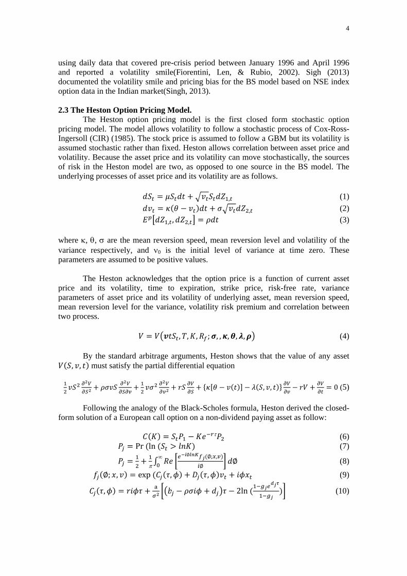
The Heston option pricing model is the first closed form stochastic option pricing model. The model allows volatility to follow a stochastic process of Cox-Ross-Ingersoll (CIR) (1985). The stock price is assumed to follow a GBM but its volatility is assumed stochastic rather than fixed. Heston allows correlation between asset price and volatility. Because the asset price and its volatility can move stochastically, the sources of risk in the Heston model are two, as opposed to one source in the BS model. The underlying processes of asset price and its volatility are as follows.

, (1)

, (2)

, , , (3) where , , are the mean reversion speed, mean reversion level and volatility of the variance respectively, and 0 is the initial level of variance at time zero. These parameters are assumed to be positive values.

The Heston acknowledges that the option price is a function of current asset price and its volatility, time to expiration, strike price, risk-free rate, variance parameters of asset price and its volatility of underlying asset, mean reversion speed, mean reversion level for the variance, volatility risk premium and correlation between two process.

, , , ; , , , , , (4)

By the standard arbitrage arguments, Heston shows that the value of any asset

, , must satisfy the partial differential equation

, , 0 (5)

Following the analogy of the Black-Scholes formula, Heston derived the closed-

form solution of a European call option on a non-dividend paying asset as follow:

(6) Pr ln (7)

; ,∞ (8)

; , exp , , (9)

, 2ln (10)

5  

, (11)

2 (12)

(13)

and 1,2, , , , , and . (14)

3. Research Methodology 3.1 The Data

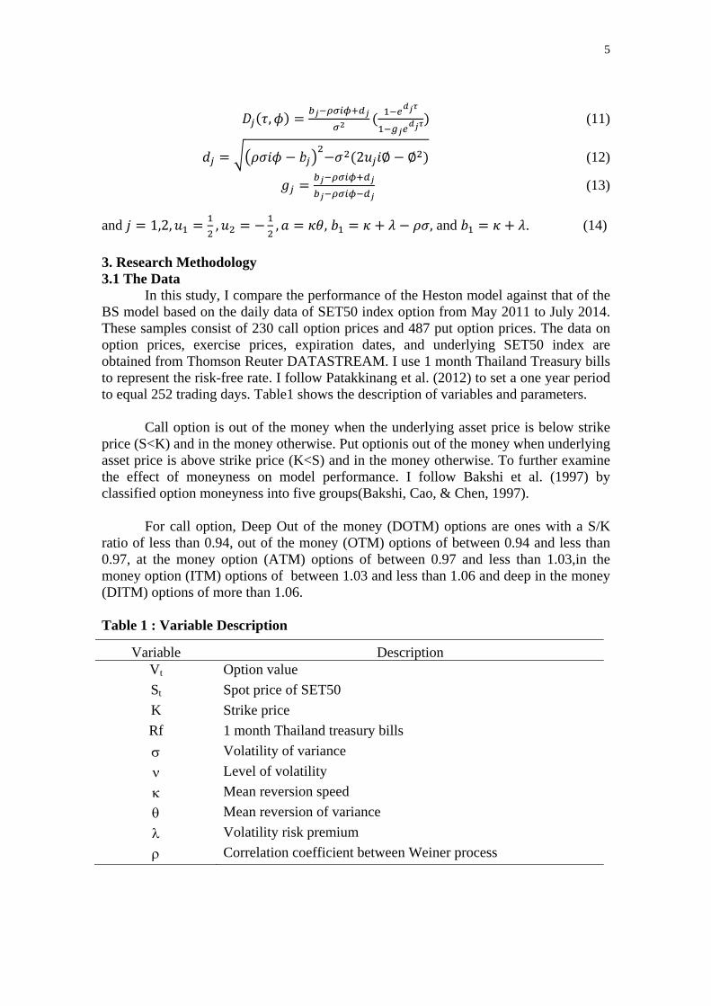
In this study, I compare the performance of the Heston model against that of the BS model based on the daily data of SET50 index option from May 2011 to July 2014. These samples consist of 230 call option prices and 487 put option prices. The data on option prices, exercise prices, expiration dates, and underlying SET50 index are obtained from Thomson Reuter DATASTREAM. I use 1 month Thailand Treasury bills to represent the risk-free rate. I follow Patakkinang et al. (2012) to set a one year period to equal 252 trading days. Table1 shows the description of variables and parameters.

Call option is out of the money when the underlying asset price is below strike price (S<K) and in the money otherwise. Put optionis out of the money when underlying asset price is above strike price (K<S) and in the money otherwise. To further examine the effect of moneyness on model performance. I follow Bakshi et al. (1997) by classified option moneyness into five groups(Bakshi, Cao, & Chen, 1997).

For call option, Deep Out of the money (DOTM) options are ones with a S/K ratio of less than 0.94, out of the money (OTM) options of between 0.94 and less than 0.97, at the money option (ATM) options of between 0.97 and less than 1.03,in the money option (ITM) options of between 1.03 and less than 1.06 and deep in the money (DITM) options of more than 1.06.

Table 1 : Variable Description

Variable Description Vt Option value

St Spot price of SET50

K Strike price

Rf 1 month Thailand treasury bills

Volatility of variance

Level of volatility

Mean reversion speed

Mean reversion of variance

Volatility risk premium

Correlation coefficient between Weiner process

6  

For put option, Deep Out of the money (DOTM) options are ones with a K/S ratio of less than 0.94, out of the money (OTM) options of between 0.94 and less than 0.97, at the money option (ATM) options of between 0.97 and less than 1.03, in the money option (ITM) options of between 1.03 and less than 1.06 and deep in the money (DITM) options of more than 1.06.

Patakkinang et al. studied the sample set including options whose time to

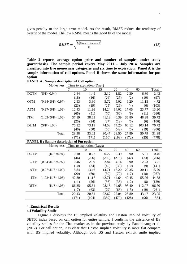
expiration ranged from five days to two months. However, Bakshi et al. (1997) suggested that options of less than six days to expiration may suffer liquidity-related bias. Therefore, in this study the samples will include those options whose time to expiration ranges from seven days to two months. Table2 shows the average option value and number of samples after being filtered the time-to-expiration criterion. Panel A is for call options while Panel B is for put options. There are total of 2,334 option prices, composing of 778 call prices and 1,564 put prices.

Call options are likely to trade at ATM. There are 266 options are traded ATM

in our sample. There are 766 put options in DOTM. This reveals that put options are likely to trade at DOTM. For the same time to maturity, call options are more expensive than put options for DOTM and OTM. For other type of moneyness, put options are more expensive than call options.

3.2 Model Estimation. The Heston model-- , , , ; , , , , , , in equation (4) is the function of underlying asset value, time to expiration, strike price, risk-free rate, and other six model parameters. The six model parameters are estimated using a loss function method suggested by Bakshi et al (1997). The loss function method is numerical estimation that obtains parameter values which minimize the difference between market price and Heston price.

, , , , , , , , ; , , , , , (15) ∑ | , , , , , | (16)

For each day, the objective function in equation (16) will be minimized for the

cross-sectional sum of square error. The numerical method is employed to estimate values of , , , , , .

3.3 Model Performance

I follow previous studies to compare performance by mean percentage pricing error (MPE). The MPE uses actual value rather than absolute values of the forecast errors. Therefore, MPE can provide the direction of biasness in the model(Wilson & Keating, 2001).

∑ (17)

In addition, I use the Root mean square error (RMSE) which is the square root of

the variance of the error that can indicate the absolute fit of the model to actual data. However, the square term of the error gives the high weight to the large error and thus

7  

gives penalty to the large error model. As the result, RMSE reduce the tendency of overfit of the model. The low RMSE means the good fit of the model.

∑

(18)

Table 2 reports average option price and number of samples under study (parenthesis). The sample period covers May 2011 – July 2014. Samples are classified into five moneyness categories and six time to expiration. Panel A is the sample information of call options. Panel B shows the same information for put option. PANEL A : Sample description of Call option

Moneyness Time to expiration (Days) 7 10 15 20 40 60 Total DOTM (S/K<0.94) 2.44 1.49 2.12 1.82 2.30 6.30 2.43 (18) (16) (26) (25) (2) (10) (97)OTM (0.94<S/K<0.97) 2.53 3.30 5.72 5.02 6.20 11.15 4.72 (23) (19) (25) (26) (4) (6) (103)ATM (0.97<S/K<1.03) 12.43 11.96 14.24 14.02 17.05 23.77 13.80 (65) (51) (70) (60) (9) (11) (266)ITM (1.03<S/K<1.06) 37.19 38.63 41.18 40.39 36.80 48.38 39.72 (25) (24) (27) (19) (5) (6) (106)DITM (S/K>1.06) 75.32 73.19 74.53 74.20 66.12 103.14 76.72 (40) (50) (50) (42) (5) (19) (206)

Total 28.38 33.02 30.47 28.50 27.89 50.79 31.38 (171) (171) (160) (198) (172) (25) (778)

PANEL B : Sample description of Put option Moneyness Time to expiration (Days)

7 10 15 20 40 60 Total DOTM (K/S<0.94) 0.10 0.22 0.27 0.39 0.90 5.01 0.46

(46) (206) (230) (219) (42) (23) (766)OTM (0.94<K/S<0.97) 0.46 2.09 2.84 4.14 6.90 12.73 3.71

(10) (34) (45) (33) (10) (9) (141)ATM (0.97<K/S<1.03) 8.84 13.46 14.71 16.20 20.35 30.11 15.79

(20) (60) (80) (72) (17) (18) (267)ITM (1.03<K/S<1.06) 42.80 41.17 42.71 44.64 49.45 55.76 44.38

(11) (26) (36) (36) (12) (8) (129)DITM (K/S>1.06) 86.35 95.61 98.13 94.65 95.40 112.07 96.70

(17) (63) (79) (68) (15) (19) (261)Total 20.43 20.61 22.67 22.04 25.80 43.47 23.05

(171) (104) (389) (470) (428) (96) 1564 4. Empirical Results 4.1Volatility Smile

Figure 1 displays the BS implied volatility and Heston implied volatility of SET50 index based on call option for entire sample. I confirms the existence of BS volatility smiles for the Thai market as in the previous study by Patakkinang et al. (2012). For call option, it is clear that Heston implied volatility is more flat compare with BS implied volatility. Although both BS and Heston exhibit smile implied

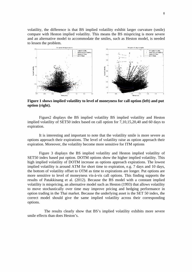
8  

volatility, the difference is that BS implied volatility exhibit larger curvature (smile) compare with Heston implied volatility. This means the BS mispricing is more severe and an alternative model to accommodate the smiles, such as Heston model, is needed to lessen the problem.

Figure 1 shows implied volatility to level of moneyness for call option (left) and put option (right).

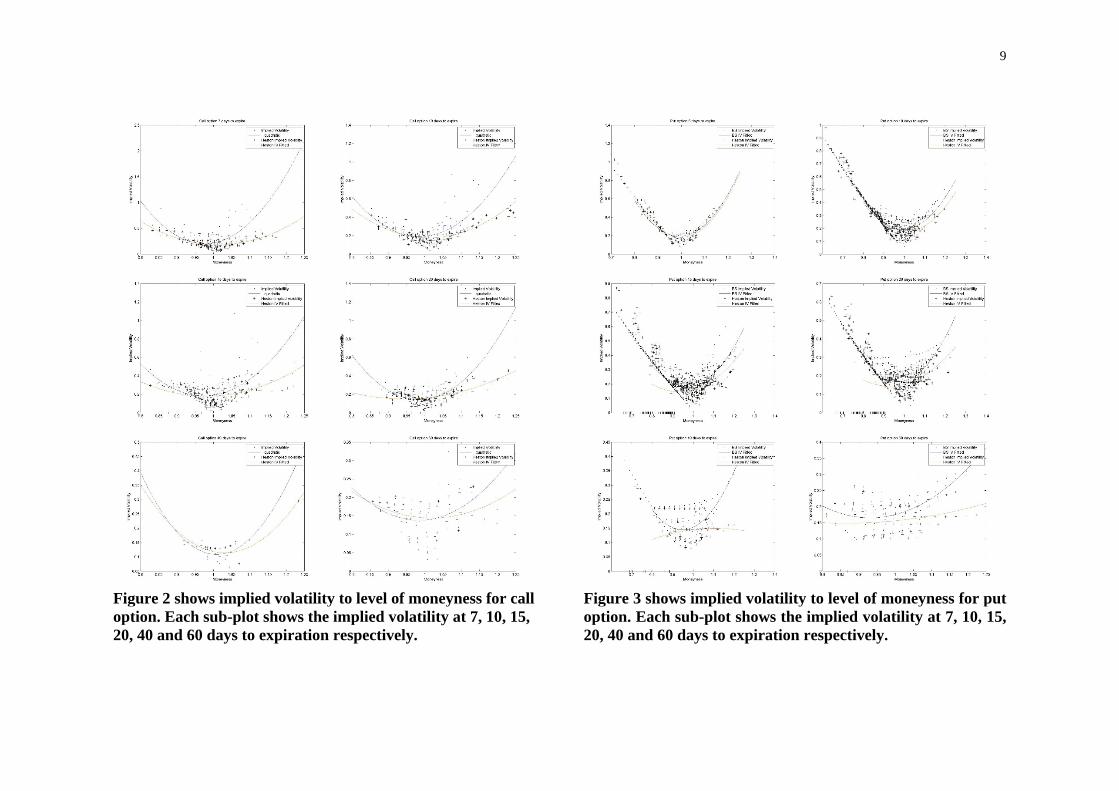
Figure2 displays the BS implied volatility BS implied volatility and Heston

implied volatility of SET50 index based on call option for 7,10,15,20,40 and 60 days to expiration.

It is interesting and important to note that the volatility smile is more severe as

options approach their expirations. The level of volatility raise as option approach their expiration. Moreover, the volatility become more sensitive for ITM options Figure 3 displays the BS implied volatility and Heston implied volatility of SET50 index based put option. DOTM options show the higher implied volatility. This high implied volatility of DOTM increase as options approach expirations. The lowest implied volatility is around ATM for short time to expiration, e.g. 7 days and 10 days, the bottom of volatility offset to OTM as time to expirations are longer. Put options are more sensitive to level of moneyness vis-à-vis call options. This finding supports the results of Patakkinang et al. (2012). Because the BS model with a constant implied volatility is mispricing, an alternative model such as Heston (1993) that allows volatility to move stochastically over time may improve pricing and hedging performance in option trading in the Thai market. Because the underlying asset is the SET 50 index, the correct model should give the same implied volatility across their corresponding options.

The results clearly show that BS’s implied volatility exhibits more severe smile effects than does Heston’s.

9  

Figure 2 shows implied volatility to level of moneyness for call option. Each sub-plot shows the implied volatility at 7, 10, 15, 20, 40 and 60 days to expiration respectively.

Figure 3 shows implied volatility to level of moneyness for put option. Each sub-plot shows the implied volatility at 7, 10, 15, 20, 40 and 60 days to expiration respectively.

10  

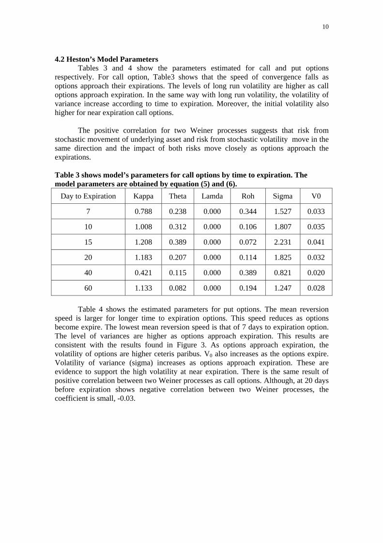
4.2 Heston’s Model Parameters Tables 3 and 4 show the parameters estimated for call and put options

respectively. For call option, Table3 shows that the speed of convergence falls as options approach their expirations. The levels of long run volatility are higher as call options approach expiration. In the same way with long run volatility, the volatility of variance increase according to time to expiration. Moreover, the initial volatility also higher for near expiration call options.

The positive correlation for two Weiner processes suggests that risk from

stochastic movement of underlying asset and risk from stochastic volatility move in the same direction and the impact of both risks move closely as options approach the expirations.

Table 3 shows model’s parameters for call options by time to expiration. The model parameters are obtained by equation (5) and (6).

Day to Expiration Kappa Theta Lamda Roh Sigma V0

7 0.788 0.238 0.000 0.344 1.527 0.033

10 1.008 0.312 0.000 0.106 1.807 0.035

15 1.208 0.389 0.000 0.072 2.231 0.041

20 1.183 0.207 0.000 0.114 1.825 0.032

40 0.421 0.115 0.000 0.389 0.821 0.020

60 1.133 0.082 0.000 0.194 1.247 0.028

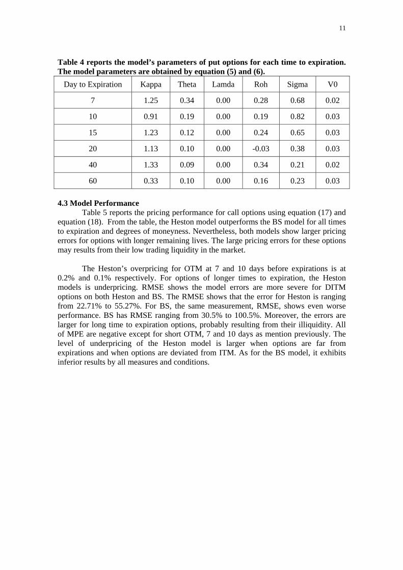
Table 4 shows the estimated parameters for put options. The mean reversion

speed is larger for longer time to expiration options. This speed reduces as options become expire. The lowest mean reversion speed is that of 7 days to expiration option. The level of variances are higher as options approach expiration. This results are consistent with the results found in Figure 3. As options approach expiration, the volatility of options are higher ceteris paribus. V0 also increases as the options expire. Volatility of variance (sigma) increases as options approach expiration. These are evidence to support the high volatility at near expiration. There is the same result of positive correlation between two Weiner processes as call options. Although, at 20 days before expiration shows negative correlation between two Weiner processes, the coefficient is small, -0.03.

11  

Table 4 reports the model’s parameters of put options for each time to expiration. The model parameters are obtained by equation (5) and (6).

Day to Expiration Kappa Theta Lamda Roh Sigma V0

7 1.25 0.34 0.00 0.28 0.68 0.02

10 0.91 0.19 0.00 0.19 0.82 0.03

15 1.23 0.12 0.00 0.24 0.65 0.03

20 1.13 0.10 0.00 -0.03 0.38 0.03

40 1.33 0.09 0.00 0.34 0.21 0.02

60 0.33 0.10 0.00 0.16 0.23 0.03

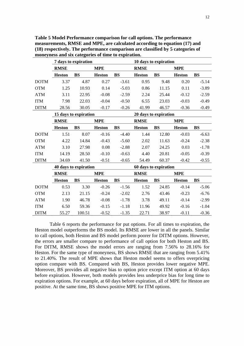
4.3 Model Performance Table 5 reports the pricing performance for call options using equation (17) and equation (18). From the table, the Heston model outperforms the BS model for all times to expiration and degrees of moneyness. Nevertheless, both models show larger pricing errors for options with longer remaining lives. The large pricing errors for these options may results from their low trading liquidity in the market.

The Heston’s overpricing for OTM at 7 and 10 days before expirations is at 0.2% and 0.1% respectively. For options of longer times to expiration, the Heston models is underpricing. RMSE shows the model errors are more severe for DITM options on both Heston and BS. The RMSE shows that the error for Heston is ranging from 22.71% to 55.27%. For BS, the same measurement, RMSE, shows even worse performance. BS has RMSE ranging from 30.5% to 100.5%. Moreover, the errors are larger for long time to expiration options, probably resulting from their illiquidity. All of MPE are negative except for short OTM, 7 and 10 days as mention previously. The level of underpricing of the Heston model is larger when options are far from expirations and when options are deviated from ITM. As for the BS model, it exhibits inferior results by all measures and conditions.

12  

Table 5 Model Performance comparison for call options. The performance measurements, RMSE and MPE, are calculated according to equation (17) and (18) respectively. The performance comparison are classified by 5 categories of moneyness and six categories of time to expiration. 7 days to expiration 10 days to expiration

RMSE MPE RMSE MPE

Heston BS Heston BS Heston BS Heston BS

DOTM 3.37 4.87 0.27 -3.61 0.95 9.48 0.20 -5.14

OTM 1.25 10.93 0.14 -5.03 0.86 11.15 0.11 -3.89

ATM 3.11 22.95 -0.08 -2.59 2.24 25.44 -0.12 -2.59

ITM 7.98 22.03 -0.04 -0.50 6.55 23.03 -0.03 -0.49

DITM 28.56 30.05 -0.17 -0.26 41.99 46.57 -0.36 -0.49

15 days to expiration 20 days to expiration

RMSE MPE RMSE MPE

Heston BS Heston BS Heston BS Heston BS

DOTM 1.51 8.07 -0.16 -4.40 1.44 12.80 -0.03 -6.63

OTM 4.22 14.84 -0.43 -5.60 2.02 11.63 -0.24 -2.38

ATM 3.10 27.98 0.08 -2.88 2.07 24.25 0.03 -1.78

ITM 14.19 28.50 -0.10 -0.63 4.40 20.81 -0.05 -0.39

DITM 34.69 41.50 -0.51 -0.65 54.49 60.37 -0.42 -0.55

40 days to expiration 60 days to expiration

RMSE MPE RMSE MPE

Heston BS Heston BS Heston BS Heston BS

DOTM 0.53 3.30 -0.26 -1.56 1.52 24.85 -0.14 -5.06

OTM 2.13 21.15 -0.24 -2.02 2.76 43.46 -0.23 -6.76

ATM 1.90 46.78 -0.08 -1.78 3.78 49.11 -0.14 -2.99

ITM 6.50 59.36 -0.15 -1.18 11.96 49.92 -0.16 -1.04

DITM 55.27 100.51 -0.52 -1.35 22.71 38.97 -0.11 -0.36 Table 6 reports the performance for put options. For all times to expiration, the

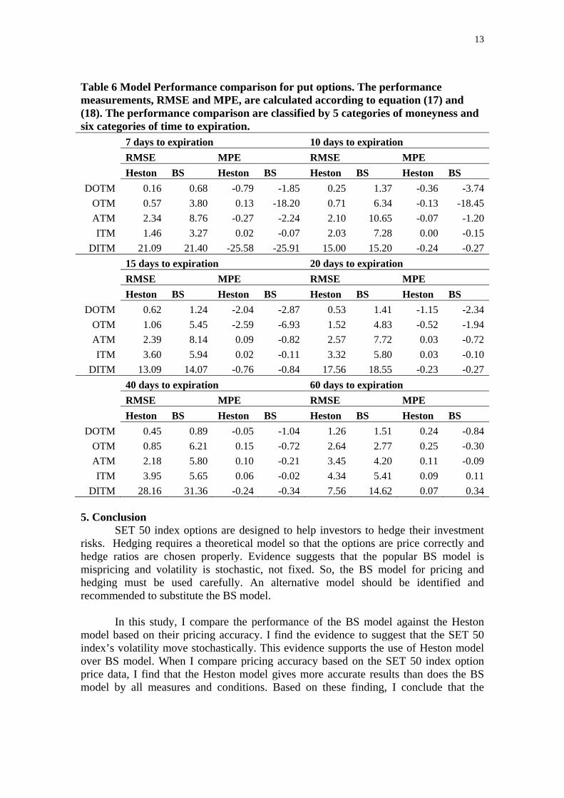
Heston model outperforms the BS model. Its RMSE are lower in all the panels. Similar to call options, both Heston and BS model perform poorer for DITM options. However, the errors are smaller compare to performance of call option for both Heston and BS. For DITM, RMSE shows the model errors are ranging from 7.56% to 28.16% for Heston. For the same type of moneyness, BS shows RMSE that are ranging from 5.41% to 21.40%. The result of MPE shows that Heston model seems to offers overpricing option compare with BS. Compared with BS, Heston provides lower negative MPE. Moreover, BS provides all negative bias to option price except ITM option at 60 days before expiration. However, both models provides less underprice bias for long time to expiration options. For example, at 60 days before expiration, all of MPE for Heston are positive. At the same time, BS shows positive MPE for ITM options.

13  

Table 6 Model Performance comparison for put options. The performance measurements, RMSE and MPE, are calculated according to equation (17) and (18). The performance comparison are classified by 5 categories of moneyness and six categories of time to expiration. 7 days to expiration 10 days to expiration

RMSE MPE RMSE MPE

Heston BS Heston BS Heston BS Heston BS

DOTM 0.16 0.68 -0.79 -1.85 0.25 1.37 -0.36 -3.74

OTM 0.57 3.80 0.13 -18.20 0.71 6.34 -0.13 -18.45

ATM 2.34 8.76 -0.27 -2.24 2.10 10.65 -0.07 -1.20

ITM 1.46 3.27 0.02 -0.07 2.03 7.28 0.00 -0.15

DITM 21.09 21.40 -25.58 -25.91 15.00 15.20 -0.24 -0.27

15 days to expiration 20 days to expiration

RMSE MPE RMSE MPE

Heston BS Heston BS Heston BS Heston BS

DOTM 0.62 1.24 -2.04 -2.87 0.53 1.41 -1.15 -2.34

OTM 1.06 5.45 -2.59 -6.93 1.52 4.83 -0.52 -1.94

ATM 2.39 8.14 0.09 -0.82 2.57 7.72 0.03 -0.72

ITM 3.60 5.94 0.02 -0.11 3.32 5.80 0.03 -0.10

DITM 13.09 14.07 -0.76 -0.84 17.56 18.55 -0.23 -0.27

40 days to expiration 60 days to expiration

RMSE MPE RMSE MPE

Heston BS Heston BS Heston BS Heston BS

DOTM 0.45 0.89 -0.05 -1.04 1.26 1.51 0.24 -0.84

OTM 0.85 6.21 0.15 -0.72 2.64 2.77 0.25 -0.30

ATM 2.18 5.80 0.10 -0.21 3.45 4.20 0.11 -0.09

ITM 3.95 5.65 0.06 -0.02 4.34 5.41 0.09 0.11

DITM 28.16 31.36 -0.24 -0.34 7.56 14.62 0.07 0.34 5. Conclusion

SET 50 index options are designed to help investors to hedge their investment risks. Hedging requires a theoretical model so that the options are price correctly and hedge ratios are chosen properly. Evidence suggests that the popular BS model is mispricing and volatility is stochastic, not fixed. So, the BS model for pricing and hedging must be used carefully. An alternative model should be identified and recommended to substitute the BS model.

In this study, I compare the performance of the BS model against the Heston

model based on their pricing accuracy. I find the evidence to suggest that the SET 50 index’s volatility move stochastically. This evidence supports the use of Heston model over BS model. When I compare pricing accuracy based on the SET 50 index option price data, I find that the Heston model gives more accurate results than does the BS model by all measures and conditions. Based on these finding, I conclude that the

14  

Heston model is superior to the BS model and recommend the Heston model over the BS model for the pricing and hedging the SET 50 index options.

Acknowledgment

The author would like to thank you Professor Anya Khanthavit for ideas and valuable comments. Moreover, I would like to acknowledge his generous support and encouragement.

References Bakshi, G., Cao, C., & Chen, Z. (1997). Empirical Performance of Alternative Option

Pricing Models. The Journal of Finance, 52(5), 2003-2049. doi: 10.1111/j.1540-6261.1997.tb02749.x

Ball, C. A., & Roma, A. (1994). Stochastic volatility option pricing. Journal of Financial and Quantitative Analysis, 29(04), 589-607.

Black, F., & Scholes, M. (1973). The Pricing of Options and Corporate Liabilities. The Journal of Political Economy, 81(3), 637-654. doi: doi: 10.2307/1831029

Fiorentini, G., Len, A., & Rubio, G. (2002). Estimation and empirical performance of Heston's stochastic volatility model: the case of a thinly traded market. Journal of Empirical Finance, 9(2), 225-255. doi: http://dx.doi.org/10.1016/S0927-5398(01)00052-4

Fukuta, Y., & Ma, W. Implied volatility smiles in the Nikkei 225 options. Applied Financial Economics, 23(9), 789-804. doi: 10.1080/09603107.2013.767975

Geske, R. (1979). The valuation of compound options. Journal of Financial Economics, 7(1), 63-81. doi: http://dx.doi.org/10.1016/0304-405X(79)90022-9

Heston, S. (1993). A closed-form solution for options with stochastic volatility with applications to bond and currency options. Review of Financial Studies, 6(2), 327-343. doi: 10.1093/rfs/6.2.327

Huij, J., & Post, T. (2011). On the performance of emerging market equity mutual funds. Emerging Markets Review, 12(3), 238-249. doi: http://dx.doi.org/10.1016/j.ememar.2011.03.001

Hull, J., & White, A. (1987). The pricing of options on assets with stochastic volatilities. The Journal of Finance, 42(2), 281-300.

Johnson, H., & Shanno, D. (1987). Option Pricing when the Variance is Changing. The Journal of Financial and Quantitative Analysis, 22(2), 143-151. doi: 10.2307/2330709

Jones, C. S. (2003). The dynamics of stochastic volatility: evidence from underlying and options markets. Journal of Econometrics, 116(1โ€“2), 181-224. doi:

http://dx.doi.org/10.1016/S0304-4076(03)00107-6 Kearney, C. (2012). Emerging markets research: Trends, issues and future directions.

Emerging Markets Review, 13(2), 159-183. doi: http://dx.doi.org/10.1016/j.ememar.2012.01.003

Khanthavit, A. (2007). An Indirect Approach to Identify the "Correct"Option Pricing Model from Competing Assumptions for Underlying Asset Price, Manuscript, Thammasat University, Bangkok (in Thai).

Larkin, J., Brooksby, A., Lin, C. T., & Zurbruegg, R. (2012). Implied volatility smiles, option mispricing and net buying pressure: evidence around the global financial crisis. Accounting & Finance, 52(1), 47-69. doi: 10.1111/j.1467-629X.2011.00419.x

15  

Nandi, S. (1998). How important is the correlation between returns and volatility in a stochastic volatility model? Empirical evidence from pricing and hedging in the S&P 500 index options market. Journal of Banking & Finance, 22(5), 589-610.

Pena, I., Rubio, G., & Serna, G. (1999). Why do we smile? On the determinants of the implied volatility function. Journal of Banking & Finance, 23(8), 1151-1179. doi: http://dx.doi.org/10.1016/S0378-4266(98)00134-4

Rubinstein, M. (1985). Nonparametric Tests of Alternative Option Pricing Models Using All Reported Trades and Quotes on the 30 Most Active CBOE Option Classes from August 23, 1976 through August 31, 1978. The Journal of Finance, 40(2), 455-480. doi: 10.1111/j.1540-6261.1985.tb04967.x

Scott, L. O. (1987). Option Pricing when the Variance Changes Randomly: Theory, Estimation, and an Application. The Journal of Financial and Quantitative Analysis, 22(4), 419-438. doi: 10.2307/2330793

Singh, V. K. (2013). Empirical Performance of Option Pricing Models: Evidence from India

International Journal of Economics and Finance, 5(2). Stein, E. M., & Stein, J. C. (1991). Stock price distributions with stochastic volatility: an

analytic approach. Review of Financial Studies, 4(4), 727-752. Wiggins, J. B. (1987). Option values under stochastic volatility: Theory and empirical

estimates. Journal of Financial Economics, 19(2), 351-372. doi: http://dx.doi.org/10.1016/0304-405X(87)90009-2

Wilson, J. H., & Keating, B. (2001). Business Forecasting with ForecastX: McGraw-Hill Higher Education.

Yakoob, M. Y., & Economics, D. U. D. o. (2002). An Empirical Analysis of Option Valuation Techniques Using Stock Index Options.