Beyond Competitive Devaluations:

The Monetary Dimensions of Comparative Advantage

Paul R. Bergin Department of Economics, University of California at Davis, and NBER

Giancarlo Corsetti

Cambridge University and CEPR

This draft March 2016

Abstract

Motivated by the long-standing debate on the pros and cons of competitive devaluation, we propose a new perspective on how monetary and exchange rate policies can contribute to a country’s international competitiveness. We refocus the analysis on the implications of monetary stabilization for a country’s comparative advantage. We develop a two-country New-Keynesian model allowing for two tradable sectors in each country: while one sector is perfectly competitive, firms in the other sector produce differentiated goods under monopolistic competition subject to sunk entry costs and nominal rigidities, hence their performance is more sensitive to macroeconomic uncertainty. We show that, by stabilizing markups, monetary policy can foster the competitiveness of these firms, encouraging investment and entry in the differentiated goods sector, and ultimately affecting the composition of domestic output and exports. Keywords: monetary policy, production location externality, firm entry, optimal tariff JEL classification: F41

We thank our discussants Matteo Cacciatore, Fabio Ghironi, Paolo Pesenti, and Hélène Rey, as well as Mary Amiti, Giovanni Maggi, Sam Kortum, Kim Ruhl, and seminar participants at the 2013 NBER Summer Institute, the 2013 International Finance and Macro Finance Workshop at Sciences Po Paris, the 2013 Norges Bank Conference The Role of Monetary Policy Revisited, the 2014 ASSA meetings, the 2014 West Coast Workshop on International Finance and Open Economy Macroeconomics, the CPBS 2014 Pacific Basin Research Conference, the 2014 Banque de France PSE Trade Elasticities Workshop, Bank of England, Bank of Spain, London Business School, New York FED the National University of Singapore, Universidade Nova de Lisboa, and the Universities of Cambridge, Wisconsin, and Yale for comments. We thank Yuan Liu, Riccardo Trezzi and Jasmine Xiao for excellent research assistance. Giancarlo Corsetti acknowledges the generous support of the Keynes Fellowship at Cambridge University, the Cambridge Inet Institute and Centre for Macroeconomics. Paul R. Bergin, Department of Economics, University of California at Davis, One Shields Ave., Davis, CA 95616. Phone: (530) 752-0741. Email: prbergin@ucdavis.edu. Giancarlo Corsetti, Faculty of Economics, Cambridge University Sidgwick Avenue Cambridge CB3 9DD United Kingdom. Phone: +44(0)1223525411. Email: gc422@cam.ac.uk.

1

1. Introduction

This paper offers a new perspective on how monetary and exchange rate policy can

strengthen a country’s international competitiveness. Conventional policy models

emphasize the competitive gains from currency devaluation, which lowers the relative cost

of producing in a country over the time span that domestic wages and prices are sticky in

local currency. In modern monetary theory and central bank practice, however, reliance on

devaluation to boost competitiveness is not viewed as a viable policy recommendation on

two accounts. First, it may be interpreted as a strategic beggar-thy-neighbor measure,

inviting retaliation up to causing currency wars, and second, it is bound to worsen the

short-run trade-offs between inflation and unemployment. Conversely, recent contributions

to the New Open Economy Macro (NOEM) and New-Keynesian (NK) tradition stress that

monetary policymakers can exploit a country’s monopoly on its terms of trade. As this

typically means pursuing a higher international price of home goods, the implied policy

goal appears to be the opposite of improving competitiveness.1 In this paper, we take a

different perspective, and explore the relevance for a country’s comparative advantage of

adopting monetary and exchange rate regimes which may or may not deliver efficient

macroeconomic stabilization.

We motivate our analysis with the observation that monetary policy aimed at

stabilizing marginal costs and demand conditions at an aggregate level (weakening or

strengthening the exchange rate in response to cyclical disturbances) is likely to have

asymmetric effects across sectors. Stabilization policy can be expected to be more

consequential in industries where firms face higher nominal rigidities together with

significant up-front investment to enter the market and price products---features typically

associated with differentiated manufacturing goods. To the extent that monetary policy

ensures domestic macroeconomic stability, it creates favorable conditions for firms’ entry

1 In virtually all contributions to the new-open economy macroeconomics and New-Keynesian literature, the trade-off between output gap and exchange rate stabilization is mainly modeled emphasizing a terms-of-trade externality (see Obstfeld and Rogoff (2000) and Corsetti and Pesenti (2001, 2005), Canzoneri et al. (2005) in the NOEM literature, as well as Benigno and Benigno (2003), and Corsetti et al. (2010) in the New-Keynesian literature, among others). Provided the demand for exports and imports is relatively elastic, an appreciation of the terms of trade of manufacturing allows consumers to substitute manufacturing imports for domestic manufacturing goods, without appreciable effects in the marginal utility of consumption, while reducing the disutility of labor. The opposite is true if the trade elasticity is low.

2

in such industries, with potentially long-lasting effects on their competitiveness, and thus

on the weight of their production in domestic output and exports.

To illustrate our new perspective on the subject, we specify a stochastic general-

equilibrium monetary model of open economies with incomplete specialization across two

tradable sectors. In one sector, conventionally identified with manufacturing, firms produce

an endogenous set of differentiated varieties operating under imperfect competition; in the

other sector, firms produce highly substitutable, non-differentiated goods---for simplicity

we assume perfect competition. The key distinction between these sectors is that

differentiated good producers face a combination of nominal rigidities and sunk entry costs

that make them more sensitive to macroeconomic uncertainty.

The key result from our model is that efficient stabilization regimes affect the

average relative price of a country’s differentiated goods in terms of its nondifferentiated

goods, and, relative to the case of insufficient stabilization, confer comparative advantage

in the sale of differentiated goods both at home and abroad. Underlying this result is a

transmission channel at the core of modern monetary literature: in the presence of nominal

rigidities, uncertainty implies the analog of a risk premium in a firm’s optimal prices,

depending on the covariance of demand and marginal costs (See Obstfeld and Rogoff 2000,

Corsetti and Pesenti 2005 and more recently Fernandez-Villaverde et al. 2011). We show

that, by impinging on this covariance, and thus on the variability of the ex-post markups,

optimal monetary policy contributes to manufacturing firms setting efficiently low,

competitive prices on average, with a positive demand externality affecting the size of the

market. A large market in turn strengthens the incentive for new manufacturing firms to

enter, see e.g., Bergin and Corsetti (2008) and Bilbiie, Ghironi and Melitz (2008). An

implication of the theory that is relevant for policy-related research is that, everything else

equal, countries with a reduced ability to stabilize macro shocks will tend to specialize

away from differentiated manufacturing goods, relative to the countries that use their

independent monetary policy to pursue inflation and output gap stabilization.

We calibrate our model, including TFP shocks based on novel estimates of the TFP

process for differentiated and non-differentiated sectors in the US vis-à-vis an aggregate of

European countries. In the calibrated model we find that the unconditional mean of the

share of a country’s exports in differentiated goods substantially falls if a country replaces

3

optimal monetary rules with a unilateral peg implying insufficient output gap stabilization.

The size of the contraction, between one and two percent in most calibrations, is consistent

with the presumption that monetary policy regimes may be expected to have a moderate

impact on real allocation, but we also show economies in which the contraction is as high

as 9 percent.

Our model is related to closed-economy literature analyzing stabilization in multi-

sector economy (such as Bodenstein, et al., 2008), with a key difference. Via market

dynamics, trade costs create an externality that amplifies the implications of stabilization

policies for firm entry and the sectoral composition of national output. This externality

markedly differentiates the present paper from earlier work of ours, also analyzing the

relevance of monetary policy for market dynamics in a closed economy context. From the

perspective of trade theory, our analysis is related to leading work on tariffs by Ossa (2011),

which nonetheless abstracts from nominal rigidities and other distortions that motivate our

focus on stabilization policy. Ossa’s paper, like ours, models a country’s comparative

advantage drawing on the literature on the ‘home market effect’ after Krugman (1980),

implying production relocation externalities associated with the expansion of

manufacturing.2

The mechanisms by which monetary policy may influence comparative advantage

are of course relevant also for stabilization policies relying on fiscal and financial

instruments. Taxes and subsidies may contribute to demand and markup stabilization,

containing the distortions due to nominal price stickiness and thus, according to our core

argument, misallocation across sectors. While, everything else equal, inefficient monetary

stabilization (e.g., deriving from adopting a fixed exchange) may hamper comparative

advantage in manufacturing, substitution among policy instruments may make up for

2 According to the ‘home market effect,’ the size of the market (i.e. a high demand) is a source of comparative advantage in manufacturing. In this literature, the social benefits from gaining comparative advantage in the manufacturing sector stem from a ‘production relocation externality.’ In the presence of such an externality, acquiring a larger share of the world production of differentiated goods produces welfare gains due to savings on trade costs. Our work is also related to Corsetti et al. (2007), which considers the role of the home market effect in a real trade model, as well as Ghironi and Melitz (2005). We differ in modeling economies with two tradable sectors, as well as considering the implications of price stickiness and monetary policy.

4

constraints on monetary policy. Our analysis shows a specific reason why exploiting a wide

range of stabilization instruments is particularly valuable.

The text is structured as follows. The next section describes the model, and section

3 derives analytical results for a simplified version. Section 4 uses stochastic simulations to

demonstrate a broader set of implications. Section 5 concludes.

2. Model

In what follows, we develop a two-country monetary model, introducing a key

novel element in the way we specify the goods market structure. Namely, each country—

home and foreign--- produces two types of tradable goods. The first type comes in

differentiated varieties produced under monopolistic competition. In this market, firms

face entry costs and nominal rigidities. The second type of good is produced by perfectly

competitive firms, and is modeled according to the standard specification in real business

cycle models. For this good, there is perfect substitutability among producers within a

country (indeed, the good is produced under perfect competition), but imperfect

substitutability across countries, as summarized by an Armington elasticity.

In the text we present the households’ and firms’ problems as well as the monetary

and fiscal policy rules from the vantage point of the home economy, with the understanding

that similar expressions and considerations apply to the foreign economy---foreign

variables are denoted with a “*”. Also, in presenting the model we focus on the case of

balanced trade, which also provides the baseline for our simulation---the bond economy

case is presented in the appendix.

2.1. Goods consumption demand and price indexes

Households consume goods from two sectors. The D sector consists of differentiated

varieties of manufacturing good, which are produced by n and n* monopolistically

competitive firms in the home and foreign country, respectively (from now on, foreign

variables will be denoted with an asterisk). Each variety in the D sector is an imperfect

substitute for any other variety in this sector, either of home or foreign origin, with

elasticity ϕ. The N sector consists of non-differentiated goods, produced by perfectly

5

competitive firms. The home and foreign versions of the N good are imperfect substitutes

for each other, with elasticity η. For convenience, hereafter we may refer to the first sector

as ‘manufacturing.’

The overall consumption index is specified:

CtC

D ,t C

N ,t1

,

where

* 11 1

,

0 0

t tn n

D t t tC c h dh c f df

is the index over the home and foreign varieties of manufacturing good, c(h) and c(f), and

CN ,t

1

CH ,t

1

1 1

CF ,t

1

1

is the index over goods differentiated only by country of origin, with ν accounting for the

weight on domestic goods. The corresponding consumption price index is

1, ,

11

D t N tt

P PP

, (1)

where

1

1 1* 1,D t t t t tP n p h n p f

(2)

is the index over the prices of all varieties of home and foreign manufacturing goods, and

1

1 1 1, , 1 ,N t H t FtP P P (3)

is the index over the prices of home and foreign non-differentiated goods.

These definitions imply relative demand functions for domestic residents:

, ,( ) /t t D t D tc h p h P C

(4)

, ,( ) /t t D t D tc f p f P C

(5)

, ,/D t t t D tC P C P (6)

, ,1 /N t t t N tC PC P (7)

, , , ,/H t H t N t N tC P P C

(8)

6

, , , ,1 /F t F t N t N tC P P C

. (9)

2.2. Home households’ problem

The representative home household derives utility from consumption (C), and from

holding real money balances (M/P); it derives disutility from labor (l). The household

derives income by selling labor at the nominal wage rate (W); it receives real profits t

from home firms as defined below, and interest income (iB) on holding domestically traded

bonds, which are in zero net supply. It pays lump-sum taxes (T).

Household optimization for the home country may be written:

00

max , ,t tt t

t t

ME U C l

P

where utility is defined by

1 11 1ln

1 1t

t t tt

MU C l

P

,

subject to the budget constraint:

1 1 11t t t t t t t t t t tPC M M B i B Wl T .

Above, σ denotes risk aversion and ψ the inverse of the Frisch elasticity. Defining t t tPC ,

optimization implies an intertemporal Euler equation:

1

t

1 it E

t

1

t1

(10)

a labor supply condition:

t t tW l (11)

and a money demand condition:

1 t

t tt

iM

i

. (12)

The problem and first order conditions for the foreign household are analogous.

2.3. Home firm problem and entry condition in the differentiated good sector

In the differentiated goods sector, production is linear in labor:

7

,t D t ty h l h , (13)

where l(h) is the labor employed by firm h, and D is stochastic technology common to all

differentiated goods producers in the country. Exports involve an iceberg trade cost, D , so

that

*1t t D ty h d h d h , (14)

where , ,( ) ( ) ( )t t AC t K td h c h d h d h is total demand for the product in the home country,

for use in consumption, adjustment costs, and entry costs, respectively; *td h is the

corresponding demand for home goods abroad. Firm profits are computed as:

* *,/t t t t t t t t t p th p h d h e p h d h W y h AC h . (15)

To set up a firm, managers incur a one-time sunk cost, , and production starts

with a one-period lag. In each period, all firms operating in the differentiated good sector

face an exogenous probability of exit , so that a fraction of all firms exogenously stop

operating each period. Thus the value function of firms that enter the market in period t

may be represented as the discounted sum of profits of domestic sales and export sales, i,

0

1s t s

t t t ss t

v h E h

,

and, with free entry, new producers will invest until the point that a firm’s value equals the

entry sunk cost. The stock of firms at each point in time is:

. (16)

We include a congestion externality in the entry, represented as an adjustment cost that is a

function of the number of new firms.

1

tt

t

neK K

ne

.

The congestion externality plays a similar role as the adjustment cost for capital standard in

business cycle models, which moderates the response of investment to match dynamics in

data. In a similar vein, we calibrate the adjustment cost to match data on the dynamics of

new firm entry. We generally specify entry costs as consisting of labor units and/or

investment in differentiated goods units. The entry condition may be written

1t K t K Dt tv h W P K , (17)

K

1 1t t tn n ne

8

where K =1 is the case of entry costs in labor units, and K =0 is the case of goods units.

The goods component of the entry cost falls on both domestically produced and imported

goods, in similar proportion as consumption:

, ,( ) / 1K t t D t K t td h p h P ne K

(18)

, ,( ) / 1K t t D t K t td f p f P ne K

. (19)

The home firm h sets a price p(h) in domestic currency units for domestic sales.

Under the assumption of producer currency pricing, this implies a foreign currency price

* 1 /t D t tp h p h e , (20)

where the nominal exchange rate, e, is defined as home currency units per foreign currency

unit. Firms face a nominal cost of adjusting prices

2

1

12

tPt t t

t

p hAC h p h y h

p h

. (21)

For the sake of tractability, we follow Bilbiie et al. (2008) in assuming that new entrants

inherit from the price history of incumbents the same price adjustment cost, and so make

the same price setting decision. The aggregate value of the price adjustment costs is:

t t tAC h n AC h . (22)

To adjust their price, firms use final goods according to:

, , , ,( ) /AC t t M t AC D td h p h P D

(23)

, , , ,( ) /AC t t M t AC D td f p f P D

(24)

, , ,/AC D t t t D tD P AC P (25)

, , ,1 /AC N t t t N tD P AC P (26)

, , , , , ,/AC H t H t N t AC N tD P P D

(27)

, , , , , ,1 /AC F t F t N t AC N tD P P D

. (28)

similar to the composition of equations (4)-(9).

Maximizing firm value subject to the constraints above leads to the price setting

equation:

9

2 2

1 1 1

2

1 11

11 1

1 2 1

11

t t tt Pt t P

t t t t

t ttPt

t t t

p h p h p hWp h p h

p h p h p h

p h p hE

p h p h

(29)

where the optimal pricing is a function of the stochastically discounted demand faced by

producers of domestic differentiated goods,

, , , 1 1,

* * * *, , , 11*

,

1

11 1 .

tt D t AC D t K t t

M t

D tD t AC D t tD K t t

M tt

p hC D ne K

P

p hC D ne K

e P

.

Note that, since households own firms, they receive firm profits but also finance the

creation of new firms. In the household budget, the net income from firms may be written:

t t t t tn h nev h .

2.4. Home firm problem in the undifferentiated good sector

In the second sector firms are assumed to be perfectly competitive in producing a

good differentiated only by country of origin. The production function for the home non-

differentiated good is linear in labor:

, , ,H t H t H ty l , (30)

where ,H t is subject to shocks. It follows that the price of the homogeneous goods in the

home market is equal to marginal costs:

, ,/H t t H tp W . (31)

An iceberg trade cost specific to the non-differentiated sector implies prices of the home

good abroad are

p*H ,t

p*H ,t

1N / e

t. (32)

Analogous conditions apply to the foreign non-differentiated sector.

2.5. Monetary and fiscal policy

10

Monetary authorities are assumed to pursue an independent monetary policy,

approximated by the following Taylor rule:

1

1 1p Y

t tt

t

p h Yi i

p h Y

. (33)

In this rule, inflation is defined in terms of differentiated goods producer prices, while Y is

a measure of output defined as:

,

0

/tn

t t t H t H t tY p h y h dh p y P

.

In running the model, we will use either the above or a narrower definition of output,

including only manufacturing. Given our calibration of the Taylor rule, with a high

coefficient on inflation, this will be immaterial for our results. In the foreign country,

monetary authorities will be assumed to pursue either a Taylor rule similar to (33) or,

alternatively, an exchange rate peg:

te e . (34)

The model abstracts from public consumption expenditure, so that the government

uses seigniorage revenues and taxes to finance transfers, assumed to be lump sum. The

home government faces the budget constraint:

. (35)

2.6. Market clearing

The market clearing condition for the manufacturing goods market is given in

equation (14) above. Market clearing for the non-differentiated goods market requires:

* *, , , , , , ,1H t H t AC H t N H t AC H ty C D C D (36)

* * *, , , , , , ,1F t F t AC F t N F t AC F ty C D C D . (37)

Labor market clearing requires:

,

0

tn

t H t K t t tl h dh l ne K l . (38)

Bond market clearing requires:

Bt 0. (39)

MtM

t1T

t 0

11

Under the assumption of no international trade in assets, international trade in goods must

be balanced period by period:

*

* * * *, ,

0 0

* * *, , , , 0.

ttn n

t Kt AC tt t t Kt AC t

Ht Ht AC H t Ft Ft AC F t

p h c h d h d h dh p f c f d f d f df

P C D P C D

(40)

2.7. Shocks process and equilibrium definition

We will consider a number of shocks studied in the literature, featuring shocks to

productivity, but also including shocks to intertemporal consumption preferences, money

demand, and fiscal policy. Given the structure of our economy, shocks are assumed to

follow joint log normal distributions. In the case of productivity, for instance, we can

write:

1

* ** *1

1

1

log log log log

log log log log

log log log log

log log log log

Dt D Dt D

Dt D Dt Dt

Ht H Ht H

Ft F Ft F

with the covariance matrix 't tE .

A competitive equilibrium for the world economy presented above is defined

along the usual lines, as a set of processes for quantities and prices in the Home and

Foreign country satisfying: (i) the household and firms optimality conditions; (ii) the

market clearing conditions for each good and asset, including money; (iii) the resource

constraints—whose specification can be easily derived from the above and is omitted to

save space.

2.8. Relative price and export share measures

Along with the real exchange rate ( * /t t te P P ), we report two alternative measures of

international prices. First, as is common practice in the production of statistics on

international relative prices, we compute the terms of trade weighting goods with their

respective expenditure shares:

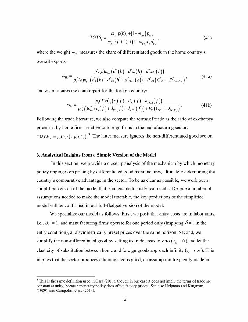
12

TOTSt

Ht

p(h)t 1

Ht pH ,t

Ft

etp*( f )

t 1

Ft etp*

F ,t

, (41)

where the weight Ht measures the share of differentiated goods in the home country’s

overall exports:

* * * *

,1

* * * * * * *, , ,1

( )

( )

t t Kt AC tt

Htt Kt AC t Ht Ht AC H tt t

p h n c h d h d h

p h n c h d h d h P C D

, (41a)

and Ft measures the counterpart for the foreign country:

*

1 ,

*1 , , ,

( )

( )t t t Kt AC t

Ftt t t Kt AC t Ft Ft AC F t

p f n c f d f d f

p f n c f d f d f P C D

. (41b)

Following the trade literature, we also compute the terms of trade as the ratio of ex-factory

prices set by home firms relative to foreign firms in the manufacturing sector:

*( ) / ( )t t t tT O T M p h e p f .3 The latter measure ignores the non-differentiated good sector.

3. Analytical Insights from a Simple Version of the Model

In this section, we provide a close up analysis of the mechanism by which monetary

policy impinges on pricing by differentiated good manufactures, ultimately determining the

country’s comparative advantage in the sector. To be as clear as possible, we work out a

simplified version of the model that is amenable to analytical results. Despite a number of

assumptions needed to make the model tractable, the key predictions of the simplified

model will be confirmed in our full-fledged version of the model.

We specialize our model as follows. First, we posit that entry costs are in labor units,

i.e., K = 1, and manufacturing firms operate for one period only (implying in the

entry condition), and symmetrically preset prices over the same horizon. Second, we

simplify the non-differentiated good by setting its trade costs to zero ( 0N ) and let the

elasticity of substitution between home and foreign goods approach infinity ( ). This

implies that the sector produces a homogeneous good, an assumption frequently made in

3 This is the same definition used in Ossa (2011), though in our case it does not imply the terms of trade are constant at unity, because monetary policy does affect factory prices. See also Helpman and Krugman (1989), and Campolmi et al. (2014).

1

13

the trade literature.4 Third, we restrict productivity shocks to be i.i.d., and only occur in the

differentiated good sector (we abstract from productivity shocks in the non-differentiated

good sector). Fourth, utility is log in consumption and linear in leisure ( 0 ). Finally,

drawing on the NOEM literature (see Corsetti and Pesenti 2005, and Bergin and Corsetti

2008), we carry out our analysis of stabilization policy by defining a country’s monetary

stance as PC , under the control of monetary authorities via their ability to set the

interest rate. Following this approach, we therefore study monetary policy in terms of

(and * for the foreign country), instead of the interest rate rule (33).

Under these assumptions---in particular, using the fact that the discount rate for

nominal quantities can be written as the (inverse of the) growth rate of ---the firms’

problem becomes

maxpt1 h

Et

t

t1

t1

h

.

The optimal preset price in the domestic market is:

11

1

111

tt t

t

tt t

WE

p hE

, (42)

where 1 1 1 1t t t tW is the firm’s marginal costs, that is, the ratio of nominal wages

to labor productivity. In this simplified model setting, the stochastically discounted value of

future demand facing the firm for its good in both markets, 1t , becomes:

*1 1 1 11t t t tc h c h .5

The home entry condition is a function of price setting and the exchange rate:

11 1 1

1

t tt t t t

t

KE p h p h

. (43)

4 Different from the trade literature, however, we do treat this sector as an integral part of the (general) equilibrium allocation, e.g., exports/imports of the homogeneous good sector enters the terms of trade of the country. 5 Upon appropriate substitutions and cancellations, equation (42) may also be written with 1t defined as

1 11 11 11 * * 1 1 * * 11 11 1 1 1 1 1 1 1 1( ) ( ) 1 ( ) ( ) 1t tt t t t t t t t tn p h n p f e n p h n p f e

.

t t tPC

14

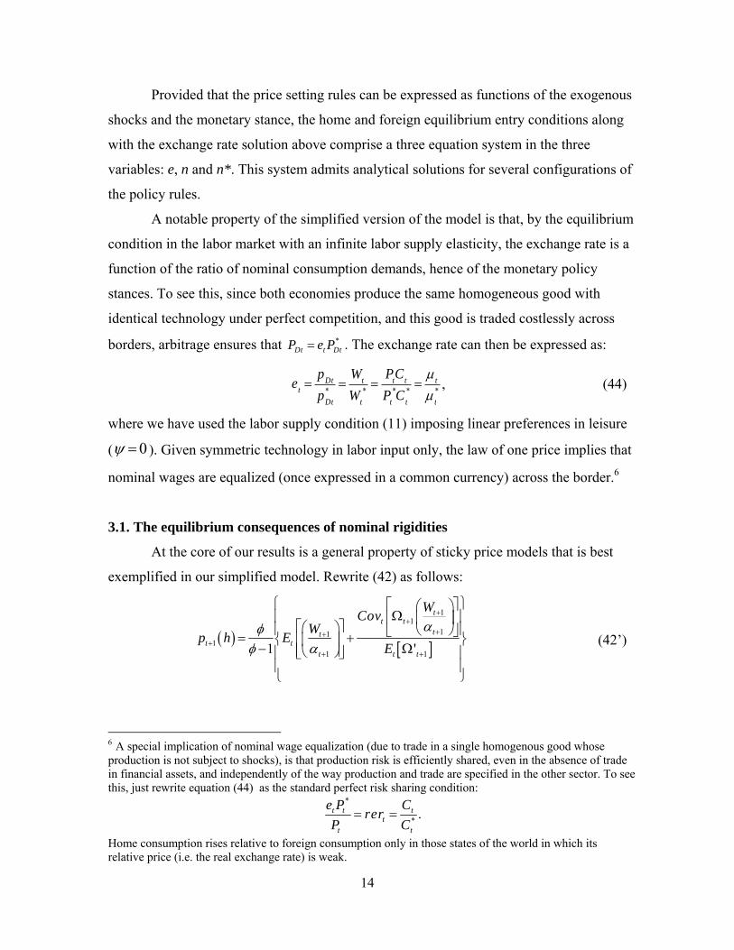
Provided that the price setting rules can be expressed as functions of the exogenous

shocks and the monetary stance, the home and foreign equilibrium entry conditions along

with the exchange rate solution above comprise a three equation system in the three

variables: e, n and n*. This system admits analytical solutions for several configurations of

the policy rules.

A notable property of the simplified version of the model is that, by the equilibrium

condition in the labor market with an infinite labor supply elasticity, the exchange rate is a

function of the ratio of nominal consumption demands, hence of the monetary policy

stances. To see this, since both economies produce the same homogeneous good with

identical technology under perfect competition, and this good is traded costlessly across

borders, arbitrage ensures that *Dt t DtP e P . The exchange rate can then be expressed as:

et

pDt

pDt*

Wt

Wt*

PtC

t

Pt*C

t*

t

t*, (44)

where we have used the labor supply condition (11) imposing linear preferences in leisure

( 0 ). Given symmetric technology in labor input only, the law of one price implies that

nominal wages are equalized (once expressed in a common currency) across the border.6

3.1. The equilibrium consequences of nominal rigidities

At the core of our results is a general property of sticky price models that is best

exemplified in our simplified model. Rewrite (42) as follows:

11

111

1 11 '

tt t

ttt t

t t t

WCov

Wp h E

E

(42’)

6 A special implication of nominal wage equalization (due to trade in a single homogenous good whose production is not subject to shocks), is that production risk is efficiently shared, even in the absence of trade in financial assets, and independently of the way production and trade are specified in the other sector. To see this, just rewrite equation (44) as the standard perfect risk sharing condition:

*

*.t t t

tt t

e P Crer

P C

Home consumption rises relative to foreign consumption only in those states of the world in which its relative price (i.e. the real exchange rate) is weak.

15

By the covariance term on the right-hand side of this expression, the optimal preset price is

a function of the comovements of a firm’s marginal costs ( 1 1 1 1t t t tW ), and overall

(domestic and foreign) demand for the firm’s good, 1t . To appreciate the relevance of

this property for the monetary transmission mechanism, consider the extreme case of no

monetary stabilization of business cycle fluctuation, i.e., posit that the monetary stance

does not respond to any shock, but target a constant nominal demand in either country

( * 1t t ). This implies a constant nominal exchange rate at */ 1t t te and, with i.i.d.

shocks, no dynamics in predetermined variables such as prices and numbers of firms.

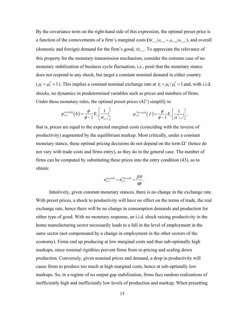
Under these monetary rules, the optimal preset prices (42’) simplify to

11

1

1no stabt t

t

p h E

*1 *

1

1

1no stab

t tt

p f E

,

that is, prices are equal to the expected marginal costs (coinciding with the inverse of

productivity) augmented by the equilibrium markup. Most critically, under a constant

monetary stance, these optimal pricing decisions do not depend on the term Ω’ (hence do

not vary with trade costs and firms entry), as they do in the general case. The number of

firms can be computed by substituting these prices into the entry condition (43), so to

obtain:

*1 1

no stab no stabt tn n

q

.

Intuitively, given constant monetary stances, there is no change in the exchange rate.

With preset prices, a shock to productivity will have no effect on the terms of trade, the real

exchange rate, hence there will be no change in consumption demands and production for

either type of good. With no monetary response, an i.i.d. shock raising productivity in the

home manufacturing sector necessarily leads to a fall in the level of employment in the

same sector (not compensated by a change in employment in the other sectors of the

economy). Firms end up producing at low marginal costs and thus sub-optimally high

markups, since nominal rigidities prevent firms from re-pricing and scaling down

production. Conversely, given nominal prices and demand, a drop in productivity will

cause firms to produce too much at high marginal costs, hence at sub-optimally low

markups. So, in a regime of no output gap stabilization, firms face random realizations of

inefficiently high and inefficiently low levels of production and markup. When presetting

16

prices, managers maximize the value of their firm by trading off higher markups in the low

productivity state, with lower markups in the high productivity states. In our model above,

they weigh more the risk of producing too much at high marginal costs: it is easy to see that

preset prices are increasing in the variance of productivity shocks (by Jensen’s inequality,

Et

1

t1

1

Et

t1

1).7

Since both marginal costs and overall demand are functions of monetary stances, in

the general case policy regimes can critically impinge on pricing (and thus on entry) via the

covariance term in the equation. The implications for our argument are detailed next.

3.2. Prices and firm dynamics under efficient and inefficient stabilization of output

gaps

Suppose that the monetary stance in each country moves in proportion to

productivity in the differentiated good sector: t

t,

t*

t* . The exchange rate in this

case is not constant, but contingent on productivity differentials, so that the home currency

systematically depreciates in response to an asymmetric rise in home productivity:

*t

tt

e

.

It is easy to see that, by ensuring that the nominal marginal costs μ/α remain constant, the

above policy zeroes the covariance term in (see (42’)), and thus insulates the ex-post

markup charged by home manufacturing firms from uncertainty about productivity.8 Note

that, to the extent that monetary policy stabilizes marginal costs completely, it also

stabilizes markups at their flex-price equilibrium level. It follows that the price firms

preset is lower than in an economy with no stabilization:

7 As discussed in Corsetti and Pesenti (2005) and Bergin and Corsetti (2008) in a closed economy context, given nominal demand, high preset prices allow firms to contain overproduction when low productivity squeezes markups, rebalancing demand across states of nature. High average markups, in turn, exacerbate monopolistic distortions and tend to reduce demand, production and employment on average, discouraging entry. 8 As is well understood, the policy works as follows: in response to an incipient fall in domestic marginal costs domestic demand and a real depreciation boost foreign demand for domestic product. As nominal wages rise with aggregate demand, marginal costs are completely stabilized at a higher level of production. Vice versa, by curbing domestic demand and appreciating the currency when marginal costs are rising, monetary policy can prevent overheating, driving down demand and nominal wages. Again, marginal costs are completely stabilized as a result.

17

1 11

1

1 1stab no stabt t t

t

p h p h E

.

In a multi-sector context, a key effect of monetary stabilization is that of reducing a

country’s differentiated goods’ price in terms of domestic nondifferentiated goods,

redirecting demand across sectors. This rise in demand for differentiated goods supports

the entry of additional manufacturing firms.

Since the model posits that the homogenous good sector operates under perfect

competition and flexible prices, there is no trade-off in stabilizing output across different

sectors. It is therefore possible to replicate the flex-price allocation under a monetary

policy rule that stabilizes markups in the differentiated sector. As shown in the appendix,

under this rule the number of manufacturing firms is:9

nt1stab

qE

t

2

t1

*t

1

1 1 1 1

1 1

1

t1

*t

1

1 1 1 1

1 1

t1

*t1

2(1 )

the same as under flexible prices.10

Consider instead the case in which, while the home government keeps stabilizing its

output gap, the foreign country switches monetary regime to a currency peg:

* and 1, so that t t t t t te .11

Under the policy scenario just described, the optimally preset prices of domestically and

foreign produced differentiated goods are, respectively:

1 1tp h

, * 11 *

11t

t tt

p f E

.

9 As discussed in the appendix, it is not possible to determine analytically whether symmetric stabilization policies raise the number of firms compared to the no stabilization case. Model simulations suggest that there is no positive effect for log utility, and a small positive effect for CES utility with a higher elasticity of substitution. Nonetheless, we are able to provide below an analytical demonstration of asymmetric stabilization, which is our main objective. 10 The above generalizes to our setup a familiar result of the classical NOEM literature (without entry) assuming that prices are sticky in the currency of the producers (Corsetti and Pesenti (2001, 2005) and Devereux and Engel (2003), among others): despite nominal rigidities, policymakers are able to stabilize the output gap relative to the natural-rate, flex-price allocation. 11 A related exercise consists of assuming that the foreign country keeps its money growth constant

( * 1t ) while home carries out its stabilization policy as above.

18

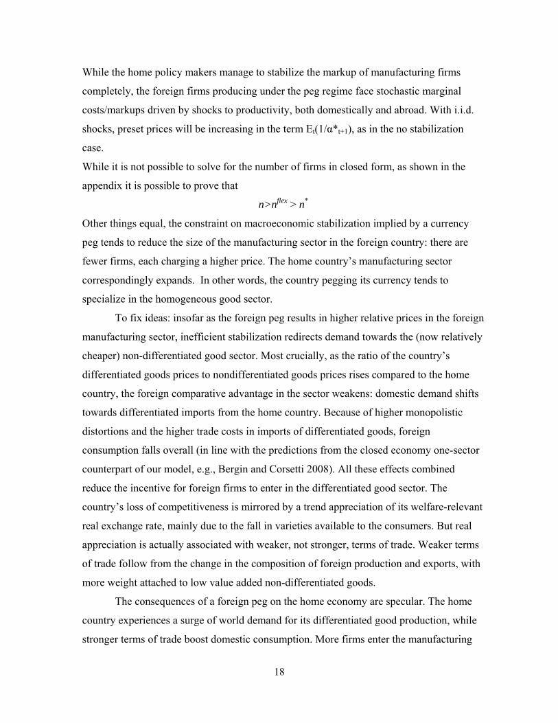
While the home policy makers manage to stabilize the markup of manufacturing firms

completely, the foreign firms producing under the peg regime face stochastic marginal

costs/markups driven by shocks to productivity, both domestically and abroad. With i.i.d.

shocks, preset prices will be increasing in the term Et(1/α*t+1), as in the no stabilization

case.

While it is not possible to solve for the number of firms in closed form, as shown in the

appendix it is possible to prove that

n>nflex > n*

Other things equal, the constraint on macroeconomic stabilization implied by a currency

peg tends to reduce the size of the manufacturing sector in the foreign country: there are

fewer firms, each charging a higher price. The home country’s manufacturing sector

correspondingly expands. In other words, the country pegging its currency tends to

specialize in the homogeneous good sector.

To fix ideas: insofar as the foreign peg results in higher relative prices in the foreign

manufacturing sector, inefficient stabilization redirects demand towards the (now relatively

cheaper) non-differentiated good sector. Most crucially, as the ratio of the country’s

differentiated goods prices to nondifferentiated goods prices rises compared to the home

country, the foreign comparative advantage in the sector weakens: domestic demand shifts

towards differentiated imports from the home country. Because of higher monopolistic

distortions and the higher trade costs in imports of differentiated goods, foreign

consumption falls overall (in line with the predictions from the closed economy one-sector

counterpart of our model, e.g., Bergin and Corsetti 2008). All these effects combined

reduce the incentive for foreign firms to enter in the differentiated good sector. The

country’s loss of competitiveness is mirrored by a trend appreciation of its welfare-relevant

real exchange rate, mainly due to the fall in varieties available to the consumers. But real

appreciation is actually associated with weaker, not stronger, terms of trade. Weaker terms

of trade follow from the change in the composition of foreign production and exports, with

more weight attached to low value added non-differentiated goods.

The consequences of a foreign peg on the home economy are specular. The home

country experiences a surge of world demand for its differentiated good production, while

stronger terms of trade boost domestic consumption. More firms enter the manufacturing

19

sector, leading to a shift in the composition of its production and exports in favor of this

sector.

As a result, with a foreign country passively pegging its currency, there are extra

benefits for the home country from being able to pursue stabilization policies. The home

manufacturing sector expands driven by higher home demand overall, and fills part of the

gap in manufacturing production no longer supplied by foreign firms. At the same time, the

shifting pattern of specialization ensures that the home demand for the homogeneous good

is satisfied via additional imports from the foreign country.

4. Numerical simulations

In this section, we evaluate the quantitative implications of our full model, by

conducting stochastic simulations. Despite the many differences between the simplified and

the full version of our model, we will show that the key results from the former continue to

hold in the latter. Namely, in our general specification it will still be true that, if the foreign

country moves from efficient stabilization to a peg, while the home country sticks to

efficient stabilization rules, (a) the foreign average markups and prices in manufacturing

will tend to increase and (b) there will be production relocation---firm entry in the foreign

country will fall on average, while entry in the home country will rise on average.

Correspondingly, average consumption will rise at home relative to foreign. We will also

show that this relocation will be associated with an average improvement in the home

terms of trade (while the home welfare-relevant real exchange rate depreciates).

To illustrate the core properties of the model, we initially assume that productivity

shocks are the only source of uncertainty, and discuss their effects in a number of variants

of the model relative to our baseline specification. After showing the impulse responses

generated by fluctuations in manufacturing productivity, we will discuss the effect of

productivity uncertainty on the unconditional means of macroeconomic variables, drawing

from stochastic simulations of a second order approximation of the model. In a final

subsection, we include in the model additional sources of uncertainty, considering a

number of shocks studied in the literature. Throughout our experiments, we contrast two

policy scenarios: symmetric output stabilization policies versus asymmetric stabilization,

20

with the foreign country authorities pegging to the home country. We start with our

calibration of the model, discussed next.

4.1. Parameter values

Parameter values are chosen to be consistent with an annual frequency---the

frequency at which sectoral productivity data are available. We set time preferences at

0.96 ; risk aversion at the standard value of 2 ; labor supply elasticity at 1/ 1.9

following Hall (2009), though we will check for sensitivity of our results to this

parameter.

The price stickiness parameter is set at p 8.7 , a modest value which in a Calvo

setting would correspond to half of firms resetting price on impact of a shock, with 75

percent resetting their price after one year.12 The death rate is set at 0.1 , which is four

times the standard rate of 0.025 to reflect the annual frequency. The sunk cost of entry is

normalized to the value 1.

To choose parameters for the differentiated and non-differentiated sectors we draw

on Rauch (1999). We choose so that differentiated goods represent 57 percent of U.S.

trade in value.13 The home share of non-differentiated goods is set at 0.5 , which implies

a trade share of about 30%, given the trade costs and elasticities below. To set the

elasticities of substitution for the differentiated and non-differentiated goods we draw on

the estimates by Broda and Weinstein (2006), classified by sectors based on Rauch (1999).

The Broda and Weinstein (2006) estimate of the elasticity of substitution between

12 As is well understood, a log-linearized Calvo price-setting model implies stochastic difference equation

for inflation of the form 1t t t tE mc , where mc is the firm’s real marginal cost of production, and

where 1 1 /q q q , with q is the constant probability that firm must keep its price unchanged in any

given period. The Rotemberg adjustment cost model used here gives a similar log-linearized difference equation for inflation, but with 1 / . Under our parameterization, a Calvo probability of q = 0.5

implies an adjustment cost parameter of 8.7 . This computation is confirmed by a stochastic simulation of a permanent shock raising home differentiated goods productivity without international spillovers, which implies that price adjusts 50% of the way to its long run value immediately on impact of the shock, and 75% at one period (year in our case) after the shock. 13 Values vary by year and by whether a conservative or liberal aggregation is used. Taking an average over the three sample years and the two aggregation methods reported in Table 2 of Rauch (1999) produces an average of 0.57. Replicating this value in our steady state requires a calibration of the consumption share at =0.38, which compensates for the fact that trade for investment purposes (sunk cost) involves differentiated goods only.

21

differentiated goods varieties is =5.2 (the sample period is 1972-1988). The

corresponding elasticity of substitution for nondifferentiated commodities is = 15.3.

To set trade costs, we need to think beyond costs associated with just transportation.

These are often thought to be higher for commodities than for high-value differentiated

goods. As Rauch (1999) points out, differentiated goods involve search and matching costs,

whereas commodities and goods traded on an organized exchange with a published

reference price avoid such costs. Estimates are available for the tariff equivalent of

language costs, with a value of 11% in Hummels (1999) or 6% in Anderson and van

Wincoop (2004), so we use 8% in between. Since Obstfeld and Rogoff (2000) recommend

a calibration of total trade costs at 16%, our calibration implies that half of this is due to

language and matching costs, and the other half due to transportation. This implies a

calibration of D = 0.16 for differentiated goods, and N =0.08 for non-differentiated goods.

The parameters in the home monetary policy rule are determined by the values that

maximize home utility. As typically found, the optimal weight on inflation is the maximum

value considered in the grid search ( P =1000), and the optimal value on output is Y =0.

The foreign country is assumed to peg its exchange rate at parity with the home country:

e=1. To our knowledge, no one else has calibrated a DSGE model with sectoral shocks

distinct to differentiated and nondifferentiated goods. Annual time series of sectoral

productivities are available from the Groningen Growth and Development Centre (GGDC),

for the period 1980-2007. Data for the U.S. is used to parameterize shocks to the home

country, and an aggregate of the EU 10 for the foreign country.14 TFP is calculated on a

value-added basis. For each country, the differentiated goods sector comprises total

manufacturing excluding wood, chemical, minerals, and basic metals; the non-

differentiated goods sector comprises agriculture, mining, and subcategories of

manufacturing excluded from the differentiated sector. To calculate the weight of each

subsector within the differentiated (or non-differentiated) sector, we use the 1995 gross

value added (at current prices) of each subsector divided by the total value added for the

differentiated (or non-differentiated) sector. After taking logs of the weighted series, we de-

14 These EU 10 countries are AUT, BEL, DNK, ESP, FIN, FRA, GER, ITA, NLD and the UK. See http://www.euklems.net/euk08i.shtml.

22

trend each series using the HP filter. Parameters and Ω, reported in Table 1, are obtained

from running a VAR(1) on the four de-trended series.

The benchmark simulation model specifies entry costs in units of goods ( K =0) but

we will also report results for entry costs in labor units in our sensitivity analysis (see the

discussion in Cavallari 2013). The adjustment cost parameter for new firm entry, , is

chosen to match the standard deviation of new firm entry in the benchmark simulation to

that in data. The World Bank’s Entrepreneurship Survey and data base provides a count of

new businesses registered during a calendar year, for the period 2004 to 2012 for selected

countries. We use the data available for France, Germany, Italy and the U.K. to represent

the foreign country in our model. Data for the U.S. on establishment entry are available

from the Longitudinal Business Database. Standard deviations for logged and HP-filtered

series are reported as ratios to the standard deviation of GDP for the same period: the value

for the U.S. is 5.53, and the European average is 3.01. A value of = 0.25 in the

simulation model, with the remaining parameters and shocks as described above, generates

standard deviations of new firm entry close to these values. (See Table 2b.)

4.2. Simulation results

4.2.1. Impulse responses

Figure 1 reports the dynamics of the benchmark model in response to a one

standard deviation positive shock to productivity in the differentiated goods sector of the

home country, where both countries employ efficient stabilization policy. The figure plots

the percentage deviation from the unconditional mean of key variables of interest. As

home policymakers fully stabilize the markup, they react to the shock by expanding

domestic demand and depreciating the exchange rate. This policy reaction boosts

production in the differentiated sector, in line with its enhanced productivity. The number

of firms in the sector rises, and production shifts in favor of home differentiated goods,

away from nondifferentiated goods. In the foreign country, the shift in production pattern

partly reflects the cross-country autocorrelation of shocks in the calibration. Since the

foreign country also experiences a rise in differentiated goods productivity, the number of

firms and the volume of differentiated output also rise in this country, though by a smaller

magnitude than at home where the shock originated, and with a one period lag.

23

To further clarify the role of the cross-country correlation of shocks, in Figure 2 we

redo the analysis by setting the cross-country elements of the shock autorcorrelation matrix

equal to zero. This figure thus shows the effects of a rise in the differentiated goods

productivity at home that remains asymmetric. Foreign production of differentiated goods

falls (while it rises at home); conversely foreign production of nondifferentiated goods rises

(while it falls at home).

The case of asymmetric policies---with the foreign country pegging its exchange

rate, and the home country employing efficient stabilization policy---is shown in the next

two figures. In response to a favorable shock to home differentiated-goods productivity, the

behavior of home variables in Figure 3 is very similar to Figure 1. But in Figure 3, the

response of the foreign variables closely resembles those of the home variables. The

commitment to exchange rate stability causes the foreign monetary authorities to expand

money supply and demand by more, in step with the home country, providing extra

stimulus to the foreign differentiated goods sector at the expense of the nondifferentiated

goods sector.

Figure 4 shows the effects of a productivity shock to the differentiated goods sector

in the country pursuing a peg (that is, foreign). It differs noticeably from the other figures.

In the absence of a stabilizing policy response, manufacturing entry in the foreign economy,

while positive, is an order of magnitude smaller compared to entry in the home economy in

the previous figures. Likewise, the rise in foreign production of differentiated goods is

much smaller and much shorter lived.

4.2.2. Unconditional means

Table 2a reports the unconditional means of key variables obtained from stochastic

simulations of a second order approximation of the benchmark model, and Table 2b reports

standard deviations. In Column (1) of Table 2a both countries use stabilization policy,

while in column (2) the foreign country adopts an exchange rate peg. Column (3) reports

the percent change between the previous columns, hence accounting for changes when the

foreign country pursues a peg instead of inflation stabilization. Note that country means in

column (1) are not completely symmetric despite symmetric policies, due to the cross-

border differences in the estimated TFP shock process.

24

The simulation results fully confirm the main analytical insights from the previous

section. When the foreign country pegs, average production of the differentiated good

shifts away from the foreign country and toward the home country; the foreign country

instead has higher production of the non-differentiated good. This shift in production is

reflected in a 0.73 percent fall in the number of foreign differentiated goods firms, in

contrast to a 0.63 percent rise at home: the ratio of foreign firms relative to the home

counterpart falls 1.36 percent. The share of differentiated goods in exports ( F ) falls by

0.56 percent in the foreign country, while the share in the home country ( H ) rises by 0.61

percent. This implies that the ratio of the foreign export share relative to the home

counterpart falls 1.17 percent.

Also consistent with the transmission mechanism discussed in the previous section,

what drives the foreign loss in the differentiated goods market share under a peg is the

higher average markup charged by foreign producers of these goods. Note that the foreign

price of differentiated goods rises relative to both wages and non-differentiated goods (.07

percent in both cases).

Finally, when the foreign policymaker abandons efficient stabilization policy for a

peg, the foreign terms of trade including the homogenous good, TOTS, actually worsen (.38

percent). This stands in contrast with the movements in the (conventionally-defined) terms

of trade including only differentiated goods, TOTM, which remains nearly unchanged (.01

percent). The different behavior of the TOTS and TOTM is due to a composition effect: the

shift in foreign export share away from differentiated goods means these more expensive

goods receive a smaller weight in the average price of foreign exports and a larger weight

in the average price of foreign imports.

International price adjustment highlights a notable difference between the

simplified and the full model. As our results in Table 2a emphasize, despite a lower markup,

the terms of trade of manufacturing do not necessarily fall with better stabilization. This

will be so because, in the full model, a high level of entry tends to raise production costs, as

on average wages respond to a higher demand for domestic labor. To the extent that labor

supply is not infinitely elastic (as assumed in the simplified model), this effect may become

strong enough to prevent the international price of domestic manufacturing from falling in

tandem with average markup in the sector.

25

Table 2b shows that the calibration of our model is in line with the volatility of

output in the US and the EU-10 countries, as well as the volatilities of key variables (in

ratio to the volatility of output), such as consumption, employment and net business

formation.

4.2.3. Alternative model specifications

Table 3 summarizes our results under alternative model specifications. To save

space, we only report the percentage change in number of firms and percent change in

differentiated export share when the foreign country switches from inflation stabilization to

exchange rate peg. The first column repeats for comparison the key result for the

benchmark case from Table 2a. This result depends completely upon free entry of firms:

Column (2) shows that the changes in differentiated export share disappear when the

number of firms is held fixed exogenously. The endogenous shift in number of firms

between countries is essential for the change in monetary policy to translate into

quantitatively meaningful effects on export shares.

The currency in which export prices are sticky, whether in units of the producer or

local currency, is not consequential to the effect of policy on product specialization. When

the price adjustment specification of the benchmark model is replaced by the local currency

version (the LCP version of Rotemberg pricing is detailed in the appendix) results are

nearly unchanged, as reported in column (3). Even if prices are inelastic to the exchange

rate in the short run, they are ex-ante sensitive to the covariance of marginal costs and

demand, which is the core mechanism by which monetary stabilization impinges on

competitiveness.

The result is also robust to relaxing the requirement that trade is balanced. The

appendix lists equations for a version of the model which includes international trade in

noncontingent bonds, which can be used to finance temporary current account imbalances

in response to shocks. Column (4) of the table shows that the effect of the peg on relative

firm entry and export share is similar to that under balanced trade, and even slightly

magnified.

This result is somewhat stronger, when we allow for stickiness in wages as well as

prices. In the version of the model simulated in column (5) of the table, we allow for

26

households to supply differentiated labor, indexed by j, and face a cost of adjusting wages

2

, 1 12

wW s s s sAC j W j W j l j

, whereas labor demand is L

t t t tl j W j W l

.

Utility maximization now implies the following wage setting condition:

21

1 1 1

1 11 1 2

1

11 1 2 1

2

11

t t w t t tL L t L

t t t t t

t tt t t w

t t t

l l W W Wl

W W W W

W WE W l

W W

to replace the optimal labor supply conditions (also, we amend the labor market clearing

condition to include the labor expended in adjusting the wage). Barattieri et al. (2014)

estimates the average time to reset a wage is between 3.8 and 4.7 quarters. To match this

finding we apply the logic employed above for the sticky price calibration, and compute

that a value of w = 32.3 in our annual model implies that half of wages have been reset one

year after a shock. The substitutability between labor varieties is set to L =6. The

parameterization of the monetary policy rule is adjusted to p = 3.15

Sticky wages significantly amplify the effect of a peg on the steady state number of

firms and export shares, lowering the foreign/home ratios by 3.7% and 2.9%, respectively

(see column 5). Some intuition can be draw from equation (42’) derived for the case of the

simplified model. Recall that differentiated goods prices are set lower, hence encouraging

greater specialization in differentiated goods, if there is a smaller covariance of nominal

marginal costs (wage divided by productivity) with demand. Firms dislike a situation where

they are required to produce more when production costs are high. In the benchmark

simulation with only price stickiness, monetary policy assures that demand is high during

positive productivity shocks that lower production costs. But this policy also has the effect

of raising nominal wages, which works the opposite direction to raise production costs.

15 No solution is possible in the model when significant wage rigidity is combined with a monetary policy that tries to hold prices nearly constant. Because prices depend primarily upon the production cost, that is, the ratio of wage to the productivity, a shock to productivity requires a similar movement in wage if prices are to remain constant. We resolve this problem by reducing the weight on inflation in the monetary policy rule, using a value of 3 based on Schmidt-Grohe and Uribe (2007).

27

Sticky wages work to prevent such a rise in wage costs, and hence maintain a low

covariance of costs with demand.16

Another key determinant of the rise in wages and hence costs following a shock is

the labor supply elasticity. Recall that the preferences assumed in the analytical model

imply an infinite labor supply elasticity, in contrast with the value of 1.9 assumed in the

numerical economy. There is a wide range of values for this elasticity supported in the

macroeconomics literature.17 When the labor supply elasticity is raised in the simulation

model to an extreme value of 5, we obtain a modest rise in effect of a peg on the mean

export share (see column 6).

However, the effect becomes much stronger when a high labor supply elasticity is

combined with a change in the specification of preferences to remove the wealth effect on

labor supply, as in a GHH specification. In the version of the model simulated in column

(7), we replace our baseline preference specification with the following:

11 1 1 lnt t t t tU C l M P

, which implies that labor is optimally supplied

according to t t tl W P and 1 1t t t tP C l .

The effect of a peg on the number of firms and the differentiated export share is

amplified by an order of magnitude compared to the benchmark model, as seen in column

(7). The mechanism is similar to that for the sticky wage case. The preference specification

removes the wealth effect in wage determination, in that consumption does not appear in

the labor supply condition. Unlike the benchmark model, a rise in consumption induced by

a rise in productivity does not require a rise in wage to induce workers to supply labor.

Hence there is less pressure for wage costs to rise with production, which in turn lowers the

covariance between costs and output.18

In column (8), we adopt the version of the model in column 7 but redefine entry

costs in labor units only ( K =1)---the same specification used in the simplified model of

16 Implications of policy for the mean level of sticky wages have little impact on comparative advantage in our model, since, in contrast with sticky prices, the wage rate affects both sectors symmetrically. 17 See for Example Keane and Rogerson (2012). 18 We also investigated a version of the model with complementarity between consumption and labor, as advocated in Hall and Milgrom (2008). While this specification did dampen the rise in wage during a rise in output and hence raise the mean share of differentiated goods in exports, the effect was small, and this case is not reported in our table of results.

28

section 3. The effect of stabilization policy on the mean level of wages has strong

implications for the mean level of entry. Recall from the benchmark case in Table (2a) that

a stabilizing country has a higher mean wage compared to the pegging country. When entry

cost is specified in labor units, this effect can strongly dampen entry, as it moves against

the benefits of output stabilization on firms’ value. Indeed, results in column (8) are smaller

than in the benchmark

Another feature of the benchmark model that could limit the effect of a peg is the

correlation of exogenous shocks across countries. The fairly high shock correlations in the

benchmark calibration reflect the close relationship between the U.S. and the EU-10

countries in the data used for calibration. But this high correlation might not apply to other

countries. Column (9) of Table 3 shows that if the calibration assumes zero

contemporaneous correlations across all shocks, the effect of the peg on entry and export

shares doubles compared to the benchmark calibration.

4.2.4. Alternative shocks

To gain further insight into the monetary transmission mechanism that is relevant

for our results, we now consider the model including additional sources of uncertainty.

Drawing on the literature we include a shock to money demand, consumption demand, and

taxes. We include the first two shocks by augmenting the utility function with terms to shift

the marginal utility of money balances ( ) and consumption ( ):

1 11 1ln

1 1t

t t t t tt

MU C l

P

.

To consider a tax shock, let DtT represent the fraction of differentiated good production that

is surrendered to the government, so that the differentiated goods market clearing condition

becomes: *1 1Dt t D tT y h d h d h . Similarly for a tax on nondifferentiated

goods production, N tT , market clearing becomes

* *, , , , , , ,1 1Nt H t H t AC H t N H t AC H tT y C D C D . It is assumed that the goods surrendered

to the government as tax payments are consumed directly by the government, and this

yields no household utility. This implies pricing equations for the two types of goods:

29

2 2

1 1 1

2

1 11

1

11 1

1 1 2 1

11

t t tt Pt t P

t Dt t t t

t tt tPt

t t t t

p h p h p hWp h p h

T p h p h p h

p h p hE

p h p h

and ,

, 1t

H tH t Nt

Wp

T

.

Note from these equations that from the firm’s perspective this tax shock is very similar to

a negative productivity shock. In addition, noting the way the shock enters the price setting

function, it also is isomorphic to the markup shock studied in Corsetti et al. (2010).

All shocks are assumed to follow autoregressive processes in log deviations from

steady state, orthogonal to other shocks, and orthogonal across countries. The

parameterization of the tax shock is taken from the estimations of Leeper et al. (2010).19

Parameterization of the consumption taste shock is taken from Stockman and Tesar (1995),

and that of the money demand shock is taken from Bergin et. al (2007). 20

Results are reported in Table 4. As a benchmark, we first show that shocks to

money demand are not relevant: under the monetary regimes considered in either of our

experiments, any rise in money demand is automatically matched by a rise in supply---this

is true both under full output gap stabilization and under a peg. Simulations confirm that

the mean number of firms or differentiated export share, shown in Column (1), is

unaffected, and so are the other variables in the model. This type of shock could be

potentially consequential for firms’ entry only under monetary regimes, such as a constant

money growth rule, that would fall short of insulating aggregate demand from destabilizing

liquidity shocks, inducing a positive covariance between demand and marginal costs.

Also the shocks to consumption tastes (column 2) have little or no effect on the

entry into the differentiated goods sector. In contrast with money demand shocks, however,

19 The process estimated by Leeper et al (2010) for capital tax shocks is converted from a quarterly frequency to an annual frequency by stochastic simulation of the process and then fitting an annual sampling of the artificial data to a first order autoregression. The resulting autoregressive parameter of 0.741 and standard deviation of shocks of 0.0790 are applied to tax shocks in each country and each sector. These shocks are assumed to be orthogonal to each other. The mean level of this tax, 0.184, is also taken from Leeper et al (2010). 20 We follow the first experiment of Stockman and Tesar (1995), in parameterizing a shock to overall consumption with standard deviation 2.5 times that of productivity, and with the same autoregressive parameter as productivity. We follow Bergin et al (2007) in setting the standard deviation of the money demand shock at 0.030, with a serial corrleation of 0.99.

30

taste shocks do lead to fluctuation in the values of endogenous variables under our policy

rules. A policy of price level stabilization is not necessarily optimal in this case: if

monetary authorities optimize over the trade-offs between output gap and inflation, the

effects on entry could be somewhat larger. Yet the main lesson from our exercise would be

confirmed: as long as uncertainty does not impinge on the covariance between demand and

marginal costs, our main mechanism is not active.

Results are quite different in the case of the tax shock (column 3). In the context of

the tax shock in isolation, stabilization policy raises the unconditional mean of firm entry

by 90% of that under productivity shocks, and it raises the differentiated export share by 75%

of that under productivity shocks. Indeed, output gap stabilization affects the unconditional

mean of firm entry much like in the case of a productivity shock. Numerically, results are

actually similar to the case in which productivity shocks are anticipated, i.e., they are

“news shocks” a la Jaimovich and Rebelo (2009) (not reported in the table). With “news

shocks,” the entry effects are attenuated by the fact that forward looking firms start to

adjust prices in anticipation of shocks due to materialize in the future.

We conclude with an experiment combining all four shocks, shown in the last

column of the table. The overall effect of stabilization policy on firm entry and export

shares are by and large the sum of the effects under tax shocks and productivity shocks,

representing a significant magnitude.

5. Conclusion

According to a widespread view in policy and academic circles, monetary and

exchange rate policy has the power to benefit or hinder the competitiveness of the domestic

manufacturing sector. This paper revisits the received wisdom on this issue, exploring a

new direction for open-economy monetary models and empirical research. Our argument is

that macroeconomic stabilization affects the comparative advantage of a country in

producing goods with the characteristics (high upfront investment, monopoly power and

nominal frictions) typical of manufacturing. A stabilization regime that reduces output gap

(and marginal cost) uncertainty can strengthen a country’s comparative advantage in the

production of these goods, beyond the short run.

31

To be clear, an efficient stabilization policy requires contingent expansion and

contractions in response to shocks affecting the output gap, which ex post foster but may

also reduce the international price competitiveness of a country. Our results however

suggest that monetary stabilization may affect the long-run comparative advantage of a

country in a way that is separate from the prescription of pro-competitive devaluations

familiar from traditional policy models. By the same token, our analysis provides a novel

important insight on the conclusions of recent New Keynesian models, that monetary

policy should trade off output gap stabilization with stronger terms of trade. In our model,

efficient stabilization makes differentiated good manufacturing more competitive, and this

results in a shift in the sectoral allocation of resources and composition of exports, in favor

of high-value added goods in exports. It is this shift that improves the country’s overall

terms of trade, even if the international price of domestic manufacturing falls. Overall, the

theory developed in this paper points to new promising directions for integrating trade and

macro models and brings the literature closer to addressing core concerns in the policy

debate.

32

References Anderson, James E. and Eric van Wincoop, 2004. “Trade Costs,” Journal of Economic Literature 42, 691-751. Barattieri, Alessandro, Susanto Basu, and Peter Gottschalk, 2014. "Some Evidence on the Importance of Sticky Wages," American Economic Journal: Macroeconomics 6, 70-101. Benigno, Gianluca and Pierpaolo Benigno, 2003. “Price Stability in Open Economies,” Review of Economic Studies 70, 743-764. Bergin, Paul R. and Giancarlo Corsetti, 2008. “The Extensive Margin and Monetary Policy,” Journal of Monetary Economics 55, 1222-1237. Bergin, Paul R. and Giancarlo Corsetti, 2014. “International Competitiveness and Monetary Policy,” U.C. Davis mimeo. http://old.econ.ucdavis.edu/faculty/bergin/research/Bergin-Corsetti-061114-gc.pdf Bergin, Paul R., Hyung-Cheol Shin, and Ivan Tchakarov, 2007. "Does Exchange Rate Variability Matter for Welfare? A Quantitative Investigation of Stabilization Policies," European Economic Review 51(4), 1041-1058. Bilbiie, Florin O., Fabio Ghironi, and Marc J. Melitz, 2008. “Monetary Policy and Business Cycles with Endogenous Entry and Product Variety,” in Acemoglu, D., K. S. Rogoff, and M. Woodford, eds., NBER Macroeconomics Annual 2007, University of Chicago Press, Chicago, 299-353. Bodenstein, M., C.J. Erceg, and L. Guerrieri, 2008. “Optimal Monetary Policy with Distinct Core and Headline Inflation Rates,” Journal of Monetary Economics 55, S18–S33. Broda, Christian and David E. Weinstein, 2006. “Globalization and the Gains from Variety,” The Quarterly Journal of Economics 121, 541-585. Campolmi, Alessia, Harald Fadinger, and Chiara Forlati, 2014. “Trade Policy: Home Market Effect Versus Terms-of-trade Externality,” Journal of International Economics, 93(1): 92-107. Canzoneri, Matthew B. Robert E. Cumby and Behzad Diba, 2005. “The Need for International Policy Coordination; What’s Old, What’s New, What’s Yet To Come?” Journal of International Economics 66, 363-384. Cavallari, Lilia, 2013. “Firms' Entry, Monetary Policy and the International Business Cycle,” Journal of International Economics 91, 263-274. Corsetti, Giancarlo, Luca Dedola, and Sylvain Leduc, 2010. “Optimal Monetary Policy in Open Economies,” Handbook of Monetary Economics, vol III, ed by B. Friedman and M. Woodford, 861-933.

33

Corsetti, Giancarlo, Philippe Martin and Paolo Pesenti, 2007. “Productivity, Terms of Trade and the `Home Market Effect',” Journal of International Economics 73(1), 99-127. Corsetti, Giancarlo, and Paolo Pesenti, 2001. “Welfare and Macroeconomic Interdependence,” Quarterly Journal of Economics 116, 421-446. Corsetti, Giancarlo, and Paolo Pesenti, 2005. “International Dimensions of Optimal Monetary Policy,” Journal of Monetary Economics 52(2), 281-305. Devereux, Mick and Charles Engel, 2003. “Monetary Policy in the Open Economy Revisited: Price Setting and Exchange Rate Flexibility,” Review of Economic Studies 70, 765-783. Feenstra, Robert C., Robert E. Lipisey, Haizan Deng, Alyson, C. Ma and Hengyong Mo, 2005. “World Trade Flows,” NBER Working Paper 11040. Fernández-Villaverde, Jesús, Pablo Guerrón-Quintana, Juan F. Rubio-Ramírez, and Martin Uribe, 2011. “Risk Matters: The Real Effects of Volatility Shocks,” American Economic Review 101, 2530–2561. Ghironi, Fabio and Marc J. Melitz, 2005. “International Trade and Macroeconomic Dynamics with Heterogeneous Firms,” The Quarterly Journal of Economics 120(3), 865-915. Hall, Robert E., 2009. “By How Much Does GDP Rise If the Government Buys More Output?” Brookings Papers on Economic Activity 2, 183–231. Hall, Robert E, and Paul R. Milgrom, 2008. “The Limited Influence of Unemployment on the Wage Bargain,” American Economic Review 98, 1653-1674. Helpman, Elhanan and Paul Krugman, 1989. Trade Policy and Market Structure, MIT Press. Hummels, David, 1999. “Have International Transportation Costs Declined?” Work Paper, Purdue University. Jaimovich, Nir and Sergio Rebelo, 2009. “Can News about the Future Drive the Business Cycle?” The American Economic Review 99, 1097-1118. Leeper, Eric M., Michael Plante, and Nora Taum, 2010. “Dynamics of Fiscal Financing in the United States,” Journal of Econometrics 156, 304-321. Keane, Michael and Richard Rogerson, 2012. “Micro and Macro Labor Supply Elasticities: A Reassessment of Conventional Wisdom,” Journal of Economic Literature, 464-476. Krugman , Paul, 1980. “Scale Economies, Product Differentiation, and the Pattern of Trade,” American Economic Review 70, 950-959. Obstfeld, Maurice and Kenneth Rogoff, 2000. “New Directions for Stochastic Open Economy Models,” Journal of International Economics 50, 117-154.

34

Ossa, Ralph, 2011. “A “New Trade” Theory of GATT/WTO Negotiations,” Journal of Political Economy 119, 122-152. Rauch, James E., 1999. “Networks Versus Markets in International Trade,” Journal of International Economics 48, 7–35. Reinhart, Carmen, 2010. “This Time is Different Chartbook: Country Histories on Debt, Default, and Financial Crisis,” NBER Working Paper 15815. Reinhart, Carmen M. and Rogoff, Kenneth S., 2013. "Banking Crises: An Equal Opportunity Menace," Journal of Banking and Finance 37(11), 4557-4573. Schmitt-Grohe, Stephanie and Martin Uribe, 2007. "Optimal Simple and Implementable Monetary and Fiscal Rules," Journal of Monetary Economics 54, 1702-1725. Stockman, Alan C. and Linda Tesar, 1995. "Tastes and Technology in a Two-Country Model of the Business Cycle: Explaining International Comovements," American Economic Review 85(1), 168-85.

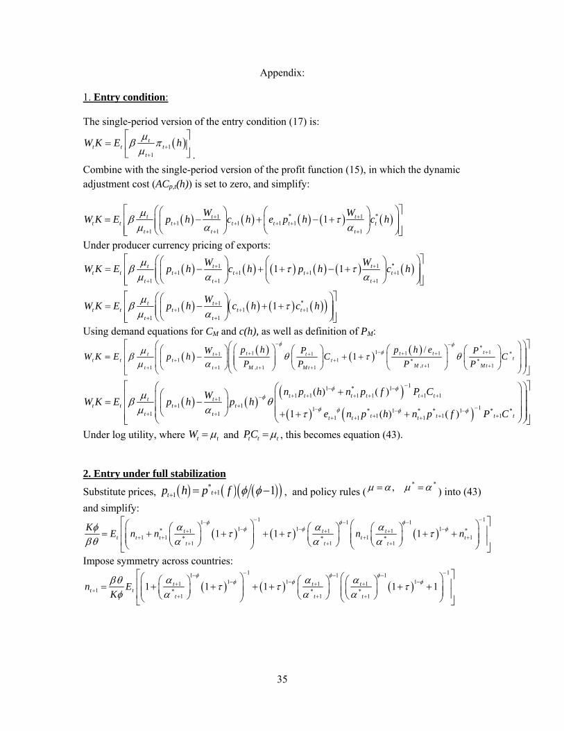
35

Appendix: 1. Entry condition: The single-period version of the entry condition (17) is:

11

tt t t

t

W K E h

. Combine with the single-period version of the profit function (15), in which the dynamic adjustment cost (ACp,t(h)) is set to zero, and simplify:

* *1 11 1 1 1

1 1 1

1t t tt t t t t t t

t t t

W WW K E p h c h e p h c h

Under producer currency pricing of exports:

*1 11 1 1 1

1 1 1

*11 1 1

1 1

1 1

1

t t tt t t t t t

t t t

t tt t t t t

t t

W WW K E p h c h p h c h

WW K E p h c h c h

Using demand equations for CM and c(h), as well as definition of PM:

*1 11 1 1 *1 1

1 1 * *, 1 11 1 , 1 1

/1

tt t tt t ttt t t t

M t M tt t M t M t

p h p h eW P PW K E p h C C

P P P P

11 * 11 1 1 1 1 1

11 1 11 * 1 * * 1 * *1 1 1 1 11 1 1

( ) ( )

1 ( ) ( )

t t t t t tt t

t t t tt t t t t tt t t

n p h n p f P CWW K E p h p h

e n p h n p f P C

Under log utility, where t tW and t t tPC , this becomes equation (43). 2. Entry under full stabilization

Substitute prices, *11 1ttp h p f , and policy rules (

* *, ) into (43)

and simplify:

1 11 1 1

1 1 1* *1 1 11 1 1 1* * *

1 1 1

1 1 1t t tt t t t t

t t t

KE n n n n

Impose symmetry across countries:

1 11 1 1

1 1 11 1 11 * * *

1 1 1

1 1 1 1 1t t tt t

t t t

n EK

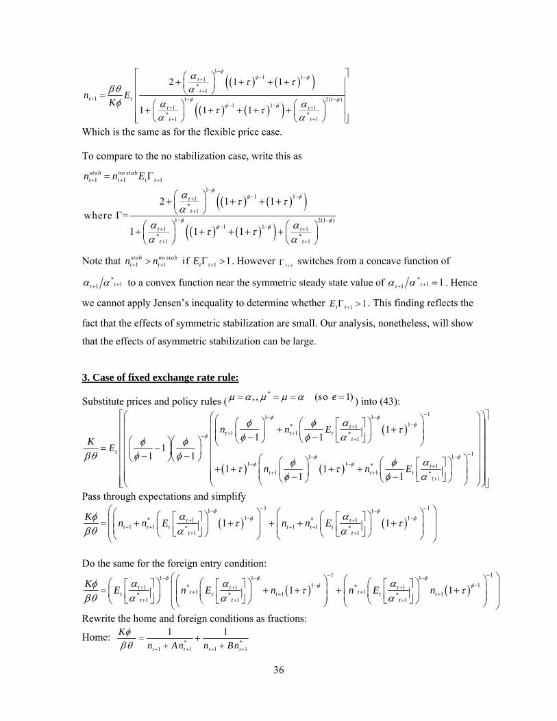
36

11 11

*1

1 1 2(1 )1 11 1

* *1 1

2 1 1

1 1 1

t

tt t

t t

t t

n EK

Which is the same as for the flexible price case. To compare to the no stabilization case, write this as

1 1 1

11 11

*1

1 2(1 )1 11 1

* *1 1

2 1 1where =

1 1 1

stab no stabt t t t

t

t

t t

t t

n n E

Note that 1 1 1 if 1stab no stabt t t tn n E . However

1t switches from a concave function of

*11 tt to a convex function near the symmetric steady state value of *

11 1tt . Hence

we cannot apply Jensen’s inequality to determine whether 1 1t tE . This finding reflects the

fact that the effects of symmetric stabilization are small. Our analysis, nonetheless, will show

that the effects of asymmetric stabilization can be large.

3. Case of fixed exchange rate rule:

Substitute prices and policy rules (*

*, (so 1)e ) into (43):

1111* 1

1 1 *1

1111 1 * 1

1 1 *1

11 1

11 1

1 11 1

tt t t

t

t

tt t t

t

n n EK

E

n n E

Pass through expectations and simplify

1 11 1

1 1* *1 11 1 1 1* *

1 1

1 1t tt t t t t t

t t

Kn n E n n E

Do the same for the foreign entry condition:

1 11 1 1

1 1* *1 1 11 11 1* * *

1 1 1

1 1t t tt tt t t t t

t t t

KE n E n n E n

Rewrite the home and foreign conditions as fractions:

Home: * *

1 1 1 1

1 1

t t t t

K

n An n Bn

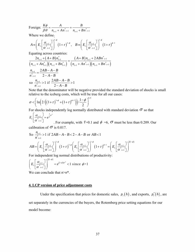
37

Foreign: * *

1 11 1t tt t

K A B

n An n Bn

Where we define:

Equating across countries:

Note that the denominator will be negative provided the standard deviation of shocks is small relative to the iceberg costs, which will be true for all our cases:

0.5

1 1 1ln 2/ 1 1 /

2

For shocks independently log normally distributed with standard deviation so that

. For example, with =0.1 and =6, must be less than 0.209. Our

calibration of is 0.017.

1*

1

So 1 if 2 2 or 1t

t

nAB A B A B AB

n

For independent log normal distributions of productivity:

We can conclude that n>n*. 4. LCP version of price adjustment costs

Under the specification that prices for domestic sales, tp h , and exports, *tp h , are

set separately in the currencies of the buyers, the Rotemberg price setting equations for our

model become:

1 1

1 11 1* *

1 1

1 , 1t tt t

t t

A E B E

* *11 1 1

* * * *1 11 1 1 1 1 1

2 2 tt t t

t tt t t t t t

n A B n A B n ABn

n An n Bn n An n Bn

1*

1

2

2t

t

n AB A B

n A B

1*

1

2so 1 if 1

2t

t

n AB A B

n A B

211 2

*1

tt

t

E e

1 1 2 1

1 11 1 1* * *

1 1 1

1 1t t tt t t

t t t

AB E E E

2

2 1

11*

1

1 since >1tt

t

E e

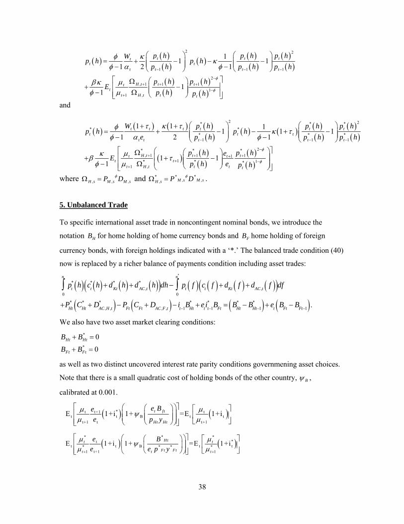
38

2 2

1 1 1

2

, 1 1 1

11 ,

11 1

1 2 1

11

t t ttt t

t t t t

H t t ttt

t H t t t

p h p h p hWp h p h

p h p h p h

p h p hE

p h p h

and

2 2* * ** *

* * *1 1 1

2* * *, 1 1 11

1 1* * *1 ,

1 1 11 1 1

1 2 1

1 11

t t t t t tt t t

t t t t t

H t t tt tt t

t H t t t t

W p h p h p hp h p h

e p h p h p h

p h p heE

p h e p h

where , , ,H s M s M sP D and * * *, ,, M s M sH s P D .

5. Unbalanced Trade To specific international asset trade in noncontingent nominal bonds, we introduce the

notation HB for home holding of home currency bonds and FB home holding of foreign

currency bonds, with foreign holdings indicated with a ‘*.’ The balanced trade condition (40)

now is replaced by a richer balance of payments condition including asset trades:

pt* h c*

th d*

Kth d*

AC ,th

0

nt

dh pt

f ct

f dKt

f dAC ,t

f 0

n*t

df

PHt* C

Ht* D

AC ,H ,t* P

FtC

Ft D

AC ,F ,t it1

BHt* e

ti*t1

BFt B

Ht* B

Ht1* e

tB

Ft B

Ft1 .

We also have two asset market clearing conditions:

*

*

0

0

Ht Ht

Ft Ft

B B

B B

as well as two distinct uncovered interest rate parity conditions governmening asset choices.

Note that there is a small quadratic cost of holding bonds of the other country, B ,

calibrated at 0.001.

*t t+1 tt t B t t

t+1 t t+1

E 1+i 1+ =E 1+it ft

Ht Ht

e Be

e p y

* * *

*tt t B t t* * * *

1 t+1 1

E 1+i 1+ =E 1+iHtt t

Ft Ftt t t

e B

e e p y

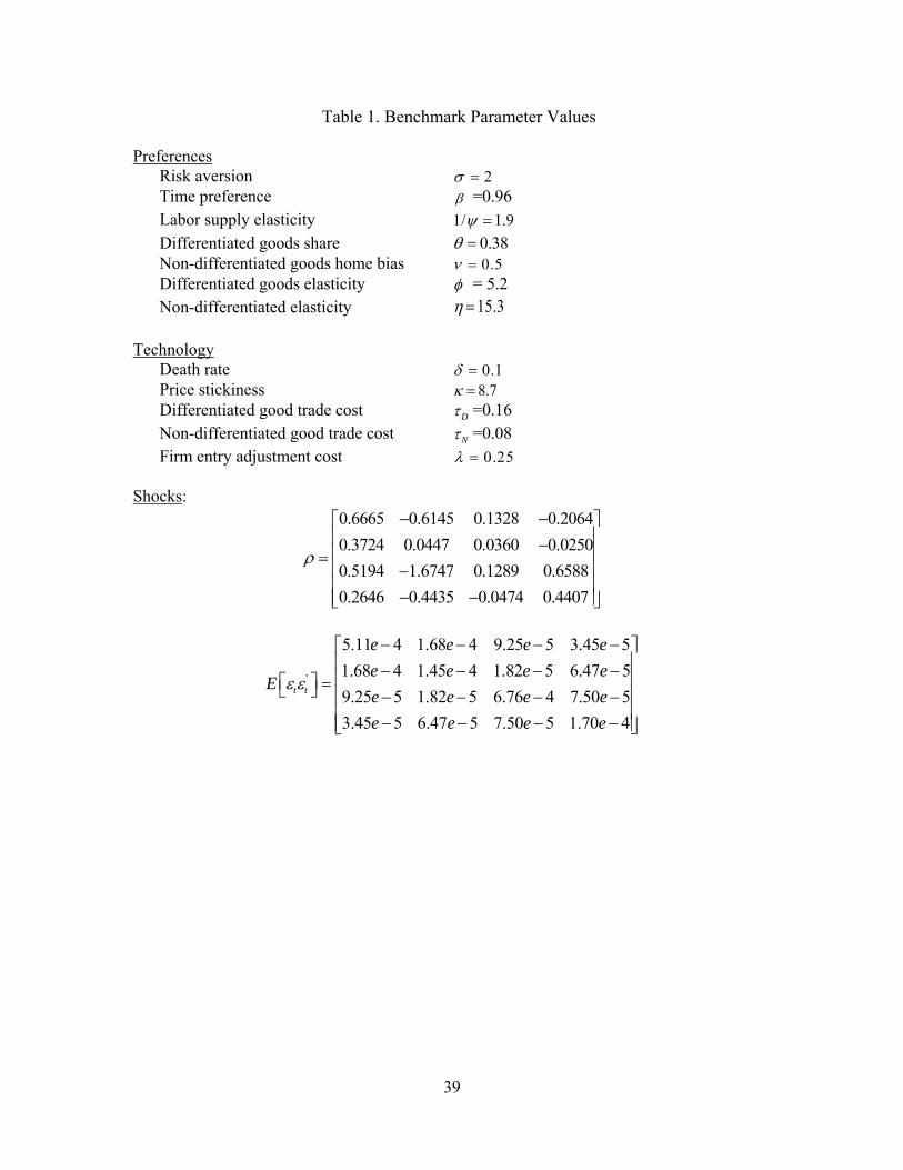
39

Table 1. Benchmark Parameter Values Preferences Risk aversion 2 Time preference =0.96 Labor supply elasticity 1/ 1.9 Differentiated goods share 0.38 Non-differentiated goods home bias 0.5 Differentiated goods elasticity = 5.2 Non-differentiated elasticity 15.3 Technology Death rate 0.1 Price stickiness 8.7 Differentiated good trade cost D =0.16 Non-differentiated good trade cost N =0.08 Firm entry adjustment cost 0.25 Shocks:

0.6665 0.6145 0.1328 0.2064

0.3724 0.0447 0.0360 0.0250

0.5194 1.6747 0.1289 0.6588

0.2646 0.4435 0.0474 0.4407

'

5.11 4 1.68 4 9.25 5 3.45 5

1.68 4 1.45 4 1.82 5 6.47 5

9.25 5 1.82 5 6.76 4 7.50 5

3.45 5 6.47 5 7.50 5 1.70 4

t t

e e e e

e e e eE

e e e e

e e e e

40

Table 2a: Unconditional Means under Alternative Policies symmetric

stabilization foreign fixed exchange rate

% difference

n 1.967 1.980 0.63 n* 1.951 1.936 -0.73

H 0.573 0.576 0.61

F 0.569 0.566 -0.56 ym 0.469 0.472 0.68 yd 0.606 0.604 -0.34 ym* 0.466 0.464 -0.58 yd* 0.608 0.612 0.53 c 0.982 0.982 0.00 c* 0.981 0.981 -0.03 p(h) 1.186 1.193 0.60 p*(f) 1.267 1.192 -5.91 w 0.959 0.964 0.60 w* 1.024 0.963 -5.91 p(h)/w 1.239 1.239 0.00 p*(f)/w* 1.238 1.239 0.07 p(h)/pdh 1.239 1.239 0.00 p*(f)/pdf* 1.238 1.239 0.07 rer 1.000 1.000 0.01 TOT-Man 1.001 1.001 0.01 TOT-total 1.000 1.002 0.38 Results come from a stochastic simulation of a second-order approximation to the model.

H represents the share of differentiated goods in overall exports of the home country, and it is computed

* * * *

,1

* * * * * * *, , ,1

( )

( )

t t Kt AC tt

Htt Kt AC t Ht Ht AC H tt t

p h n c h d h d h

p h n c h d h d h P C D

;

Ft represents the counterpart for the foreign country.

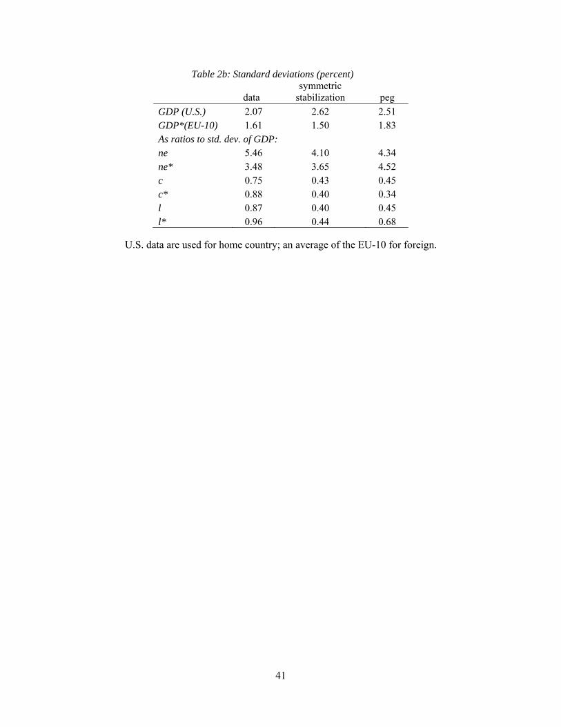
41

Table 2b: Standard deviations (percent)

data symmetric

stabilization peg

GDP (U.S.) 2.07 2.62 2.51 GDP*(EU-10) 1.61 1.50 1.83 As ratios to std. dev. of GDP: ne 5.46 4.10 4.34 ne* 3.48 3.65 4.52 c 0.75 0.43 0.45 c* 0.88 0.40 0.34 l 0.87 0.40 0.45 l* 0.96 0.44 0.68

U.S. data are used for home country; an average of the EU-10 for foreign.

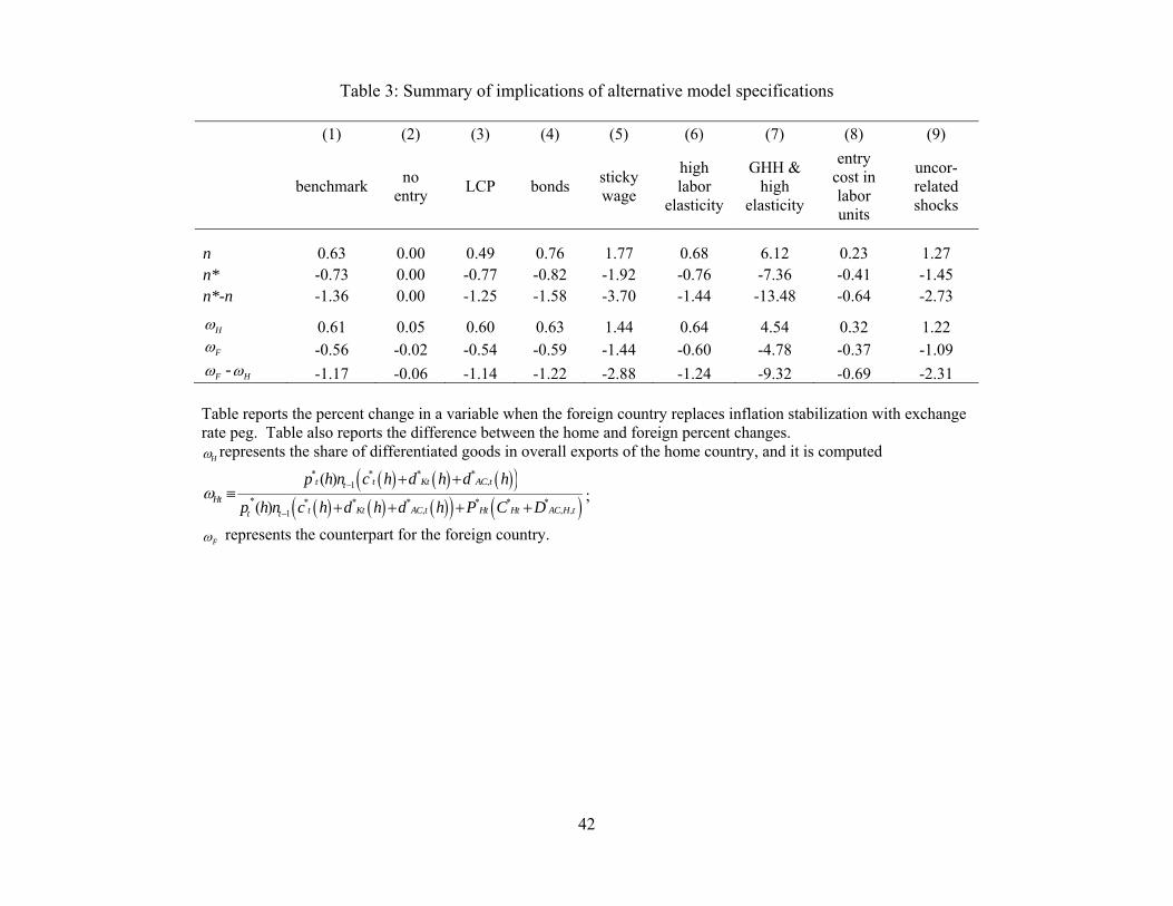
42

Table 3: Summary of implications of alternative model specifications

(1) (2) (3) (4) (5) (6) (7) (8) (9)

benchmarkno

entry LCP bonds

sticky wage

high labor

elasticity

GHH & high

elasticity

entry cost in labor units

uncor-related shocks

n 0.63 0.00 0.49 0.76 1.77 0.68 6.12 0.23 1.27 n* -0.73 0.00 -0.77 -0.82 -1.92 -0.76 -7.36 -0.41 -1.45 n*-n -1.36 0.00 -1.25 -1.58 -3.70 -1.44 -13.48 -0.64 -2.73

H 0.61 0.05 0.60 0.63 1.44 0.64 4.54 0.32 1.22

F -0.56 -0.02 -0.54 -0.59 -1.44 -0.60 -4.78 -0.37 -1.09

F - H -1.17 -0.06 -1.14 -1.22 -2.88 -1.24 -9.32 -0.69 -2.31

Table reports the percent change in a variable when the foreign country replaces inflation stabilization with exchange rate peg. Table also reports the difference between the home and foreign percent changes.

H represents the share of differentiated goods in overall exports of the home country, and it is computed

* * * *

,1

* * * * * * *, , ,1

( )

( )

t t Kt AC tt

Htt Kt AC t Ht Ht AC H tt t

p h n c h d h d h

p h n c h d h d h P C D

;

F represents the counterpart for the foreign country.

43

Table 4: Summary of implications of alternative shocks

(1) (2) (3) (4)

Money demand shocks

taste shocks

tax shocks

all four shocks

n 0.00 -0.01 0.45 1.06 n* 0.00 0.00 -0.80 -1.53 n*-n 0.00 0.02 -1.25 -2.59

H 0.00 0.00 0.56 1.17 F 0.00 0.00 -0.32 -0.88

H -F 0.00 0.00 -0.88 -2.05

Table reports the percent change in a variable when the foreign country replaces inflation stabilization with exchange rate peg. Table also reports the difference between the home and foreign percent changes.

H represents the share of differentiated goods in overall exports of the home country, and it is computed

* * * *

,1

* * * * * * *, , ,1

( )

( )

t t Kt AC tt

Htt Kt AC t Ht Ht AC H tt t

p h n c h d h d h

p h n c h d h d h P C D

;

F represents the counterpart for the foreign country.

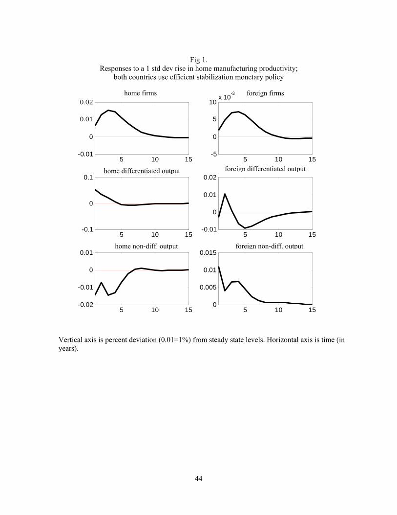
44

Fig 1.

Responses to a 1 std dev rise in home manufacturing productivity; both countries use efficient stabilization monetary policy

Vertical axis is percent deviation (0.01=1%) from steady state levels. Horizontal axis is time (in years).

5 10 15-0.01

0

0.01

0.02lln

5 10 15-5

0

5

10x 10

-3 lnstar

5 10 15-0.1

0

0.1lym

5 10 15-0.01

0

0.01

0.02lymstar

5 10 15-0.02

-0.01

0

0.01lyd

5 10 150

0.005

0.01

0.015lydstar

home firms

home non-diff. output

home differentiated output

foreign firms

foreign differentiated output

foreign non-diff. output

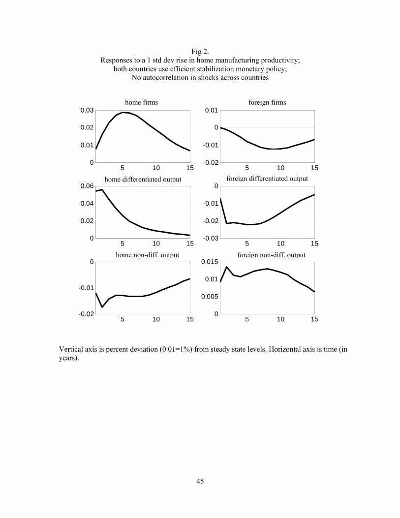
45

Fig 2. Responses to a 1 std dev rise in home manufacturing productivity;

both countries use efficient stabilization monetary policy; No autocorrelation in shocks across countries

Vertical axis is percent deviation (0.01=1%) from steady state levels. Horizontal axis is time (in years).

5 10 150

0.01

0.02

0.03lln

5 10 15-0.02

-0.01

0

0.01lnstar

5 10 150

0.02

0.04

0.06lym

5 10 15-0.03

-0.02

-0.01

0lymstar

5 10 15-0.02

-0.01

0lyd

5 10 150

0.005

0.01

0.015lydstar

home firms

home non-diff. output

home differentiated output

foreign firms

foreign differentiated output

foreign non-diff. output

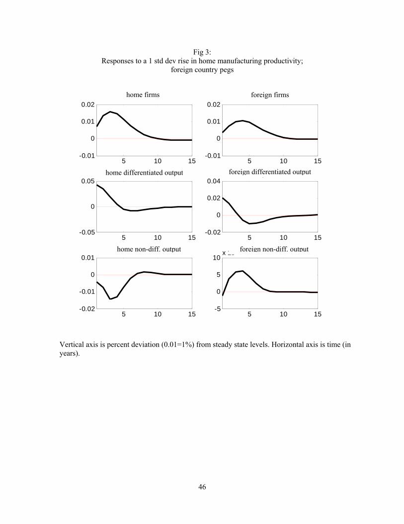
46

Fig 3: Responses to a 1 std dev rise in home manufacturing productivity;

foreign country pegs

Vertical axis is percent deviation (0.01=1%) from steady state levels. Horizontal axis is time (in years).

5 10 15-0.01

0

0.01

0.02lln

5 10 15-0.01

0

0.01

0.02lnstar

5 10 15-0.05

0

0.05lym

5 10 15-0.02

0

0.02

0.04lymstar

5 10 15-0.02

-0.01

0

0.01lyd

5 10 15-5

0

5

10x 10

-3 lydstar

home firms

home non-diff. output

home differentiated output

foreign firms

foreign differentiated output

foreign non-diff. output

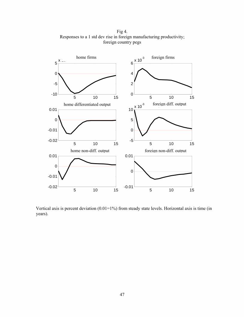
47

Fig 4. Responses to a 1 std dev rise in foreign manufacturing productivity;

foreign country pegs

Vertical axis is percent deviation (0.01=1%) from steady state levels. Horizontal axis is time (in years).

5 10 15-10

-5

0

5x 10

-3 lln

5 10 150

2

4

6x 10

-3 lnstar

5 10 15-0.02

-0.01

0

0.01lym

5 10 15-5

0

5

10x 10

-3 lymstar

5 10 15-0.02

-0.01

0

0.01lyd

5 10 15-0.01

0

0.01lydstar

home firms

home non-diff. output

home differentiated output

foreign firms

foreign diff. output

foreign non-diff. output