Embed Size (px)
Citation preview

Beyond Control
Acoustics of sound recording control rooms – past, present and future

Beyond Control
Acoustics of sound recording control rooms – past, present and future
FAGO report nr: 03.23.G
B.J.P.M. van Munster 447662April 1 2003
Eindhoven University of Technology, the NetherlandsDepartment of ArchitecturePhysical aspects of the built environment group (FAGO)
Graduation committee
Dr. Ir. H.J. Martin (chairman)Prof. Dr. A. Kohlrausch
Ir. C.C.J.M. HakIr. W.C.J.M. Prinssen

ABSTRACT
3
Summary
Since the beginning of stereophonic sound reproduction in the nineteen fifties, the concerns about the importanceof an acoustically well designed control room has increased. Typically for the quality of a well designed controlroom is the fact that the listener has to be able to listen critically to a certain recording. Therefore the interactionbetween psychoacoustical, roomacoustical and electroacoustical issues is very important. In this document thedifferent approaches are extensively considered, whereby the roomacoustical aspects are emphasised.
To obtain a good insight about what really is important in order to be able to listen critically this thesis startswith a consideration of the human hearing system. Besides explaining how the ear works, also our perception ofthe acoustical environment is described whereby the control room related issues are emphasised.Subsequently the room acoustics is discussed. Much attention will be paid to the problems regarding thegeometry of a control room. Here the low frequency sound energy plays a key role. Furthermore an elementarydescription is presented of possible material applications in a control room.Finally the electroacoustical design of the control room is considered. Therefore attention has been paid to theplacement of the loudspeakers relative to the critical listening position.
Based on this theoretical background several design philosophies evolved over the years. The most importantphilosophies which have been published since 1960 are extensively described and analysed.
Finally measurements in several Dutch control rooms were performed which have been designed by well knownDutch designers. The control rooms under test were measured extensively with microphone positions placed on agrid consisting of 15 measurement positions. Based on these measurements several important room acousticalparameters were computed such as the interaural cross correlation IACC, and the reverberation time T30.
The IACC calculations revealed that there are three important stages as a result of the interaural time andintensity differences. In the lower frequencies the IACC is approximately 0.95 and in the higher frequencies theIACC is approximately 0.50. In between a transition zone can be observed. Furthermore the calculationsrevealed that the contribution of late energy, i.e. after 80 ms, to the IACC is insignificant.
The results of the reverberation time measurements revealed that in the lower frequencies all control roomsunder test met the generally used recommendations by the ITU and EBU. In the higher frequencies the controlrooms did not all meet these criteria. It seems that this is volume dependent.
Moreover the measurements have been compared to the Bonello criterion. In order to make an attempt to qualifythe acoustical quality of a control room objectively, the rms-values of the frequency response are calculated in1/3-octave bands. According to two methods single number indications (SNI) have been computed to qualify thecontrol room. Although the methods are quite rough calculations, the results agree well with the criteria asproposed by Bonello.
In Dutch:
Sinds de opkomst van de stereofonische geluidreproductie in het begin van de jaren vijftig is de realisering vanhet belang van akoestisch goed ontworpen controle ruimte toegenomen. Kenmerkend voor de kwaliteit van eengoede controle ruimte is dat de luisteraar in staat moet zijn om uiterst kritisch naar een opname te kunnenluisteren. Daartoe is het samenspel tussen psycho akoestische, ruimte akoestische en elektro akoestischefactoren van groot belang. In dit verslag worden deze verschillende invalshoeken uitvoerig beschouwd waarbijde nadruk ligt bij de ruimte akoestische aandachtspunten.
Om een goed inzicht te krijgen in wat nu precies belangrijke aandachtsgebieden zijn voor het kritisch kunnenluisteren wordt allereerst een beschouwing van het menselijk oor gegeven. Naast het beschrijven hoe wij horen,wordt beschreven hoe wij geluid waarnemen en wat hierin belangrijk is voor een controle ruimte.Vervolgens wordt ten aanzien van de ruimte akoestiek van een controle ruimte uitvoerig de problematiek omtrentde geometrie van de ruimte behandeld. Met name het laagfrequente geluid speelt hierin een sleutelrol.Daarnaast wordt een basale beschrijving gegeven van mogelijke materiaaltoepassingen voor een controleruimte.Tot slot wordt ook het elektro akoestisch ontwerp van de controle ruimte beschouwd. Met name de plaatsing vande luidsprekers ten opzichte van de kritische luisterpositie speelt hierin een belangrijke rol.
ABSTRACT
4
Gebaseerd op deze theoretische achtergronden zijn in de loop der jaren verschillende ontwerpfilosofieënontwikkeld. De belangrijkste filosofieën welke sinds 1960 zijn gepubliceerd worden uitvoerig beschreven.
Tot slot zijn er metingen uitgevoerd in diverse Nederlandse controle ruimten welke door vooraanstaandeNederlandse ontwerpers zijn ontworpen. De controle ruimten zijn uitvoerig gemeten volgens een grid bestaandeuit 15 meetposities. Aan de hand van deze metingen zijn diverse belangrijke akoestische parametersgeanalyseerd zoals de interaurale kruis correlatie, IACC en de nagalmtijd, T30,.
Uit de IACC berekeningen bleek dat er drie fasen onderscheidden kunnen worden als gevolg van de interauraletijd en intensiteits verschillen. Laag frequent is de IACC ongeveer 0,95 en hoog frequent ongeveer 0,50.Hiertussen is valt nog een transitie zone te onderscheiden. Daarnaast is uit de berekeningen gebleken dat debijdrage van de late energie, dat wil zeggen de energie na 80 ms, ten aanzien van de bepaling van de IACConbelangrijk is.
Uit de resultaten van de nagalm metingen bleek dat laag frequent alle gemeten controle ruimten voldoen aan dedoor ITU en EBU gestelde streefwaarden ten aanzien van de nagalmtijden. Hoog frequent voldoen niet allecontrole ruimten aan de gestelde streefwaarden. Dit lijkt vooral van het volume van de ruimte afhankelijk te zijn.
Bovendien zijn de metingen aan het Bonello criterium getoetst. Om een aanzet te geven tot het objectief vaststellen van de akoestische kwaliteit van een controle ruimte zijn de rms-waarden van de frequentieresponsie in1/3-octaaf banden berekend. Volgens twee methoden zijn eengetalsaanduidingen (SNI) berekend om de ruimtente kwalificeren. De resultaten van de berekeningen komen goed overeen met de criteria zoals gesteld doorBonello.

ACKNOWLEDGEMENT
5
Acknowledgement
I would like to acknowledge certain people who have been very important to me in the last year in order tocomplete this project. First of all I am very grateful to Ben Kok and Alex Balster for their support during theproject and for sharing valuable experiences and insights with me. Also I want to acknowledge them togetherwith the owners of the control rooms for the opportunity they gave me to measure extensively in the controlrooms.In contrast to most graduating students at the acoustics laboratory, I did not work at the laboratory but at theoffice of Prinssen en Bus Raadgevende Ingenieurs B.V., acoustic consultants in Uden, the Netherlands.Therefore special thanks to them for the possibility they gave me to work at their office. Moreover I want toacknowledge all the colleagues at the office for their support in any way during the last year.Last but not least special thanks to the graduation committee for their valuable discussions, critics and inputduring the project.
This is also the right moment to thank my parents for their support and faith in me, not only during thegraduation project but also next to my study.
Bjorn van Munster
TABLE OF CONTENS
6
Table of contents
SUMMARY............................................................................................................................................................ 3
ACKNOWLEDGEMENT .................................................................................................................................... 5
TABLE OF CONTENTS ...................................................................................................................................... 6
0. INTRODUCTION ......................................................................................................................................... 9
0.1. STRUCTURE OF THE THESIS....................................................................................................................... 9
1. HUMAN HEARING SYSTEM .................................................................................................................. 11
1.1. INTRODUCTION....................................................................................................................................... 111.2. THE ANATOMY OF THE HUMAN EAR........................................................................................................ 11
1.2.1. Outer ear ....................................................................................................................................... 121.2.2. Middle ear ..................................................................................................................................... 121.2.3. Inner ear ........................................................................................................................................ 13
1.3. PERCEPTION OF SOUND........................................................................................................................... 141.3.1. Sound localisation ......................................................................................................................... 14
1.3.1.1. Duplex theory ........................................................................................................................................141.3.1.2. Pinna reflections ....................................................................................................................................151.3.1.3. Head movements ...................................................................................................................................16
1.3.2. Coloration...................................................................................................................................... 161.3.2.1. Comb filtering .......................................................................................................................................16
1.3.3. Stereophonic perception ................................................................................................................ 171.3.3.1. Haas- or precedence effect.....................................................................................................................17
1.3.4. Image shift of phantom sources ..................................................................................................... 191.3.5. Interaural cross correlation (IACC).............................................................................................. 20
2. ARCHITECTURAL DESIGN ISSUES OF A CONTROL ROOM ....................................................... 22
2.1. INTRODUCTION....................................................................................................................................... 222.2. RECOMMENDATIONS .............................................................................................................................. 222.3. GEOMETRY OF THE ROOM....................................................................................................................... 23
2.3.1. Eigenmodes.................................................................................................................................... 232.3.2. Distribution of the eigenmodes...................................................................................................... 232.3.3. Optimisation of the mode distribution ........................................................................................... 26
2.3.3.1. Room dimensions ..................................................................................................................................262.3.3.2. Bonello criterion....................................................................................................................................302.3.3.3. Distributed mode optimization ..............................................................................................................31
2.4. FINISHING OF THE ROOM ........................................................................................................................ 332.4.1. Diffusion / Diffraction.................................................................................................................... 33
2.4.1.1. Conventional diffusion ..........................................................................................................................332.4.1.2. Schroeder diffusors................................................................................................................................34
2.4.2. Absorption ..................................................................................................................................... 352.4.2.1. Porous absorbers....................................................................................................................................352.4.2.2. Resonators .............................................................................................................................................37
2.5. LOUDSPEAKER ARRANGEMENT .............................................................................................................. 422.5.1. Introduction ................................................................................................................................... 422.5.2. Arrangement types......................................................................................................................... 42
2.5.2.1. Stereo loudspeaker arrangement ............................................................................................................422.5.2.2. Multi channel loudspeaker arrangement ................................................................................................452.5.2.3. Low frequency loudspeaker placement..................................................................................................462.5.2.4. Height of the loudspeakers ....................................................................................................................46
2.5.3. Near field or wall mounted loudspeakers ...................................................................................... 47
3. DESIGN PHILOSOPHIES......................................................................................................................... 48
3.1. INTRODUCTION....................................................................................................................................... 483.2. HORN COUPLED SOFFITS – PUTNAM (1960) ........................................................................................... 483.3. INERT ROOM APPROACH – VEALE (1973) ............................................................................................... 50

TABLE OF CONTENS
7
3.3.1. Design criterion............................................................................................................................. 503.3.1.1. Auditory system.....................................................................................................................................503.3.1.2. Materials................................................................................................................................................51
3.3.2. Design procedure .......................................................................................................................... 513.4. HORN COUPLED ROOM – RETTINGER (1977) .......................................................................................... 52
3.4.1. Shape of the room.......................................................................................................................... 523.4.2. Reverberation time ........................................................................................................................ 53
3.5. LIVE-END-DEAD-END (LEDE) APPROACH – DAVIS (1981) ................................................................... 543.5.1. Background of the approach ......................................................................................................... 54
3.5.1.1. TEF measurements ................................................................................................................................543.5.1.2. Initial time delay gap .............................................................................................................................553.5.1.3. Haas zone ..............................................................................................................................................563.5.1.4. Frequency analyses................................................................................................................................56
3.5.2. LEDE control room criteria .......................................................................................................... 573.6. REFLECTION FREE ZONE (RFZ) APPROACH – D’ANTONIO (1984).......................................................... 57
3.6.1. RFZ design method........................................................................................................................ 583.6.1.1. RFZ in a surround sound studio.............................................................................................................60
3.7. PSYCHOACOUSTIC APPROACH – WRIGHTSON (1984) ............................................................................. 603.7.1. Background of the approach ......................................................................................................... 60
3.7.1.1. Psychoacoustic considerations...............................................................................................................603.7.1.2. Application to control room design .......................................................................................................61
3.7.2. Design criteria ............................................................................................................................... 623.8. CONTROLLED IMAGE DESIGN (CID) – WALKER (1993)......................................................................... 62
3.8.1. Design methodology ...................................................................................................................... 623.8.1.1. Extension for multi-channel control rooms............................................................................................64
3.9. SURROUND SOUND APPROACH – WSDG (1999).................................................................................... 653.9.1. Design goals for a surround sound control room.......................................................................... 65
4. ROOM ACOUSTICAL MEASUREMENTS............................................................................................ 66
4.1. INTRODUCTION....................................................................................................................................... 664.2. DESIGN APPROACHES OF THE CONTROL ROOMS UNDER TEST.................................................................. 66
4.2.1. Suppression of the reflections – Alex Balster ................................................................................ 664.2.1.1. Loudspeakers.........................................................................................................................................664.2.1.2. Symmetrical room .................................................................................................................................664.2.1.3. Suppression of reflections......................................................................................................................674.2.1.4. Reverberation time ................................................................................................................................67
4.2.2. Reflection control – Ben Kok......................................................................................................... 674.2.2.1. Suppression of the early reflections.......................................................................................................674.2.2.2. Loudspeaker independent design...........................................................................................................674.2.2.3. Even spectral and spatial distribution of the resonance frequencies ......................................................684.2.2.4. Large sweet spot ....................................................................................................................................68
4.3. CONTROL ROOMS UNDER TEST ............................................................................................................... 684.4. DESCRIPTION OF THE MEASUREMENTS ................................................................................................... 68
4.4.1. Measurement positions .................................................................................................................. 694.4.2. Procedure ...................................................................................................................................... 69
4.4.2.1. Artificial head........................................................................................................................................704.5. BINAURAL MEASUREMENTS ................................................................................................................... 70
4.5.1. Inter Aural Cross Correlation ....................................................................................................... 704.5.1.1. Goal .......................................................................................................................................................704.5.1.2. Results ...................................................................................................................................................714.5.1.3. Discussion .............................................................................................................................................72
4.5.2. Comparison of the different positions within a room .................................................................... 734.5.2.1. Goal .......................................................................................................................................................734.5.2.2. Results ...................................................................................................................................................734.5.2.3. Discussion .............................................................................................................................................74
4.5.3. Influence of the measurement length on the results of the IACC calculation ................................ 754.5.3.1. Goal .......................................................................................................................................................754.5.3.2. Method ..................................................................................................................................................764.5.3.3. Results and discussion ...........................................................................................................................76
4.6. REVERBERATION TIMES.......................................................................................................................... 774.6.1. Introduction ................................................................................................................................... 774.6.2. Comparison of the measurement results to the recommendations................................................. 77
4.6.2.1. Goal .......................................................................................................................................................77

TABLE OF CONTENS
8
4.6.2.2. Results ...................................................................................................................................................784.6.2.3. Discussion .............................................................................................................................................79
4.6.3. Comparison of microphones for calculation of the reverberation time......................................... 804.6.3.1. Goal .......................................................................................................................................................804.6.3.2. Results ...................................................................................................................................................804.6.3.3. Discussion .............................................................................................................................................80
4.6.4. In situ verification of the Bonello criterion.................................................................................... 814.6.4.1. Goal .......................................................................................................................................................814.6.4.2. Procedure...............................................................................................................................................814.6.4.3. Qualification methods............................................................................................................................824.6.4.4. Results ...................................................................................................................................................824.6.4.5. Discussion .............................................................................................................................................83
5. CONCLUSIONS AND RECOMMENDATIONS..................................................................................... 85
5.1. OVERALL CONCLUSION .......................................................................................................................... 855.2. CONCLUSIONS ........................................................................................................................................ 85
5.2.1. Chapter 1: Human hearing system ................................................................................................ 855.2.2. Chapter 2: Architectural design issues of a control room............................................................. 865.2.3. Chapter 3: Design philosophies ................................................................................................... 865.2.4. Chapter 4: Room acoustical measurements .................................................................................. 86
5.2.4.1. Procedure...............................................................................................................................................865.2.4.2. Binaural measurements..........................................................................................................................875.2.4.3. Reverberation measurements.................................................................................................................875.2.4.4. Verification of the Bonello criterion......................................................................................................87
5.3. RECOMMENDATIONS .............................................................................................................................. 885.3.1. Chapter 2: Architectural design issues of a control room............................................................. 885.3.2. Chapter 4: Room acoustical measurements .................................................................................. 88
5.3.2.1. Procedure...............................................................................................................................................885.3.2.1. Binaural measurements..........................................................................................................................885.3.2.2. Reverberation measurements.................................................................................................................885.3.2.3. Verification of the Bonello criterion......................................................................................................88
EPILOGUE.......................................................................................................................................................... 90
BIBLIOGRAPHY................................................................................................................................................ 91
Introduction Chapter 0
9
0. Introduction
Two years ago, September 2000, I started a project at the acoustics laboratory of the Eindhoven University ofTechnology. The aim of the project was to design a studio which could be used as a laboratory for multisensoryresearch at the center for user-system interaction.
During the project I noticed the relevance of some acoustical issues, but more important, I noticed that there wasnot really a fundamentally scientific approach to the design of a studio or control room. In the past there has beenresearch to aspects which are also applied in the designs of studios, e.g. room dimensions, localisation etc., butthis has never been done in the context of an integral approach to a critical listening environment.
Besides missing the theoretical scientific principles of the design of control rooms and studios it also appeared tome that not too many measurements had been performed in these acoustical environments. Many rooms are builtwith a certain philosophy of the designer, in some cases combined with some ideas of the user, and if both aresatisfied with the result, the project is finished and will be qualified as successful. This lack of a scientificallybased approach resulted in the starting point of the graduation project.
Primarily the aim of the project was to survey the design concepts of control rooms. Here the main interest wasto find out what issues are really important in the design and how the design concepts of the control rooms haveevolved over the years.Besides an extensive literature study also acoustical measurements have been performed in order to make a startwith defining the quality of a control room objectively by measurements. Indeed, the control rooms weresubjectively all qualified as good, while they differ in their concepts.
In the preceding both terms, control room and studio, are used. Essentially these type of rooms are not the same.To distinguish both rooms, in this report the definitions presented by d’Antonio [1] are used. The essence of thedistinction between control rooms and studios is the usage of the room. A studio is referred to as a productionroom in which, e.g., the music is played. In these rooms the acoustics contribute to the character of the sound.On the other hand the control rooms are referred to as the reproduction rooms. Here the acoustics provide aneutral environment to listen to pre-recorded information. This project focussed on the reproduction or controlrooms.
0.1. Structure of the thesis
In the first chapter general issues regarding the human hearing system are discussed. Although it seems morerelated to biological or psychoacoustics rather than architectural acoustics, it is very important to understandthese phenomena to a great extent. In many cases issues which are discussed in this chapter are fundaments, thebases for design decisions, although we are not always aware of it. When we know the reason why somedecisions are made, we are able to protect ourselves against mistakes in the design and can save the customer’smoney. Moreover, by knowing the adjacent ideas we are able to optimise some commonly used solutions.
In the subsequent chapter the architectural considerations regarding the design of control rooms are discussed.There are no standards in which aspects of a control room design are placed on a record. However some largeEuropean broadcasting corporations like the EBU and ITU have made recommendations regarding the design ofa control room. The chapter starts with an overview of the existing recommendations and their main.
Due to very stringent perceptual requirements, especially in critical environments like control rooms, there aretypical acoustical solutions. Therefore in the subsequent part of the chapter the most important physics andarchitectural principles are discussed such as room geometry, absorption and reflection. The design of a controlroom is a process of optimisation between loudspeakers, room and listener. To optimise the design of a controlroom, it is also important to be aware of the loudspeakers and their interaction with the room. Although thistends to be more a topic of electroacoustics, some important considerations regarding the loudspeakers in thecontrol room are also presented in this chapter.
Chapter three starts with a brief historical overview of the development of the control room. During the years theway of reproducing sound has evolved from monophonic control rooms to control rooms suited for stereoreproduction and in the last decennium surround sound has become more popular.

Introduction Chapter 0
10
In the past, several authors have presented general approaches for the design of a control room. These conceptsare still applied by designers all over the world. Although these concepts are not the golden solutions for acontrol room design, they all have proven there quality, despite the enormous contradictions between them. Inthe subsequent part of chapter three the most important philosophies are discussed in greater detail.
The latter part of the graduation project, acoustical measurements were performed in six control rooms. Three ofthem were designed by Ben Kok, three of them by Alex Balster. Both are well-known Dutch designers with analmost contradictory philosophy. The designs of the former rooms are based on controlling the reflections, thelatter one’s are based on suppression of the reflections. This results in a completely different layout of the plan ofa control room. A profound description of their philosophy is given in chapter four of this thesis.Furthermore in this chapter the measurement results are discussed. The measurements have been performed byplacing the microphones at 15 different positions according to a 5x3 matrix in every control room. This resultedin an overflow of data which could be extracted from the impulse responses. Only the most relevant parametersregarding this thesis are discussed such as the interaural cross correlation IACC and the reverberation time T30.Besides evaluating the regular parameters, also the so called Bonello criterion is applied to the in situmeasurements in order to find out to what extent this can be a starting point for qualifying the acoustical qualityof a control room objectively.

Human hearing system Chapter 1
11
1. Human hearing system
1.1. Introduction
Although it seems to be a more biological than physical matter, the perception of sound needs to be understoodto a great extent in order to form and understand the theory of important issues and decisions to be made duringthe design process of a control room. A lot has been written about the way the ear works, how we perceivesound and what psychoacoustical issues are important in our perception of a certain sensation. This chapter willgive a brief summary of the most important issues. In the first paragraph the anatomy of the human ear ispresented. Thereafter the perception of the ear will be discussed.
1.2. The anatomy of the human ear
The human ear can be divided in three different parts, each with their own characteristics and functions. First thesound will be received by the outer ear. Hereafter the sound is directed to the middle ear. After impedanceadjustments are made by the ossicles, the sound is directed to the inner ear where it is transduced into neuralsignals. The figure below presents the anatomy of the human ear.
Figure 1 : Overview of the outer, middle and inner ear. [From: Durrant and Lovrinic, 1995]

Human hearing system Chapter 1
12
1.2.1. Outer ear
The outer ear consists of the pinna, the ear canal and the eardrum (tympanic membrane). The primary function ofthe pinna is the reception of sound. As the sound is received by the pinna it is collected frequency dependent anddirected to the ear canal. This also results in a amplification of the received sound [3].For a long time it was assumed that the only function of the pinna was to collect sound and direct it to the earcanal. Research showed that the pinna is also very important for the localisation of a sound source [1]. Especiallyour perception of the elevation of a sound source is determined by the spectral filtering of the pinna. This is moreelaborated in paragraph 1.3.1.2.
After receiving the sound by the pinna it is directed to the ear canal. The ear canal as a resonance system alsoamplifies the sound. Here the amplification is very effective since the air pressure can build up at the tympanicmembrane. The strongest amplification occurs for a frequency for which the wavelength is equal to one fourth ofthe ear-canal length, typically 3.5 kHz. Besides the ear canal also has a protectoral function, e.g. per epitheliumcovered with cilia [3]. After passing through the ear canal, the sound arrives at the eardrum. Here the sound istransmitted to the middle ear.
1.2.2. Middle ear
The middle ear consists of the ossicles: malleus, incus and the stapes, which is the smallest bone in our body.The middle ear is connected to the inner ear by the oval window and the round window. For the relaxation ofhigh pressure in the ear the middle ear is also connected to the nose by the Eustachian tube.
Figure 2: Middle- and inner ear [From: Warren, 1999]
Like the outer ear, the middle ear also has a protectoral function. The middle ear has to protect against too highsound pressure levels. Therefore the ossicles are fixed to the rest of the skull by small muscles. Dependent on thesound pressure level these muscles will contract more or less and fix when the pressures get too high [3].
Another characteristic of the middle ear is that the sound is amplified by an impedance adjustment. This can beexplained as follows. The cochlea is filled with a liquid with a much larger impedance relative to the air in theear canal. When the cochlea was connected directly to the eardrum, there would be a large impedance difference.This typically leads to reflection of the incoming sound at the eardrum. By adjusting the impedance differencebetween the two media the amount of reflected energy can be reduced, so the amount of energy transmitted tothe cochlea will be increased.

Human hearing system Chapter 1
13
The mechanism which adjusts the impedance difference between the ear canal and the cochlea is presented inFigure 3. As can be seen in the figure, on the one hand the impedance adjustment is due to the proportionbetween the area of the eardrum and the oval window, i.e. this proportion is 18.6 : 1. On the other hand theproportion of the distance from the eardrum to the centre of gravity of the malleus and from this centre of gravityto the oval window plays is important. This has a proportion of 1.3 : 1. Both the mechanisms result in a factor 24of amplitude gain or 576 in intensity which agrees with a 28 dB amplification [3].
Figure 3 : Schematic overview of the impedance adjustment mechanism in the middle ear. [From:Durrant and Lovrinic, 1995]
1.2.3. Inner ear
The inner ear, also presented in Figure 2, consists of the cochlea where the basilar membrane comprises haircells which are connected to the auditory nerve.When a certain sound pressure strikes the eardrum, it is transduced into vibrations, The middle ear ossiclestransmit these vibrations to the cochlea. At the oval window, the stapes drives the fluid in the cochlea andproduces a travelling wave along the basilar membrane. On the cochlea sensory receptors are located whichtransform the fluid vibration into a neural code.The basilar membrane is very flexible and operates as a spectral filter. Every location on the membrane canmove more or less independently and has its maximum sensitivity for a certain frequency. The further away fromthe oval window, the lower the frequency the basilar membrane is sensitive to.
Figure 4 : Envelope of the travelling wave on the basilar membrane. The further away from the stapes,the lower the filtering frequency. [From: Békésy, 1960]

Human hearing system Chapter 1
14
1.3. Perception of sound
The field of small room acoustics, especially the design of critical listening environments, is very closely relatedto the psychoacoustic research field. Many of the decisions made to achieve the proper acoustic solution for acertain problem are directly derived from our perceptual experiences. This paragraph will therefore discuss theperceptual issues which are important in the acoustical design of a critical listening environment.
1.3.1. Sound localisation
When we are listening to a concert and e.g. the violins are seated halfway left the stage, it is important that wealso perceive the violins acoustically coming from that direction. This process of correctly perceiving theauditory event is called sound localisation. Especially while reproducing a recording in a control room it isimportant that the recording can be reproduced as precise as possible, in other words the localisation has to begood. By knowing how localisation works and how it can be disturbed, expensive errors in the design processcan be avoided.
There are several important factors regarding the localisation of a sound source. Primarily the interaural timedifferences (ITD) and interaural intensity differences (IID) give us cues of the direction of the source. Thisprocess is described with the duplex theory. We also localise a sound source by binaural frequency analysis as aconsequence of our two ears and the movement of our head. Furthermore directional cues, i.e. the elevation of asource, are given by the pinna. In the next sections these factors will be explained in more detail.
1.3.1.1. Duplex theory
According to the duplex theory the localisation of a sound source is primarily determined by the time and leveldifferences between the ears due to the shape of our head and torso.At frequencies with a wavelength shorter than the diameter of the head, that is approximately at frequenciesabove 2 kHz1, the sound will be reflected by the head. In other words, the head will shadow the sound source forone ear with respect to the other. The result is that at high frequencies, thus above 2 kHz, the sound source willprimarily be localised by interaural intensity differences between the ears.
d1=r sinq
d2=rq
q
q
q
DISTANT SOURCE
Figure 5 : Due to path differences there occur inter aural time differences. [After: Warren, 1999]
Because of the shape of our head a soundwave will bent around our head. This results in path differencesbetween both ears (see Figure 5) which are perceived as interaural time differences. Interaural time differencesare the dominant localisation cue at frequencies below say 1.5 to 2 kHz, because here the neural system does alsocode the phase of the signal and the maximum path difference between right and left ears is smaller than half aperiod of the sound signal. Above 2 kHz the path difference is longer than half a period whereby the phasecoding becomes ambiguous.
1 This frequency depends on the size of the head. Moreover it has to be noted that this actually is a transition zone from say1.5 to 2 kHz.

Human hearing system Chapter 1
15
1.3.1.2. Pinna reflections
When a sound source is placed on the median plane in front of a person, the ITD, IID and phase differences as aconsequence of the path difference between the ears are equal. When the sound source is placed behind theperson on the median plane, the ITD, IID and phase differences are also equal. Nevertheless, we are able tolocalise the sound source if it is in front or behind us. Thus besides the ITD’s and IID’s there has to be other cuesfor the localisation of a sound source.
In this respect, it appeared that the shape of the pinna plays a crucial role. As been told in the previousparagraph, it was first assumed that the only function of the pinna was to collect the sound and direct it into theear canal, the pinna appeared to be quite important regarding the localisation of sound.The surface morphology of the pinna has two important characteristics: it consists of small reflecting surfacesand it is asymmetrical. Thus every change of the angle of the incoming sound will lead to a change in delays andthus in a different reflection pattern of the incoming signal [1]. The figure below clarifies this graphically.
Figure 6: Drawings of the pinna, showing the path differences of the first reflection from a sound sourcewith a different elevation. [From: Puddie Rodgers, 1981]
Because of the angle dependent reflection pattern, the pinna actually works as a spectral filter. As can be noticedfrom the figure, the higher a source will be placed, the shorter travel difference between the direct and reflectedsound will be, and so the time delay between the two signals. This results in a higher first spectral minimumwhen a sound source is placed higher.
Figure 7 presents a pinna response of a sound source with an azimuth of 180° located below ear level. On thehorizontal axis the frequency is plotted linear in kHz, on the vertical axis the intensity is plotted from –70 to 30dB. As the figure reveals, the pinna introduces comb filtering (See paragraph 1.3.2.1). But more important is thatit reveals that above the first minimum the level is approximately 10 dB attenuated. This implies that the pinnaactually works as a low pass filter for sound coming from the back of our head [5].
Figure 7: Pinna response for a sound source positioned at 180°° azimuth and below ear level. [From:Puddie Rodgers, 1981]

Human hearing system Chapter 1
16
1.3.1.3. Head movements
A third factor which helps us to localise a sound source is the movement of our head. This process is bestexplained by using the analogy of how birds can see depth. Birds have their eyes on the side of their heads.Therefore the image they see with both eyes doesn’t match. To be able to see depth, the eye constantly takesscreenshots. The difference between the screenshots gives the bird a cue about distance and position in itsenvironment.
By humans this mechanism is applied in the ear. When the head is in a certain position there are cues, i.e. theITDs and IIDs, which characterise that position. When moving the head there is a new set of cues given. Bycomparing these with the preceding cues, we are able to determine where a certain sound is coming from.
1.3.2. Coloration
When the spectral shape of a certain sound signal changes this is perceived as coloration of the sound. Thisresults in an accentuation of particular frequencies in speech or music so that certain notes or vowel soundsassume unnatural prominence [12]. The spectral shape can be influenced by reflections or interference of two ormore signals. This is called comb filtering. In acoustics there are lots of examples which can introduce colorationsuch as room modes, speaker boundary interference, misalignment of loudspeakers and pinna reflections.
1.3.2.1. Comb filtering
The result of adding two or more identical signals with a certain time delay, viewed in the frequency domain isknown as comb filtering. An idealised drawing is given in the figure below.
Figure 8: Idealised drawing of an impulse and a subsequent reflection occurring 200 µµs later. (a) Signal inthe time domain. (b) Signal in the frequency domain. [From: Puddie Rodgers, 1981]
The time difference of 200 µs (see Figure 8) corresponds to a frequency of 5000 Hz. The spectrum of thecombined signal has maxima at integer multiples of this frequency. At odd multiples of this frequency, i.e. 2500Hz, 7500 Hz, etc., the spectrum has minima.
As a result of the comb filtering, the spectral structure of the sound will change. This change is audible ascoloration of a certain signal. Moreover, the continuous change of the spectral pattern creates the illusion ofchanging the sound source elevation [4]. This is called image shift. I.e. as a result of the comb filtering the imageshift is perceived as a movement in the vertical plane.
Because of the importance of good sound localisation and necessity of good sound reproduction in the room,comb filtering should be avoided as much as possible. This can be realised by moving the first minimum to ahigh frequency. The reciprocal relationship between the frequency and time reveals that therefore the delaybetween the signals has to be optimised: the shorter the delay, the higher the comb filter frequency will get. So toremove all the minima from the audible spectrum, the time difference should be shorter than 25µs or 8.5 mm,because then the first null in the energy frequency curve will appear above the highest (human) audiblefrequency of 20,000 Hz.

Human hearing system Chapter 1
17
In actual practice it is almost impossible to achieve this short delays by architectural solutions. Therefore in thisrespect attenuation, e.g. by absorption, or redirection, e.g. by diffusion or redirecting, of the signals is required insuch a way that the comb filtering is not perceived by the listener.
1.3.3. Stereophonic perception
In the past there has been a lot of research on the perception of stereophonic loudspeaker set-ups. Among othersthis was done by de Boer, Franssen and Blauert. The research on stereophonic perception mainly happens inanechoic rooms. The loudspeakers are placed at an angle of 30° left and right from the listener, producingcoherent signals. The signal of one of the sources will not be delayed, this is called the direct signal. The othersource will be delayed and is therefore called the delayed source. (See Figure 9)
DIRECT SOUND DELAYED SOUNDPHANTOMSOURCE
med
ian
plan
e30°
Figure 9: Example of a standard stereophonic measurement set-up.
When both sources produce an identical signal with an equal level and no delay, the auditive system interpretsthis as if the signal is produced by a phantom source, placed symmetrically with respect to the median plane [7].This effect is also called the summing localisation effect. When the signal of one of the sources will be delayed,the phantom source slowly moves towards the undelayed source. When the delaytime is between 630 µs and 1ms, the phantom source will be the undelayed source [7].
If the delaytime is more than 1 ms, the direction perceived by the auditory system is primarily determined by thesound that reaches the ear first. This is called the law of the first wavefront [7]. Thus, the crossover point fromsumming localisation to the law of the first wavefront, this is the upper limit of an auditive event where thephantom source moves due to a delay between the two sources, is between 630 µs and 1 ms [7].
To define the upper limit of the situation where the law of the first wavefront is applicable is more difficult. Thisis dependent on several factors like level differences between the sources, the type of signal, the angle of theincoming sound and the delaytime. One of the people who examined the upper limit is Haas. In the nextparagraph this will be outlined in more detail.
1.3.3.1. Haas- or precedence effect
During Haas’ examination he used speech with a level of 50 dB as the signal and delayed this signal from 1 to160 ms. The subjects had to point out whether the signal with a certain delay was experienced as disturbingregarding the speech intelligibility at that specific position in the room. Moreover they had to indicate how muchthe level of the delayed signal had to be raised to make the direct sound no longer audible. His investigationshowed that above a certain delay the auditory event was separated into two separate events [7][8].
The first auditory event is coming from the direction of the direct sound. The second event comes from thedirection of the first incoming high level reflection. This reflection is called the echo of the first event. Byrendering the delay time versus the relative level difference an echo threshold can be defined. Because of theused signal this actually is a threshold for the speech intelligibility impairment. Figure 10 shows the echo-threshold.

Human hearing system Chapter 1
18
Figure 10: A comparison of various thresholds for reflections; standard stereophonic loudspeakerarrangement, base angle αα= 80°° (data of Haas 1951, Meyer and Schodder 1952, Burgtorf 1961, Seraphim1961). [From: Blauert, 1982]
The figure shows that in case the delay is less than 32 ms, the level of the echo can be 5 dB higher relative to theprimary sound without being audible. Furthermore it shows that if the delaytime is between 5 and 30 ms, theintensity level of the delayed signal has to be at least 10 dB louder than the undelayed signal to experience thedelayed source as an echo [8].The research also revealed that if the delaytime exceeds 30 ms, the speech intelligibility will be diminished. Theecho is perceived as annoying at threshold values that intersect the curve of equal loudness at a delay time ofapproximately 65 ms and increase sharply as the delay time is decreased.When the reflected energy reaches the ear within 50 ms, this will be integrated with the direct sound andcontributes to the perceived loudness of the signal [7][8][11]. In practice this will be noticed as a broadening ofthe direct, undelayed source while the delayed source is not acoustically perceived [11].
Summarising it can be said that for delays less than 50 ms the echoes will not be perceived as troublesome, evenif the level is higher than the primary sound. The optimum in this case is nearby 20 ms. This is called the Haas-effect.During the examination of Haas, at almost the same time a comparable research was performed in the US byWallach, Newman and Rosenzweig [9]. Although the experimental methods differ, the substantial conclusionsare the same as Haas made. Wallach et al called it the precedence effect. In literature both terms are used foressentially the same effect.
By using a set of signals with the proper levels and delays, the Haas-zone can be extended. This is sometimesreferred to as the Kuttruff-effect [10]. The concept of extending the Haas-zone according to the Kuttruff-effect isgiven in the figure below. Among others this concept is applied in control rooms built according to the LEDEconcept (see paragraph 3.5).
0 10 20 30 40 50 60 70 80 90 100
Time [ms]
Leve
l [dB
]
Onedelay
Twodelays
Threedelays
Fourdelays
Figure 11: Kuttruff-effect [After: Davis, 1997]

Human hearing system Chapter 1
19
1.3.4. Image shift of phantom sources
In the past de Boer among others has done research on the influence of level- and time differences between twoloudspeakers with reference to the phantom source [6]. He placed two loudspeakers 3.5 m separated from eachother, with a listener at 3.5 m distance on the median plane between the two loudspeakers. This implies anmaximum angle between the loudspeaker and the median plane of approximately 26°.The results of his investigation are presented in the figures below.
0
8
16
24
0,0 0,5 1,0 1,5 2,0 2,5 3,0 3,5 4,0
Time difference [ms]
Ang
le [o ]
0
8
16
24
0 2 4 6 8 10 12 14
Level difference [dB]
Ang
le
Figure 12: Level- and time differences with reference to the angle with median plane. [After: de Boer,1940]
The most important conclusion drawn from his research was that in a situation in which both time- and leveldifferences occur, the differences are additive or subtractive. This implies that the perceived sound image can beincreased or decreased towards the situation in which only one of the quantities is present. Thus, with bothquantities it is possible to keep the sound image at a fixed position.This result was more profoundly researched by Meyer and Schodder. They examined which combinations oflevel- and time differences did not cause a movement of the phantom source. The results are given in the figurebelow.
Figure 13: Influence of combinations of level- and time differences on the stereophonic perception. Rrepresents the right loudspeaker plane, M the median plane and L the left loudspeaker plane. [From:Franssen, 1962]
For example, when the right speaker has a delay of 2 ms with respect to the left speaker, the level of the rightloudspeaker should be 7 dB louder than the left loudspeaker to keep the sound image in the center between thetwo loudspeakers.
As stated before, in stereophonic sound reproduction the localisation of sound sources is very important to createa stable sound image. According to the previous research of de Boer, Meyer and Schodder the time- and leveldifferences between the loudspeakers are in this respect important cues.

Human hearing system Chapter 1
20
1.3.5. Interaural cross correlation (IACC)
The sound perceived at our ears can be represented objectively with two head related impulse responses hnl,r(t)[13]. These two responses hnl(t) and hnr(t) are important regarding the localisation and spatial impression.In the median plane of the ears these two responses are, theoretically, identical. Off axis these responses are notidentical although there are still relations between them. At low frequencies these are interaural time differences,ITD, and at high frequencies, above 2000 Hz, these relations are interaural intensity differences, IID. Theinterdependence between both impulse responses can be represented by the Interaural Cross-correlation Function(IACF), Φlr(τ) , between the sound signals f1(t) and f2(t) at both ears which is defined by [13]:
(1) ( ) ( ) ( )∫+
−∞→+=Φ
T
T rlTlr dttftfT
ô τ''
21
lim ms1≤τ
where fl’(t) and fr
’(t) are approximately obtained signals by fl,r(t) after passing through an A-weighted networkwhich corresponds to the ear sensitivity. T represents the time interval of interest, usually this is the reverberationtime T60 [s]. The time interval of 1 ms is chosen because this is the maximum interval delay between both ears.
The normalised IACF, φlr(τ), is defined by
(2) ( ) ( )( ) ( )00 rrll
lrlr
ô
ΦΦΦ=τφ
where Φll(0) and Φrr(0) represent the auto correlation function at τ=0 for the left and right ear. In other wordsthis is the sound energy arriving, at respectively, the left and right ear [13]. The denominator in general is thegeometrical mean of the sound energies arriving at both ears.
For discrete reflections which arrive after the direct sound the normalised IACF can be expressed by
(3) ( )( )( )( )
( )( ) ( )( )∑∑∑
==
=
ΦΦ
Φ=
N
n
nrr
N
n
nll
N
n
nlrN
lr
AA
A
02
02
02
00
ττφ
where A is the amplitude of the nth reflection relative to the amplitude of the direct sound. Φlr(n)(τ) the IACC of
the nth reflection and Φll(n)(τ) and Φrr
(n)(τ) the sound energies arriving at respectively the left and right ear.
The maximum value of the IACF represents the Interaural Cross Correlation IACC. Therefore mathematicallythe IACC is defined as [13]:
(4) ( )max
IACC τφlr=
for the maximum interaural time delay |τ| ≤ 1ms
As shown in the Figure 14, the interaural delay time of the maximum is denoted τIACC. When τIACC = 0 usually afrontal sound image and well-balanced sound field are perceived [13].The width of the IACF, WIACC, is defined by the interval of delay time during which the function stays above athreshold value δ. In fact this corresponds to the JND of the IACC. According to Ando therefore the ApparentSource Width (ASW), as defined by Beranek in [14], may be perceived as a directional range correspondingmainly to the WIACC. For a sound field with τIACC = 0, the width of the interaural cross-correlation function isapproximated by
(5)
−
∆≈ −
IACCW
cIACC
δω
1cos4 1

Human hearing system Chapter 1
21
-1,0
0,0
1,0
-1,0 -0,5 0,0 0,5 1,0
ττ [ms]
φφ
lr( ττ)
φφ lr(ττ
)
Left ear signal delayed Right ear signal delayed
W ΙΙΑΑΧΧΧΧ
t ΙΙΑΧΑΧΧΧ
IACC
d
Figure 14 : Definitions of the IACC, ττIACC and WIACC for the interaural cross-correlation function. [After:Ando, 1998]
A well-defined directional impression corresponding to the interaural time delay τIACC is perceived when listeningto sound with a sharp peak in the interaural cross-correlation function with a small value of WIACC. When a soundfield has an IACC < 0,15 this is subjectively perceived as diffuse. Therefore the IACC, τIACC and WIACC areindependently related to the space oriented subjective attributes, respectively the subjective diffuseness, theimage shift and the ASW [13].
Generally the IACC is defined for a time interval between zero and infinity. In practice, for large rooms, infinityis in the order of the reverberation time of the room, measured in a wide frequency band. The IACC can also beused for description of the dissimilarity of the signal arriving at the two ears. For the early reflections the timeinterval between zero and 80 ms is used. For the reverberant sound the sound arriving after 80 ms is used [15].
It has to be noted that the IACC is a relative new parameter of which the subjective relevance is still subject ofdiscussion and research. Therefore it is very hard to find proper data of the IACC. Moreover the IACC isgenerally used in acoustical measurements in large room such as opera houses, concert halls and theatres.Comparable measurement data of the IACC in small rooms such as control rooms have not been found in theliterature.

Architectural design issues of a control room Chapter 2
22
2. Architectural design issues of a control room
2.1. Introduction
Every room has its own acoustical characteristics. To make the room suitable as a critical listening environment,there are different architectural decisions which have to be made, e.g. what room dimensions are allowed, whatkind of material should be used on the walls etc. In this chapter the most commonly used solutions are described.Before discussing the architectural design issues, it is convenient to be aware of existing recommendations andstandards relating to control room design. This will be discussed in the first subsection. Subsequently thegeometry of the room will be discussed whereby much attention is paid to the evolution of the optimum roomratios. Hereafter the finishing of the room will be evaluated. What material is used, and more important, whatcharacteristics should it have, e.g. absorptive or reflecting. Because the architectural design is also stronglyrelated to the placement of loudspeakers, in paragraph 2.5 the placement of loudspeakers is discussed.
2.2. Recommendations
The most important standard in room acoustics is the ISO standard 3382:1997(E) [15]. This standard concernsmeasurement and calculation methods for room acoustical parameters in large rooms such as concert halls andtheatres.As this standard only concerns large rooms with a statistical sound field, it is not applicable in small rooms, i.e.critical listening environments, with their distinct characteristic of a non-diffuse sound field.
Contrary to large room acoustics, there is no standard for small room acoustics. For the benefit of the designersas well as the users it is convenient to have some kind of frame to refer to. To achieve a uniform discretemultichannel system the International Telecommunication Union (ITU) and the European Broadcasting Union(EBU) have edited recommendations. These recommendations are intended for the use in the assessment ofsystems which introduce impairments so small as to be undetectable without rigorous control of the experimentalconditions and appropriate statistical analyses [22].
Concerning the design of control rooms there are two important ITU recommendations, i.e. ITU-R BS.1116-1and ITU-R BS.775-1 [22] [23]. The former one concerns the listening conditions. Among others this impliesroom acoustical design issues such as room shape, proportions, reverberation time, sound field conditions etc.The latter one concerns the loudspeaker arrangement control rooms with or without accompanying picture.
Based on the ITU recommendations the EBU has made three important recommendations regarding the listeningconditions. The listening conditions for monophonic and two-channel stereophonic presentations are given in theEBU document Tech 3276-1999 [18]. With respect to the earlier document Tech 3276-1997 [17] the documentincludes improved measurement methods for early reflections and specifications for the use of separate low-frequency loudspeakers. Supplement 1 to EBU Tech 3276 [19] specifies additional or altered requirements formultichannel audio presentations. An extension of the EBU Tech 3276 is the document EBU Tech 3286 [20].This document describes a method for the assessment of the quality of classical music programmes.
The ITU and EBU recommendations have been the girder for other recommendations. Among others the AESrefers to the recommendations [24], but also the Surround Sound Forum refers to the documents in theirrecommended practices [25].
It has to be noted that in contradiction to the ISO standard all the above mentioned documents arerecommendations. Therefore all of the documents connot restrict the designer or client. Nevertheless thedocuments can be used as a tool for the designer as well as for the client in defining their demands for the designof a control room.

Architectural design issues of a control room Chapter 2
23
2.3. Geometry of the room
2.3.1. Eigenmodes
Considering a room analytically, the room can be seen as a three-dimensional space bounded by surfaces with acomplex impedance. Solving the acoustic wave equation gives solutions in the form of eigenmodes withcharacteristic time functions, damping factors and spatial distribution [27].When a room is assumed with boundaries which have an infinite stiffness, the eigenmodes and their spatialdistribution may be considered from a less analytical point of view. A soundwave which approaches a boundarywill be reflected from the surface. The incident and reflected soundwave will coincide, but travel in the oppositedirection. Subsequently the reflected sound wave will be reflected at the opposite side and so on.When the wavelength is an integer multiple of the total travel distance, the incident and reflected sound will bephase-synchronous. Therefore the sound pressure of both waves will be additive. Two waves of this type whichtravel in the opposite direction will establish a standing wave pattern with sound pressure levels which arestrongly dependent of the position in the room. The resonance frequencies at which these standing waves occurare called eigenmodes or roommodes.The amplitude of the eigenmode is dependent of several factors like the frequency distribution of the source,impedance of the soundwave with respect to the eigenmode, the position in the room where the amplitude ismeasured, source positions and room dimensions [28].
The eigenmodes behave like resonant systems because of the energy transfer and storage mechanisms [27]. Theeigenmodes have characteristic natural resonance frequencies with bandwidths which depend on their individualloss (damping) factors and amplification factors (Q-factor) which also depend on the damping. As in any othersimple harmonic resonant systems the energy storage is a cyclical interchange between kinetic and potentialenergies [27].For a mode between two opposing walls this will be explained. The volume of the air in the room can be dividedin two parts. The middle part acts as a mass that oscillates between the ends and is resisted by the stiffness of theend parts which act as a spring. In the middle of the room pressure is generated and energy can only exist askinetic. At the walls there may exist no velocity components, thus the energy has to be entirely potential. Theenergy is now cyclically exchanged between the two air components.
Three types of eigenmodes can be distinguished. The one described involves two surfaces and is called the axialmode. Eigenmodes which involve four surfaces are called the tangential modes. The sound pressure level ofthese modes is –3dB relative to the axial modes. Finally there are modes which involve sequentially reflectionsfrom six, or mores, surfaces. These are called the oblique modes. The sound pressure level of the oblique modesrelative to the sound pressure level of the axial modes is –6 dB.
Already in the 19th century the existence of eigenmodes was found by Lord Rayleigh. He defined an equation fordetermining the resonance frequencies in rectangular rooms with infinitely stiff boundaries:
(5)
222
0
2
+
+
=
z
z
y
y
x
xn l
nl
n
lnc
f
where
fn : resonance frequency [Hz]c0 : velocity of sound [m/s]lx, ly, lz : room dimension [m]nx, ny, nz : integer 1, 2, …
2.3.2. Distribution of the eigenmodes
In small rooms, such as control rooms, the lower part of the frequency range is characterised by a relativelysmall number of resonance frequencies. At, or around, a resonance frequency the sound pressure level will beenhanced. Between the modes the enhancement will not occur, thus there will be relative attenuation. This lowfrequency difference in sound pressure level is perceived as coloration of the sound field. If the modal density is

Architectural design issues of a control room Chapter 2
24
Figure 15: Pressure versusfrequency curve [From:Bonello, 1981]
high enough, the amplification will affect the perceived sound entirely, and therefore the spectral attenuation willnot be perceived anymore.
The modal density, N [-], in a diffuse sound field can be approached by:
(6) fcL
fc
Sf
c
VN
0
22
0
33
0 843
4 ++= ππ
where
f : frequency [Hz]V : volume of the room [m3] = lxlylz
S : total surface area [m2] = 2(lxly + lxlz + lylz)L : sum of edge lengths [m] = 4(lx + ly + lz)c0 : velocity of sound [m/s]
The number of modes in a frequency band with a centre frequency fn and a bandwidth ∆f can be obtained bydifferentiating equation (6):
(7) fc
Lf
cS
fc
VN ∆
++≈∆
824
22
3
ππ
The bandwidth ∆f can be defined as the frequency difference between the frequencies at which the pressure hasdropped 3 dB, so half power (see Figure 15) , with respect to the steady state sound pressure level at a certainmoment [29]:
(8) π
nkfff =−=∆ 12
where
kn : damping constant, representing room absorption [s-1]
In a room which in which a certain excitation signal is turned off,the pressure will decrease exponentially according to the followingrelation:
(9) tekK
tp ntk
nn
n ωcos)( −=
where
pn : pressure of the nth mode at t [Pa]K : constant representing power, source location and room volumet : time [s]ωn : normal angular frequency of the mode [s-1]
The time required for the pressure to drop 60 dB, thus the reverberation time T60 [s], can be calculated from (9).This results in
(10) nk
T91.6
60 =
When the equations (8) and (10) are combined, a general equation for the bandwidth can be obtained:
(11) 6060
2.291.6TT
f ≈=∆π

Architectural design issues of a control room Chapter 2
25
As equation (11) shows, the bandwidth of the resonance modes is constant if the reverberation time isindependent of the frequency. In control rooms the reverberation times is aimed to be constant with thefrequency. Therefore the bandwidth at the resonance frequencies will be constant [29]. When it is assumed thatin general the reverberation time of a control room will vary be between 0.15 sec. to 0.4 sec. this implies that thebandwidth for the resonance modes varies between 5.5 to 14.6 Hz.
Equation (7) presents the average modal density in a statistical diffuse sound field. That is, when the modaloverlap between the following resonance frequencies is significant. So, there has to be a certain frequency whichmarks the lower limit of the frequency range where the average modal density of the sound field is high enoughto create a statistical sound field. This frequency is called the critical frequency fc. The figure below shows adesign graph for the determination of this critical frequency fc.
Figure 16: Design graph of Bolt, Beranek and Newman for the determination of the critical frequency fc.[From: Davis and Davis, 1996]
A commonly used criterion for the critical frequency fc is that the overlap between the adjacent modes shouldoverlap less or equal to half a bandwidth. According to Walker, the critical frequency is the first frequency withfive modes in its bandwidth [30]. When the equations (7) and (11) are combined this frequency can beexpressed by:
(12) V
ScV
cT
cL
VSc
f c 1642
816
3
60
2
−
⋅
⋅−−
=
π
This can be approximated by
(13) V
ScVcT
f c 162
360 −
=
π
In 1954 Schroeder defined the critical frequency based on 10 modes per 1/3 octave bandwidth [31]. Although, heprimarily used the constant 4000, measurements of various authors showed that the theory is actually valid forfrequencies as low as [32]:

Architectural design issues of a control room Chapter 2
26
(14) VT
f c602000=
This frequency is also called the ‘Schroeder frequency’.
The formulas (12), (13) and (14) for the critical frequency are compared to each other. A plot of the results isshown in the figure below.
0,00
0,05
0,10
0,15
0,20
0,25
0,30
0,35
0,40
0,45
0,50
0,55
0 10 20 30 40 50 60 70 80 90 100 110 120 130 140 150 160 170
Critical frequency [Hz]
T60 [s]
Schroeder, 1954 Walker, 1996 Walker, 1996 (approximated)
Figure 17: Comparison of the critical frequency fc according to Schroeder and Walker.
As the figure shows, generally the critical frequency determined according to Walker precisely, i.e. according toeq. (12), is about 3 Hz higher towards the approximation by equation (13). At low frequencies, up to 30 Hz, thedifference increases a little. The difference between the Schroeder frequency and the Walker frequencies is forthe lower and higher reverberation times up to 18 Hz. Between 100 and 120 Hz the differences between thecalculations are very small, i.e. within 2 Hz.
2.3.3. Optimisation of the mode distribution
The eigenmodes and their distribution can be very detrimental to the quality of a control room. Therefore it isimportant to get a grip on the eigenmodes in order to optimise the quality of the control room. Because of thefact that the problems with the eigenmodes are mainly problems at low frequencies, the room dimensions are animportant factor for solving these problems.
2.3.3.1. Room dimensions
2.3.3.1.1. Golden ratios
The problems related to the eigenmodes and the distribution of the modes, e.g. coloration of the sound andinstability of the sound image, are known for a long time. In the past several authors have tried to find anoptimum ratio which the room dimensions should meet. The very first who prescribed optimum room ratios was
Architectural design issues of a control room Chapter 2
27
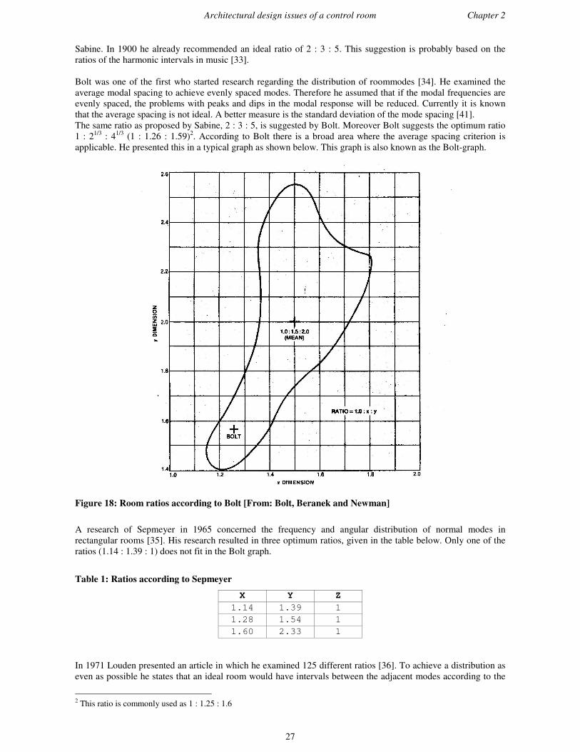
Sabine. In 1900 he already recommended an ideal ratio of 2 : 3 : 5. This suggestion is probably based on theratios of the harmonic intervals in music [33].
Bolt was one of the first who started research regarding the distribution of roommodes [34]. He examined theaverage modal spacing to achieve evenly spaced modes. Therefore he assumed that if the modal frequencies areevenly spaced, the problems with peaks and dips in the modal response will be reduced. Currently it is knownthat the average spacing is not ideal. A better measure is the standard deviation of the mode spacing [41].The same ratio as proposed by Sabine, 2 : 3 : 5, is suggested by Bolt. Moreover Bolt suggests the optimum ratio1 : 21/3 : 41/3 (1 : 1.26 : 1.59)2. According to Bolt there is a broad area where the average spacing criterion isapplicable. He presented this in a typical graph as shown below. This graph is also known as the Bolt-graph.
Figure 18: Room ratios according to Bolt [From: Bolt, Beranek and Newman]
A research of Sepmeyer in 1965 concerned the frequency and angular distribution of normal modes inrectangular rooms [35]. His research resulted in three optimum ratios, given in the table below. Only one of theratios (1.14 : 1.39 : 1) does not fit in the Bolt graph.
Table 1: Ratios according to Sepmeyer
X Y Z1.14 1.39 11.28 1.54 11.60 2.33 1
In 1971 Louden presented an article in which he examined 125 different ratios [36]. To achieve a distribution aseven as possible he states that an ideal room would have intervals between the adjacent modes according to the
2 This ratio is commonly used as 1 : 1.25 : 1.6
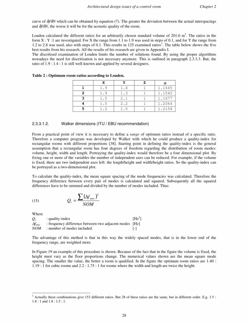
Architectural design issues of a control room Chapter 2
28
curve of δf/δN which can be obtained by equation (7). The greater the deviation between the actual interspacingsand δf/δN, the worse it will be for the acoustic quality of the room.
Louden calculated the different ratios for an arbitrarily chosen standard volume of 201.6 m3. The ratios in theform X : Y :1 are investigated. For X the range from 1.1 to 1.9 was used in steps of 0.1, and for Y the range from1.2 to 2.8 was used, also with steps of 0.1. This results in 125 examined ratios3. The table below shows the fivebest results from his research. All the results of his research are given in Appendix I.The discritised examination of Louden limits the number of solutions found. By using the proper algorithmsnowadays the need for discritisation is not necessary anymore. This is outlined in paragraph 2.3.3.3. But, theratio of 1.9 : 1.4 : 1 is still well-known and applied by several designers.
Table 2 : Optimum room ratios according to Louden.
X Y Z σσ1 1.9 1.4 1 1.14452 1.9 1.3 1 1.15423 1.5 2.1 1 1.16774 1.5 2.2 1 1.20645 1.2 1.5 1 1.2158
2.3.3.1.2. Walker dimensions (ITU / EBU recommendation)
From a practical point of view it is necessary to define a range of optimum ratios instead of a specific ratio.Therefore a computer program was developed by Walker with which he could produce a quality-index forrectangular rooms with different proportions [38]. Starting point in defining the quality-index is the generalassumption that a rectangular room has four degrees of freedom regarding the distribution of room modes:volume, height, width and length. Portraying the quality-index would therefore be a four dimensional plot. Byfixing one or more of the variables the number of independent axes can be reduced. For example, if the volumeis fixed, there are two independent axes left: the length/height and width/height ratios. So the quality-index canbe portrayed as a two-dimensional plot.
To calculate the quality-index, the mean square spacing of the mode frequencies was calculated. Therefore thefrequency difference between every pair of modes is calculated and squared. Subsequently all the squareddifferences have to be summed and divided by the number of modes included. Thus:
(15) ( )NOM
fQ nms
i∑ ∆
=2
WhereQi : quality-index [Hz2]∆fnms : frequency difference between two adjacent modes [Hz]NOM : number of modes included [-]
The advantage of this method is that in this way the widely spaced modes, that is in the lower end of thefrequency range, are weighted more.
In Figure 19 an example of this procedure is shown. Because of the fact that in the figure the volume is fixed, theheight must vary as the floor proportions change. The numerical values shown are the mean square modespacing. The smaller the value, the better a room is qualified. In the figure the optimum room ratios are 1.40 :1.19 : 1 for cubic rooms and 2.2 : 1.75 : 1 for rooms where the width and length are twice the height.
3 Actually these combinations give 153 different ratios. But 28 of these ratios are the same, but in different order. E.g. 1.5 :1.8 : 1 and 1.8 : 1.5 : 1.
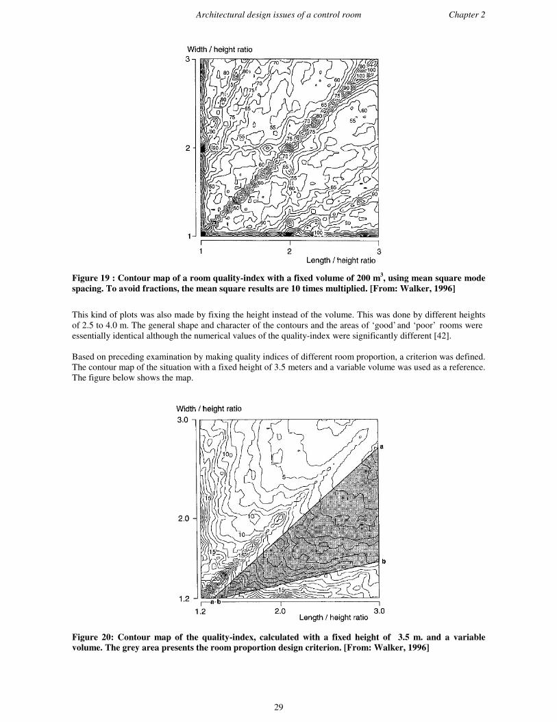
Architectural design issues of a control room Chapter 2
29
Figure 19 : Contour map of a room quality-index with a fixed volume of 200 m3, using mean square modespacing. To avoid fractions, the mean square results are 10 times multiplied. [From: Walker, 1996]
This kind of plots was also made by fixing the height instead of the volume. This was done by different heightsof 2.5 to 4.0 m. The general shape and character of the contours and the areas of ‘good’ and ‘poor’ rooms wereessentially identical although the numerical values of the quality-index were significantly different [42].
Based on preceding examination by making quality indices of different room proportion, a criterion was defined.The contour map of the situation with a fixed height of 3.5 meters and a variable volume was used as a reference.The figure below shows the map.
Figure 20: Contour map of the quality-index, calculated with a fixed height of 3.5 m. and a variablevolume. The grey area presents the room proportion design criterion. [From: Walker, 1996]

Architectural design issues of a control room Chapter 2
30
As the figure shows there is a large area with ‘better’ proportional ratios. By defining this area the roomproportions are no longer restricted to a certain golden ratio, which enables the designer in some situations towork much more efficient. I.e. with a range of room proportions the volume might be used much moreefficiently.
The lower limit for the length-to-width ratio, wl
, has a value of 1.1. This is indicated with the line a-a in Figure
20. This can be rewritten in the following formula, which presents the lower limit of the criterion:
(16) 1.1≥wl
or 1.1hw
hl ≥
where:l : length [m]w : width [m]h : height [m]
The upper limit for the length-to-height ratio, hl
, is altered to the line b-b in Figure 20. The equation of line b-b
is:
(17) 45.4 −=hw
hl
The new criterion which can be used for the room dimensions of an acoustically small room can now be definedas [38]:
(18) 45.41.1 −≤≤hw
hl
hw
with hl 3< and hw 3<
As can be seen from the formula and Figure 20 a wide range of room proportions without unjustified exclusionzones is permitted. Because in most cases the height is the smallest dimension, the criterion is on the essentialpractical limitation of a fixed height and a variable volume. Because the numerical values are weakly dependenton the room height, the criterion can be used for all reasonable room heights [42].
Moreover, the criterion is taken over by the European Broadcasting Union (EBU), for which the work wasoriginally carried out, and the International Telecommunication Union (ITU) in their recommendations forlistening rooms [38] [39]. The EBU and ITU remark in their recommendations that the ratios of l, w and h shouldbe avoided if they are within 5% of integer values of each other, because this increases the chance of theoccurrence of modes. At the moment most designers use the criterion in their first design approach.
2.3.3.2. Bonello criterion
In 1981 Bonello presented an article in which he proposed a criterion for the distribution of normal modes in aroom [29]. He calculated the first 48 modes according to the Rayleigh equation. (Eq. (5)) Subsequently thefrequency spectrum was divided in 1/3-octaves intervals and the number of modes in each interval was counted.The assumption that the ear is unable to discriminate modes within an interval, but only observes the sum of thetotal sound energy received in that band makes it plausible to count the number of modes. Finally, a 1/3-octavebandwidth is used. The reason to use a relative instead of an absolute bandwidth is because of the logarithmiccharacteristic of the ear [29].
As been stated in paragraph 2.3.3.1, the sound pressure of the different types of modes relative to each other isdifferent. Therefore it can be argued to weight the different modes. Moreover it can be argued to take intoaccount the loudness of each band due to the ear sensitivity. Because it is not easy to know the intensity of anaxial, tangential or oblique mode beforehand, i.e. among others the number of reflections they had is ofimportance, it is preferred by Bonello to suppose an ‘equal energy’ concept. [37]
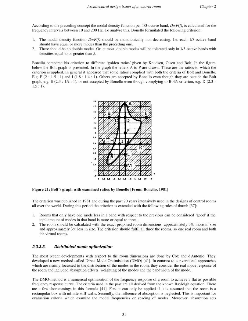
Architectural design issues of a control room Chapter 2
31
According to the preceding concept the modal density function per 1/3-octave band, D=F(f), is calculated for thefrequency intervals between 10 and 200 Hz. To analyse this, Bonello formulated the following criterion:
1. The modal density function D=F(f) should be monotonically non-decreasing. I.e. each 1/3-octave bandshould have equal or more modes than the preceding one.
2. There should be no double modes. Or, at most, double modes will be tolerated only in 1/3-octave bands withdensities equal to or greater than 5.
Bonello compared his criterion to different ‘golden ratios’ given by Knudsen, Olsen and Bolt. In the figurebelow the Bolt graph is presented. In the graph the letters A to P are drawn. These are the ratios to which thecriterion is applied. In general it appeared that some ratios complied with both the criteria of Bolt and Bonello.E.g. F (2 : 1.5 : 1) and I (1.8 : 1.4 : 1). Others are accepted by Bonello even though they are outside the Boltgraph, e.g. E (2.3 : 1.9 : 1), or not accepted by Bonello even though complying to Bolt’s criterion, e.g. D (2.3 :1.5 : 1).
Figure 21: Bolt’s graph with examined ratios by Bonello [From: Bonello, 1981]
The criterion was published in 1981 and during the past 20 years intensively used in the designs of control roomsall over the world. During this period the criterion is extended with the following rules of thumb [37]:
1. Rooms that only have one mode less in a band with respect to the previous can be considered ‘good’ if thetotal amount of modes in that band is more or equal to three.
2. The room should be calculated with the exact proposed room dimensions, approximately 3% more in sizeand approximately 3% less in size. The criterion should fulfil all three the rooms, so one real room and boththe virtual rooms.
2.3.3.3. Distributed mode optimization
The most recent developments with respect to the room dimensions are done by Cox and d’Antonio. Theydeveloped a new method called Direct Mode Optimisation (DMO) [41]. In contrast to conventional approacheswhich are mainly focussed to the distribution of the modes in the room, they consider the real mode response ofthe room and included absorption effects, weighting of the modes and the bandwidth of the mode.
The DMO-method is a numerical optimisation of the frequency response of a room to achieve a flat as possiblefrequency response curve. The criteria used in the past are all derived from the known Rayleigh equation. Thereare a few shortcomings in this formula [41]. First it can only be applied if it is assumed that the room is arectangular box with infinite stiff walls. Secondly, the influence of absorption is neglected. This is important forevaluation criteria which examine the modal frequencies or spacing of modes. Moreover, absorption acts

Architectural design issues of a control room Chapter 2
32
different on axial, tangential and oblique modes. The magnitude of an axial mode is the greatest, but it will bedamped least regarding the tangential and oblique modes. Therefore weighting the type of mode is advocated. Inthe past this was never done, although Gilford discussed the prominence of axial modes regarding speech studios[42].
To avoid these shortcomings, the DMO-method uses algorithms which take absorption and impedance of thesurfaces into account. Furthermore, the type of mode is discounted. Because the model acts directly on the modalresponse of the room, a criterion based on mode spacing is no longer required. However some kind of anevaluation criterion is required. This criterion can be based on the modal response of the room, and therefore itwill be easier to relate it to the human perception [41].
To achieve a flat power spectrum two models have been considered to predict the modal response. A frequencybased modal decomposition model and a time based image source model. Starting point in both models is a roomwith an omni-directional microphone in one of the corners and a loudspeaker in the opposite corner.
2.3.3.3.1. Modal decomposition model
This frequency based model is applicable when the impedance of the borders is large and real. When a room isconsidered as a second order resonator (see also paragraph 2.3.1), the pressure p(r,ω) at position r(x,y,z) in theroom, due to a source at r0(x0,y0,z0) with an angular frequency ω is given by :
(19) ( )
( )∑∑∑∞ ∞ ∞
−−=
x y zn n n rrn jrrA
rpωδωωω
ω ω
2,
),(22
0
where δr presents a damping constant and Aω a function of the position of the source and receiver and thefrequency.
Formula (19) gives the frequency response of the transmission path between the source and the receiver. Thus itenables us to determine the pressure in a room at every position, at any frequency in the room.
2.3.3.3.2. Image Source model
The image source model is much faster than the modal decomposition model for box-shaped rooms. Once theenergy impulse response is obtained, the frequency response is formed by a Fourier Transformation. Thereforethe following relation is valid:
(20) ∑∑∑∑∞ ∞ ∞
=
=x y zn n n i in
in dRrrtE
2
12,
2,0
1),,(
Where
E(t,r,r0) : energy impulse responseR2
n,i : surface reflection factord2
n,i : distance between source and surface
The disadvantage of this method is that the accuracy of the calculation decreases with an increasing absorptionfactor because then the image source can no longer be seen as a pure point source. Moreover, the accuracydecreases with increased order of the reflection because the higher the order of the reflection the less highfrequent energy is in the wave.
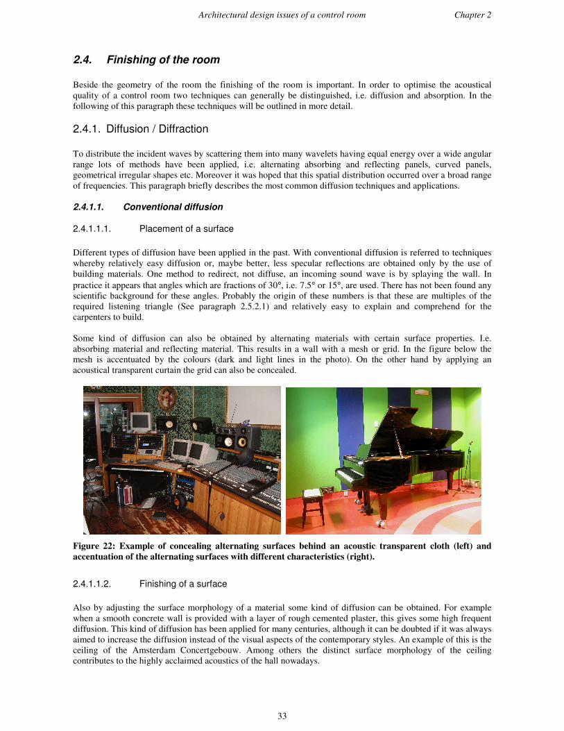
Architectural design issues of a control room Chapter 2
33
2.4. Finishing of the room
Beside the geometry of the room the finishing of the room is important. In order to optimise the acousticalquality of a control room two techniques can generally be distinguished, i.e. diffusion and absorption. In thefollowing of this paragraph these techniques will be outlined in more detail.
2.4.1. Diffusion / Diffraction
To distribute the incident waves by scattering them into many wavelets having equal energy over a wide angularrange lots of methods have been applied, i.e. alternating absorbing and reflecting panels, curved panels,geometrical irregular shapes etc. Moreover it was hoped that this spatial distribution occurred over a broad rangeof frequencies. This paragraph briefly describes the most common diffusion techniques and applications.
2.4.1.1. Conventional diffusion
2.4.1.1.1. Placement of a surface
Different types of diffusion have been applied in the past. With conventional diffusion is referred to techniqueswhereby relatively easy diffusion or, maybe better, less specular reflections are obtained only by the use ofbuilding materials. One method to redirect, not diffuse, an incoming sound wave is by splaying the wall. Inpractice it appears that angles which are fractions of 30°, i.e. 7.5° or 15°, are used. There has not been found anyscientific background for these angles. Probably the origin of these numbers is that these are multiples of therequired listening triangle (See paragraph 2.5.2.1) and relatively easy to explain and comprehend for thecarpenters to build.
Some kind of diffusion can also be obtained by alternating materials with certain surface properties. I.e.absorbing material and reflecting material. This results in a wall with a mesh or grid. In the figure below themesh is accentuated by the colours (dark and light lines in the photo). On the other hand by applying anacoustical transparent curtain the grid can also be concealed.
Figure 22: Example of concealing alternating surfaces behind an acoustic transparent cloth (left) andaccentuation of the alternating surfaces with different characteristics (right).
2.4.1.1.2. Finishing of a surface
Also by adjusting the surface morphology of a material some kind of diffusion can be obtained. For examplewhen a smooth concrete wall is provided with a layer of rough cemented plaster, this gives some high frequentdiffusion. This kind of diffusion has been applied for many centuries, although it can be doubted if it was alwaysaimed to increase the diffusion instead of the visual aspects of the contemporary styles. An example of this is theceiling of the Amsterdam Concertgebouw. Among others the distinct surface morphology of the ceilingcontributes to the highly acclaimed acoustics of the hall nowadays.
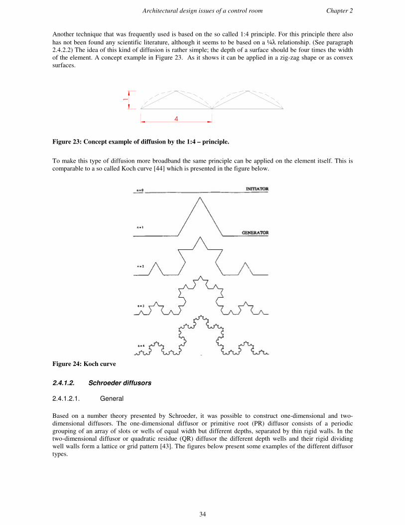
Architectural design issues of a control room Chapter 2
34
Another technique that was frequently used is based on the so called 1:4 principle. For this principle there alsohas not been found any scientific literature, although it seems to be based on a ¼λ relationship. (See paragraph2.4.2.2) The idea of this kind of diffusion is rather simple; the depth of a surface should be four times the widthof the element. A concept example in Figure 23. As it shows it can be applied in a zig-zag shape or as convexsurfaces.
14
Figure 23: Concept example of diffusion by the 1:4 – principle.
To make this type of diffusion more broadband the same principle can be applied on the element itself. This iscomparable to a so called Koch curve [44] which is presented in the figure below.
Figure 24: Koch curve
2.4.1.2. Schroeder diffusors
2.4.1.2.1. General
Based on a number theory presented by Schroeder, it was possible to construct one-dimensional and two-dimensional diffusors. The one-dimensional diffusor or primitive root (PR) diffusor consists of a periodicgrouping of an array of slots or wells of equal width but different depths, separated by thin rigid walls. In thetwo-dimensional diffusor or quadratic residue (QR) diffusor the different depth wells and their rigid dividingwell walls form a lattice or grid pattern [43]. The figures below present some examples of the different diffusortypes.

Architectural design issues of a control room Chapter 2
35
(a) (b) (c)
Figure 25: 1D diffusor (a, b), 2D diffusor (c) [Courtesy: RPG diffusor systems]
The well depths are determined by mathematical sequences which have the critical property that the FourierTransform of the exponentiated sequence values has a constant magnitude. The QR sequence satisfies thisrequirement exactly at the design frequency f0. The PR sequence provides an approximate constant magnitudeover the scattering bandwidth. In appendix II the algorithms for a Schroeder diffusor are given.
Schroeder diffusors are widely used in concert halls, theatres and control rooms. Besides their diffusing quality,it also appeared that they absorb, mainly below the design frequency of the diffusors, considerably [45]. Amongothers Fujiwara, Kuttruff and Wu have performed intensive research on this subject. Kuttruff’s research [46]revealed that due to a strong interaction between each of the elements, the wells are tuned for a specificresonance frequency. This results in an air flow at the mouth of a well with a higher velocity than the partialvelocities in the direct sound field. Hence there will be pressure differences between the slots. As the equalisingflows lead to a much higher energy loss than is effected by channels of equal depth, this introduces extra lowfrequent absorption.
Fujiwara’s examination [47] showed that also a poor construction of the diffusor contributes to extra absorptionof the diffusor in the lower frequencies. The back space behind the well bottom and small gaps between thecomponents increase the low frequency absorption. Filling the back space with a material with a higherimpedance as the construction material of the diffusor bottom and painting the elements appeared to be veryeffective regarding the reduction of the low frequency absorption of the diffusor.
In a research of Wu [48] this low frequency absorption is used to create a profiled structure to improve the lowfrequency absorption. Eventually it appeared that applying a perforated element as a well bottom in an elementwhich consists of wells with an equal depth, have the best low frequency absorbing characteristics. An additionalbenefit of this method is that there is a possibility to fine-tune the corresponding space.
2.4.2. Absorption
As has been outlined in chapter 1 reflections can introduce some kind of distortion on the sound image. In thisparagraph one of the mechanisms to control the reflections, i.e. attenuation, is discussed. To attenuate disturbingreflections, the walls are treated with absorption. The attenuation of the reflections by absorption characterisesitself by the fact that it transfers the energy into heat at a specific frequency or frequency range.
Different types of absorbers can be distinguished, each with their own characteristics, benefits and drawbacks.Generally we distinguish two main groups, i.e. the porous absorbers and the resonators. In the following thesewill be discussed in higher detail.
2.4.2.1. Porous absorbers
A porous absorber is basically a material with an open pore structure, e.g. mineral wool. The incoming acousticenergy is transferred into heat by the friction the wave goes through by the molecules of the material. From thegeneral wave equation it can be derived that the maximum velocity of a standing wave occurs at ¼λ and ¾λ infront of a rigid wall. Therefore the thickness of the material is very important regarding the effectivity of theabsorber.

Architectural design issues of a control room Chapter 2
36
(a) (b)
Figure 26 : Application principle of a porous absorber.
The frequency at which a porous absorber is most effective, f0 [Hz], can be calculated with
(17) dc
f40 =
where c is the velocity of sound in [m/s] d is the thickness of the material in m.
Porous absorbers are mainly used for high frequency absorption. The presence of an air space between thematerial and a rigid wall (Figure 26 (b)) results in an increase of absorption at low frequencies. An increase inthe air space is accompanied by a shift of the maximum absorption towards the low frequencies and to anincrease in the maximum coefficient [50]. The figure below confirms this by measurements of Mankovsky.
Figure 27 : Frequency characteristics of the absorption coefficient for a layer of plaster at differentdistances (14; 5; 0.5; and 0 mm from a rigid wall). [From: Mankovsky, 1971]
Furthermore, eq. (17) shows that in case of applying a larger thickness, the absorber can also act as a lowfrequency absorber. A porous low frequent absorber is also known as a bass trap. In control rooms this type oflow frequency absorption is quite common to suppress the eigenmodes. They are mainly placed in the corners ofthe room because they are there most effective.For normal incidence the absorption coefficient of a porous layer can be obtained by [51]:
(18) ( )21
4σσα
+=
Where σ [-] represents the porosity factor of a certain material.Table 3 presents a few materials with their porosity factors.

Architectural design issues of a control room Chapter 2
37
Table 3 : Range of measured porosity factors [After: Cremer and Müller, 1982]
Material Porosityfactor (σσ)
Mineral wool 0.94 - 0.98Felt 0.83 - 0.95Fiberplates 0.65 - 0.80Porous plaster 0.60 - 0.65Ceramic filter 0.33 - 0.42Brick 0.25 - 0.30Firebrick 0.15 - 0.35Sandstone 0.02 - 0.06Marble about 0.005
2.4.2.2. Resonators
Another type of absorption are the resonators. Resonators are often presented as mass-spring systems. Generallytwo types of resonators can be distinguished, the slit- or Helmholtz resonators and the panel resonators. Themain characteristic of the resonators is that they can be tuned to a specific frequency, the resonance frequency f0,at which they are most effective.
2.4.2.2.1. Slit absorbers
The mass-spring system of a slit absorber consists of the air in the neck of the resonator which represents themass and the air in the volume behind which represents the spring of the system. In the figure below theprinciple of a slit absorber is drawn.
V
bA
Mass
Figure 28 : Principle application of a slit absorber.
The mass of the neck and the compliance with the volume behind is the resonating system of a slit absorber. Inessence this type of resonator is based on the reduction of energy due to the decrease in the particle velocity ofthe sound energy in the air.When the internal resistance of the Helmholtz-resonator is low, the effective bandwidth of the absorber is verysmall. Thus Q-factor of the absorber is high [49].
Already in 1896 the resonance frequency of a Helmholtz resonator with a cylindrical neck was defined by LordRayleigh. He found that the resonance frequency for such an absorber can be found according to the relation:

Architectural design issues of a control room Chapter 2
38
(19) VlAc
f'20 π
= with2
'r
llπ+=
Wherec : velocity of sound [m/s]A : cross sectional area neck [m2]l’ : effective length of the neck [m]l : length of the neck [m]r : radius of the neck [m]V : volume behind the neck [m3]
r
l
A
Figure 29 : Principle of a slit absorber with a cylindrical neck.
Almost half a century later in 1940 the general formula for slit absorbers was derived by Peterson:
(20)
'ln12,122
0
0
Afb
cbl
bcf
⋅
⋅⋅
+⋅⋅+=
πππ
Where
b : width of the slit [m2]l : length of the neck [m2]A’ : cross sectional area behind the neck [m2]
l
b
A’
Figure 30 : Principle of a slit resonator.
The bandwidth ∆fH of a slit absorber is defined as the frequency range between frequencies whereby the soundpressure level is 3 dB down with respect to the design frequency f0 :
(21) 2
438cVf
f H
π=∆

Architectural design issues of a control room Chapter 2
39
One of the advantages of this type of absorber is that they can be applied over a very large range of frequencies,although it has to be remarked that in some cases the elements can become quite large. Furthermore the slitabsorber has the advantage that it can be tuned afterwards. For example when a control room is finished and dueto construction errors there are some acoustic distortions, it is possible to tune the absorber afterwards. Thereforea microphone is placed in the absorber. Subsequently the width of the slit is adjusted until the desired resonancefrequency is obtained.
In the table below an example is given of an absorber with cross sectional area behind the neck A’ of 0.005 cm2,length of the neck l is 0.05 m and the volume of the resonator V is 0.02 m3. For this element a frequency range of160 Hz can be realised by varying the width b from 0.5 to 3.0 cm.
Table 4 : Example of possible tuning frequencies for a slit resonator with the fixed parameters A' = 0.005m2, l = 0.05m, V = 0.02 m3.
b [cm] f0 [Hz] ∆∆f [Hz]0.5 373.0 236.6
1.0 427.1 407.81.5 462.5 557.62.0 489.7 700.82.5 513.0 843.83.0 533.9 989.9
On the other hand, the possibility of tuning the resonators afterwards is also a drawback of the Helmholtzresonator. Because the tuning is so critical, small deviations during the construction can have large effects on thequality of the resonator. Therefore a slit absorber always has to be tuned in situ, which is a relatively timeconsuming matter. Furthermore the slit absorber is a so called active absorber which has an open connectionbetween the resonating volume and the air in the room. This results in non-linear distortion of the resonator.Normally this distortion is negligible. Although in critical listening environments, especially near loudspeakers,this interaction can distort the sound image perceived by the engineer. This is one of the main reasons manycontrol room designers refuse to apply slit absorbers in their designs.
2.4.2.2.2. Panel absorbers
In contradiction to a slit absorber, a panel absorber is a selective low frequency absorber. In practice the panelabsorber is most commonly used. The main advantage of the panel absorber is that many of those can be foundin every room. For instance, a ceiling or a floating floor are examples of mechanisms which also act as panelabsorbers.A panel absorber can also be presented as a mass-spring system. In this case the mass is not an air column butthe mass of the panel itself. The spring is given by the coupling, i.e. the air space, between the panel and the wallbehind, and the stuffing of the airspace between. The figure below presents a principle application of a panelabsorber.
Figure 31 : Principle application of a panel absorber.
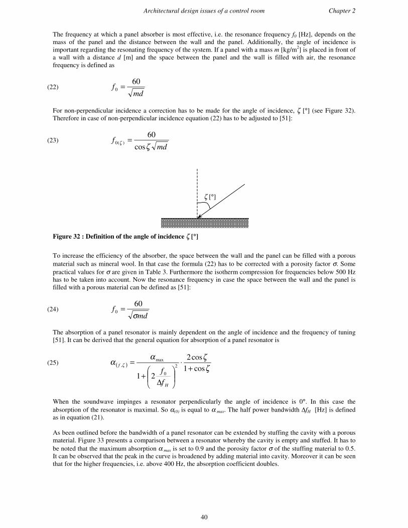
Architectural design issues of a control room Chapter 2
40
The frequency at which a panel absorber is most effective, i.e. the resonance frequency f0 [Hz], depends on themass of the panel and the distance between the wall and the panel. Additionally, the angle of incidence isimportant regarding the resonating frequency of the system. If a panel with a mass m [kg/m2] is placed in front ofa wall with a distance d [m] and the space between the panel and the wall is filled with air, the resonancefrequency is defined as
(22) md
f60
0 =
For non-perpendicular incidence a correction has to be made for the angle of incidence, ζ [°] (see Figure 32).Therefore in case of non-perpendicular incidence equation (22) has to be adjusted to [51]:
(23) md
fζζ
cos
60)(0 =
ζ [°]
Figure 32 : Definition of the angle of incidence ζζ [°°]
To increase the efficiency of the absorber, the space between the wall and the panel can be filled with a porousmaterial such as mineral wool. In that case the formula (22) has to be corrected with a porosity factor σ. Somepractical values for σ are given in Table 3. Furthermore the isotherm compression for frequencies below 500 Hzhas to be taken into account. Now the resonance frequency in case the space between the wall and the panel isfilled with a porous material can be defined as [51]:
(24) md
fσ60
0 =
The absorption of a panel resonator is mainly dependent on the angle of incidence and the frequency of tuning[51]. It can be derived that the general equation for absorption of a panel resonator is
(25) ( ) ζζα
α ζ cos1cos2
212
0
max, +
⋅
∆
+
=
H
f
ff
When the soundwave impinges a resonator perpendicularly the angle of incidence is 0°. In this case theabsorption of the resonator is maximal. So α(0) is equal to α max. The half power bandwidth ∆fH [Hz] is definedas in equation (21). As been outlined before the bandwidth of a panel resonator can be extended by stuffing the cavity with a porousmaterial. Figure 33 presents a comparison between a resonator whereby the cavity is empty and stuffed. It has tobe noted that the maximum absorption α max is set to 0.9 and the porosity factor σ of the stuffing material to 0.5.It can be observed that the peak in the curve is broadened by adding material into cavity. Moreover it can be seenthat for the higher frequencies, i.e. above 400 Hz, the absorption coefficient doubles.

Architectural design issues of a control room Chapter 2
41
0,0
0,1
0,2
0,3
0,4
0,5
0,6
0,7
0,8
0,9
1,0
0 50 100 150 200 250 300 350 400 450 500
Frequency [Hz]
α [−
]α
[−]
Cavity Stuffed cavity
Figure 33 : Effect of adding material in the cavity on the bandwidth of the absorber. (αα max = 0.9; σσ = 0.5)
2.4.2.2.3. ¼λ-resonators
The sound energy emitted by a loudspeaker travels from the loudspeaker to the engineer and continues to therear wall where it is reflected back to the engineer. This reflection can be detrimental to the sound imageperceived by the engineer because of the interference between the direct sound and the reflected sound.Absorbing this high level reflection with a panel absorber might be quite ineffective because of the fact that apanel absorber needs a few cycles to be most effective [52]. In order to maintain the energy but omit thedestructive reflection a ¼λ-resonator can be applied. A ¼λ-resonator is a large well, e.g. behind a wall, whereby the energy will be released ½λ later in time relativeto when it should be reflected by the wall. As a result the destructive interference at the design position will bereduced. The frequency at which the resonator will be effective depends on the length of the well. E.g. aresonator which is effective at 100 Hz has to have a length of 0.85 meters.
d = ¼λ l = d
Figure 34 : Concept of a ¼λλ-resonator
The ¼λ-resonator has a few drawbacks. Like the slit- and panel- absorber, the effectivity of a ¼λ resonator istemperature dependent and, because they are reactive resonators, they can cause non-linear distortion. The maindisadvantage of this absorber is that it is only effective at a specific position because the specific resonancefrequency at which it is designed is based on the distance between a certain position in the room and the wall.
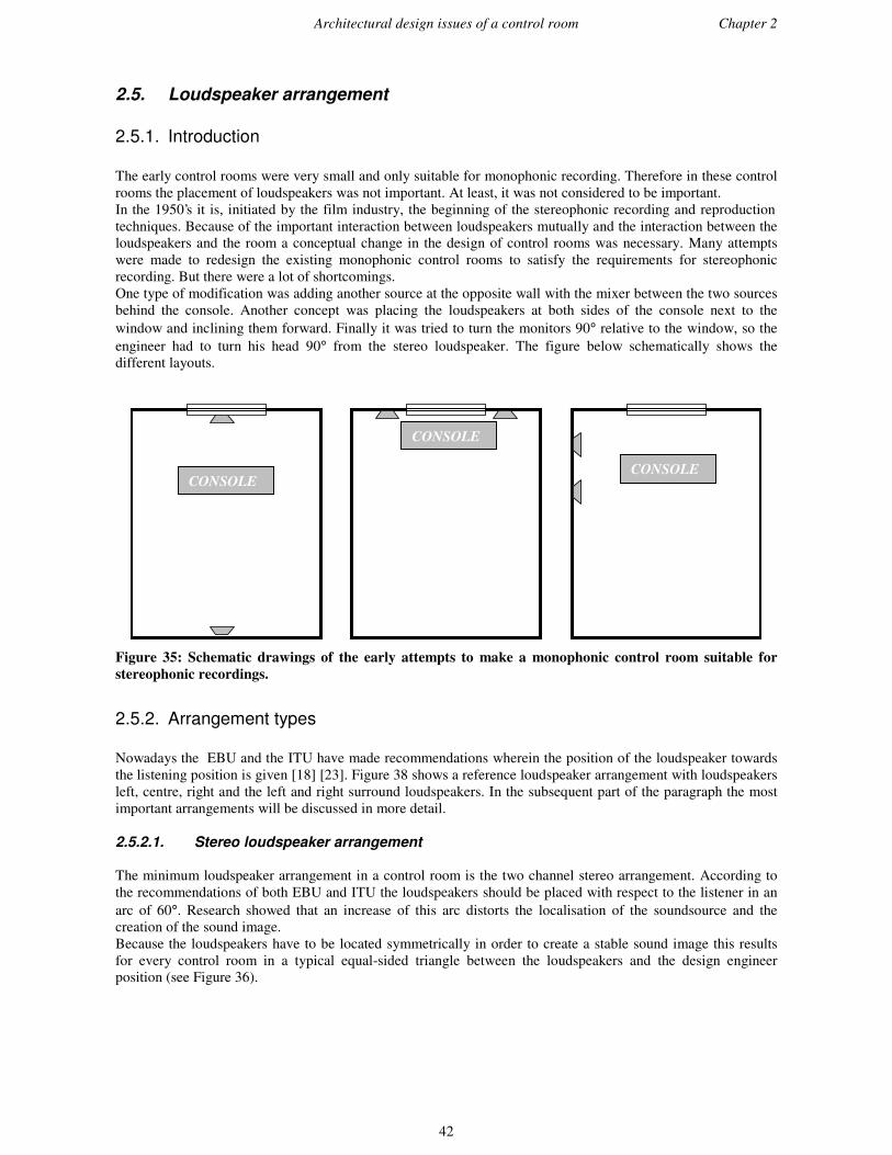
Architectural design issues of a control room Chapter 2
42
2.5. Loudspeaker arrangement
2.5.1. Introduction
The early control rooms were very small and only suitable for monophonic recording. Therefore in these controlrooms the placement of loudspeakers was not important. At least, it was not considered to be important.In the 1950’s it is, initiated by the film industry, the beginning of the stereophonic recording and reproductiontechniques. Because of the important interaction between loudspeakers mutually and the interaction between theloudspeakers and the room a conceptual change in the design of control rooms was necessary. Many attemptswere made to redesign the existing monophonic control rooms to satisfy the requirements for stereophonicrecording. But there were a lot of shortcomings.One type of modification was adding another source at the opposite wall with the mixer between the two sourcesbehind the console. Another concept was placing the loudspeakers at both sides of the console next to thewindow and inclining them forward. Finally it was tried to turn the monitors 90° relative to the window, so theengineer had to turn his head 90° from the stereo loudspeaker. The figure below schematically shows thedifferent layouts.
CONSOLE
CONSOLE
CONSOLE
Figure 35: Schematic drawings of the early attempts to make a monophonic control room suitable forstereophonic recordings.
2.5.2. Arrangement types
Nowadays the EBU and the ITU have made recommendations wherein the position of the loudspeaker towardsthe listening position is given [18] [23]. Figure 38 shows a reference loudspeaker arrangement with loudspeakersleft, centre, right and the left and right surround loudspeakers. In the subsequent part of the paragraph the mostimportant arrangements will be discussed in more detail.
2.5.2.1. Stereo loudspeaker arrangement
The minimum loudspeaker arrangement in a control room is the two channel stereo arrangement. According tothe recommendations of both EBU and ITU the loudspeakers should be placed with respect to the listener in anarc of 60°. Research showed that an increase of this arc distorts the localisation of the soundsource and thecreation of the sound image.Because the loudspeakers have to be located symmetrically in order to create a stable sound image this resultsfor every control room in a typical equal-sided triangle between the loudspeakers and the design engineerposition (see Figure 36).

Architectural design issues of a control room Chapter 2
43
A
Figure 36 : Example of the typical listening triangle. [Courtesy: Balster, 2001]
As can be seen in the figure above, the third corner of the triangle, indicated with an A, is behind the designedengineer position. This is a doubtful issue. There are designers who insist on having the triangle behind theengineer while in that situation most of the perceived sound is direct energy which is higher in level than thereflections. This should overcome problems like comb filtering or losing the definition in the sound image.
On the other hand there are designers who prefer to have the third corner at the engineer position. In chapter 1 itwas already revealed that time- and level differences between the loudspeakers are very important in theperception of the loudspeakers. The optimisation of the time and level differences in the given loudspeakerarrangement only works for the median plane between the loudspeakers. Thus, in case that there are morelisteners in the room, they should be positioned behind each other in a line so that they all can have a good soundimage. By level and time differences the optimum listening area can be enlarged. As Franssen [54] suggests, thelisteners should be placed behind the on-axis lines of the directed loudspeakers. (See Figure 37)
Figure 37: Loudspeaker configuration proposed by Franssen. [After: Franssen, 1962]
When people move to the right in this loudspeaker arrangement for instance, this implies an increase in levelfrom the right loudspeaker and a decrease of the left loudspeaker. On the other hand the time difference betweenthe loudspeakers increases. This should result in a more stable sound image.

Architectural design issues of a control room Chapter 2
44
100°100°
120°120°
60°
RL
LS
2 1C
B
1β
2β
RS
Figure 38: Loudspeaker arrangment according to ITU. [From: ITU 775-1, 1994]
Besides the angle between the loudspeaker and the engineer also the distance with reference to the listener has tobe determined. The EBU recommends a distance between the loudspeakers of 2.0 to 4.0 meters. Therefore thedistance perpendicular on the axis between the loudspeakers (h in Figure 39) should be 90% of the distancebetween the loudspeakers, so 1.8 to 3.6 meters.
h
Figure 39: Typical stereo listening arrangement. [From: EBU, 1997]
Table 5 shows the results of an investigation by Mäkivirta and Anet [53] in which they examined among othersthe in situ arrangements of loudspeakers in control rooms. As the table shows the results agree very well with theEBU and ITU recommendations. The average distance between the listener and the left and right channel withrespect to the listener in a stereo loudspeaker arrangement is 2.36 to 2.39 m. In the case of an extra centrespeaker the average is 2.66 meters.

Architectural design issues of a control room Chapter 2
45
Table 5 : Mean listening distances in meters of individual channels for left-right stereo rooms, left-center-right triplet rooms and five-channel full surround rooms. [After: Mäkivirta and Anet, 2001]
Channel StereoN = 79
L/C/R4
N =155-channel
N = 8Left 2.36 2.66 2.68
Center 2.66 2.71Right 2.39 2.66 2.71
Surround left 2.70Surround right 2.69
2.5.2.2. Multi channel loudspeaker arrangement
Based on the film industry, the multi-channel loudspeaker arrangement in control rooms has become moreimportant during the last 15 years. Companies like Dolby and Lucasfilm (THX) started with the application ofsurround sound. Later on also the music industry started producing surround sound products, however the mainapplication for surround sound applications is still the film industry.
Based on the necessity for surround sound the ITU and EBU have also set up recommendations for this type ofloudspeaker arrangements [19],[23]. As can be seen in Figure 40, the rear loudspeakers should be placed withinan arc of 100° to 120°. If there are more than two rear loudspeakers used, the loudspeakers should be placedsymmetrically and on equal distances between an arc of 60° to 150° [23].
150°
60°
LC
B
150°
60°
60°
R
LS 1 RS1
LS2 RS2
02
Figure 40: Loudspeaker arrangement if more than 2 rear loudspeakers are used [From: ITU 775-1, 1994]
4 L/C/R refers to Left – Center – Right loudspeakers. This extra center loudspeaker is obtained from the film industry whereit is used for dialogs.

Architectural design issues of a control room Chapter 2
46
As can be revealed from the figure above, the loudspeakers are placed in a circle. The radius of this circle isdetermined by the described equal-sided triangle in the previous paragraph about stereo loudspeakerarrangements. The placement of the front left and right loudspeaker is the most important for the creation of acorrect sound image. The rear ones are necessary for the ambience, surround or spatial impression.Although it is recommended to arrange all the speakers on a circle, as a consequence of the geometry of theroom it is sometimes impossible to arrange the loudspeakers on a circle. To overcome this problem it is generallyrecommended to insert a delay on the output of the different channels [19] [23]. As a result the speaker movesvirtually backwards with respect to optimised listening position. The length of the delays should be so long, thatthe loudspeakers again will be perceived as they were placed on a circle.Instead of virtually replacing the loudspeakers by adding a delay, this can also be accomplished by changing thebalance between the loudspeakers. For example a loudspeaker which is placed too far away from the circle couldbe increased in level whereby the speaker virtually moves towards the circle.
Although it is generally recommended to insert time delays if the speakers cannot be arranged on a circle, inactual practice it appeared that increasing the angle of the loudspeakers with respect to the centre plane showsbetter results than adding delays [52] [55].
2.5.2.3. Low frequency loudspeaker placement
In the past a lot of research has been performed regarding the placement of the low frequency loudspeaker. Asthis loudspeaker is effective in the lower part of the frequency spectrum, the subwoofers easily activate theeigenmodes in a room. Moreover the interactions of a room and loudspeaker is often the dominant factor in theperceived timbre, especially at low frequencies [56].
A recent examination [57] aimed at finding out how many subwoofers should be enough to have an equal aspossible frequency response in a 4 x 4 matrix. For this purpose a virtual rectangular room was used with infiniterigid walls. Based on measurements in a virtual and an actual room, it appeared that two loudspeakers placed onboth sides of the median plane should be a minimum but four, i.e. in the middle at each side of a rectangularroom, is given as a rule of thumb.
In actual practice it appears that the subwoofer is not used very frequently. Moreover, most of the time it is onlyused during the final listening tests of a recording, while during the mixing procedure only the satelliteloudspeakers are used. As the subwoofers are not used that often and keeping in mind that these are relativelyexpensive, it appears that in most cases people are satisfied with only one subwoofer.
In many cases this subwoofer is placed on the median plane, below the centre loudspeaker in front of theengineer. As the LF-loudspeaker easily activates roommodes, it is possible that the engineer is just located in anode of an axial mode which distorts the frequency response at the engineer position. Therefore it should bebetter to place a subwoofer off-axis with respect to the vertical median plane. When a subwoofer activates in thatsituation an axial roommode it will not be on the engineer position. It still might be possible however to have atangential mode at the engineer position, but this has a 3 dB lower level relative to an axial mode and is thereforeless detrimental.
2.5.2.4. Height of the loudspeakers
To avoid troublesome reflections from the console (see Figure 41), equipment racks etc. the height andcontorting of the loudspeakers is important. Therefore it is important to be fully aware of the way the reflectionsact in the room and consider these in the design.
Figure 41: Console reflection

Architectural design issues of a control room Chapter 2
47
To achieve optimum monitoring conditions it is generally recommended to locate the acoustical centre of theloudspeakers at ear height. Normally this is 1.2 m. The ITU recommends that the front loudspeakers should beplaced on ear height, while the rear speakers might be placed above this height. However, if the on-axis line hasto be directed towards the listener, the loudspeaker has to be tilted. The maximum tolerated tilt of the surroundloudspeakers recommended by the ITU is 15°.In contradiction, the EBU also allows tilting of the front loudspeakers, although they allow a maximum tilt of thefront loudspeakers of 10°.
2.5.3. Near field or wall mounted loudspeakers
One of the primer issues a designer has to deal with is the question whether the room gets near fieldloudspeakers, wall mounted loudspeakers or both. In the case of near field listening the engineer is able to judgethe recording more accurately because he is in the direct field of the sound. By using near field monitors theinteraction between the walls is very important because of the speaker boundary interference problems. On thecontrary, when using the wall mounted loudspeakers, the interaction between the room and the loudspeaker isless important regarding the speaker boundary interference but the loading of the loudspeakers by the wall isimportant, specifically at low frequencies.
Figure 42 : Example of a control room suited for near field monitoring and using wall mountedloudspeakers.
In actual practice it appeared that in most cases both near field and wall mounted loudspeakers are used. Only ifthe room is too small only near field loudspeakers are used. Therefore in general it can be stated that when acontrol room will be equipped with wall mounted loudspeakers the design should be optimised for these.

Design philosophies Chapter 3
48
3. Design philosophies
3.1. Introduction
Over the years a number of different approaches in designing control rooms have been proposed. The earlycontrol rooms were aimed to be a representation of the average final listening environment. When thestereophonic reproduction started also the problems with the early reflections became apparent. To control theseearly reflections a lot of absorption was applied in the control rooms which resulted in acoustically ‘dead’ rooms.Around 1980 there were concepts with a less uniform distribution of the acoustical materials. At present, at thebeginning of the new millennium the control rooms have to be suited more often for multi-channelreproductions.This chapter is aimed to give an overview of the different approaches over the years. Some of the approaches arestill applied, or improved designs have been derived from the original approaches. The most importantapproaches will be discussed in greater detail.
3.2. Horn coupled soffits – Putnam (1960)
The early control rooms were very small and only suitable for monophonic recording. Therefore in these controlrooms the placement of loudspeakers was not important. At least, it was not considered to be important. In theearly days a few attempts were made to find out which loudspeaker placement was the best for stereophonicsound reproduction, as discussed in paragraph 2.5.1.
Being aware of the problems related to stereophonic sound reproduction, Putnam was one of the first who triedto develop a concept for the design of control rooms suited for stereophonic sound reproduction. Essentially, hisconcept is based on the integration of the loudspeakers with the control room layout. In 1959 he started a newdirection with the United Recording Corporation studios in Hollywood [58]. Here the monitor loudspeakerswere placed under a soffit to accommodate the transition from monaural to stereophonic recording. This resultedin an increase of the radiation efficiency of the loudspeakers.
Figure 43 : Loudspeaker lay out of the United Recording Corporation control room. [From: Putnam,1960]
Later, in 1981, the concept was further evolved. To attain a larger listening area he moved the console back fromthe traditional location against the observation window (see Figure 44).The movement of the console backwards introduces low frequency anomalies and a new travelling path underthe console. Putnam realised this and in order to solve these problems he emphasised on the placement of the
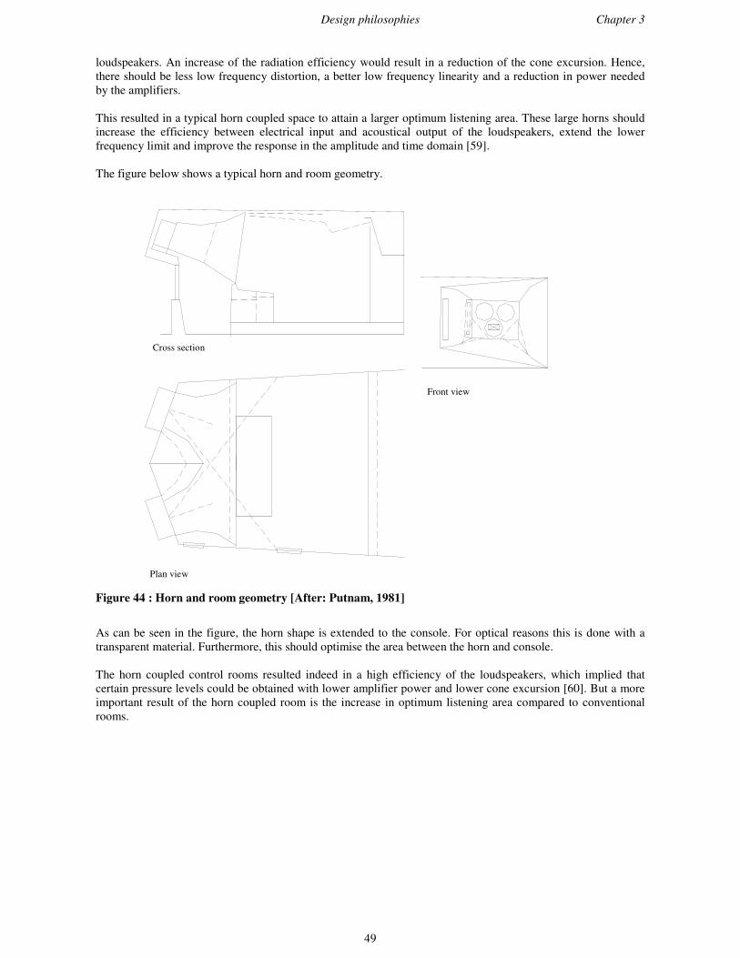
Design philosophies Chapter 3
49
loudspeakers. An increase of the radiation efficiency would result in a reduction of the cone excursion. Hence,there should be less low frequency distortion, a better low frequency linearity and a reduction in power neededby the amplifiers.
This resulted in a typical horn coupled space to attain a larger optimum listening area. These large horns shouldincrease the efficiency between electrical input and acoustical output of the loudspeakers, extend the lowerfrequency limit and improve the response in the amplitude and time domain [59].
The figure below shows a typical horn and room geometry.
Cross section
Plan view
Front view
Figure 44 : Horn and room geometry [After: Putnam, 1981]
As can be seen in the figure, the horn shape is extended to the console. For optical reasons this is done with atransparent material. Furthermore, this should optimise the area between the horn and console.
The horn coupled control rooms resulted indeed in a high efficiency of the loudspeakers, which implied thatcertain pressure levels could be obtained with lower amplifier power and lower cone excursion [60]. But a moreimportant result of the horn coupled room is the increase in optimum listening area compared to conventionalrooms.

Design philosophies Chapter 3
50
Figure 45 : Two views of the integrated horn according to Putnam’s approach. Compared to Figure 43 theevolution of the concept is clearly visible. (United/Western Studios) [From: Putnam, 1981]
3.3. Inert room approach – Veale (1973)
One of the first who directly linked psychoacoustics to the design of a control room is Edward J. Veale. In 1973he presented an article in which he emphasised the importance of a well built up sound image in our brains [61].Veale’s approach is to create an inert room. In this type of room the sound of the loudspeaker is interpreted bythe ear without any influence of the room.
3.3.1. Design criterion
According to Veale the objective in the acoustic design of a control room should be to create an inert room. Thisimplies that the room acoustics should be designed so that the information radiated by the loudspeaker isinterpreted by the sensory system of the listener in such a way that no addition or subtraction is made by theroom to the sound picture [61]. In this respect, consideration has to be given to the auditory system and theacoustic materials.
3.3.1.1. Auditory system
In addition to the direct sound the listener requires to receive one or more reflections of the original sound inorder to be able to form a complete sound image. Therefore the original sound in combination with a number ofreflections which have a certain relationship to the original signal are required [61].According to Veale, the reflections which arrive within 8 ms do not serve any purpose as they are integrated withthe direct sound. Reflections arriving between 10 and 70 ms after the direct sound are useful to create a soundimage, and the reflections which arrive after 80 ms introduce coloration of the sound image.
Besides the temporal aspects of the reflection, also the number of reflections is important, because when thereare not enough reflections in a control room, the resulting sound in a domestic room will have too littlereverberant content. On the other hand if there are too many reflections in the control room, the resulting soundin a domestic room will have either too much reverberation or an incorrect texture. In general it can be said that4 to 7 reflections are necessary to create a stable sound image.
Based on the previous considerations and experiments he concluded that between four to seven reflections areenough for the brain to form a complete sound image. Furthermore the first reflection should arrive at the earbetween 10 and 15 ms after the direct sound and should be 4 to 6 dB lower in level. The remaining reflectionsshould be reasonably evenly spaced along the time scale up to a point between 50 and 70 ms after the directsound, whereby the envelope of the reflections should have a slope which agrees with an reverberation decay of0.17 s. In the figure below these considerations are conceptually presented.

Design philosophies Chapter 3
51
0 10 20 30 40 50 60 70 80 90 100 110 120
Time [ms]
Level [dB]
4-6 dB
envelope ~ RT=0.17s
Figure 46 : Graphical presentation of the relationship between the original sound and it's reflections[After: Veale, 1973]
3.3.1.2. Materials
Besides the human hearing system, also attention should be paid to the used materials. In his approach Vealestates that to achieve an acoustically neutral environment the absorbing materials used should be in themselvesneutral so that they have no reaction to their function. In this respect he advocates the use of passive materialsinstead of reactive absorbers because these would introduce undesired non-linear modification. I.e. when areactive material is used, it will reradiate sound in the room which is not directly related to the original soundand not necessarily complimentary to the direct sound from the monitoring loudspeakers or to the reflectionpattern within that room [61].As a passive absorber he prevails dissipative absorbers like mineral wool or curtains. Membrane absorbers andHelmholtz resonators are typical reactive absorbers and therefore not prevailed. The only reactive absorberwhich could be used is the bass-trap. This absorber, based on the ¼λ principle, gives back so little energy, that itis permitted [60].
3.3.2. Design procedure
The design procedure of a control room can be divided in three sections:- basic room problems- decor- acoustic environment
In a design process the primary issue is to resolve the problems with the roommodes. The normal modes of thecontrol room have to be calculated and properly solved by using absorption with appropriate dimensions tonormalise the modes. The subsequent sections, decor and acoustic environment, interact with each other. Theformer one concerns decisions regarding the architectural design of the control room, the latter one focuses onthe technical, i.e. acoustical, qualities of the room.
After selecting the materials, the final stage can be entered. This involves the correct placement of the materialsin the room. In this stage the position of the engineer, console, loudspeakers, equipment racks and other furniturehas to be taken into account.
In his approach Veale states to provide low frequency reflective surfaces in the vicinity of the monitorloudspeakers against which the loudspeakers should be placed to support low frequency propagation. Thisshould be applied to the part of the room between the monitor loudspeakers and the listening engineer which isconsidered as the area which should generate primary reflections. The remainder of the room should be treatedwith absorption, unless sufficient reflections exist.

Design philosophies Chapter 3
52
Additionally Veale considered the number of occupants in the room to be important. When there are manyoccupants, the ones near the loudspeakers will shield the occupants at the rear from some reflections. The shapeof the ceiling should therefore be optimised as a reflector. This has the additional advantage that the reflectionsof the wall can be ‘polluted’ by the placement of equipment in front of the wall, while the reflections of theceiling will be unaffected.
3.4. Horn coupled room – Rettinger (1977)
After noticing the importance of control rooms as places where numerous sound tracks are mixed, Rettinger haspublished a few papers [62], [63] and a book [64] in which he shares his ideas of constructing a control room.Besides room acoustics he also paid attention to the frequency characteristics of the loudspeakers, backgroundnoise and sound insulation of the control rooms. As this is beyond the scope of this theses, in the subsequentparagraphs the focus will only be on the room acoustical issues of his approach.
3.4.1. Shape of the room
According to Rettinger the plan view of a control room should essentially not be rectangular but trapezoidal orquasi so [63]. That is, following Putnam, the frontal sidewalls should not be parallel but have a slanting linearityor be curved like a horn, and be constructed of reflective panels. Because normal modes are a naturalphenomenon, this geometry of the front half of the room tends to avoid the coincidental reinforcement of normalmodes. In the figure below this concept of constructing a control room is presented in a design recommended byRettinger.
(a) (b)
Figure 47 : Recommended design; (a) plan view, (b) cross section. [From: Rettinger, 1977]
As the figure shows, the room is more or less horn coupled. This results in more sound energy being directedforward to the engineer which should increase the accuracy in building up the sound image. Besides, this alsoincreases the low frequency loading of the loudspeakers.In the cross section the room should be reflective between the loudspeakers and the console. As can be seen inFigure 47 also the ceiling is acoustically shaped. Rettinger calls this a tier-drop-ceiling. Similar to the frontal sidewalls this should also direct the sound more towards the engineer to increase the accuracy of the sound image.He notes that if the slope of the ceiling was parallel to the slope of the console the ceiling should be absorptive toavoid the occurrence of standing waves between the console and the ceiling.
The rear wall of the control room should have an abundance of sound absorption so that a minimum of the firstorder reflections will be returned to the engineer. According to Rettinger these reflections will disturb thebalance of the engineer.In order to achieve a proper reverberation time the side walls and the ceiling at the rear of the control room aremoderately absorptive. I.e. the highly absorptive rear wall has to be taken into account.

Design philosophies Chapter 3
53
3.4.2. Reverberation time
In contradiction to Veale (1973) and contemporary approaches by Davis (1981) and d’Antonio (1984) who arefocussed on the contribution of the specular reflections and our subjective impression, Rettinger is morefocussed on the reverberation time.
As stated before, Rettinger’s approach is aimed at constructing a control room which is acoustically as neutral aspossible. Regarding the reverberation time he therefore prefers a flat reverberation curve. Normally, i.e. in largeroom acoustics, there is a low frequency increase in the reverberation time. This low frequency increase gives anunwanted boost which should be avoided. The optimal reverberation time for a control room is formulated byRettinger as
(21) ( ) 15.0log15.0 −= VT
where T is the reverberation time in s and V is the volume of the room in ft3. To translate this formula to cubicmeters the volume V must be replaced by 35V.
hl
Figure 48: Relationship between the volume of the control room and the preferred reverberation timeaccording to Rettinger.
Besides this relation between the reverberation time and the volume of the control room, he also presented a ruleof thumb to define the volume of the studio based on the volume of the control room. The volume of a controlroom of a small studio, up to 5000 ft3 (142 m3), should be 20% of the studio volume. For studios between 5000ft3 (142 m3) and 50,000 ft3 (1,416 m3), a control room with a volume of 10% of the studio volume is suggested.For studios with a larger volume than 50,000 ft3 (1,416 m3), the volume of the control room should be 5% of thestudio volume [62].

Design philosophies Chapter 3
54
1
10
100
1000
10000
1 10 100 1000 10000 100000
Volume studio [m3]
Volume control room [m3]
VCR = 0.2*VS
VCR = 0.1*VS
VCR = 0.05*VS
Figure 49 : Volume of the control room vs. volume of the studio [After: Rettinger, 1960]
3.5. Live-End-Dead-End (LEDE) approach – Davis (1981)
One of the first attempts in order to find a standardised objective approach for the design of a control room isfound in the “Live-End-Dead-End“ (LEDE) concept. In this approach the initial time delay, psychoacousticremoval of directional clues belonging to the control room and the control of early reflections are included.There exist a number of publications about the approach ([65] to [73]). As this is still one of the mainstreamapproaches the concept will be profoundly elaborated in the next paragraphs.
3.5.1. Background of the approach
3.5.1.1. TEF measurements
The beginning of the LEDE concept starts with the development of the Time-Energy-Frequency (TEF) analyserby Heyser. The TEF-system provided a three-dimensional view of the acoustical environment because it addedthe dimension time which was missing in measurements until that time. Since then it is possible to analyse thedirect, early and reverberant sound fields separately.
For the LEDE concept the most valuable viewpoints are the Time Delay Spectrometry (TDS) and Energy TimeCurve (ETC) measurements. By means of TDS it is possible to look at the frequency spectrum of the directsignal or one (or more) of the reflections while excluding the rest of the energy in the room during a certain timeinterval. An ETC-plot shows the time – intensity relationship between the direct sound, early reflections and thereverberant sound.
Extensive TDS measurements lead to the following elementary conclusion by Davis [67]: Due to differences inthe path length between the direct and reflected sound, comb filtering is introduced (see paragraph 1.3.2.1). Thesmaller the path length difference, the shorter the delay between the direct and the reflected sound. Therefore theinterval between the frequencies at which the cancellation occurs will be extended. Thus a larger delay timebetween the direct and reflected sound leads to a smaller frequency cancellation interval and the moreover thefrequency anomalies will be more numerous.

Design philosophies Chapter 3
55
Figure 50 presents the actual measurement data of Davis. The horizontal axis presents the frequency domain, thevertical axis the intensity. It is important to notice the increase in the number of comb filter periods.
Figure 50 : Effect of comb filtering on the frequency response measured by Chips Davis. (a) direct sound,(b) path length difference between direct and reflected sound is 17 cm; (c) path length difference betweenthe direct and reflected sound is 34 cm. [From: Davis, 1982]
The awareness of the interaction between the direct sound and the reflections lead to Davis’ approach to makethe front wall absorbing and the rear wall hard and diffuse. With an absorbing front wall interferes by the earlyreflections should be stopped. The hard and diffuse rear wall results in multiple delayed arrivals and therefore inmultiple comb filters. However these multiple reflections will be smoothed out in the overall response whilemeasured at the mix position [69].
3.5.1.2. Initial time delay gap
The initial time delay gap (ITD) was originally introduced by Beranek [74]. The ITD is defined as the timebetween the direct sound and the first significant reflection at the ears. Significant refers to the first reflectionwhose level approximates that of the peak of the exponentially growing and decaying reverberant sound field[10]. Because a small room does not have a reverberant sound field, the reflection of interest is the first reflectionwithin 6 dB of the highest level reflection. Figure 51 shows an idealised ETC-curve which clarifies this.
Figure 51 : Idealised Energy Time curve (ETC) of a LEDE control room. [From: Davis, 1979]
The larger an acoustic enclosure, the larger the ITD. When the control room is smaller than the recording room,the ITD of the studio will be longer than the ITD of the control room. As a result the early reflections of thecontrol room will mask the ITD of the studio. Furthermore it is stated by Davis that the direction of the firstsignificant reflection and the correct frequency content, i.e. containing the higher frequencies that provide thecorrect pinna cues, are important in order to determine correctly the ITD of the studio [73].
In the LEDE approach one tries to let the direct sound arrive at the engineer’s ears unmarred by the control roomsurfaces because at geometrical frequencies, i.e. above the Schroeder frequency (see paragraph 2.3.2), it passedthrough an essentially anechoic space. Thus the directional information coming over the reproducing channels isstill intact [65] [68]. To insure this, the primary goal in a LEDE control room is to insure that the ITD of the

Design philosophies Chapter 3
56
control room is longer then the ITD of the studio, i.e. recording room. This allows the ITD of the studio to befully reproduced in the control room.
3.5.1.3. Haas zone
The Haas effect describes the insensitivity of the ear for reflections arriving with delays between 10 to 20 msafter the direct sound (see paragraph 1.3.3.1). The ability of the ear to fuse the sounds allows us to blend thedirect sound, early reflections and reverberation into one percept [73].In one of the first LEDE control rooms the presence of the Haas effect was recognised by serendipity. Whileexamining the room the listeners turned their heads towards the rear wall and it appeared that the diffusion wasnot audible. It appeared that these reflections were in the Haas-zone.
3.5.1.4. Frequency analyses
In the figure below again the plot of an idealised frequency response is presented. The key in this graph is thecritical frequency. This is the frequency at which the wavelength is roughly comparable to the smallestdimension of the room. It can be approximated by
(22) min
3d
cf c =
where c is the velocity of sound in m/s and dmin the smallest room dimension in meters.
fc/100 fc 4fc
Figure 52: Design graph of Bolt, Beranek and Newman for the determination of the critical frequency fc.[From: Davis and Davis, 1996]
The figure distinguishes four different stages, i.e. the pressure zone, normal modes zone, diffusion zone and theabsorption zone.Assuming perfectly reflection of the standing waves, in the pressure zone, that is below fc/100, the sound energythat encounters energy with a room boundary is adding up 6 dB. Between fc/100 and fc there are normal modes.Here a movement of the head can introduce major differences in sound pressure level at the listener’s ears.Because at these frequencies the type of absorption will be ignored, the outer shell of the room should be solid,rigid and asymmetric. In the case of a too small volume also bass traps can be added.Subsequently the interval between fc and 4fc is called the diffusion zone. The frequencies in this area are quitedifficult to absorb and should therefore be diffused so that there will be a high density of closely spacedreflections at the listeners ears. Above 4fc the frequencies can be compared to rays of light. Generally thesefrequencies should be properly absorbed.

Design philosophies Chapter 3
57
3.5.2. LEDE control room criteria
Based on the previous considerations in combinations with a proof by means of TEF measurements a LEDEcontrol room should satisfy to the following criteria [68]:
1. There is a low-frequency asymmetrical outer shell, free of pronounced resonances at lowfrequencies. This shell is large enough to allow the development of bass frequencies.
2. There is a symmetrical inner shell. The cross over frequency between the outer bass shell and theinner geometric frequency shell is
min
3d
cf c =
where c is the velocity of sound in m/s and dmin the smallest room dimension.3. There is an effectively anechoic path between the monitor loudspeakers and the mixer’s ears which
extends for at least 2 – 5 ms beyond the studio’s initial time delay gap.4. There is a highly diffused (at geometrical frequencies) sound field present during the initial onset of
the so-called Haas effect.5. The monitor loudspeakers microphone technique and mixing console do not “mask” the desired
anechoic path from the monitors to the listener, including the period beyond the monitor to the ears’physical distance (2 – 5 ms longer than the ITD of the studio) .
6. No early early sound (EES) is present. This is the sound that arrives at the mixer’s ears ahead of thedirect sound travelling through the air. EES occurs e.g. when monitor loudspeakers are not shockmounted and therefore radiate through the structure and reradiate in the air, usually from theceiling, near the listener.
7. The hard-surfaced rear wall, rear side walls, and rear ceiling are spaced to provide interwovencomb filter patterns which become a high-density early sound field without measurable anomalies.
After publication of the original article in 1980, several workshops were held concerning the LEDE criteria. As aresult of the Nashville workshop, the criteria were extended [70]:
8. Proof by means of an ETC that the ITD of the control room at the engineers position will be at least3ms longer than the ITD of the studio.
9. Proof by means of an ETC that there are no reflections due to the front of the mixing panel (socalled clutters) which arrive at the engineer’s position and have a level difference of less than 20 dBwith respect to the direct sound.
The absorptive area in the front of a LEDE room eliminates early reflections and phase related problems withearly reflections. In addition herewith it is possible to control the ITD. By constructing the rear wall as diffusiveas possible, the high level rear wall reflections are psychoacoustically cancelled while providing naturalambience [66].
It has to be noted that the LEDE criteria essentially do not require a certain room layout. By making the fronthalf of the room absorptive and the rear wall reflective an example of how to meet the criteria is given. The onlyrequirement made in the LEDE approach is that the quality of the control room has to be proven by means of anETC plot which should meet the requirements given above.
3.6. Reflection Free Zone (RFZ) approach – d’Antonio (1984)
Another method to achieve a LEDE control room was presented by d’Antonio in 1984 [75]. He proposes thecreation of a Reflection Free Zone (RFZ) by flush mounting the monitors as close to a triangular corner aspossible and splaying the absorbent side walls and ceiling to minimise interference reflections at the mix positionat the dead end. The live end is achieved by positioning Schroeder-diffusors in the rear wall so the energyreturned will be temporarily and spatially diffuse.

Design philosophies Chapter 3
58
3.6.1. RFZ design method
The key factor in this approach is to generate a RFZ where the predominant energy comes from the monitorloudspeakers by reducing the contribution of the virtual images at the listeners position. This can beaccomplished by baffling or splaying walls to reduce the number of sources at the mix position, or by increasingthe amount of absorption [75]. Because at certain frequencies non specular reflections, i.e. frequencies above fc,occur with a large amount of energy, reflection control as well as absorption are both useful.
Low frequency problems do not only depend on the roommodes and their contribution to the frequency responseat the listener’s position, but also on the speaker boundary interference response (SBIR). This is welldocumented by Berger [76]. The essence of his article is that when a loudspeaker is placed at a certain distancefrom a wall the backwave will interact with the radiated sound by the loudspeaker. This results in anomalies inthe frequency response. To get more insight into the SBIR the loudspeaker can be visualised as a real source incombination with the image sources (see Figure 53 (a)). In Figure 53 (b) it is demonstrated that by optimising theinteraction between the loudspeakers and the walls the strength of the anomalies in the frequency response canbe reduced.
(a)
ORIGIN OF SOUND SOURCE(3,3,3)
(3,-3,3)VIRTUAL IMAGE
(3,3,14)VIRTUAL IMAGE
(-3,3,3)VIRTUAL IMAGE
(3,3,-3)VIRTUAL IMAGE
CEILING
WALL
FLOOR
(b)
-25
-20
-15
-10
-5
0
5
10
15
20
0
100
200
300
400
500
600
700
800
900
1000
Frequency, Hz
Ene
rgy,
dB
1 Boundary X=4'
2 Boundaries X=4', Y=4'
3 Boundaries X=4', Y=4', Z=4'
3 Boundaries X=1', Y=1', Z=1'
Figure 53 : Concept of a real source and its virtual images (a); By optimising the placement of theloudspeaker the speaker boundary interference can be reduced (b) [From: d'Antonio, 1995]
When an orthogonal geometry is considered there can be imagined eight sources. One real source and sevenvirtual source. In figure (a) below the real source is presented with the black dot. The virtual sources in the planview are represented with the open dots. In the z-direction (not drawn) there are another four virtual sources.
(a) (b)
x
y
x
Figure 54 : Concept of reducing the image sources by splaying the walls. The black dots present the realsources, the white dots the virtual sources.

Design philosophies Chapter 3
59
When the walls are splayed 120°, figure (b), the number of sources is reduced from eight to six. Again, the threevirtual sources in the z-direction are not drawn. If in addition the monitors are flush mounted in rigid baffles,with the acoustic centre on the 120° bisector, the virtual sources are obscured from contributing at the listeners’position and an RFZ is created [75]. In the figure below the creation of a RFZ is worked out for the plan view ofa control room. The circles refer to the left loudspeaker and its virtual sources, the rectangles to the rightloudspeaker. The actual RFZ is hatched.
Figure 55 : Example of a control room with an RFZ. [After: d’Antonio, 1984]
Besides applying to the plan of the control room, the same methodology can be applied in a cross sectional viewof the control room. By inclining the wall and ceiling the RFZ can be increased in this view.
As this method is an extension of the LEDE concept, all the walls in the front half of the room are absorbent.The energy which crosses the live end of the room will be returned from the rear wall. The temporal and spatialdistribution of this returned energy at the engineer position is important. By arranging the rear wall properly incombination with the proper diffusion this can be accomplished. The diffuse sound energy arrives back at theengineer position after an initial time delay (ITD), spread in time and spatially distributed across the entire widthof the console [75]. It is proposed to use high quality Schroeder diffusors in this area because of their convenientpractical application and their frequency responses, although proper alternatives can also be applied.
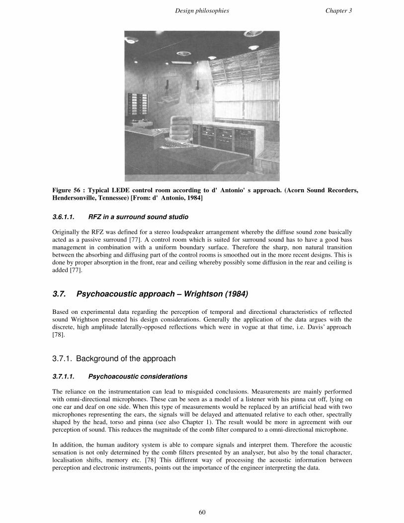
Design philosophies Chapter 3
60
Figure 56 : Typical LEDE control room according to d'Antonio's approach. (Acorn Sound Recorders,Hendersonville, Tennessee) [From: d'Antonio, 1984]
3.6.1.1. RFZ in a surround sound studio
Originally the RFZ was defined for a stereo loudspeaker arrangement whereby the diffuse sound zone basicallyacted as a passive surround [77]. A control room which is suited for surround sound has to have a good bassmanagement in combination with a uniform boundary surface. Therefore the sharp, non natural transitionbetween the absorbing and diffusing part of the control rooms is smoothed out in the more recent designs. This isdone by proper absorption in the front, rear and ceiling whereby possibly some diffusion in the rear and ceiling isadded [77].
3.7. Psychoacoustic approach – Wrightson (1984)
Based on experimental data regarding the perception of temporal and directional characteristics of reflectedsound Wrightson presented his design considerations. Generally the application of the data argues with thediscrete, high amplitude laterally-opposed reflections which were in vogue at that time, i.e. Davis’ approach[78].
3.7.1. Background of the approach
3.7.1.1. Psychoacoustic considerations
The reliance on the instrumentation can lead to misguided conclusions. Measurements are mainly performedwith omni-directional microphones. These can be seen as a model of a listener with his pinna cut off, lying onone ear and deaf on one side. When this type of measurements would be replaced by an artificial head with twomicrophones representing the ears, the signals will be delayed and attenuated relative to each other, spectrallyshaped by the head, torso and pinna (see also Chapter 1). The result would be more in agreement with ourperception of sound. This reduces the magnitude of the comb filter compared to a omni-directional microphone.
In addition, the human auditory system is able to compare signals and interpret them. Therefore the acousticsensation is not only determined by the comb filters presented by an analyser, but also by the tonal character,localisation shifts, memory etc. [78] This different way of processing the acoustic information betweenperception and electronic instruments, points out the importance of the engineer interpreting the data.

Design philosophies Chapter 3
61
3.7.1.2. Application to control room design
3.7.1.2.1. Height of the loudspeakers
The auditory system is very sensitive to the vertical localisation of sound sources, especially in the front. Wrongalignment of the loudspeakers results in auditory confusion. E.g. when the high frequency driver of aloudspeaker is placed below the low frequency driver. With complex sounds containing frequencies above 7kHz, high frequencies are typically localised as ‘higher’ than low frequencies [79]. Therefore placing theloudspeakers upside down can lead to auditory confusion.
3.7.1.2.2. Monitor spacing
In the control rooms there is always at least a stereo set-up of loudspeakers. The distance between theloudspeakers depends on the adequate two-channel mono performance of the sound system and the architectureof the room [78]. When a mono program material is reproduced on the system, we interpret this as an integratedsource. As a result of temporal patterns and instrumental characteristics, misalignment of the loudspeakers canlead to a saxophone be experienced as too wide for instance. Therefore loudspeaker misalignment also results inauditory confusion.
As a solution for this problem Wrightson advocates the use of a centre monitor. This can be used for the monoprogram material. Furthermore as a result of this extra loudspeaker the speaker – loudspeaker – listenerinteraction will be less.
In addition, the height of the loudspeakers with reference to the recording microphone is important. When aloudspeaker has an elevation which is higher than the elevation of the recording microphone, this can also lead toauditory confusion. For instance, when a loudspeaker is located 3 meters above the listener and the signalproduced is recorded at a height of 1.5 meters, the information will be interpreted as that the signal has anelevation of 1.5 meters while it is emanated at say 3 meter above the listener.
3.7.1.2.3. Room reflections
According to the LEDE approach high amplitude, discrete reflections are desired in order to extend the Haaszone. Wrightson states that it was overlooked that the data upon which they based these criteria were generatedwith stimuli which were not appropriate in control rooms. Furthermore he states that the Haas zone aidsinterpretation to the location of the sources in rooms, rather than eliminating audible effects of any reflections[78]. Studies by Wrightson revealed that lateral reflections can be perceived, even when they are as much as 30dB lower in level relative to the direct sound.
Figure 57 : Concept of contra-lateral reflections. [After: Wrightson, 1986]
Another issue Wrightson criticises is the issue of contra lateral reflections because they have consequences inchanging the localisation (see Figure 57). Normally a sound perceived by the ears is spectrally shaped by thepinna, torso, distance etc. This aids to the localisation of the sound signal. According to Wrightson the

Design philosophies Chapter 3
62
introduction of a similar signal with different characteristics, i.e. a contra lateral reflection, will alter theperceived localisation.
3.7.2. Design criteria
As a result of the preceding considerations Wrightson formulated new design criteria. These ought to helpeliminating acoustical aberrations that can provide cues to the perception which may be in variance withinformation provided by the studio audio system. The criteria given by Wrightson are [78]:
1. High amplitude, discrete reflections should be avoided by optimisation of room geometry andfinishes. These reflections create audible degradation of the signal, regardless of the location of thereflecting surface.
2. The integrity of the direct sound field must be maintained. This means reduction in level andnumber of early reflections from monitor shelves, mixing consoles, equipment racks, etc. Thiseffort is enhanced by keeping the vertical and horizontal displacements of the monitor speakers at aminimum to reduce pinna time delay and cross-sensory cues that result in imprecise localisation.
3. Some acoustic energy must be returned to the listening position to ensure user acceptability andpsychological references for existing facilities. This is best accomplished by providing anextremely uncorrelated, homogeneous sound field in both time and frequency domains throughoutthe listening area. This provides a comforting sense of the room for listeners unfamiliar with semi-anechoic conditions. This highly diffuse acoustical energy should exhibit no spectral peaks of morethan 3 dB when measured in 1/3 octave bands and 6 dB for single frequencies, and should be onaverage at least 15 dB lower than the direct signal.
4. Monitor loudspeakers should be located in the vertical plane in a position consistent with typicalmicrophone and instrumental locations.
5. Provisions should be made for single-centre speaker for monitoring of single-channel (true mono)program material.
3.8. Controlled Image Design (CID) – Walker (1993)
In 1993 Walker presented a concept he called Controlled Image Design (CID). Herein the redirection of the earlyreflections in the vicinity of the listener is important to improve image sharpness and make the stereo effect lessroom dependent [81].The key factor in this concept is the use of non absorbing surfaces whereby the designer is not restricted anylonger to a certain amount of absorption in the room. Therefore the reverberation time can be increased whichleads to a more natural environment.
The proposed criterion as a target objective in the CID-method is 20 ms and –20 dB [81]. That is, at a listenerposition no sound energy can be within 20 ms with levels higher than –20 dB relative to the direct sound. Basedon the work carried out in a prototype room, this criterion was later set to 15 ms and –15 dB [80].
3.8.1. Design methodology
Starting with an empty shell and a traditional triangular loudspeaker – listener layout, it is tried to position thereflecting surfaces so that they will not reflect in the direction of the listening position. As a simplification thereare considered only two projections, i.e. plan and elevation. This constrains the reflecting surfaces to be parallelto one of the principal axes of the room [80].
The first step is to specify the listening position and listening area. Although this is geometrically trivial,acoustically there will be some scattering reflections due to diffraction effects. Therefore a zone around thelistening position has to be set where the effects should meet the criterion for all the frequencies. Accordingly acircle is drawn into which no first-order reflections will pass (see Figure 58). In reasonably sized rooms circleswith a diameter of 2.5 to 3.0 meters are feasible [81].

Design philosophies Chapter 3
63
Figure 58 : Plan view with positions of constant tangential reflections. [From: Walker, 1993]
Subsequently a series with the positions of the reflector critical angles has to be found such that any reflection istangential to the circle. As this is a time consuming process he developed a computer program for this purpose.
The curved surfaces as found by the program are not convenient in actual practice. Therefore the curvedpositions are only used as guides to construct planar surfaces. These final flat surface has to be, in a worst casesituation, just tangential to the positions to the circle around the listening positions. The transition occurs insteps. In order to reduce the reverberation time, the transition steps are filled with acoustically absorbingmaterial. Figure 59 presents this implementation.
absorption
Figure 59 : Curved positions are replaced by flat planes. [From: Walker, 1993]
Finally attention has to be paid to the rear wall. The first reflection arriving at the listeners position is comingfrom the rear wall. These reflections have to be attenuated and diffused. When the path distance of the reflectionis approximately 4.5 m longer relative to the direct sound the reflection is already attenuated –10 dB5 [80] [81].Therefore it is not necessary to install large amounts of absorption in the rear wall. Moreover it is not necessaryto use elaborated diffusion such as Schroeder diffusors while alternating acoustic treatment already givesadequate diffusion [81].
5Assuming the distance between the loudspeakers and the listener is approximately 2 meter.

Design philosophies Chapter 3
64
3.8.1.1. Extension for multi-channel control rooms
A few years later the method was extended for multi-channel sound [82]. Herewith it is intended to let a controlroom design meet the criteria given by the ITU and the EBU recommendations. Moreover the CID-method hasbeen simplified.
In a regular shaped control room with six walls and a multi-channel set-up, e.g. with five loudspeakers, there are30 first-order reflections and 150 second-order reflections. As a first simplification the second order reflectionscan be ignored because these have already sufficient time delay and attenuation with the distance [82]. Thereforeonly the first-order reflections of the five loudspeakers which are visible in the listening area are of interest. Bymeans of an image source model the most important reflections can be visualised. Figure 60 (a) shows a few ofthe first order reflections. As it reveals the most potential reflection points are clustered in relatively small areason the walls.
(a) (b)
Figure 60 : First-order wall reflections for half the room (a) and layout of reflecting panels and acoustictreatment, showing control of reflection from Left-Front loudspeaker. [From: Walker, 1998]
Because absorption and diffusion cannot attenuate the reflections enough, the portions of the wall have to beangled in order to redirect the first-order reflections away from the main listening area [82]. This results in atypical layout as presented in Figure 60 (b).
Figure 61 : Control room of the BBC, constructed according to the Controlled Image Design-method.(BBC’s broadcasting House) [From: Walker, 1994]

Design philosophies Chapter 3
65
3.9. Surround Sound approach – WSDG (1999)
Initiated by the film industry surround sound has also become more common in the audio industry. Nevertheless,profound approaches which present a concept or guideline for the design of control rooms suited for multi-channel reproduction are scarcely available at the present.One of the few who have made a set of guidelines for the design of surround sound control rooms is WSDG.They have made an examination of the ITU and EBU recommendations and defined design goals for surroundsound environments. In the next paragraph their practical additions to the ITU and EBU recommendations willbe outlined.
3.9.1. Design goals for a surround sound control room
A properly equipped surround sound control room consists of at least five loudspeakers, i.e. left, centre, right,surround right and surround left, plus a low frequency loudspeaker. In larger rooms any even number ofsurround loudspeakers is acceptable, and provide a larger, more optimum listening area.
In their approach WSDG prefers to flush-mount the loudspeakers. This has a couple of advantages, i.e. reductionof the speaker boundary interference problems, improvement of the low frequent radiation and minimisation ofthe loudspeaker cabinet edge effects [84].If free standing loudspeakers are used, it is important that these are pointed towards the listener. In addition, theuse of anti-vibration mounting equipment is recommended.
Besides the loudspeakers also the reverberation characteristics are considered. In stereophonic control roomsdesigned according to the LEDE approach, it is desired to attain a gap between the direct and reflected sound of15 to 20 ms. In their surround sound approach WSDG advocates that this gap should be the same for all theloudspeakers, i.e. the front loudspeakers as well as the rear loudspeakers. Therefore the LEDE concept is slightlymodified.Extending the original LEDE concept there should be additional absorption behind the surround sound locations,of course only if the loudspeakers are not flush mounted. Furthermore, to prevent uncontrolled reflectionspatterns in time and space heavy absorbing material should be placed on the walls facing the surroundloudspeaker, on-axis of the surround loudspeakers. The application of a diffuse rear wall is still recommended togive the room its natural ambience.

Room acoustical measurements Chapter 4
66
4. Room acoustical measurements
4.1. Introduction
In this chapter the measurements which have been undertaken during the project are presented. Based on theprevious chapters it can be concluded that the design approaches for control rooms differ significantly. Davis’approach by qualifying a control room as a LEDE room only if it confirms to the ETC requirements given byhim (see paragraph 3.5) can be seen as one of the first attempts to qualify a control room objectively.
The measurements have been performed in control rooms which were designed by the known Dutch designersAlex Balster and Ben Kok. Both have been involved in numerous projects in the Netherlands but also abroad. Aseach of them has his own philosophy regarding the design of a control room, the chapter starts with an outline oftheir approaches towards the design of a control room. Subsequently general issues regarding the measurementswill be outlined. The criterion made to use a control room for the project was quite trivial: the control room hadto be designed according to a certain philosophy and has to be qualified as a good control room by the engineerswho work in the rooms.After this general information regarding the measurements, the actual measurements will be discussed. TheIACC and T30 will be related to control rooms. Furthermore the Bonello criterion will be verified by in-situmeasurements.
4.2. Design approaches of the control rooms under test
4.2.1. Suppression of the reflections – Alex Balster
The designs of Alex Balster can generally be seen as a derivative of the design approaches of Michael Rettingerand Tom Hidley6.
According to Balster his designs have to confirm to the following design goals:- Correct choice of the loudspeakers- Symmetrical room- Suppression of discrete reflections- Reverberation time
4.2.1.1. Loudspeakers
According to Balster it is important to start the design process of a control room by primarily determining wherethe room has to be suited for. I.e. has it to be suited for popular music or classical music. This is necessary forthe choice of loudspeakers and for the placement of the loudspeakers.
After deciding the choice of loudspeakers, they are ‘located in the room’ in an equal-sided triangle, with 30 °angles relative to the median plane. In the early days the loudspeakers were slightly inclined, and therefore thetriangle should be a little, i.e. 7,5° inclined. Nowadays, he prefers placing the loudspeakers on level with theears, i.e. at a height of 1.35 m. This should reduce the amount of unwanted reflections by the console.
Another interesting thing to be noted is that according to Balster the engineer position should be inside theloudspeaker – listener triangle. The intention is to create a larger sweet spot.
4.2.1.2. Symmetrical room
For an optimum stereo image it is important that the room is acoustically symmetrical. It is emphasised that theroom should be acoustically symmetrical, because the function of the rooms does not have to be symmetrical.For example, when a window is placed at the left side of the room, the right side of the room has to be
6 Tom Hidley is a known designer of control rooms and studios over the world, e.g. he is the designer of the known DutchWisseloord studios. However his approach is not very scientific and he is more a man of practice. Therefore he did notpresent any papers concerning his philosophy. Generally his approach is comparable to Rettinger’s approach .

Room acoustical measurements Chapter 4
67
acoustically identical. This can be achieved by using a mirror. Another example of acoustical symmetry is theexample of the doors in a room. It is obvious that doors are needed in the control room, but generally one doorfor entering the room is enough. In order to create an acoustical symmetrical room therefore in the opposite wallalso a door should be used. To make this useful the door can be used as e.g. as a closet or as a cloak room.
4.2.1.3. Suppression of reflections
According to Balster, reflections are detrimental to the stereo image, mainly returning reflections from the rearare undesirable. On the other hand some reflections from the front support the localisation, and stereo image.Therefore it is stated by Balster that the sound energy arriving at the engineer’s ears should be 80% direct sound,20 % reflected sound.
To achieve this he constructs sandwich type sidewalls which have to absorb the low and mid frequencies, i.e.100 to 1000 Hz. Further, the rear wall is accommodated with high efficiency broadband absorption, i.e. 10 Hz –20 kHz. If necessary to control room modes or speaker boundary interference problems, the caves behind andnext to the speakers can be used as bass traps.
4.2.1.4. Reverberation time
Generally a reverberation time of say 0.3 seconds is aimed at. It has to be noted that attention has to be paid thatthere will not be a flat reverberation-frequency curve. Actual practice learns the need to compensate for the earcurve and that the musicians ‘miss character’ if the room has a totally flat frequency response.
4.2.2. Reflection control – Ben Kok
Ben Kok has been involved in a lot of studio designs in the Netherlands and Belgium. The design of his studiosand control rooms is strongly determined by the technical and physical aspects of the room and equipment usedin the room, aesthetic considerations are left as much as possible to the project architect and/ or the client.Essentially his ideas of designing a control room can be seen as a side-branch of the LEDE and RFZ concepts.Apart from acoustic considerations, also the logistics are considered essential for a control room (room as aworkspace). According to Kok, the acoustic design of a control should meet the following criteria:
1. Suppression of the early reflections2. Loudspeaker independent design3. Even distribution of the roommodes over frequency and place4. Large sweet spot
In the subsequent subparagraphs these criteria will be outlined in more detail.
4.2.2.1. Suppression of the early reflections
The first reflections are detrimental for the sound image. As a result of these reflections the localisation of thesound image can be ruined but also coloration of the sound image by the early reflections has to be avoided.This is achieved by elaborated application of the RFZ-concept as a further evolution of the LEDE approach of anabsorbing front end of the room and a more live rear end of the room.Most of Ben Kok’s designs do not use Schroeder diffusors. The main reason for this is costs. The application ofthe commercial diffusors is relatively expensive, particularly for relatively small, low cost studios. ThereforeKok incorporates in his designs alternative, custom built diffusing elements, e.g. convex wooden surfaces. Theinside of these elements are often used as ¼λ-traps for low frequencies, something that would not be possiblewith commercial pre-manufactured diffusers..
4.2.2.2. Loudspeaker independent design
One of the main uncertainties a designer has to deal with is the choice of the loudspeaker. When a design isoptimised for a certain pair of loudspeakers, replacement of them with a different type could be ill-fated for thequality of the room. By designing a loudspeaker independent control room, the uncertainty of unexpected effectsdue to replacement of the loudspeakers will be omitted. This guarantees the user as well as the designer a certainquality of the room. According to Kok, this approach is the best way of maintaining specific loudspeaker soundqualities, i.e. what you hear is the loudspeaker, not the room. In addition, the expected life-cycle of the room is
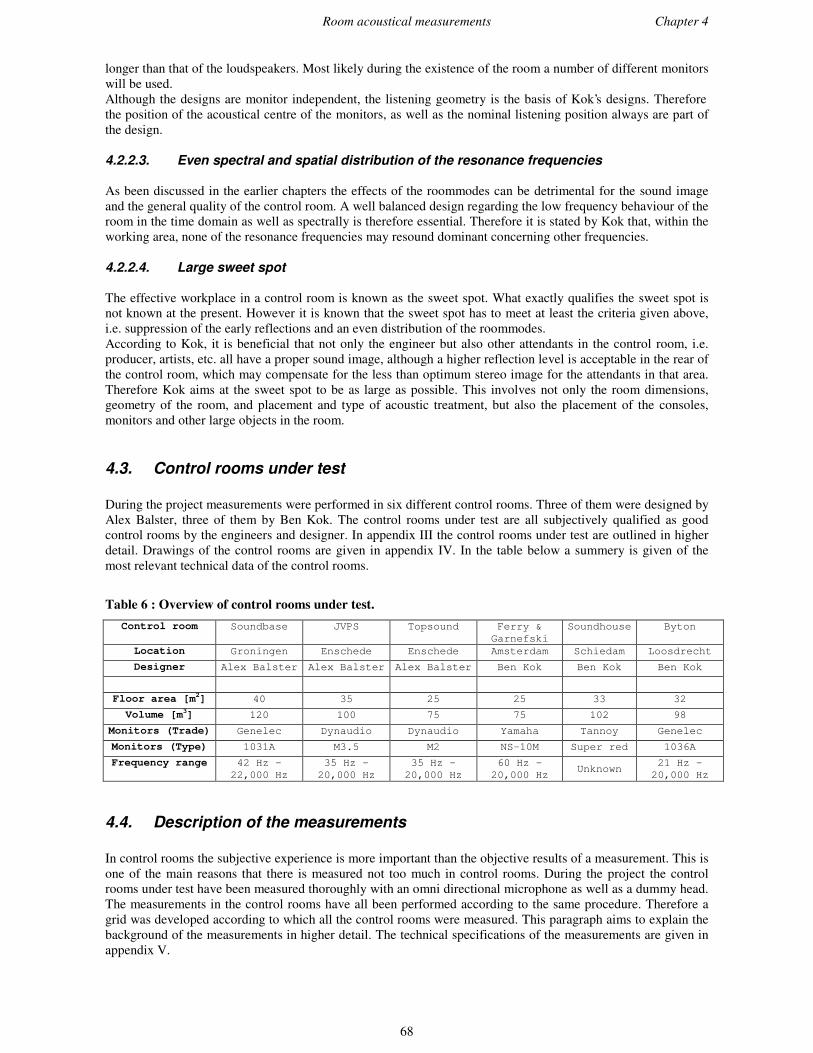
Room acoustical measurements Chapter 4
68
longer than that of the loudspeakers. Most likely during the existence of the room a number of different monitorswill be used.Although the designs are monitor independent, the listening geometry is the basis of Kok’s designs. Thereforethe position of the acoustical centre of the monitors, as well as the nominal listening position always are part ofthe design.
4.2.2.3. Even spectral and spatial distribution of the resonance frequencies
As been discussed in the earlier chapters the effects of the roommodes can be detrimental for the sound imageand the general quality of the control room. A well balanced design regarding the low frequency behaviour of theroom in the time domain as well as spectrally is therefore essential. Therefore it is stated by Kok that, within theworking area, none of the resonance frequencies may resound dominant concerning other frequencies.
4.2.2.4. Large sweet spot
The effective workplace in a control room is known as the sweet spot. What exactly qualifies the sweet spot isnot known at the present. However it is known that the sweet spot has to meet at least the criteria given above,i.e. suppression of the early reflections and an even distribution of the roommodes.According to Kok, it is beneficial that not only the engineer but also other attendants in the control room, i.e.producer, artists, etc. all have a proper sound image, although a higher reflection level is acceptable in the rear ofthe control room, which may compensate for the less than optimum stereo image for the attendants in that area.Therefore Kok aims at the sweet spot to be as large as possible. This involves not only the room dimensions,geometry of the room, and placement and type of acoustic treatment, but also the placement of the consoles,monitors and other large objects in the room.
4.3. Control rooms under test
During the project measurements were performed in six different control rooms. Three of them were designed byAlex Balster, three of them by Ben Kok. The control rooms under test are all subjectively qualified as goodcontrol rooms by the engineers and designer. In appendix III the control rooms under test are outlined in higherdetail. Drawings of the control rooms are given in appendix IV. In the table below a summery is given of themost relevant technical data of the control rooms.
Table 6 : Overview of control rooms under test.Control room Soundbase JVPS Topsound Ferry &
GarnefskiSoundhouse Byton
Location Groningen Enschede Enschede Amsterdam Schiedam Loosdrecht
Designer Alex Balster Alex Balster Alex Balster Ben Kok Ben Kok Ben Kok
Floor area [m2] 40 35 25 25 33 32
Volume [m3] 120 100 75 75 102 98
Monitors (Trade) Genelec Dynaudio Dynaudio Yamaha Tannoy Genelec
Monitors (Type) 1031A M3.5 M2 NS-10M Super red 1036A
Frequency range 42 Hz –22,000 Hz
35 Hz –20,000 Hz
35 Hz –20,000 Hz
60 Hz –20,000 Hz
Unknown21 Hz –20,000 Hz
4.4. Description of the measurements
In control rooms the subjective experience is more important than the objective results of a measurement. This isone of the main reasons that there is measured not too much in control rooms. During the project the controlrooms under test have been measured thoroughly with an omni directional microphone as well as a dummy head.The measurements in the control rooms have all been performed according to the same procedure. Therefore agrid was developed according to which all the control rooms were measured. This paragraph aims to explain thebackground of the measurements in higher detail. The technical specifications of the measurements are given inappendix V.

Room acoustical measurements Chapter 4
69
4.4.1. Measurement positions
The measurement positions are set in a 5x3 matrix with an arbitrarily chosen spacing between the positions of0.5 m. (See Figure 62) The reference position of this matrix is position number eight, which agrees with thedesigned engineer position behind the console. I.e. this position is assumed to be 0.2 m behind the console. Themeasurements are performed on a height of 1.35 m. This is the average height of the ears when a person issitting.
As can be seen in the figure below, the positions 1 to 5 are located above the mixing console. These positions arejustified as these positions can be compared to a person who is actually working, i.e. operating the controls etc.during the mixing process.
CONSOLE
0.5 m
0.5
m
1
76
5432
8
14
10
13
9
1511 12
Figure 62 : Measurement positions; Position eight is the designed engineer position.
It has to be noted that when it was not possible to fully apply the matrix in a room because of e.g. lack of space,the measurement positions have been omitted. So there was not deviated from the matrix. Therefore, as a resultof the furniture in the control room, in the Soundbase control room the positions 1, 6 and 11 have been omitted.Furthermore it has to be noted that during the measurements in the Ferry & Garnefski control room the positions1 and 5 are very close to respectively a loudspeaker and lamp shade. Therefore the measurements with theartificial head had to be omitted at these positions. In addition, due to the equipment racks the measurements atthe positions 10 and 15 are very close to the racks located.
4.4.2. Procedure
All the measurements have been performed according to the 5x3 matrix as outlined in the previous paragraph.The measurement chain used is presented below.
PRE
F:\Bureau\Artik e len\txt fi les IR\Hibox - E nsc hede Right 8 .wav - channel :1 - Pres s ure - Al lpas s H z
[ s]
[ %]
- 100
- 90
- 80
- 70
- 60
- 50
- 40
- 30
- 20
- 10
0
10
20
30
40
50
60
70
80
90
100
0. 0 0 .1 0. 2 0. 3 0. 4 0. 5 0 .6 0. 7 0. 8 0. 9 1. 0 1. 1 1. 2 1 .3
F:\Bureau\Artik e len\txt fi les IR\Hibox - E nsc hede Right 8 .wav - channel :2 - Pres s ure - Al lpas s H z
[ s]
[ %]
- 100
- 90
- 80
- 70
- 60
- 50
- 40
- 30
- 20
- 10
0
10
20
30
40
50
60
70
80
90
100
0. 0 0 .1 0. 2 0. 3 0. 4 0. 5 0 .6 0. 7 0. 8 0. 9 1. 0 1. 1 1. 2 1 .3
Figure 63 : Measurement chain.

Room acoustical measurements Chapter 4
70
As the figure shows the laptop is directly connected to the amplifiers, so the measurement signal is not pre-equalised. Subsequently the amplifiers are directly connected to the loudspeakers. Eventual passive cross overfilters are used as these will not change after tuning the room. The signal used is a non filtered MLS signal with alength of 1.37 s and a sample frequency of 44.1 kHz.During the measurements the in-house loudspeaker system is used. The use of the in-house loudspeakers isjustified because it is assumed that the quality of a control room is an integrated system of the room andloudspeakers which is optimised for the specific room. At every position the room is excited by the left and rightloudspeaker separately.
In every control room the impulse responses of the left en right front loudspeakers are measured separately ateach position with an omni directional microphone and an artificial head. Theoretically this should be the sameresponse because of the acoustical symmetry of the room. The technical data about the equipment used duringthe measurements are given in appendix V.
4.4.2.1. Artificial head
During the artificial head measurements the head is directed straight forward to the screen or window in front ofit. Due to the fact that the end of the microphone standard cannot bend, the artificial head is directed downwardfor the positions 1 to 5 in the matrix. (See Figure 64) Despite the fact that this idea resulted from a practicalshortcoming of the microphone standard, this actually reflects quit well the real work situation of a workingengineer.
Figure 64: Placement of the artificial head
4.5. Binaural measurements
As described in paragraph 1.3.5, the Interaural Cross Correlation (IACC) is a relatively new room acousticparameter, introduced by Ando who evaluated the IACC mainly for large sound fields. Among others the IACCis a good measure for the rate of diffusion in a room. Generally a sound field has to have an IACC of less than0.15 to be subjectively perceived as diffuse [13].There has no literature been found related to the IACC with respect to small sound fields such as they exist incontrol rooms. Therefore the IACC is evaluated for the control rooms under test.
4.5.1. Inter Aural Cross Correlation
4.5.1.1. Goal
Originally the IACC is developed for large rooms such as concert halls and opera houses. In the description ofthe dissimilarity of the signal arrival at the two ears, the ISO 3382 standard splits the time interval in the earlyreflections, t < 80 ms and the late reverberant sound, t > 80 ms. This measurement aims to apply the ISOcriterion to the control rooms under test, which are however small rooms. As a consequence the interpretation ofthe results may need to be adjusted.
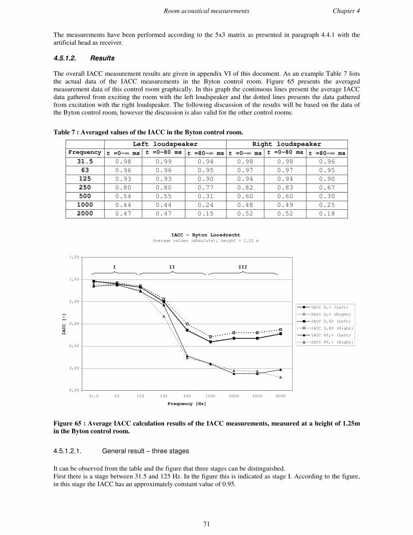
Room acoustical measurements Chapter 4
71
The measurements have been performed according to the 5x3 matrix as presented in paragraph 4.4.1 with theartificial head as receiver.
4.5.1.2. Results
The overall IACC measurement results are given in appendix VI of this document. As an example Table 7 liststhe actual data of the IACC measurements in the Byton control room. Figure 65 presents the averagedmeasurement data of this control room graphically. In this graph the continuous lines present the average IACCdata gathered from exciting the room with the left loudspeaker and the dotted lines presents the data gatheredfrom excitation with the right loudspeaker. The following discussion of the results will be based on the data ofthe Byton control room, however the discussion is also valid for the other control rooms.
Table 7 : Averaged values of the IACC in the Byton control room.
Left loudspeaker Right loudspeakerFrequency t =0-∞∞ ms t =0-80 ms t =80-∞∞ ms t =0-∞∞ ms t =0-80 ms t =80-∞∞ ms
31.5 0.98 0.99 0.94 0.98 0.98 0.9663 0.96 0.96 0.95 0.97 0.97 0.95125 0.93 0.93 0.90 0.94 0.94 0.90250 0.80 0.80 0.77 0.82 0.83 0.67500 0.54 0.55 0.31 0.60 0.60 0.301000 0.44 0.44 0.24 0.48 0.49 0.252000 0.47 0.47 0.15 0.52 0.52 0.18
IACC - Byton Loosdrecht Average values (absolute), height = 1.25 m
0,00
0,20
0,40
0,60
0,80
1,00
1,20
31,5 63 125 250 500 1000 2000 4000 8000
Frequency [Hz]
IACC [-]
IACC 0,+ (Left)
IACC 0,+ (Right)
IACC 0,80 (Left)
IACC 0,80 (Right)
IACC 80,+ (Left)
IACC 80,+ (Right)
I IIIII
Figure 65 : Average IACC calculation results of the IACC measurements, measured at a height of 1.25min the Byton control room.
4.5.1.2.1. General result – three stages
It can be observed from the table and the figure that three stages can be distinguished.First there is a stage between 31.5 and 125 Hz. In the figure this is indicated as stage I. According to the figure,in this stage the IACC has an approximately constant value of 0.95.

Room acoustical measurements Chapter 4
72
Subsequently a second stage can be observed in which the IACC drops. This is indicated in the figure as stage II.Generally this decrease occurs at frequencies between 125 and 2000 Hz. In this control room the IACC dropsfrom 0.95 to 0.44 and 0.49 for respectively the left and right loudspeaker.
Finally there is a third stage in which the IACC seems to be constant again. This occurs for the frequenciesabove 2000 Hz. In case of the Byton control room the IACC is approximately 0.48 and 0.53 for respectively theleft and right loudspeaker.
4.5.1.2.2. Differences between left and right loudspeaker
Besides the information about the IACC during the time, the graphs also reveal that there are differencesbetween the left and right loudspeaker. It can be observed that the average IACC of the left loudspeaker is lowerthan the right loudspeaker in the higher frequency bands. See for example the results of Byton and Soundbase. Apossible explanation for this might be the placement of LCD monitors or other equipment at the left hand side ofthe engineer. Because of these objects early high level reflections will occur when the room is driven by the rightloudspeaker which affects the correlation of the signal perceived between both ears. Consequently the IACC willdecrease.Another reason for the differences between the left and the right loudspeaker might be that both loudspeakers donot have the same radiation pattern due to a difference in the interaction between the wall and the loudspeaker asa result of manually mounting the loudspeaker into the walls.
4.5.1.2.3. Time interval
Figure 65 also reveals important information regarding the chosen time intervals. In the past there has been, andstill there is, a lot of discussion about the proper time intervals. These discussions are mainly related to concerthall acoustics, e.g. [15], [85]. In the room acoustic standard ISO 3382 an interval between 0 and 80 ms has beenchosen which should represent the early reflections, and a time interval from 80 ms to infinity, where infinitycorresponds approximately to the reverberation time. In the figure the results are given for the time intervalsbetween 0 – ∞ ms, 0 – 80 ms and between 80 – ∞ ms for respectively the left and right loudspeaker7.
As the figure shows the difference between the curves showing the IACC of 0 – ∞ ms and of 0 – 80 ms isinsignificant. On the other hand the curve which presents the IACC from 80 – ∞ ms has a totally differentdecline compared to the former ones, although the three stages can also be distinguished in this curve.
According to the graphs it can be concluded that the important information regarding the determination of theIACC in control rooms is given within the 0 – 80 ms time interval. The late energy, thus from 80 – ∞ ms, isinsignificant with respect to the determination of the IACC in this type of rooms.
4.5.1.3. Discussion
4.5.1.3.1. Three stages
As been outlined three stages can be distinguished. It is likely that this can be explained by the interaural timeand intensity differences. As outlined in paragraph 1.3.1.1, due to the shape of our head there are interaural timedifference (ITD) and interaural intensity differences (IID) which affect our ability to localise a soundsource. Theinteraural time differences are the most important cue at the lower end of the frequency range, i.e. at frequenciesbelow 2000 Hz. On the other hand, IID’s are the most important cue above 2000 Hz.
In the first stage the dimensions of the head are very small relative to the wavelength of interest, i.e. thewavelength at 125 Hz is 6.5 times the diameter of an average head. Therefore the phase differences between theears are within half a period. As a result the ears are able to correlate the signals between both ears very well.In the third stage, i.e. above 2000 Hz, the path length differences between the ears is large, whereby it becomesmore difficult for the ears to correlate the signals between the ears. A decrease of the correlation between twosignals implies an increase of perceiving the sound as diffuse, so the IACC will drop.
7 In some graphs in appendix it may seem that not all the curves are drawn, e.g. Soundbase and JVPS. Nevertheless, the linesare all drawn but they are in those cases plotted as one because they fall within the resolution of the graph.

Room acoustical measurements Chapter 4
73
The second stage, i.e. between 250 Hz and 2000 Hz can be seen as a transition zone in which the correlationdecreases relatively quickly with increasing frequency.
It has to be noted that the IACC drops to approximately 0.5. Regarding the control rooms under test this is verylow, however compared to the upper limit given by Ando for subjective experience of diffusion, i.e. IACC<0.15,the room will not be perceived as diffuse.
4.5.1.3.2. Use of the speakers
During the measurements the left and right speaker have been measured separately. The main advantage of thismethod is the possibility to examine the symmetry of the room. This can be done by examining the impulseresponse on a specific position. However, in actual practice the sound is always perceived by at least twoloudspeakers. Additionally, the impulse responses of the left and right loudspeaker at a certain position cannot beadded up. This can introduce large discrepancies, especially in the lower frequencies. Therefore it can be arguedthat there should be measured with both loudspeakers exciting the room together. This would better correlate tothe actual listening circumstances.
4.5.1.3.3. Time interval
To get more insight regarding the IACC during the time, it may be better to choose another time interval, e.g. a50 ms instant. This instant is also used for parameters like the clarity (C50) and Deutlichkeit (D50) whichobjectively qualify the speech characteristics of a room. Generally a room which is well suited for speechtransmission has a relatively short reverberation time, say 0.8 to 1.0 sec (e.g. [85], [86]). As the intervals 0 - ∞ms and 0 – 80 ms hardly differ, it may be interesting for future research to verify the possibilities for theapplication of another time instant, specially for acoustically less reverberant rooms with a non diffuse soundfield.
Furthermore some critics can be given regarding the choice of a time constant itself. There are some argumentsin favour of choosing not a certain time instant, but a certain smoothed time interval. For example instead ofchoosing the interval between 0 and 80 ms, it may be better to choose the interval between 0 and 80 ms wherebyevery interval is smoothed over an interval of say 1 and 5 ms. By smoothing the influence of reflections will bespread in time, especially in this type of rooms where the influence of a reflections is very important this mightbe useful.
4.5.2. Comparison of the different positions within a room
4.5.2.1. Goal
In the previous paragraph the averaged results of the IACC calculations are analysed. The presented data do notgive information regarding the measurement differences in a control room. In order to see to what extent theIACC differs control rooms qualified as good, this paragraph analyses the variation in IACC calculation resultsfor the 1/3-octave bands in the control rooms under test.
4.5.2.2. Results
In appendix VII the results are presented for the left and right loudspeaker separately for all the control roomsunder test. The results presented are based on the time interval between 0 and ∞ ms. The continuous line in thegraphs presents the averaged value of all the calculation results in that specific 1/3-octave band.
The figure and table below present only the results of the Topsound control room, excited by the leftloudspeaker. The discussion will also be based on these data, however it is applicable for all the control roomsunder test.

Room acoustical measurements Chapter 4
74
Topsound - Enschedeleft loudspeaker
0
0,2
0,4
0,6
0,8
1
1,2
10 100 1000 10000
Frequency [Hz]
IACC [-]
Figure 66 : IACC calculation results of the Topsound control room. Time interval used is 0 - ∞∞ ms.
Table 8 : IACC calculation results of the Topsound control room, excited by the left loudspeaker. Timeinterval used is 0 - ∞∞ ms.
Frequency [Hz]LEFTLOUDSPEAKER 31.5 63 125 250 500 1000 2000 4000 8000
Receiver 1 0.98 0.97 0.97 0.94 0.86 0.68 0.72 0.65 0.59Receiver 2 0.98 0.96 0.96 0.94 0.90 0.65 0.63 0.58 0.41Receiver 3 0.97 0.96 0.96 0.82 0.80 0.63 0.59 0.49 0.37Receiver 4 0.95 0.96 0.98 0.89 0.85 0.56 0.48 0.46 0.43Receiver 5 0.94 0.95 0.95 0.83 0.78 0.44 0.32 0.44 0.19Receiver 6 0.99 0.97 0.98 0.95 0.83 0.76 0.74 0.76 0.69Receiver 7 0.99 0.99 0.96 0.91 0.87 0.66 0.60 0.61 0.59Receiver 8 0.99 0.99 0.95 0.79 0.88 0.65 0.45 0.42 0.37Receiver 9 0.98 0.97 0.93 0.80 0.77 0.52 0.43 0.26 0.21Receiver 10 0.99 0.96 0.90 0.56 0.76 0.39 0.42 0.20 0.15Receiver 11 0.99 0.99 0.91 0.94 0.75 0.77 0.68 0.67 0.57Receiver 12 0.99 0.99 0.94 0.87 0.81 0.69 0.61 0.58 0.45Receiver 13 0.99 0.99 0.94 0.79 0.84 0.58 0.57 0.42 0.29Receiver 14 0.99 0.98 0.84 0.84 0.86 0.47 0.50 0.34 0.23Receiver 15 0.99 0.97 0.85 0.72 0.79 0.37 0.50 0.24 0.13
Average 0.98 0.97 0.93 0.84 0.82 0.59 0.55 0.55 0.47
4.5.2.3. Discussion
The results show that at the lower frequencies, i.e. below 250 Hz, the differences between the measured IACCvalues are small. The maximum deviation with the average is 4%. The deviation increases by increasing thefrequency band of interest whereby in the higher end the differences are very large. In the 8000 Hz octave bandthe maximum deviation with the average is 79%.
In contradiction to the general tendency there are two control rooms with deviating results. The first one is theFerry & Garnefski control room. The results of this control room show in the higher frequencies a larger spreadin the measurement results compared to the other control rooms. It is likely that this is due to the asymmetry ofthe room as a consequence of the large equipment racks in the control room. Furthermore in the Byton controlroom it appears that the maximum spread occurs at around 1000 and 2000 Hz instead of the highest frequencies.An explanation for this could not be found.

Room acoustical measurements Chapter 4
75
Based on these results it seems that the dependency of the IACC on the position in the control room increaseswith increasing the frequency band of interest. To confirm this assumption and, moreover, to find out to whatextent this is related to the quality of a control room more extended examination of the small rooms is required.
4.5.3. Influence of the measurement length on the results of the IACC calculation
4.5.3.1. Goal
The length of the measured impulse responses is 1.37 s. According to the ISO 3382 standard the time interval ofinterest for the calculation of the IACC is defined between t1 = 0 and t2 = ∞ ms, where infinity is generally equalto a time of the order of the reverberation time. With respect to a common control room infinity impliesapproximately 0.2 s.
The figure below shows a typical presentation of an impulse response, measured with an artificial head. Thevertical axis presents the relative level in percents, the horizontal axis the measurement length in seconds. Theupper curve presents the right ear, the lower curve the left ear.
F:\Bureau\Artikelen\txt files IR\Hibox - Enschede Right 8.wav - channel:1 - Pressure - Allpass Hz
[s]
[%]
-100
-90
-80
-70
-60
-50
-40
-30
-20
-10
0
10
20
30
40
50
60
70
80
90
100
0.0 0.1 0.2 0.3 0.4 0.5 0.6 0.7 0.8 0.9 1.0 1.1 1.2 1.3
F:\Bureau\Artikelen\txt files IR\Hibox - Enschede Right 8.wav - channel:2 - Pressure - Allpass Hz
[s]
[%]
-100
-90
-80
-70
-60
-50
-40
-30
-20
-10
0
10
20
30
40
50
60
70
80
90
100
0.0 0.1 0.2 0.3 0.4 0.5 0.6 0.7 0.8 0.9 1.0 1.1 1.2 1.3
Figure 67 : Impulse responses of a measurement with an artificial head. The upper curve presents theright ear impulse response, the lower curve the left ear impulse response. The measurement length in thefigure is 1.37 s.
After say 0.15 s the impulse response seems to be flat, however this does not imply that there are no pressurevariations anymore. For instance there will always be some kind of a noise floor due to internal noise of thesystem or background noise. In order to calculate the IACC correctly it has to be prevented that the noise is nottaken into account. To find out to what extent the background noise affects the accuracy of the IACC calculation,the influence of the measurement length on the calculation is examined.

Room acoustical measurements Chapter 4
76
4.5.3.2. Method
To examine the error made in the calculation of the IACC by using an impulse response with a length of 1.37 s.instead of the by ISO 3382 proposed 0.2 s., the impulse responses which are measured at the reference positionwith the left loudspeaker to excitate the room are used and analysed for all the control rooms under test.In order to analyse the influence of the length of the impulse response the end of the impulse responses isstepwise cut off. This results for every control room in impulse responses with a different measurement lengthsof respectively 1.37 s., 1.2 s., 1.0 s., 0.8 s., 0.6 s., 0.4 s., 0.2 s. and 0.1 s. Subsequently the IACC is calculatedfrom the impulse responses.
4.5.3.3. Results and discussion
The results of the analyses are given in appendix VIII. As an example the results of the Ferry & Garnefskicontrol room are presented in the tables below. For the discussion these results will be used, the discussionconcerns all the control rooms under test .
Table 9 : IACC calculation results of the same impulse responses with a different measurement length,calculated over the time interval from 0 - ∞∞ ms.
Frequency [Hz]Time [s]31.5 63 125 250 500 1000 2000 4000 8000
1.37 0.95 0.99 0.99 0.96 0.81 0.84 0.53 0.55 0.321.20 0.95 0.99 0.99 0.96 0.81 0.84 0.53 0.55 0.321.00 0.96 0.99 0.99 0.96 0.81 0.84 0.53 0.55 0.320.80 0.96 0.99 0.99 0.96 0.81 0.84 0.53 0.55 0.320.60 0.97 0.99 0.99 0.96 0.81 0.84 0.53 0.55 0.320.40 0.97 0.99 0.99 0.96 0.81 0.84 0.53 0.55 0.320.20 0.97 0.99 0.99 0.96 0.81 0.84 0.53 0.55 0.320.10 0.97 0.99 0.99 0.96 0.81 0.84 0.53 0.55 0.32
Table 10 : IACC calculation results of the same impulse responses with a different measurement length,calculated over the time interval from 80 - ∞∞ ms.
Frequency [Hz]Time [s]31.5 63 125 250 500 1000 2000 4000 8000
1.37 0.86 0.93 0.94 0.61 0.46 0.32 0.37 0.12 0.061.20 0.85 0.94 0.94 0.62 0.45 0.30 0.37 0.12 0.061.00 0.85 0.94 0.94 0.65 0.43 0.27 0.37 0.13 0.070.80 0.88 0.94 0.94 0.65 0.41 0.26 0.36 0.14 0.070.60 0.91 0.95 0.94 0.65 0.35 0.25 0.36 0.15 0.080.40 0.89 0.95 0.94 0.69 0.26 0.24 0.36 0.15 0.10.20 0.94 0.96 0.95 0.77 0.23 0.24 0.36 0.17 0.110.10 0.99 0.90 0.93 0.83 0.45 0.33 0.41 0.24 0.17
Table 9 shows that the differences in the calculated IACC for the different measurement lengths are insignificantfor the time intervals of 0 – ∞ ms. On the other hand, Table 10 shows relatively large differences for the intervalof 80 – ∞ ms, mainly at the higher frequencies.
The fact that the differences in the late part of the calculation, that is after 80 ms, does not affect the calculationof the IACC for the time interval between 0 and ∞ ms, implies that the energetic contribution of the late part ofthe impulse response is negligible for the IACC calculation. Moreover it can be stated that in control rooms theupper boundary for the time interval to calculate the IACC can be set to 80 ms, due to the fact that the energeticcontribution of the early energy is very large compared to the late energy.
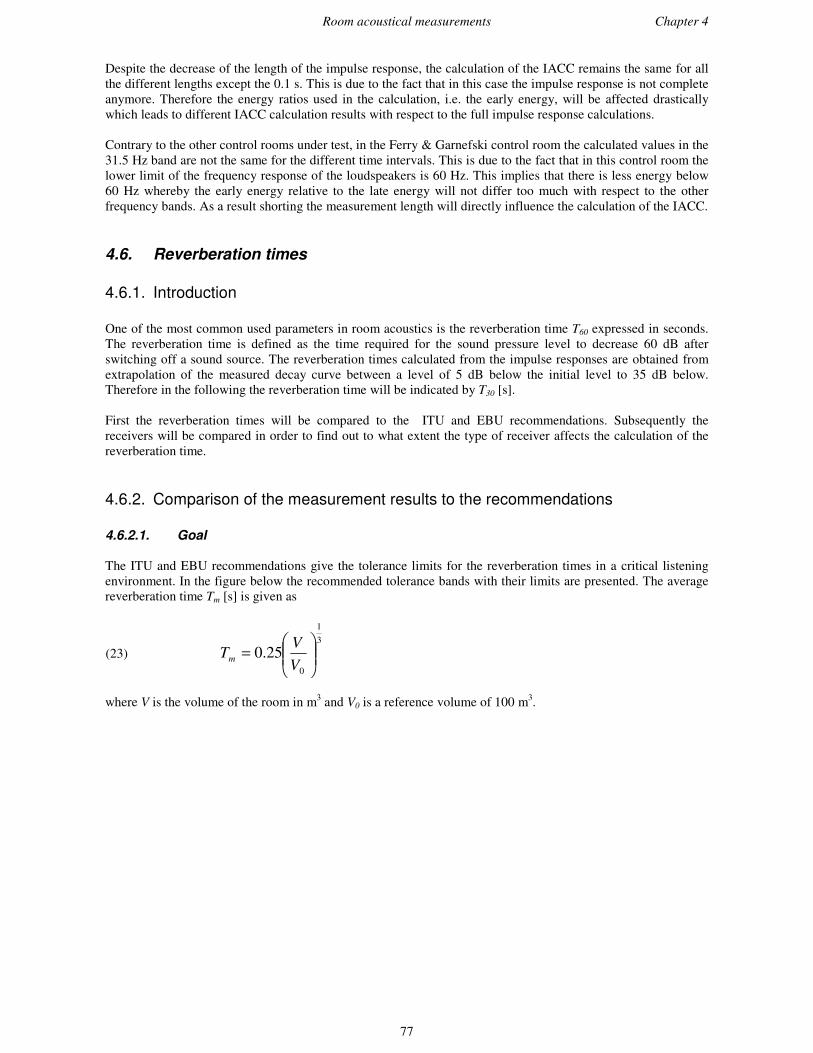
Room acoustical measurements Chapter 4
77
Despite the decrease of the length of the impulse response, the calculation of the IACC remains the same for allthe different lengths except the 0.1 s. This is due to the fact that in this case the impulse response is not completeanymore. Therefore the energy ratios used in the calculation, i.e. the early energy, will be affected drasticallywhich leads to different IACC calculation results with respect to the full impulse response calculations.
Contrary to the other control rooms under test, in the Ferry & Garnefski control room the calculated values in the31.5 Hz band are not the same for the different time intervals. This is due to the fact that in this control room thelower limit of the frequency response of the loudspeakers is 60 Hz. This implies that there is less energy below60 Hz whereby the early energy relative to the late energy will not differ too much with respect to the otherfrequency bands. As a result shorting the measurement length will directly influence the calculation of the IACC.
4.6. Reverberation times
4.6.1. Introduction
One of the most common used parameters in room acoustics is the reverberation time T60 expressed in seconds.The reverberation time is defined as the time required for the sound pressure level to decrease 60 dB afterswitching off a sound source. The reverberation times calculated from the impulse responses are obtained fromextrapolation of the measured decay curve between a level of 5 dB below the initial level to 35 dB below.Therefore in the following the reverberation time will be indicated by T30 [s].
First the reverberation times will be compared to the ITU and EBU recommendations. Subsequently thereceivers will be compared in order to find out to what extent the type of receiver affects the calculation of thereverberation time.
4.6.2. Comparison of the measurement results to the recommendations
4.6.2.1. Goal
The ITU and EBU recommendations give the tolerance limits for the reverberation times in a critical listeningenvironment. In the figure below the recommended tolerance bands with their limits are presented. The averagereverberation time Tm [s] is given as
(23) 31
0
25.0
=
VV
Tm
where V is the volume of the room in m3 and V0 is a reference volume of 100 m3.

Room acoustical measurements Chapter 4
78
1116-01
Tm
Tn
63 100 200 4 000 8 000f (Hz)
+ 0.3 s
+ 0.05 s
– 0.05 s
+ 0.1 s
– 0.1 s
Figure 68 : Tolerance limits for the reverberation time, relative to the average value, Tm [s] [ITU 1116.1,1997]
This examination aims to find out to what extent the measurements are similar to the recommendations in actualpractice. Therefore the reverberation times are calculated for the control rooms under test and plotted togetherwith the tolerance limits given in the recommendations.
4.6.2.2. Results
In the following the results are presented of Jay Vandenberg’s Private Studio (JVPS) control room. The resultsof all the control rooms under test are presented in appendix IX. The discussion of the results will be based onthe JVPS control room, however, generally, it is applicable to all the control rooms.
Because of the different volumes of the control rooms the tolerance limits differ slightly between the differentmeasurements.
Jay Vandenberg's Private Studio - EnschedeLeft loudspeaker
0
0,1
0,2
0,3
0,4
0,5
0,6
10 100 1000 10000
Frequency [Hz]
T30 [s]
ITU limit Min / max Average
Jay Vandenberg's Private Studio - EnschedeRight loudspeaker
0
0,1
0,2
0,3
0,4
0,5
0,6
10 100 1000 10000
Frequency [Hz]
T30 [s]
ITU limit Min / max Average
Figure 69 : Reverberation times T30 [s] of the JVPS control room for the left and right loudspeaker.

Room acoustical measurements Chapter 4
79
Table 11 : Measured reverberation times (T30 [s]) in the JVPS control room.
Left loudspeaker Right loudspeakerFrequency
[Hz]Minimum Maximum Average Minimum Maximum Average
63 0.18 0.47 0.35 0.26 0.47 0.38125 0.19 0.27 0.23 0.15 0.25 0.20250 0.16 0.20 0.19 0.15 0.20 0.19500 0.17 0.22 0.21 0.17 0.23 0.201000 0.20 0.23 0.21 0.18 0.23 0.212000 0.20 0.25 0.21 0.20 0.22 0.214000 0.20 0.22 0.21 0.20 0.21 0.208000 0.18 0.20 0.19 0.17 0.20 0.19
It can be observed that the control rooms under test all agree with the recommendations at the lower frequencies.At frequencies above 125 Hz differences between the control rooms can be recognised. The results of the Bytonand JVPS control rooms comply exactly with the recommendations, although the JVPS control room is close tothe lower limit.
Furthermore it can be seen that the two smallest control rooms under test, i.e. Topsound and Ferry & Garnefski,both have a reverberation time below the lower recommended tolerance limit. Additionally the reverberationtime of the Soundbase control room is at frequencies above 500 Hz also below the lower recommended tolerancelimit. Contradictory to the other control rooms the reverberation time of the Soundhouse control room increasesat higher frequencies.
One of the design issues of a control room is to achieve an environment as neutral as possible. This impliesamong others that it is desired to have a flat frequency response. As can be observed in the figures thereverberation times of JVPS, Topsound, Ferry & Garnefski and Byton all have a flat frequency response in themid and high frequency bands.
4.6.2.3. Discussion
The recommendations given by the ITU and EBU express the tolerance bands in seconds difference relative tothe average reverberation time Tm. It can be argued that this is not expressed on a relative scale. For example, forthe middle frequencies the recommended deviation with respect to Tm is 0.05 s. Regarding the smaller controlrooms this implies that the allowed differences between the average reverberation time and the tolerance bandlimits are relatively large compared to differences in larger control rooms.
Besides the tolerance limits also the fact of measuring the reverberation time in a control room itself can beargued. Essentially the reverberation time is a measure for large rooms with a statistic, homogenous and diffusesound field. As the control rooms are acoustically small environments which are relatively highly absorbingthere is by definition not such a sound field present in this type of rooms.
Moreover a control room is a critical listening environment. As has been outlined in chapter 1 the specularreflections are very important as these can ruin the sound image in a control room. Therefore it might be morerelevant to examine the impulse responses by means of e.g. an ETC plot as these plots comprise a lot ofinformation about the reflections.
As the measurements show, the differences between the minimum and maximum values and the average valuesare approximately identical for all the control rooms, i.e. approximately 0.1 s. difference regarding the averagereverberation time in the mid and high frequency bands. As the control rooms under test are all subjectivelyqualified as good control rooms, it can be stated that the measured reverberation time at different places in agood control room differs between 0.1 seconds irrespective of the volume of the control room. Relatively thisimplies a difference of up to 50%.
The differences between left and right loudspeakers used as the source of excitation are very small. Therefore itcan be stated that in order to calculate the reverberation time of a control room, excitation by only one of theloudspeakers is sufficient to obtain reliable calculations of the reverberation times in a control room.

Room acoustical measurements Chapter 4
80
4.6.3. Comparison of microphones for calculation of the reverberation time
4.6.3.1. Goal
The control rooms under test were all measured with a microphone with omnidirectional receivingcharacteristics, a microphone with so called figure-of-eight receiving characteristics and an artificial head. Inorder to find out to what extent the type of microphone affects the calculation of the reverberation time theresults of one arbitrarily chosen control room are compared.
4.6.3.2. Results
The graphs below present the calculated averaged reverberation times. The graphs show the ITU tolerance limits,and the reverberation times calculated from the impulse responses measured with respectively the omnidirectional microphone, the figure-of-eight microphone and the artificial head microphones. The left and rightartificial head microphones are plotted separately.
0
0,1
0,2
0,3
0,4
0,5
0,6
10 100 1000 10000
Frequency [Hz]
T30 [s]
ITU limits Omni directional Bi directional
Art head | left mic Art head | right mic
0
0,1
0,2
0,3
0,4
0,5
0,6
10 100 1000 10000
Frequency [Hz]
T30 [s]
ITU limits Omni directional Bi directional
Art head | left mic Art head | right mic
Figure 70 : Reverberation times measured with different microphones. The left graph presents the resultsof whereby the room was driven by the left loudspeaker. The right graph presents the reverberation timescalculated from measurements whereby the room was driven by the right loudspeaker.
Table 12 presents the standard deviations σ in seconds between the calculation results for the four differentmicrophones for the left and right loudspeaker separately.
Table 12 : Standard deviations between the reverberation times.
Standard deviation σσ [s]Frequency [Hz] Left loudspeaker Right loudspeaker
63 0.005 0.019125 0.004 0.005250 0.005 0.006500 0.006 0.0061000 0.006 0.0032000 0.005 0.0074000 0.004 0.0048000 0.004 0.005
Average 0.005 0.007
4.6.3.3. Discussion
As the results show the differences between the calculation of reverberation time by using different microphonesare very small, i.e. the average standard deviations for the room excited by respectively the left and rightloudspeaker are 0.005s and 0.007s. As this accuracy is far beyond the common used accuracy regarding the

Room acoustical measurements Chapter 4
81
determination of the reverberation time, it can be stated that all types of used receivers are allowed to apply inorder to measure the reverberation time of a control room.
4.6.4. In situ verification of the Bonello criterion
Discussions concerning the quality of a control room are mainly focussed on the low frequency problems in theroom. In the past there have been a few attempts in order to define the quality of a control room objectively, suchas the LEDE requirements. In this paragraph an attempt is made whereby the Bonello criterion is verified by insitu measurements.
4.6.4.1. Goal
As has been outlined in paragraph 2.3 there is no statistical sound field in the lower frequency bands. Thereforelow frequency anomalies should not be examined statistically but absolute. To examine the low frequencyresponse of a control room in order to qualify the room objectively, the criterion for the distribution ofeigenmodes in a control room as proposed by Bonello in 1981 is used [29]. Essentially this criterion states thatthe energy in the adjacent frequency bands should monotonically increase in order to perceive no coloration.This examination is aimed to verify the criterion in the different control rooms in order to find out if thiscriterion can be a starting point for the objective qualification of a control room.
4.6.4.2. Procedure
In each control room the impulse responses were measured at the different positions on the grid with anomnidirectional microphone. The positions were measured separately for the left and the right loudspeaker.By means of FFT analyses the frequency responses of the impulse responses were generated. Subsequently therms-value of the energy measured in each frequency band was calculated in the 1/3-octave bands between 0 and250 Hz as proposed by Bonello (see Table 13). As the results showed, the measurements contained a certainamount of low frequency energy. This energy is probably a consequence of environmental sound. It iscommonly known that the lower frequencies, say 1 to 15 Hz are the result of air-conditioning systems.Additionally, noise between 15 to say 25 Hz is due to traffic noise. Because the lower limit of most of thespeakers used is between 30 and 40 Hz, it is not likely that the energy below 30 Hz is the result of theloudspeakers and their interaction with the room. Therefore in appendix X the results are plotted from 30 Hz to250 Hz. The frequency band numbers agree with the frequency bands as given in Table 13.
Table 13 : Frequency intervals in Hz used for the calculation of the rms-values.
Band number Frequency band [Hz]0 – 1010 – 1313 – 1616 – 2020 – 25
1 25 – 322 32 – 403 40 – 504 50 – 635 63 – 806 80 – 1007 125 – 1608 160 – 2009 200 – 250
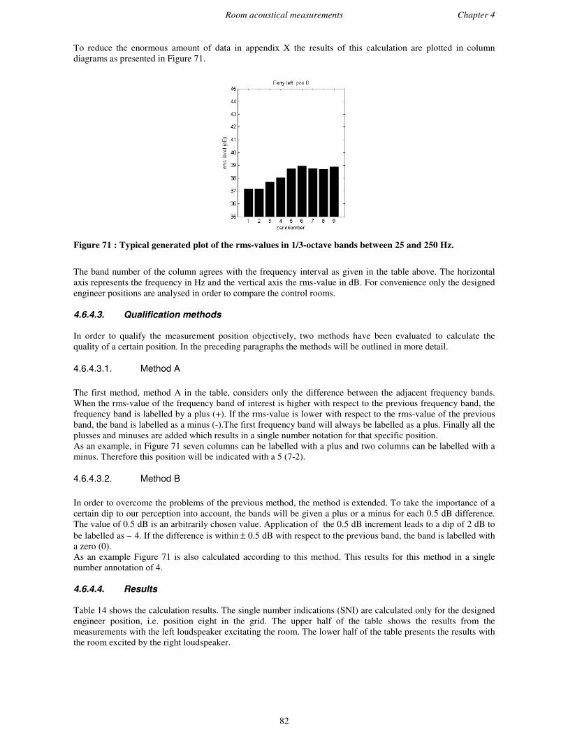
Room acoustical measurements Chapter 4
82
To reduce the enormous amount of data in appendix X the results of this calculation are plotted in columndiagrams as presented in Figure 71.
Figure 71 : Typical generated plot of the rms-values in 1/3-octave bands between 25 and 250 Hz.
The band number of the column agrees with the frequency interval as given in the table above. The horizontalaxis represents the frequency in Hz and the vertical axis the rms-value in dB. For convenience only the designedengineer positions are analysed in order to compare the control rooms.
4.6.4.3. Qualification methods
In order to qualify the measurement position objectively, two methods have been evaluated to calculate thequality of a certain position. In the preceding paragraphs the methods will be outlined in more detail.
4.6.4.3.1. Method A
The first method, method A in the table, considers only the difference between the adjacent frequency bands.When the rms-value of the frequency band of interest is higher with respect to the previous frequency band, thefrequency band is labelled by a plus (+). If the rms-value is lower with respect to the rms-value of the previousband, the band is labelled as a minus (-).The first frequency band will always be labelled as a plus. Finally all theplusses and minuses are added which results in a single number notation for that specific position.As an example, in Figure 71 seven columns can be labelled with a plus and two columns can be labelled with aminus. Therefore this position will be indicated with a 5 (7-2).
4.6.4.3.2. Method B
In order to overcome the problems of the previous method, the method is extended. To take the importance of acertain dip to our perception into account, the bands will be given a plus or a minus for each 0.5 dB difference.The value of 0.5 dB is an arbitrarily chosen value. Application of the 0.5 dB increment leads to a dip of 2 dB tobe labelled as – 4. If the difference is within ± 0.5 dB with respect to the previous band, the band is labelled witha zero (0).As an example Figure 71 is also calculated according to this method. This results for this method in a singlenumber annotation of 4.
4.6.4.4. Results
Table 14 shows the calculation results. The single number indications (SNI) are calculated only for the designedengineer position, i.e. position eight in the grid. The upper half of the table shows the results from themeasurements with the left loudspeaker excitating the room. The lower half of the table presents the results withthe room excited by the right loudspeaker.

Room acoustical measurements Chapter 4
83
Table 14 : Single number indications (SNI) of the designed engineer position.
SNI Method A SNI Method B5 Ferry & Garnefski 4 Ferry & Garnefski3 Topsound 2 JVPS
1 Byton 1 Topsound1 JVPS 0 Byton-1 Soundbase 0 Soundbase
Left
speaker
-3 Soundhouse -2 Soundhouse
5 Ferry & Garnefski 5 Ferry & Garnefski
3 Byton 2 Topsound1 Soundbase 2 Byton-1 JVPS 1 JVPS
-1 Topsound 0 Soundbase
Right
speaker
-3 Soundhouse -4 Soundhouse
4.6.4.5. Discussion
4.6.4.5.1. Method
As the method A only suggests to qualify the adjacent frequency bands with a plus or a minus, the method doesnot consider the spectral position of the dip. For instance a position will be indicated with a 5 when there are e.g.dips in the 40 – 50 Hz and 125 – 160 Hz frequency bands. Another position will also be indicated with a 5,although here the dips are in the 40 – 50 Hz and the 50 – 63 Hz frequency bands.Although both positions are indicated equally, it is likely that the dips in the second example affect ourperception differently compared to the first example.
In addition to the preceding remark, a dip of say 8 dB is more detrimental for our perception than a dip of say 1dB. Although it could possess acoustically critical information, this effect regarding the actual differencesbetween the adjacent frequency bands is also evoked.
The introduced increment of 0.5 dB in method B can lead to wrong conclusions. When the rms-value ofsequential frequency bands is 0.4 dB lower in level, according to the method the result of say 5 bands is 0, whilethe actual dip is 2.0 dB. According to method B all these columns will be labelled as zero, while actually the dipis 2.0 dB which can be detrimental to our perception.
As has been revealed during the explanation of method, the increment of 0.5 dB is arbitrarily chosen. This is avery stringent increment which is assumed to be the least difference in level which can be recognised by alistener.
4.6.4.5.2. Results
The results confirm quite well the shortcomings of method A. It can be visually observed from the graphs inappendix X that the rms-values of the JVPS control room differ less than the Topsound or Byton control room.However, according to method A the SNI of the Byton control room as well as the Topsound control room ishigher than the JVPS control room. As the table shows, method B seems to agree better with the measurements.
The control rooms under test are all subjectively qualified as good control rooms. According to both methods theSNI of the designed engineer position vary over a broad range. It seems that the higher the SNI, the better theagreement with the theoretical criterion as proposed by Bonello. However further research should confirm this.
As can be seen in the graphs of this analysis the differences in rms-values between the adjacent frequency bandsare not as obvious as suggested in the original paper of Bonello. The original article of Bonello considered onlythe distribution of the modes in rectangular room. Moreover there was no weighting regarding the type of mode.Only amount of modes were counted. The control rooms under test were excited by the loudspeakers. Thereforenot only modes are measured, but also other radiated sound energy is measured. Moreover, each measured mode

Room acoustical measurements Chapter 4
84
is naturally ‘weighted’ by the fact if it is a axial, tangential or oblique mode. In accordance with the preceding ithas to be noted that the control rooms under test do all have optimised room dimensions whereby ideally nomodes should be measured.
One of the main goals of a designer is to create an acoustical environment as uniform as possible. The frequencyresponse at a certain position can be satisfactory for our perception. But a control room will be judged as bad ifthere are differences between the frequency responses. Therefore it can be argued that not the frequency responseat a certain position has to be analysed, but difference between two frequency responses at different positions.
The results of the Soundhouse control room are not similar to the other control rooms. The reason herefore isthat during the measurements the signal-to-noise ratio was very poor, mainly in the lower frequency bands.

Conclusions and recommendations Chapter 5
85
5. Conclusions and recommendations
This chapter starts with the overall conclusion that can be drawn from this thesis in general. Hereafter thesubconclusions and recommendations are given. Each chapter is dealt with separately.
5.1. Overall conclusion
The main goal of this project was two folded, on the one hand the aim was to make an inventory of the acousticsof control rooms in general. On the other hand to qualify the control rooms objectively by room acousticalmeasurements.
The acoustics of control rooms consists of an interaction between electroacoustical, psychoacoustical androomacoustical aspects. In order to optimise this interaction it is necessary to fully understand the importance ofeach of the aspects with respect to the design of a control room. Evaluation of the most important designapproaches for stereophonic loudspeaker arrangements revealed that in general these all have similar startingpoints, i.e. time spacing of high level reflections and the low frequency distribution as well as the high frequencydistribution, in order to achieve an optimal acoustical environment.Concerning the surround sound approaches there are no distinct requirements to which a control room shouldmeet at the moment. Generally the present approaches can be seen as an extension of the earlier approaches forstereophonic loudspeaker arrangements.
Regarding the second goal of this thesis, i.e. the objective qualification of a control room, it appeared that despitethe fact that there is nowadays sophisticated measurement equipment available, not too many attempts are madeto qualify control rooms objectively by measurable parameters. As there is no specific standard for the objectivequalification of acoustically small rooms, i.e. control rooms, the applicability of well-known room acousticalparameters for these rooms was evaluated, i.e. IACC and T30. Concerning the IACC it seems that the timeintervals chosen for large room acoustics should be adjusted for small room acoustical purposes. Thereverberation time results showed that despite the absence of a statistical the reverberation time in the controlrooms under test appeared to be quite indifferent to the adjacent measurement positions.Although the methods to verify the Bonello criterion regarding in-situ measurements can be optimised to a largeextent, the proposed approach for the objective qualification of control room can be a starting point for furtherresearch.
5.2. Conclusions
5.2.1. Chapter 1: Human hearing system
5.1. The localisation of a certain sound depends on several factors. The main cues for the localisation in thehorizontal plane are given by the time and intensity differences and by movements of the head. In thevertical plane the pinna reflections are very important in order to determine the elevation of a certain source.As the reflection patterns of the pinna are angle dependent, the pinna acts as a directional filter
5.2. In a stereophonic loudspeaker arrangement with the loudspeakers producing an identical signal whereby thelevel of the loudspeakers are identical and there is no delay between the loudspeakers, a phantom source willoccur in the median plane between the two loudspeakers. By adding a delay between both sources, thephantom source will move towards the undelayed source. As the delay between both sources is between 630µs and 1 ms, the direction of the perceived source is primarily determined by the undelayed source.The time interval hereafter, i.e. between 1 ms and 20 ms, is called the Haas zone. Here the signal of thesignal has to be up to 10 dB higher in level with respect to the direct sound to be perceived separately. Thiszone can be extended by reflections properly spaced in time, known as the Kuttruff effect.
5.3. When the interaural cross correlation IACC is below 0.15, the sound field is perceived as diffuse. This valueis based on room acoustical measurements in large rooms such as concert halls and opera houses. At thismoment no extensive research has been performed which confirms if this value is also valid for small roomsor not.
Conclusions and recommendations Chapter 5
86
5.2.2. Chapter 2: Architectural design issues of a control room
5.4. Regarding the design of control rooms there is no legal frame to which a control room should comply. TheInternational Telecommunication Union (ITU) and the European Broadcasting Union (EBU) have givenrecommendations which a critical listening environment should meet. As these are recommendations andnot a standard, these can be girder for the designer as well as for the client, although they cannot restricteither of them.
5.5. The eigenmodes and other low frequency anomalies are the key issue in order to optimise the geometry of acontrol room. The frequency range of interest concerns the frequencies below the so called Schroederfrequency where the modal density is lower than ten modes per bandwidth.
5.6. In the past there have been lots of attempts to optimise room dimensions. Therefore lots of ratios have beenproposed. In order to give the designer more freedom in his design and to use the volume of a room moreefficient, it is advocated to have a certain area with optimum room dimensions instead of one single ratio.The area of optimum room dimensions proposed by the ITU and EBU seems to be better suited than earlierproposals as the widely spaced modes are weighted more by their introduced quality index.
5.7. The so called Schroeder diffusors are based on mathematical sequences. Besides their diffusing performanceresearch revealed that they also absorb, mainly below the design frequency. Interaction between the wells,poor construction and paint are the main causes for this absorption. By sophisticated use of this knowledge,these absorbing aspects can be integrated in the diffusor without reducing the diffusing quality.
5.8. Although the loudspeaker arrangement of a control room is theoretically recommended by the ITU and EBUto be on a circle, it is sometimes impossible to meet this recommendation. In actual practice it appeared thatincreasing the angle of the loudspeakers with respect to the centre plane shows better results than addingdelays.
5.9. The location of the low frequency loudspeaker or subwoofer should be not on the perpendicular linebetween the walls on which the engineer is located. As a result the loudspeaker will not be able to drive anaxial mode, only tangential or oblique modes. As these are respectively –3 dB and –6 dB lower in levelrelative to an axial mode, these are less detrimental, although still not desirable.
5.2.3. Chapter 3: Design philosophies
5.10. The reflection patterns in time and space relative to our perception of a certain sound image seems to bevery important in the design of a control room. In order to manage this several approaches have beenpresented during the last years. This lead to a shift from acoustically inert rooms to more live rooms whichbetter agree with the actual listening environment of a production, the living room.
5.11. The LEDE concept was the first, and until now only concept, whereby a certain quality of the room hadto be proven by means of an objective measure, i.e. the ETC plot.
5.12. There have been several approaches regarding the design of a control room suited for stereophonicsound reproduction. On the contrary, only few approaches have been presented regarding the design ofcontrol room suited for surround sound reproductions.
5.2.4. Chapter 4: Room acoustical measurements
5.2.4.1. Procedure
5.13. For the measurements in the control rooms under test, the in-house loudspeaker system and amplifierswere used. As these differ for each control room, it is not possible to calibrate the measurement system, i.e.the outgoing part of it, although it can be stated that the in-house loudspeaker system and the amplifiers arean essential part of the whole system whereby the control room is qualified, especially as in most cases this

Conclusions and recommendations Chapter 5
87
loudspeaker system is optimised for the room. Therefore it could be sufficient to only calibrate the receivingpart of the measurement system.
5.2.4.2. Binaural measurements
5.14. The averaged results of the IACC calculations showed that one can generally distinguish three stages.This is explained by the interaural intensity differences and interaural time differences. In the lowerfrequency bands the IACC is between 0.95 and 1.00. In the higher frequency bands the IACC is between0.40 and 0.50. In between there is a transition zone of about two bandwidths where the IACC decreases.According to Ando’s criterion the soundfield is not perceived as diffuse neither in the lower frequencybands nor in the higher frequency bands.
5.15. During the design process of a control room much attention is paid to the symmetry and correctguidance of the reflections in the control room. In actual practice e.g. extra LCD monitors, loudspeakers orother equipment are placed in the control room. Consequently small differences can be observed betweenthe excitation of the room by the left or right loudspeaker. As the criterion to use a control room was that ithad to be objectively qualified as good, it can be stated that small symmetrical distortions are allowed.
5.16. Comparison of the IACC calculation results between the positions revealed that the dependency of theIACC on the measurement position increases by increasing the frequency band of interest. Especially forfrequencies above 125 Hz this is the case.
5.2.4.3. Reverberation measurements
5.17. In the lower frequency bands the control rooms under test all fall within the proposed tolerance bandlimits of the ITU and EBU recommendations. For the mid and higher frequencies the reverberation timeseems to be more volume dependent. As the results show, the smallest control rooms under test havereverberation times below the lower recommended limit, and the rooms with average volume havereverberation times which fall between the recommended limits.
5.18. Comparison to what extent the used microphone during the measurements affects the calculation of thereverberation time revealed that the differences are insignificant. Therefore it can be stated that each type ofmicrophone tested, i.e. omnidirectional, figure-of-eight or artificial head, can be used in order to measureand calculate the reverberation time of the control room.
5.2.4.4. Verification of the Bonello criterion
5.19. A control room is mainly qualified by the low frequency anomalies in the room. Evaluations prior to thedescribed evaluation concerned statistical analyses of the lower frequency bands, i.e. the standard deviationbetween ascending frequency bands was evaluated. Based on this evaluation it appeared that in order to beable to judge the anomalies correctly the absolute values, i.e. rms-values, should be evaluated instead ofusing statistical methods such as the standard deviation.
5.20. It appears that in control rooms which are subjectively qualified as good the differences in the lowerfrequencies of the calculated rms-values fall within ± 2 dB. Contradictory to the original criterion a curvewith a monotonically non decreasing slope cannot be observed clearly. On one hand this is due to the factthat the rooms under test are already optimised rooms. On the other hand, the criterion originally concernsonly the modes in a room, without weighting. During the measurements not only the modes are measured ata certain position, also the redundant energy which cannot be neglected.
5.21. Two methods have been proposed to qualify the characteristic engineer positions in the control roomsunder test with a single number indication (SNI). It appeared that the proposed method B agrees better to thevisual evaluation of the presented graphs.
Conclusions and recommendations Chapter 5
88
5.3. Recommendations
5.3.1. Chapter 2: Architectural design issues of a control room
5.22. The Bonello criterion is based on the so called equal energy concept. As the sound pressure of thedifferent types of modes relative to each other is different, it can be argued to weight the different modes,e.g. by some sort of a smoothing procedure. Additionally the loudness of each band should be used in orderto take the ear sensitivity into account.
5.3.2. Chapter 4: Room acoustical measurements
5.3.2.1. Procedure
5.23. During the measurements with the artificial head only an artificial head without a torso was used. Thiswas mainly due to practical convenience as it was otherwise difficult to measure above the console.However, it is commonly known that the torso also affects the perceived signal. Therefore the absence of atorso can be argued. Further research should examine the influence of the torso on the measurement results.
5.24. During the measurements the right and left loudspeaker were used separately. Because of the symmetryof the control room the frequency responses should be identical. However in actual practise bothloudspeakers will be used. In future examinations whereby the acoustic quality is related to the perception ata certain position, the use of two loudspeakers together seems to be more realistic.
5.25. In order to examine to what extent the acoustical quality of a control room is affected by the in-houseloudspeaker system measurements should be performed with and without the in-house loudspeaker systemin the measurement chain.
5.3.2.1. Binaural measurements
5.26. The length of the impulse response used to calculate the IACC does not affect the calculation results. Itappeared that the calculation results between 0 – 80 ms and 0 – ∞ ms differ insignificantly. On the contrary,the calculation results between 80 - ∞ ms interval differ largely. Therefore it can be stated that thecontribution of the energy after 80 ms is too low in order to contribute to the IACC. In order to be able tomake statements regarding the evolution of the IACC in small rooms during the time, it is proposed to adjustthe time interval. A common known time instant is 50 ms. Future examinations should be performed inorder to see to what extent the proposed time instant for small rooms give more information regarding theevolution of the IACC in time.
5.3.2.2. Reverberation measurements
5.27. The reverberation time is a measure of statistical homogenous environments. In small, heavily dampedenvironments such as control rooms and studios there is per definition no statistical homogenous and diffusesound field present. Therefore the use of the parameter can be argued. It seems to be more relevant toevaluate the actual reflection patterns as these seems to be more important regarding the quality of a certainroom. Further research should confirm this statement.
5.3.2.3. Verification of the Bonello criterion
5.28. Continuous research should be focussed not only on improving the methods but also on consideringmore positions in the control room. Therefore it should be noted that the quality of a control room isdependent on the equality of the control room. This implies that not only the frequency responses at acertain position should be analysed but also the differences between the frequency responses of adjacentmeasurement positions.
5.29. In order to find out to what extend there is any relation to the subjective experience of the control roomand calculated data further research should be performed. Therefore not only control rooms should be usedwhich are subjectively qualified as good but also control rooms which are subjectively qualified as bad. As a

Conclusions and recommendations Chapter 5
89
result statements can also be made regarding the range of results between subjectively as good and badqualified control rooms.

EPILOGUE
90
Epilogue
The epilogue of this document is used to explain the title of this document. During the project there have beenlots of discussions with different kinds of people who are related to control rooms in different ways, amongothers designers, engineers and researchers, about how to define the quality of a control room, advantages anddrawbacks of design methodologies, what materials should be used etc. One of the most remarkable thingsduring the conversations was the importance of the interaction between the engineer and his environment. AsBen Kok remarked very well, a control room is like a shoe: it has to fit the user. To illustrate this, a fewexamples will be given which illustrate perfectly that the quality of a control room is not only acousticallydetermined.
As has been said before a control room and the engineer should be as one. That this is true has beendemonstrated in different ways. For instance, in the control room of Ferry & Garnefski, dance relatedproductions are made. Typical of these productions is the pronounced bass. As they use near field monitors andproduce in a very small control room it is difficult to judge if the low frequency content of the production isenough. Actual practice learned them that when they are standing in one of the corners of the control room, andthe bass sounds there good, they know the low frequency content in their production is good.
Another example to illustrate the interaction of the control room as a whole is illustrated by Ben Kok as well asAlex Balster. In their designs they both advice the customer of a new control room to use the first months afterdelivering up the control room to use the monitors of the old control room. The engineer is so to say calibrated tothe old control room. When he uses his old monitors, he is able to get used, or get calibrated, to the new controlroom. After having been calibrated for the new control room, the new monitors can be used and the engineeragain has to be calibrated.
The relativity of a good acoustical environment is also demonstrated by an example given by Martin Agterbergof the Soundhouse complex. During the design process of the studio complex there is not only paid attention tothe design of the control room, but also to the recording room and the secondary area around the recording andreproduction rooms such as bleu rooms, kitchen, offices etc. One of his productions concerned tango relatedmusic. While searching for the right acoustic ambience for his recording it appeared that not the acousticallywell thought recording room was best suited for the recording of the production but the bleu room.
Besides the relativity of a good acoustic environment, also the visual aspects are very important for the engineerto feel comfortable in the control room. The importance of the visual aspects of a control room is among othersgiven by Bernard Bos of the Topsound studio. About ten years ago he built his own control room. Over the yearshe had made large productions and he as well as his customers seem to be very pleased with their results.However a few years ago Bernard himself did not feel comfortable anymore in his control room. Consequently,according to his personal critics, the results of his productions were less good. Therefore he decided to restylethe control room. This implied not architectural changes but only the taint of the control room was changed, i.e.new colour carpet and a new colour of paint on the walls and ceiling. After this superficial interference, he feltagain comfortable in his control room and the quality of his productions was back on its former level.
A last example of the complexity of control room designs is confirmed by all the engineers. That is, when aproduction is finished on the in-house loudspeaker system, the production is evaluated on another type ofloudspeakers in the control room, and most important on the hi-fi system in the living room or the car audiosystem. If the production is satisfactory on all the systems the production is finished, otherwise there has to betweaked again and again until it is good.
The previous examples illustrate perfectly that a control room which is subjectively qualified as good not onlydepends on the acoustical design but also on several elusive psychological aspects. All these aspects have to bein a certain kind of harmony in order to make the control room qualified as good. Some of the aspects can bephysically explained and optimised, but there are still a lot of things which cannot be easily explained to adopt inthe designs of control rooms. In other words, to fully understand why a control room is qualified as good thereare still a lot of decisions beyond control.

BIBLIOGRAPHY
91
Bibliography
[1] D’Antonio P., Minimizing acoustic distortion in critical listening rooms, presented on a RPG seminar[2] Batteau D.W., Role of the pinna in human localisation, Proc. R. Soc, vol. 168, ser. B, pp. 158 – 180 (1967)[3] http://www.ipo.tue.nl/homepages/dhermes/lectures/SD/ChII.html[4] Bloom P.J., Creating source elevation illusions by spectral manipulation, J. Aud. Eng. Soc, vol 25, pp. 560
– 565, (1977)[5] Puddie Rodgers C.A., Pinna transformations and sound reproduction, J. Aud. Eng. Soc, vol. 29 (4), pp. 226
– 234, (1981, April)[6] De Boer K., Stereofonische geluidsweergave, dissertatie, Delft 1940[7] Blauert J., Spatial hearing – the psychophysics of human sound localisation, revised edition, MIT Press,
1982[8] Haas H., The influence of a single echo on the perceptibility of speech, Acustica, vol 1, pp. 49 – 58 (1951)[9] Wallach H., Newman E.B., Rosenzweig M.R., The precedence effect in sound localization, American J. of
Psychology, vol. LXII, pp. 315 – 316, (1949, July)[10] Davis D., Davis C., Sound system engineering, second edition, Focal Press 1997[11] Alton Everest F., The master handbook of acoustics, 2nd edition, Tab books inc, 1989[12] Gilford C., Acoustics for radio and television studio’s , Peter Peregrinus Ltd 1972[13] Ando Y., Architectural acoustics – blending sound sources, sound fields and listeners, Springer-Verlag New
York, inc., 1998[14] Beranek L.L., Concert and opera halls – how they sound, Acoustical Society of America, American Institute
of Physics, 1996[15] ISO 3382:1997(E), Acoustics – Measurements of the reverberation time of rooms with reference to other
acoustical parameters, Annex B[16] ISO 3382:1997(E), Acoustics – Measurements of the reverberation time of rooms with reference to other
acoustical parameters[17] EBU/UER, Listening conditions for the assessment of sound program material: monophonic and two-
channel stereophonic, Technical document 3276-1997, second edition, http://www.ebu.ch/[18] EBU/UER, Listening conditions for the assessment of sound program material: monophonic and two-
channel stereophonic, Technical document 3276-1999, second edition, http://www.ebu.ch/[19] EBU/UER, Listening conditions for the assessment of sound program material – supplement 1:
multichannel sound, Technical document 3276 http://www.ebu.ch/[20] EBU/UER, Listening conditions for the assessment of sound program material – music, Technical
document 3286-1997, http://www.ebu.ch/[21] EBU/UER, Listening conditions for the assessment of sound program material, Technical Recommendation
R22-1999, http://www.ebu.ch/[22] ITU, Methods for the Subjective Assessment of Small Impairments in Audio Systems including Multichannel
Sound Systems, recommendation ITU-R BS.1116-1 (1997), http://www.itu.in[23] ITU, Multichannel stereophonic sound system with and without accompanying picture, recommendation
ITU-R BS.775-1 (1992-1994),http://www.itu.in[24] AES Technical council, Multichannel surround sound systems and operations, AESTD1001.1.01-10, Audio
Engineering Society, http://www.aes.org[25] Surround Sound Forum, Listening conditions and reproductions arrangements for multichannel
stereophony, Recommended practice SSF01/98, http://www.tonmeister.de/foren/surround/empfehlungen_ssf.htm
[26] Surround Sound Forum, Multichannel recording in 3/2 format, Recommended practice SSF01/98,http://www.tonmeister.de/foren/surround/empfehlungen_ssf.htm
[27] Walker R., Room modes and low frequency responses in small enclosures, AES preprint 4194 (H-7), 100thconvention, 1996, Copenhagen
[28] Kinsler L.E., Frey A.R., Fundamentals of acoustics, second edition, 1952[29] Bonello O.J., A new criterion for the distribution of normal room modes, J. Audio Eng. Soc., vol 29, pp. 597
– 606, 905 (1981 September)[30] Walker R., Low-frequency room responses: Part 2, calculations and measurements, BBC Research and
Development Department Report RD1992/9[31] Schroeder M.R., Die Statistischen Parameter der Frequenzkurven von Grossen Räumen, Acustica Vol. 4,
pp. 594, 1954[32] Schroeder M.R., On frequency response curves in rooms. Comparison of experimental, theoretical, and
Monte Carlo results for the average frequency spacing between maxima, J. Acoust. Soc. Am., 1962, pp. 76– 80

BIBLIOGRAPHY
92
[33] Sabine W.C., Collected papers on acoustics, Peninsula publishing, Los Altos, California USA, 1992[34] Bolt R.H., Note on the normal frequency statistics in rectangular rooms, J. Acoust. Soc. Am., V18(1), pp.
130 – 133, (1946)[35] Sepmeyer L.W., Computed frequency and angular distribution of the normal modes of vibration in
rectangular rooms, J. Acoust. Soc. Am., V37(3), pp. 413 – 423, (1965, March)[36] Louden M.M., Dimension-ratios of rectangular rooms with good distribution of eigentones, Acustica vol.
24, pp 101 – 104, (1971)[37] Bonello O.J., personal contact, May 2002.[38] Walker R., Optimum dimension ratios for small rooms, AES preprint 4192 (H-4), presented at the 100th
convention 1996, Copenhagen[39] EBU/UER, Listening conditions for the assessment of sound program material: monophonic and two-
channel stereophonic, Technical document 3276-1997, second edition, http://www.ebu.ch/[40] ITU, Methods for the Subjective Assessment of Small Impairments in Audio Systems including Multichannel
Sound Systems, recommendation ITU-R BS.1116-1 (1997), http://www.itu.in[41] Cox T.J., d’Antonio P., Determining optimum room dimensions for critical listening environments: a new
methodology, white paper, http://www.rpginc.com/news/library.htm[42] Gilford C.L.S., The acoustic design of talk studios and listening rooms, J. Audio Soc. Am, Vol. 31, pp. 17 –
31, (1979)[43] D’Antonio P., Konnert J.H., The reflection phase grating diffusor: design theory and application, J. Audio
Eng. Soc., vol 32, pp. 228 – 238 (1984 April)[44] D’Antonio P., Konnert J.H., The QRD diffractal: A new one- or two-dimensional fractal sound diffusor, J.
Audio Eng. Soc., vol 40, pp. 117 – 129 (1992 March)[45] Fujiwara K., Miyajima T., Absorption characteristics of a practically constructed Shroeder diffuser of
quadratic-residue type, Applied Acoustics, vol 35, pp. 149 – 152, (1992)[46] Kuttruf H., Sound absorption by pseudostochastic diffusers (Schroeder diffusers), Applied Acoustics, vol
42, pp. 215 – 231, (1994)[47] Fujiwara K., A study on the sound absorption of a quadratic-residue type diffuser, Acustia, vol 81, pp. 370 –
378, (1995)[48] Wu T., Cox T.J., Lam Y.W., A profiled structure with improved low frequency absorption, J. Acoust. Soc.
Am., vol 110, pp. 3064 – 3070 (2001 December)[49] Gilford C., Acoustics for radio and television studios, Peter Peregrinus Ltd., London, England, 1972[50] Mankovsky V.S., Acoustics of studios and auditoria, Focal Press Ltd., London, 1971[51] Cremer L., Müller H.A., Principles and applications of room acoustics – volume 2, Applied Science
publishers, London, 1982[52] Kok B.H.M., Groot E., A mobile for classical recording, Aud. Eng. Soc. Preprint AES convention May
2002 Munich, Germany[53] Mäkivirta A.K., Anet C., A survey study of in-situ stereo and multi-channel monitoring conditions, AES
preprint, 111th AES convention, September 2001, New York, USA.[54] Franssen N.V., Stereofonica, N.V. uitgeversmaatschappij centrex Eindhoven, 1962[55] Noy D., Walters-Storyk Design Group – Europe, personal contact, May 2002[56] Olive S., Schuck P., Sally S., Bonneville M., The effects of loudspeaker placement on listeners’ preference
ratings, J. Aud. Eng. Soc. Vol 42, pp. 651 – 669, (1994, aug)[57] Welti T., How many subwoofers are enough, AES preprint 5602, 112th convention, May 2002, Munich,
Germany[58] Putnam M.T., Recording studio and control room facilities of advance design, J. Audio Eng. Soc, vol 8, pp
111 – 119, (1960, April)[59] Putnam M.T., The loudspeaker and control room as a wholly integrated system, AES preprint 1858 (E-8),
presented at the 70th convention, New York, United States (1980, October)[60] Ballou G., Handbook for sound engineers – the new audio cyclopedia -, Howard W. Sams & company, 1987[61] Veale E.J., The environmental design of a studio control room, AES preprint A-2 (R), presented at the 44th
convention, Rotterdam, the Netherlands (1973, February)[62] Rettinger M., Acoustic considerations in the design of recording studios, 12th annual meeting 1960, AES
preprint 153[63] Rettinger M., On the acoustics of control rooms, AES preprint 1261 (J-1), 57th convention, Los Angeles,
United States (1977)[64] Rettinger M., Studio acoustics, New York: Chemical Publishing Company, Inc., 1981[65] Davis D., The role of the initial time delay gap in the acoustic design of control rooms for recording and
reinforcement systems, AES preprint 1547 (F-3), presented at the 64th convention, New York City, UnitedStates (1979)

BIBLIOGRAPHY
93
[66] Richards R., Nichols G., Translating LEDETM control room design into practical experience, AES preprint1631 G-3), presented at the 66th convention, Los Angeles, United States (1980)
[67] Davis D., Engineering an LEDETM control room for a broadcasting facility, AES preprint 1688 (I-1),presented at the 67th convention, New York, United States (1980)
[68] Davis D., Davis C., The LEDETM concept for the control of acoustic and psychoacoustic parameters inrecording control rooms, J. Aud. Eng. Soc., vol. 29 (9), pp 585 – 595, (1980, September)
[69] Davis C., Meeks G.E., History and development of the LEDE control room concept, AES preprint 1954 (B-5), presented at the 72nd convention, Anaheim, California (1982)
[70] Davis D., Davis C., Tech Topics – Nashville LEDE™ workshop with the oak ridge boys, Syn aud con, vol.12 (1), (1984, fall)
[71] Davis D., Davis C., Tech Topics – Starmusik workshop – Hamburg, Syn aud con, vol. 12 (8), (1985, spring)[72] Davis D., Davis C., Tech Topics – Studio designers workshop, Syn aud con, vol. 15 (1), (1987, fall)[73] Davis D., The LEDE concept, Audio, August 1987[74] Beranek L.L., Music, acoustics and architecture, John Wiley & sons, inc., New York, London, 1962[75] D’Antonio P., Konnert J. H., The RFZ/RPG approach to control room monitoring, AES preprint 2157 (I-6),
presented at the 76th convention, New York, United States (1984)[76] Berger R.E., Tech Topics – Speaker boundary interference response (SBIR), Syn aud con, vol. 11 (5),
(1984)[77] D’Antonio P., personal contact, August 2002[78] Wrightson J. Psychoacoustic considerations in the design of studio control rooms, J. Audio Eng. Soc, vol.
34 (10), pp. 789 – 795, (1986 October)[79] Roffler S.K., Butler R. A., Factors that influence the localisation of sound in the vertical plane, J. Acoust.
Soc. Am., vol 43 (6), pp. 1260 – 1266, (1968)[80] Walker R., A new approach to the design of control room acoustics for stereophony, AES preprint 3543
(G1-1), presented at the 94th convention, Berlin, Germany (1993)[81] Walker R., Early reflections in studio control rooms: the results from the first controlled image design
installations, AES preprint 3853 (P12.6), presented at the 96th convention, Amsterdam, the Netherlands(1994)
[82] Walker R., A controlled-reflections listening room for multi-channel sound, AES preprint 4645 (P8-1),presented at the 98th convention, Amsterdam, the Netherlands (1993)
[83] Walker R., personal contact, July 2002[84] Storyk J., Noy D., Acoustical design criteria for surround sound control rooms, AES preprint 4939 (N4),
presented at the 106th convention, Munich, Germany (1973, May)[85] Keet W de V., The influence of early lateral reflections on spatial impression, 6th International Congress
on Acoustics, Tokyo, 1968[86] Houtgast T., Steeneken H.J.M., Predicting speech intelligibility in rooms from modulation transfer function
– I General room acoustics, Acustica vol. 46 (1980)

94

Beyond Control - Appendices
Acoustics of sound recording control rooms – past, present and future

Beyond Control - Appendices
Acoustics of sound recording control rooms – past, present and future
FAGO report nr: 03.23.G
B.J.P.M. van Munster 447662April 1 2003
Eindhoven University of Technology, the NetherlandsDepartment of ArchitecturePhysical aspects of the built environment group (FAGO)
Graduation committee
Dr. Ir. H.J. Martin (chairman)Prof. Dr. A. Kohlrausch
Ir. C.C.J.M. HakIr. W.C.J.M. Prinssen

TABLE OF CONTENTS
3
Table of contents
TABLE OF CONTENTS ...................................................................................................................................... 3
APPENDIX I: RATIOS ACCORDING TO LOUDEN...................................................................................... 5
APPENDIX II: CALCULATION OF A SCHROEDER DIFFUSOR .............................................................. 6
PRIMITIVE ROOT DIFFUSOR .................................................................................................................................. 6QUADRATIC RESIDUE DIFFUSOR........................................................................................................................... 7REFERENCES ........................................................................................................................................................ 8
APPENDIX III: CONTROL ROOMS UNDER TEST ...................................................................................... 9
INTRODUCTION..................................................................................................................................................... 9CONTROL ROOMS DESIGNED BY ALEX BALSTER .................................................................................................. 9
Soundbase........................................................................................................................................................ 9Jay Vandenberg’s Private Studio (JVPS) ...................................................................................................... 10Topsound ....................................................................................................................................................... 10
CONTROL ROOMS DESIGNED BY BEN KOK ......................................................................................................... 11Ferry & Garnefski ......................................................................................................................................... 11Soundhouse.................................................................................................................................................... 13Byton.............................................................................................................................................................. 13
APPENDIX IV: DRAWINGS OF THE CONTROL ROOMS UNDER TEST ............................................. 15
SOUNDBASE ....................................................................................................................................................... 15JVPS.................................................................................................................................................................. 16TOPSOUND ......................................................................................................................................................... 17FERRY & GARNEFSKI ......................................................................................................................................... 18SOUNDHOUSE ..................................................................................................................................................... 19BYTON ............................................................................................................................................................... 20
APPENDIX V: TECHNICAL SPECIFICATIONS OF THE MEASUREMENTS....................................... 22
APPENDIX VI: AVERAGE VALUES OF THE IACC................................................................................... 23
SOUNDBASE ....................................................................................................................................................... 23JVPS.................................................................................................................................................................. 24TOPSOUND ......................................................................................................................................................... 25FERRY & GARNEFSKI ......................................................................................................................................... 26SOUNDHOUSE ..................................................................................................................................................... 27BYTON ............................................................................................................................................................... 28
APPENDIX VII: 1/3-OCTAVE BAND DISTRIBUTION OF THE IACC .................................................... 29
SOUNDBASE ....................................................................................................................................................... 29JVPS.................................................................................................................................................................. 31TOPSOUND ......................................................................................................................................................... 33FERRY & GARNEFSKI ......................................................................................................................................... 35SOUNDHOUSE ..................................................................................................................................................... 37BYTON ............................................................................................................................................................... 39
APPENDIX VIII: IACC CALCULATED FROM DIFFERENT MEASUREMENT LENGTHS............... 41
SOUNDBASE ....................................................................................................................................................... 41JVPS.................................................................................................................................................................. 42TOPSOUND ......................................................................................................................................................... 43FERRY & GARNEFSKI ......................................................................................................................................... 44SOUNDHOUSE ..................................................................................................................................................... 45BYTON ............................................................................................................................................................... 46

TABLE OF CONTENTS
4
APPENDIX IX: REVERBERATION TIMES IN CONTROL ROOMS ....................................................... 47
SOUNDBASE ....................................................................................................................................................... 47JVPS.................................................................................................................................................................. 48TOPSOUND ......................................................................................................................................................... 49FERRY & GARNEFSKI ......................................................................................................................................... 50SOUNDHOUSE ..................................................................................................................................................... 51BYTON ............................................................................................................................................................... 52
APPENDIX X: LOW FREQUENCY RMS-VALUES AT THE ENGINEER POSITIONS ........................ 53

Ratios according to Louden Appendix I
5
Appendix I: Ratios according to Louden
Below the results of Louden’s examined room dimensions are presented. In order to calculate the standard deviation σ therewas an arbitrarily chosen constant volume of 201.6 m3 used. For all cases Z is considered as 1.
order X Y σσ order X Y σσ order X Y σσ1 1.9 1.4 1.1445 43 1.9 2.8 1.5824 85 1.7 1.8 2.05862 1.9 1.3 1.1542 44 1.6 1.8 1.5896 86 1.3 2.8 2.07353 1.5 2.1 1.1677 45 1.6 2.0 1.5963 87 1.2 2.8 2.07664 1.5 2.2 1.2064 46 1.8 2.6 1.5966 88 1.2 2.7 2.09725 1.2 1.5 1.2158 47 1.1 1.3 1.6011 89 1.5 2.7 2.10036 1.4 2.1 1.2213 48 1.7 1.2 1.6133 90 1.1 2.7 2.10457 1.1 1.4 1.226 49 1.2 1.3 1.6145 91 1.3 2.5 2.11938 1.8 1.4 1.2311 50 1.8 2.8 1.6277 92 1.7 2.8 2.12119 1.6 2.1 1.2488 51 1.6 2.5 1.6289 93 1.5 2.8 2.1341
10 1.2 1.4 1.2612 52 1.4 1.3 1.6479 94 1.7 2.0 2.140911 1.6 1.2 1.2623 53 1.8 2.7 1.6541 95 1.1 2.6 2.155612 1.6 2.3 1.2771 54 1.1 1.2 1.6588 96 1.1 1.9 2.157613 1.6 2.2 1.3178 55 1.2 1.8 1.6692 97 1.2 2.2 2.158514 1.8 1.3 1.3335 56 1.9 1.6 1.6813 98 1.3 2.7 2.168015 1.1 1.5 1.3503 57 1.7 2.1 1.6933 99 1.8 1.9 2.173116 1.6 2.4 1.3841 58 1.3 2.0 1.7038 100 1.6 2.8 2.177217 1.6 1.3 1.4028 59 1.4 2.3 1.7116 101 1.2 2.1 2.194818 1.9 1.5 1.4139 60 1.5 1.6 1.7414 102 1.1 2.4 2.198819 1.1 1.6 1.4285 61 1.7 2.7 1.7693 103 1.2 2.0 2.208020 1.3 1.7 1.4352 62 1.7 2.6 1.7909 104 1.4 2.7 2.236721 1.8 2.3 1.4404 63 1.3 2.2 1.7944 105 1.5 2.6 2.243122 1.9 2.4 1.4527 64 1.9 2.2 1.8097 106 1.8 2.0 2.267023 1.4 2.2 1.4592 65 1.3 1.5 1.8173 107 1.2 2.3 2.284824 1.7 2.3 1.4747 66 1.6 2.6 1.8262 108 1.2 2.4 2.289225 1.7 2.2 1.4839 67 1.1 1.7 1.8352 109 1.1 2.5 2.298626 1.9 2.6 1.4956 68 1.6 1.4 1.8392 110 1.2 1.2 2.322827 1.4 2.0 1.4969 69 1.8 2.1 1.8492 111 1.3 2.6 2.408328 1.3 2.1 1.5038 70 1.5 1.4 1.8668 112 1.6 1.6 2.425929 1.5 2.4 1.5172 71 1.7 1.9 1.8768 113 1.1 2.3 2.429830 1.9 2.3 1.5209 72 1.3 2.4 1.8798 114 1.1 2.1 2.459431 1.9 2.5 1.5233 73 1.4 2.6 1.8949 115 1.1 2.0 2.462232 1.9 2.7 1.5268 74 1.5 2.5 1.9060 116 1.9 2.0 2.501333 1.8 2.5 1.5285 75 1.1 1.8 1.9216 117 1.3 1.3 2.525234 1.5 2.3 1.5291 76 1.4 2.4 1.9286 118 1.5 1.5 2.563935 1.8 2.4 1.5318 77 1.2 2.5 1.9298 119 1.8 1.8 2.645236 1.8 1.5 1.5504 78 1.7 1.6 1.9379 120 1.9 1.9 2.712437 1.7 1.4 1.5598 79 1.4 2.5 1.9665 121 1.7 1.7 2.730038 1.7 2.4 1.5598 80 1.6 2.7 2.0019 122 1.1 2.2 2.745339 1.2 1.9 1.563 81 1.9 2.1 2.0158 123 1.4 1.4 2.816140 1.5 2.0 1.5761 82 1.3 2.3 2.0213 124 1.4 2.8 2.828841 1.7 2.5 1.5785 83 1.2 2.6 2.0260 125 1.7 1.5 1.800442 1.8 2.2 1.5785 84 1.1 2.8 2.0352

Calculation of a Schroeder diffusor Appendix II
6
Appendix II: Calculation of a Schroeder diffusor
Based on the theory presented by Schroeder it is possible to construct diffusing elements. There are two types ofsequences which can be used for constructing one-dimensional and two-dimensional diffusors. The former onesare based on the Primitive Root sequence, the latter ones on the Quadratic Residue sequence.
Primitive Root diffusor
The Primitive Root (PR) diffusor is a one-dimensional diffusor, based on the mathematical PR-sequence givenby
(1) Ng n mod
whereg : least primitive root of Nn : least non negative remainderN : odd prime number
In table 1 the results for a sequence of N = 17 and g = 3 are presented. It canbe observed that this sequence is not mirror symmetrical and only has N-1sequence values.
The bandwidth of the diffusor is defined as the difference between the designfrequency f0 and the maximum frequency fmax of the diffusor. Below f0 andabove fmax the diffraction will not be diffuse but more specular. The designfrequency f0 can be obtained by
(2) NWc
f20 =
whereW : width of the well [m]
d0
W T
Figure 1 : Concept of a Schroeder diffusor
The maximum frequency at which the diffusor is effective, fmax, depends on the width of the well:
(3) Wc
f2max =
The well walls are required to be thin and rigid. In actual models the walls have a finite width T which can betaken in account in the equations (2) and (3) by replacing W by (W + T).
N n2mod 17 3nmod 171 0 -2 1 33 4 94 9 105 16 136 8 57 2 158 15 119 13 1610 13 1411 15 812 2 713 8 414 16 1215 9 216 4 617 1 1
Table 1 : QR- and PR-sequence values for N=17

Calculation of a Schroeder diffusor Appendix II
7
The depth of a well is given by
(4) N
hd Nh 20
mod2 λ
=
wheredh : depth of well h [m]h : well numberλ0 : design wavelength [m]
As the design frequency f0 depends on the total width of the diffuser, the design wavelength λ0 agrees with twicethe width of the diffuser, i.e. 2N(W+T).
The diffraction direction for each wavelength of an incident wave scattered from a one-dimensional diffusor canbe determined by
(5) id NWm αλα sinsin −=
whereαi : angle of incidence [°]αd : angle of diffraction [°]m : positive or negative integer
Using eq. (2), including the wall thickness T, with the assumptions αi = 0°, |sin αd| = 1, an expression for theamount of wells N can be obtained:
(6) )(0 TWf
mcN
+=
The larger the factor m, the greater diffusion will be. Generally for a good diffusion, m can be set as 2, whichyields in five diffraction lobes [1]. Moreover it has to be noticed that N has to be an odd prime number.Generally the calculated value of N has to be adjusted to the next closes larger prime number [1].
Quadratic Residue diffusor
In contradiction to the PR-diffusor, the QR-diffusor satisfies at the design frequency f0 exactly the requirementthat the exponentiated sequence values of the Fourier transform has to have a constant magnitude.The mathematical required QR sequence can be obtained by
(7) Nn mod2
A sequence for N = 17 is also presented in table A1. As it shows the sequence is mirror symmetrical at n = 0 andbetween n = (N + 1)/2. Furthermore it reveals that the sequence is periodic with a period N.
As the QR-diffusor is two dimensional, this also effects the formulae for the depth and the angle of diffraction.To calculate the depth of the well equation (4) has to be extended for the two-dimensional situation, whichresults in
(8) { }N
khd Nkh 2mod22
,λ+=
where h represents the well-number in the one dimensional situation and k the well-number in the twodimensional situation.

Calculation of a Schroeder diffusor Appendix II
8
Finally the diffraction order of a QR-diffusor can be obtained by [2]
(9) ( )
λαα idNWhm
sinsin22 −=+
References
[1] D’Antonio P., Konnert J.H., The reflection phase grating diffusor: design theory and application, J. AudioEng. Soc., vol 32, pp. 228 – 238 (1984 April)
[2] D’Antonio P., Konnert J.H., The QRD diffractal: A new one- or two-dimensional fractal sound diffusor, J.Audio Eng. Soc., vol 40, pp. 117 – 129 (1992 March)

Control rooms under test Appendix III
9
Appendix III: Control rooms under test
Introduction
The control rooms under test are all qualified as very good control rooms by the engineers as well as thedesigners. In this appendix a profound description of the architecture of the control rooms under test is given.Drawings of the control rooms are given in appendix IV.
Control rooms designed by Alex Balster
Soundbase
This control room is one of the most recently completed designs of the control rooms under test, i.e. spring 2002.The Soundbase control room is built in the northern part of the Netherlands in Groningen. The complex consistsof three control rooms and one recording room. As there is a railway close to the complex, one of major issuesduring the design process was the sound insulation of the complex. This is resolved by air cushion springs andproper dilations between the different rooms.
During the measurements the main control room is used. This control room is a high end edit, mix and composeroom for surround 5.1 productions. The control room has a floor area of approximately 40 m2 and a volume ofapproximately 120 m3. The front wall is made of multi layer wooden tiles. In the left and right side of the frontwall the loudspeakers are located. Between the loudspeaker a video screen is positioned. Behind this screen acentre loudspeaker is located.
The side walls are splayed and inclined. These walls are constructed of wood wool cement panels and finishedwith a thin layer of carpet. As can be seen in the drawings, in one of the side walls a door is located which givesentrance to the recording room.
The rear wall is constructed of thick layer of mineral wool in front of a panel resonator. The layer of mineralwool is finished with an acoustic transparent fabric. One corner in the rear wall gives entrance from the corridor.The opposite corner is constructed as a bass trap. In front of the rear wall a sofa is placed. The floor is coveredwith heavy carpet. The ceiling is tilted in the rear and made of wood wool cement elements.
Figure 2 : Soundbase control room - Base 1. Left a front view of the room, including Renger Koning;Right a view of the rear part of the room.
The console is as much as possible integrated in the design. In the middle a large monitor screen is located. Theequipment racks are covered with a thin layer of carpet to avoid disturbing reflections from the rack.
The control room is suited for 5.1 multichannel sound reproduction. During the measurements only the frontmonitors, i.e. Genelec 1031 A, are used. According to the specs these monitors have a frequency response from42 Hz to 22 kHz with a peak level of 120 dB at 1 m by the use of a stereo pair.

Control rooms under test Appendix III
10
It has to be noted that in this control room not all the positions have been measured. At the left of the engineerposition a desk for equipment, synthesiser etc. is located. As it was intended only to measure on the positionsaccording to the grid given in paragraph 4.4.1, it was not possible to measure the positions at the left side, i.e.positions 1, 6 and 11 according to the grid.
Jay Vandenberg’s Private Studio (JVPS)
The second room under test designed by Alex Balster is located in Enschede. The JVPS control room is built in1998 and focussed on the production of CDs of bands. The complex consists of a large control room and a smalliso booth suitable for vocal recording. As this control room is built in a former garage, the main problem duringthe design process of this room was the height. This problem is solved by lowering the floor 0.5 m. As a resultthe room is entered by a small stairway downwards.
The control room has an approximate floor area of 35 m2 and a volume of approximately 100 m3. In the middleof the front wall a large window is located. This window is splayed and inclined to overcome resonanceproblems. The left and right walls are splayed and mounted with monitors, i.e. Dynaudio M3.5. According to thespecs these loudspeakers have a frequency response from 35 to 20 kHz, with a peak level at 1 m distance of 130dB. The walls are mounted with the monitors and are finished with wooden panels. The cavities behind the wallsare filled with mineral wool and act as bass traps.
The side walls are constructed of wood wool cement elements and finished with thin jute layer. The rear side ofthe side walls are parallel to each other. This introduced a disturbing echo between these walls. Therefore on therear wall some furniture and instruments are mounted to give these walls some diffusion. In the wall at the righta door is located to the corridor and a window which gives view to the iso booth.
The rear wall is provided with a panel resonator and a thick layer of mineral wool in front of it, finished with atransparent fabric. The floor is covered with heavy carpet and the ceiling is made of wood wool cementelements.In front of the rear wall the floor is raised about 200 mm. On this floor a sofa is located. Halfway the roomequipment racks are located.
As the pictures show on the console a large amount of loudspeakers and a monitor is placed. During themeasurements these were all removed from the console so the room is measured in a situation which is utmost inagreement with the original design.
Figure 3 : Jay Vandenberg’s control room. Left a front - side view; right a view to the rear of the room.
Topsound
Also located in Enschede is the control room of Topsound. The control room is mainly used for CD productions.The complex exists of a recording room and a reproduction room. The whole complex has approximately the

Control rooms under test Appendix III
11
same floor area as the JVPS studio, however the rooms are differently laid out. Compared to the JVPS controlroom, Topsound has a larger recording room and a smaller reproduction room.
The control room has a floor area of approximately 25 m2 and a volume of 75 m3. The room has a small depth ,i.e. 4.09 m, and a large width, i.e. 6.62 m. As a result the listening position in this room is located close to therear wall.
The front wall of this control room is suited with a window in the middle, which is rotated in the vertical plane aswell as in the horizontal plane to avoid standing waves or unwanted reflections in the room. The 30° splayedwalls are made of painted wooden panels with Dynaudio M2 monitors mounted into the wall. These monitorshave a frequency response from 35 to 20 kHz with a peak level at 1 m distance of 130 dB. The space behind thewalls is filled with mineral wool and act as a bass trap.
The side walls are constructed of wood wool elements and finished with a jute layer. In the right wall a door islocated which connects the room to the corridor. Also in this control room the rear wall is constructed of a panelabsorber with a thick layer of mineral wool in front of it to achieve broadband absorption.
The ceiling is made of wood wool cement elements. In order to avoid standing waves or unwanted reflections atthe engineer position, the ceiling is inclined to the rear. In the rear the ceiling is about 2.6 m high, in the frontabout 2.1 m.The floor is covered with a thick layer of carpet.
Figure 4 : Topsound control room.
Control rooms designed by Ben Kok
Ferry & Garnefski
The control room of Ferry & Garnefski is built in a canal house in the middle of Amsterdam. Due to the fact thatthe canal house is old and small, the main problems during the design process of this control room concernedthe room dimensions and the sound insulation.
The complex consists of a control room which is suited for near field monitoring, a recording room which isabout the same size as the control room and a small voice booth. This voice booth is located in the small spacebetween the recording and reproduction room. During the measurements the Yamaha NS-10M near fieldmonitors are used. These loudspeakers have a frequency range from 60 to 20 kHz.
The room has a floor area of approximately 25 m2 and a volume of approximately 75 m3. As a result of the smallroom dimensions this room is relatively shallow and broad. Therefore the acoustic design differs from regulardesigns by Ben Kok, i.e. the typical LEDE transition are not applied in here.
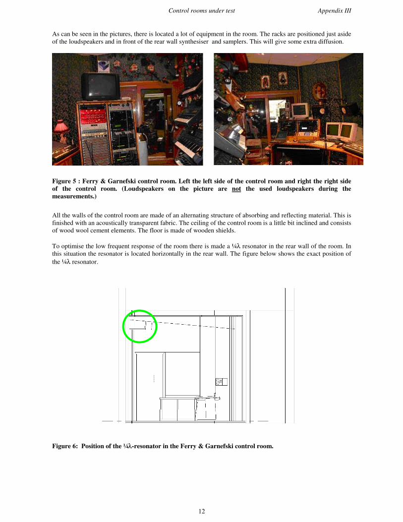
Control rooms under test Appendix III
12
As can be seen in the pictures, there is located a lot of equipment in the room. The racks are positioned just asideof the loudspeakers and in front of the rear wall synthesiser and samplers. This will give some extra diffusion.
Figure 5 : Ferry & Garnefski control room. Left the left side of the control room and right the right sideof the control room. (Loudspeakers on the picture are not the used loudspeakers during themeasurements.)
All the walls of the control room are made of an alternating structure of absorbing and reflecting material. This isfinished with an acoustically transparent fabric. The ceiling of the control room is a little bit inclined and consistsof wood wool cement elements. The floor is made of wooden shields.
To optimise the low frequent response of the room there is made a ¼λ resonator in the rear wall of the room. Inthis situation the resonator is located horizontally in the rear wall. The figure below shows the exact position ofthe ¼λ resonator.
Figure 6: Position of the ¼λλ-resonator in the Ferry & Garnefski control room.

Control rooms under test Appendix III
13
Soundhouse
The Soundhouse control room is built in an old harbour building. The complex exists of three control rooms, tworecording rooms and a large ‘blue room’ where people can have lunch or relax for instance. The control roomunder test has a floor area of approximately 33 m2 and a volume of approximately 103 m3.
The front half of the control room is made of absorbing material, i.e. a thick layer of mineral wool in front of ahardboard panel with high density mineral wool which acts as a panel resonator. As a result the absorption willbe more broadband. Actual practice learned Ben Kok that this construction acts as a baffle, whereby there thelow frequent loading of the loudspeaker will be maintained. In these walls three Tannoy red monitors aremounted.At the right side in the front a large window is suited which gives the engineer a maximum view to the recordingroom. To maintain the acoustical symmetry in the room at the left side a large mirror is located.
The rear half of the room is made of panels in order to reflect the mid and high frequent sound and control thelower frequencies. The rear wall itself is accommodated with diffusors. At the same time these diffusors act as¼λ resonators. Therefore the lower end of the diffusors is closed.In the left side wall a door is suited which gives entrance to the room. At the right, again for acousticalsymmetry, a door is located. This door gives entrance to the machinery room.
The ceiling in the front half of the room is also broad band absorbent. The rear half of the ceiling is constructedas a panel absorber, tuned to absorb the floor-ceiling mode. The floor itself is covered with a linoleum.
As can be seen in the drawings in appendix IV the walls and ceiling have a typical geometry. This is a result ofthe RFZ-method as proposed by d’Antonio. (Paragraph 3.6)
Figure 7 : Soundhouse control room. Left a front view of the control room; Right the rear side of thecontrol room.
Byton
The Byton control room is located in Loosdrecht. The Byton control room has a floor area of approximately 33m2 and a volume of approximately 98 m3. The complex consists of one large control room and a recording room.In addition there is a small near field listening room1.
1 In the original drawings this room is suited as the midi room.

Control rooms under test Appendix III
14
The measurements have been performed in the control room as originally designed by Ben Kok. After themeasurements the mixing console is replaced by a smaller one and the layout of the floor has endured somesmall changes.
Like the Soundhouse control room, the Byton control room has a broadband absorptive front wall. The 30°inclined walls are mounted with Genelec 1036A monitors. These monitors have a frequency response from 21Hz to 20 kHz with a peak level at 1 m distance of 131 dB. In the middle between the loudspeakers a largewindow is mounted which gives view to the recording room.
The rear half of the control room is constructed of a metal stud wall. This provides some extra low frequentabsorption in combination with mid and high frequent reflection. In the left side wall a door is located whichgives entrance to the control room. In order to maintain the acoustical symmetry in the right wall also a door islocated. Herewith the machinery room can be entered. The corners of the rear wall are provided with a diffusingelements which also acts as a ¼λ resonator. Also behind the rear wall a ¼λ resonator is located.
The floor area around the mixing console is covered with linoleum. The rest of the floor area is covered with athin layer of carpet.
The ceiling in the front is made of an effective absorbing construction. The rear half of the ceiling room isconstructed of a resonating panels which are tuned for the floor-ceiling roommode.
Figure 8 : Byton control room. Left a front view of the control room. Right the rear wall of the controlroom.

Drawings of the control rooms under test Appendix IV
15
Appendix IV: Drawings of the control rooms under test
In the figures below the most relevant architectural drawings given. It has to be noted that all the drawings aregiven without any scale factor.
Soundbase
Figure 9 : Plan view of the Soundbase control room.
Figure 10 : Isometric view of the Soundbase studio complex.

Drawings of the control rooms under test Appendix IV
16
JVPS
Figure 11 : Plan view of the JVPS control room.

Drawings of the control rooms under test Appendix IV
17
Topsound
Figure 12 : Plan view of the Topsound control room.

Drawings of the control rooms under test Appendix IV
18
Ferry & Garnefski
Figure 13: Plan view Ferry & Garnefski recording room (left) and control room (right).
Figure 14 : Cross section Ferry & Garnefski control room.

Drawings of the control rooms under test Appendix IV
19
Soundhouse
Figure 15: Plan view Soundhouse control room.
Figure 16: Cross section Soundhouse control room.

Drawings of the control rooms under test Appendix IV
20
Byton
Figure 17 : Plan view Byton control room.
Figure 18 : Cross section Byton control room

Drawings of the control rooms under test Appendix IV
21
Figure 19: Isometric view of the Byton control room.

Technical specifications of the measurements Appendix V
22
Appendix V: Technical specifications of the measurements
Measurement system Dirac V. 2.7 built 1356Laptop Toshiba Tecra 8000Soundcard Yamaha OPL3 SAxMicrophone pre-amp D&R
Omni directional microphone Sennheiser MKH 20Frequency response mic. 12 – 20,000 HzArtificial Head Sennheiser MZK 2002Artificial Head microphones Sennheiser MKE 2002Frequency response AH 40 – 20,000 Hz
Signal MLSFilter None (white noise)Time interval 1.37 sSample rate 48,000 Hz
Post processing Dirac V. 3.0 (Beta) built 1444

Average values of the IACC Appendix VI
23
Appendix VI: Average values of the IACC
The figures and tables below present the averaged measurement results of the IACC, measured at a height of1.25 m. with the artificial head. All the results are presented for the left and right loudspeaker separately. Thetime intervals are chosen according to the ISO 3382 standard.It has to be noted that in some graphs it seems that not all the curves are drawn. e.g. the graph of the Ferry &Garnefski studio. Nevertheless, all the lines are drawn but they are sometimes plotted as one because they fallwithin the resolution of the graph. Therefore also the tables with the actual data is given below each graph.
Soundbase
IACC - Soundbase Groningen Average values (absolute), height = 1.25 m
0,00
0,20
0,40
0,60
0,80
1,00
1,20
31,5 63 125 250 500 1000 2000 4000 8000
Frequency [Hz]
IACC [-]
IACC 0,+ (Left)
IACC 0,+ (Right)
IACC 0,80 (Left)
IACC 0,80 (Right)
IACC 80,+ (Left)
IACC 80,+ (Right)
Left loudspeaker Right loudspeakerFrequency
[Hz]t = 0 - ∞∞ ms t = 0 - 80 ms t = 80 - ∞∞ ms t = 0 - ∞∞ ms t = 0 - 80 ms t = 80 - ∞∞ ms
31.5 0.96 0.97 0.92 0.96 0.97 0.9163 0.98 0.98 0.97 0.98 0.98 0.96
125 0.93 0.93 0.87 0.95 0.96 0.90250 0.68 0.69 0.56 0.76 0.76 0.65500 0.42 0.42 0.28 0.55 0.55 0.28
1000 0.57 0.57 0.26 0.64 0.64 0.262000 0.63 0.63 0.21 0.72 0.72 0.214000 0.63 0.63 0.21 0.72 0.72 0.168000 0.56 0.56 0.15 0.61 0.61 0.10

Average values of the IACC Appendix VI
24
JVPS
IACC - Jay Vandenb erg's Privat e Studio Ensched e
Average values (absolute), height = 1.25 m
0,00
0,20
0,40
0,60
0,80
1,00
1,20
31,5 63 125 250 500 1000 2000 4000 8000
Frequency [Hz]
IACC [-]
IACC 0,+ (Left)
IACC 0,+ (Right)
IACC 0,80 (Left)
IACC 0,80 (Right)
IACC 80,+ (Left)
IACC 80,+ (Right)
Left loudspeaker Right loudspeakerFrequency
[Hz]t = 0 - ∞∞ ms t = 0 - 80 ms t = 80 - ∞∞ ms t = 0 - ∞∞ ms t = 0 - 80 ms t = 80 - ∞∞ ms
31.5 0.99 1.00 0.92 0.97 0.97 0.9063 0.98 0.98 0.94 0.97 0.97 0.94
125 0.96 0.96 0.83 0.95 0.95 0.89250 0.93 0.93 0.59 0.91 0.91 0.56500 0.71 0.71 0.34 0.75 0.75 0.41
1000 0.65 0.65 0.28 0.67 0.67 0.312000 0.59 0.59 0.21 0.61 0.61 0.194000 0.59 0.59 0.21 0.61 0.61 0.168000 0.53 0.54 0.17 0.49 0.49 0.11

Average values of the IACC Appendix VI
25
Topsound
IACC - Topsound EnschedeAverage values (absolute), height = 1.25 m
0,00
0,20
0,40
0,60
0,80
1,00
1,20
31,5 63 125 250 500 1000 2000 4000 8000
Frequency [Hz]
IACC [-]
IACC 0,+ (Left)
IACC 0,+ (Right)
IACC 0,80 (Left)
IACC 0,80 (Right)
IACC 80,+ (Left)
IACC 80,+ (Right)
Left loudspeaker Right loudspeakerFrequency
[Hz]t = 0 - ∞∞ ms t = 0 - 80 ms t = 80 - ∞∞ ms t = 0 - ∞∞ ms t = 0 - 80 ms t = 80 - ∞∞ ms
31.5 0.99 1.00 0.92 0.97 0.97 0.9063 0.98 0.98 0.94 0.97 0.97 0.94
125 0.96 0.96 0.83 0.95 0.95 0.89250 0.93 0.93 0.59 0.91 0.91 0.56500 0.71 0.71 0.34 0.75 0.75 0.41
1000 0.65 0.65 0.28 0.67 0.67 0.312000 0.59 0.59 0.21 0.61 0.61 0.194000 0.59 0.59 0.21 0.61 0.61 0.168000 0.53 0.54 0.17 0.49 0.49 0.11

Average values of the IACC Appendix VI
26
Ferry & Garnefski
IACC - Ferry & Garnefski Amsterdam Average values (absolute), height = 1.25 m
0,00
0,20
0,40
0,60
0,80
1,00
1,20
31,5 63 125 250 500 1000 2000 4000 8000
Frequency [Hz]
IACC [-]
IACC 0,+ (Left)
IACC 0,+ (Right)
IACC 0,80 (Left)
IACC 0,80 (Right)
IACC 80,+ (Left)
IACC 80,+ (Right)
Left loudspeaker Right loudspeakerFrequency
[Hz]t = 0 - ∞∞ ms t = 0 - 80 ms t = 80 - ∞∞ ms t = 0 - ∞∞ ms t = 0 - 80 ms t = 80 - ∞∞ ms
31.5 0.94 0.96 0.87 0.93 0.95 0.9063 0.96 0.96 0.91 0.96 0.96 0.92
125 0.97 0.97 0.93 0.97 0.97 0.93250 0.86 0.87 0.69 0.91 0.91 0.67500 0.72 0.73 0.36 0.76 0.76 0.32
1000 0.59 0.59 0.29 0.57 0.57 0.292000 0.54 0.54 0.22 0.50 0.51 0.214000 0.54 0.54 0.22 0.50 0.51 0.178000 0.51 0.51 0.16 0.52 0.53 0.08

Average values of the IACC Appendix VI
27
Soundhouse
IACC - Soundhouse Schiedam Average values (absolute), height = 1.25 m
0,00
0,20
0,40
0,60
0,80
1,00
1,20
31,5 63 125 250 500 1000 2000 4000 8000
Frequency [Hz]
IACC [-]
IACC 0,+ (Left)
IACC 0,+ (Right)
IACC 0,80 (Left)
IACC 0,80 (Right)
IACC 80,+ (Left)
IACC 80,+ (Right)
Left loudspeaker Right loudspeakerFrequency
[Hz]t = 0 - ∞∞ ms t = 0 - 80 ms t = 80 - ∞∞ ms t = 0 - ∞∞ ms t = 0 - 80 ms t = 80 - ∞∞ ms
31.5 0.99 1.00 0.95 0.98 0.99 0.9363 0.98 0.98 0.97 0.97 0.98 0.95
125 0.95 0.95 0.91 0.94 0.94 0.91250 0.83 0.83 0.63 0.82 0.83 0.61500 0.40 0.42 0.32 0.43 0.44 0.30
1000 0.38 0.40 0.27 0.43 0.45 0.282000 0.45 0.47 0.16 0.44 0.45 0.154000 0.45 0.47 0.16 0.44 0.45 0.178000 0.54 0.55 0.15 0.49 0.50 0.11

Average values of the IACC Appendix VI
28
Byton
IACC - Byton Loosdrecht Average values (absolute), height = 1.25 m
0,00
0,20
0,40
0,60
0,80
1,00
1,20
31,5 63 125 250 500 1000 2000 4000 8000
Frequency [Hz]
IACC [-]
IACC 0,+ (Left)
IACC 0,+ (Right)
IACC 0,80 (Left)
IACC 0,80 (Right)
IACC 80,+ (Left)
IACC 80,+ (Right)
Left loudspeaker Right loudspeakerFrequency
[Hz]t = 0 - ∞∞ ms t = 0 - 80 ms t = 80 - ∞∞ ms t = 0 - ∞∞ ms t = 0 - 80 ms t = 80 - ∞∞ ms
31.5 0.98 0.99 0.94 0.98 0.98 0.9663 0.96 0.96 0.95 0.97 0.97 0.95
125 0.93 0.93 0.90 0.94 0.94 0.90250 0.80 0.80 0.77 0.82 0.83 0.67500 0.54 0.55 0.31 0.60 0.60 0.30
1000 0.44 0.44 0.24 0.48 0.49 0.252000 0.47 0.47 0.15 0.52 0.52 0.18

1/3-octave band distribution of the IACC Appendix VII
29
Appendix VII: 1/3-octave band distribution of the IACC
The figures below present the distribution of the IACC in 1/3-octave bands for control rooms which aresubjectively qualified as good. For each control room the results obtained with the left and right loudspeaker asexcitation source are presented. The IACC in the graphs is calculated for the time interval between 0 and ∞ ms.Besides the separately measured results also the averaged IACC in the specific 1/3-octave band is plotted in thegraphs. The averaged IACC is shown by the continuous curve.
Besides the graphs. for each control room also the actual data for the left and right loudspeaker separately ispresented in the tables.
Soundbase
Soundbase - Groningenleft loudspeaker
0
0,2
0,4
0,6
0,8
1
1,2
10 100 1000 10000
Frequency [Hz]
IACC [-]
Soundbase - Groningenright loudspeaker
0
0,2
0,4
0,6
0,8
1
1,2
10 100 1000 10000
Frequency [Hz]
IACC [-]
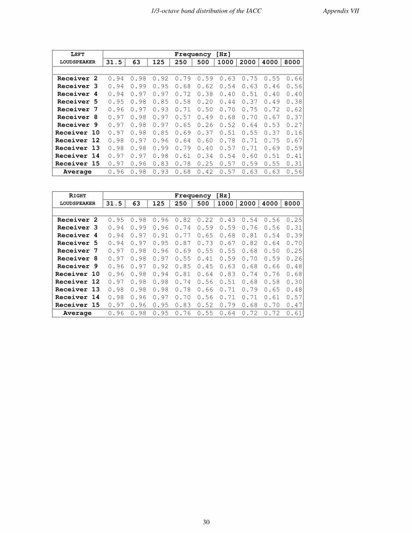
1/3-octave band distribution of the IACC Appendix VII
30
Frequency [Hz]LEFTLOUDSPEAKER 31.5 63 125 250 500 1000 2000 4000 8000
Receiver 2 0.94 0.98 0.92 0.79 0.59 0.63 0.75 0.55 0.66Receiver 3 0.94 0.99 0.95 0.68 0.62 0.54 0.63 0.46 0.56Receiver 4 0.94 0.97 0.97 0.72 0.38 0.40 0.51 0.40 0.40Receiver 5 0.95 0.98 0.85 0.58 0.20 0.44 0.37 0.49 0.38Receiver 7 0.96 0.97 0.93 0.71 0.50 0.70 0.75 0.72 0.62Receiver 8 0.97 0.98 0.97 0.57 0.49 0.68 0.70 0.67 0.37Receiver 9 0.97 0.98 0.97 0.65 0.26 0.52 0.64 0.53 0.27Receiver 10 0.97 0.98 0.85 0.69 0.37 0.51 0.55 0.37 0.16Receiver 12 0.98 0.97 0.96 0.64 0.60 0.78 0.71 0.75 0.67Receiver 13 0.98 0.98 0.99 0.79 0.40 0.57 0.71 0.69 0.59Receiver 14 0.97 0.97 0.98 0.61 0.34 0.54 0.60 0.51 0.41Receiver 15 0.97 0.96 0.83 0.78 0.25 0.57 0.59 0.55 0.31
Average 0.96 0.98 0.93 0.68 0.42 0.57 0.63 0.63 0.56
Frequency [Hz]RIGHTLOUDSPEAKER 31.5 63 125 250 500 1000 2000 4000 8000
Receiver 2 0.95 0.98 0.96 0.82 0.22 0.43 0.54 0.56 0.25Receiver 3 0.94 0.99 0.96 0.74 0.59 0.59 0.76 0.56 0.31Receiver 4 0.94 0.97 0.91 0.77 0.65 0.68 0.81 0.54 0.39Receiver 5 0.94 0.97 0.95 0.87 0.73 0.67 0.82 0.64 0.70Receiver 7 0.97 0.98 0.96 0.69 0.55 0.55 0.68 0.50 0.25Receiver 8 0.97 0.98 0.97 0.55 0.41 0.59 0.70 0.59 0.26Receiver 9 0.96 0.97 0.92 0.85 0.45 0.63 0.68 0.66 0.48Receiver 10 0.96 0.98 0.94 0.81 0.64 0.83 0.74 0.76 0.68Receiver 12 0.97 0.98 0.98 0.74 0.56 0.51 0.68 0.58 0.30Receiver 13 0.98 0.98 0.98 0.78 0.66 0.71 0.79 0.65 0.48Receiver 14 0.98 0.96 0.97 0.70 0.56 0.71 0.71 0.61 0.57Receiver 15 0.97 0.96 0.95 0.83 0.52 0.79 0.68 0.70 0.47
Average 0.96 0.98 0.95 0.76 0.55 0.64 0.72 0.72 0.61

1/3-octave band distribution of the IACC Appendix VII
31
JVPS
Jay Vandenberg's Private Studio - Enschedeleft loudspeaker
0
0,2
0,4
0,6
0,8
1
1,2
10 100 1000 10000
Frequency [Hz]
IACC [-]
Jay Vandenberg's Private Studio - Enschederight loudspeaker
0
0,2
0,4
0,6
0,8
1
1,2
10 100 1000 10000
Frequency [Hz]
IACC [-]

1/3-octave band distribution of the IACC Appendix VII
32
Frequency [Hz]LEFTLOUDSPEAKER 31.5 63 125 250 500 1000 2000 4000 8000
Receiver 1 1.00 0.99 0.98 0.95 0.86 0.84 0.54 0.53 0.58Receiver 2 0.99 0.99 0.98 0.94 0.86 0.74 0.52 0.45 0.45Receiver 3 0.98 0.99 0.96 0.93 0.85 0.63 0.48 0.46 0.34Receiver 4 0.98 0.99 0.93 0.92 0.76 0.68 0.57 0.46 0.27Receiver 5 0.99 0.98 0.94 0.83 0.71 0.65 0.41 0.19 0.18Receiver 6 1.00 0.99 0.98 0.96 0.79 0.79 0.75 0.73 0.36Receiver 7 1.00 0.99 0.98 0.95 0.77 0.75 0.62 0.60 0.31Receiver 8 0.99 0.99 0.95 0.92 0.71 0.68 0.67 0.56 0.23Receiver 9 0.98 0.98 0.94 0.95 0.62 0.58 0.61 0.59 0.20Receiver 10 0.99 0.97 0.96 0.91 0.64 0.48 0.48 0.38 0.13Receiver 11 1.00 0.99 0.96 0.93 0.72 0.76 0.67 0.71 0.33Receiver 12 1.00 0.99 0.95 0.92 0.75 0.61 0.69 0.67 0.24Receiver 13 0.99 0.98 0.97 0.92 0.58 0.58 0.71 0.64 0.28Receiver 14 0.99 0.97 0.96 0.93 0.66 0.52 0.62 0.62 0.20Receiver 15 0.98 0.96 0.98 0.92 0.35 0.49 0.52 0.43 0.16
Average 0.99 0.98 0.96 0.93 0.71 0.65 0.59 0.59 0.53
Frequency [Hz]RIGHTLOUDSPEAKER 31.5 63 125 250 500 1000 2000 4000 8000
Receiver 1 0.99 0.94 0.93 0.81 0.66 0.67 0.43 0.24 0.13Receiver 2 0.96 0.96 0.93 0.87 0.76 0.65 0.56 0.25 0.16Receiver 3 0.93 0.96 0.95 0.90 0.82 0.75 0.54 0.49 0.19Receiver 4 0.96 0.98 0.98 0.94 0.84 0.75 0.50 0.43 0.30Receiver 5 0.99 0.99 0.99 0.95 0.84 0.82 0.71 0.56 0.63Receiver 6 0.98 0.93 0.93 0.89 0.66 0.49 0.47 0.29 0.14Receiver 7 0.95 0.98 0.95 0.90 0.76 0.57 0.59 0.37 0.18Receiver 8 0.94 0.99 0.96 0.89 0.66 0.69 0.70 0.50 0.18Receiver 9 0.98 0.99 0.96 0.92 0.84 0.78 0.58 0.59 0.28Receiver 10 0.99 0.99 0.98 0.96 0.84 0.78 0.78 0.72 0.35Receiver 11 0.97 0.93 0.93 0.92 0.50 0.45 0.49 0.32 0.16Receiver 12 0.95 0.98 0.95 0.94 0.72 0.51 0.62 0.56 0.23Receiver 13 0.96 0.99 0.97 0.94 0.80 0.62 0.63 0.60 0.28Receiver 14 0.98 1.00 0.93 0.94 0.75 0.69 0.75 0.72 0.32Receiver 15 0.99 1.00 0.97 0.95 0.75 0.76 0.77 0.75 0.29
Average 0.97 0.97 0.95 0.91 0.75 0.67 0.61 0.61 0.49

1/3-octave band distribution of the IACC Appendix VII
33
Topsound
Topsound - Enschedeleft loudspeaker
0
0,2
0,4
0,6
0,8
1
1,2
10 100 1000 10000
Frequency [Hz]
IACC [-]
Topsound - Enschederight loudspeaker
0
0,2
0,4
0,6
0,8
1
1,2
10 100 1000 10000
Frequency [Hz]
IACC [-]

1/3-octave band distribution of the IACC Appendix VII
34
Frequency [Hz]LEFTLOUDSPEAKER 31.5 63 125 250 500 1000 2000 4000 8000
Receiver 1 0.98 0.97 0.97 0.94 0.86 0.68 0.72 0.65 0.59Receiver 2 0.98 0.96 0.96 0.94 0.90 0.65 0.63 0.58 0.41Receiver 3 0.97 0.96 0.96 0.82 0.80 0.63 0.59 0.49 0.37Receiver 4 0.95 0.96 0.98 0.89 0.85 0.56 0.48 0.46 0.43Receiver 5 0.94 0.95 0.95 0.83 0.78 0.44 0.32 0.44 0.19Receiver 6 0.99 0.97 0.98 0.95 0.83 0.76 0.74 0.76 0.69Receiver 7 0.99 0.99 0.96 0.91 0.87 0.66 0.60 0.61 0.59Receiver 8 0.99 0.99 0.95 0.79 0.88 0.65 0.45 0.42 0.37Receiver 9 0.98 0.97 0.93 0.80 0.77 0.52 0.43 0.26 0.21Receiver 10 0.99 0.96 0.90 0.56 0.76 0.39 0.42 0.20 0.15Receiver 11 0.99 0.99 0.91 0.94 0.75 0.77 0.68 0.67 0.57Receiver 12 0.99 0.99 0.94 0.87 0.81 0.69 0.61 0.58 0.45Receiver 13 0.99 0.99 0.94 0.79 0.84 0.58 0.57 0.42 0.29Receiver 14 0.99 0.98 0.84 0.84 0.86 0.47 0.50 0.34 0.23Receiver 15 0.99 0.97 0.85 0.72 0.79 0.37 0.50 0.24 0.13
Average 0.98 0.97 0.93 0.84 0.82 0.59 0.55 0.55 0.47
Frequency [Hz]RIGHTLOUDSPEAKER 31.5 63 125 250 500 1000 2000 4000 8000
Receiver 1 0.92 0.96 0.94 0.82 0.78 0.55 0.35 0.44 0.22Receiver 2 0.93 0.95 0.98 0.88 0.90 0.67 0.58 0.57 0.28Receiver 3 0.97 0.95 0.97 0.82 0.85 0.71 0.63 0.56 0.23Receiver 4 0.98 0.96 0.97 0.89 0.86 0.75 0.68 0.58 0.27Receiver 5 0.99 0.97 0.98 0.91 0.83 0.70 0.69 0.60 0.41Receiver 6 0.97 0.95 0.95 0.60 0.68 0.37 0.42 0.24 0.13Receiver 7 0.96 0.98 0.97 0.75 0.77 0.63 0.48 0.44 0.24Receiver 8 0.98 0.99 0.98 0.85 0.84 0.65 0.58 0.54 0.47Receiver 9 0.99 0.99 0.97 0.86 0.79 0.78 0.73 0.73 0.62Receiver 10 0.99 0.98 0.96 0.89 0.76 0.74 0.79 0.78 0.63Receiver 11 0.98 0.96 0.91 0.66 0.73 0.60 0.44 0.39 0.22Receiver 12 0.98 0.97 0.93 0.77 0.85 0.54 0.51 0.53 0.30Receiver 13 0.99 0.99 0.98 0.83 0.82 0.69 0.61 0.56 0.43Receiver 14 0.99 0.99 0.94 0.90 0.84 0.82 0.79 0.72 0.55Receiver 15 0.99 0.99 0.89 0.92 0.68 0.76 0.74 0.78 0.61
Average 0.97 0.97 0.95 0.82 0.80 0.66 0.60 0.60 0.56

1/3-octave band distribution of the IACC Appendix VII
35
Ferry & Garnefski
Ferry & Garnefski - Amsterdamleft loudspeaker
0
0,2
0,4
0,6
0,8
1
1,2
10 100 1000 10000
Frequency [Hz]
IACC [-]
Ferry & Garnefski - Amsterdamright loudspeaker
0
0,2
0,4
0,6
0,8
1
1,2
10 100 1000 10000
Frequency [Hz]
IACC [-]

1/3-octave band distribution of the IACC Appendix VII
36
Frequency [Hz]LEFTLOUDSPEAKER 31.5 63 125 250 500 1000 2000 4000 8000
Receiver 2 0.98 0.99 0.99 0.97 0.91 0.85 0.79 0.60 0.38Receiver 3 0.96 0.98 0.96 0.91 0.80 0.69 0.55 0.36 0.28Receiver 4 0.97 0.97 0.99 0.74 0.65 0.42 0.48 0.38 0.23Receiver 5 0.98 0.95 0.97 0.50 0.61 0.38 0.36 0.31 0.22Receiver 6 0.89 0.99 0.97 0.89 0.76 0.73 0.54 0.61 0.60Receiver 7 0.92 0.99 0.98 0.97 0.83 0.88 0.84 0.80 0.79Receiver 8 0.95 0.99 0.99 0.96 0.81 0.84 0.53 0.55 0.32Receiver 9 0.92 0.97 0.96 0.92 0.74 0.23 0.52 0.38 0.13Receiver 10 0.95 0.95 0.96 0.76 0.69 0.35 0.35 0.46 0.12Receiver 11 0.84 0.98 0.95 0.92 0.67 0.61 0.47 0.65 0.58Receiver 12 0.92 0.98 0.99 0.94 0.82 0.84 0.83 0.74 0.68Receiver 13 0.95 0.97 0.98 0.96 0.79 0.75 0.53 0.51 0.32Receiver 14 0.92 0.94 0.94 0.89 0.55 0.54 0.49 0.46 0.14Receiver 15 0.97 0.80 0.96 0.76 0.51 0.18 0.29 0.33 0.11
Average 0.94 0.96 0.97 0.86 0.72 0.59 0.54 0.54 0.51
Frequency [Hz]RIGHTLOUDSPEAKER 31.5 63 125 250 500 1000 2000 4000 8000
Receiver 2 0.94 0.91 0.98 0.83 0.71 0.24 0.39 0.35 0.07Receiver 3 0.95 0.97 0.99 0.92 0.83 0.51 0.62 0.35 0.21Receiver 4 0.96 0.99 0.99 0.98 0.82 0.82 0.70 0.51 0.23Receiver 5 0.97 0.98 0.97 0.96 0.76 0.78 0.41 0.66 0.71Receiver 6 0.90 0.94 0.94 0.74 0.60 0.36 0.38 0.31 0.11Receiver 7 0.81 0.92 0.96 0.84 0.75 0.57 0.36 0.35 0.13Receiver 8 0.92 0.98 0.98 0.94 0.85 0.43 0.47 0.57 0.15Receiver 9 0.95 0.99 0.99 0.97 0.78 0.71 0.64 0.51 0.36Receiver 10 0.98 0.99 0.99 0.99 0.87 0.88 0.54 0.74 0.56Receiver 11 0.94 0.95 0.90 0.80 0.65 0.15 0.18 0.44 0.13Receiver 12 0.84 0.84 0.96 0.91 0.68 0.24 0.40 0.58 0.20Receiver 13 0.91 0.96 0.97 0.91 0.80 0.49 0.50 0.42 0.34Receiver 14 0.98 0.99 0.99 0.94 0.76 0.89 0.83 0.75 0.51Receiver 15 0.99 0.98 0.99 0.96 0.79 0.87 0.64 0.80 0.50
Average 0.93 0.96 0.97 0.91 0.76 0.57 0.50 0.50 0.52

1/3-octave band distribution of the IACC Appendix VII
37
Soundhouse
Soundhouse - Schiedamleft loudspeaker
0
0,2
0,4
0,6
0,8
1
1,2
10 100 1000 10000
Frequency [Hz]
IACC [-]
Soundhouse - Schiedamright loudspeaker
0
0,2
0,4
0,6
0,8
1
1,2
10 100 1000 10000
Frequency [Hz]
IACC [-]

1/3-octave band distribution of the IACC Appendix VII
38
Frequency [Hz]LEFTLOUDSPEAKER 31.5 63 125 250 500 1000 2000 4000 8000
Receiver 1 0.99 0.98 0.98 0.94 0.41 0.45 0.62 0.66 0.59Receiver 2 0.99 0.98 0.96 0.92 0.56 0.51 0.51 0.59 0.63Receiver 3 0.99 0.99 0.93 0.81 0.59 0.47 0.45 0.39 0.44Receiver 4 0.99 0.99 0.91 0.80 0.58 0.44 0.34 0.36 0.35Receiver 5 0.99 0.97 0.92 0.80 0.30 0.22 0.27 0.28 0.20Receiver 6 0.99 0.99 0.97 0.91 0.24 0.50 0.58 0.73 0.49Receiver 7 0.99 0.98 0.96 0.90 0.45 0.43 0.61 0.75 0.56Receiver 8 0.99 0.98 0.94 0.82 0.36 0.41 0.56 0.65 0.40Receiver 9 0.98 0.98 0.94 0.81 0.43 0.35 0.36 0.47 0.26Receiver 10 0.99 0.97 0.90 0.79 0.50 0.26 0.31 0.42 0.25Receiver 11 0.99 1.00 0.96 0.82 0.21 0.39 0.53 0.60 0.50Receiver 12 0.99 0.99 0.96 0.87 0.35 0.39 0.52 0.69 0.45Receiver 13 0.98 0.97 0.95 0.76 0.39 0.32 0.47 0.60 0.42Receiver 14 0.97 0.96 0.98 0.78 0.31 0.35 0.32 0.42 0.17Receiver 15 0.99 0.97 0.95 0.68 0.35 0.20 0.36 0.45 0.19
Average 0.99 0.98 0.95 0.83 0.40 0.38 0.45 0.45 0.54
Frequency [Hz]RIGHTLOUDSPEAKER 31.5 63 125 250 500 1000 2000 4000 8000
Receiver 1 0.98 0.95 0.90 0.67 0.54 0.32 0.31 0.34 0.14Receiver 2 0.97 0.97 0.87 0.82 0.49 0.47 0.39 0.33 0.21Receiver 3 0.97 0.98 0.93 0.82 0.51 0.47 0.42 0.47 0.44Receiver 4 0.98 0.99 0.97 0.89 0.51 0.63 0.53 0.72 0.62Receiver 5 0.98 0.99 0.98 0.93 0.35 0.58 0.58 0.58 0.67Receiver 6 0.98 0.95 0.93 0.70 0.46 0.27 0.31 0.33 0.20Receiver 7 0.97 0.96 0.90 0.79 0.50 0.35 0.32 0.33 0.20Receiver 8 0.98 0.98 0.92 0.86 0.49 0.44 0.48 0.57 0.40Receiver 9 0.98 0.98 0.97 0.91 0.30 0.59 0.51 0.59 0.47Receiver 10 0.99 0.99 0.98 0.91 0.41 0.49 0.66 0.67 0.45Receiver 11 0.96 0.95 0.95 0.74 0.33 0.31 0.21 0.28 0.15Receiver 12 0.95 0.97 0.96 0.82 0.46 0.39 0.36 0.34 0.25Receiver 13 0.97 0.98 0.96 0.78 0.49 0.36 0.44 0.60 0.42Receiver 14 0.99 0.99 0.97 0.85 0.22 0.34 0.49 0.59 0.45Receiver 15 0.99 0.99 0.96 0.82 0.43 0.42 0.54 0.55 0.38
Average 0.98 0.97 0.94 0.82 0.43 0.43 0.44 0.44 0.49
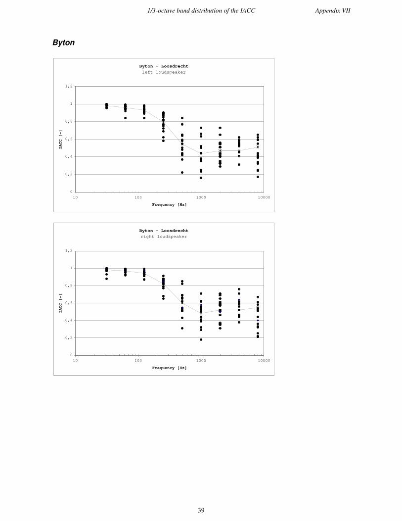
1/3-octave band distribution of the IACC Appendix VII
39
Byton
Byton - Loosdrechtleft loudspeaker
0
0,2
0,4
0,6
0,8
1
1,2
10 100 1000 10000
Frequency [Hz]
IACC [-]
Byton - Loosdrechtright loudspeaker
0
0,2
0,4
0,6
0,8
1
1,2
10 100 1000 10000
Frequency [Hz]
IACC [-]

1/3-octave band distribution of the IACC Appendix VII
40
Frequency [Hz]LEFTLOUDSPEAKER 31.5 63 125 250 500 1000 2000 4000 8000
Receiver 1 1.00 0.98 0.98 0.87 0.84 0.73 0.73 0.56 0.65Receiver 2 1.00 0.99 0.94 0.90 0.77 0.50 0.55 0.54 0.55Receiver 3 0.99 0.98 0.91 0.85 0.65 0.51 0.51 0.53 0.39Receiver 4 0.99 0.94 0.94 0.82 0.48 0.37 0.43 0.45 0.34Receiver 5 0.99 0.95 0.84 0.75 0.22 0.16 0.33 0.31 0.24Receiver 6 0.99 0.97 0.98 0.89 0.58 0.66 0.65 0.62 0.62Receiver 7 0.99 0.99 0.95 0.88 0.65 0.52 0.56 0.58 0.59Receiver 8 0.99 0.98 0.90 0.77 0.64 0.37 0.44 0.59 0.59Receiver 9 0.98 0.97 0.94 0.82 0.43 0.44 0.40 0.53 0.39Receiver 10 0.98 0.92 0.89 0.58 0.42 0.23 0.32 0.41 0.25Receiver 11 0.99 0.94 0.97 0.89 0.37 0.63 0.41 0.58 0.44Receiver 12 0.98 0.97 0.92 0.69 0.55 0.44 0.54 0.55 0.41Receiver 13 0.96 0.99 0.92 0.72 0.50 0.38 0.51 0.52 0.42Receiver 14 0.95 0.98 0.97 0.90 0.59 0.25 0.29 0.45 0.32Receiver 15 0.98 0.84 0.91 0.62 0.44 0.35 0.35 0.45 0.17
Average 0.98 0.96 0.93 0.80 0.54 0.44 0.47 0.47 0.51
Frequency [Hz]RIGHTLOUDSPEAKER 31.5 63 125 250 500 1000 2000 4000 8000
Receiver 1 0.98 0.92 0.92 0.68 0.43 0.41 0.31 0.38 0.22Receiver 2 0.99 0.95 0.91 0.84 0.66 0.56 0.50 0.45 0.21Receiver 3 1.00 0.98 0.96 0.82 0.69 0.53 0.65 0.46 0.44Receiver 4 1.00 0.98 0.99 0.88 0.82 0.62 0.59 0.60 0.61Receiver 5 1.00 0.98 0.96 0.91 0.85 0.71 0.71 0.56 0.67Receiver 6 0.97 0.95 0.91 0.65 0.53 0.32 0.46 0.46 0.25Receiver 7 0.98 0.98 0.87 0.79 0.62 0.39 0.52 0.59 0.36Receiver 8 1.00 0.99 0.94 0.85 0.65 0.55 0.59 0.62 0.54Receiver 9 1.00 0.99 0.97 0.82 0.69 0.52 0.69 0.76 0.53Receiver 10 1.00 0.98 0.96 0.86 0.66 0.62 0.57 0.59 0.58Receiver 11 0.93 0.93 0.96 0.88 0.31 0.18 0.36 0.46 0.21Receiver 12 0.88 0.99 0.93 0.88 0.51 0.29 0.37 0.52 0.32Receiver 13 0.97 0.98 0.91 0.77 0.54 0.44 0.35 0.44 0.33Receiver 14 0.99 0.97 0.95 0.86 0.51 0.50 0.61 0.71 0.51Receiver 15 0.99 0.97 0.97 0.85 0.55 0.58 0.50 0.64 0.40
Average 0.98 0.97 0.94 0.82 0.60 0.48 0.52 0.52 0.55

IACC calculated from different measurement lengths Appendix VIII
41
Appendix VIII: IACC calculated from different measurement lengths
In the tables below the data is presented from the IACC calculations by whereby end of the impulse response isstepwise cut off. This results for every control room in an IACC calculation with a measurement length ofrespectively 1.37 s. (original impulse response). 1.2 s., 1.0 s., 0.8 s., 0.6 s., 0.4 s., 0.2 s. and 0.1 s.
For each control room the data is given in three tables which represent the time intervals of 0 - ∞ ms, 0 – 80 msand 80 - ∞ ms.
Soundbase
Table 2 : IACC calculation results of the same impulse responses with a different measurement length,calculated over the time interval from 0 - ∞∞ ms.
Frequency [Hz]Time [s]31.5 63 125 250 500 1000 2000 4000 8000
1.37 0.97 0.98 0.97 0.57 0.49 0.68 0.70 0.67 0.371.20 0.97 0.98 0.97 0.57 0.49 0.68 0.70 0.67 0.371.00 0.97 0.98 0.97 0.57 0.49 0.68 0.70 0.67 0.370.80 0.97 0.98 0.97 0.57 0.49 0.68 0.70 0.67 0.370.60 0.97 0.98 0.97 0.57 0.49 0.68 0.70 0.67 0.370.40 0.97 0.98 0.97 0.57 0.49 0.68 0.70 0.67 0.370.20 0.97 0.98 0.97 0.57 0.49 0.68 0.70 0.67 0.370.10 0.97 0.98 0.97 0.57 0.49 0.68 0.70 0.67 0.37
Table 3 : IACC calculation results of the same impulse responses with a different measurement length,calculated over the time interval from 80 - ∞∞ ms.
Frequency [Hz]Time [s]31.5 63 125 250 500 1000 2000 4000 8000
1.37 0.91 0.96 0.95 0.67 0.41 0.29 0.21 0.10 0.111.20 0.91 0.96 0.95 0.67 0.41 0.29 0.21 0.09 0.111.00 0.91 0.96 0.95 0.67 0.41 0.29 0.21 0.09 0.110.80 0.91 0.96 0.96 0.68 0.42 0.29 0.22 0.10 0.110.60 0.91 0.96 0.96 0.69 0.43 0.28 0.23 0.11 0.100.40 0.91 0.96 0.96 0.69 0.43 0.29 0.23 0.12 0.110.20 0.91 0.96 0.96 0.69 0.43 0.29 0.24 0.14 0.110.10 0.83 0.92 0.96 0.77 0.69 0.31 0.39 0.21 0.21

IACC calculated from different measurement lengths Appendix VIII
42
JVPS
Table 4 : IACC calculation results of the same impulse responses with a different measurement length,calculated over the time interval from 0 - ∞∞ ms.
Frequency [Hz]Time [s]31.5 63 125 250 500 1000 2000 4000 8000
1.37 0.99 0.99 0.95 0.92 0.71 0.68 0.67 0.56 0.231.20 0.99 0.99 0.95 0.92 0.71 0.68 0.67 0.56 0.231.00 0.99 0.99 0.95 0.92 0.71 0.68 0.67 0.56 0.230.80 0.99 0.99 0.95 0.92 0.71 0.68 0.67 0.56 0.230.60 0.99 0.99 0.95 0.92 0.71 0.68 0.67 0.56 0.230.40 0.99 0.99 0.95 0.92 0.71 0.68 0.67 0.56 0.230.20 0.99 0.99 0.95 0.92 0.71 0.68 0.67 0.56 0.230.10 1.00 0.99 0.96 0.92 0.71 0.68 0.67 0.56 0.23
Table 5 : IACC calculation results of the same impulse responses with a different measurement length,calculated over the time interval from 80 - ∞∞ ms.
Frequency [Hz]Time [s]31.5 63 125 250 500 1000 2000 4000 8000
1.37 0.91 0.94 0.89 0.47 0.35 0.33 0.16 0.18 0.061.20 0.91 0.94 0.89 0.47 0.35 0.33 0.17 0.17 0.071.00 0.91 0.94 0.89 0.47 0.35 0.34 0.17 0.17 0.070.80 0.91 0.94 0.89 0.47 0.36 0.35 0.18 0.16 0.070.60 0.91 0.94 0.89 0.47 0.37 0.35 0.20 0.16 0.070.40 0.91 0.94 0.89 0.48 0.37 0.36 0.21 0.15 0.070.20 0.91 0.94 0.89 0.48 0.38 0.36 0.24 0.14 0.070.10 0.19 0.96 0.86 0.71 0.51 0.56 0.56 0.21 0.25

IACC calculated from different measurement lengths Appendix VIII
43
Topsound
Table 6 : IACC calculation results of the same impulse responses with a different measurement length,calculated over the time interval from 0 - ∞∞ ms.
Frequency [Hz]Time [s]31.5 63 125 250 500 1000 2000 4000 8000
1.37 0.99 0.99 0.95 0.79 0.88 0.65 0.45 0.42 0.371.20 0.99 0.99 0.95 0.79 0.88 0.65 0.45 0.42 0.371.00 0.99 0.99 0.95 0.79 0.88 0.65 0.45 0.42 0.370.80 0.99 0.99 0.95 0.79 0.88 0.65 0.45 0.42 0.370.60 0.99 0.99 0.95 0.79 0.88 0.65 0.45 0.42 0.370.40 0.99 0.99 0.95 0.79 0.88 0.65 0.45 0.42 0.370.20 0.99 0.99 0.95 0.79 0.88 0.65 0.45 0.42 0.370.10 0.99 0.99 0.95 0.79 0.88 0.65 0.45 0.42 0.37
Table 7 : IACC calculation results of the same impulse responses with a different measurement length,calculated over the time interval from 80 - ∞∞ ms.
Frequency [Hz]Time [s]31.5 63 125 250 500 1000 2000 4000 8000
1.37 0.92 0.99 0.86 0.77 0.07 0.23 0.14 0.09 0.051.20 0.87 0.98 0.95 0.26 0.5 0.43 0.32 0.2 0.141.00 0.93 0.99 0.88 0.55 0.22 0.35 0.21 0.16 0.070.80 0.92 0.99 0.88 0.68 0.16 0.32 0.19 0.14 0.060.60 0.92 0.99 0.87 0.69 0.12 0.29 0.18 0.13 0.050.40 0.92 0.99 0.87 0.72 0.10 0.27 0.17 0.12 0.050.20 0.92 0.99 0.87 0.75 0.08 0.25 0.15 0.11 0.050.10 0.92 0.99 0.86 0.76 0.07 0.23 0.14 0.1 0.05

IACC calculated from different measurement lengths Appendix VIII
44
Ferry & Garnefski
Table 8 : IACC calculation results of the same impulse responses with a different measurement length,calculated over the time interval from 0 - ∞∞ ms.
Frequency [Hz]Time [s]31.5 63 125 250 500 1000 2000 4000 8000
1.37 0.95 0.99 0.99 0.96 0.81 0.84 0.53 0.55 0.321.20 0.95 0.99 0.99 0.96 0.81 0.84 0.53 0.55 0.321.00 0.96 0.99 0.99 0.96 0.81 0.84 0.53 0.55 0.320.80 0.96 0.99 0.99 0.96 0.81 0.84 0.53 0.55 0.320.60 0.97 0.99 0.99 0.96 0.81 0.84 0.53 0.55 0.320.40 0.97 0.99 0.99 0.96 0.81 0.84 0.53 0.55 0.320.20 0.97 0.99 0.99 0.96 0.81 0.84 0.53 0.55 0.320.10 0.97 0.99 0.99 0.96 0.81 0.84 0.53 0.55 0.32
Table 9 : IACC calculation results of the same impulse responses with a different measurement length,calculated over the time interval from 80 - ∞∞ ms.
Frequency [Hz]Time [s]31.5 63 125 250 500 1000 2000 4000 8000
1.37 0.86 0.93 0.94 0.61 0.46 0.32 0.37 0.12 0.061.20 0.85 0.94 0.94 0.62 0.45 0.3 0.37 0.12 0.061.00 0.85 0.94 0.94 0.65 0.43 0.27 0.37 0.13 0.070.80 0.88 0.94 0.94 0.65 0.41 0.26 0.36 0.14 0.070.60 0.91 0.95 0.94 0.65 0.35 0.25 0.36 0.15 0.080.40 0.89 0.95 0.94 0.69 0.26 0.24 0.36 0.15 0.10.20 0.94 0.96 0.95 0.77 0.23 0.24 0.36 0.17 0.110.10 0.99 0.9 0.93 0.83 0.45 0.33 0.41 0.24 0.17

IACC calculated from different measurement lengths Appendix VIII
45
Soundhouse
Table 10 : IACC calculation results of the same impulse responses with a different measurement length,calculated over the time interval from 0 - ∞∞ ms.
Frequency [Hz]Time [s]31.5 63 125 250 500 1000 2000 4000 8000
1.37 0.99 0.98 0.94 0.82 0.36 0.41 0.56 0.65 0.401.20 0.99 0.98 0.94 0.82 0.36 0.41 0.56 0.65 0.401.00 0.99 0.98 0.94 0.82 0.36 0.41 0.56 0.65 0.400.80 0.99 0.98 0.94 0.82 0.36 0.41 0.56 0.65 0.400.60 0.99 0.98 0.94 0.82 0.36 0.41 0.56 0.65 0.400.40 0.99 0.98 0.94 0.82 0.36 0.41 0.56 0.65 0.400.20 0.99 0.98 0.94 0.82 0.36 0.41 0.56 0.65 0.400.10 1.00 0.98 0.94 0.82 0.37 0.42 0.57 0.66 0.40
Table 11 : IACC calculation results of the same impulse responses with a different measurement length,calculated over the time interval from 80 - ∞∞ ms.
Frequency [Hz]Time [s]31.5 63 125 250 500 1000 2000 4000 8000
1.37 0.97 0.98 0.95 0.66 0.28 0.38 0.11 0.15 0.101.20 0.97 0.98 0.95 0.66 0.28 0.38 0.11 0.15 0.101.00 0.97 0.98 0.95 0.66 0.28 0.38 0.11 0.15 0.100.80 0.97 0.98 0.95 0.66 0.28 0.38 0.11 0.15 0.100.60 0.97 0.98 0.95 0.66 0.28 0.38 0.11 0.15 0.100.40 0.97 0.98 0.95 0.66 0.28 0.38 0.11 0.15 0.100.20 0.98 0.98 0.95 0.67 0.28 0.39 0.11 0.15 0.100.10 0.99 0.90 0.97 0.79 0.47 0.74 0.32 0.23 0.18

IACC calculated from different measurement lengths Appendix VIII
46
Byton
Table 12 : IACC calculation results of the same impulse responses with a different measurement length,calculated over the time interval from 0 - ∞∞ ms.
Frequency [Hz]Time [s]31.5 63 125 250 500 1000 2000 4000 8000
1.37 0.99 0.98 0.9 0.77 0.64 0.37 0.44 0.59 0.591.20 0.99 0.98 0.9 0.77 0.64 0.37 0.44 0.59 0.591.00 0.99 0.98 0.9 0.77 0.64 0.37 0.44 0.59 0.590.80 0.99 0.98 0.9 0.77 0.64 0.37 0.44 0.59 0.590.60 0.99 0.98 0.9 0.77 0.64 0.37 0.44 0.59 0.590.40 0.99 0.98 0.9 0.77 0.64 0.37 0.44 0.59 0.590.20 0.99 0.98 0.9 0.77 0.64 0.37 0.44 0.59 0.590.10 0.99 0.98 0.9 0.77 0.64 0.37 0.44 0.59 0.59
Table 13 : IACC calculation results of the same impulse responses with a different measurement length,calculated over the time interval from 80 - ∞∞ ms.
Frequency [Hz]Time [s]31.5 63 125 250 500 1000 2000 4000 8000
1.37 0.94 0.98 0.88 0.82 0.27 0.15 0.16 0.21 0.131.20 0.94 0.98 0.88 0.83 0.27 0.15 0.16 0.21 0.131.00 0.95 0.98 0.89 0.83 0.27 0.15 0.16 0.21 0.130.80 0.95 0.98 0.89 0.83 0.27 0.15 0.16 0.21 0.130.60 0.95 0.98 0.89 0.83 0.27 0.15 0.16 0.21 0.130.40 0.95 0.98 0.89 0.83 0.27 0.15 0.16 0.21 0.130.20 0.95 0.98 0.89 0.83 0.27 0.15 0.16 0.21 0.130.10 0.96 0.98 0.81 0.85 0.35 0.32 0.34 0.28 0.21

Reverberation times in control rooms Appendix IX
47
Appendix IX: Reverberation times in control rooms
In the figures below the reverberation times which have been measured in the control rooms under test arepresented. The curves show the recommended ITU reverberation limits, the maximum and minimum measuredvalues in the grid and the averaged results. Below the curves the actual data is presented in a table.
All data is gathered from measurements with the omni directional microphone, except the data of theSoundhouse control room. Due to a low signal-to-noise ratio the data below 500 Hz was unreliable. Comparisonbetween the different microphones justified the substitution of the omni directional microphone by themeasurement result of the artificial head (see paragraph 4.6.3. of the main document).
Soundbase
Soundbase - Groningen Left loudspeaker
0
0,1
0,2
0,3
0,4
0,5
0,6
10 100 1000 10000
Frequency [Hz]
T30 [s]
ITU limit Min / max Average
Soundbase - GroningenRight loudspeaker
0
0,1
0,2
0,3
0,4
0,5
0,6
10 100 1000 10000
Frequency [Hz]
T30 [s]
ITU limit Min / max Average
Table 14 : Measured reverberation times (T30 [s]) in the Soundbase control room.
Left loudspeaker Right loudspeakerFrequency
[Hz]Minimum Maximum Average Minimum Maximum Average
63 0.24 0.56 0.47 0.39 0.52 0.46125 0.26 0.36 0.31 0.25 0.33 0.30250 0.17 0.24 0.21 0.18 0.24 0.22500 0.19 0.23 0.22 0.20 0.25 0.221000 0.17 0.21 0.19 0.16 0.19 0.182000 0.17 0.19 0.18 0.15 0.18 0.174000 0.14 0.16 0.15 0.13 0.15 0.148000 0.13 0.14 0.14 0.11 0.14 0.13

Reverberation times in control rooms Appendix IX
48
JVPS
Jay Vandenberg's Private Studio - EnschedeLeft loudspeaker
0
0,1
0,2
0,3
0,4
0,5
0,6
10 100 1000 10000
Frequency [Hz]
T30 [s]
ITU limit Min / max Average
Jay Vandenberg's Private Studio - EnschedeRight loudspeaker
0
0,1
0,2
0,3
0,4
0,5
0,6
10 100 1000 10000
Frequency [Hz]
T30 [s]
ITU limit Min / max Average
Table 15 : Measured reverberation times (T30 [s]) in the JVPS control room.
Left loudspeaker Right loudspeakerFrequency
[Hz]Minimum Maximum Average Minimum Maximum Average
63 0.18 0.47 0.35 0.26 0.47 0.38125 0.19 0.27 0.23 0.15 0.25 0.20250 0.16 0.20 0.19 0.15 0.20 0.19500 0.17 0.22 0.21 0.17 0.23 0.201000 0.20 0.23 0.21 0.18 0.23 0.212000 0.20 0.25 0.21 0.20 0.22 0.214000 0.20 0.22 0.21 0.20 0.21 0.208000 0.18 0.20 0.19 0.17 0.20 0.19

Reverberation times in control rooms Appendix IX
49
Topsound
Topsound - EnschedeLeft loudspeaker
0
0,1
0,2
0,3
0,4
0,5
0,6
10 100 1000 10000
Frequency [Hz]
T30 [s]
ITU limit Min / max Average
Topsound - EnschedeRight loudspeaker
0
0,1
0,2
0,3
0,4
0,5
0,6
10 100 1000 10000
Frequency [Hz]
T30 [s]
ITU limit Min / max Average
Table 16 : Measured reverberation times (T30 [s]) in the Topsound control room.
Left loudspeaker Right loudspeaker
Frequency[Hz]
Minimum Maximum Average Minimum Maximum Average
63 0.25 0.40 0.35 0.25 0.40 0.34125 0.17 0.31 0.26 0.19 0.33 0.26250 0.16 0.22 0.19 0.15 0.30 0.20500 0.11 0.16 0.14 0.13 0.16 0.141000 0.13 0.16 0.15 0.13 0.16 0.142000 0.13 0.16 0.14 0.13 0.15 0.144000 0.12 0.14 0.13 0.12 0.15 0.148000 0.11 0.13 0.12 0.11 0.13 0.12

Reverberation times in control rooms Appendix IX
50
Ferry & Garnefski
Ferry & Garnefski - AmsterdamLeft loudspeaker
0
0,1
0,2
0,3
0,4
0,5
0,6
10 100 1000 10000
Frequency [Hz]
T30 [s]
ITU limit Min / max Average
Ferry & Garnefski - AmsterdamRight loudspeaker
0
0,1
0,2
0,3
0,4
0,5
0,6
10 100 1000 10000
Frequency [Hz]
T30 [s]
ITU limit Min / max Average
Table 17 : Measured reverberation times (T30 [s]) in the Ferry & Garnefski control room.
Left loudspeaker Right loudspeakerFrequency
[Hz]Minimum Maximum Average Minimum Maximum Average
63 0.08 0.49 0.26 0.16 0.40 0.25125 0.04 0.38 0.15 0.06 0.24 0.16250 0.09 0.18 0.13 0.05 0.16 0.12500 0.10 0.16 0.13 0.13 0.16 0.141000 0.11 0.16 0.14 0.04 0.17 0.132000 0.12 0.16 0.15 0.10 0.16 0.144000 0.13 0.16 0.14 0.09 0.17 0.148000 0.13 0.15 0.14 0.09 0.15 0.14

Reverberation times in control rooms Appendix IX
51
Soundhouse
Soundhouse - SchiedamLeft loudspeaker
0
0,1
0,2
0,3
0,4
0,5
0,6
0,7
0,8
10 100 1000 10000
Frequency [Hz]
T30 [s]
ITU limit Min / max Average
Soundhouse - SchiedamRight loudspeaker
0
0,1
0,2
0,3
0,4
0,5
0,6
10 100 1000 10000
Frequency [Hz]
T30 [s]
ITU limit Min / max Average
Table 18 : Measured reverberation times (T30 [s]) in the Soundhouse control room.
Left loudspeaker Right loudspeakerFrequency
[Hz]Minimum Maximum Average Minimum Maximum Average
63 0.27 0.73 0.41 0.30 0.52 0.38125 0.24 0.37 0.30 0.21 0.37 0.29250 0.23 0.37 0.29 0.24 0.35 0.29500 0.29 0.39 0.34 0.30 0.42 0.351000 0.31 0.41 0.36 0.32 0.38 0.352000 0.35 0.40 0.37 0.36 0.42 0.384000 0.35 0.41 0.38 0.32 0.40 0.368000 0.29 0.34 0.31 0.27 0.33 0.30

Reverberation times in control rooms Appendix IX
52
Byton
Byton - LoosdrechtLeft loudspeaker
0
0,1
0,2
0,3
0,4
0,5
0,6
0,7
10 100 1000 10000
Frequency [Hz]
T30 [s]
ITU limit Min / max Average
Byton - LoosdrechtRight loudspeaker
0
0,1
0,2
0,3
0,4
0,5
0,6
0,7
10 100 1000 10000
Frequency [Hz]
T30 [s]
ITU limit Min / max Average
Table 19 : Measured reverberation times (T30 [s]) in the Byton control room.
Left loudspeaker Right loudspeakerFrequency
[Hz]Minimum Maximum Average Minimum Maximum Average
63 0.33 0.58 0.44 0.36 0.63 0.45125 0.30 0.38 0.33 0.29 0.42 0.35250 0.23 0.29 0.26 0.20 0.29 0.25500 0.20 0.24 0.22 0.20 0.30 0.231000 0.21 0.26 0.24 0.22 0.28 0.242000 0.22 0.26 0.24 0.22 0.27 0.244000 0.21 0.26 0.23 0.21 0.26 0.228000 0.20 0.24 0.21 0.20 0.24 0.22

Low frequent rms-values at the engineer positions Appendix X
53
Appendix X: Low frequency rms-values at the engineer positions
The figures below present the rms-values calculated for the lower 1/3-octave frequency bands in each controlroom, excitated with respectively the left and right loudspeaker. All the figures concern the designed engineerposition, i.e. position eight according to the grid. The upper graphs present the control rooms designed by BenKok, i.e. Byton, Ferry & Garnefski and Soundhouse. The lower curves present the control rooms designed byAlex Balster, i.e. JVPS2, Topsound and Soundbase.
The frequency bands are indicated with bandnumbers. From the table below the bandnumber and the accessoryfrequency band can be obtained.
Table 20 : Bandnumbers and accessory frequency bands which are used in the graphs.
Bandnumber Frequency band [Hz]1 25 – 322 32 – 403 40 – 504 50 – 635 63 – 806 80 – 1007 125 – 1608 160 – 2009 200 – 250
Figure 20 : Rms-column diagrams for the control rooms under test, excitated by the left loudspeaker.
2 Here the JVPS control room is indicated with Hitbox. This was the name the control room used to have.

Low frequent rms-values at the engineer positions Appendix X
54
Figure 21: Rms-column diagrams for the control rooms under test, excitated by the right loudspeaker.

55