Electronic copy available at: http://ssrn.com/abstract=2024716

Beyond Q:

Estimating Investment without Asset Prices

Vito D. Gala and Joao Gomes∗

June 5, 2012

Abstract

Empirical corporate finance studies often rely on measures of Tobin’s Q to con-

trol for “fundamental” determinants of investment. However, since Tobin’s Q is a

good summary of investment behavior only under very stringent conditions, it is far

better to instead use the underlying state variables directly. In this paper we show

that under very general assumptions about the nature of technology and markets,

these state variables are easily measurable and greatly improve the empirical fit of

investment models. Even a general first or second order polynomial that does not

rely on additional details about the nature of the investment problem accounts for

a substantially larger fraction of the total variation in corporate investment than

standard Q measures.

Keywords: Investment, Firm Size, Tobin’s Q.

∗Vito D. Gala is at London Business School, vgala@london.edu; Joao Gomes is at The WhartonSchool of the University of Pennsylvania, gomesj@wharton.upenn.edu. We thank seminar participantsat various institutions for valuable comments and suggestions. All errors are our own.

1

Electronic copy available at: http://ssrn.com/abstract=2024716

Hayashi’s (1982) famous elaboration of Brainard and Tobin’s Q-theory has influenced

the theory and practice of corporate and aggregate investment for nearly three decades.

The prediction that Tobin’s Q is a sufficient statistic to describe investment behavior

has proved immensely popular among researchers, and the simple investment regressions

implied by the linear-quadratic versions of the model form the basis for a myriad of

empirical studies in economics and finance. Despite a long-standing consensus that Q is

poorly measured and that the homogenous linear-quadratic model which motivates its

use is misspecified, linear Q-based investment regressions still form the basis for most of

inferences about corporate behaviors.1 This practice is even harder to justify on empirical

grounds since Tobin’s Q accounts for very little of the variation in firm level investment.

In this paper we propose an alternative procedure to estimate investment equations

under very general assumptions about the nature of technology and markets. Our

methodology is not only superior theoretically and empirically, but also easier to im-

plement and even applicable to private firms. Like others, our starting point is also a

structural model of corporate investment behavior, but without the usual often counter-

factual assumptions about homogeneity and perfect competition.2 We exploit the fact

that the optimal investment policy is always function of key state variables of the firm

and can be approximated by a low order polynomial. Unlike marginal q, many of the

state variables are directly observable or can be readily constructed from observables,

under fairly general conditions.

Empirically, the main novelty of our approach is to identify firm size and sales (or

cash flows) as the key state variables for optimal investment. Surprisingly, given its

popularity in other empirical applications, firm size is often ignored in the investment

literature, and if used, it usually shows up only as sorting variable for identification of

1Q-based investment regressions, often augmented by various ad-hoc measures of cash flows, havebeen used to, among other purposes, test the importance of financial constraints, the effects of corporategovernance, the consequences of having bad CEOs and the efficiency of market of signals.

2Possible departures from homogeneity due to technological and/or financial frictions include marketpower or decreasing returns to scale in production (Gomes, 2001; Cooper and Ejarque, 2003; Abel andEberly, 2010), inhomogeneous costs of investment (Abel and Eberly, 1994, 1997; Cooper and Haltiwanger,2006), and inhomogeneous costs of external financing (Hennessy and Whited, 2007).

Electronic copy available at: http://ssrn.com/abstract=2024716

financially constrained firms.3 We show, instead, that firm size naturally becomes an

important determinant of investment whenever Tobin’s Q is not a sufficient statistic,

even in the absence of financial market frictions.

Our approach also clarifies the role of sales or cash flow variables. Contrary to the

once popular use of these variables in tests of financing constraints, we show that they

matter because they capture shocks to productivity and demand as well as any variations

in factor prices. This interpretation is also suggested in Gomes (2001), and Cooper

and Ejarque (2003), while Abel and Eberly (2010) focus instead on differences between

marginal and average Q. In those studies however, the role of cash flow is often limited to

rationalize the evidence based on misspecified Q-type investment regressions, and often

considered marginal relative to Tobin’s Q. Instead, we argue that cash flow or sales should

always be treated as a primary determinant of investment, regardless of Tobin’s Q, and

even in the absence of capital market imperfections.

An important corollary of our paper is that investment can be studied without us-

ing market values. As a result, our methodology can be readily applied to study the

behavior of private as well as public firms. As data on private firms is becoming more

widely available this provides a significant advantage over existing Q-theory.4 By avoiding

market values we also minimize the serious measurement concerns induced by potential

stock market misvaluations (Blanchard, Rhee and Summers, 1993; Erickson and Whited,

2000), and approximations of unavailable market values of debt securities. No doubt

many of our proposed variables are also subject to measurement error, but this is likely

to be far smaller than in Tobin’s Q.

Empirically, our state variable representation of the optimal investment policy is

noticeably superior to that of standard Q-type investment regressions. Both firm size

and sales account for more than twice as much as Tobin’s Q of the within-variation

in investment, and more than four times as much as Tobin’s Q of the total explained

investment variation. The empirical performance is even stronger in first differences: our

3A notable exception is Gala and Julio (2011).4Asker, Farre-Mensa and Ljungqvist (2011) offer an example on the difficulties of using Q-theory

with non-traded firms.

2

core state variables can explain as much as eight times more than Tobin’s Q of the overall

variation in investment changes, and account for about 96 percent of the total explained

variation in investment changes.

Finally, although we focus mainly on frictionless investment models, our approach can

easily accommodate financial frictions. Intuitively, most deviations from the Modigliani-

Miller theorem imply that the optimal investment policy often depends on an augmented

set of state variables, which also includes financial leverage. We show how to pursue

this extension by including different measures of financial leverage as state variables, in

addition to firm size and sales. Similarly, we show how our methodology can easily handle

more complex adjustment cost specifications like in Eberly, Rebelo and Vincent (2011),

by including lagged investment as additional state variable for the optimal investment

policy. Our polynomial approximation approach can also account for the impact of

aggregate variation on investment, above and beyond the variation already incorporated

in the measured firm level state variables, by augmenting the polynomial state variables

with a complete set of time dummies.

In many ways our paper follows logically from the work of Erickson andWhited (2000,

2006 and 2011) and their ultimate conclusion that “Tobin’s Q contains a great deal of

measurement error because of a conceptual gap between true investment opportunities

and observable measures”. Our suggestion here is to simply avoid the notoriously dif-

ficult problem of treating measurement error in the market value of a firm’s assets and

limit any potential errors to the measurement of the firm’s capital stock, which contains

substantially less noise (Erickson and Whited, 2006, 2011).

We believe our paper contributes to the literature in three significant ways. First,

and foremost, it provides a superior empirical methodology to characterize firm level

investment behavior. With a better empirical description at hand, we are able to quantify

through a statistical variance decomposition the importance of various state variables,

and corresponding class of investment models, for the overall variation in investment.

Second, we provide a clearly articulated justification for the use of firm size as well

as alternative flow variables, such as sales and operating profits, as determinants of

3

investment. Although the latter are often informally motivated, there are very few formal

arguments in the context of a very general investment model. Third, unlike misspecified

Q-type investment regressions, our direct approximation of investment provides naturally

more informative empirical moments for the identification and inference of the underlying

structural parameters of the model. This is particularly useful for estimation of structural

models via indirect inference methods.

The rest of our paper is organized as follows. The next section describes our gen-

eral model, the implied optimal investment policies, and how they can be approximated

empirically as function of the key state variables. We describe the data in Section 3,

and present the main findings in Section III.. We discuss how to generalize the basic

approach to accommodate labor market shocks, capital markets imperfections and alter-

native adjustment cost specifications in Section IV.. We conclude in Section V. with a

brief discussion of the role of asset prices in estimating investment.

I. Modeling Investment

This section describes the general structural model of corporate investment that we use

in our empirical work. To both clarify and emphasize the exact differences with respect

to the more restrictive Q-theory environments, we need to be explicit about our detailed

assumptions. We use a version of the general model in Abel and Eberly (1994, 1997)

which allows for asymmetric, non-convex and possibly discontinuous adjustment costs,

together with a general weakly concave technology that allows for decreasing returns to

scale. We believe that this environment is flexible enough to include the large majority

of investment models in the literature as special cases. For exposition purposes, we delay

the introduction of additional features such as financial market imperfections, which are

instead discussed in Section 5.

4

A. The General Model

We start by examining the optimal investment decision of a firm that seeks to maximize

current shareholder value in the absence of any financing frictions, V . For simplicity, we

assume that the firm is financed entirely by equity and denote by D the value of periodic

distributions net of any securities issuance.

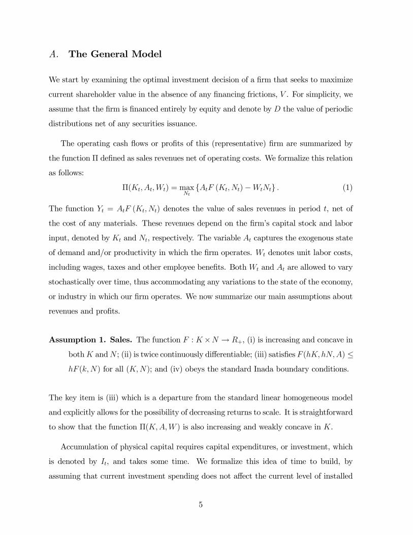
The operating cash flows or profits of this (representative) firm are summarized by

the function Π defined as sales revenues net of operating costs. We formalize this relation

as follows:

Π(Kt, At,Wt) = maxNt

AtF (Kt, Nt)−WtNt . (1)

The function Yt = AtF (Kt, Nt) denotes the value of sales revenues in period t, net of

the cost of any materials. These revenues depend on the firm’s capital stock and labor

input, denoted by Kt and Nt, respectively. The variable At captures the exogenous state

of demand and/or productivity in which the firm operates. Wt denotes unit labor costs,

including wages, taxes and other employee benefits. Both Wt and At are allowed to vary

stochastically over time, thus accommodating any variations to the state of the economy,

or industry in which our firm operates. We now summarize our main assumptions about

revenues and profits.

Assumption 1. Sales. The function F : K×N → R+, (i) is increasing and concave in

bothK andN ; (ii) is twice continuously differentiable; (iii) satisfies F (hK, hN,A) ≤

hF (k,N) for all (K,N); and (iv) obeys the standard Inada boundary conditions.

The key item is (iii) which is a departure from the standard linear homogeneous model

and explicitly allows for the possibility of decreasing returns to scale. It is straightforward

to show that the function Π(K,A,W ) is also increasing and weakly concave in K.

Accumulation of physical capital requires capital expenditures, or investment, which

is denoted by It, and takes some time. We formalize this idea of time to build, by

assuming that current investment spending does not affect the current level of installed

5

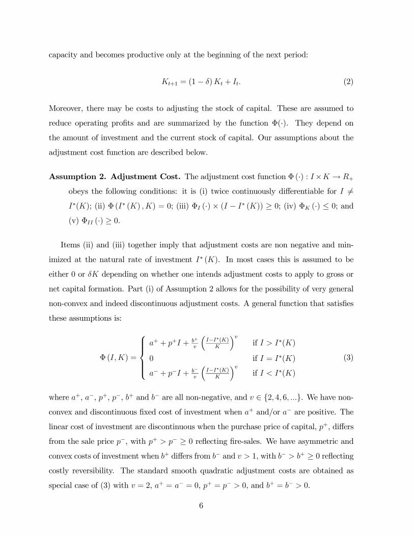
capacity and becomes productive only at the beginning of the next period:

Kt+1 = (1− δ)Kt + It. (2)

Moreover, there may be costs to adjusting the stock of capital. These are assumed to

reduce operating profits and are summarized by the function Φ(·). They depend on

the amount of investment and the current stock of capital. Our assumptions about the

adjustment cost function are described below.

Assumption 2. Adjustment Cost. The adjustment cost function Φ (·) : I×K → R+

obeys the following conditions: it is (i) twice continuously differentiable for I 6=

I∗(K); (ii) Φ (I∗ (K) ,K) = 0; (iii) ΦI (·) × (I − I∗ (K)) ≥ 0; (iv) ΦK (·) ≤ 0; and

(v) ΦII (·) ≥ 0.

Items (ii) and (iii) together imply that adjustment costs are non negative and min-

imized at the natural rate of investment I∗ (K). In most cases this is assumed to be

either 0 or δK depending on whether one intends adjustment costs to apply to gross or

net capital formation. Part (i) of Assumption 2 allows for the possibility of very general

non-convex and indeed discontinuous adjustment costs. A general function that satisfies

these assumptions is:

Φ (I,K) =

⎧⎪⎪⎪⎨⎪⎪⎪⎩a+ + p+I + b+

v

³I−I∗(K)

K

´vif I > I∗(K)

0 if I = I∗(K)

a− + p−I + b−

v

³I−I∗(K)

K

´vif I < I∗(K)

(3)

where a+, a−, p+, p−, b+ and b− are all non-negative, and v ∈ 2, 4, 6, .... We have non-

convex and discontinuous fixed cost of investment when a+ and/or a− are positive. The

linear cost of investment are discontinuous when the purchase price of capital, p+, differs

from the sale price p−, with p+ > p− ≥ 0 reflecting fire-sales. We have asymmetric and

convex costs of investment when b+ differs from b− and v > 1, with b− > b+ ≥ 0 reflecting

costly reversibility. The standard smooth quadratic adjustment costs are obtained as

special case of (3) with v = 2, a+ = a− = 0, p+ = p− > 0, and b+ = b− > 0.

6

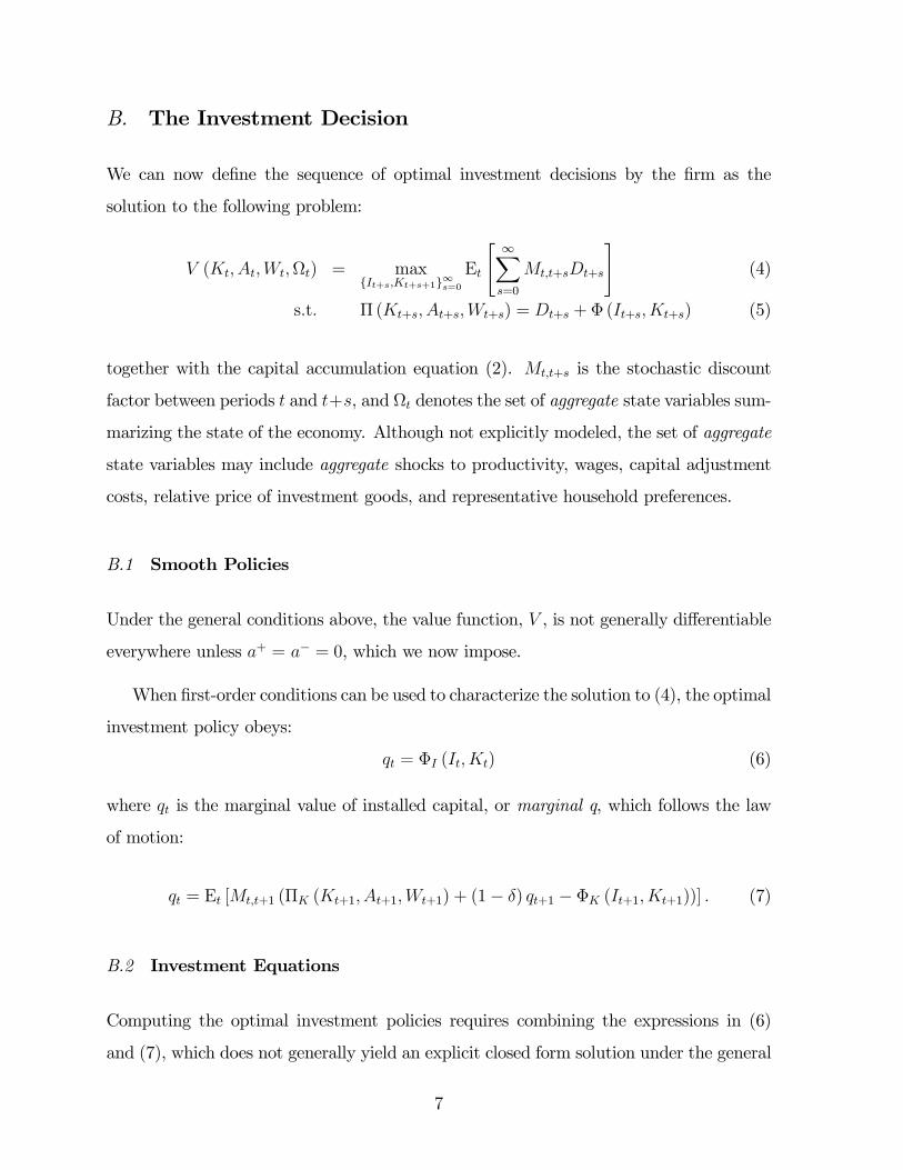
B. The Investment Decision

We can now define the sequence of optimal investment decisions by the firm as the

solution to the following problem:

V (Kt, At,Wt,Ωt) = maxIt+s,Kt+s+1∞s=0

Et

" ∞Xs=0

Mt,t+sDt+s

#(4)

s.t. Π (Kt+s, At+s,Wt+s) = Dt+s + Φ (It+s,Kt+s) (5)

together with the capital accumulation equation (2). Mt,t+s is the stochastic discount

factor between periods t and t+s, and Ωt denotes the set of aggregate state variables sum-

marizing the state of the economy. Although not explicitly modeled, the set of aggregate

state variables may include aggregate shocks to productivity, wages, capital adjustment

costs, relative price of investment goods, and representative household preferences.

B.1 Smooth Policies

Under the general conditions above, the value function, V , is not generally differentiable

everywhere unless a+ = a− = 0, which we now impose.

When first-order conditions can be used to characterize the solution to (4), the optimal

investment policy obeys:

qt = ΦI (It, Kt) (6)

where qt is the marginal value of installed capital, or marginal q, which follows the law

of motion:

qt = Et [Mt,t+1 (ΠK (Kt+1, At+1,Wt+1) + (1− δ) qt+1 − ΦK (It+1,Kt+1))] . (7)

B.2 Investment Equations

Computing the optimal investment policies requires combining the expressions in (6)

and (7), which does not generally yield an explicit closed form solution under the general

7

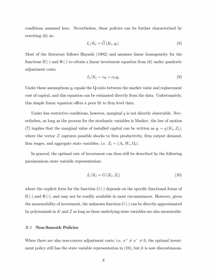
conditions assumed here. Nevertheless, these policies can be further characterized by

rewriting (6) as:

It/Kt = eG (Kt, qt) . (8)

Most of the literature follows Hayashi (1982) and assumes linear homogeneity for the

functions Π (·) and Φ (·) to obtain a linear investment equation from (6) under quadratic

adjustment costs:

It/Kt = α0 + α1qt. (9)

Under these assumptions qt equals the Q-ratio between the market value and replacement

cost of capital, and this equation can be estimated directly from the data. Unfortunately,

this simple linear equation offers a poor fit to firm level data.

Under less restrictive conditions, however, marginal q is not directly observable. Nev-

ertheless, as long as the process for the stochastic variables is Markov, the law of motion

(7) implies that the marginal value of installed capital can be written as qt = q (Kt, Zt),

where the vector Z captures possible shocks to firm productivity, firm output demand,

firm wages, and aggregate state variables, i.e. Zt = (At,Wt,Ωt).

In general, the optimal rate of investment can then still be described by the following

parsimonious state variable representation:

It/Kt = G (Kt, Zt) (10)

where the explicit form for the function G (·) depends on the specific functional forms of

Π (·) and Φ (·), and may not be readily available in most circumstances. However, given

the measurability of investment, the unknown functionG (·) can be directly approximated

by polynomials inK and Z as long as these underlying state variables are also measurable.

B.3 Non-Smooth Policies

When there are also non-convex adjustment costs, i.e. a+ 6= a− 6= 0, the optimal invest-

ment policy still has the state variable representation in (10), but it is now discontinuous.

8

In this case, the optimal investment policy may either be estimated in two branches, to-

gether with the endogenous point of discontinuity, or we may require several higher order

polynomial terms to better capture the nonlinearities. We choose the latter to preserve

uniformity in the presentation.5

C. Our Estimation Approach

Given the widely acknowledged failure of simple linear models, some authors have pro-

posed slightly modified versions of equation (10) by relaxing some assumptions about

technology and costs. This approach has often yielded improved results, but has gener-

ally remained close to the basic linear model.

Instead of imposing additional conditions beyond those in Assumptions 1 and 2,

we choose instead to approximate globally the general investment equation by using a

polynomial version of the general function G(K,Z). Specifically, the approximate tensor

product representation for the optimal investment policy is:

I

K'

nkXik=0

nzXiz=0

cik,izkikziz (11)

where z = log (Z) and k = log (K). We estimate the coefficients cik,iz via ordinary least

squares approximation. These coefficients can then be used to further infer the underlying

structural parameters of the model, for instance using indirect inference methods, or at

the very least, place restrictions on the nature of technology and adjustment costs.

Several practical questions arise when implementing these approximations in empirical

work. The first issue concerns the order of the polynomial. As shown below, in most

cases we find that a second order polynomial in k and z is often sufficient, and higher

order terms are generally not necessary to improve the quality of the approximation.

Practically, we focus on tensor product polynomials of second order in k and z.

5More generally, the optimal investment policy can also be estimated using a full non-parametricapproach.

9

A related issue is whether to use natural or orthogonal polynomial terms in the

approximation. We find that empirical estimates generally work better when we use

orthogonal polynomials. Indeed, when using higher order polynomials multicollinearity

can become a problem when attempting to obtain precise estimates for the parameters

cik,iz . However, the use of orthogonal polynomials makes it more difficult to interpret

the estimated coefficients and also to establish a link to the underlying structural model.

Since we prefer to emphasize the overall fit of our model and are less concerned about

the significance of individual coefficients, we report only the results based on natural

polynomials.

C.1 Measurement

The final and most important issue concerns measurement of the state variables, partic-

ularly of the exogenous state z. Although this is not directly observable, we can use the

theoretical restrictions imposed by our model to estimate it.

We discuss how to account for variation in the aggregate state variables, Ω, both

in the next subsection and with further details in the “extensions” section. Similarly,

we address firm-specific wage shocks, W , in the “extensions” section. For now, let us

suppose that the only sources of uncertainty are in firm technology and demand (i.e.

z = lnA). In this case, we can estimate these shocks directly from observed sales in a

way that emulates the literature on the construction of Solow residuals as:

z = y − lnF (K,N) (12)

where y = lnY . Effectively, this approach implies a two-stage estimation for our invest-

ment equation. First, we obtain estimates of the sales shocks z and then use these in the

investment equation (11). In practice, this may be problematic for a number of reasons.

First, we would need to assume a particular functional form for F (·) or at a minimum

estimate the labor and capital elasticities, αN and αK . Second, we would also need a

correction for the endogeneity bias in estimating z (see Olley and Pakes, 1996). This is

10

because, as long as z is persistent, there is an endogenous correlation between capital

input (the accumulation of past investments optimally chosen in response to past z’s)

and current productivity so that estimates of αK and αN are generally inconsistent.

Fortunately however, we are only interested in estimating investment equations and

not in identifying the capital and labor elasticities. Hence, we can avoid both of these

problems by using (12) to replace the unobservable variable z in the investment equation

(11) directly and work instead with:

I

K'

nkXik=0

nyXiy=0

nnXin=0

bik,iy,inkikyiynin. (13)

Now the empirical investment equation is just a direct function of three observable vari-

ables including capital, sales and labor, and can be readily estimated from the data.6

Moreover, since the right hand side variables are all in logs, we can scale employment

and sales by the size of the capital stock and estimate a version of (13) using ln(Y/K)

and ln(N/K). This transformation generally allows us to make our results more directly

comparable with the existing literature and is without loss of generality.

C.2 Time and Firm Fixed Effects

As discussed above, the aggregate state variables, Ω, can also be part of the exogenous

state Z. To the extent that variation in these variables affects all firms equally, it can

be easily captured by allowing the constant term b0,0,0 in (13) to be time-specific.7 For

easy of exposition and comparison with the existing literature, we focus our analysis

on unobserved aggregate variation that enters only linearly the investment equation. In

the section “Extensions”, we also allow for unobserved aggregate variation to enter in a

non-additive fashion the investment equation, which we account for by introducing not

only time-fixed effects, but also time-specific slope coefficients.

6The coefficients bik,iz,in are now convolutions of the elasticities α0s and approximation coefficients

c0s.7Of course additional industry-level fixed effects can also be used to capture industry-level state

variables.

11

It is natural to expect differences in firms’ natural rate of investment, I∗(K)/K,

mainly due to variations in the depreciation rates on their assets. We can capture firm

heterogeneity in depreciation rates, i.e. δ = δj in the capital accumulation (2), by allowing

the constant term b0,0,0 in (13) to be also firm-specific.

D. Discussion

The general polynomial representation (13) expresses optimal investment rates as func-

tion of firm size, employment and sales. Undoubtedly these variables are all measured

with some error, but they are readily available and, we think, they are more reliable than

any available estimate of marginal q. Even more importantly, this empirical specifica-

tion is very general and does not rely on the knife-edge and counterfactual assumptions

that firms exhibit constant returns to scale in production and adjustment costs, while

operating in perfectly competitive markets.

An immediate benefit of (13) is that it clearly identifies firm size and sales (or cash

flows in later sections) as the core determinants of optimal investment, regardless of finan-

cial market imperfections. Except in Gala and Julio (2011), firm size is often neglected in

the investment literature, and if used, it usually stands for either a catch-all variable to

mitigate omitted variable bias in traditional investment regressions, or as sorting variable

for identification of financially constrained firms.8 Here we show how size arises naturally

as a key determinant of investment when Tobin’s Q is no longer a sufficient statistic. On

the other hand, sales (cash flows) capture variations in firm productivity, input prices and

output demand. With few exceptions in the literature (for instance, Abel and Eberly,

2010), cash flow variables are generally used either as ad-hoc proxy for a firm’s financial

status (Fazzari, Hubbard, and Petersen, 1988; Hubbard, 1998) or interpreted as the by-

product of mismeasurement in marginal q (see Erickson and Whited, 2000; Gomes, 2001;

and Cooper and Ejarque, 2003).

8From a pure econometric point of view, we may be concerned about the fact that firm size may seemto exhibit a trend in small samples. Theoretically, however, firm size always converges to a stationarylong-run level with decreasing returns.

12

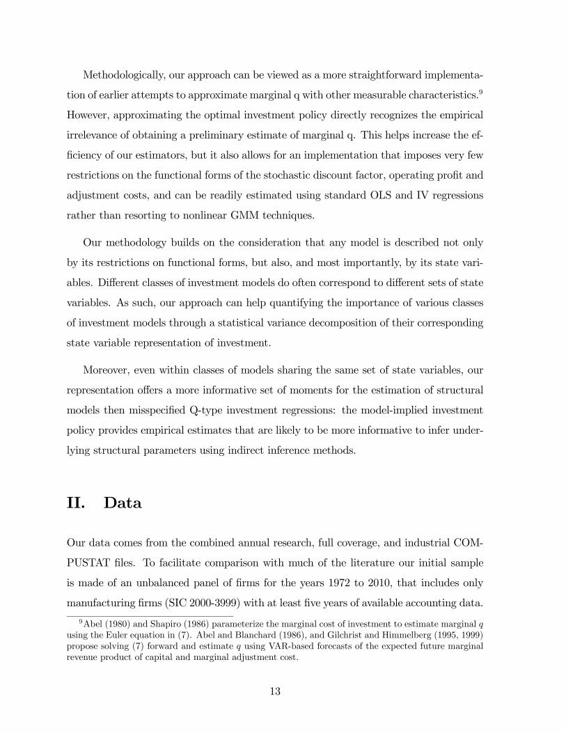
Methodologically, our approach can be viewed as a more straightforward implementa-

tion of earlier attempts to approximate marginal q with other measurable characteristics.9

However, approximating the optimal investment policy directly recognizes the empirical

irrelevance of obtaining a preliminary estimate of marginal q. This helps increase the ef-

ficiency of our estimators, but it also allows for an implementation that imposes very few

restrictions on the functional forms of the stochastic discount factor, operating profit and

adjustment costs, and can be readily estimated using standard OLS and IV regressions

rather than resorting to nonlinear GMM techniques.

Our methodology builds on the consideration that any model is described not only

by its restrictions on functional forms, but also, and most importantly, by its state vari-

ables. Different classes of investment models do often correspond to different sets of state

variables. As such, our approach can help quantifying the importance of various classes

of investment models through a statistical variance decomposition of their corresponding

state variable representation of investment.

Moreover, even within classes of models sharing the same set of state variables, our

representation offers a more informative set of moments for the estimation of structural

models then misspecified Q-type investment regressions: the model-implied investment

policy provides empirical estimates that are likely to be more informative to infer under-

lying structural parameters using indirect inference methods.

II. Data

Our data comes from the combined annual research, full coverage, and industrial COM-

PUSTAT files. To facilitate comparison with much of the literature our initial sample

is made of an unbalanced panel of firms for the years 1972 to 2010, that includes only

manufacturing firms (SIC 2000-3999) with at least five years of available accounting data.

9Abel (1980) and Shapiro (1986) parameterize the marginal cost of investment to estimate marginal qusing the Euler equation in (7). Abel and Blanchard (1986), and Gilchrist and Himmelberg (1995, 1999)propose solving (7) forward and estimate q using VAR-based forecasts of the expected future marginalrevenue product of capital and marginal adjustment cost.

13

Later, we also perform the analysis on a broader cross-section firms and using different

time periods.

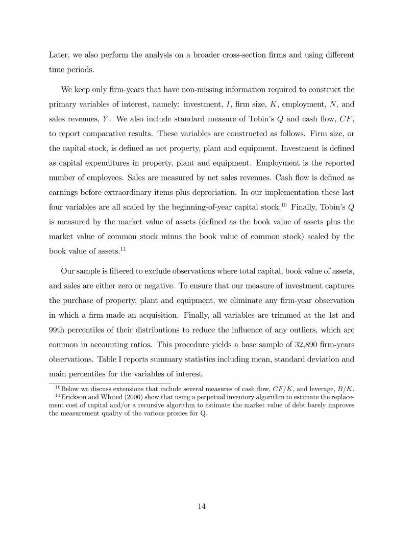
We keep only firm-years that have non-missing information required to construct the

primary variables of interest, namely: investment, I, firm size, K, employment, N , and

sales revenues, Y . We also include standard measure of Tobin’s Q and cash flow, CF ,

to report comparative results. These variables are constructed as follows. Firm size, or

the capital stock, is defined as net property, plant and equipment. Investment is defined

as capital expenditures in property, plant and equipment. Employment is the reported

number of employees. Sales are measured by net sales revenues. Cash flow is defined as

earnings before extraordinary items plus depreciation. In our implementation these last

four variables are all scaled by the beginning-of-year capital stock.10 Finally, Tobin’s Q

is measured by the market value of assets (defined as the book value of assets plus the

market value of common stock minus the book value of common stock) scaled by the

book value of assets.11

Our sample is filtered to exclude observations where total capital, book value of assets,

and sales are either zero or negative. To ensure that our measure of investment captures

the purchase of property, plant and equipment, we eliminate any firm-year observation

in which a firm made an acquisition. Finally, all variables are trimmed at the 1st and

99th percentiles of their distributions to reduce the influence of any outliers, which are

common in accounting ratios. This procedure yields a base sample of 32,890 firm-years

observations. Table I reports summary statistics including mean, standard deviation and

main percentiles for the variables of interest.

10Below we discuss extensions that include several measures of cash flow, CF/K, and leverage, B/K.11Erickson and Whited (2006) show that using a perpetual inventory algorithm to estimate the replace-

ment cost of capital and/or a recursive algorithm to estimate the market value of debt barely improvesthe measurement quality of the various proxies for Q.

14

III. Findings

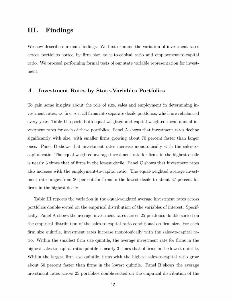
We now describe our main findings. We first examine the variation of investment rates

across portfolios sorted by firm size, sales-to-capital ratio and employment-to-capital

ratio. We proceed performing formal tests of our state variable representation for invest-

ment.

A. Investment Rates by State-Variables Portfolios

To gain some insights about the role of size, sales and employment in determining in-

vestment rates, we first sort all firms into separate decile portfolios, which are rebalanced

every year. Table II reports both equal-weighted and capital-weighted mean annual in-

vestment rates for each of these portfolios. Panel A shows that investment rates decline

significantly with size, with smaller firms growing about 70 percent faster than larger

ones. Panel B shows that investment rates increase monotonically with the sales-to-

capital ratio. The equal-weighted average investment rate for firms in the highest decile

is nearly 3 times that of firms in the lowest decile. Panel C shows that investment rates

also increase with the employment-to-capital ratio. The equal-weighted average invest-

ment rate ranges from 20 percent for firms in the lowest decile to about 37 percent for

firms in the highest decile.

Table III reports the variation in the equal-weighted average investment rates across

portfolios double-sorted on the empirical distribution of the variables of interest. Specif-

ically, Panel A shows the average investment rates across 25 portfolios double-sorted on

the empirical distribution of the sales-to-capital ratio conditional on firm size. For each

firm size quintile, investment rates increase monotonically with the sales-to-capital ra-

tio. Within the smallest firm size quintile, the average investment rate for firms in the

highest sales-to-capital ratio quintile is nearly 3 times that of firms in the lowest quintile.

Within the largest firm size quintile, firms with the highest sales-to-capital ratio grow

about 50 percent faster than firms in the lowest quintile. Panel B shows the average

investment rates across 25 portfolios double-sorted on the empirical distribution of the

15

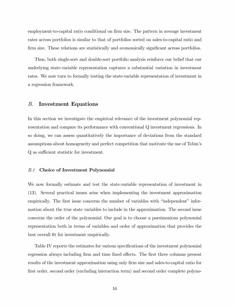
employment-to-capital ratio conditional on firm size. The pattern in average investment

rates across portfolios is similar to that of portfolios sorted on sales-to-capital ratio and

firm size. These relations are statistically and economically significant across portfolios.

Thus, both single-sort and double-sort portfolio analysis reinforce our belief that our

underlying state-variable representation captures a substantial variation in investment

rates. We now turn to formally testing the state-variable representation of investment in

a regression framework.

B. Investment Equations

In this section we investigate the empirical relevance of the investment polynomial rep-

resentation and compare its performance with conventional Q investment regressions. In

so doing, we can assess quantitatively the importance of deviations from the standard

assumptions about homogeneity and perfect competition that motivate the use of Tobin’s

Q as sufficient statistic for investment.

B.1 Choice of Investment Polynomial

We now formally estimate and test the state-variable representation of investment in

(13). Several practical issues arise when implementing the investment approximation

empirically. The first issue concerns the number of variables with “independent” infor-

mation about the true state variables to include in the approximation. The second issue

concerns the order of the polynomial. Our goal is to choose a parsimonious polynomial

representation both in terms of variables and order of approximation that provides the

best overall fit for investment empirically.

Table IV reports the estimates for various specifications of the investment polynomial

regression always including firm and time fixed effects. The first three columns present

results of the investment approximation using only firm size and sales-to-capital ratio for

first order, second order (excluding interaction term) and second order complete polyno-

16

mials, respectively. Including second order terms in firm size and sales-to-capital ratio,

except for the interaction term that is not statistically significant, increases the overall fit

for investment. The next three columns report instead the investment approximation us-

ing firm size, sales-to-capital ratio, and employment-to-capital ratio for first order, second

order (excluding interaction term) and second order complete polynomials, respectively.

First and second order terms in all variables are strongly statistically significant, ex-

cept for the second order term in the employment-to-capital ratio, which is significant

only at the 10 percent level. Interaction terms among the variables are generally not

statistically significant and do not improve much the quality of the approximation as

witnessed by the virtually unchanged adjusted R2. We omit higher order terms in the

polynomial representation because they are not statistically significant and are generally

not necessary to improve the quality of the approximation. Overall, while including sec-

ond order terms improves the approximation regardless of the variables selection, adding

the employment-to-capital ratio in the polynomial leaves instead virtually unaffected the

overall fit for investment. Hence, we focus on the second order polynomial approximation

in firm size and sales-to-capital ratio (column 2) as the best parsimonious state-variable

representation of investment empirically. We now provide comparisons with standard

Q-type regressions estimated using both fixed effect and first difference estimators.

B.2 Fixed Effect Estimators

We compare the empirical performance of the investment polynomial and standard Q

regressions. Table V reports the fixed effect (within-transformation) estimates for various

specifications of the investment regression always including firm and time fixed effects.

The first column presents results for the standard investment specification including only

Tobin’s Q. According to the neoclassical theory of investment (Hayashi, 1982; Abel and

Eberly, 1994), homogeneity of equal degree of a firm’s operating profit and investment cost

functions makes Tobin’s Q proportional to marginal q, and hence a sufficient statistic for

investment. The coefficient estimate on Tobin’s Q is positive and significant as predicted

by the neoclassical investment theory, but variation in Q can only account for 12 percent

17

of the within-variation in investment rates.

To account for potential nonlinearities in the relationship between investment and

Tobin’s Q, we add higher order terms in Q. As shown in the second column, includ-

ing a quadratic term in Q, while statistically significant, has only a negligible impact

on explanatory power with an adjusted R2 of about 13 percent. We omit for brevity

statistically insignificant higher order terms.

In the third column we report for easy of comparison our parsimonious state-variable

representation of investment including only linear and quadratic terms in firm size and

sales-to-capital ratio. Consistently with the convergence findings in Gala and Julio

(2011), firm size is negatively related to investment rates.12 The coefficient on the sales-

to-capital ratio - our proxy for productivity shocks - is positively related to investment as

predicted by the neoclassical theory of investment. The quadratic terms are also signifi-

cant and positively related to investment. The polynomial representation of investment

as function of the underlying state-variables spanned by firm size and sales-to-capital

ratio can account alone for up to 24 percent of the within-variation in investment rates.

Thus, our state-variable representation of investment outperforms by an order of mag-

nitude the conventional Q-investment regression (about 100 percent increase in adjusted

R2) implied by the standard homogeneous model.13

In the fourth and fifth columns, we add linear, and linear plus quadratic terms in Q

to our state-variable representation of investment, respectively. The inclusion of these

variables does not affect the significance of the polynomial representation of investment

and only leads to an increase in the adjusted R2 of about 15 percent starting from a value

of 24 percent up to 28 percent. Hence, Tobin’s Q, while not redundant, incorporates only

little valuable information for investment beyond the information already captured by

the measurable fundamental state variables. We further quantify the contribution of

12We obtain similar results, which we omit for brevity, when using past lags of capital stock either inplace of or as instrument for beginning-of-period capital stock. All results are available upon request.13Even when we follow the extant literature and arbitrarily add ad-hoc cash flow measures to the con-

ventional Q-investment regression, the overall explanatory power raises up only to 19 percent. As such,misspecified cash-flow augmented Q-investment regressions also underestimate (relative to our state-variable approximation) the overall empirical relevance of deviations from conventional homogeneityassumptions. All results are available upon request.

18

Tobin’s Q to the overall firm level investment variation in the next subsection.

B.3 First Difference Estimators

In Table VI we report the first-difference estimates for the same investment regressions

reported in Table V. The first difference specification mitigates concerns about the pres-

ence of serially correlated disturbance terms in empirical investment equations when run

in levels. When estimated in first-differences the overall significance of the state-variable

representation of investment is further reinforced. The polynomial representation of

investment as function of the underlying state-variables spanned by firm size and sales-

to-capital ratio can account alone for up to 30 percent of the variation in investment

rate changes. This is in sharp contrast with Q-investment regressions, which can only

account for up to 4 percent of the variation in investment rate changes. Hence, the gain

in adjusted R2 when using the state-variable representation of investment is even larger

in first-differences: about 7.8 times higher than the Q-investment specification. Further-

more, adding linear and/or quadratic terms in Q to our state-variable representation of

investment (specification 4 and 5) leaves virtually unchanged the overall significance and

explanatory power.

C. Variance Decomposition

To understand the relative importance of various variables in capturing investment vari-

ation we follow the analysis of covariance (ANCOVA) in Lemmon and Roberts (2008).

To do so we estimate the empirical model of investment:

Ijt+1Kjt

= βXjt + δj + ηt + εjt+1 (14)

where δj is a firm fixed effect and ηt is a year fixed effect. X denotes a vector of

explanatory variables that includes various combinations of Tobin’s Q, cash flow, and

the state-variable polynomial in firm size, lnK, and sales-to-capital ratio, lnY/K.

19

Table VII reports the results of this covariance decomposition for several specifica-

tions. Each column in the table corresponds to a different specification for investment.

The numbers reported in the table, excluding the adjusted R2 reported in the last row,

correspond to the fraction of the total Type III partial sum of squares for a particular

model.14 That is, we normalize the partial sum of squares for each effect by the aggre-

gate partial sum of squares across all effects in the model, so that each column sums to

one. Intuitively, each value in the table corresponds to the fraction of the model sum of

squares attributable to a particular effect (i.e. firm, year, Q, cash flow, etc.). Panel A

of Table VII provides estimates based on fixed effect estimators, while Panel B reports

estimates based on first difference estimators.

As shown in Panel A, column 1, firm and year fixed effects capture 28 percent of

the variation in investment rates, of which 84 percent can be attributable to firm fixed

effects alone. As discussed above, firm fixed effects capture cross sectional variation in

the depreciation rate, δj, which is equal to the long run or steady-state investment rate.

As such, we should expect firm fixed effects to account for a large variation in investment

rates.15 Moreover, unlike studies on the empirical determinants of leverage, for exam-

ple, these fixed effects have strong economic (as opposed to purely statistical) content

supporting their empirical significance. Year fixed effects, which capture unobserved ag-

gregate variation, account instead for, at most, only 16 percent of the total explained

variation in investment.

Augmenting the firm and time fixed effects specification with Tobin’s Q increases the

total adjusted R2 for investment from 28 percent to 33 percent. However, only 8 percent

of the explained sum of squares captured by the included covariates can be attributed to

Tobin’s Q.

Column 3 shows the variance decomposition associated with the state-variable poly-

nomial, including only fixed effects. To highlight the significant incremental contribution

14We use Type III sum of squares because (i) the sum of squares is not sensitive to the ordering ofthe covariates, and (ii) our data is unbalanced (some firms have more observations than others).15In fact, most investment models predict that in the long run all cross-sectional variation in investment

is captured by δj alone.

20

of the state-variable representation in accounting for variation in investment, we notice

that the adjusted R2 increases from 28 percent to 42 percent. About 1/4 of this overall

variation can now be attributed to the state-variable polynomial. And in fact, adding

Tobin’s Q to our core state variables only increases the adjusted R2 marginally from

42 percent to 45 percent. Most importantly, only 7 percent of the overall variation can

now be attributed to Tobin’s Q, while 32 percent is attributable to the state-variable

polynomial. Overall, our parsimonious state-variable polynomial accounts for more than

four times as much as Tobin’s Q of the total explained variation in investment.

The variance decomposition of investment rates changes in Panel B contributes to

strengthen the previous results. Year fixed effects alone can only capture about 1 percent

of the variation in investment rate changes. Augmenting the time fixed effects specifi-

cation with Tobin’s Q increases the adjusted R2 for investment changes only marginally

from 1 to 4 percent.

Instead, our state-variable polynomial including only fixed effects accounts for up to 30

percent of the total variation in investment changes, of which 98 percent are attributable

to the state-variable polynomial alone. Adding Tobin’s Q to our core state variables

only marginally increases the adjusted R2 to 31 percent. Most importantly, Tobin’s Q

accounts only for 2 percent of the overall explained variation in investment changes,

which is as much as year fixed effects, while 96 percent is attributable to our core state

variables. Overall, Tobin’s Q incorporates only very little “independent” information for

investment beyond the information already captured by our fundamental state variables.

D. Alternative Samples

Capital-intensive manufacturing firms form probably the most reliable panel for this

study, but it is nevertheless interesting to examine how both approaches would perform

on different samples. Table VIII reports the results for three alternative panels. The

first column looks at a panel that now includes all firms except those in the financial

sector, regulated utilities and public services. The second shows the results for a panel

21

covering only the period between 1982-2010, which many authors focus on.16 The third

column reports the results for a balanced panel of manufacturing firms during the period

1982-2010.

Adding non-manufacturing firms substantially expands the sample and the statistical

significance of our estimates, but it does not affect the overall goodness of fit. On the other

hand, eliminating the first ten years of data from our baseline sample slightly improves

overall performance. The main results are also confirmed on the smaller balanced sample,

which shows that our findings are not driven by the attrition in database due to firms’

entry and exit.

IV. Extensions

In this section we extend the basic methodology to address the impact on investment of (i)

unobserved aggregate state variables entering the investment equation in a non-additive

fashion; (ii) firm-specific shocks to the price of variable inputs of production such as

wages; (iii) financial market frictions; and (iv) alternative adjustment cost specifications

such as those proposed in Eberly, Rebelo and Vincent (2011).

A. Aggregate Shocks and Time-Specific Coefficients

A complete state-variable representation of investment in (11) would also include the

aggregate state variables, Ω, as part of the exogenous state Z. The set of aggregate state

variables affecting investment may include, among others, aggregate shocks to produc-

tivity, wages, capital adjustment costs, relative price of investment goods, and represen-

tative household preferences. While the measurement of our firm level state variables,

like sales and size, already captures part of the variation in these underlying aggregate

state variables, there may still be substantial investment variation attributable to omit-

16Several different subsamples were also examined without noticeable changes in the findings. Allresults are available upon request.

22

ted variation in these aggregate state variables. For instance, part of the variation in

aggregate productivity shocks would be captured by our measure of firm level produc-

tivity, however, aggregate productivity shocks may still affect firm investment indirectly

through the stochastic discount factor, M , by affecting risk premia.

Given a large panel of firms, the complete knowledge of the aggregate state variables

in Ω is not necessary for the purpose of estimating investment. In fact, we can capture

the impact of all unobserved aggregate variation, above and beyond the variation already

incorporated in the measured firm level state variables, by allowing not only for time fixed

effects, but also for time-specific polynomial slope coefficients. While introducing time

fixed effects in the approximate investment equation captures unobserved aggregate vari-

ation that affects all firms equally, including time-varying polynomial slope coefficients

also accounts for unobserved variation in the aggregate state variables that affects firms

differently.

More precisely, allowing for time-specific polynomial coefficients in our baseline firm

level state variables, k and y, is equivalent to a tensor product polynomial representation

of investment which includes a complete set of time dummies, η, as state variables:

Ijt+1Kjt

'nkXik=0

nyXiy=0

nηXiη=0

bik,iy,iη × kikjt × yiyjt × η

iηt =

nkXik=0

nyXiy=0

dik,iy,t × kikjt × yiyjt (15)

where the equality follows from the fact that ηiηt = ηt for any iη ≥ 0, and dik,iy,t ≡

ηt ×Pnη

iη=0bik,iy,iη . Given the correct set of firm level state variables, allowing for time-

specific polynomial coefficients fully captures all relevant unobserved variation in aggre-

gate economic conditions.

We implement empirically the baseline polynomial approximation with time-specific

coefficients including firm fixed effects. Table IX reports the estimates of the average

partial effects for each firm-level state variable in the polynomial approximation. The

first column provides estimates based on the benchmark unbalanced panel of manufac-

turing firms for the period 1972-2010. The average coefficients are in line with previous

estimates for the same polynomial without time-specific slopes as reported in column

23

(4) of Table V. The baseline firm level state variables, namely sales and size, are on

average significant, except for the second order term in firm size. The introduction of

time-specific slopes, while allowing for a more flexible investment specification, trades off

efficiency for goodness-of-fit. Figure 1 plots the time-specific coefficients on each of the

polynomial terms along with the corresponding 95 percent confidence intervals. Slope

coefficients exhibit substantial variation over time, with estimates preserving their sign

over the sample period, except for few, mainly statistically insignificant, exceptions. The

efficiency loss in the estimation of the time-specific polynomial is compensated, however,

only with a marginal improvement in the overall fit for investment. Even though allowing

for time-specific coefficients increases only marginally the total explained sum of squares

(R2 moves from 42 percent to 43 percent only), the fraction attributable to the state

variable polynomial representation increases from 25 percent up to 37 percent as shown

by the variance decomposition in Table XIII (column 2).

The different size of each cross section may affect the efficiency and the overall

goodness-of-fit for our previous estimates, which are based on the unbalanced panel.

For comparison, we provide the time-specific estimates based on the balanced panel of

manufacturing firms for the period 1982-2010 in the second column of Table IX and Fig-

ure 2. The average coefficients in Table IX are consistent both in terms of magnitude and

significance with previous estimates for the same polynomial without time-specific slopes

as reported in column (3) of Table VIII. As shown in Figure 2, the slope coefficients

exhibit substantial time variation also in the balanced sample. The point estimates tend

to consistently preserve their sign over time, with very few exceptions. Differently from

the unbalanced panel, the added flexibility of the time-varying polynomial produces now

an overall better fit for investment.

B. Labor Market Shocks and Cash Flow Data

The use of employment data in equation (13) raises two issues. The first is practical.

Data on employment is relatively sparse in Compustat and data on hours is simply

24

not available. The second concern is theoretical. If firm-specific wage shocks are very

important, then Z 6= A and equation (13) can actually be misspecified.17

Although we think this is unlikely for most firms, the profit maximizing equation (1)

does offer one possible way to address this concern. Whenever the labor share is constant,

we can use the definition of operating profits in (1) and construct the unobserved state

variable z instead from

z = π − θKk (16)

where π = logΠ, and z now captures both the productivity/demand, A, and wage

shock, W , and θK is the share of capital in operating profit. In this case, the empirical

investment equation can be rewritten as:

I

K'

nkXik=0

nπXiπ=0

aik,iπkikπiπ (17)

which now can be implemented using data on operating profits and stock of capital.

Imposing a constant labor share, however, restricts the production function to be Cobb-

Douglas, which is generally not at odds with the empirical evidence.18

Table X implements our polynomial approximation using several alternative measures

of cash flows. The first column reports the results of estimating equation (17) using the

classic measure of cash flow (earnings before extraordinary items plus depreciation). The

next two columns are estimated using measures constructed from the uses and sources

of funds. In the second column, we adjust operating income for investments in working

capital and, more significantly, for non-recurring charges as in Lewellen and Lewellen

(2011). Estimates in the third column use a measure that further adds interest and

related expense and subtracts nonoperating income (expense). The main downside about

using these measures of cash flow is the reduced sample size, given that data on sources

17Recall that time and industry fixed effects will capture any other variation in wages and indeed inthe price of any other variable input of production.18Let F (K,N) = KαKNαN . Profit maximization implies that, Π (K,Z) = ZKθK , where θK =

αK/ (1− αN ), and Z = (1− αN ) [A (αN/W )αN ]

11−αN . This includes shocks to productivity, output

demand, as well as variations in factor prices.

25

and uses of funds are not always readily available. However, at least in our specifications,

this does not have any noticeable impact on the results. The final column in the table

returns to the more widely available income statement data, which defines cash flow as

simply operating income plus depreciation expenses.

Although there are some differences across the various measures of cash flows, point

estimates, levels of significance and goodness of fit are all substantively comparable.

Overall, we find that these specifications perform slightly less well than the baseline

specification which includes firm sales instead of cash flow. However, the variance de-

composition in Table XIII (column 3) shows that, even though using cash flow instead

of sales reduces the total explained sum of squares (R2 moves from 42 percent to 40

percent), about 35 percent of it can be attributed to the covariation with the polynomial

in cash flow and size alone.

C. Capital Market Imperfections and Leverage

For clarity of exposition, our structural model in Section I. purposely avoids any discus-

sion of financial market imperfections and assumes that the Modigliani-Miller theorem

holds. An important benefit of this simplified environment is that it demonstrates very

clearly how we can generate cash flow and size effects purely as result of adopting more

realistic technologies (as in Gomes, 2001; and Abel and Eberly, 2010, for example).

Since our approach does not rely on the estimation of marginal q, it can naturally

accommodate modern models where marginal q is no longer a sufficient statistics for

investment, such as models with financial frictions, by allowing for the presence of addi-

tional state variables in the optimal investment policy, G (·).

While an exhaustive analysis of the impact of financial market imperfections on in-

vestment is beyond the scope of this paper, it is well known that most modifications of

the firm problem in (4), that allow for such plausible frictions as tax benefits of debt,

collateral requirements and costly external financing, often imply that debt, B, becomes

26

an additional state variable for the optimal investment policy, so that:19

I/K = G (K,B,Z) . (18)

It follows that we can generalize our procedure to derive empirical investment equations

that now include leverage terms as additional state variables.20

Table XI shows the results of introducing leverage to our baseline state variable ap-

proximation of investment. Like our measure of cash flow, there are several measures of

the (book) leverage ratio. In Table XI, we only report results for the two most widely used

measures of leverage.21 The first column measures debt as the sum of short-term plus

long-term debt, while the second column uses a measure of net leverage, by subtracting

cash and short-term investments from debt.

Our estimates show that all leverage terms are generally statistically significant con-

firming that there is indeed some degree of interaction between financing and investment

decisions of firms. The negative point estimates are also generally consistent with theo-

retical restrictions imposed by most models of financing frictions.

The variance decomposition in Table XIII, however, raises some concerns about the

quantitative importance of leverage for the investment decisions of this broad cross-

section of firms. A Type III variance decomposition for the state variables approximation

including net leverage (column 4) shows that only 3 percent of the explained sum of

squares can be captured by the covariation with firm leverage.

It is surely premature to conclude from this that financial market imperfections are not

particularly important in determining capital expenditures. Leverage may be of greater

importance for some specific subsets of firms or different formulations of the structural

19Examples of such models with capital market imperfections where net financial liabilities representsan additional state variable for the optimal investment policy include Whited (1992), Bond and Meghir(1994), Gilchrist and Himmelberg (1999), Hennessy, Levy, and Whited (2007), Bustamante (2011), andBolton, Chen, and Wang (2012), among others.20Without loss of generality, we normalize debt by the stock of capital and use B/K in the empirical

analysis.21Using several alternative measures of leverage does not alter the main findings. These results are

available upon request.

27

model may lead to more precise restrictions on the form of investment equations. While

we leave these possibilities for future work, it is immediate to see how they can be readily

accommodated in our structured approach.22

D. Alternative Adjustment Costs and Lagged Investment

Our investigation of the role of leverage can be further expanded to discuss the issue

of econometric specification more broadly. Time-to-build, non-smooth adjustment costs,

and even labor market distortions, can all lead to more complex forms of investment

equation (10).

Notably, Eberly, Rebelo and Vincent (2011) provide some evidence that lagged in-

vestment is empirically the most significant determinant of contemporaneous investment,

and attribute this to more elaborate adjustment cost functions, Φ (·), such as those pro-

posed in Christiano, Eichenbaum, and Evans (2005).23 Alternatively, building lags offer

also an explanation to the documented serial correlation in investment expenditures and

a possible micro foundation for more complex adjustment costs.24

Our approach can naturally accommodate such frictions as time-to-build and more

complex adjustment cost specifications like in Eberly, Rebelo and Vincent (2011), by

including lagged investment as additional state variable in the optimal investment policy,

G (·).

We investigate the role of lagged investment in Tables XII and XIII. To address

22Gala and Gomes (2012) explore the implications of several alternative financing constraints on theempirical investment equation and estimate it on various sub-panels.23Eberly, Rebelo and Vincent (2011) specify capital adjustment costs in the capital accumulation

equation, and assume a formulation that depends on the growth rate of investment. Specifically, theyuse the following linear-quadratic adjustment cost function:

Φ (It, It−1) =

"1− ξ

µItIt−1

− γ

¶2#It

where ξ controls the size of the adjustment cost and γ denotes the firm steady-state growth rate. Thisadjustment cost specification makes lagged investment, It−1, a relevant state variable for the firm optimalinvestment policy.24Of course the lagged investment effect can also reflect the presence of more complicated, i.e. non-

Markov, exogenous shocks.

28

endogeneity issues in dynamic panel data with a lagged dependent variable, we instru-

ment lagged investment with prior two lags of its first-difference. Table XII provides

the results of several investment specifications including lagged investment. We report

for comparison the investment specification in Eberly, Rebelo and Vincent (2011), which

includes lagged investment and cash flow to a conventional Q-type regression. Consistent

with the evidence in Eberly, Rebelo and Vincent (2011), lagged investment enters with

a positive and significant coefficient, and increases the overall fit to investment. Table

XII also reports the estimates of our baseline state variable approximation augmented

with lagged investment. While lagged investment enters significantly, its inclusion affects

neither the point estimates nor the significance of our baseline state variable approxima-

tion, and only increases the total adjusted R2 from 42 percent to 46 percent. Table XIII

provides its variance decomposition (column 5). Even though lagged investment remains

an important determinant, its share of the total explained variation in investment is less

than one third of that accounted by our core state variables, which still capture a large

fraction of the explained variation in investment.25

V. Conclusion

This paper questions the widespread use of Q-ratios in empirical work. Instead, we

propose an asset price-free alternative relying on the insight that the optimal investment

policy is a function of much more easily measurable state variables. Under very general

assumptions about the nature of technology and markets, our approach ties investment

rates directly to firm size and either sales or cash flows, even in the absence of financial

market frictions. Our methodology can also account for capital markets imperfections

by augmenting the set of measurable state variables with observable leverage. Similarly,

it can accommodate such frictions as time-to-build and more complex adjustment cost

specifications like in Eberly, Rebelo and Vincent (2011), by including lagged investment

as additional state variable for the optimal investment policy. Furthermore, our approach

25These results are virtually unchanged when leverage is included to the state variable approximationof investment.

29

can easily account for the impact of aggregate variation, above and beyond the variation

already incorporated in the measured firm level state variables, by augmenting the set

of state variables in the polynomial approximation with time dummies. We show that

the empirical performance of our methodology is noticeably superior to that of standard

Q-based investment equations.

Are measures of Tobin’s Q at all informative? Measures of Tobin’s Q may still contain

valuable information beyond the information identifiable through measurable state vari-

ables. As such, whenever measurement error in market values does not represent a major

concern, we can always use Tobin’s Q as a useful catch-all variable to account for omitted

state variables rather than as primary determinant of investment. Indeed, using Tobin’s

Q as “residual” variable in investment regressions may capture relevant variation in un-

observed firm-specific time-varying state variables including, for instance, firm-specific

persistent shocks to input adjustment costs. However, the empirical evidence suggests

otherwise.

30

References

Abel, AndrewB., “Empirical Investment Equations: An Integrative Framework”, Carnegie-

Rochester Conferences on Economic Policy, 12, 29-91, 1980.

Abel, Andrew B. and Olivier Blanchard, “The Present Value of Profits and Cyclical

Movements in Investments”, Econometrica, 54, 249-273, 1986.

Abel, Andrew B. and Janice Eberly, “A Unified Model of Investment Under Uncer-

tainty”, American Economic Review, 84, 1369-1384, 1994.

Abel, Andrew B. and Janice Eberly, “An Exact Soultion for the Investment and Market

Value of a Firm Facing Uncertainty, Adjustment Costs, and Irreversibility”, Journal

of Economic Dynamics and Control 21, 831-852, 1997.

Abel, Andrew B. and Janice Eberly, “Investment and q with Fixed Costs: An Empirical

Investigation”, unpublished manuscript, University of Pennsylvania, 2002.

Asker, J., J. Farre-Mensa, and A. Ljungqvist, “Comparing the Investment Behavior of

Public and Private Firms”, Working Paper, 2011.

Blanchard, Olivier, Changyong Rhee, and Lawrence Summers, “The Stock Market,

Profit and Investment”, Quarterly Journal of Economics, 108, 261-288, 1993.

Bolton Patrick, Hui Chen, and Neng Wang, “A Unified Theory of Tobin’s q, Corporate

Investment, Financing, and Risk Management”, Journal of Finance, forthcoming,

2012.

Bond, Stephen and Costas Meghir, “Dynamic Investment Models and the Firms’ Fi-

nancial Policy”, Review of Economic Studies 61, 197-222, 1994.

Bustamante, Maria Cecilia, “How do Frictions affect Corporate Investment? A struc-

tural approach”, Working Paper, 2011.

Caballero, Ricardo and John Leahy, “Fixed Costs and the Demise of Marginal q”, NBER

Working Paper #5508, 1996.

Christiano, Lawrence, Martin Eichenbaum, and Charles Evans, “Nominal Rigidities and

the Dynamic Effect of a Shock to Monetary Policy,” Journal of Political Economy,

113, 1-45, 2005.

31

Cooper, Russell and João Ejarque, “Financial Frictions and Investment: A Requiem in

Q”, Review of Economic Dynamics, 6, 710—728, 2003.

Cooper, Russell and John Haltiwanger, “On the nature of capital adjustment costs”,

Review of Economic Studies 73, 611-633, 2006.

Eberly, Janice, Sergio Rebelo, and Nicolas Vincent, “What Explains the Lagged Invest-

ment Effect?”, Journal of Monetary Economics, forthcoming, 2011.

Erickson, Timothy and Toni Whited, “Measurement Error and the Relationship Be-

tween Investment and q”, Journal of Political Economy, 108, 1027-57, 2000.

Erickson, Timothy and Toni Whited, “On the Accuracy of Different Measures of Q”,

Financial Management, 35, 5-33, 2006.

Erickson, Timothy and Toni Whited, “Treating Measurement Error in Tobin’s q”, Re-

view of Financial Studies, forthcoming, 2011.

Fazzari, Steven M., Hubbard, R. Glenn, and Petersen, Bruce C., “Financing Constraints

and Corporate Investment”, Brookings Papers Economic Activity, 1, 141-95, 1988.

Gala, Vito D. and Brandon Julio, “Convergence in Corporate Investments”, Working

Paper, London Business School, 2011.

Gala, Vito D. and João F. Gomes, “Estimating Investment with Financing Frictions”,

working paper, The Wharton School, 2012.

Gilchrist, Simon and Charles Himmelberg, “Evidence on the Role of Cash Flow in

Investment”, Journal of Monetary Economics, 36, 541-572, 1995.

Gilchrist, Simon and Charles Himmelberg, 1998, “Investment: Fundamentals and Fi-

nance”, in NBER Macroeconommics Annual, Ben Bernanke and Julio Rotemberg

eds, MIT Press

Gomes, João F., “Financing Investment”, American Economic Review, 90, 5, 1263-1285,

2001.

Hayashi, Fumio, “Tobin’s Marginal and Average q: A Neoclassical Interpretation”,

Econometrica, 50, 213-224, 1982.

Hennessy, Christopher and Toni Whited, “How Costly is External Financing? Evidence

from a Structural Estimation”, Journal of Finance, 62, 1705-1745, 2007.

32

Hennessy, Christopher, Amnon Levy and Toni Whited, “Testing Q theory with financing

frictions”, Journal of Financial Economics, 83, 691-717, 2007.

Hubbard, R. Glenn., “Capital-Market Imperfections and Investment”, Journal of Eco-

nomic Literature, 36, 193-225, 1998.

Hubbard, R. Glenn, Anil Kashyap and Toni Whited, “Internal Finance and Firm In-

vestment”, Journal of Money, Credit and Banking, 27, 683-701, 1995.

Jorgenson, Dale W., “Capital Theory and Investment Behavior”, American Economic

Review, 33, 247-259, 1963.

Philippon, Thomas, “The Bond Market’s Q”, Quarterly Journal of Economics, 124 (3),

1011-1056, 2009.

Shapiro, Matthew, “The Dynamic Demand for Capital and Labor”, Quarterly Journal

of Economics 101, 513-542, 1986.

Tobin, James, “A General Equilibrium Approach to Monetary Theory”, Journal of

Money Credit and Banking, 1, 15-29, 1969.

Whited, Tony, “Debt, Liquidity Constraints, and Corporate Investment: Evidence from

Panel Data”, Journal of Finance 47, 1425-1460, 1992.

33

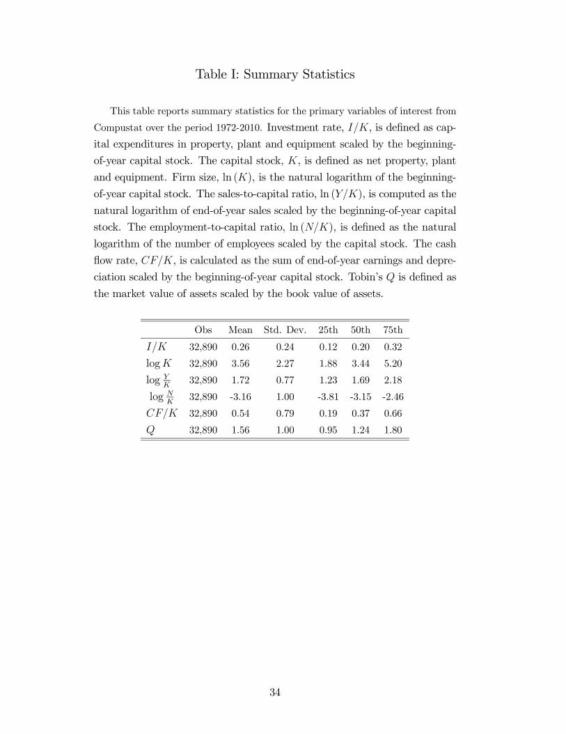
Table I: Summary Statistics

This table reports summary statistics for the primary variables of interest from

Compustat over the period 1972-2010. Investment rate, I/K, is defined as cap-

ital expenditures in property, plant and equipment scaled by the beginning-

of-year capital stock. The capital stock, K, is defined as net property, plant

and equipment. Firm size, ln (K), is the natural logarithm of the beginning-

of-year capital stock. The sales-to-capital ratio, ln (Y/K), is computed as the

natural logarithm of end-of-year sales scaled by the beginning-of-year capital

stock. The employment-to-capital ratio, ln (N/K), is defined as the natural

logarithm of the number of employees scaled by the capital stock. The cash

flow rate, CF/K, is calculated as the sum of end-of-year earnings and depre-

ciation scaled by the beginning-of-year capital stock. Tobin’s Q is defined as

the market value of assets scaled by the book value of assets.

Obs Mean Std. Dev. 25th 50th 75th

I/K 32,890 0.26 0.24 0.12 0.20 0.32

logK 32,890 3.56 2.27 1.88 3.44 5.20

log YK

32,890 1.72 0.77 1.23 1.69 2.18

log NK

32,890 -3.16 1.00 -3.81 -3.15 -2.46

CF/K 32,890 0.54 0.79 0.19 0.37 0.66

Q 32,890 1.56 1.00 0.95 1.24 1.80

34

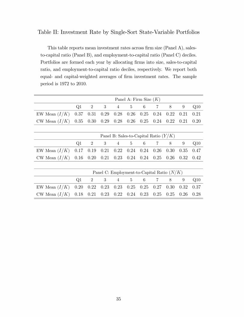
Table II: Investment Rate by Single-Sort State-Variable Portfolios

This table reports mean investment rates across firm size (Panel A), sales-

to-capital ratio (Panel B), and employment-to-capital ratio (Panel C) deciles.

Portfolios are formed each year by allocating firms into size, sales-to-capital

ratio, and employment-to-capital ratio deciles, respectively. We report both

equal- and capital-weighted averages of firm investment rates. The sample

period is 1972 to 2010.

Panel A: Firm Size (K)

Q1 2 3 4 5 6 7 8 9 Q10

EW Mean (I/K) 0.37 0.31 0.29 0.28 0.26 0.25 0.24 0.22 0.21 0.21

CW Mean (I/K) 0.35 0.30 0.29 0.28 0.26 0.25 0.24 0.22 0.21 0.20

Panel B: Sales-to-Capital Ratio (Y/K)

Q1 2 3 4 5 6 7 8 9 Q10

EW Mean (I/K) 0.17 0.19 0.21 0.22 0.24 0.24 0.26 0.30 0.35 0.47

CW Mean (I/K) 0.16 0.20 0.21 0.23 0.24 0.24 0.25 0.26 0.32 0.42

Panel C: Employment-to-Capital Ratio (N/K)

Q1 2 3 4 5 6 7 8 9 Q10

EW Mean (I/K) 0.20 0.22 0.23 0.23 0.25 0.25 0.27 0.30 0.32 0.37

CW Mean (I/K) 0.18 0.21 0.23 0.22 0.24 0.23 0.25 0.25 0.26 0.28

35

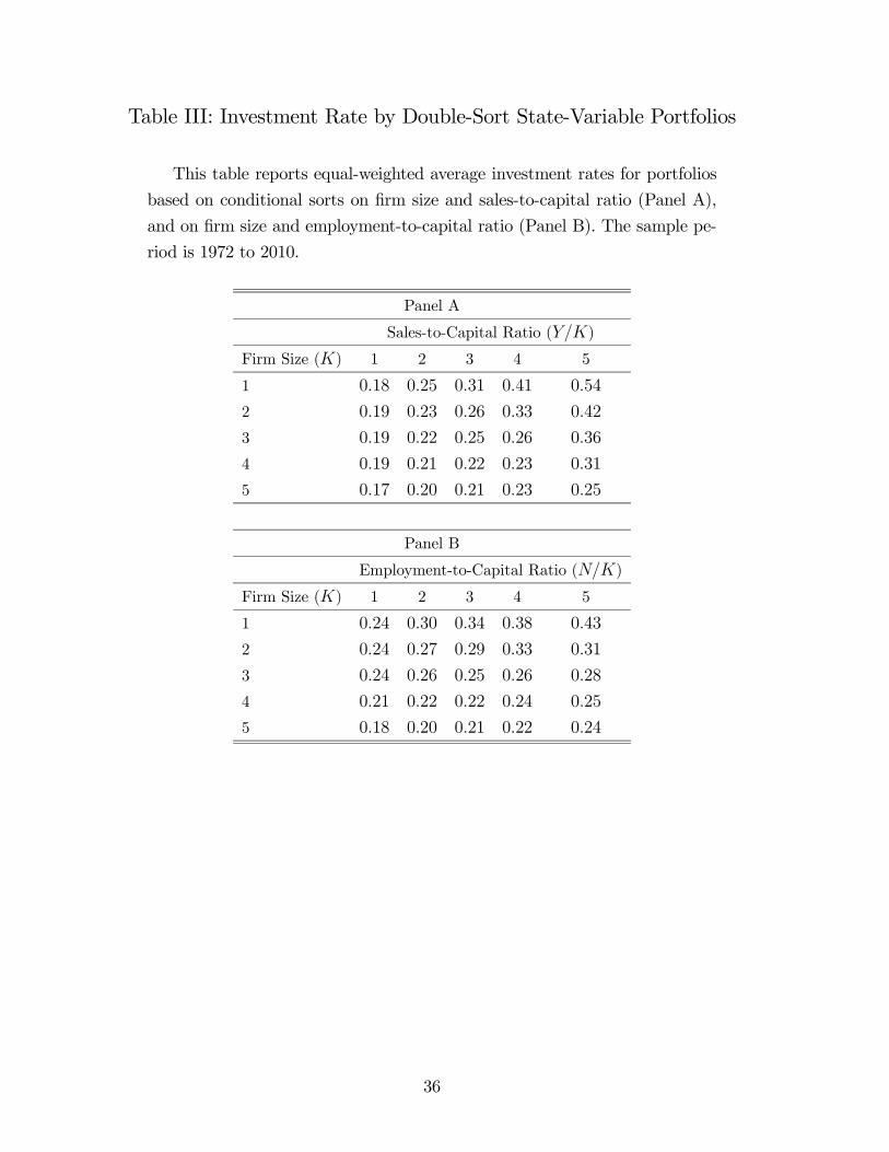
Table III: Investment Rate by Double-Sort State-Variable Portfolios

This table reports equal-weighted average investment rates for portfolios

based on conditional sorts on firm size and sales-to-capital ratio (Panel A),

and on firm size and employment-to-capital ratio (Panel B). The sample pe-

riod is 1972 to 2010.

Panel A

Sales-to-Capital Ratio (Y/K)

Firm Size (K) 1 2 3 4 5

1 0.18 0.25 0.31 0.41 0.54

2 0.19 0.23 0.26 0.33 0.42

3 0.19 0.22 0.25 0.26 0.36

4 0.19 0.21 0.22 0.23 0.31

5 0.17 0.20 0.21 0.23 0.25

Panel B

Employment-to-Capital Ratio (N/K)

Firm Size (K) 1 2 3 4 5

1 0.24 0.30 0.34 0.38 0.43

2 0.24 0.27 0.29 0.33 0.31

3 0.24 0.26 0.25 0.26 0.28

4 0.21 0.22 0.22 0.24 0.25

5 0.18 0.20 0.21 0.22 0.24

36

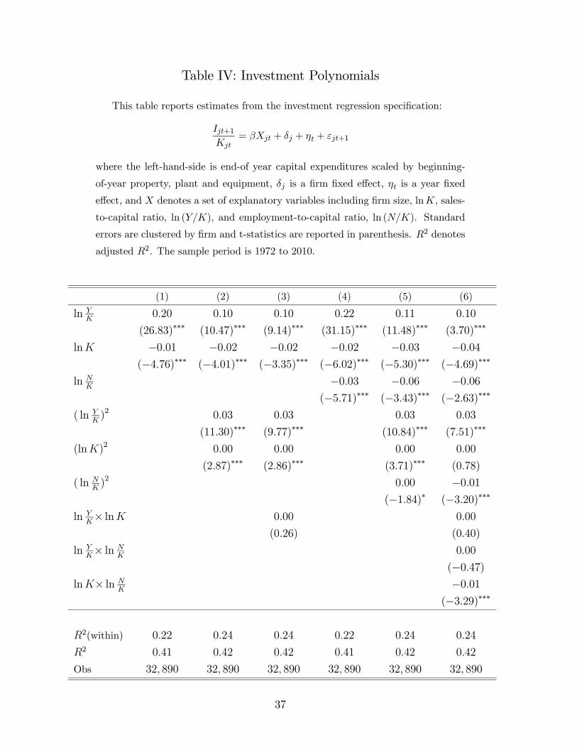
Table IV: Investment Polynomials

This table reports estimates from the investment regression specification:

Ijt+1Kjt

= βXjt + δj + ηt + εjt+1

where the left-hand-side is end-of year capital expenditures scaled by beginning-

of-year property, plant and equipment, δj is a firm fixed effect, ηt is a year fixed

effect, and X denotes a set of explanatory variables including firm size, lnK, sales-

to-capital ratio, ln (Y/K), and employment-to-capital ratio, ln (N/K). Standard

errors are clustered by firm and t-statistics are reported in parenthesis. R2 denotes

adjusted R2. The sample period is 1972 to 2010.

(1) (2) (3) (4) (5) (6)

ln YK

0.20 0.10 0.10 0.22 0.11 0.10

(26.83)∗∗∗ (10.47)∗∗∗ (9.14)∗∗∗ (31.15)∗∗∗ (11.48)∗∗∗ (3.70)∗∗∗

lnK −0.01 −0.02 −0.02 −0.02 −0.03 −0.04(−4.76)∗∗∗ (−4.01)∗∗∗ (−3.35)∗∗∗ (−6.02)∗∗∗ (−5.30)∗∗∗ (−4.69)∗∗∗

ln NK

−0.03 −0.06 −0.06(−5.71)∗∗∗ (−3.43)∗∗∗ (−2.63)∗∗∗

( ln YK)2 0.03 0.03 0.03 0.03

(11.30)∗∗∗ (9.77)∗∗∗ (10.84)∗∗∗ (7.51)∗∗∗

(lnK)2 0.00 0.00 0.00 0.00

(2.87)∗∗∗ (2.86)∗∗∗ (3.71)∗∗∗ (0.78)

( ln NK)2 0.00 −0.01

(−1.84)∗ (−3.20)∗∗∗

ln YK× lnK 0.00 0.00

(0.26) (0.40)

ln YK× ln N

K0.00

(−0.47)lnK× ln N

K−0.01

(−3.29)∗∗∗

R2(within) 0.22 0.24 0.24 0.22 0.24 0.24

R2 0.41 0.42 0.42 0.41 0.42 0.42

Obs 32, 890 32, 890 32, 890 32, 890 32, 890 32, 890

37

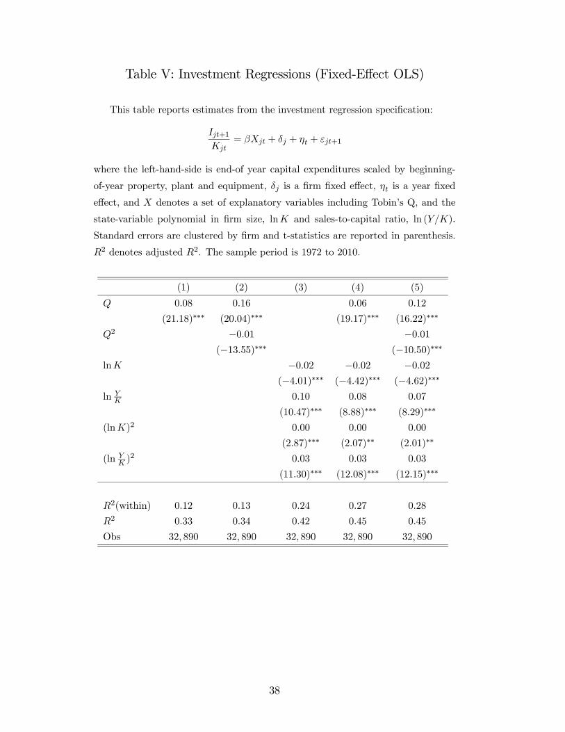
Table V: Investment Regressions (Fixed-Effect OLS)

This table reports estimates from the investment regression specification:

Ijt+1Kjt

= βXjt + δj + ηt + εjt+1

where the left-hand-side is end-of year capital expenditures scaled by beginning-

of-year property, plant and equipment, δj is a firm fixed effect, ηt is a year fixed

effect, and X denotes a set of explanatory variables including Tobin’s Q, and the

state-variable polynomial in firm size, lnK and sales-to-capital ratio, ln (Y/K).

Standard errors are clustered by firm and t-statistics are reported in parenthesis.

R2 denotes adjusted R2. The sample period is 1972 to 2010.

(1) (2) (3) (4) (5)

Q 0.08 0.16 0.06 0.12

(21.18)∗∗∗ (20.04)∗∗∗ (19.17)∗∗∗ (16.22)∗∗∗

Q2 −0.01 −0.01(−13.55)∗∗∗ (−10.50)∗∗∗

lnK −0.02 −0.02 −0.02(−4.01)∗∗∗ (−4.42)∗∗∗ (−4.62)∗∗∗

ln YK 0.10 0.08 0.07

(10.47)∗∗∗ (8.88)∗∗∗ (8.29)∗∗∗

(lnK)2 0.00 0.00 0.00

(2.87)∗∗∗ (2.07)∗∗ (2.01)∗∗

(ln YK )

2 0.03 0.03 0.03

(11.30)∗∗∗ (12.08)∗∗∗ (12.15)∗∗∗

R2(within) 0.12 0.13 0.24 0.27 0.28

R2 0.33 0.34 0.42 0.45 0.45

Obs 32, 890 32, 890 32, 890 32, 890 32, 890

38

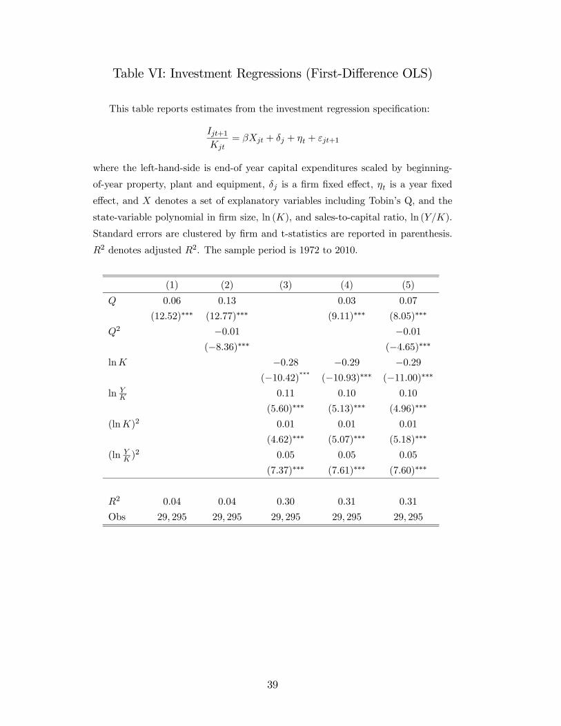
Table VI: Investment Regressions (First-Difference OLS)

This table reports estimates from the investment regression specification:

Ijt+1Kjt

= βXjt + δj + ηt + εjt+1

where the left-hand-side is end-of year capital expenditures scaled by beginning-

of-year property, plant and equipment, δj is a firm fixed effect, ηt is a year fixed

effect, and X denotes a set of explanatory variables including Tobin’s Q, and the

state-variable polynomial in firm size, ln (K), and sales-to-capital ratio, ln (Y/K).

Standard errors are clustered by firm and t-statistics are reported in parenthesis.

R2 denotes adjusted R2. The sample period is 1972 to 2010.

(1) (2) (3) (4) (5)

Q 0.06 0.13 0.03 0.07

(12.52)∗∗∗ (12.77)∗∗∗ (9.11)∗∗∗ (8.05)∗∗∗

Q2 −0.01 −0.01(−8.36)∗∗∗ (−4.65)∗∗∗

lnK −0.28 −0.29 −0.29(−10.42)∗∗∗ (−10.93)∗∗∗ (−11.00)∗∗∗

ln YK 0.11 0.10 0.10

(5.60)∗∗∗ (5.13)∗∗∗ (4.96)∗∗∗

(lnK)2 0.01 0.01 0.01

(4.62)∗∗∗ (5.07)∗∗∗ (5.18)∗∗∗

(ln YK )

2 0.05 0.05 0.05

(7.37)∗∗∗ (7.61)∗∗∗ (7.60)∗∗∗

R2 0.04 0.04 0.30 0.31 0.31

Obs 29, 295 29, 295 29, 295 29, 295 29, 295

39

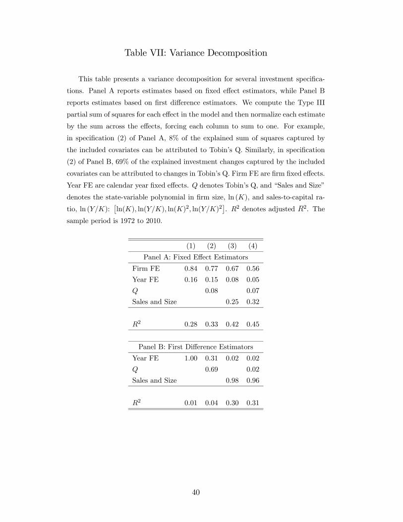
Table VII: Variance Decomposition

This table presents a variance decomposition for several investment specifica-

tions. Panel A reports estimates based on fixed effect estimators, while Panel B

reports estimates based on first difference estimators. We compute the Type III

partial sum of squares for each effect in the model and then normalize each estimate

by the sum across the effects, forcing each column to sum to one. For example,

in specification (2) of Panel A, 8% of the explained sum of squares captured by

the included covariates can be attributed to Tobin’s Q. Similarly, in specification

(2) of Panel B, 69% of the explained investment changes captured by the included

covariates can be attributed to changes in Tobin’s Q. Firm FE are firm fixed effects.

Year FE are calendar year fixed effects. Q denotes Tobin’s Q, and “Sales and Size”

denotes the state-variable polynomial in firm size, ln (K), and sales-to-capital ra-

tio, ln (Y/K):£ln(K), ln(Y/K), ln(K)2, ln(Y/K)2

¤. R2 denotes adjusted R2. The

sample period is 1972 to 2010.

(1) (2) (3) (4)

Panel A: Fixed Effect Estimators

Firm FE 0.84 0.77 0.67 0.56

Year FE 0.16 0.15 0.08 0.05

Q 0.08 0.07

Sales and Size 0.25 0.32

R2 0.28 0.33 0.42 0.45

Panel B: First Difference Estimators

Year FE 1.00 0.31 0.02 0.02

Q 0.69 0.02

Sales and Size 0.98 0.96

R2 0.01 0.04 0.30 0.31

40

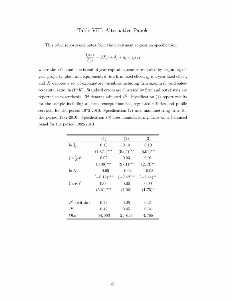
Table VIII: Alternative Panels

This table reports estimates from the investment regression specification:

Ijt+1Kjt

= βXjt + δj + ηt + εjt+1

where the left-hand-side is end-of year capital expenditures scaled by beginning-of-

year property, plant and equipment, δj is a firm fixed effect, ηt is a year fixed effect,

and X denotes a set of explanatory variables including firm size, lnK, and sales-

to-capital ratio, ln (Y/K). Standard errors are clustered by firm and t-statistics are

reported in parenthesis. R2 denotes adjusted R2. Specification (1) report results

for the sample including all firms except financial, regulated utilities and public

services, for the period 1972-2010. Specification (2) uses manufacturing firms for

the period 1982-2010. Specification (3) uses manufacturing firms on a balanced

panel for the period 1982-2010.

(1) (2) (3)

ln YK 0.13 0.10 0.10

(19.71)∗∗∗ (9.65)∗∗∗ (5.01)∗∗∗

(ln YK )

2 0.02 0.03 0.01

(8.38)∗∗∗ (9.61)∗∗∗ (2.13)∗∗

lnK −0.05 −0.02 −0.03(−8.12)∗∗∗ (−2.42)∗∗ (−2.44)∗∗

(lnK)2 0.00 0.00 0.00

(5.61)∗∗∗ (1.06) (1.75)∗

R2 (within) 0.22 0.25 0.21

R2 0.42 0.45 0.34

Obs 58, 663 25, 653 4, 788

41

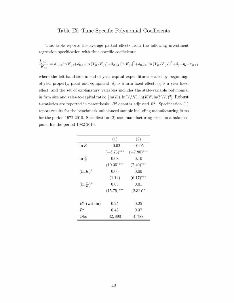
Table IX: Time-Specific Polynomial Coefficients

This table reports the average partial effects from the following investment

regression specification with time-specific coefficients:

Ijt+1Kjt

= d1,0,t lnKjt+d0,1,t ln (Yjt/Kjt)+d2,0,t [lnKjt]2+d0,2,t [ln (Yjt/Kjt)]

2+δj+ηt+εjt+1

where the left-hand-side is end-of year capital expenditures scaled by beginning-

of-year property, plant and equipment, δj is a firm fixed effect, ηt is a year fixed

effect, and the set of explanatory variables includes the state-variable polynomial

in firm size and sales-to-capital ratio:£ln(K), ln(Y/K), ln(K)2, ln(Y/K)2

¤.Robust

t-statistics are reported in parenthesis. R2 denotes adjusted R2. Specification (1)

report results for the benchmark unbalanced sample including manufacturing firms

for the period 1972-2010. Specification (2) uses manufacturing firms on a balanced

panel for the period 1982-2010.

(1) (2)

lnK −0.02 −0.05(−3.75)∗∗∗ (−7.98)∗∗∗

ln YK 0.08 0.10

(10.35)∗∗∗ (7.40)∗∗∗

(lnK)2 0.00 0.00

(1.14) (6.17)∗∗∗

(ln YK )

2 0.03 0.01

(15.75)∗∗∗ (2.32)∗∗

R2 (within) 0.25 0.25

R2 0.43 0.37

Obs 32, 890 4, 788

42

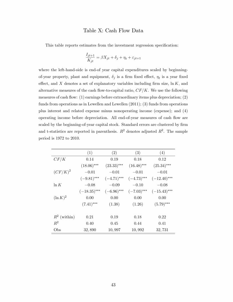
Table X: Cash Flow Data

This table reports estimates from the investment regression specification:

Ijt+1Kjt

= βXjt + δj + ηt + εjt+1

where the left-hand-side is end-of year capital expenditures scaled by beginning-

of-year property, plant and equipment, δj is a firm fixed effect, ηt is a year fixed

effect, and X denotes a set of explanatory variables including firm size, lnK, and

alternative measures of the cash flow-to-capital ratio, CF/K. We use the following

measures of cash flow: (1) earnings before extraordinary items plus depreciation; (2)

funds from operations as in Lewellen and Lewellen (2011); (3) funds from operations

plus interest and related expense minus nonoperating income (expense); and (4)

operating income before depreciation. All end-of-year measures of cash flow are

scaled by the beginning-of-year capital stock. Standard errors are clustered by firm

and t-statistics are reported in parenthesis. R2 denotes adjusted R2. The sample

period is 1972 to 2010.

(1) (2) (3) (4)

CF/K 0.14 0.19 0.18 0.12

(18.06)∗∗∗ (23.33)∗∗∗ (16.48)∗∗∗ (25.34)∗∗∗

(CF/K)2 −0.01 −0.01 −0.01 −0.01(−9.81)∗∗∗ (−4.71)∗∗∗ (−4.73)∗∗∗ (−12.40)∗∗∗

lnK −0.08 −0.09 −0.10 −0.08(−18.35)∗∗∗ (−6.96)∗∗∗ (−7.03)∗∗∗ (−15.43)∗∗∗

(lnK)2 0.00 0.00 0.00 0.00

(7.41)∗∗∗ (1.38) (1.26) (5.79)∗∗∗

R2 (within) 0.21 0.19 0.18 0.22

R2 0.40 0.45 0.44 0.41

Obs 32, 890 10, 997 10, 992 32, 731

43

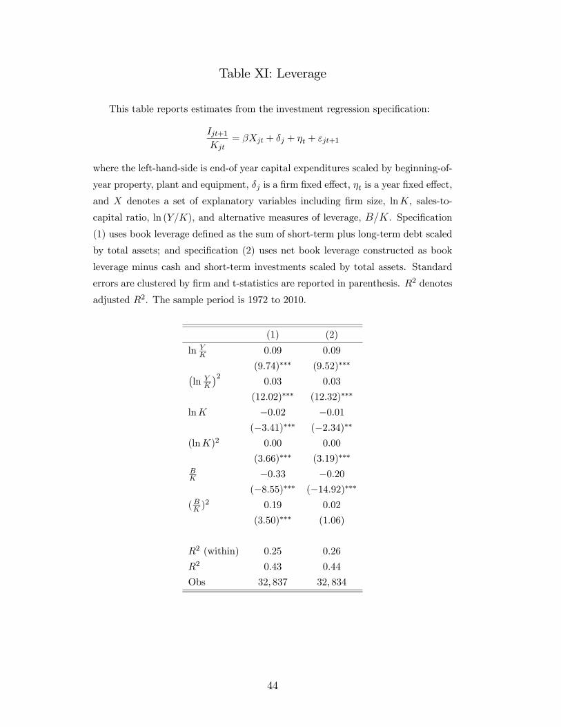
Table XI: Leverage

This table reports estimates from the investment regression specification:

Ijt+1Kjt

= βXjt + δj + ηt + εjt+1

where the left-hand-side is end-of year capital expenditures scaled by beginning-of-

year property, plant and equipment, δj is a firm fixed effect, ηt is a year fixed effect,

and X denotes a set of explanatory variables including firm size, lnK, sales-to-

capital ratio, ln (Y/K), and alternative measures of leverage, B/K. Specification

(1) uses book leverage defined as the sum of short-term plus long-term debt scaled

by total assets; and specification (2) uses net book leverage constructed as book

leverage minus cash and short-term investments scaled by total assets. Standard

errors are clustered by firm and t-statistics are reported in parenthesis. R2 denotes

adjusted R2. The sample period is 1972 to 2010.

(1) (2)

ln YK 0.09 0.09

(9.74)∗∗∗ (9.52)∗∗∗¡ln Y

K

¢20.03 0.03

(12.02)∗∗∗ (12.32)∗∗∗

lnK −0.02 −0.01(−3.41)∗∗∗ (−2.34)∗∗

(lnK)2 0.00 0.00

(3.66)∗∗∗ (3.19)∗∗∗

BK −0.33 −0.20

(−8.55)∗∗∗ (−14.92)∗∗∗

(BK )2 0.19 0.02

(3.50)∗∗∗ (1.06)

R2 (within) 0.25 0.26

R2 0.43 0.44

Obs 32, 837 32, 834

44

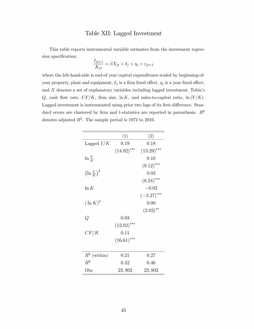
Table XII: Lagged Investment

This table reports instrumental variable estimates from the investment regres-

sion specification:Ijt+1Kjt

= βXjt + δj + ηt + εjt+1

where the left-hand-side is end-of year capital expenditures scaled by beginning-of-

year property, plant and equipment, δj is a firm fixed effect, ηt is a year fixed effect,

and X denotes a set of explanatory variables including lagged investment, Tobin’s

Q, cash flow rate, CF/K, firm size, lnK, and sales-to-capital ratio, ln (Y/K).

Lagged investment is instrumented using prior two lags of its first-difference. Stan-

dard errors are clustered by firm and t-statistics are reported in parenthesis. R2

denotes adjusted R2. The sample period is 1972 to 2010.

(1) (2)

Lagged I/K 0.19 0.18

(14.02)∗∗∗ (13.29)∗∗∗

ln YK

0.10

(9.12)∗∗∗¡ln Y

K

¢20.03

(8.24)∗∗∗

lnK −0.02(−3.27)∗∗∗

( lnK)2 0.00

(2.03)∗∗

Q 0.03

(12.02)∗∗∗

CF/K 0.11

(16.61)∗∗∗

R2 (within) 0.21 0.27

R2 0.42 0.46

Obs 23, 802 23, 802

45

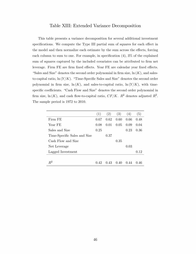
Table XIII: Extended Variance Decomposition

This table presents a variance decomposition for several additional investment

specifications. We compute the Type III partial sum of squares for each effect in

the model and then normalize each estimate by the sum across the effects, forcing

each column to sum to one. For example, in specification (4), 3% of the explained

sum of squares captured by the included covariates can be attributed to firm net

leverage. Firm FE are firm fixed effects. Year FE are calendar year fixed effects.

“Sales and Size” denotes the second order polynomial in firm size, ln (K), and sales-

to-capital ratio, ln (Y/K). “Time-Specific Sales and Size” denotes the second order

polynomial in firm size, ln (K), and sales-to-capital ratio, ln (Y/K), with time-

specific coefficients. “Cash Flow and Size” denotes the second order polynomial in

firm size, ln (K), and cash flow-to-capital ratio, CF/K. R2 denotes adjusted R2.

The sample period is 1972 to 2010.

(1) (2) (3) (4) (5)

Firm FE 0.67 0.62 0.60 0.66 0.48

Year FE 0.08 0.01 0.05 0.09 0.04

Sales and Size 0.25 0.23 0.36

Time-Specific Sales and Size 0.37

Cash Flow and Size 0.35

Net Leverage 0.03

Lagged Investment 0.12

R2 0.42 0.43 0.40 0.44 0.46

46

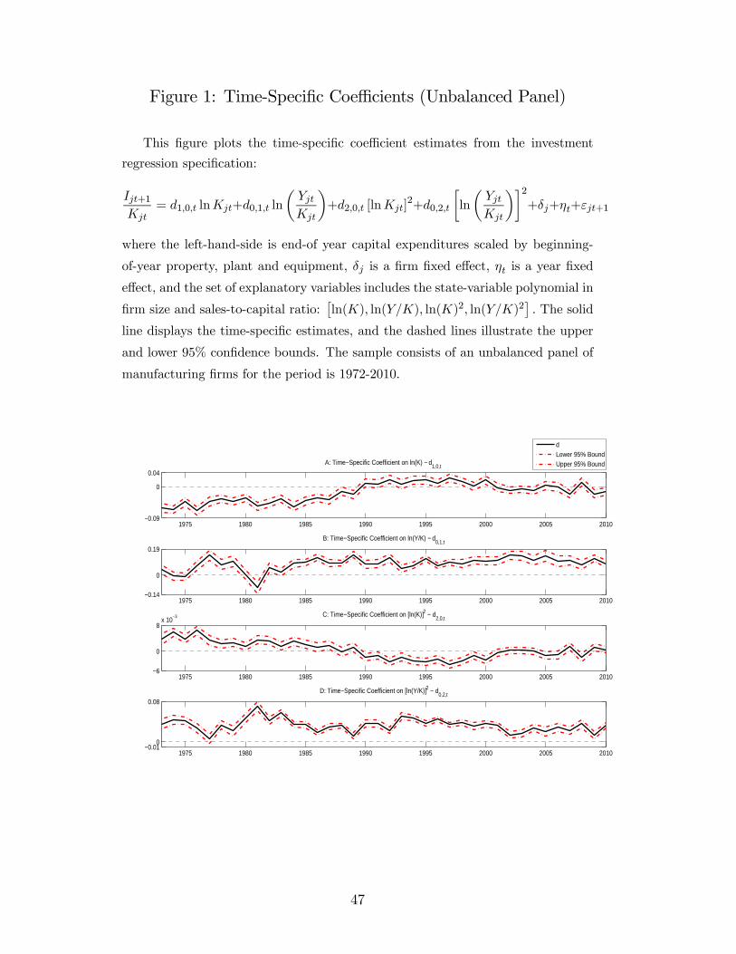
Figure 1: Time-Specific Coefficients (Unbalanced Panel)

This figure plots the time-specific coefficient estimates from the investment

regression specification:

Ijt+1Kjt

= d1,0,t lnKjt+d0,1,t ln

µYjtKjt

¶+d2,0,t [lnKjt]

2+d0,2,t

∙ln

µYjtKjt

¶¸2+δj+ηt+εjt+1

where the left-hand-side is end-of year capital expenditures scaled by beginning-

of-year property, plant and equipment, δj is a firm fixed effect, ηt is a year fixed

effect, and the set of explanatory variables includes the state-variable polynomial in

firm size and sales-to-capital ratio:£ln(K), ln(Y/K), ln(K)2, ln(Y/K)2

¤. The solid

line displays the time-specific estimates, and the dashed lines illustrate the upper

and lower 95% confidence bounds. The sample consists of an unbalanced panel of

manufacturing firms for the period is 1972-2010.

1975 1980 1985 1990 1995 2000 2005 2010−0.09

0

0.04

A: Time−Specific Coefficient on ln(K) − d1,0,t

dLower 95% BoundUpper 95% Bound

1975 1980 1985 1990 1995 2000 2005 2010−0.14

0

0.19

B: Time−Specific Coefficient on ln(Y/K) − d0,1,t

1975 1980 1985 1990 1995 2000 2005 2010−6

0

8x 10

−3 C: Time−Specific Coefficient on [ln(K)]2 − d2,0,t

1975 1980 1985 1990 1995 2000 2005 2010−0.01

0

0.08

D: Time−Specific Coefficient on [ln(Y/K)]2 − d0,2,t

47

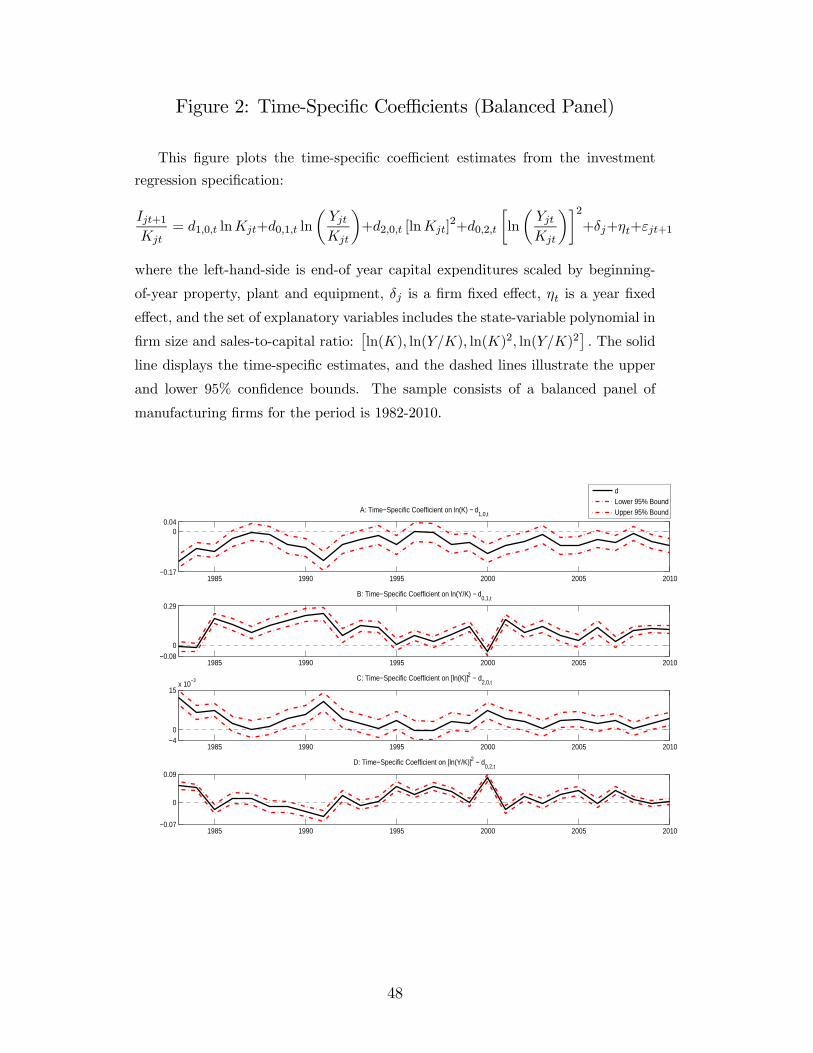
Figure 2: Time-Specific Coefficients (Balanced Panel)

This figure plots the time-specific coefficient estimates from the investment

regression specification:

Ijt+1Kjt

= d1,0,t lnKjt+d0,1,t ln

µYjtKjt

¶+d2,0,t [lnKjt]

2+d0,2,t

∙ln

µYjtKjt

¶¸2+δj+ηt+εjt+1

where the left-hand-side is end-of year capital expenditures scaled by beginning-

of-year property, plant and equipment, δj is a firm fixed effect, ηt is a year fixed

effect, and the set of explanatory variables includes the state-variable polynomial in

firm size and sales-to-capital ratio:£ln(K), ln(Y/K), ln(K)2, ln(Y/K)2

¤. The solid

line displays the time-specific estimates, and the dashed lines illustrate the upper

and lower 95% confidence bounds. The sample consists of a balanced panel of

manufacturing firms for the period is 1982-2010.

1985 1990 1995 2000 2005 2010−0.17

00.04

A: Time−Specific Coefficient on ln(K) − d1,0,t

dLower 95% BoundUpper 95% Bound

1985 1990 1995 2000 2005 2010−0.08

0

0.29

B: Time−Specific Coefficient on ln(Y/K) − d0,1,t

1985 1990 1995 2000 2005 2010−4

0

15x 10

−3 C: Time−Specific Coefficient on [ln(K)]2 − d2,0,t

1985 1990 1995 2000 2005 2010−0.07

0

0.09

D: Time−Specific Coefficient on [ln(Y/K)]2 − d0,2,t

48