Embed Size (px)
Citation preview

Beyond Standard Model Physics
March 18, 2013
Tuomas Hapola
Institut for Fysik, Kemi og Farmaci
Particle Physics & Origin of Mass
CP - Origins3
Academic Advisor: Prof. Francesco Sannino
A dissertation submitted to the University of Southern Denmark
for the degree of Doctor of Philosophy

ii
iii
Abstract
One era came to an end 4th of July last year when two experiments
at the Large Hadron Collider announced the discovery of a resonance
consistent with the properties of the Standard Model Higgs boson. The
Higgs boson was the last missing piece of the Standard Model and after
it mass is unambiguously measured, all the nineteen free parameters of
the model are fixed. Although the Standard Model is in agreement with
a great number of experimental measurements, it cannot explain all the
observations.
In this thesis we investigate extensions of the Standard Model where
the standard Higgs sector is replaced by a strongly interacting sector.
We begin with a brief introduction to the Standard Model and review the
reasons why there must be something beyond the Standard Model. After
developing tools to study strongly interacting theories, we continue with
the Minimal Walking Technicolor model and examine how it possibly
manifests itself at the Large Hadron Collider.
The last chapter of the thesis in devoted to an extension which only
adds more particles on top of the Standard Model. One of the new
particle is stable and electrically neutral explaining the existence of
a type of matter in the universe which does not shine light i.e. dark
matter.

iv

v
Resume
En æra sluttede i den 4. juli sidste ar, da to eksperimenter pa Large
Hadron Collider annoncerede opdagelsen af en resonans i overensstem-
melse med egenskaber af Standardmodellens Higgs boson. Med malingen
af Higgsbosonens masse er alle Standarmodellens nitten frie parametre
fastlagt. Standardmodellen er med høj præcision i overensstemmelse
med et stort antal af observabler ved forskellige energi-skalaer.
I denne afhandling undersøger vi udvidelser af standardmodellen,
hvor standard Higgs sektor erstattes af en stærkt vekselvirkende sektor.
Vi begynder med en kort introduktion til Standardmodellen og gennemga
arsagerne til, at der ma være noget ud over Standardmodellen. Efter
udviklingen af værktøjer til at studere stærkt vekselvirkende teorier,
fortsætter vi med Minimal Walking Technicolor modellen og undersøger,
hvordan det muligvis manifesterer sig ved Large Hadron Collider.
Det sidste kapitel i afhandlingen er dedikeret til en forlængelse, som
kun tilføjer flere partikler i forlængelse af Standardmodellen. En af de
nye partikler, der er stabil og elektrisk neutral, forklarer eksistensen af
en slags stof i Universet, som ikke skinner lys.

vi

vii
Preface
The research for this thesis was done at the Centre for Cosmology and Particle Physics
Phenomenology (CP3-Origins), University of Southern Denmark. I would like to thank
my advisor Francesco Sannino for the opportunity to do this PhD in Odense, and for all
the guidance during these years. I would also like to thank all the people in CP3 for the
encouraging working atmosphere.
Finally, I would like express my deepest gratitude to Krista for her love, support and
patience.
Tuomas Hapola

viii

ix
List of Publications
The following publications are included in the thesis:
I Pseudo Goldstone Bosons Phenomenology in Minimal Walking Techni-
color
T. Hapola, F. Mescia, M. Nardecchia and F. Sannino
Eur. Phys. J. C72, 2063 (2012) [arXiv:1202.3024 [hep-ph]]
II W’ and Z’ limits for Minimal Walking Technicolor
J. R. Andersen, T. Hapola and F. Sannino
Phys. Rev. D85, 055017 (2011) [arXiv:1105.1433 [hep-ph]]
III Composite Higgs to two Photons and Gluons
T. Hapola and F. Sannino
Mod. Phys. Lett. A26, 2313 (2011) [arXiv:1102.2920 [hep-ph]]
IV Perturbative Extension of the Standard Model with 125 GeV Higgs and
Magnetic Dark Matter
K. Dissauer, M. T. Frandsen, T. Hapola and F. Sannino
Accepted for publication in Phys. Rev. D [arXiv:1211.5144 [hep-ph]]

x

Contents
1. Introduction 3
2. Introduction to Elementary Particle Physics 5
2.1. Symmetries . . . . . . . . . . . . . . . . . . . . . . . . . . . . . . . . . . 5
2.2. Goldstone’s Theorem . . . . . . . . . . . . . . . . . . . . . . . . . . . . . 8
2.3. Superconductivity . . . . . . . . . . . . . . . . . . . . . . . . . . . . . . . 10
2.4. Standard Model . . . . . . . . . . . . . . . . . . . . . . . . . . . . . . . . 11
2.4.1. Custodial symmetry . . . . . . . . . . . . . . . . . . . . . . . . . 14
2.4.2. Comments . . . . . . . . . . . . . . . . . . . . . . . . . . . . . . . 16
2.5. Going Beyond . . . . . . . . . . . . . . . . . . . . . . . . . . . . . . . . . 17
2.5.1. Empirical proof . . . . . . . . . . . . . . . . . . . . . . . . . . . . 17
2.5.2. Theoretical Arguments . . . . . . . . . . . . . . . . . . . . . . . . 17
2.5.3. Something potentially dangerous . . . . . . . . . . . . . . . . . . 18
2.5.4. How to go Beyond . . . . . . . . . . . . . . . . . . . . . . . . . . 20
3. QCD and Chiral Symmetry Breaking 21
3.1. Effective Lagrangian . . . . . . . . . . . . . . . . . . . . . . . . . . . . . 23
3.2. Banks-Casher Relation . . . . . . . . . . . . . . . . . . . . . . . . . . . . 25
3.3. Vafa-Witten Theorem . . . . . . . . . . . . . . . . . . . . . . . . . . . . 26
3.4. Gauging . . . . . . . . . . . . . . . . . . . . . . . . . . . . . . . . . . . . 29
3.5. Vacuum Alignment . . . . . . . . . . . . . . . . . . . . . . . . . . . . . . 29
3.6. Weinberg Sum Rules . . . . . . . . . . . . . . . . . . . . . . . . . . . . . 33
4. Technicolor 35
4.1. Historical Setup . . . . . . . . . . . . . . . . . . . . . . . . . . . . . . . . 36
4.2. Extended technicolor and Walking . . . . . . . . . . . . . . . . . . . . . . 37
xi

Contents 1
5. Minimal Walking Technicolor 47
5.1. Goldstone Bosons . . . . . . . . . . . . . . . . . . . . . . . . . . . . . . . 48
5.1.1. Effective Theory . . . . . . . . . . . . . . . . . . . . . . . . . . . 48
5.1.2. Results . . . . . . . . . . . . . . . . . . . . . . . . . . . . . . . . . 53
5.1.3. Summary . . . . . . . . . . . . . . . . . . . . . . . . . . . . . . . 54
5.2. Vector Resonances . . . . . . . . . . . . . . . . . . . . . . . . . . . . . . 54
5.2.1. Non-linear Lagrangian . . . . . . . . . . . . . . . . . . . . . . . . 55
5.2.2. Linear Lagrangian . . . . . . . . . . . . . . . . . . . . . . . . . . 57
5.2.3. Comparison . . . . . . . . . . . . . . . . . . . . . . . . . . . . . . 58
5.2.4. Results . . . . . . . . . . . . . . . . . . . . . . . . . . . . . . . . . 59
5.2.5. Summary . . . . . . . . . . . . . . . . . . . . . . . . . . . . . . . 61
5.3. Technicolor Higgs . . . . . . . . . . . . . . . . . . . . . . . . . . . . . . . 63
5.3.1. Hybrid Model . . . . . . . . . . . . . . . . . . . . . . . . . . . . . 63
5.3.2. Results . . . . . . . . . . . . . . . . . . . . . . . . . . . . . . . . . 64
5.3.3. Summary . . . . . . . . . . . . . . . . . . . . . . . . . . . . . . . 65
6. Dark Matter Model Building 67
6.1. The model . . . . . . . . . . . . . . . . . . . . . . . . . . . . . . . . . . . 67
6.2. Results . . . . . . . . . . . . . . . . . . . . . . . . . . . . . . . . . . . . . 69
6.3. Summary . . . . . . . . . . . . . . . . . . . . . . . . . . . . . . . . . . . 70
A. Witten Anomaly 71
B. Dyson-Schwinger Equation 75
Bibliography 83
List of Figures 89
List of Tables 91

2

Chapter 1.
Introduction
The Large Hadron Collider (LHC) is the biggest scientific instrument ever created. It
accelerates and collides protons along the 27 kilometers long tunnel excavated beneath
the Franco-Swiss border. In addition to the main accelerator, several other smaller
machines are needed to inject the protons into the LHC. Protons, which result from
hydrogen atoms by removing electrons, are first accelerated in the linear collider. From
the linear collider, protons are injected into the proton-booster synchrotron, followed
by the proton synchrotron and the super proton synchrotron. From the super proton
synchrotron, protons with 450 GeV energy are finally injected into the LHC. Protons are
then accelerated to obtain the wanted collision energy.
Proton beams consist of 2808 bunches with 1.15 · 1011 protons in each bunch. At the
collision point, the transverse size of both beams is squeezed to a size of tens of microns.
Together with bunch crossing interval of the order of tens of nano seconds this should
yield an instantaneous luminosity up to 1034 cm−2s−1. High instantaneous luminosity
and frequent collision rate are desired to be able to study rare processes. The downside
is that there will be tens of simultaneous events per bunch crossing i.e. events are piling
up.
When two protons collide they break apart into quarks and gluons. High energy
collision of these quarks and gluons carrying a small fraction of the total collision energy
is what we are actually interested in, and what we can calculate using the Standard
Model (SM). This hard process is accompanied by low momentum transfer processes and
the experimental challenge is to pin down what happens in the hard interaction.
The main physics goal of the LHC is to complete the dynamical picture of the SM. A
first step towards this goal was taken when the two biggest experiments, ATLAS and
3

4 Introduction
CMS, announced the discovery of a resonance consistent with the properties of the SM
Higgs boson [1, 2]. This particle was the final missing piece of the SM and after its mass
is measured, all the nineteen free parameters of the SM are fixed. The next big step is to
find out what lies beyond the SM. Despite of its success it cannot accommodate all the
observations and there are a number of theoretical reasons why it cannot be the ultimate
theory of nature.
This thesis consists of four original research papers [I-IV] and an introductory and
summary parts presented below. In Chapter 2, the SM of the particle physics and its
problems are discussed. The chapter begins with a discussion about the symmetries
and why the symmetries are the primary reason for the predictive power of the SM. In
Chapter 3, we introduce chiral symmetry breaking using the quantum chromodynamics
(QCD) as an example. Chapter 4 gives an introduction to Technicolor and Chapter 5
summarizes the results of papers [I-III]. The last Chapter 6 introduces the Dark Matter
problem and summarizes the results of paper [IV].

Chapter 2.
Introduction to Elementary Particle
Physics
2.1. Symmetries
Symmetry means invariance under a set of transformations. For, example a square is a
symmetric geometric object which looks exactly the same if we rotate it by an angle of
90 degrees, or by n ∈ Z times this angle. The set of all symmetry transformations form
a symmetry group of the object. Of course, not all transformations are symmetric. A
rotation is a continuous transformation, but we could have used a discrete transformation
as an example as well.
Similarly, the laws of nature can be symmetric. This means the form of the equations
describing the law is maintained under a change of variables and/or space-time coordinates.
Hence, it is natural to categorize the symmetries accordingly to geometric symmetries
and internal symmetries. The geometric symmetries act on space-time coordinates and
the internal symmetries do not act on them.
We can relate the continuos symmetries of the equation of motions to conserved
quantities. The precise mathematical formulation of this is given by the Noether’s
theorem [3].
Theorem. (Noether) If the equations of motion are invariant under a continuous trans-
formation with n parameters, there exist n conserved quantities.
This applies to both geometric and internal symmetries.
5

6 Introduction to Elementary Particle Physics
In classical mechanics the basic space time dependent transformations are translation
in time, translations in space and rotations in space. If the equations of motion are invari-
ant under these transformations, the corresponding conserved quanties, or conservation
laws, are
Time independence → Energy conservation
Translation independence → Momentum conservation
Rotational independence → Angular momentum conservation
In order to discuss the relativistic particles, it is convenient to introduce Minkowski
spaceM which is a real 4-dimensional vector space parametrized by coordinates xµ = (t, ~r)
and equipped with the metric
(ds)2 = (dx)2 = dt2 − (d~r)2. (2.1)
The Lorentz transformations x→x′ = Λx and the space-time translations x→x′ = x+ a
(a ∈M) both form a group of transformations leaving the Minkowski metric invariant. A
semi-direct product1 of these groups form the group of isometries of Minkowski space-time,
called the Poincare group.
Describing an elementary particle should not depend on its position in space-time
or if the observer is in uniform motion relative to it. Thus, all the elementary particles
can be classified according to representations of the Poincare group. Moreover, the
mathematical description of a particle and its interactions should be invariant under the
Poincare group.
Let us write down a Lagrangian which is invariant under the Poincare transformations
L = ψ(iγµ∂µψ) = ψ(i/∂ψ). (2.2)
It describes a Dirac fermion ψ(x) and is in addition invariant under a global U(1) phase
transformation
ψ(x)→ eieαψ(x), (2.3)
where e and α are space-time independent constants. If we take the α to be a space-time
dependent function, equation (2.3) is no longer invariant under the U(1) transformation.
1The group of translations is Abelian.

Introduction to Elementary Particle Physics 7
In order to restore the invariance, we replace the partial derivative with the covariant
derivative
Dµ = ∂µ + ieAµ, (2.4)
where the gauge field Aµ transforms as
Aµ→Aµ − ∂µα(x). (2.5)
Local phase transformations are called gauge transformations and the invariance under
these transformations is known as gauge invariance. The procedure is called gauging and
it fixes the form of interactions. The local, and also global, U(1) symmetry is a continuous
symmetry and the corresponding conserved quantity, in this case, is the electric charge.
This can be generalized to non-abelian compact Lie groups. It is important to note the
role of internal and space time symmetries.
The internal and space-time symmetries are described in terms of Lie groups. There is
no non trivial way to combine these symmetries according to Coleman-Mandula theorem
[4]. If we consider a more general algebraic structure than a Lie group, namely a graded
Lie group, this can be omitted. The Haag-Lopuszanski-Sohnius theorem [5] states that
the most general graded Lie group of symmetries of a local field theory is the N-extended
super Poincare group. This allows non trivial mixing between internal and space-time
symmetries leading to symmetry relating bosons and fermions.
Up to this point, we have considered only exact symmetries. Later, it will be important
to differentiate what actually is symmetric, Lagrangian or the solutions, and at what
scale the symmetry manifests itself and, if broken, how it is broken.
Explicit breaking can occur via non-invariant terms in the Lagrangian. This does not
mean that the symmetry cannot be used to draw conclusions if the breaking is small.
Some of the Lagrangian’s classical symmetries can be spoiled by the quantum effects.
This is called an anomalous breaking and the term driving the breaking is called an
anomaly. It is important that in the end all the anomalies are cancelled. Otherwise
the renormalizability of the theory is destroyed. If the Lagrangian is more symmetric
than the quantum states, the symmetry is said to be spontaneously broken. Especially
interesting is if the vacuum is not invariant under the same symmetries as the Lagrangian.

8 Introduction to Elementary Particle Physics
2.2. Goldstone’s Theorem
Consider an action which is invariant under the infinitesimal transformation
φi→φ′i = φi + θa(δφ)αi , (2.6)
where , for generality, φi can be either fermonic or bosonic. Following from the Noether’s
theorem, we have a conserved charge
Qa(t) =
∫d3xJa0 (x), (2.7)
where the corresponding current is
Jaµ(x) = − δLδ(∂µφi)
(δφ)ai . (2.8)
Let us take a small side step at this point for further convenience. The conjugate
field is defined as
πi(x) =δLδ∂0φi
. (2.9)
Using the canonical commutation relations, or the anti-commutation relations in the
fermion case,
[πi(~x, t), φj(~y, t)] = −iδ3(~x− ~y)δij, (2.10)
one can show that the conserved charges generate the algebra
[Qa(t), Qb(t)] = ifabcQc(t). (2.11)
From this relation, it follows that also the unintegrated currents satisfy
[Ja0 (~x, t), J b0(~x, t)] = ifabcJ c0(~x, t)δ3(~x− ~y). (2.12)
This is the basis of current algebra which was extensively employed during the early
days of modern particle physics.

Introduction to Elementary Particle Physics 9
Let Q be a symmetry charge, and the corresponding conserved current Jµ, so that
Q|0〉 6= 0 (2.13)
The vacuum state |0〉 is not annihilated by Q and therefore does not represent the true
vacuum of the theory. Current conservation implies that
0 =
∫d3x [∂µJ
µ(x), φ(0)]
= ∂0
∫d3x
[J0(x), φ(0)
]+
∫S
d~S[~J(x), φ(0)
],
(2.14)
for the field φ(0). We take the surface S to be large enough so that the last term vanishes.
This gives
d
dt[Q(t), φ(0)] = 0. (2.15)
Then
〈0| [Q(t), φ(0)] |0〉 = C 6= 0, (2.16)
which, after inserting a complete set of intermediate states and integrating over ~x gives∑n
(2π)3δ3(~pn)[〈0|J0(0)|n〉〈n|φ(0)|0〉e−iEnt − 〈0|φ(0)|n〉〈n|J0(0)|0〉eiEnt
]= C 6= 0.
(2.17)
Now, if En 6= 0 the opposite frequency parts cannot cancel and the expression cannot be
constant. In order to satisfy the previous equation the intermediate states have to be
massless. The existence of these states is proven by the fact that C 6= 0. Thus for every
broken generator there must be massless state satisfying
〈n|φ(0)|0〉 6= 0, 〈0|J0(0)|n〉 6= 0. (2.18)
This result is called the (Nambu-)Goldstone’s theorem [6].
10 Introduction to Elementary Particle Physics
2.3. Superconductivity
The original motivation to formulate the Higgs mechanism came from condensed matter
physics and superconductivity. This section serves as an introduction to spontaneous
symmetry breaking and will also be used later on to motivate the idea of dynamical
electroweak symmetry breaking.
Superconductivity is the phenomenon of vanishing electrical resistivity at low tem-
peratures and expulsion of magnetic fields from the interior of the sample (the Meissner
effect). This phenomenon can be described near the critical temperature, Tc, with
the Ginzburg-Landau model which is a generalization of the Landau model for phase
transitions.
Let us begin with a Lagrangian
L = −1
4F 2µν + |(∂µ + iqAµ)φ|2 +m2|φ|2 + λ|φ|4, (2.19)
which couples a complex scalar field φ to Maxwell’s theory [7]. This Lagrangian is
invariant under local U(1) phase rotations. In the static limit, (2.19) reduces to the
Ginzburg-Landau Lagrangian
L =1
2(∇×A)2 + |(∇− iqA)φ|2 +m2|φ|2 + λ|φ|4, (2.20)
where m2 = a(T − Tc) near the critical temperature. Above the critical temperature
m2 > 0 and the minimum of the potential is at |φ| = 0. When the temperature is below
the critical one, the minimum is at |φ|2 = −m2
2λ. The Vacuum is not anymore invariant
under U(1) rotations, which in the static limit are
φ(x)→ eiα(x)φ(x), ~A→ ~A+i
q∇α(x). (2.21)
The conserved current, associated with U(1) rotations, is
~j = −i (φ∗∇φ− φ∇φ∗)− 2q|φ|2 ~A. (2.22)
When T < Tc and the field φ varies slowly over the medium:
~j = −qm2
2λ~A ≡ −k2 ~A. (2.23)
Introduction to Elementary Particle Physics 11
This is called the London equation. The Ohm’s law
~E = R~j (2.24)
defines the resistance R. From the London equation and current conservation one can
deduce that the resistance R must be zero. Thus, we have superconductivity. The
Meissner effect can be derived taking the curl of Ampere’s equation
∇× (∇× ~B) = ∇(∇ ·∇)−∇2 ~B = ∇×~j, (2.25)
⇒ ∇2 ~B = k2 ~B, (2.26)
where we have used Gauss law. In one dimension Bx∼ e−kx, indicating that the magnetic
fields are expelled from a superconductor with penetration depth characterized by 1/k.
By writing equation (2.26) in a covariant form
2Aµ = −k2Aµ, (2.27)
we can see that the photon has acquired a mass k.
This behavior can be explained in terms of a microscopic theory known as the BCS
theory of superconductivity [8]. The main assumption of the BCS theory is that there
exists an attractive force between the electrons inside the medium. Thus, the electrons
will pair and form a bound state called the Cooper pair. At low temperatures these
fall into the same quantum state forming a Bose-Einstein condensate. In this case, the
complex φ above would be a many particle wave function. The coefficients m2 and λ can
be calculated from the BCS theory which effectively coincides with the Ginzburg-Landau
model near the phase transition. The attractive interaction arises when the electron
phonon interactions overcome the repulsive Coulomb interaction. The nuclei in a crystal
oscillate about their equilibrium positions and the quanta of these vibrations are the
phonons.
2.4. Standard Model
The Standard Model (SM) of particle physics is a gauge field theory based on the
gauge symmetry group SU(3)×SU(2)L×U(1)Y [9–11]. The field content of the SM is
summarized in Table 2.1 The following notation is used:

12 Introduction to Elementary Particle Physics
Gauge Fields
Symbol Associate charge Group Coupling Representation
B Weak hypercharge U(1)Y g′ (1,1, 0)
W Weak isospin SU(2)L g (1,3, 0)
G color SU(3) gs (8,1, 0)
Fermions
Symbol Name Baryon number Lepton number Representation
QL Left-handed quark 13
0 (3,2, 13)
(uc)iL Right-handed up quark 13
0 (3,1,−43)
(dc)iL Right-handed down quark 13
0 (3,1, 23)
LL Left-handed lepton 0 1 (1,2,−1)
(ec)iL Right-handed lepton 0 1 (1,1, 2)
Scalars
Symbol Name Representation
H Higgs boson (1,2, 1)
Table 2.1.: The field content of the SM.
QiL =
uidi
L
LiL =
νieei
L
, (2.28)
where u(d) is called an up(down) type quark, e a lepton, νe a neutrino and i is the
generation index. The SM contains three generations with a naming convention:
u ∈ {u, c, t},
d ∈ {d, s, b},
e ∈ {e, µ, τ},
νe ∈ {νe, νµ, ντ}.
For further convenience the Lagrangian of the SM is useful to divide into four parts:
LSM = LGauge + LKinetic + LHiggs + LYukawa. (2.29)

Introduction to Elementary Particle Physics 13
The first term contains kinetic terms for the gauge bosons
LGauge = −1
4BµνB
µν − 1
4W iµνW
iµν − 1
4W aµνW
aµν , (2.30)
where
Bµν = ∂µBν − ∂νBµ, (2.31)
W iµν = ∂µW
iν − ∂νW i
µ + gεijkW jµW
kν , (2.32)
Gaµν = ∂µG
aν − ∂νGa
µ + gsfabcGb
µGcν . (2.33)
The structure constants are defined as [τ i, τ j] = iεijkτ k and [λa, λb] = ifabcλc, where τ i
and λa are the generators of SU(2) and SU(3) groups respectively. The second term
contains kinetic terms for the fermions
L = QLi /DQL + uRi /DuR + dRi /DdR + LLi /DLL + eRi /DeR, (2.34)
where the covariant derivative is
Dµ = ∂µ − ig′Y Bµ − igτ i
2W iµ − igs
λa
2Gaµ. (2.35)
Here Y denotes the hypercharge of a respective particle. Of course the last two terms in the
covariant derivative can be absent if the particle is not charged under the corresponding
force.
At this stage all the fermions are massless. A Majorana mass term is not possible
because all the fermions carry hypercharge. A Dirac mass term is not allowed because
the left-handed and right-handed fermions are not in complex conjugated representations.
Thus the fermion sector possesses five accidental global U(3) symmetries for the right
and left-handed quarks and leptons.
The Yukawa Lagrangian violates these symmetries
LY = −Y iju Q
iLεHu
jR − Y
ijd Q
iLHd
jR − Y
ije L
iLHe
jR + h.c., (2.36)
where Yu, Yd and Ye are 3× 3 matrices and
H =
h+
h0
. (2.37)

14 Introduction to Elementary Particle Physics
is the Higgs doublet. A subset of [U(3)]5 symmetries is left intact corresponding to
the baryon and lepton numbers. In the end, only a linear combination of these two
symmetries is an accidental global symmetry of the SM, separately these symmetries are
anomalously broken. When the Higgs field acquires a vacuum expectation value (vev),
〈H〉 =
0
v
, (2.38)
the Yukawa interactions form mass terms for the fermions. The neutrinos are still
massless because the minimal SM does not contain right-handed neutrinos. Formation
of a Majorana mass term after the symmetry breaking is forbidden by the accidental
baryon minus lepton number symmetry.
The last part of the Lagrangian is the part containing only the Higgs and the
electroweak gauge bosons
LH = (DµH)†DµH − V (H),
V (H) = −µ2H†H + λ(H†H
)2,
(2.39)
where the covariant derivative is
Dµ = ∂µ + ig
2σ ·Wµ + i
g′
2Bµ. (2.40)
The mass terms for the gauge bosons follow from the kinetic term after the Higgs field
acquires the vev.
2.4.1. Custodial symmetry
The Higgs Lagrangian is SU(2)L×U(1)Y invariant by construction, but has also an
accidental symmetry. To illustrate better this accidental symmetry we can write the
Lagrangian in another form. Instead of a doublet, let us form a bi-doublet:
Φ =
h0∗ h+
−h− h0
. (2.41)

Introduction to Elementary Particle Physics 15
Now we can write the Higgs Lagrangian as
LH = Tr (DµΦ)†DµΦ + µ2TrΦ†Φ− λ(TrΦ†Φ
)2, (2.42)
where the covariant derivative is
Dµφ = ∂µΦ + ig
2σ ·WµΦ− ig
′
2BµΦσ3. (2.43)
The electroweak symmetry acts as follows
SU(2)L : Φ→LΦ,
U(1)Y : Φ→Φe−i2σ3θ.
(2.44)
We can make the global symmetry manifest by taking the hypercharge interactions to
vanish, g′→ 0. In this limit the Higgs Lagrangian has a global SU(2)R symmetry
SU(2)R : Φ→ΦR†. (2.45)
Therefore the Higgs Lagrangian has SU(2)L×SU(2)R symmetry which breaks down to
SU(2)L+R when the Higgs field aquires a vev
〈Φ〉 =1√2
v 0
0 v
. (2.46)
This breaking pattern yields three Goldstone bosons which are eaten by the Higgs
mechanism providing masses to the weak gauge bosons.
M2W =
1
4g2v2
M2Z =
1
4(g2 + g′2)v2.
(2.47)
Thus, at tree level
ρ =M2
W
M2Z cos2 θW
= 1, (2.48)
where the θW is the Weinberg angle. In the limit g′→ 0 the W+, W− and Z bosons
form a triplet under the SU(2)L+R explaining why the masses are degenerate in this

16 Introduction to Elementary Particle Physics
limit. Notably the radiative corrections must be proportional to g′2 protecting the tree
level value ρ = 1. For this reason this symmetry is called the custodial symmetry.
2.4.2. Comments
There are a few notes which should be kept in mind for later reference. The theory is
not invariant under axial gauge transformations and one has to check that the gauge
anomalies are cancelled. The gauge anomaly cancellation is shown in many quantum
field theory text books (see, for example, [7]). Because of the SU(2)L gauge group, the
SM suffers also from the Witten topological anomaly, reviewed in Appendix A. This
anomaly cancels because there is an even number of left-handed fermion doublets in the
theory.
There is no reason for the Yukawa couplings in equation (2.36) to be diagonal.
These matrices can be brought to diagonal form using bi-unitary transformations. The
electromagnetic and neutral weak currents will remain intact under the diagonalization
and there is no flavor changing neutral currents. This is easily seen as all generations
are replicas of each other and unitary diagonalization matrices always give rise to the
unit matrix. Also, the charged current for the leptons is flavor diagonal provided that
the neutrinos are mass degenerate. This is true in the SM. Only the system of charged
weak currents involving quarks is effected by the mixing. The non-existence of the flavor
changing neutral currents in the SM is called the GIM mechanism [12]. Nowadays it
looks trivial, but back in the day it was proposed only three quarks were thought to exist
and it predicted the charm quark.
The gauge structure SU(2)L×U(1)Y and the electroweak sector was tested thoroughly
at the Large Electron-Positron collider (LEP). Colliding electron- positron pairs at the
Z-pole enabled the precise measurements of several observables [13]. These precision
observables agree well with the theoretical predictions. By doing a global fit one can
examine how consistent the theory is or determine the validity of the model by over
constraining the system. This is now possible because we know the Higgs mass [14].

Introduction to Elementary Particle Physics 17
2.5. Going Beyond
Before discussing different strategies and ways to go beyond the standard model, it is
necessary to discuss why there should be something more than the SM. I will first list
some examples of observations which are not explained within the SM and then give a
few theoretical arguments.
2.5.1. Empirical proof
The first solid result which requires something beyond the SM is that neutrinos must
be massive because they are observed to oscillate. The most minimal extension of the
SM would be to add right-handed neutrinos when one would be able to write down
Majorana mass terms for neutrinos or/and Yukawa interactions. It is interesting to
point out that the most stringent limits on the neutrino mass scale comes from the
cosmological measurements [15] and not from the dedicated neutrino experiments. The
neutrino experiments, which study neutrino oscillations, can access only to the mass
differences [16].
The next observational evidence does not come from the particle physics experiments
but from the cosmology (see for example [17]). Only roughly five percents of the
energy content of the universe is made up of ordinary matter. Dark energy accounts
approximately 72 percents and dark matter (DM) circa 23 percents. We do not know
much about dark energy. The same applies for DM but at least we know that it behaves
gravitationally like ordinary matter but does not shine light, which is where the name
comes from.
2.5.2. Theoretical Arguments
At the Planck scale around 1019 GeV, gravity becomes a strong force. Due to the
non-renormalizabilty of gravity, the SM can be at most an effective theory up to the
Planck scale. Once we have accepted the existence of a cut-off, we run into problems. The
radiative corrections to the Higgs mass diverge quadratically with this high energy cut-off
driving theory to be strongly coupled because λH ∼m2H/v
2. The quadratic corrections
and the huge hierarchy between the electroweak scale v ≈ 246 GeV and the Planck
scale implies that there must be new physics at lower scales to meet the observed Higgs

18 Introduction to Elementary Particle Physics
mass. Otherwise, one must unnaturally fine-tune the Higgs mass order by order so
that the physical mass is the observed one. To this respect the experimental success of
the SM is unreasonable.
One could also ask that, why there is only one scalar field and three families of
fermions. The hierarchy in the fermion masses is also an interesting question. Without
prior knowledge one would expect the masses to be in the order of the electroweak scale.
Only the top quark mass fits this expectation.
2.5.3. Something potentially dangerous
Let us examine two potential problems, namely triviality and the vacuum stability. The
Higgs self-coupling runs as a function of the renormalization scale µ as [18]
dλ
dt= βλ, (2.49)
where t = lnµ. At one-loop the beta function reads
βλ =3
4π2
[λ2 +
1
2λy2
t −1
4y4t −
1
8λ(3g2 + g′2) +
1
64(3g4 + 2g2g′2 + g′4)
], (2.50)
where yt is the top quark Yukawa coupling. Studying two different regimes λ >> g, g′, yt
and λ << g, g′, yt we can set both a lower and upper bound on the Higgs mass.
Let us consider first the regime λ >> g, g′, yt. At this limit it is straightforward to
solve equation (2.49)
λ(µ) =λ(v)
1− 3λ(v)4π2 ln
(µ2
v2
) . (2.51)
The self coupling will hit a Landau pole at the scale µ = ve2π/3λ(v). This allows us to
determine λmax(v) by taking λ(µ) =∞. This yields
λmax(v) =4π2
3 ln(µ2
v2
) (2.52)

Introduction to Elementary Particle Physics 19
The Higgs mass is related to the self-coupling through the relation m2h = 2λv2. Plugging
in the maximum value for the self coupling gives:
mh <
√√√√ 8π2v2
3 ln(µ2
v2
) . (2.53)
Using the Planck mass as a cut-off for the theory, the numerical value of the upper limit
is mh < 160 GeV.
The lower limit is set by examine the region λ << g, g′, yt. The electroweak vacuum
must be lower than the symmetric vacuum and it must be bounded below. The beta
function in this region is given as
βλ =1
16π2
[−3y4
t +3
16
(2g4 + (g2 + g′2)2
)]=
3
16π2v4
[2m4
W +m4Z − 4m4
t
]. (2.54)
This is clearly negative and thus the vacuum is stable until the scale when λ(µ) < 0.
Requiring λ(µ) > 0 we obtain a condition
λ(v) + βλ ln
(µ2
v2
)> 0. (2.55)
Again, using the relation between the self-coupling and the Higgs mass we get
m2h > −2v2βλ ln
(µ2
v2
). (2.56)
If we now plug in the numbers, we find that the lower bound is actually larger than the
upper bound. The one loop result thus does not make any sense. A more careful analysis
using a 2-loop renormalization group improved effective potential suggests that we are
currently just below the lower bound for stability [19].
Notice that the uncertainties are still sizable; mainly coming from the Higgs mass
and from the top quark mass uncertainties. Even if the Higgs potential is not absolutely
stable, it is enough if the decay time to another vacuum is longer than the age of the
universe.

20 Introduction to Elementary Particle Physics
2.5.4. How to go Beyond
As we saw in the last section we have some solid observational reasons to extend the SM.
The theoretical problems are more difficult to use as a guiding principle. There is no
theorem which states that nature should respect conceptual nicety. I would like to get
rid of these problems. However, one must consider that after the discovery of the Higgs,
and if it is confirmed to be SM like, one could argue that maybe these are not so severe
after all. Even if there is a more fundamental model solving these theoretical problems,
we do not know the scale of the new physics where this new model manifests itself. If the
scale is high enough, particle physics experiments cannot directly explore it. This is, of
course, a problem because, in the end, physics should be discipline explaining observed
physical phenomena.
If we want to extend the SM, which problem we should tackle first. Or should we try
to kill all the problem at once. Traditionally, the hierarchy problem has been the driving
force for BSM physics. The cure to other unsatisfactory features are then adapted to
one’s favorite model to solve the hierarchy problem, if possible. The point here is that
these, usually tremendously complicated, models give raise to a bunch of new problems
which the SM does not suffer.
From the experimental point of view, it might be too restrictive to only explore
”complete” models which try to explain everything. A more meaningful approach may
be signature based studies [20]. The LHC collaboration have already published results
based on the simplified models. From the theorist point of view this can look like going
back in time, but without any hint of new physics the situation is difficult.
I should stress that there is still much to do within the SM. Our understanding, for
example, of QCD is still mostly limited to the perturbative regime.

Chapter 3.
QCD and Chiral Symmetry
Breaking
The QCD Lagrangian for Nf quark flavors reads
LQCD = −1
4GaµνG
aµν +
Nf∑i=1
ψi(i /D −mi)ψi, (3.1)
where the covariant derivative is
Dµ = ∂µ − igsGµ. (3.2)
The basic parameters of QCD are the dimensionless bare coupling gs and the bare quark
masses mi. In order to keep physics invariant under the renormalization, changing the
renormalization point must be offset by changes in the renormalized physical parameters
as a function of the energy. The amount by which the bare coupling must be shifted is
given by the beta function
µdgsdµ
= β(gs). (3.3)
The leading contribution to the beta function reads
β(gs) = −β0g3s
(4π2)+O(g5
s) = − g3s
(4π2)
(11− 2
3Nf
)+O(g5
s) (3.4)
The number of flavors in QCD is six. This means that the beta function is negative and
the theory is asymptotically free.
21

22 QCD and Chiral Symmetry Breaking
Integrating equation (3.3) and defining a scale ΛQCD at which gs diverges, we have
gs(µ)2 =(4π)2
β0 ln(µ2/Λ2
QCD
) . (3.5)
The scale ΛQCD is renormalization group invariant and the coupling gs depends on
it. Hence, the theory is actually characterized by this scale and not by the dimen-
sionless coupling constant in the Lagrangian. This phenomenon is called dimensional
transmutation.
The renormalization point dependence of the quark mass is given by the γ function
µdmi
dµ= −γ(gs)mi. (3.6)
At one loop level the γ function is given as
γ(gs) =g2s
2π2+O(g4
s). (3.7)
Let us forget the masses for a moment. The Lagrangian without mass term is invariant
under independent left-handed and right-handed (chiral) U(Nf ) rotations
ψL→ULψL, ψR→URψR, UL(R) ∈ U(Nf ), (3.8)
where ψL(R) = 12(1± γ5)ψ. The axial current is not conserved at quantum level and the
true global symmetry of massless QCD is
G = SU(Nf )L×SU(Nf )R×U(1)V . (3.9)
A generally accepted picture is that the quarks condensate and pick up a non-zero
vacuum expectation value
⟨ψiψ
i⟩6= 0. (3.10)
This breaks the global chiral symmetry down to maximal diagonal subgroup
SU(Nf )V ×U(1)V . (3.11)

QCD and Chiral Symmetry Breaking 23
According to the Goldstone theorem Nf − 1 massless Goldstone bosons should appear.
Next, we will discuss how to write down an effective theory describing the Goldstone
bosons.
3.1. Effective Lagrangian
If a theory with a global symmetry G posseses a vacuum state which respects only a
subgroup H of G, the action of G on this state generates a manifold of degenerate vacua.
Any given state in this manifold is unchanged by a group of transformations isomorphic to
H. Hence the set of transformations of degenerate vacua is isomorphic to the coset space
G/H. Transformations in G/H correspond to directions of variations of the Lagrangian
in which the effective action is level at its minimum. Quantizing the excitations along
these direction produces zero mass particles one for each orthogonal direction in G/H.
Next we will figure out how the Goldstone bosons fields transform following refer-
ence[21]. The Goldstone theorem states that after the breaking there are dim(G)−dim(H)
Goldstone bosons. The group G acts on the Goldstone bosons through some representa-
tion
πg→φ(g, π), g ∈ G. (3.12)
Because φ is a representation, we have the composition law
φ(g1, φ(g2, π)) = φ(g1g2, π). (3.13)
Let us consider the image of the origin, φ(g, 0). The set of elements h which map the
origin onto itself forms a subgroup H ∈ G. Furthermore φ(gh, 0) = φ(g, 0) according to
the composition law for any g ∈ G, h ∈ H. The function φ(g, 0) thus maps G/H on the
space of Goldstone bosons fields. As the dimension of the coset space is equal to the
number of the Goldstone bosons, these can be identified with the coordinates of G/H.
Thus the Goldstone bosons are said to live on the coset space.
Every element of G can be uniquely decomposed as g = ξh where ξ is an element of
one of the equivalent classes {gh, h ∈ H}. Using the composition property
φ(h, ξ′) = φ(h, φ(g′, ξ)) = φ(hg′, ξ) (3.14)

24 QCD and Chiral Symmetry Breaking
we can find out the transformation law for ξ
gξ = ξ′h. (3.15)
i.e. the standard acton of G on the G/H space. Thus the only freedom left is the choice
of representatives in the coset space.
In the case of G = SU(2)L×SU(2)R and H = SU(2)V quotient space is SU(2). The
pion fields are the three coordinates needed to parametrize the manifold, or group in this
case. The usual choice of coordinates is [22]
U(x) = eiπF , π(x) = πa(x)τa. (3.16)
The pion decay constant, F , is defined via relation
⟨0|jµ5a|πb(p)
⟩= −ipµFδabeipx, (3.17)
where jµ5a is the relevant current to considerer the pion as a Goldstone boson. The
transformation law of U(x) follows from the relation gξ(x) = ξ(x)′h
U ′(x) = VRU(x)V †L , (3.18)
where VR(L) is the SU(2)R(L) transformation. The leading term in the derivative
expansion is
L =F 2
4Tr(∂µU∂
µU †). (3.19)
If we include masses for the quarks, one can write down, in leading order, a term that
breaks symmetry
Lsb =1
2F 2(BTr
[MU †
]+B∗Tr
[M †U
]), (3.20)
where B is a normalization constant. Expanding the symmetry breaking term we can
read of the pion mass
mπ = (mu +md)B + ... (3.21)

QCD and Chiral Symmetry Breaking 25
The first term in the expansion is a constant which is related to the vacuum expectation
value of the fermion condensate:
〈0|uu|0〉 = 〈0|dd|0〉 = −F 2B + ... (3.22)
The two flavors are denoted with u and d. Combining the two equations above we end
up with the Gell-Mann-Oakes-Renner relation [23]
F 2m2π = (mu +md)|〈0|uu|0〉|+ ... (3.23)
This allows one to study chiral symmetry breaking on the lattice by examining how
the mass of the pion scales as a function of quark masses. If the condensate has a non
zero value, the pion mass squared should approach zero linearly when the quark masses
approach to zero.
3.2. Banks-Casher Relation
There is a way to compute the value of the condensate directly [24]. First step is
to evaluate the fermion propagator as an eigenmode expansion [25]. Let us start by
expanding ψ in terms of eigenfunctions of the Dirac operator i /D
ψ =∑n
bnun, (3.24)
where the bn are Grassman variables and
i /Dun(x) = λnun(x),
∫d4xumun = δmn. (3.25)
We can write the QCD partition function in a specific background gauge field configuration
as
Z =
∫D[ψ]D[ψ]D[Aµ]ei
∫d4xLQCD =
∫Πndb
∗ndbnD[Aµ]e(iλn−m)b∗nbn
= −∫D[Aµ]Πn(iλn −m).
(3.26)

26 QCD and Chiral Symmetry Breaking
The quark propagator is then
⟨0∣∣ψ(x)ψ(y)
∣∣ 0⟩ =1
Z
∫Πndb
∗ndbn
∑i
biui(x)∑j
b∗j uj(y)e(iλn−m)b∗nbn
=1
Z∑n
un(x)u∗n(y)Πn6=m(m− iλn)
=∑n
un(x)u∗n(y)
m− iλn
(3.27)
The non-zero eigenvalues come in complex-conjugate pairs. The quark condensate
is evaluated by taking x = y, integrating over volume and averaging over all gauge
configurations
〈0|qq|0〉 =1
V
∫d4x
⟨ψ(x)ψ(x)
⟩= −2m
V
∑λ>0
1
λ2n +m2
. (3.28)
Call the mean number of eigenvalues in an interval dλ per unit volume, ρ(λ)dλ. The
spectral density ρ(λ) can be introduced into above equation by taking the infinite volume
limit, at which 1/V∑
n →∫dλρ(λ), yielding
〈0|qq|0〉 = −2m
∫ ∞0
dλρ(λ)
λ2 +m2. (3.29)
By taking the zero mass limit we arrive to the Banks-Casher relation
〈0|qq|0〉 = −πρ(0). (3.30)
Although this is, in principle, a straightforward way to study the chiral symmetry
breaking using lattice techniques, the practice is not so straightforward. See for example
[26] and references therein.
3.3. Vafa-Witten Theorem
A natural question to ask at this point: Is there something special with the chiral
symmetries compared to vector symmetries? Vafa and Witten [27] have proved that
this is indeed the case; vector symmetries cannot be spontaneously broken. Following
reference [25], let us go through the argument.

QCD and Chiral Symmetry Breaking 27
Considering the two flavor QCD with equal quark masses mu = md = m 6= 0 the
vector symmetry in question is the SU(2)V . If this symmetry were broken there would
be Goldstone bosons associated with the scalar currents.
Let us consider Euclidean correlator
CΓ =⟨
0∣∣∣J ud(x)J du(y)
∣∣∣ 0⟩ , (3.31)
where J ud = uΓd are quark currents with
Γ = 1, γ5, iγµ, γµγ5, iσµν . (3.32)
Using the results derived in the section 3.2, we can present the correlators as
CΓ(x, y) =1
Z[Πn(m− iλ)]2 Tr {ΓG(x, y)ΓG(y, x)} , (3.33)
where G(x, y) is the Euclidean Green function of the u- and d-quarks in a given gauge
field background
G(x, y) =∑k
uk(x)u†k(y)
m− iλk. (3.34)
Note that we have explicitly employed the fact that the masses are degenerate. In
addition, we have assumed that the common mass is real i.e. the θ angle of the QCD
vacuum is zero.
Using the symmetry uk→ γ5uk, λk→ − λk we can show that
γ5G(x, y)γ5 =∑k
[γ5uk(x)][γ5uk(y)]†
m− iλk=∑k
uk(x)u†k(y)
m+ iλk=
[∑k
uk(y)u†k(x)
m− iλk
]†= G†(y, x).
(3.35)
The Green function can be expanded over the full basis
G(x, y) = s(x, y) + γ5p(x, y) + iγµvµ(x, y) + γµγ5aµaµ(x, y) +
1
2iσµνtµν , (3.36)

28 QCD and Chiral Symmetry Breaking
yielding
Tr{γ5G(x, y)γ5G(y, x)
}= Tr
{|G(x, y)|2
}= 4
(|s|2 + |p|2 + |vµ|2 + |aµ|2 + |tµν |2
).
(3.37)
On the other hand, using equation (3.35), we have
Tr {G(x, y)G(y, x)} = Tr{G(x, y)γ5G†(x, y)γ5
}= 4
(|s|2 + |p|2 − |vµ|2 − |aµ|2 + |tµν |2
).
(3.38)
This then implies
|Cγ5(x, y)| ≥ |CΓ(x, y)| (3.39)
in any given background gauge field configuration.
By inserting a complete set of states and explicitly displaying the time evolution
operator⟨0∣∣∣J ud(x)J du(y, t)
∣∣∣ 0⟩ =∑n
⟨0∣∣J ud(x, 0)
∣∣n⟩ ⟨n ∣∣∣e−EntJ du(y, 0)∣∣∣ 0⟩ (3.40)
we see that the asymptotic behavior is dominated by the lightest state
CΓ ∝ e−mΓt (3.41)
The equation (3.39) implies that a pseudo scalar state is lighter than any other state,
and, in particular, lighter than any scalar state
mPS ≤ mS. (3.42)
If the vector symmetry were broken there would be massless scalar Goldstone bosons in
the spectrum. The mass inequality above shows that there must also be massless pseudo
scalar states in the spectrum. We have assumed that mu = md 6= 0 meaning that the
theory has no exact axial symmetry and thus no reason for massless pseudo scalar states
to exist. This completes the argument that vector symmetries cannot be spontaneously
broken.

QCD and Chiral Symmetry Breaking 29
3.4. Gauging
If we gauge a SU(2)L×U(1)Y subgroup of SU(2)L×SU(2)R, the formation of the quark
condensate spontaneously breaks the SU(2)L×U(1)Y down to U(1)Q. Thus we can
achieve spontaneous symmetry breaking and massive gauge bosons within the Standard
Model without the standard Higgs sector. This is called dynamical electroweak symmetry
breaking.
Gauging the subgroup means that we have to replace the ordinary derivative in
equation (3.19) with the following covariant derivative:
DµU = ∂µΦ + ig
2σ ·WµU − i
g′
2BµUσ
3. (3.43)
Expanding the matrix U , gives the following mass terms for the gauge bosons
mW =gFπ
2, mZ =
√g′2 + g2
Fπ2, mA = 0. (3.44)
The value of the decay constant in our normalization is Fπ ≈ 93MeV . Hence QCD
cannot provide the observed masses for the SM gauge bosons.
We have to remember here that the symmetry is already broken explicitly by gauging.
In the next section, we will study how the spontaneous and explicit breaking work
together.
3.5. Vacuum Alignment
Here we will follow original references [28,29]. Let us consider a theory with fermions in
the representation r of SU(N), with global symmetry G breaking to its subgroup H. The
generators of G are denoted as Ga, the generators of H as T i, and the generators of G/H
as Xz (orthogonal generators of G). The generators are normalized as TrGaGb = δab. To
each generator of G corresponds a symmetry current Jµa (x) = ψL(x)γµGaψL(x) . Because
G/H is a symmetric space, we can define a parity operator P so that
P 2 = 1, PTiP = +Ti, PXzP = −Xz. (3.45)

30 QCD and Chiral Symmetry Breaking
The global symmetry G of the theory is spontaneously broken by the vacuum state
|0〉 to a subgroup H. The generators Ti satisfy Ti|0〉 = 0. The set of degenerate vacuum
may be written as {exp (iαzXz) |0〉} = {|α〉}. According to the Goldstone theorem, each
current involving an Xz can crete a single massless boson from the vacuum.
〈πy(p)|Jµz (0)|0〉 = −ipµfπδyz (3.46)
The generators Xz correspond to a single irreducible representation of H, thus the decay
constant is the same for all the Goldstone bosons.
Depending on if the representation r is real or complex we can have different global
symmetries and symmetry breaking patterns.
SU(2N) ⊃ SU(N)×SU(N)×U(1)
↓ ↓
O(2N) or Sp(2N) ⊃ SU(N)×U(1)
(3.47)
A small perturbation, ∆H, breaking the symmetry may lift the degeneracy of the
vacuum
∆E(α) = 〈α|∆H|α〉 = 〈0|e−iαzXz(∆H)eiαzXz |0〉. (3.48)
To identify |0〉 with the true vacuum ∆E(α) should have a minimum at αy = 0. Hence,
we have two requirements for the vacuum energy
∂
∂αy∆E(α)| α=0 = i 〈0 |[Xy,∆H]| 0〉 = 0, (3.49)
∂2
∂αy∂αz∆E(α)| α=0 = −〈0 |[Xy, [Xz,∆H]]| 0〉 ≥ 0. (3.50)
The second derivative is proportional to the Goldstone boson mass matrix. The
normalization is derived in [30,31]
m2yz = − 1
f 2π
〈0 |[Xy, [Xz,∆H]]| 0〉 . (3.51)

QCD and Chiral Symmetry Breaking 31
If we consider two flavor QCD, in which the perturbation is given by the quark masses,
we find:
m2π∼
mu +md
f 2π
(3.52)
We are interested here in a situation where the perturbation originates from the
electroweak gauge boson exchange. The weak interactions determine their own symmetry
breaking pattern by their own choice of vacuum orientation. Let us gauge a subgroup
Gw of G. The spontaneous breaking determines another subgroup H of G. The relative
alignment is physically important. There can be also another subgroup S which is the
maximal set of elements of G which commutes with Gw.
III
III
IV
G
HS GW
Sunday, January 13, 13
Figure 3.1.: Alignment of subgroups.
The Gw×S symmetry remains the exact symmetry of the Lagrangian and therefore
the Goldstone bosons remain massless in regions I and II of Fig. Figure 3.1. The
Goldstone bosons in region III acquire mass, because they do not correspond to exact
symmetries. The gauge bosons in region I are coupled to broken symmetries and will
receive mass through the Higgs mechanism. The Goldstone bosons in II will remain
in the spectrum as physical states. The gauge bosons in IV will remain massless. The
overlap of Gw and H is dynamically determined. It depends on which of the initially
degenerate vacua is preferred by the perturbations.
The Gw couplings to fermions can be written as:
L = AAµ ψγµGAψ = AAµJ
µA, (3.53)

32 QCD and Chiral Symmetry Breaking
where the GA with capital indices are defined to absorb all the numerical factors. The
GA can be decomposed as:
GA = TI(A) +XZ(A) (3.54)
and the corresponding currents as:
JµA = JµI(A) + JµZ(A). (3.55)
Here we have used the parity we defined earlier, it forbids the mixed terms.
The leading order perturbation is due to one-gauge bosons exchange,
∆H = −1
2
∫d4x∆µν(x)T [JµA(x)JνA] , (3.56)
where ∆µν is the gauge boson propagator.
From the parity and Schur’s lemma it follows that the only H invariant term in the
products XxXy and TiTj are δxy and δij respectively. This allows us to write
〈0|TJµiJνj|0〉 = 〈0|JTJT |0〉 δij = 〈0|JTJT |0〉Tr (TiTj) , (3.57)
〈0|TJµzJνy|0〉 = 〈0|JXJX |0〉 δzy = 〈0|JXJX |0〉Tr (XzXy) . (3.58)
Thus
〈0|TJµAJνA|0〉 =⟨0|TJµI(A)JνI(A)|0
⟩+⟨0|TJµZ(A)JνZ(A)|0
⟩= 〈0|JTJT |0〉Tr
(TI(A)TI(A)
)+ 〈0|JXJX |0〉Tr
(XZ(A)XZ(A)
)= 〈0|JTJT |0〉Tr
(TI(A)G(A)
)+ 〈0|JXJX |0〉Tr
(XZ(A)G(A)
)= 〈0|JTJT |0〉Tr
(G(A)G(A)
)+ 〈0|JXJX − JTJT |0〉Tr
(XZ(A)G(A)
).
(3.59)
The first term in the last line is α independent. The α dependence is factored out in
the second term and the vacuum energy density reads:
〈0|∆H|0〉 = ∆E(0) = E0 +
{1
2
∫d4x∆µν 〈0 |JµTJνT − JµXJνX | 0〉
}Tr(XZ(A)
)2.
(3.60)
QCD and Chiral Symmetry Breaking 33
The preferred vacuum is the one which minimizes Tr(XZ(A)
)2. The second condition in
equation (3.49) can now be written as:
m2xy =
1
2
∂2
∂αx∂αyTr (XZ(A))2 ×M2 ≥ 0, (3.61)
where
M2 =1
f 2π
∫d4x∆µν 〈0|JµTJνT − JµXJνX |0〉 . (3.62)
The α dependence is, as stated earlier, only in the trace. In next section we will see how
one can estimate the factor M2.
3.6. Weinberg Sum Rules
Properties of the underlying theory can be linked to the effective theory via Weinberg
sum rules (WSRs) [32]. To derive the sum rules let us consider the time ordered product
of two currents
iΠabµν(q) ≡
∫d4xe−iqx[
⟨0|Jaµ,V (x)J bν,V (0)|0
⟩−⟨0|Jaµ,A(x)J bν,A(0)|0
⟩] (3.63)
where a, b = 1, . . . ,N2 − 1 and the current read as
Jaµ,V = QT aγµQ, Jaµ,A = QT aγµγ5Q. (3.64)
In the chiral limit
Πabµν(q) = (qµqν − gµνq2)δabΠ(q2), (3.65)
where the function Π(q2) obeys the unsubtracted dispersion relation
Π(Q2) =1
π
∫ ∞0
dsImΠ(s)
s+Q2. (3.66)

34 QCD and Chiral Symmetry Breaking
We are looking now a situation where SU(Nf )L×SU(Nf )R symmetry breaks down
to SU(Nf )V . For the next step let us study the high energy behavior of
Gabµν(q) ≡
∫d4xe−iqx[
⟨0|Jaµ,L(x)J bν,R(0)|0
⟩], (3.67)
which is equal to 1/4 times the V V − AA product and transforms as the adjoint
representation (N2f −1, N2
f −1) under SU(Nf )L×SU(Nf )R. We can employ the operator
product expansion to this task because the expansion coefficient functions respect the
global symmetry. The asymptotic behavior is dictated by the lowest-dimension operator
in expansion of Jaµ,L(x)J bν,R(0) which has non-zero vacuum expectation value. It must
be a singlet under the stability group and transform as the adjoint under the global
symmetry. Lowest dimensional operator to satisfy these constraints is a four-fermion
operator of dimension [mass]6. Thus Gabµν(q)∼ q−4 and Π(Q2)∼Q−6.
Therefore, by expanding the right hand side of equation (3.66), we find the first and
the second WSR:
1
π
∫ ∞0
dsImΠ(s) = 0,1
π
∫ ∞0
ds sImΠ(s) = 0. (3.68)
Assuming that it is reasonable saturate the integral with the lowest lying narrow
resonances, the vector and axial vector mesons as well as the Goldstone boson, we can
write
ImΠ(s) = πF 2V δ(s−M2
V )− πF 2Aδ(s−M2
A)− πF 2πδ(s). (3.69)
Substituting this to WSRs, we arrive to following relations
F 2V − F 2
A = F 2π , F 2
VM2V − F 2
AM2A. (3.70)
The precision parameter S [33] is related to the V V − AA vacuum polarization and
can be expressed as
S = 4
∫ ∞0
ds
sImΠ(s) = 4π
[F 2V
M2V
− F 2A
M2A
], (3.71)
where ImΠ is the same as ImΠ without the Goldstone boson contribution. This is
commonly referred as the zeroth WSR.
Chapter 4.
Technicolor
An attractive feature of dynamical electroweak symmetry breaking is that it does not
suffer from the naturalness, hierarchy and triviality problems like the elementary scalar
Higgs in the SM. In order to understand that large separation of scales arises naturally
in asymptotically free, strongly coupled theories, let us solve equation (3.3) for a large
scale Λ in terms of the bare coupling
ΛQCD = Λe− 8π
g(0)s b0 . (4.1)
If we take the scale to be the Planck scale, a coupling of order g(0)s ∼ 0.4 will generate
a strong coupling scale ΛQCD∼ 300 MeV. Therefore, the scale of symmetry breaking
generated by the dimensional transmutation is naturally exponentially smaller than the
cut-off of the theory.
In technicolor theories new massless fermions, so called techniquarks, are included
into the SM without the Higgs sector [34,35]. They feel a new QCD-like strong force,
corresponding to a gauge group SU(NTC), which causes the formation of techniquark
condensate breaking the global chiral symmetry G down to H ∈ G. In order to achieve
correct breaking of the electroweak sector, SU(2)L×U(1)Y group has to be embedded
properly into G, as discussed in Section 3.5.
There is an intriguing similarity between superconductivity and technicolor. The
SM with the minimal Higgs sector corresponds to the Ginzburg-Landau theory and
technicolor would correspond to the BCS theory.
35

36 Technicolor
4.1. Historical Setup
Let us consider a model with Nf techniquarks in the fundamental representation of
SU(NTC). The left-handed techniquarks are arranged into SU(2)L doublets while the
right handed ones are singlets
QL =
UD
L
, UR, DR. (4.2)
The hypercharge assignment is taken to be anomaly free. In analogue with QCD, this
theory has a scale ΛTC at which the technicolor gauge coupling g diverges. Also the
techni-pion decay constant FTC is defined like the pion decay constant. Choosing the
techni-pion decay constant appropriately, we reproduce correct masses for the gauge
bosons.
Approximating QCD with the Nambu-Jona-Lasinio (NJL) model and using the
Dyson-Schwinger equations, one can show that QCD obey the following scaling rules [36]
fπ∼√NcΛQCD, 〈qq〉 ∼NcΛQCD. (4.3)
Additionally, the technicolor model we are considering should follow these scaling rules,
allowing us to write
FTC ∼√NTC
3
(ΛTC
ΛQCD
)fπ, v =
√NDFTC ∼
√NDNTC
3
(ΛTC
ΛQCD
)fπ, (4.4)
Rearranging the latter expression gives an estimate for the technicolor scale
ΛTC ∼ΛQCDv√
3
fπ√NDNTC
. (4.5)
Let us summarize: Using a new strong sector to replace the SM Higgs sector, we can
correctly break the electroweak symmetry and give correct masses for the electroweak
gauge bosons. At the same time we get rid of the hierarchy, fine-tuning and naturalness
problems. A downside is that this mechanism alone cannot generate masses for the SM
fermions.

Technicolor 37
4.2. Extended technicolor and Walking
Effective Couplings and Mass Terms
Let us extend the symmetry of the theory so that above the scale ΛETC > ΛTC the
symmetry group of the theory is GETC [37, 38]. Here ETC refers to extended technicolor
and TC to technicolor. Accommodating technifermions and fermions into a same
irreducible representation of GETC , there are ETC gauge bosons connecting the SM
fermions to technifermions. When the symmetry breaks,
GETC→GTC ×GSM , (4.6)
gauge boson of the GETC become massive. At low energies, we can write down effective
four-fermion interactions:
αab(QLT
aQRψRTbψL)
Λ2ETC
+ βab(QT aQQT bQ)
Λ2ETC
+ γab(ψLT
aψRψRTbψL)
Λ2ETC
+ . . . , (4.7)
The first term is responsible for giving masses for the SM fermions
mf ∼g2ETC
M2ETC
〈QQ〉ETC . (4.8)
In the preceding equation gETC is the ETC gauge coupling constant, METC ETC gauge
boson mass and 〈QQ〉ETC the techniquark condensate evaluated at the ETC-scale. The
mass hierarchy between families can be achieved breaking GETC in several steps
GETC→Gn→ . . . →G1→GTC ×GSM . (4.9)
During the every step some of the gauge bosons become massive and produce a mass
term for desired fermions. This scenario is called tumbling.
The second term in (4.7) can induce mass for the pseudo-Goldstone bosons [36]. Using
equation (3.51), mass term for the technician reads
m2πTC∼ g2
ETC
F 2πM
2ETC
〈(QQ)2〉ETC . (4.10)

38 Technicolor
The two scales, ΛTC and ΛTC , can be connected using the renormalization group
equations [39]:
〈QQ〉ETC = exp
(∫ ΛETC
ΛTC
d(lnµ)γ(α(µ))
)〈QQ〉TC , (4.11)
where γ is the anomalous dimension of the operator QQ. We are talking about QCD-like
asymptotically free gauge theory with running coupling constant. Hence, γ � 1 at large
energies (see equation (3.7)) and 〈QQ〉ETC ∼〈QQ〉TC . Using the scaling relations, we
can write the mass terms as:
mf ∼g2ETCF
3π
M2ETC
, mπTC ∼gETCF
2π
METC
. (4.12)
Flavor Changing Neutral Current
Finally, consider the γab-term in (4.7). This operator mediates flavor changing neutral
currents which must be suppressed. For example, operator
£|∆S|=2 =4g2
ETCV2ds
M2ETC
dγµPLsdγµPLs+ h.c., (4.13)
effects on the mass difference, ∆MK , between the mixed eigenstates of the neutral kaons
[40,41]. In the above equation Vds is the mixing factor of the quarks and PL is the
projection operator. The kaon decay constant is defined as⟨0|dγµγ5s|K(q)
⟩= i√
2fKqµ
taking numerical value fK ≈ 110MeV. The mass difference is given as
∆MK = 2Re⟨K|£|∆S|=2|K
⟩=
4g2ETCRe(V 2
ds)
M2ETCMK
⟨K|dγµPLsdγµPLs|K
⟩(4.14)
≈ g2ETCRe(V 2
ds)
M2ETC
f 2KM
2K
The experimental value for this is ∆MK ≈ 3.5× 10⁻¹⁵GeV [42]. Assuming the mixing
factor is the same oder of magnitude as the corresponding Cabibbo angle Vds ≈ 0.1, we
can obtain numerical estimate for the technipion mass using (4.12):
mπTC . 10GeV. (4.15)

Technicolor 39
A particle with this small mass should be seen in the experiments, thus the mass has
to be bigger. We can increase the mass by making ΛETC to be smaller. On the other
hand large suppression of the flavor changing neutral currents requires just the opposite.
Again, we need something more.
Walking Dynamics
Intuitively the problem can be solved if there is a great difference between condensate
at scales ΛTC and ΛETC , since mf ∝ 〈QQ〉ETC . Because of this, we can achieve large
enough masses and suppressed flavor changing neutral currents at the same time. This
idea was first introduced in reference [43] without providing an explicit model.
The coupling constant of a given Yang-Mills theory can behave also differently than in
QCD, see Figure 4.1. If the β-function has a non-trivial fixed point α∗, the scale evolution
of the theory stops when it flows to this point β(α∗) = 0. If we formulate the theory such
that it almost reaches the fixed point, its scale evolution slows down near fixed point
but does not stop. Technicolor model with β(µ)� 1 between ΛTC ≤ µ ≤ ΛETC is called
walking technicolor model.
g2
Β
QCD-like
walking
Figure 4.1.: Different possible beta functions for SU(N) gauge theory.
It is also important that α∗ & αc where the subscript refers to the critical value at
which the condensate forms. If the fixed point is achieved first, the scale evolution stops
and the condensate can not form. On the other hand, formation of the condensate can

40 Technicolor
affect the behavior of the β-function, and drive the evolution away from the vicinity of
the fixed point too soon.
Dyson-Schwinger Analysis
Dyson-Schwinger equation for the fermion self energy is derived in Appendix B
/p−m0 + C2(r)
∫d4k
(2π)4α(p, k)γµDµν(p− k)S(K)Γν(p− k; k, p)
= iS−1(p),
(4.16)
where S(p) is the fermion propagator, Dµν(p−k) the gluon propagator and Γν(p−k; k, p)
the three point function. C2(r) denotes the Casimir invariant of the fermion representation.
Note also that the coupling constant and the generator of the fermion representation are
taken out from the three point function. Writing the fermion propagator in the form:
iS−1(p) = Z(p2)/p− Σ(p2), (4.17)
where Z(p2) is the wave function renormalization factor and Σ(p2) is the self-energy,
yields:
Σ(p2) + [1− Z(p2)]/p =
m0 + C2
∫d4k
(2π)4α(p, k)γµGµν(p− k)
Z(k2)/k + Σ(k2)
Z(k2)2k2 + Σ(k2)2Λν(p− k; k, p).
(4.18)
Let us approximate the gluon propagator with the free propagator in the Landau gauge
and the three point function with the tree level vertex factor. Writing the substitutions
explicitly, we can identify equations for the self-energy and the renormalization factor
Σ(p2) =m0 + 3C2
∫d4k
(2π)4α(p, k)2 1
(p− k)2
Σ(k2)
Z(k2)2k2 + Σ(k2)2(4.19)
Z(p2) =1 + C2
∫d4k
(2π)4α(p, k)2 1
p2(p− k)2
Z(k2)
Z(k2)2k2 + Σ(k2)2[k · p(p− k)2 + 2p · (p− k)k · (p− k)
(p− k)2
].
(4.20)

Technicolor 41
Performing angular integrals we find Z(p2) = 1 and
Σ(p2) = m0 +3C2
4π
∫ Λ2
0
dk2α(p, k)Σ(k2)
k2 + Σ(k2)2
[k2
p2θ(p2 − k2) + θ(k2 − p2)
]. (4.21)
We can convert this to a differential equation by differentiating with respect to p2,
multiplying by p4 and differentiating again. Using a notation λ = 3C2α4π
= ααc4
and x = p2
we get
2dΣ(x)
dx+ x
d2Σ(x)
dx2+
λΣ(x)
m2 + x= 0, (4.22)
with the following boundary condition
d
dx(xΣ(x)) | x=Λ2 = m0. (4.23)
The solution of this differential equation is a hypergeometric function [44]
Σ(x) = MF
(1
2+ω
2,1
2− ω
2, 2;− x
M2
), (4.24)
where ω =√
1− ααc
. In the asymptotic region this solution can be expressed as
Σ(x)
M= c
( x
M2
)−(1−ω)/2
+ d( x
M2
)−(1+ω)/2
. (4.25)
For strong coupling region, α > αc, the solution becomes oscillating:
Σ(x)
M= 2√cd
√M2
xsin
(ω′
2ln
x
M2+
1
2iln
(−cd
)), (4.26)
where ω′ =√
ααc− 1. In the weak coupling region, the solution reads
Σ(x)
M= 2√−cd
√M2
xsinh
(ω
2ln
x
M2+
1
2ln
(−cd
)), (4.27)
Only the oscillating solution can non-trivially satisfy the boundary condition (4.23)
in the chiral limit m0→ 0 [45]. Thus we can identify the coupling αc with the critical
coupling for the chiral symmetry breaking. Using these solutions one can calculate the
anomalous dimension at the critical coupling [46]:
γ(αc) = 1. (4.28)

42 Technicolor
Let us return to consider the renormalization group analysis (4.11), when β(µ)� 1
during the interval ΛTC ≤ µ ≤ ΛETC . Now we know that anomalous dimension of
the operator QQ is in this case γ = 1, leading to the following relation between the
techniquark condensates
〈QQ〉ETC ≈ΛETC
ΛTC
〈QQ〉TC . (4.29)
Note the enhancement in comparison with the QCD like case, γ � 1, yielding a correction
to the fermion and technipion mass terms (4.12). Walking over two orders of magnitude
produces an upper limit for the technipion mass
ΛETC
ΛTC
∼ 102 ; mπTC . 1TeV, (4.30)
which is large enough to be out of range of the todays accelerators.
The Conformal Window
The lack of full understanding of dynamics of strongly coupled theories using the pertur-
bation theory, makes model building a challenging problem. We would like to construct
near conformal theories, but we cannot just simply using pen and paper tell exactly
which models fit into this category. As we have seen, lattice calculations can be used for
this task. However, before doing some time consuming calculations, we would like to
know what is worth calculating. Let us use the results from Dyson-Schwinger analysis to
estimate which theories could be interesting.
The two loop β function for a generic SU(N) gauge theory with fermions in the
representation R is
β(g) = −β0g3
(4π)2− β1
g5
(4π)4,
2Nβ0 =11
3C2(G)− 4
3T (R)
(2N)β1 =34
3C2
2(G)− 20
3C2(G)T (R)− 4C2(R)T (R),
(4.31)

Technicolor 43
Table 4.1.: Group theoretical quantities. Representations are written in terms of Youngtableaux.
r T (r) C2(r) d(r)
12
N2−12N
N
G N N N2 − 1N+2
2(N−1)(N+2)
NN(N+1)
2
where C2(R) is the quadratic Casimir and T (R) the trace normalization factor. These
two are related via
NfC2(R)d(R) = T (R)d(G), (4.32)
where d(R) is the dimension of the representation. The group theoretical quantities for
representations we need are given in Table 4.1.
Theory loses asymptotic freedom when the first coefficient changes sign. This defines
the upper limit for the conformal window:
N If =
11
4
C2(G)
T (r)
d(G)
d(R). (4.33)
When the second coefficient changes sign the theory develops a Banks-Zaks fixed point.
Therefore, if the number of flavors is smaller than
N IIIf =
17C2(G)
10C2(G) + 6C2(r)
d(G)C2(G)
d(R)C2(r)(4.34)
. the spontaneous symmetry breaking cannot be triggered. Thus the lower boundary of
the conformal window must be somewhere between these two values. Using the critical
coupling, given by the DS analysis, and identifying it with the coupling at the fixed point,
we acquire the DS estimate for the lower boundary
N IIf SD =
17C2(G) + 66C2(r)
10C2(G) + 30C2(r)
C2(G)
T (r). (4.35)
. The conformal windows for the fundamental, adjoint, two-index symmetric and two-
index anti-symmetric representation are showed in figure 4.2.

44 Technicolor
2 4 6 8 100
5
10
15
20
N
Nf
Figure 4.2.: Phase diagram for SU(N) theory with fermions in the fundamental (upper lines)and two-index symmetric representation (lower lines). Dashed line is the lowerbound achieved via SD-analysis.
Minimal models of Walking Technicolor
Using the conformal windows in Figure 4.2 as a guide for model building, several walking
models with minimal flavor content have been constructed.
• The Minimal Walking Technicolor (MWT) is SU(2)TC gauge theory with two
Dirac flavors of technifermions transforming according to the two-index symmetric
representation of the gauge group.
• The Next-to Minimal Walking Technicolor (MWT) is SU(3)TC gauge theory with
three Dirac flavors of technifermions transforming according to the two-index sym-
metric representation of the gauge group.
• The Ultra Minimal Walking Technicolor (MWT) is SU(2)TC gauge theory with
matter in two different representations of the gauge group. Two Dirac fermions in
the fundamental representation and two Weyl fermions in the adjoint of SU(2)TC .

Technicolor 45
The global symmetry breaking patterns for these models are:
SU(2)L×SU(2)R×U(1)V →SU(2)×U(1)V NMWT
SU(4)→SO(4) MWT
SU(4)×SU(2)×U(1)→Sp(4)×SO(2)×Z2 UMT
(4.36)
We have omitted here the fundamental representation which is disfavored by elec-
troweak precision measurements (for detailed discussion see, for example, [47, 48]).
Ideal Walking
Let us take a step backwards and what has been stated. The MWT model seems
to already be inside the conformal window. This is further confirmed by the lattice
simulations [49]. Should we discard the model based on this observation?
The conformal windows in Fig Figure 4.2 are drawn for technicolor theories in
isolation without taking into account effects from the SM interactions and from the
ETC interactions. The framework of ideal walking [50] consistently takes into account
the effects from the four-fermion interactions for different representations as a function
of number of favors and number of colors. As a result of this analysis the conformal
window is shown to shrink for all the representations. In other words, the four-fermion
interactions can drive a conformal theory to non-conformal phase.
Another desired results is that the anomalous dimension of the mass increases beyond
unity, which was the value from the DS analysis. This helps to yield the correct mass for
the top quark.

46
Chapter 5.
Minimal Walking Technicolor
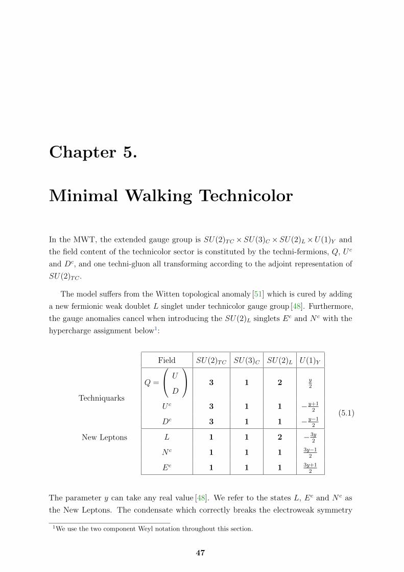
In the MWT, the extended gauge group is SU(2)TC ×SU(3)C ×SU(2)L×U(1)Y and
the field content of the technicolor sector is constituted by the techni-fermions, Q, U c
and Dc, and one techni-gluon all transforming according to the adjoint representation of
SU(2)TC .
The model suffers from the Witten topological anomaly [51] which is cured by adding
a new fermionic weak doublet L singlet under technicolor gauge group [48]. Furthermore,
the gauge anomalies cancel when introducing the SU(2)L singlets Ec and N c with the
hypercharge assignment below1:
Techniquarks
New Leptons
Field SU(2)TC SU(3)C SU(2)L U(1)Y
Q =
U
D
3 1 2 y2
U c 3 1 1 −y+12
Dc 3 1 1 −y−12
L 1 1 2 −3y2
N c 1 1 1 3y−12
Ec 1 1 1 3y+12
(5.1)
The parameter y can take any real value [48]. We refer to the states L, Ec and N c as
the New Leptons. The condensate which correctly breaks the electroweak symmetry
1We use the two component Weyl notation throughout this section.
47

48 Minimal Walking Technicolor
is 〈UU c +DDc〉. To discuss the symmetry properties of the theory it is convenient to
arrange the technifermions as a column vector, transforming according to the fundamental
representation of SU(4)
Q =
U
D
U c
Dc
, (5.2)
The breaking of SU(4) to SO(4) is driven by the following condensate
〈QTEQ〉 (5.3)
The matrix E is a 4× 4 matrix defined in terms of the 2-dimensional unit matrix as
E =
0 1
1 0
. (5.4)
The above condensate is invariant under an SO(4) symmetry.
5.1. Goldstone Bosons
5.1.1. Effective Theory
The symmetry breaking pattern of the MWT model is SU(4)→SO(4). This leaves us
with nine broken generators with associated Goldstone bosons. As in Section 3.1 ,the
resulting low energy effective theory can be organized in a derivative expansion with
cut-off scale 4πF , where F is the Goldstone boson decay constant. We first introduce
the matrix:
U = exp
(i
√2
FΠaXa
)E , (5.5)

Minimal Walking Technicolor 49
where Πa are the 9 Goldstone bosons and Xa are the 9 broken generators ( see Appendix
of [I]). The matrix U transforms under SU(4) in the following way:
U → gUgT , g ∈ SU(4). (5.6)
The leading term appearing in the Lagrangian is:
LU =F 2
2Tr[DµUD
µU †]. (5.7)
The electroweak covariant derivative reads:
DµU = ∂µU − i[GµU + UGT
µ
](5.8)
where
Gµ = g2 Waµ L
a + g1 Bµ
(−R3T +
√2 y S4
). (5.9)
Here g1 and g2 are the hypercharge and the weak couplings, respectively. The value of F
is fixed in order to reproduce correctly the electroweak symmetry breaking F = 2mWg2
.
The gauging of the electroweak interactions breaks explicitly the SU(4) symmetry
group down to SU(2)L×U(1)Y ×U(1)V , while the spontaneous symmetry breaking
leaves invariant an SO(4) subgroup. The remaining unbroken group is U(1)Q×U(1)V .
The U(1)Q factor is the symmetry group associated to the electromagnetism while the
U(1)V leads to the conservation of the technibarion number. A simple illustration of the
spontaneous and explicit breaking of the SU(4) symmetry is presented in Figure 5.1.
Among the 9 physical degrees of freedom, 3 are eaten up by the longitudinal components
Particle Physics & Origin of Mass
CP - Origins3
where
Gµ = g Waµ La + g� Bµ
�−R3T
+√
2 y S4�. (10)
The gauging of the electroweak interacations breaks explicitly the SU(4) symmetry
group down to SU(2)L ×U(1)Y ×U(1)V, while the spontaneous symmetry breaking leaves
invariant an SO(4) subgroup. The remaining unbroken group is U(1)Q×U(1)V. The U(1)Q
factor is the symmetry group associated to the electromagnetism while the U(1)V leads to
the conservation of the technibarion number.
Among the 9 physical degrees of freedom, 3 are eaten up by the longitudinal compo-
nents of the SM gauge boson while the remaining 6 Goldstone bosons carry technibaryon
number and will be denoted by ΠUU,ΠUD and ΠDD (for a detailed classification of these
state see the Appendix A).
These states acquire a mass because of the gauging of the SM subgroup in SU(4). An
explicit calculation of the mass splitting leads to [28]
∆m2ΠUU=
m2walk
g21 + g2
2
�g2
1(1 + 2y)2 + g22
�(11)
∆m2ΠDD=
m2walk
g21 + g2
2
�g2
1(4y2 − 1) + g22
�(12)
∆m2ΠUD=
m2walk
g21 + g2
2
�g2
1(1 − 2y)2 + g22
�. (13)
Here g1 and g2 are the hypercharge and the weak couplings respectively. With walking
dynamics the value of mwalk can be even of few hundreds GeV [28].
However, in order to be sure to obtain a phenomenological viable spectrum, it is
possible to introduce an extra source of symmetry breaking. A common ETC mass for all
the uneaten PNGBs can be provided by adding the following term to (8)
−m2etcF
2
4Tr�U†BVUBV
�(14)
with
BV =
0
0 −
. (15)
Note that this mass term is not linear in U as is the mass term for the pions in QCD. This
is so since it is expected to come from a four-techniquark interaction term, furthermore
7
Figure 5.1.: Spontaneous and explicit breaking of the SU(4) symmetry.

50 Minimal Walking Technicolor
of the SM gauge bosons while the remaining 6 Goldstone bosons carry technibaryon
number and will be denoted by ΠUU ,ΠUD and ΠDD. Because Goldstone bosons carry
technibaryon number, we refer to these states also as technibaryons.
The bosons can be classified according to the unbroken group U(1)V ×U(1)Q in the
following way:
Boson U(1)V charge U(1)Q charge Linear Combination
W+L 0 +1 Π1−iΠ2
√2
W−L 0 −1 Π1+iΠ2
√2
ZL 0 0 Π3
ΠUU +1 y − 1 Π4+iΠ4+Π6+iΠ7
2
ΠDD +1 y + 1 Π4+iΠ4+Π6+iΠ7
2
ΠUD +1 y Π8+iΠ9√
2
Π†UU −1 −y + 1 Π4−iΠ4+Π6−iΠ7
2
Π†DD −1 −y − 1 Π4−iΠ4+Π6−iΠ7
2
Π†UD −1 −y Π8−iΠ9√
2
(5.10)
Electroweak interactions split the technipion masses according to the following pat-
tern [52]:
∆m2ΠUU
=m2
walk
g21 + g2
2
[g2
1(1 + 2y)2 + g22
](5.11)
∆m2ΠDD
=m2
walk
g21 + g2
2
[g2
1(4y2 − 1) + g22
](5.12)
∆m2ΠUD
=m2
walk
g21 + g2
2
[g2
1(1− 2y)2 + g22
]. (5.13)
In models with walking dynamics the value of mwalk can be even of few hundreds GeV[52].
Furthermore it is also possible to introduce a common mass term for the pseudo Goldstone
bosons by adding the following term to the Lagrangian (5.7):
− m2etcF
2
4Tr[U †BVUBV
](5.14)

Minimal Walking Technicolor 51
with
BV =
1 0
0 −1
. (5.15)
This term was already added in [53] and it is expected to emerge from a more complete
theory of SM fermion mass generation. It is expected to emerge from a four-techniquark
interaction term, and preserves SU(2)L×SU(2)R×U(1)V of SU(4), which contains the
SU(2)V custodial symmetry group.
It is useful to know the transformation properties of the matrix U with respect to
the electroweak gauge group. Under SU(4) the matrix U transforms as a two index
symmetric tensor, or in other words U transforms like the irreducible representation 10
of SU(4):
U → gUgT , g ∈ SU(4). (5.16)
Knowing the embedding of the electroweak generators in the SU(4) algebra it is possible
to decompose the representation 10 according to the SU(2)L×U(1)Y group:
10 → 3y + 21/2 + 2−1/2 + 1−y+1 + 1−y + 1−y−1 . (5.17)
The identification of these representations inside the U matrix is given by:
3y → TL
21/2 → H2
2−1/2 → H1
1−y−1 → S1
1−y → S2
1−y+1 → S3
U =1
F
TL H1√
2H2√
2
HT1√2
HT2√2
S1S2√
2
S2√2
S3
(5.18)
By expanding the exponential in equation (5.5) to the second order in the number
pseudo Goldstone boson fields, we identify the following phenomenologically relevant

52 Minimal Walking Technicolor
interaction Lagrangian for the first LHC searches:
TL = i
ΠUUΠUD√
2
ΠUD√2
ΠDD
S1 = iІUU S2 = iІUD S3 = iІDD (5.19)
H1√2F
=
1− Π†UDΠUD+2 Π†UUΠUU4F 2
−Π†UDΠDD+Π†UUΠUD
2√
2F 2
H2√2F
=
−Π†DDΠUD+Π†UDΠUU
2√
2F 2
1− Π†UDΠUD+2 Π†DDΠDD4F 2
. (5.20)
Depending on the specific choice of the hypercharge assignment y, one can construct
different Yukawa-type interactions involving the matrix U . Odd integer values are
required for y to avoid stable composite states with fractional electric charge2. In general,
electrically charge stable states are excluded by cosmology, see for example discussion
in [54].
Within this setup the allowed Yukawa terms are
L2HDM = H2quc +H1qd
c +H1lec +H2LN
c +H1LEc (5.21)
+ Hc1qu
c +Hc2qd
c +Hc2le
c +Hc1LN
c +Hc2LE
c + h.c.
LΠψψ =
y = −3 S†3ecec + h.c.
y = −1 S†1ecec + S2ll + T †Lll + h.c.
y = +1 S3ecec + S†2ll + TLll + h.c.
y = +3 S1ecec + h.c.
(5.22)
LΠLL =
y = −1 S1EcEc + h.c.
y = +1 S3NcN c + h.c.
(5.23)
LΠLψ =
y = −5 S1Ecec + h.c.
y = −3 S†1Ll + S1Ncec + S2E
cec + h.c.
y = −1 S†2Ll + S2Ncec + T †LLl + h.c.
y = +1 Hc1Le
c +H2Lec +H1N
cl +Hc2N
cl + S3Ll + S3Ncec + h.c.
(5.24)
Hci is defined as Hc
i ≡ −iσ2H∗i , and the ec and l symbols stand respectively for SU(2)L
singlet and doublets states of the 3 lepton families (e, µ, τ). In equations (5.21)-(5.24),
2Bound states made by one technifermion and one technigluon have electric charge −y± 12

Minimal Walking Technicolor 53
for simplicity, we omitted the appropriate SU(2)L contractions, the flavor indices and
the coupling constants in front of each term. The interactions in (5.21)-(5.24) are valid
for generic ETC models. Specific models can provide further symmetries which can
be exploited to reduce the number of operators in (5.21)-(5.24). Moreover, it is worth
noticing that quarks can couple, to this order, only to the Higgs sector (via L2HDM ), i.e.
quadratic in the number of technipions.
5.1.2. Results
The allowed values for y can be further restricted by requiring that the lightest state,
among the pseudo Goldstone bosons and the new leptons, is not electrically charged and
stable. According to this, we discard the cases y = {−5, 3} and the surviving values of y
are {−3,−1, 1}.
For every y, the neatest process to be investigated at the LHC involving the PGBs
for which we will derive relevant constraints is
pp→Π†2Π2→ (`−i `−j )(`+
h `+k ) where i, j, h, k = e, µ, τ. (5.25)
The flavor structure of the coupling λijΠ2l+i l
+j depends on the ETC sector, but given
that this sector is unknown it is possible to have different lepton pairs in the final state.
In order to simplify our analysis, we assume decays only into a pair of same sign muons.
The ATLAS collaboration has studied the production of a doubly charged Higgs boson
at the LHC in [55] with 1.6 fb−1 of integrated luminosity. This study was performed
by examining the invariant mass distribution of the same sign muon pairs. The doubly
charged particle is assumed to decay into two muons with 100% branching fraction.
We have used the number of observed events and the number of expected background
events reported in table 2 of [55] to calculate the 95% exclusion limit for the pseudo
Goldstone boson production using the modified frequentists CLs method [56,57]. The
value for the coupling between the pseudo Goldstone boson and the muons is chosen
according to [55], to ensure that the pseudo Goldstone bosons are decaying before the
detector. This yields a lower limit of 286 GeV for the pseudo Goldstone boson mass.
The exclusion plot is presented in Figure 5.2 for 1.6 fb−1.

54 Minimal Walking Technicolor
mass (GeV)±±W150 200 250 300 350 400
) (fb
)-µ
2+µ
2A
±±
W ±±
W A
(pp
m
1
10
210
)-µ 2+µ 2A ±±W ±±W A(pp m
-1 L dt = 1.6 fb095% upper limit, ATLAS data,
-1 L dt = 5 fb095% expected limit,
-1 L dt = 15 fb095% expected limit,
| < 2.5d > 20 GeV, |pp @ 7 TeV, y = -1, p
W) < 1.1 m±µ±µ < m(W0.9 m
Figure 5.2.: Exclusion for a doubly charged PGB with y = −1 based on the ATLAS data.
5.1.3. Summary
This sector of the Minimal Walking Technicolor model was for the first time investigated in
[I]. Strongly coupled theories are in many occasions studied in terms of vector resonances.
Nevertheless, it is possible that pseudo Goldstone bosons are the the first sign of strong
dynamics at the LHC.
The signature which is identified to be the most important can also arise from many
theories with doubly charged Higgs bosons. Usually in these models, producing a single
doubly charged Higgs is more economical. If doubly charged scalar states are observed
to be produced only in pairs, this would favor our model. Of course the reverse is true as
well.
5.2. Vector Resonances
Different walking technicolor models posses different global symmetries and symmetry
breaking patterns. The precision measurements dictates that all these different extension
of the SM have to contain at least the following chiral symmetry breaking pattern:
SU(2)L×SU(2)R→SU(2)V . (5.26)

Minimal Walking Technicolor 55
Thus the NMWT model serves as a template to study vector resonance phenomenology
at the LHC. Based on the symmetry breaking pattern, the low energy spectrum is
described in terms of lightest spin one vector and axial-vector iso-triplets V ± ,0 and A± ,0
as well as lightest iso-singlet scalar resonance H. The corresponding states in the QCD
are the ρ± ,0, a± ,01 and the f0(600).
All the results in paper [II] are obtained using a linearly realized effective Lagrangian.
How to write down this effective Lagrangian is described in details in [53,58]. Out of
author’s own interest, let us write down a non-linear effective Lagrangian, supplemented
with a scalar singlet state (i.e. the Higgs), and compare it with the Linear realization.
5.2.1. Non-linear Lagrangian
In order to consistently introduce mass terms for the vector mesons the Generalized
Hidden Local Symmetry (GHLS) method is employed [59]. Formalism is based on the
observation that a nonlinear sigma model based the manifold G/H is gauge equivalent
to a linear model with symmetry group GGlobal×Glocal. The vector mesons are taken to
be gauge bosons of the Glocal symmetry and a subgroup of GGlobal is gauged under the
electroweak interactions. The gauge equivalence is straightforward to verify by using the
equations of motion of the gauge bosons and choosing a special gauge for the local group.
In our case GGlobal = SU(2)L×SU(2)R and Glocal = SU(2)L×SU(2)R. A basic
dynamical variable of the GGlobal×Glocal model is a unitary matrix field U(x) [59–61]
transforming as
U(x)→U(x′) = h(x)U(x)g†, (5.27)
where h(x) ∈ Glocal and g ∈ GGlobal. It is convenient to decompose the U(x) as
U(x) = ξ†L(x)ξM(x)ξR(x) (5.28)
The variables ξ(x) transform as
ξL(R)→hL(R)(x)ξL(R)(x)g†L(R), ξM→hL(x)ξM(x)h†R(x), (5.29)

56 Minimal Walking Technicolor
where gL(R) ∈[SU(2)L(R)
]Global
and hL(R) ∈[SU(2)L(R)
]Local
. We can construct the
Lagrangian by introducing the covariant Maurer-Cartan 1-forms defined as:
αµL,R,M(x) = DµξL,R,M(x) · ξ†L,R,M(x). (5.30)
The covariant derivatives for the different ξ fields are given as
DµξL(x) = ∂µξL(x)− iLµ(x)ξL(x) + iξL(x)Lµ(x) (5.31)
DµξR(x) = ∂µξR(x)− iLµ(x)ξR(x) + iξR(x)Rµ(x) (5.32)
DµξM(x) = ∂µξM(x)− iLµ(x)ξM(x) + iξM(x)Rµ(x), (5.33)
where Lµ = gW aµT
a and Rµ = g′BµT3 are the ordinary electroweak gauge bosons
introduced by gauging the SU(2)L×U(1)Y subgroup of GGlobal symmetry. The GLocal
gauge bosons are defined to include the gauge coupling g
Lµ = gVµ − Aµ√
2, Rµ = g
Vµ + Aµ√2
. (5.34)
Finally the Lagrangian is
L = Lkin + aLV + bLA + cLM + dLπ, (5.35)
where
Lkin = −1
2Tr [WµνWµν ]−
1
4BµνBµν −
1
2Tr [VµνVµν + AµνAµν ] , (5.36)
LV = F 2Tr[α‖µα‖µ
], LA = F2Tr [α⊥µα
µ⊥] , LM = F2Tr [αMµα
µM] , (5.37)
Lπ = F 2Tr [(α⊥µ + αMµ)(αµ⊥ + αµM)] . (5.38)
The perpendicular and parallel projections are defined as
αµ‖,⊥ = (ξM αµRξ†M ± α
µL)/2. (5.39)

Minimal Walking Technicolor 57
And the field strengths are
Wµν = ∂µWν − ∂νWµ − ig [Wµ,Wν ] , (5.40)
Bµν = ∂µBν − ∂νBµ, (5.41)
Vµν = ∂µVν − ∂νVµ − ig [Vµ, Vν ] , (5.42)
Aµν = ∂µAν − ∂νAµ − ig [Aµ, Aν ] . (5.43)
The Lagrangian (5.35) can be extended to include states which are singlets under the
stability group H. After adding a scalar state the Lagrangian reads
L = Lkin + ka(χ)aLV + kb(χ)bLA + kc(χ)cLM + kd(χ)dLπ
+ kh(χ)1
2∂µh∂
µh− V(χ),(5.44)
where χ = h/v and v is an arbitrary scale. The arbitrary functions kx(χ) must satisfy
ka(0) = kb(0) = kc(0) = ka(0) = kh(0) = 1 (5.45)
for a proper normalization of the Goldstone boson kinetic terms. The function kd(χ)
stands in front of a mixed term and the former requirement does not apply. Nevertheless,
we will choose it to satisfy the same condition. One can derive the interactions with h
expanding kx(χ) around χ = 0.
5.2.2. Linear Lagrangian
Let us write down the linearly realized effective Lagrangian for comparison:
Lboson = −1
2Tr[WµνW
µν]− 1
4BµνB
µν − 1
2Tr [FLµνF
µνL + FRµνF
µνR ]
+ m2 Tr[C2
Lµ + C2Rµ
]+
1
2Tr[DµMDµM †]− g2 r2 Tr
[CLµMCµ
RM†]
− i g r3
4Tr[CLµ
(MDµM † −DµMM †)+ CRµ
(M †DµM −DµM †M
)]+
g2s
4Tr[C2
Lµ + C2Rµ
]Tr[MM †]+
µ2
2Tr[MM †]− λ
4Tr[MM †]2 (5.46)
where Wµν and Bµν are the ordinary electroweak field strength tensors, FL/Rµν are the
field strength tensors associated to the vector meson fields AL/Rµ, and the CLµ and CRµ

58 Minimal Walking Technicolor
fields are
CLµ ≡ ALµ −g
gWµ , CRµ ≡ ARµ −
g′
gBµ . (5.47)
The 2× 2 matrix M is
M =1√2
[v +H + 2 i πa T a] , a = 1, 2, 3 (5.48)
where πa are the Goldstone bosons produced in the chiral symmetry breaking, v = µ/√λ
is the corresponding VEV, H is the composite Higgs, and T a = σa/2, where σa are the
Pauli matrices. The covariant derivative is
DµM = ∂µM − i g W aµ T
aM + i g′ M Bµ T3 . (5.49)
When M acquires its VEV, the Lagrangian of equation (5.46) contains mass mixing
terms for the spin-1 fields.
5.2.3. Comparison
The new vector resonances mass mixes with the SM gauge bosons. This induces the
couplings between the new vectors and the SM fields. The masses depend on the
parameters a, b, c, d in the nonlinear model and on the parameters r1, r2, r3, k in the
linear model. This in addition to a parameter fixing the scale and the gauge couplings.
If we are interested in signatures at the LHC not involving the Higgs, it seems that at
leading order we can define a mapping between the parameters of these two realizations
of the model.
In the linear Lagrangian the symmetry SU(2)L×SU(2)R fixes the Higgs couplings to
be given in terms of parameters a, b, c, d. In the non-linear realization all the couplings
involve independent free parameters. The couplings between the new vector states and
the Higgs are important when we calculate decay widths for the vector resonances. This
can, without a doubt, have an effect on the results, even if we study processes without
the Higgs. In Figure 5.3 we have plotted the decay width of the R1 vector resonance in
the linear model and in the non-linear model taking kx(χ) = 0. Notice here that the
discussion applies to any theory with the same global symmetry. Connection to the
underlying gauge theory can be achieved via the WSRs, which impose relations between
the parameters. In rest of the chapter we will use the Linear Lagrangian.

Minimal Walking Technicolor 59
500 1000 1500 2000
0.1
0.5
1.0
5.0
10.0
50.0
MA
Wid
th@G
eVD
R1 -> 2 X
Linear
Non-linear
Figure 5.3.: The decay width of the R1 vector resonance.
5.2.4. Results
As already mentioned, the new vector and axial-vector states mix with the SM gauge
eigenstates yielding the ordinary SM bosons and two triplets of heavy mesons, R± ,01 and
R± ,02 , as mass eigenstates. The couplings of the heavy mesons to the SM particles are
induced by the mixing. Important here is how the heavy vectors couple to the fermions.
In the region of parameter space where R1 is mainly an axial-vector and R2 mainly a
vector sate, the dependence of the couplings to the SM fermions as a function of g is
very roughly
gR1,2ff ∼g2
g(5.50)
where g is the electroweak gauge coupling. The full coupling constant is also a function
of MA, but this dependence is very weak.
To constrain the parameter space of the model we use the CMS results [62], which
report limits for a W ′ boson decaying to a muon and a neutrino at√s = 7 TeV in the
mass range 600 - 2000 GeV for the resonance.
The relevant calculations are performed using MadGraph [63], using the CTEQ6L
parton distribution functions [64], and the implementation for the NMWT model [65].
reference [62] reports experimental limits for the muon channel together with a combined
analysis with the electron channel [66]. Because of the missing energy in the final state,
the invariant mass of the resonance cannot be reconstructed, and the following transverse

60 Minimal Walking Technicolor
Tevatron
Consistency of the theory
YW
CMS Data �1�5 fb�1, 3 Σ5 fb�1, 5 Σ13 TeV, 100 fb�1, 3 Σ13 TeV, 100 fb�1, 5 Σ
0.5 1.0 1.5 2.0 2.5
2
4
6
8
10
12
MA �TeV�
g�
Walking
Running
Figure 5.4.: Bounds in the (MA, g) plane of the NMWT parameter space: (i) CDF directsearches of the neutral spin one resonance excludes the uniformly shaded areain the left, with MH = 200 GeV and s = 0. (ii) The 95 % confidence levelmeasurement of the electroweak precision parameters W and Y excludes thestriped area in the left corner. (iii) Imposing the modified WRS’s excludes theuniformly shaded area in the right corner. (iv) The horizontal stripe is excludedimposing reality of the axial and axial-vector decay constants. (v) The area belowthe thick uniform line is excluded by the CMS data [62]. (vi) Dashed and dottedlines are expected exclusions using different values of the integrated luminosityand center of mass energy.
mass variable is utilized
MT =√
2 · pTEmissT · (1− cos ∆φµ,ν). (5.51)
In the experimental analysis, the cut on the transverse mass is adjusted in bins of the
mass of the sought-after resonance. In addition to the transverse mass cut, the lepton
acceptance |η| < 2.1 is used. The resulting cross section is then compared with the limits
reported in the experimental analyses.
Exploring the signal from the process pp→R1,2→ lν we are able to limit the possible
values for the parameters MA and g. The theoretical limits as well as the limits from the
Tevatron are described in [67]. The MA, g plane of the parameter space is presented in
Figure 5.4 for MH = 200GeV and s = 0.

Minimal Walking Technicolor 61
The uniformly shaded region on the left is excluded by the CDF searches of the
resonance in the the pp→ e+e− process. The striped region in the lower left corner is
excluded by the measurements of the electroweak W and Y parameters [68] adapted
for models of MWT in [69]. Avoiding imaginary decay constants for the vector and
axial-vector sets an upper bound for the g, i.e. excludes the uniformly shaded in the
upper part of the figure. The near conformal (walking) dynamics modifies the WRS’s,
compared to a running case like QCD, as explained above [70]. Imposing these modified
sum rules excludes the lower right corner of the parameter space. The CDF exclusion
limit is sensitive, indirectly, to the mass of the composite Higgs and the coupling s via
properties of the new heavy spin one states. However, the edge of the excluded area
varies only very weakly as a function of s and MH . The CMS search imposes a 95 % CL
exclusion bound described with the thick solid (red) line. The thick dashed and dotted
lines (blue) are three and five sigma exclusion limits for 7 TeV and 5 fb−1. The thin
dotted and dashed lines describe the reach of the LHC with 100 fb−1 at 13 TeV. The three
and five sigma exclusion limits are calculated using poisson distribution, following [71].
Due to the effective description, we have not employed the K-factors when calculating
the exclusion limits.
Comparing the three sets of lines for the LHC, the increase in the horizontal direction
follows roughly the increase in luminosity. The small role of the center of mass energy
can be understood by exploring the behavior of the cross section as a function of the
center of mass energy and comparing it with the scaling with g, obtained from equation
(5.50).
5.2.5. Summary
The limits on the masses are significantly lower that for the W ′ with SM like couplings.
The reason for this can be traced back to fermion couplings which arise via mixing. The
ATLAS Collaboration has performed a similar analysis with this model and reported
results in [72]. The exclusion plot derived by ATLAS is shown in Figure 5.5
As evidenced in Figure 5.5, the leptonic final states are not enough to explore the
whole parameter space. Interesting possibility is to use associate Higgs production to find
vector resonances. For example, in the process pp→R1→ZH the new vector state has
only one coupling with the fermions which will help with large values of g. An example
invariant mass distribution is given in Figure 5.6. Here the Higgs is taken to decay to

62 Minimal Walking Technicolor
Figure 5.5.: Excluded parameter space based on the ATLAS measurements. The plot is takenfrom [72]
) (GeV)-l+lbM(b
400 500 600 700 800 900 1000 1100
/dM
(fb
/10
GeV
)σd
-410
-310
-210
-110
1
=5, S=0.3g~=700 GeV, AM
=125 GeVh
sm, m
=702 GeVR1M
=1055 GeVR2M
> 25GeV2,b
> 45GeV, p1,b
| < 4.5, pb
|y
> 20GeVl
| < 2.5, pl
|y
) < 135 GeVb)>0.7, 110 GeV < M(b,bR(b,∆
= 8TeVspp @
)-l+ l→Z, (Z b b→pp
Figure 5.6.: Production cross section as a function of invariant mass MHZ .

Minimal Walking Technicolor 63
b-quark pair and the Z boson to leptons. To effectively use this channel requires a great
deal of integrated luminosity and efficient b-tagging.
5.3. Technicolor Higgs
In technicolor the Higgs sector is replaced with a strongly interacting sector. The lightest
scalar state plays a role of the Higgs bosons, provided that it is lighter compared to other
sates. In QCD like models, mass of the composite Higgs is estimated to be roughly of the
order of MH ∼ 1 TeV, which is of course way too heavy when compared to the observed
Higgs mass. In walking models the mass of the Higgs can be as low as few hundreds of
GeV [48,73]. In order to explain why one scalar state if much lighter than other states
the model, it is convenient to identify it with the Goldstone boson of the approximate
scale symmetry. This scenario goes under the name techni-dilation [74].
What we have stated is not quite the complete picture. The Higgs here is composed
of massless techniquarks and all the mass is given by the dynamics. The dynamical mass
is not the physical mass; one has to consider also the effect from the radiative corrections.
The SM top-induced radiative corrections can reduce the composite Higgs mass down
to observed value [73]. This is like an inverse of the little hierarchy problem causing
problems in several BSM models.
5.3.1. Hybrid Model
Inspired by the hybrid models used to calculate the two photon decay of the sigma meson
in QCD, we calculated in [I] the effect of techniqurks on the Higgs two photon decay. The
contribution to the process is modeled by re-coupling, in a minimal way, the composite
Higgs to the techniquarks Q via the following operator:
LTC−2γ =√
2MQ
vweak
[QL
t ·HDRt +QL
t · (i τ2H∗)URt
]+ h.c. , (5.52)
where MQ is the dynamical mass of the techniquark and t = 1, . . . , d[r] is the Technicolor
index and d[r] the dimension of the representation under which the techniquarks transform.
If the model suffers from the Witten anomaly, a lepton family is added
LL−2γ =√
2ME
vweakLL ·HER +
√2MN
vweakLL · (i τ2H
∗)NR + h.c. , (5.53)

64 Minimal Walking Technicolor
where ME and MN are the fermion masses. The techniquark dynamical mass is intrinsi-
cally linked to the technipion decay constant Fπ via the Pagels-Stokar formula [75,76]
MQ ≈ 2πFπ√d(r)
.
The one loop Higgs decay width to two photons for any weakly interacting elementary
particle contributing to this process can be neatly summarized as [77]:
Γ(h→ γγ) =α2GFM
2h
128√
2π3
∣∣∣∣∣∑i
ni Q2i Fi
∣∣∣∣∣2
, (5.54)
where i runs over the spins, ni is the multiplicity of each species with electric charge Qi
in units of e. The Fi functions are given by
F1 =2 + 3τ + 3τ(2− τ)f(τ), (5.55)
F1/2 =− 2τ [1 + (1− τ)f(τ)], (5.56)
F0 =τ (1− τf(τ)) , (5.57)
where τ =4m2
i
M2h
and
f(τ) =
(
arcsin√
1τ
)2
, if τ ≥ 1
−14
(log(
1+√
1−τ1−√
1−τ
)− iπ
)2
, if τ < 1. (5.58)
The lower index of the function F represent the spin of each particle contributing in the
process.
5.3.2. Results
We plot in Figure 5.7 the intrinsic dependence on the dimension of the Technicolor matter
representation d[r] according to the ratio:
R =ΓSM(h→ γγ)− ΓTC(h→ γγ)
ΓSM(h→ γγ). (5.59)
For any odd representation we included the Lepton contribution and therefore we could
not simply join the points. Interestingly when d[r] is around 7 the contribution from the
techniquarks and from the SM fermions (mainly the top) cancels the W contribution
leading to ΓTC ≈ 0.
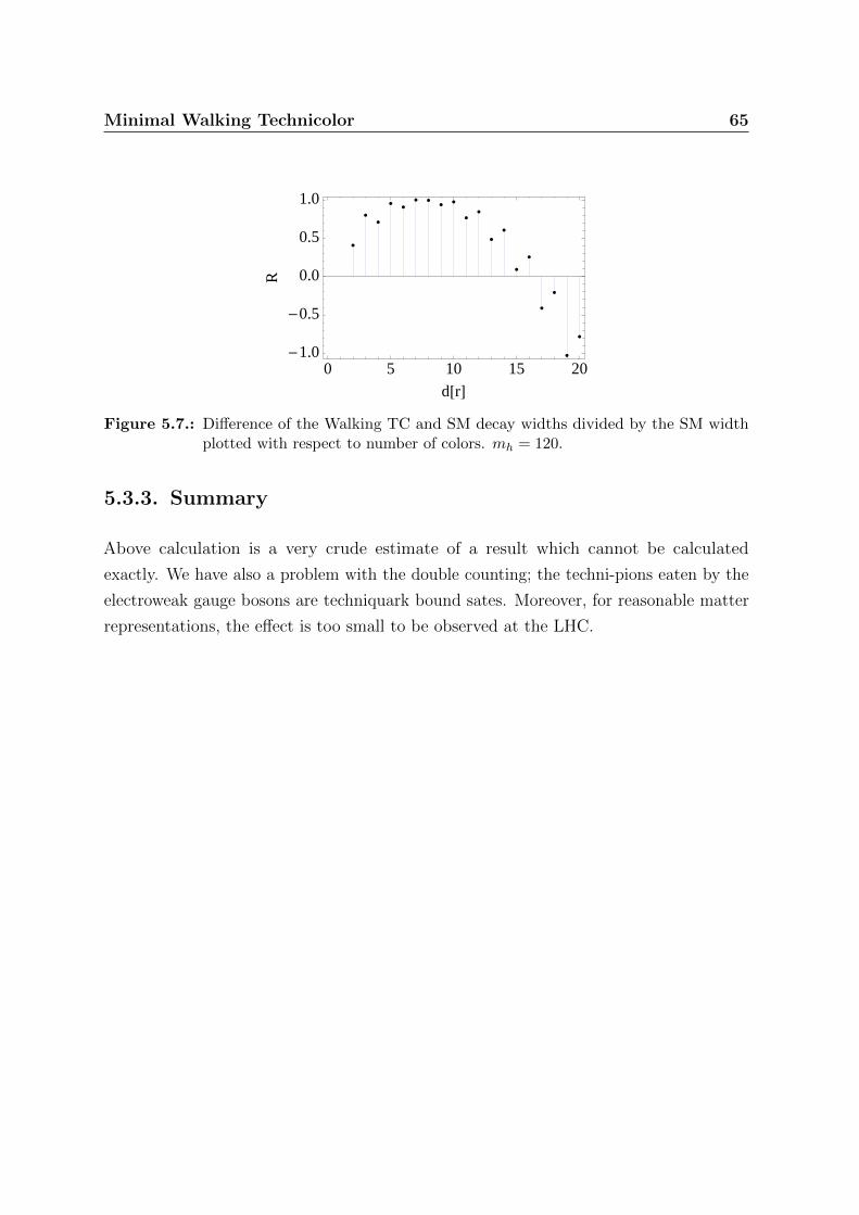
Minimal Walking Technicolor 65
0 5 10 15 20-1.0
-0.5
0.0
0.5
1.0
d@rD
R
Figure 5.7.: Difference of the Walking TC and SM decay widths divided by the SM widthplotted with respect to number of colors. mh = 120.
5.3.3. Summary
Above calculation is a very crude estimate of a result which cannot be calculated
exactly. We have also a problem with the double counting; the techni-pions eaten by the
electroweak gauge bosons are techniquark bound sates. Moreover, for reasonable matter
representations, the effect is too small to be observed at the LHC.

66

Chapter 6.
Dark Matter Model Building
Let us forget the problems with the SM Higgs sector for the rest of the thesis. A large
number of observational evidences suggest that there is non-luminous matter in the
universe [78]. This dark matter cannot be explained by the particles we know, thus
requires physics beyond the SM. There are a number of experiments around the world
which are trying to detect dark matter directly. The situation with these experiments
is quite interesting because they do not mutually agree; for example DAMA/LIBRA
[79], GoGeNT [80] and CRESST [81] claims to have seen dark matter while CDMS
[82], XENON [83] and PICASSO [84] experiments exclude the parameter regions where
observations have been made. However, there are number of caveats that need to be
discussed as one tries to interpret these results as discussed for example in [85].
6.1. The model
Effect of a magnetic dipole moment of the dark matter on the direct detection experiments
has been discussed in[85,86] using effective operator approach. In in [IV] we have provided
a renormalizable model which can, at low energies, provide this effective operator. On
top of the SM we add a vector-like heavy electron (E), a complex scalar (S) and a SM
singlet Dirac fermion (χ). The associated renormalizable Lagrangian is
LSEχy = LSM + χi/∂χ−mχχχ+ Ei /DE −mEEE − (SEχy + h.c.)
+ DµS†DµS −m2
SS†S − λHSH†HS†S − λS(SS†)2 , (6.1)
where Dµ = ∂µ− ie swcwZµ + ieAµ, sw and cw represent the sine and cosine of the Weinberg
angle. We assume the new couplings y, λHS and λS to be real and the bare mass squared
67

68 Dark Matter Model Building
of the S field to be positive so that the electroweak symmetry breaks via the SM Higgs
doublet (H). The interactions among χ, our potential dark matter candidate, and the
SM fields occur via loop-induced processes involving the SEχy operator in (6.1).
These extra interactions have an effect on the vacuum stability we investigated in
the introduction. However, the effect is very small because the scalar S does not acquire
a vacuum expectation value, as argued in [87]. Both of the new fermions can mix with
the SM leptons. For the sake of simplicity, we do not consider the effect of the mixing,
even though it can lead to interesting consequences. For example, sizable mixing can
explain the discrepancy between the measured and calculated muon anomalous magnetic
moment.
At the one loop level χ develops the following magnetic-type interactions
L5 =λχ2χσµνχF
µν − sw2 cw
λχχσµνχZµν , (6.2)
where F µν and Zµν are the photon and Z field strength tensors, and λχ is related to the
electromagnetic form factor F2(q2) as follows:
λχ =F2(q2)
2mχ
e . (6.3)
The explicit derivation of the one-loop–induced form factor can be found in the first
appendix of [IV]. It is enlightening to report the analytic form for a few interesting limits
to learn about the dependence upon couplings and masses. We start by considering the
static limit F2(0), useful for dark matter direct detection experiments. To reduce the
parameter space we take the masses of E and S to be degenerate mE = mS = M leading
to the simplified expression
F2(0) =y2
8π2
(2
z
√2 + z
2− ztan−1
(z√
4− z2
)− 1
), (6.4)
where z = mχM
. For small z we have
F2(0) =y2
16π2
(z +
z2
3
)+O
(z3), (6.5)
which for z = 0 gives λχ = ey2/(32π2M). It is also interesting to consider a dark matter
candidate with mass of the order of the electroweak scale or slightly higher. For this
purpose a simple estimate for the electromagnetic form factor can be deduced by setting

Dark Matter Model Building 69
z = 1 (i.e. mχ = M), and M around the electroweak scale, yielding F2(0) = y2
√3π − 3
24π2
and therefore λχ = ey2
√3π − 3
48π2M. From the two limits it follows that the scale of the
magnetic moment is controlled by the common mass of the heavy states M .
6.2. Results
It was shown in [85] that there is a region of parameter space able to alleviate the
tension between the experiments when using magnetic moment interactions. It was
observed that one can, in fact, bring DAMA, CoGeNT and CRESST signals to overlap
while being marginally consistent with CDMS, XENON and PICASSO experiments
(see Fig. 3 of ref. [85]). A best fit result leads to a dark matter mass around 10 GeV
and a constant magnetic moment of about 1.5× 10⁻¹⁸ e cm, which corresponds to
32π2M/y2 = eλχ∼ 10 TeV. For example for M ≈ 500 GeV we find y ≈ π meaning that
the underlying dynamics of the model can be explored at the electroweak scale.
The contour plot of equal λχ in the (M ,y) plane is shown in Figure 6.1 together with
the exclusion regions obtained using the following information: The CMS constraints
on charged long-lived particles, The XENON100 results [83] after having taken into
consideration the threshold effects [85] and the Higgs to two gamma constraints.
400 600 800 1000 1200M [GeV]
2
4
6
8
10
y
λHS=√
4π mχ =10 GeV
2.0 ·10−19 e · cm 6.0 ·10
−19 e · cm
15.0·10
−19 e · cm
20.0 ·10−19 e · cm
40.0 ·10
−19 e · cm
90.0·10−19 e
· cmh→γγXENON
CMS
400 600 800 1000 1200M [GeV]
2
4
6
8
10
y
λHS=4π mχ =10 GeV
2.0 ·10−19 e · cm 6.0 ·10
−19 e · cm
15.0·10
−19 e · cm
20.0 ·10−19 e · cm
40.0 ·10
−19 e · cm
90.0·10−19 e
· cmh→γγXENON
CMS
Figure 6.1.: Strength of the magnetic moment λχ in the (M,y) plane with mχ = 10 GeV andfor λHS =
√4π (left panel) and λHS = 4π (right panel). The unshaded region is
the one allowed by experiments.

70 Dark Matter Model Building
6.3. Summary
The extension of the SM presented here can be tested at the LHC while providing a
dark matter candidate interacting with ordinary matter via magnetic operators which
can be simultaneously investigated or observed in dark matter experiments. In most
cases the link between the experiments can be established on within a renormalizable
model. Number of papers have been studying limits on the dark matter production at
the LHC using the same effective operators as for the direct detection. This can be, and
is, dangerous due to vastly different energy scales.

Appendix A.
Witten Anomaly
Let us consider an Euclidean SU(2) Yang-Mills theory in the compact space S4. Following
Witten, the global SU(2) anomaly is based on the observation that the fourth homotopy
group of SU(2)
Π4(SU(2)) = Z2 (A.1)
is nontrivial [51]. Homotopy groups are invariant under a homeomorphism, hence they
are topological invariants [88]. The homeomorphism classify spaces according to whether
can they be continuously deformed one to another. Thus homotopy groups offers a less
restrictive way to classify spaces since spaces that have same homotopy groups are not
necessarily homeomorphic. In physics homotopy groups are usually used to classify maps
rather than spaces.
The group manifold of the SU(2) is S3. Thus the gauge transformations are maps
U(x) : S4→S3. The equation (A.1) can be interpreted so that there exists different
types of gauge transformations which approach unity at infinity1. The fact that fourth
homotopy group is Z2 means that there is a topologically non-trivial gauge transformation
that cannot be smoothly deformed to the identity but when the transformation is done
twice it can be deformed to the identity.
Due to the topologically non-trivial mapping, for the every gauge field there is a
conjugate field
AUµ = U−1AµU − iU−1∂µU. (A.2)
1S4 is achieved from the R4 with the one-point compactification R4⋃{∞}. Thus the gauge transfor-
mations have to possess a constant value at the infty.
71

72 Witten Anomaly
And they both give exactly the same contribution to the functional integral
Z =
∫dψdψdAµ exp
(−∫d4x[
1
2g2tr(F 2) + ψi /Dψ]
), (A.3)
where ψ denotes a single left-handed fermion doublet. The Dirac operator i /D is hermitian,
thus the eigenvalues of the operator are real. Since the gamma matrices γµ and γ5
anticommute, for every eigenvalue λ there is an eigenvalue −λ
i /Dψ = λψ, i /D(γ5ψ) = −λ(γ5ψ). (A.4)
If the doublet ψ contains Weyl fermions, the integral over the fermion field is∫dψdψ exp
(−∫d4xψi /Dψ
)=√
det i /D, (A.5)
where the determinant is the product of eigenvalues [89]. The square root stands for the
product of the half of the eigenvalues.
We can choose that the square root of the eigenvalues is the product of positive
eigenvalues. The key point is that there exists a possibility for the positive and negative
eigenvalues to interchange their places under the non-trivial gauge transformation. One
possible eigenvalue flow is represented in the figure A.1. If the number of flows
interchanging positive and negative eigenvalue pairs is odd, it follows that
det i /D(A) = − det i /D(AU). (A.6)
The gauge fields Aµ and AUµ contribute equally to the functional integral (A.3), which
means that it vanishes in this case.
In order to show that this kind of eigenvalue flow happens, Witten defines an instanton-
like gauge field
At(τ)µ = (1− t(τ))Aµ + t(τ)AUµ , 0 ≥ t(τ) ≥ 1 (A.7)
and considers a five dimensional Dirac equation
/D(5)
Ψ =5∑i=1
γi
(∂i +
3∑a=1
Aai Ta
)Ψ = 0. (A.8)

Witten Anomaly 73
Figure A.1.: Eigenvalue flow under the non-trivial mpping.
The fifth component is the path parameter τ so that t(τ) = 1 when τ→ +∞ and t(τ) = 0
when τ→ −∞. Since Aa5 = 0 and the gamma matrices are real and symmetric we can
write the equation (A.8) as
dΨ
dτ= −γτ /D4
Ψ, (A.9)
where /D4
is a four dimensional Dirac operator for each τ . To solve this we write
Ψ(x, τ) = F (τ)φτ (x), (A.10)
where φτ (x) is the eigenfunction of the operator γτ /D4. In the adiabatic limit dφτ (x)
dτ= 0
and the equation (A.9) simpliffies to a form
dF (τ)
dτ= −λ(τ)F (τ). (A.11)
The solution to this equation is
F (τ) = F (0) exp
(−∫ τ
0
dxλ(x)
). (A.12)

74 Witten Anomaly
Now the logic goes as follows: According to mod 2 index theorem [90], the five-
dimensional Dirac operator has an odd number of zero eigenvalues. This impose that
equation (A.9) has an odd number of solutions. On the other hand equation (A.12)
is normalizable only if λ(τ) is positive for τ→ +∞ and negative for τ→ −∞. This
implies that there have to be odd number of eigenvalue pairs interchanging their places
confirming the equation (A.6) to hold in this case.
Vanishing path integral (A.3) causes a problem, because for each gauge invariant
operator the vacuum expectation value is
〈0|W |0〉 =
∫D[A, ψ, ψ] W e−S∫D[A, ψ, ψ] e−S
=”0”
0, (A.13)
which is not well defined. Thus the SU(2) gauge theory with odd number of Weyl fermion
doublets is inconsistent.
The hypothesis of adiabaticy is crucial in this derivation and criticism against this
point is represented in the reference [91]. However, there are also two other ways to state
the SU(2) anomaly. One is based on the U(1) anomaly and the rotation in the center of
the SU(2), which is free from perturbative anomalies [92]. In the third approach SU(2)
group is embedded into SU(3) group and the global anomaly result from the non-abelian
anomaly of the group SU(3) [93,94]. These alternative derivations confirm the existence
of the SU(2) anomaly.

Appendix B.
Dyson-Schwinger Equation
The Schwinger-Dyson equation is based on the simple observation the (functional) integral
of a (functional) derivative is zero [39]∫D[ψ]
δ
δψ≡ 0. (B.1)
This of course requires that the field ψ vanishes at spatial infinity. If we consider the
generating functional of a QCD like theory
Z [J, η, η] =
∫D[G,ψ, ψ
]eiS[G,ψ,ψ,J,η,η],
S[G,ψ, ψ, J, η, η
]=
∫d4x
[L+ JµG
µ + ¯etaψ + ψη],
(B.2)
where Jµ, η and η are the source fields, we have
0 =
∫D[G,ψ, ψ
] δS [G,ψ, ψ, J, η, η]δψiα(x)
eiS[G,ψ,ψ,J,η,η]. (B.3)
This can be written as[ηiα +
((i/∂ −mi)δ
αγ + gγµ(T a)αµ
δ
δiJaµ
)δ
δiηiγ
]Z [J, η, η] = 0. (B.4)
Differentiating with respect to ηjβ and dividing with Z give
δ4(x− y)δijδαγ + (i/∂x −mi)δ
αβ
i
Zδ2Z
δψiγ(x)δηjβ(y)
+gγµ(T a)αγ1
Zδ
δJaµ(x)
δ2Zδηiγ(x)δηjβ(y)
= 0,
(B.5)
75

76 Dyson-Schwinger Equation
which can be modified to a form
δ4(x− y)δijδαγ + (i/∂x −mi)δ
αβ i
(δ2 lnZ
δψiγ(x)δηjβ(y)+
δ lnZδηiγ(x)
δ lnZδηjβ(y)
)+gγµ(T a)αγ
(δ3Z
δJaµ(x)δηiγ(x)δηjβ(y)+
δ
δJaµ(x)
(δ lnZδηiγ(x)
δ lnZδηjβ(y)
)+
δ lnZδJaµ(x)
(δ2 lnZ
δψiγ(x)δηjβ(y)+
δ lnZδηiγ(x)
δ lnZδηjβ(y)
))= 0,
(B.6)
By setting sources to zero this simplifies to
δ4(x− y)δijδαγ + (i/∂x −mi)δ
αβ i
δ2 lnZδψiγ(x)δηjβ(y)
| J,η,η=0
+gγµ(T a)αγδ3Z
δJaµ(x)δηiγ(x)δηjβ(y)| J,η,η=0 = 0,
(B.7)
Next we need the full quark and gluon propagators
S(x− y)ijδαβ = − δ2 lnZ
iδηiα(x)iδηjβ(y)| J,η,η=0, (B.8)
Dµν(x− y)δab =δ2 lnZ
iδJµa(x)iδJνb(y)| J,η,η=0, (B.9)
and also the full gluon-quark-quark vertex
δ3 lnZiδJµa(z)iδηiαiδηjβ
| J,η,η=0
= −∫d4x′d4y′d4z′Dµν(z − z′)S(x− x′)ikgΓν(z′, x′, y′)kl (T
a)βαS(y′ − y)lj.
(B.10)
With the aid of identity∫d4zS(x− z)αγ δ
ikS−1(z − y)γβδ
kj = δαβ δ
ijδ
4(x− y), (B.11)
and we get the Dyson-Schwinger equation for the quark propagator
iS−1(x− y)ijδαβ = (i/∂ −mi)δ
ijδαγ δ
4(x− y)
+g2
∫d4x1d
4x2γµ(T a)αγS(x− x1)ikΓ
ν(x2, x1, y)kj (Ta)γβDµν(x− x2).
(B.12)

Dyson-Schwinger Equation 77
Similarly for the gluon propagator
D−1µν (x− y)δab = −i
{∂2gµν −
(1− 1
ξ
)∂µ∂ν
}δabδ4(x− y)
+ig2
∫d4x1d
4x2Tr[γµT
aS(x− x1)Γν(y, x1, x2)T bS(x2 − x)] (B.13)


Dyson-Schwinger Equation 79

80

Colophon
This thesis was made in LATEX 2ε using the “hepthesis” class [95].
81

82

Bibliography
[1] ATLAS Collaboration, G. Aad et al., Phys.Lett. B716, 1 (2012), 1207.7214.
[2] CMS Collaboration, S. Chatrchyan et al., Phys.Lett. B716, 30 (2012), 1207.7235.
[3] E. Noether, Gott.Nachr. 1918, 235 (1918), physics/0503066.
[4] S. R. Coleman and J. Mandula, Phys.Rev. 159, 1251 (1967).
[5] R. Haag, J. T. Lopuszanski, and M. Sohnius, Nucl.Phys. B88, 257 (1975).
[6] J. Goldstone, A. Salam, and S. Weinberg, Phys.Rev. 127, 965 (1962).
[7] M. Kaku, (1993).
[8] C. Timm, Theory of superconductivity.
[9] S. Weinberg, Phys. Rev. Lett. 19, 1264 (1967).
[10] A. Salam, Conf.Proc. C680519, 367 (1968).
[11] S. Glashow, Nucl.Phys. 22, 579 (1961).
[12] S. L. Glashow, J. Iliopoulos, and L. Maiani, Phys. Rev. D2, 1285 (1970).
[13] ALEPH Collaboration, DELPHI Collaboration, L3 Collaboration, OPAL Collab-
oration, SLD Collaboration, LEP Electroweak Working Group, SLD Electroweak
Group, SLD Heavy Flavour Group, S. Schael et al., Phys.Rept. 427, 257 (2006),
hep-ex/0509008.
[14] M. Baak et al., Eur.Phys.J. C72, 2205 (2012), 1209.2716.
[15] S. A. Thomas, F. B. Abdalla, and O. Lahav, Phys.Rev.Lett. 105, 031301 (2010),
0911.5291.
[16] J. Conrad, p. 177 (2007), 0708.2446.
[17] D. Hooper, p. 709 (2009), 0901.4090.
83

84 BIBLIOGRAPHY
[18] B. Schrempp and M. Wimmer, Prog.Part.Nucl.Phys. 37, 1 (1996), hep-ph/9606386.
[19] G. Degrassi et al., JHEP 1208, 098 (2012), 1205.6497.
[20] LHC New Physics Working Group, D. Alves et al., J.Phys. G39, 105005 (2012),
1105.2838.
[21] H. Leutwyler, (1994), hep-ph/9406283.
[22] J. Callan, Curtis G., S. R. Coleman, J. Wess, and B. Zumino, Phys.Rev. 177, 2247
(1969).
[23] M. Gell-Mann, R. Oakes, and B. Renner, Phys.Rev. 175, 2195 (1968).
[24] T. Banks and A. Casher, Nucl.Phys. B169, 103 (1980).
[25] A. V. Smilga, (2000), hep-ph/0010049.
[26] L. Giusti and M. Luscher, JHEP 0903, 013 (2009), 0812.3638.
[27] C. Vafa and E. Witten, Nucl.Phys. B234, 173 (1984).
[28] M. E. Peskin, Nucl.Phys. B175, 197 (1980).
[29] J. Preskill, Nucl.Phys. B177, 21 (1981).
[30] R. F. Dashen, Phys.Rev. 183, 1245 (1969).
[31] S. Pokorski, (1987).
[32] S. Weinberg, Phys.Rev.Lett. 18, 507 (1967).
[33] M. E. Peskin and T. Takeuchi, Phys.Rev.Lett. 65, 964 (1990).
[34] S. Weinberg, Phys.Rev. D19, 1277 (1979).
[35] L. Susskind, Phys.Rev. D20, 2619 (1979).
[36] C. T. Hill and E. H. Simmons, Phys.Rept. 381, 235 (2003), hep-ph/0203079.
[37] S. Dimopoulos and L. Susskind, Nucl.Phys. B155, 237 (1979).
[38] E. Eichten and K. D. Lane, Phys.Lett. B90, 125 (1980).
[39] C. Itzykson and J. Zuber, (1980).
[40] M. Gaillard and B. W. Lee, Phys.Rev. D10, 897 (1974).

BIBLIOGRAPHY 85
[41] R. E. Shrock and S. Treiman, Phys.Rev. D19, 2148 (1979).
[42] Particle Data Group, J. Beringer et al., Phys.Rev. D86, 010001 (2012).
[43] B. Holdom, Phys.Rev. D24, 1441 (1981).
[44] K.-i. Kondo, M. Tanabashi, and K. Yamawaki, Prog.Theor.Phys. 89, 1249 (1993),
hep-ph/9212208.
[45] R. Fukuda and T. Kugo, Nucl.Phys. B117, 250 (1976).
[46] V. Miransky, Nuovo Cim. A90, 149 (1985).
[47] D. K. Hong, S. D. Hsu, and F. Sannino, Phys.Lett. B597, 89 (2004), hep-ph/0406200.
[48] D. D. Dietrich, F. Sannino, and K. Tuominen, Phys.Rev. D72, 055001 (2005),
hep-ph/0505059.
[49] A. J. Hietanen, K. Rummukainen, and K. Tuominen, Phys.Rev. D80, 094504 (2009),
0904.0864.
[50] H. S. Fukano and F. Sannino, Phys.Rev. D82, 035021 (2010), 1005.3340.
[51] E. Witten, Phys.Lett. B117, 324 (1982).
[52] D. D. Dietrich and M. Jarvinen, Phys.Rev. D79, 057903 (2009), 0901.3528.
[53] R. Foadi, M. T. Frandsen, T. A. Ryttov, and F. Sannino, Phys.Rev. D76, 055005
(2007), 0706.1696.
[54] M. Fairbairn et al., Phys.Rept. 438, 1 (2007), hep-ph/0611040.
[55] ATLAS Collaboration, (2012).
[56] T. Junk, Nucl.Instrum.Meth. A434, 435 (1999), hep-ex/9902006.
[57] A. L. Read, (2000).
[58] T. Appelquist, P. Rodrigues da Silva, and F. Sannino, Phys.Rev. D60, 116007
(1999), hep-ph/9906555.
[59] M. Bando, T. Fujiwara, and K. Yamawaki, Prog.Theor.Phys. 79, 1140 (1988).
[60] M. Harada and C. Sasaki, Phys.Rev. D73, 036001 (2006), hep-ph/0511312.
[61] H. S. Fukano and K. Tuominen, (2011), 1112.0963.

86 BIBLIOGRAPHY
[62] CMS Collaboration, S. Chatrchyan et al., Phys.Lett. B701, 160 (2011), 1103.0030.
[63] J. Alwall et al., JHEP 0709, 028 (2007), 0706.2334.
[64] J. Pumplin et al., JHEP 0207, 012 (2002), hep-ph/0201195.
[65] http://feynrules.irmp.ucl.ac.be/wiki/technicolor.
[66] CMS Collaboration, V. Khachatryan et al., Phys.Lett. B698, 21 (2011), 1012.5945.
[67] A. Belyaev et al., Phys.Rev. D79, 035006 (2009), 0809.0793.
[68] R. Barbieri, A. Pomarol, R. Rattazzi, and A. Strumia, Nucl.Phys. B703, 127 (2004),
hep-ph/0405040.
[69] R. Foadi, M. T. Frandsen, and F. Sannino, Phys.Rev. D77, 097702 (2008), 0712.1948.
[70] T. Appelquist and F. Sannino, Phys.Rev. D59, 067702 (1999), hep-ph/9806409.
[71] ATLAS Collaboration, G. Aad et al., (2009), 0901.0512.
[72] ATLAS Collaboration, G. Aad et al., JHEP 1211, 138 (2012), 1209.2535.
[73] R. Foadi, M. T. Frandsen, and F. Sannino, (2012), 1211.1083.
[74] K. Yamawaki, M. Bando, and K.-i. Matumoto, Phys.Rev.Lett. 56, 1335 (1986).
[75] H. Pagels and S. Stokar, Phys.Rev. D20, 2947 (1979).
[76] K.-I. Aoki, M. Bando, T. Kugo, M. G. Mitchard, and H. Nakatani, Prog.Theor.Phys.
84, 683 (1990).
[77] J. F. Gunion, H. E. Haber, G. L. Kane, and S. Dawson, Front.Phys. 80, 1 (2000).
[78] M. Roos, (2010), 1001.0316.
[79] DAMA Collaboration, LIBRA Collaboration, R. Bernabei et al., Eur.Phys.J. C67,
39 (2010), 1002.1028.
[80] C. Aalseth et al., Phys.Rev.Lett. 107, 141301 (2011), 1106.0650.
[81] G. Angloher et al., Eur.Phys.J. C72, 1971 (2012), 1109.0702.
[82] CDMS-II Collaboration, Z. Ahmed et al., Science 327, 1619 (2010), 0912.3592.
[83] XENON100 Collaboration, E. Aprile et al., Phys.Rev.Lett. 107, 131302 (2011),
1104.2549.

BIBLIOGRAPHY 87
[84] PICASSO Collaboration, S. Archambault et al., Phys.Lett. B711, 153 (2012),
1202.1240.
[85] E. Del Nobile, C. Kouvaris, P. Panci, F. Sannino, and J. Virkajarvi, JCAP 1208,
010 (2012), 1203.6652.
[86] S. Chang, N. Weiner, and I. Yavin, Phys.Rev. D82, 125011 (2010), 1007.4200.
[87] J. Elias-Miro, J. R. Espinosa, G. F. Giudice, H. M. Lee, and A. Strumia, JHEP
1206, 031 (2012), 1203.0237.
[88] M. Nakahara, (1990).
[89] L. Alvarez-Gaume and E. Witten, Nucl.Phys. B234, 269 (1984).
[90] M. Atiyah and I. Singer, Annals Math. 93, 139 (1971).
[91] H. Banerjee, G. Bhattacharya, and R. Banerjee, Z.Phys. C45, 253 (1989).
[92] S. de Alwis, Phys.Rev. D32, 2837 (1985).
[93] F. R. Klinkhamer, Phys.Lett. B256, 41 (1991).
[94] S. Elitzur and V. Nair, Nucl.Phys. B243, 205 (1984).
[95] A. Buckley, The hepthesis LATEX class.

88

List of Figures
3.1. Alignment of subgroups. . . . . . . . . . . . . . . . . . . . . . . . . . . . 31
4.1. Different possible beta functions for SU(N) gauge theory. . . . . . . . . . 39
4.2. Phase diagram for SU(N) theory with fermions in the fundamental (upper
lines) and two-index symmetric representation (lower lines). Dashed line
is the lower bound achieved via SD-analysis. . . . . . . . . . . . . . . . . 44
5.1. Spontaneous and explicit breaking of the SU(4) symmetry. . . . . . . . . 49
5.2. Exclusion for a doubly charged PGB with y = −1 based on the ATLAS
data. . . . . . . . . . . . . . . . . . . . . . . . . . . . . . . . . . . . . . . 54
5.3. The decay width of the R1 vector resonance. . . . . . . . . . . . . . . . . 59
5.4. Bounds in the (MA, g) plane of the NMWT parameter space: (i) CDF
direct searches of the neutral spin one resonance excludes the uniformly
shaded area in the left, with MH = 200 GeV and s = 0. (ii) The 95
% confidence level measurement of the electroweak precision parameters
W and Y excludes the striped area in the left corner. (iii) Imposing the
modified WRS’s excludes the uniformly shaded area in the right corner.
(iv) The horizontal stripe is excluded imposing reality of the axial and
axial-vector decay constants. (v) The area below the thick uniform line is
excluded by the CMS data[62]. (vi) Dashed and dotted lines are expected
exclusions using different values of the integrated luminosity and center of
mass energy. . . . . . . . . . . . . . . . . . . . . . . . . . . . . . . . . . . 60
5.5. Excluded parameter space based on the ATLAS measurements. The plot
is taken from[72] . . . . . . . . . . . . . . . . . . . . . . . . . . . . . . . . 62
5.6. Production cross section as a function of invariant mass MHZ . . . . . . . 62
89

90 LIST OF FIGURES
5.7. Difference of the Walking TC and SM decay widths divided by the SM
width plotted with respect to number of colors. mh = 120. . . . . . . . . 65
6.1. Strength of the magnetic moment λχ in the (M, y) plane with mχ = 10
GeV and for λHS =√
4π (left panel) and λHS = 4π (right panel). The
unshaded region is the one allowed by experiments. . . . . . . . . . . . . 69
A.1. Eigenvalue flow under the non-trivial mpping. . . . . . . . . . . . . . . . 73

List of Tables
2.1. The field content of the SM. . . . . . . . . . . . . . . . . . . . . . . . . . 12
4.1. Group theoretical quantities. Representations are written in terms of
Young tableaux. . . . . . . . . . . . . . . . . . . . . . . . . . . . . . . . . 43
91

92 LIST OF TABLES
Paper I
http://arxiv.org/abs/arXiv:1202.3024
Paper II
http://arxiv.org/abs/arXiv:1105.1433
Paper III
http://arxiv.org/abs/arXiv:1102.2920
Paper IV
http://arxiv.org/abs/arXiv:1211.5144