Bias and Systematic Change in the Parameter Estimates

of Macro-Level Diffusion Models

Christophe Van den Bulte Gary L. Lilien The Wharton School, 1400 Steinberg Hall-Dietrich Hall, University of Pennsylvania, Philadelphia, Pennsylvania 19104-6371, christoph&marketing.wharton.upenn.edu

Smeal College of Business Administration, The Pennsylvania State University, University Park, Pennsylvania 16802

Abstract Studies estimating the Bass model and other macra-leveldif- fusion models with an unknown ceiling feature three curious empirical regularities: (i) the estimated ceiling is often close to the cumulative number of adopters in the last observation period, (ii) the estimated coefficient of social contagion or imitation tends to decrease as one adds later observations to the data set, and (iii) the estimated coefficient of social con- tagion or imitation tends to decrease systematically as the estimated ceiling increases.

We analyze these patterns in detail, focusing on the Bass model and the nonlinear least squares (NLS) estimation method. Using both empirical and simulated diffusion data, we show that NLS estimates of the Bass model coefficients are biased and that they change systematically as oneextends the number of observations used in the estimation. We also idenhfy the lack of richness in the data compared to thecom- plexity of the model (known as ill-conditioning) as the cause of these estimation problems.

In an empirical analysis of twelve innovations, we assess how the model parameter estimates change as one adds later observations to the data set. Our analysis shows that, on av- erage, a 10% increase in the observed cumulative market penetration is associated with, roughly, a 5% increase in es- timated market size m, a 10% decrease in the estimated co- efficient of imitation q, and a 15% increase the estimated co- efficient of innovation p.

A simulation study shows that the NLS parameter esti- mates of the Bass model change systematically as one adds later observations to the data set, even in the absence of model misspecification. We find about the same effect sizes as in the empirical analysis. The simulation also shows that

the estimates are biased and that the amount of bias is a function of (i) the amount of noise in the data, (ii) the number of data points, and (iii) the difference between the cumulative penetration in the last observation period and the true pen- etration ceiling (i.e., the extent of right censoring). All three conditions affect the level of ill-conditioning in the estima- tion, which, in turn, affects bias in NLS regression. In situa- tions consistent with marketing applications, m can be un- derestimated by 20% p underestimated by the same amount, and q overestimated by 30%.

The existence of a downward bias in the estimate of m and an upward bias in the estimate of q, and the fact that these biases become smaller as the number of data points increases and the censoring decreases, can explain why systematic changes in the parameter estimates are observed in many applications. A reduced bias, though, is not the only possible explanation for the systematic change in parameter estimates observed in empirical studies. Not accounting for the growth in the population, for the effect of economic and marketing variables, or for population heterogeneity is likely to result in increasing m and decreasing $ as well. In an analysis of six innovations, however, we find that attempts to address pos- sible model misspecification problems by making the model more flexible and adding free parameters result in larger rather than smaller systematic changes in the estimates.

The bias and systematic change problems we identify are sufficiently large to make long-term predictive, prescriptive and descriptive applications of Bass-type models problem- atic. Hence, our results should be of interest to diffusion re- searchers as well as to users of diffusion models, including market forecasters and strategic market planners. (Diffusion; Estimation and Other Statistical Techniques; Forecasting)

~ ~ R K E T I N G SCIENCE/VOI. 16, NO. 4, 1997

pp. 338-353

BIAS AND SYSTEMATIC CHANGE IN THE PARAMETER ESTIMATES OF MACRO-LEVEL DIFNSION MODELS

1. Introduction This paper shows that the nonlinear least squares (NLS) estimates of Bass model parameters are biased and change systematically as one adds later observa- tions to the data set. While similar problems have long been recognized by statisticians (e.g., Box 1971, Seber and Wid 1989), the marketing literature provides little evidence of awareness or appreciation of these biases and systematic changes.

For nearly three decades, marketing scientists have used the Bass (1969) model and many variants to un- derstand the diffusion of new products and to predict their eventual penetration levels. Bass assumed that innovation acceptance is driven in part by social con- tagion. He therefore specified the l i t i n g probability that an actor who has not adopted yet at t i e t does so at time t + At (At -+ O), often referred to as the hazard rate of adoption h(t), as a linear function of the proportion of eventual adopters that has already adopted:

h(t) = p + q F(t), where (1)

h(t) = hazard rate of adoption at time t,

F(t) = cumulative distribution function of adoptions at time t,

p = coefficient of innovation, capturing the inhin- sic tendency to adopt regardless of social in- fluence as well as the effect of time invariant external influences, and

q = coefficient of imitation or social contagion, capturing the extent to which the hazard rate increases with the proportion of eventual adopters that has already adopted.

Using the definitions of the density function, f(t) =

dF(t)/dt, and of the hazard rate, h(t) = f(t)/ll - F(t)l, Bass reexpressed Equation (1) as:

Multiplying both sides of this equation by the number of eventual adopters, Bass obtained a macro-level expression:

Xft) = the number of people having adopted by time t, and

m = the number of eventual adopters (F(t) = X(t)/m).

Although the hazard Equation (1) and its variant (2) had been developed before Bass published his work, the model saw few applications because it required knowing the number of eventual adopters to obtain F(t) (Coleman 1964, Mansfield 1961). Bass (1969) ex- pressed that adoption ceiling as a parameter and showed how one could use available sales data to es- timate not only the behavioral parameters p and q, but also the adoption ceiling m, making the Bass model a promising tool for forecasting and understanding the development of a market. Empirical diffusion studies in marketing have typically followed the Bass ap- proach, using a time series of aggregate-level sales or penetration data to estimate a three parameter model like Equation (3). Originally, researchers used ordinary least squares (OLS) to estimate model parameters, but more recently they have favored nonlinear least squares (NLS). The three-parameter, macro-level ap- proach using NLS estimation has gained widespread acceptance (Mahajan et al. 1993, Parker 1994).

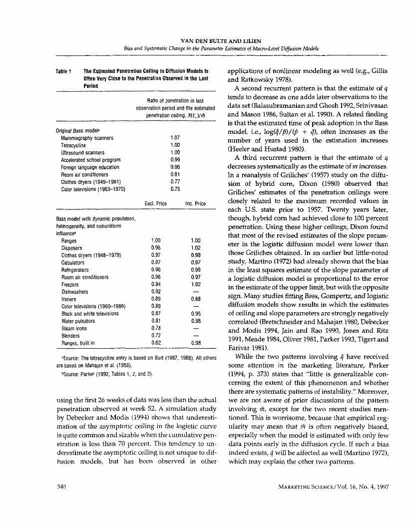
Three curious patterns exist across the applications of the Bass model and its variants. F i t , the estimated ceiling A often approximates the cumulative number of adopters observed in the last period used in the es- timation, Xft +), where t + denotes the last observation period. The pattem occurs with the original Bass model, as well as with more flexible versions allowing for dynamic population size, non-uniform influence, and price effects (Table 1). The finding that X(t+)/A = 1 in many applications raises the possibility of a sys- tematic downward bias in the estimate of the adoption ceiling or market size (A/m < I), since X(t+) 5 m by definition. The pattern in Table 1 is not conclusive, though, since it is conceivable that in all these studies the market was already close to saturation, in which case an unbiased estimator would produce the ob- served result, X(t+)/lfi -; 1. Two recent studies pro- vide more compelling evidence that underestimation does indeed often occur. Analyzing weekly adoption data for 19 different food items using six different models, including the Bass model, Hardie, Fader, and Wismewski (forthcoming) found that in more than 70 percent of the cases, the penetration ceiling estimated

VAN DEN BULTE AND LlLIEN Bias and Systematic Change in the Parameter Estimfc3 of Marno-Lewl Diffusion Models

Table 1 The Estimated Penetration CeillnQ in Diflusion Models Is Oflen Very Close to the Penetration ObSe~ed i n the Last Periotl

Ratio of penetration in last observation period and the estimated

penetration ceiling, X(tA)/r f i

Original Bass modela Mammography scanners Tetracycline Ultrasound scanners Accelerated school program Foreign language education Room air conditioners Clothes dryers (1949-1961) Color televisions (1963-1970)

Excl. Price Inc. Price

Bass model with dynamic population heterogeneity, and nonuniform influence0

Ranges Disposers Clothes dryers (1948-1979) Calculamrs Refrigerators Room air conditioners Freezers Dishwashers Ironers Color televisions (1960-1986) Black and white televisions Water pulsators Steam irons Blenders Ranges, built in

'Source: The tetracycline ently is based on Burt (1987. 1986). All others are based on Mahaian et at. (1986).

QSource: Parker (1992. Tabies 1. 2. and 3).

using the first 26 weeks of data was less than the actual penetration observed at week 52. A simulation study by Debecker and Modis (1994) shows that underesti- mation of the asymptotic ceiling in the logistic curve is quite common and sizable when the cumulative pen- etration is less than 70 percent. This tendency to un- derestimate the asymptotic ceiling is not unique to dif- fusion models, but has been observed in other

applications of nonlinear modeling as well (e.g., Gillis and Ratkowsky 1978).

A second recurrent pattern is that the estimate of q tends to decrease as one adds later observations to the data set (Balasubramanian and Ghosh 1992, Srinivasan and Mason 1986, Sultan et al. 1990). A related finding is that the estimated time of peak adoption in the Bass model, i.e., log(g/p)/(@ i r j ) , often increases as the number of years used in the estimation increases (Heeler and Hustad 1980).

A third recurrent pattern is that the estimate of q decreases systematically as the estimate of m increases. In a reanalysis of Griliches' (1957) study on the diffu- sion of hybrid corn, Diion (1980) observed that Griliches' estimates of the penetration ceilings were closely related to the maximum recorded values in each U.S. state prior to 1957. Twenty years later, though, hybrid corn had achieved close to 100 percent penetration. Using these higher ceilings, Dixon found that most of the revised estimates of the slope param- eter in the logistic diffusion model were lower than those Griliches obtained. In an earlier but little-noted study, Martino (1972) had already shown that the bias in the least squares estimate of the slope parameter of a logistic diffusion model is proportional to the error in the estimate of the upper limit, but with the opposite sign. Many studies fitting Bass, Gompertz, and logistic diffusion models show results in which the estimates of ceiling and slope parameters are strongly negatively correlated (Bretschneider and Mahajan 1980, Debecker and Modis 1994, Jain and Rao 1990, Jones and Ritz 1991, Meade 1984, Oliver 1981, Parker 1993, Tigert and Farivar 1981).

Whiie the two patterns involving r j have received some attention in the marketing literature, Parker (1994, p. 373) states that "little is generalizable con- cerning the extent of this phenomenon and whether there are systematic patterns of instability." Moreover, we are not aware of prior discussions of the pattern involving m, except for the two recent studies men- tioned. This is worrisome, because that empirical reg- ularity may mean that m is often negatively biased, especially when the model is estimated with only few data points early in the diffusion cycle. If such a bias indeed exists, 4 will be affected as well (Martino 1972), which may explain the other two patterns.

VAN DEN BULTE AND LILlEN Bias and Systonntk Change in the Parameter Estimates of Macro-leoel Dilfusion Models

This paper shows that in data structures similar to those of prior diffusion studies, the parameter esti- mates change systematically when one adds later data points to the data set, and that f i and p? are generally biased downwards, with cj biased upwards. We also show that these estimation problems need not result from model misspecification: Biases and systematic changes can occur even when the diffusion process truly follows the Bass model.

(Seber and Wid 1989). In addition, the characteristics of the NLS estimator, such as parameter bias and cor- relation matrix, are local, i.e., they depend on the true but unknown values of the parameters (Ivanov 1997). In sum, NLS estimates can be quite poor and biased when obtained from data sets with few and noisy ob- servations, but there is no theory to predict their be- havior in finite samples (Gillis and Ratkowsky 1978, p. 94). Hence, one cannot derive a practical, exact closed-form expression of the &rection and size of the

2. Nonlinear Least Squares bias and use this expression to adjust one's estimates (Box 1971). Nevertheless, a few informative theoretical Regression Theory and results exist. Let the nonlinear regression model for the

Hypotheses Bass specification (e.g., Equation (4)) be represented as:

2.1. NLS Regression Theory x(t) = g(t, e) + dt), where The two most common NLS-based estimation ap-

0 = the 3 x 1 parameter vector (m, q, p)', and vroaches for the Bass model are those of Srinivasan and Mason (1986) and Jain and Rao (1990). Both use dt) = error term, i.i.d. N(O,02). the same statistical estimation technique (NLS), but ap- ply it to slightly diferent model operationalizations.

Further, let

Defining x(t) as the number of adopters in period t, the V = the t+ x 3 matrix of first derivatives Jg(t)/aff, Srinivasan-Mason approach uses: (t = 1 ,..., t+ ;r = l,2,3),

x(t) = m[F(t) - F(t - 1)l + ~ ( t ) , (4) W, = the 3 x 3 matrix of second derivatives

and the Jain-Rao approach uses: #g(t)/aO,aff, (r, s = 1, 2,3), and

x(t) = [m - X(t - l ) l [F(t) - F(t - 1)1/ d = the t+ x 1 vector with elements

1(1 - Fft - 1)l + ~(t) , (5) k((V""9-1w~)r

where where all derivatives are evaluated at the hue param- eter values. Box (1971) derived an approximation of

~ ( t ) = an independently distributed error term, and the bias of the NLS estimator for 6, denoted as b ;- F(t) = the cumulative distribution function of E I ~ - 01, which can be expressed as:

adopters obtained from integrating Equation (2) assuming F(0) = 0;

= [1 - exp(-(p+q)t)l/ll + (qlp) exp(- (p + q)t)l. (6)

These functions are nonlinear in the parameters, so NLS rather than OLS must be used to obtain the least squares estimates. This has an important implication for the properties of these estimates, because the NLS estimator is not unbiased but only consistent. Param- eter estimates converge in probability to the true val- ues only as the number of observations approaches in- finity (for any given error variance) or as the error variance approaches zero (for any fixed sample size)

Cook, Tsai, and Wei (1986) later showed that extreme data points can have a substantial influence on the ex- pected bias b. Note that the values of (V'V)-' will be large when the columns of V are nearly linearly de- pendent, indicating that the data are not sufficiently rich to clearly identify each parameter in the model, a phenomenon called ill-conditioning (Belsley 1990). In linear regression, where V corresponds to the design matrix, ill-conditioning often takes the form of collin- earity and emerges when the regressors are too highly correlated to clearly identify all parameters or when, for a given pattern of correlation, the variability in the

VAN DEN BULTE AND LILIEN Bins and Systmt ic Change in the Parameter Estimates of Macro-Leuef Diffusion Models

regressors is too low (Belsley 1990, Mason and Perreault 1991). Note that ill-conditioning does not lead to bias in linear models because all matrices Wt, and hence d, are zero.

Research experience with nonlinear growth models documents the effect of these factors. Seber and Wid (1989) describe two problems. First, the growth path may not have a large enough signal-to-noise ratio to identify more than one hazard parameter (p. 336). Sec- ond, the data may not cover a sufficient range to iden- tify the ceiling parameter separately from the hazard parameter(s). Data from the early part of a diffusion process provide information confounding hazard and ceiling parameters, resulting in large covariances and poor point estimates (pp. 111-115). Berkey (1982, p. 959) experienced similar problems and, in line with the formal results obtained by Cook et al. (1986), re- marked that "if the last . . . observations are missing, the least squares method may not have enough infor- mation to estimate the asymptote." In another appli- cation, Gillis and Ratkowsky (1978) found that the es- timate of the asymptotic ceiling was often not only imprecise but also too low, i.e., the ceiling was under- estimated. These results suggest that problems are more likely to arise when one stops observing the dif- fusion process before it is completed such that X(t ,f < m, a situation commonly referred to as censoring or right-censoring.

In sum, the statistical literature indicates that the NLS Bass parameter estimates are likely to be biased even when the model is correctly specified, and that this bias is related to both the size of the error variance and the lack of richness of the data. Practical applica- tions of NLS regression to growth models suggest that problems are likely to occur in situations with: (i) too few observations, (ii) early censoring, and (iii) a little informative pattern in the data resulting in a poor "signal-to-noise" ratio. All three situations cause ill- conditioning, making parameter estimates sensitive to the addition or deletion of observations, and increas- ing the likelihood of sizable bias in the NLS estimates of Bass diffusion parameters.

2.2. Research Hypotheses Our review of the literature on diffusion modeling (§I) and NLS regression (52.1) suggests a number of hy- potheses about systematic changes and biases. While

we focus in this study on the Bass model and NLS estimation, we expect that similar problems exist with other diffusion models with an unknown ceiling and other estimation procedures using aggregate data.

Systematic Change. We propose three hypotheses on systematic change in the parameter estimates oc- curring as one adds later observations to the data set. We frame our hypotheses in terms of changes in both the number of observations and the amount of censor- ing, since the research reviewed above suggests that both affect the quality of estimates. Note that the num- ber of observations and the extent of censoring are closely related, because the amount of censoring is the gap between the true ceiling and the observed pene- tration, which can be represented as [m - X(t +)I/m. Since m is constant in the Bass model, changes in cen- soring are fully captured by changes in X(t +). Increases in t + result in non-negative changes in X(t +), meaning that the number of observations and the extent of cen- soring are closely linked. But it is possible to have a large value of t + and stiU have a high degree of cen- soring if the d i i s i o n process is slow, so we separate the effects in our hypotheses:

H Y P O T ~ S I S 1. fi increases as (a) the number of obser- vations increases and as (b) censoring decreases.

HYTOTHESIS 2. Lj decreases as (a) the number of obser- vations increases and as fb) censoring decreases.

HYPOTHESIS 3. f3 increases as (a) the number of obser- vations ittcreases and as (b) censoring decreases.

HI and H2 are in line with the findings of Debecker and Modis (1994), though their study did not distin- guish between the two effects (a) and (b). As indicated in the literature review in $1, evidence in favor of H2a can be found in a few marketing studies as well. Except for an application reported in Sultan et al. (1990), we are not aware of either analytical or empirical prior support for H3, but include it based on our own experience.

Size of Bias. We propose three hypotheses regard- ing the extent of bias and its causes. The hypotheses are derived from statistical theory and are known to be approximately true, conditional on the data struc- ture and the hue parameter values. Hence, what we

VAN DEN BULTE AND LILIEN Bins and Systmtic Change in the Parameter Esfimntes of M a c r ~ L e w l Diffusion Models

test is not whether these hypotheses are truein general, but whether they hold for the type of data structures encountered in diffusion research. Although the liter- ature reviewed in §1 suggests that m may often be un- derestimated and q overestimated, formal statistical theory does not exclude the reverse, and we leave the direction of the bias open as a question to be answered by the hypothesis tests.'

HYPOTHESIS 4. Higher error variance causes larger bi- ases in (a) f i , (b) 4, and (c) 8.

HYPOTHESIS 5. A smaller number of observations causes larger biases in (a) &, (b) 4, and (c) e.

HYPOTHESIS 6. Earlier censoring causes larger biases in (a) f i , (b) 4, and (c) p. The systematic change and bias hypotheses are inter- related once one knows the direction of the bias. For instance, if H6a is true and if m is typically underesti- mated, then Hlb should also hold. We test HI-H3 on both real and simulated data. We test H4-H6 on sim- ulated data only, since one must know the true data generating process to idenhfy and quantlfy bias.

3. Empirical Analysis We test the three change hypotheses using a number of well-known data sets. We first estimate a three- parameter Bass model for each data set using NLS, at different levels of t,. Next, we pool the estimates into a panel and test the hypotheses by modeling the change in the estimates as a function of the changing levels of t + and X( t+) . Such analysis addresses not

'In a preliminary analysis, we applied Box's bias approximation to the Srinivasan-Mason aperationalization of the Bass model for dif- ferent values of p, q, error variance, and number of observations. In most cases, the approximation predicted a downward bias in P. Of- ten, it predicted an upward bias in 4. We did not obtain a predicted downward bias for A, however. Because these analytical hut ap- proximate results run somewhat counter to prior reported research results, we do not specify the direction of the bias in H4-H6. For almost all the cases we examined, the predicted bias obtained using Equation (7) behaved according to hypotheses H4 and HJ us stated here. Regardless of the direction, the bias tended to be smaller as i, increased and as the error variance decreased. The majority of ex-

ceptions happened for situations in which t+ was prior to the dif- fusion m e ' s inflection point.

only whether there is support for the posited relation- ships, but also how strong the effects are. To make our conclusions as general as possible, we use data sets for a variety of innovations from different time periods obtained using different data collection methods by different researchers.

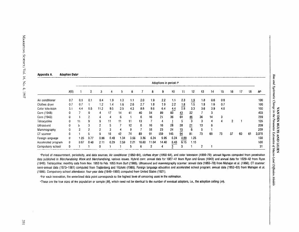
3.1. Diffusion Data and Modeling To minimize data problems and to have the results be representative of the published literature, we used four criteria when building our database. (1) Data must have been analyzed previously and published by other researchers. Thus, diffusion researchers should be fa- miliar with the data or with the studies in which they were used. (2) Data sets must contain at least 10 ob- servations, at least one of which comes after the inflec- tion point, to reduce the risk of nonconvergence and random parameter instability due to extreme data sparseness (Heeler and Hustad 1980, Srinivasan and Mason 1986). (3) The size of the population or sample, say M, must be known and constant, to reduce the risk that the number of evenhlal adopters m (m 5 M) changes over time. (4) Adoptions must be distin- guished from multiunit purchases or replacements by previous adopters, because the Bass model assumes a binary adoption process.

Appendix A lists the data we used. They cover a variety of situations: Adopters range from households, to professionals, to businesses and institutional orga- nizations, while the innovations range from an inex- pensive drug, to larger ticket items such as consumer durables, to radical and expensive innovations such as medical imaging equipment. The data originate from different streams within diffusion research: sociology, marketing, economics, education, and political science. We rejected data from 19 other studies because they did not meet one or more of our criteria.

For each data set, we estimated the three-parameter Bass model with NLS using both the Srinivasan-Mason and the Jain-Rao operationalization. Since NLS results are sensitive to the cho~ce of starting values, we used a grid search for p and q. We used M as the starting value for m , and only when we did not reach conver- gence within 100 iterations did we bring the starting value down toward X(t+) . We constrained the param- eter estimates to be non-negative. We repeated the pro- cedure varying t ,. We chose the minimum value oft ,

VAN DEN BULTE AND LILIEN BiDs and Svstmatic Chnnae in the Parameter Estimates o f Macro-he1 Difision Models

so that the shortest time series still contained at least p, = scale-free elasticity with respect to kth one period beyond the inflection point and was at least regressor, used to test our hypotheses, 10 G o d s long. We then added one period at the time to the estimation sample, and repeated the estimation procedure above. We estimated 56 different sets of pa- rameters for each operationalization.

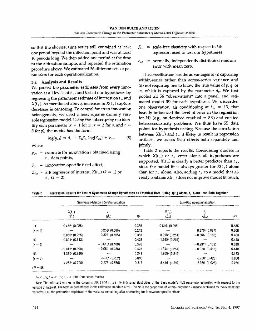
3.2 Analysis and Results We pooled the parameter estimates from every inno- vation at all levels of t +, and tested our hypotheses by regressing the parameter estimate of interest on t + and X( t+ ) . As mentioned above, increases in X ( t + ) capture decreases in censoring. To control for cross-innovation heterogeneity, we used a least squares dummy vari- able regression model. Using the subscript by r to iden- t i f y each parameter ( r = 1 for m, r = 2 for q, and r = 3 for p), the model has the form:

log[yw1 = 6, + &8kr log[Zikt1 + eirt, ( 8 )

where

e , , = normally, independently distributed random error with mean zero.

This specification has the advantages of (i) capturing within-series rather than across-series variance and (ii) not requiring one to know the true value of p, q, or m, which is captured by the parameter 6.. We first pooled all 56 "observations" into a panel, and esti- mated model ( 8 ) for each hypothesis. We discarded one observation, air conditioning at t + = 13, that heavily influenced the level of error in the regression for HI (e.g., studentized residual = 8.9) and created heteroscedasticity problems. We thus have 55 data points for hypothesis testing. Because the correlation between X( t +) and t + is likely to result in regression artifacts, we assess their effects both separately and jointly.

yi, = estimate for innovation i obtained using able 2 reports the results. Considering models in

t . data voints. which X(t +) or t + enter alone, all hypotheses are 7

6, = innovation-specific fixed effect, supported. X ( t + ) is clearly a better predictor than t + , since the model fit is always greater for X ( t + ) alone . -

Zi, = kth regressor of interest, X ( t + ) (k = 1 ) or than for t + alone. Also, adding t + to a model that al- t + (k = 2) , ready contains X(t +) does not improve model fit much,

Table 2 Repression Results for Test of Systematic Change Hypotheses an Empirical Data. Using 4t+) Alone, t, Alone, and Bolh Together

Srinivasan-Mason operationalization Jain-Rao operationaiization

Hi O.44Zc (0.085) - 0.335 0.610r (0.095) - 0.435 ( r = 1) - 0.25W (0.068) 0.212 - 0.376* (0.077) 0.306

0.856' (0.225) -0.327 (0.165) 0.381 0.99Sc (0.254) -0.306 (0.186) 0.463 H2 -0.891. (0.142) - 0.423 - 1.36W (0.205) - 0.448 (r = 2) - -0.618. (0.108) 0.376 - -0.9311 (0.159) 0.389

-0.8131 (0.390) -0.062 (0.286) 0.423 - 1.344< (0.254) -0.010 (0.415) 0.448 H3 1 .3801 (0.326) - 0.248 1.70@ (0.545) - 0.153

(r = 3) - 0.635b (0.262) 0.098 - 0.766' (0.423) 0.058 4.258' (0.790) -2.275 (0.580) 0.417 5.410. (1.397) - 2.930 (1.026) 0.266

(N = 55)

aa < .05; .r 01: a c ,001 (one-sided ttests).

Nole. The left-hand entries in the columns Xt,) and 1, are the estimated elasticities of the Bass model's NLS parameter estimates with respect to the variable of interest. The term in parentheses is the estimated standard error, The R2 is the proportion of within-innovation variance explained by the expianator] variables, i.e.. the proportion explained of the variance remaining aiter controlling for innovation-specific effects.

VAN DEN BULTE AND LILIEN Bias and Systematic Change in the Parameter Estimates of Macro-Lml Diffusion Models

but leads to a sign reversal for the effect of t+ . This is probably due, at least partly, to cohearity (cf. Darliigton 1968). For X(t + ), all the coefficients have the expected sign and the null is rejected for all three hypotheses at the a = .05 level or better, whether only controls for the number of observations or not. The effects in models featuring Xft +) only are suable: A 10 percent increase in observed penetration is associated with, roughly, a 5 percent increase in estimated market size A, a 10 percent decrease in r j , and a 15 percent increase in p. We also ran analyses controlling for dif- ferences in data periodicity (monthly, semi-annual, an- nual, and four-year) and for the varying number of observations per innovation, with essentially the same conclusions.

4. Simulation Analysis To test the three bias hypotheses and to check whether systematic changes can occur even in absence of any misspeafication, we conducted a Monte Carlo simu- lation study. We manipulated the three sources of ill- conditioning identified above and error variance, and combined them into a full-factorial design. We manip- ulated the signal-to-noise ratio by varying the shape of the true diffusion curve through the q / p ratio (signal) over four levels and by varying the level of error var- iance (noise) over five levels.' We varied the length of the data series used in the model estimation, t , , over four levels: 10, 12, 14, and 16. To avoid the problems in the empirical analysis and to manipulate censoring independently from t,, we made the speed of diffu- sion low versus high by reducing the values of both p and 9 by 20 percent, leaving their ratio unchanged. Thus, our design has 160 cells: Signal (4) x Noise (5)

'Assuming that the true errors are proportional to the probability of adoption in period t (Debecker and Modis 1994, Dixon 1980, Srinivasan and Mason 1986), we created the perturbed adoptiondata x(t) using a multiplicative error speciiication: x ( f ) = yl(t)ctf), where yl(f) are the true adoption data series generated from the Bass model and dt) are random errors generated from a log-normal distribution with mean 1 and variance expia21 - 1. We selected five levels of error variance: o equaling .06, .24, .42, .60, and .78. The three highest values reflect the levels of error variance found in the 12 data sets. We included the two lower values to check whether we attained consistency as $ -f 0 regardless of the number oi observations in- cluded, as NLS theory posits.

x Speed (2) x Number of observations (4). For each cell, we created 50 data series for which we estimated the Bass model using NLS, resulting in 8,000 estima- tions; 7,085 of these converged. We used the Srinivasan-Mason operationalization for both data creation and parameter estimation. (Details of the de- sign and procedures are available on request.)

Bias Analysis. Table 3 reports how the cell medi- ans for the estimates relate to the factors driving ill- conditioning. Overall, the results confirm the impor- tance of ill-conditioning on the performance of the NLS estimator: A small number of periods, a high degree of error, and low diffusion speed result in a downward bias for A and p and an upward bias in r j . The size of the biases can be quite substantial. For conditions

Table 3 Factors Driving Ill-Conditioning Affect the Parameter Estimates in the Simulation: Analysis of Variance on the Percentage Deviation of Cell Medians from True Value'

Base q4p ratio

2 5

50 Low speed Error variance

Moderate ( 0 = .42) Average ( 0 = .60) High (0 = .78)

Number of observations t, = 14 t* = 12 t* = 10

R2 ( N = 128)

' 0 < .05; a < .01; ( u c ,001 (two-sided ttests).

W e regressed the cells' median percentage deviation on the factors ma- nipulated in the simulation using a main effects dummy regression. As ex- pected from NLS theory, the NLS regressions always attained consistency as the error approached zero, regardless of the number of observations included, speed of diffusion, or q/p ratio. Because such a pattern is not compatible with a main effects specification, we excluded the lowest level of error variance (o = 0.06), reducing the number of cells from 160 to 128. The base condition is a "best case" with parameter values p = 0.03 and q = 0.38 (q/p = 13, high speed), low error variance (0 = 0.24). and t.. = 16.

VAN DEN BULTE AND LILlEN Bias and Systematic Change in the Parameter Estimates of Macro-Leuel Diffusion Models

representative of many marketing applications (p = 0.024; q = 0.304; a = 0.60; and t + = lo), m can be underestimated by 20 percent, p underestimated by the same amount, and q overestimated by 30 percent. These biases are larger than those reported by Srinivasan and Mason (1986, p. 173, who performed a small simulation analysis (N = 50) and concluded that "the biases in the parameter estimates p, 4, and

(e.g., I 6 - p l /p) were less than 7%: Their results,

however, were based on a single set of parameter set- tings, less serious censoring and less noise in the data than the average in our 12 data sets and simulation. When using similar parameter values, censoring, and noise levels, we found results' similar to those of Srinivasan and Mason. We conducted formal tests of H4, H5, and H6 using the same model as in Table 3, but with 2 and t+ entering as continuous regressors. These tests reject all but one of the null hypotheses at a < ,001 (two-sided t tests) and show that the direction of the biases is the same as in Table 3. The exception is H6c: Earlier censoring, operationalized as low speed, is not significantly associated with the bias in p.

Systematic Change Analysis. We also used our simulation results to perform a second test of HI, HZ, and H3 under conditions where misspecification can be excluded as a confounding factor. We used the same procedure as in the analysis of the empirical data: a least squares dummy variable model with log- transformed variables (Equation (8)). As the dummy variables J,, capture the effects of the q/p ratio, low ver- sus high speed, and the true error variance, these three variables cannot enter in the models. We reshicted the data to parameter estimates generated from data series with a equaling .42, .60, or .78, noise levels one is more likely to encounter in practice, and discarded 40 data points that were the only remaining member of their series, reducing the sample to 3,946 data points. Hlb, H2b, and H3b are again strongly supported. The elas- ticities of the parameter estimates with regard to X ( t + ) as the sole predictor are very similar to those found in the empirical analysis for the Srinivasan-Mason oper- ationalization: about 0.5 for m, -0.7 for 4, and 1.3 for p, all with a < 0.001 (one-sided t tests).

5. Can Model Misspecification Explain the Occurrence of Systematic Changes?

The simulation study shows that the systematic change in the parameter estimates observed in the empirical- study can occur even when the model is correctly spec- ified. The analysis of bias indicates why: p and m tend to be underestimated, and q underestimated, but these biases become smaller as one adds observations to the data set Hence, the systematic changes can be ex- plained as the result of better conditioning and de- creased bias. There are some indications that condi- tioning improvement and bias reduction may indeed have driven the changes we observed. The fact that m, $, and p change more for the more complex Jain-Rao operationalization suggests that the changes may have originated from a gap between the richness of the data and the complexity of the regression models. Formal conditioning analysis (Belsley 1990) reveals that the Bass model parameters we estimated show indications of ill-conditioning. For seven of the data sets, the rate parameters p and 9 load quite heavily (95 percent or higher) on the same component of the parameter cor- relation matrix. On the other hand, the typical condi- tion number was well below 30, the value suggested by Belsley (1990) to distinguish large from small condition numbers in OLS (we are not aware of any similar rule of thumb for NLS). Thus, though the sys- tematic change in parameter estimates of the 12 inno- vations may have originated from ill-conditioning, the evidence is not conclusive. An alternative explanation for the observed systematic changes is the presence of various types of model rnisspecification, such as popu- lation growth, omitted variables, and unobsemed het- erogeneity. In this section, we assess the merits of this alternative explanation.

One explanation for the changes in m that occur as one adds later data points is that the populations, and hence the true penetration ceilings WI, increase over time. This is a viable explanation for systematic changes in many studies using U.S. sales data for con- sumer durables over the period 1950-1985, when the U.S. population increased from about 150 million to about 240 million. However, population growth cannot explain systematically changing parameter estimates in

VAN DEN BULTE AND LILIEN Bias and S y s t m t i c Change in the Parameter Estimates of Macro-Lewl Diffusion Models

studies using penetration data or adoption data from samples or censuses with a fixed size, as is the case with al l 12 data sets we used.

Omitting time-varying variables is a second cause of misspecification that may explain systematic changes in parameter estimates. The Bass model does not ac- count for the effect of declining real prices, increasing distribution penetration, and improving product per- formance. Such variables may lead the penetration ceiling to increase even in a population of fiwed size (e.g., Kalish and Lilien 1986). For instance, as the real price of refrigerators drops over time, lower-income households become able to afford them, leading m to increase. Under such conditions, one can expect that the NLS estimate A will not only systematically in- crease, but also be biased downwards (Xie et al. 1997). Omitted variables may also affect the rate parameters. One can expect omitted variables that are positively (or negatively) related to the hazard rate and increase (or decrease) at a decreasing (or increasing) rate to result in a downward pressure on the estimate of q as one adds more observations to the data set.3 For instance, the fact that product performance often in- creases more rapidly in the first years after launch than in later periods (Bayus 1994, Trajtenberg 1990) and is likely to affect the decision to adopt may explain why p and q^ in a traditional Bass mode1 often change as one extends the number of years used in the estimation.

A third cause of model misspecification that might explain systematic changes in the parameter estimates is unobserved heterogeneity. For instance, assume all people have the same intrinsic tendency to adopt, cap- tured by p, but differ in their susceptibility to social contagion, captured by q. At any time, those with the highest q have a higher adoption hazard h(t) and tend to adopt earlier. As a result, the population of remain- ing eventual adopters is increasingly made up of peo- ple with a lower q as time progresses. As a result, q^ may decrease as one extends the number of periods in the estimation. Unobserved heterogeneity in p can

3This is in line with the generalized Bass model or GBM specification (Bass et al. 1994). If one estimates a Bass model on diffusion data generated by a GBM process, then the estimates of p and q will be biased but they mil l not change systematicaUy if the omitted vari- ables change at a constant rate.

induce a similar downward pressure on the slope of the estimated hazard rate (cf. Blossfeld et al. 1989), and hence affect the estimate of q .

If the tendency for parameter estimates to change as one adds later observations to the data set were due mostly to model misspecification rather than the result of ill-conditioning, then the changes observed in 53.2 should be less severe once one makes the model more flexible. To assess whether this indeed is the case, we analyzed the behavior of three extensions of the Bass model: the non-uniform influence model, which allows the social contagion effect to decrease as the level of penetration goes up (Easingwood et at. 1983), the non- uniform influence model with a multiplicative control for the hazard rate (e.g., Parker 1992), and the gener- alized Bass model (Basset al. 1994). We collected data on control variables (nominal and deflated price, av- erage income, and hedonic price or profitability) for six of the 12 innovations in Appendix A (color TVs, dryers, air conditioners, CT scanners, and the two hybrid corn series), and used the same proce- dure as before to test HI-H3. The results (details avail- able on request) show that the extended models exhibit the same pattern as the Bass model: Ift increases and 4 decreases as the observed cumulative penetration increases. (As we had to fix the value of p in a few cases to obtain estimation convergence, we did not assess changes in p.) Moreover, we found the extended models to be more sensitive to changes in the under- lying data than the Bass model. These results in- dicate that nonuniform influence or omitted variables are unlikely to account for the systematic changes re- ported in 53.2. Rather, the results provide further sup- port to the ill-conditioning explanation: Making the model specification more complex and increasing the number of parameters make the regression problem even more ill-conditioned and the estimates more unstable.

In conclusion, both estimation problems and model misspecification can explain the systematic changes observed in the empirical analysis. Because better spec- ified models are often also more complex, their esti- mation is more problematic. As a result, developing more complete models to reduce misspecification bias may actually lead to even more pronounced systematic changes.

VAN DEN BULTE AND LILlEN Bias and Systematic Change in the Paramefer Estimates of M a n o - h e l Diffusion Models

6. Discussion Using both empirical and synthetic data, we have shown that systematic changes occur in the nonlinear least squares (NLS) parameter estimates of the Bass model. We have shown using synthetic data that these estimates are biased and that these biases are related to ill-conditioning: A small number of observations, a high degree of error, and early censoring result in a downward bias for #I and f j and an upward bias in $. Although in empirical studies the systematic change and bias problems may be aggravated by model mis- specification, the latter is not required: Ill-conditioning alone can generate systematic change and bias. We also found that, given the ill-conditioning of the data, it is hard to address the model misspecification problem by making the model more flexible and adding free pa- rameters. Making the model more complex can actu- ally aggravate the tendency for parameter estimates to change systematically as one extends the data set. Based on NLS theory, we suspect that increasing model complexity can also increase the bias stemming from in-conditioning, but we did not directly assess this conjecture. While we focused on the NLS estima- tion procedure and the Bass model here, similar prob- lems are likely to exist with other macro-leveldiffusion models featuring an unknown ceiling and other esti- mation procedures (e.g., MLE, 0LS)-a poor signal-to- noise ratio degrades the performance of any estimator. Below, we discuss the relevance of the bias and sys- tematic change problems and make a few suggestions.

6.1. Relevance for Predictive, Prescriptive, and Descriptive Uses

Some researcherss may be willing to trade off some bias to gain the benefits from a useful model. Others may correctly point out that ill-conditioning is not a major issue if one is only interested in the shapeof thediffusion m e or its inflection point, since ill-conditioned param- eter estimates can vary substantially as a consequence of relatively minor perturbations in the data while the predicted curves are very similar in shape over the range covered by the estimation data. These points should be viewed with caution because the bias and systematic change problems are serious enough to make predictive, prescriptive, and descriptive applications of Bass-type models suspect.

Market Size Assessment (Predictive Use Outside the Data Range). Our results indicate that managers interpreting A as the eventual penetration a new prod- uct or technology can be expected to achieve may se- riously underestimate their market potential. Manag- ers who believe the output of the model might invest insufficient resources in product and market develop- ment, so that the belief that the market is close to sat- uration becomes a self-fulfilling prophecy.

Marketing Strategies (Prescriptive Use). Decision makers may also be misguided by the inflated 4, lead- ing them to underspend on advertising and overuse penetration pricing. Normative models of advertising in a diffusion environment generally suggest high ini- tial levels of advertising followed by a gradual decline (e.g., Horsky and Simon 1983). How fast advertising should decrease depends on the strength of the word- of-mouth effect: The higher q, the faster social conta- gion takes over the demand-inducing role of advertis- ing, and the faster one can reduce one's spending. Our results indicate that, since the true q is not as high as its estimate, taking r j at face value could result in un- derinvestments in advertising. The inflated word-of- mouth effect may also result in overusing penetration pricing. Horsky (1990) derived the following decision rule for monopolists: Penetration pricing is optimal if word-of-mouth effects are so large that q > (2p + kf/4F(t), where k stands for the cost of capital. If q is smaller, price s k i i n g is more profitable. From Horsky's formula, it is clear that an inflated r j can lead firms to choose penetration pricing too often. Estimat- ing a three-parameter Bass model for clothes dryers over the period 1950-1964, for example, one would es- timate the critical cost of capital for clothes dryers to be 49 percent. Estimating p and q from a two- parameter model in which m is exogenously fixed to the actual penetration in 1979 (61.5 percent), the critical cost of capital would be only 9 percent, a value at which most monopolists would skim rather than penetrate.

Diffusion Acceleration (Descriptive Use). Many managers and academics believe that diffusion cycles are shortening. Olshavsky (1980) and Takada and Jain (1991) reported that the slope parameter of the hazard rate in a diffusion model is positively related to the

VAN DEN BULTE AND LILIEN Bins and Systonatic Chonge in the Parameter Estimates of Mono-Level Dijjisian Models

year of launch for consumer durables. Others, how- ever, have not found evidence that more recent con- sumer durables have a higher diffusion rate (e.g., Bayus 1992). Our results suggest that evidence sup- porting diffusion acceleration may be at least partly due to a method artifact, since both Olshavsky (1980) and Takada and Jain (1991) used more data points to estimate diffusion parameters for earlier innovations than for more recent ones. Hence, the bias we have identified may have been higher for recent than for old innovations, artificially inflating the former's parame- ter estimates 4, which Olshavsky (1980) and Takada and Jain (19911 used as a measure of diffusion speed. To investigate this competing explanation, we re- gressed the parameters reported in these two studies against not onty the year each innovation was launched, but also against the number of observations used to estimate these parameters. We found that the positive relationship between diffusion speed and year of launch disappears once one controls for the number of observations used in the estimation (Table 4). This result cash some doubt on the accepted belief of ac- celerating diffusion cycles.

6.2. Methodological Suggestions The biases and systematic changes are not minor tech- nicalities that can be pratically ignored. Though ill- conditioning is a problem for which no quick fiw is available (Belsley 1990), one can make a few method- ological suggestions based on the extant literature and our &dings.

Simplifying the Model. Our results caution against estimating market potential using aggregate- level diffusion models. Across a variety of innovations, we found those estimates to be strongly driven by the level of adoption observed in the last period for which data are used. Using exogenous estimates of m ob- tained from market surveys, secondary sources, man- agement judgments, or other models can lead to better results (Mahajan et al. 1993, p. 391, Parker 1994). If multiple exogenous estimates of m are available, Trajtenberg and Yitzhaki (1989) suggest investigating how sensitive the other parameters and the shape of the diffusion curve are to these different values of m. Using an exogenous ceiling also linearizes the regression problem in the adoption domain (based on

Table 4 Prior Evidence That Dillusion Speed (qt Is Positively Related to Year of Launch Disappears When Controlling lor the Number of Observatians Used to Estimate the Dillusion Models

Model ? Model 2 Model 3 Year of launch Number of Observations Both Factorsb

Olshavsky (1980p ( N = 25) Intercept Year of launch Number of observations R2

Takada and Jain (?991)* ( N = 26) Intercept Year of launch Number of obse~ations R'

< 0.001.

*Note that the launch year effect becomes insignificant once one controls for the number of data points used to obtain the parameter estimates.

"he regression estimated is 0 = 6, + p, year + p, f a , and its nested variants. Oishavsky obtained the parameter estimate $from a logistic diffusion model (i.e.. p = 0) in which he fixed the ceiling rn exogenousiy as the maximum penetration achieved (i.e., m = X(t , ) ) . He reported slightly differentestimales for Modei 1, but the difference is very srnaii and the slatistical inference is not different from ours.

"We estimated the same regression models as for Olshavsky. Because Takada and Jain's data come from four countries, we aiso estimated alternative mooels in which we controiied for product and country effects. The results were similar and are not reported here. Takada and Jain estimated the slope parameter Q using the traditional three-parameter Bass model.

% , < "r - Appendix A. Adoption Data- 0)

Z Adoptions in period tb ?

.J

Air conditioner 0.7 0.1 0.1 0.4 1.9 1.3 1.1 2.0 1.9 2.2 1.1 2.3 9 1.8 0.6 0.8 100 Clothes dryer 0.7 0.7 1 1.2 1.4 1.6 2.6 2.7 1.8 1.9 2.2 1.5 1.8 1.6 0.7 100 Color ieievision 5.1 4.4 5.5 11.2 9.5 2.5 4.3 8.6 9.6 6.4 44 2.9 3.3 3.6 3.9 4.6 100 Corn (1948) 0 7 9 4 17 14 41 40 54 89 83 43 22 7 3 433 Corn (1943) 0 1 2 4 4 6 1 6 16 21 36 61 46 36 14 3 259 Tetracycline 0 11 9 9 11 11 11 13 7 4 1 5 3 3 4 4 2 1 125 Ullrasoiind 0 5 3 2 5 7 12 6 16 16 28 28 21 13 6 209 Mammography 0 2 2 2 3 4 9 7 1 6 2 3 2 4 1 5 6 5 1 209 CT scanner 0 1 5 9 18 42 74 89 91 159 146 94 81 73 69 73 57 60 61 3,078 Foreigrl language 0 1.25 0.77 0.86 0.48 1.34 3.56 3.36 6.24 5.95 6.24-% 1.25 100 Accelerated program 0 0.67 0.48 2.11 0.29 2.59 2.21 16.80 11.04 14.40 643 6.15 1.15 100 Cornpulsory school 0 1 1 0 1 1 5 6 2 4 3 3 1 2 1 31

"Period of measurement, periodicity, and data sources: Air conditioner (195[)-64), clothes dryer (1950-64), and color television (195679): annual figures computed from penetration data published in Merchandising Week and Merchandising. various issues. Hybrid corn: annual data for 1927-41 from Ryan and Gross (1943) and annual data for 1929-42 from Ryan (1948). Tetracycline: monthly data from Nov. 1953 l o Feb. 1955 from Burt (1986). Ultrasound and mammography scanner: annual data (1965-78) from Mahaian et al. (1986). CTscanner: semi-annual data (1973-1981) computed from Traitenberg and Yitzhaki (1989). Foreign language education and accelerated school program: annual data (1952-63) from Mahajan et ai. (1986). Compuisory schooi attendance: four-year data (1849-1902) computed from United States (1921).

Tor each innovation, the underlined data point corresponds to the highest level of censoring used in the estimation.

CThese are the true sizes of the population or sample (M), which need not be identical to the number of eventual adopters, i.e., the adoption ceiling (m).

VAN DEN BULTE AND LILIEN Bias and Systematic Change in the Parameter Estimates of Macro-Leuel Difusion Models

References Balasubramanian, Siva K. and Amit K. Ghosh (1992). "Classifying

Early Product Life Cycle Forms via a Diffusion Model: Prob- 1- and Rmpect3Intemational Journal of Research in Market- ing, 9, December, 345-352.

Bass, FrankM. (1%9), "A New Product Growth Model for Consumer Durables," Management Science, 15, January, 215-227. - , Trichy V. Krishnan, and Dipak C. Jain (1994). 'Why the Bass

Model Fits Without Decision Variables," Marketing Science, 13, Summer, 203-223.

Bayus, Bany L. (1992), "Have Diffusion Rates Been Accelerating Over Time?" Marketing Letters, 3, July, 215-226,

- (1994). "Optimal Ridng and Product Development Polides for New Consumer Durables," Zntmuztional lourn2 of Research in Marketing, 11, June, 249-259.

Bdsley, David A. (1990), Conditioning Dingnostics: Collineanty and Weak Data in Regression. New York: John Wiley.

Berkey, Catherine S. (1982). "Bayesian Approach for a Nonlinear Growth Model," Hiometrin, 38, December, 955961.

Blossfeld. Hans-Peter, Alfred Hamerle, and Karl Ulrich Mayer (1989), Ewnt Histoy Analysis: Statistical Theory and Applicnfions in the Socinl Sciences. Hillsdale, NJ: Lawrence Erlbaum Associates.

Box, M. 1. (1971). "Bias in Noniinear Estimation (with Discussion)," lournnl ofthe Royal Statistical Society, Ser. H, 33,2, 171-201.

Bretschneider, Stuart I. and Vijay Mahajan (198(3), "Adaptive Tech- nological Substitution Models," TechnologialF~recnstingand So- cinl Change. 18, October, 129-139.

Burt, Ronald S. (19861, Social Contogion and innovation. unpublished manuscript, Columbia University, New York.

- (1987) "Social Contagion and Innovation: Soda1 Cohesion Ver- sus Stmctural Equivalence," American Journal of Sociology, 92, May, 1287-1335.

Coleman, James S. (1964), Introduction to Mathemntical Sociology. Lon- don: Free Press of Glencw.

Cook, R. D., C.-L. Tsai and B. C. Wei (1986), "Bias in Nonlinear Re- gression," Biometrika, 73, December, 615423.

Darlington, Richard H. (1968). "Multiple Regressionin Psychological Research and Practice," Psychological Bulletin. 69.3. 161-182.

Debecker, A. and T. Modis (1994), "Determination of the Uncertain- ties in S-Curve Logistic Pits," Technological forecasting nnd Social Change, 46,153-73.

Dixon, Robert (1980), "Hybrid Cam Revisited," Econornetrica, 46, September, 1451-1461.

Easingwood, Christopher J., Vijay Mahajan, and Eitan Muller (1983). "A Non-Uniform Influence Innovation Diffusion Model of New Produd Acceptance," Marketing Science, 2. Summer, 275296.

Gillis, P. R. and D. A. Ratkorvsky (1978), 'The Behaviour of Esti- mators of the Parameters of Various Yield-Density Relation- ships," Biornetrics, 34, June, 191-198.

Griliches, Zvi (1957). "Hybrid Corn: An Exploration in the Econom- ics of Technological Change," Emnometrica, 25, Cktober, 501- 522.

Hardie, Bmce G. S., Peter S. Fader, and Michael Wkniewski (forth- coming), "An Empirical Comparison of New Product Trial Forecasting Models," lournaf of Forecasting.

Heeler, Roger M. and Thomas P. Hustad (1980), "Problems in Pre- dicting New Product Growth for Consumer Durables," Man- agement Science, 26, October, 1007-1020.

Horsky, Dan (1990). "A Diffusion Model Incorporating Product Benefits, Rice, Income and Information," Marketing Science, 9, Fall, 342-365.

- and Leonard S. Simon (1983). "Advertising and the Diffusion

of New Produds," Marketing Science, 2, Winter, 1-17. Ivanov, Alexander V. (19971. Asymptotic TheDy of Nonlimr Regres-

sion. Dordrecht: Kluwer. Jain, DipakC. and Ram C. Rao (1990). "Effect of Priceon the Demand

for Durables: Modeling, Estimation, and Findings," Journal of Business and Economic Statistics, 8, April, 163-170.

Jones, J. Morgan and Christopher I. Ritz (1991). "Incorporating Dis- tribution into New Product Diffusion Models," International lournal of Research in Mnrketing, 8, June, 91-1 12.

Kaiish, Shlomo and Gary L. W e n (19%). "A Market Entry Timing Model for New Technologies," ManRgment Science, 32, Fehm- ary, 194-205.

Mahajan, Vijay, Charlotte H. Mason, and V. Srinivasan (1986), "An Evaluation of Estimation Procedures for New Product Diffu- sion Models," in innooation Diffusion Models of New Product Ac- ceptance, Vijay Mahajan and Yoram W i d (Eds.), Cambridge, MA: Baliinger, 205232.

- , Eitan Muller, and Frank M. Bass 119931, "New-Praduct Dif-

fusion Models," in Handbook of Marketing, J. Eliashherg and G. L. Lilien (Eds.), Amsterdam: North-HoUand, 3494%.

Mansfield, Edwin (1961), "Technical Change and the Rate of Imita- tion," Econornetrica, 29, Odober, 741-766.

Mason, Charlotte H. and William D. Perreauk, Jr. (1991), "Coiline arily. Power, and Interpretation of Multiple Regression Anal- ysis," Journal of Marketing Research, 28, August, 268-280.

Martino. Joseph P. (197'21, 'The Effect of Errors in Estimating the Upper Limit of a Gmwth Curve," Technologtcal Forecasting and Social Change, 4.1. T-84.

iMeade, Niget (19%). 'The Use of Growth C m e s in Forecasting Market Development-A Review and Appraisal," International [ournnl ofForerasting, 3, October-December, 429-451.

Oliver, F. R (1981), 'Tracton in Spain: A Further Logistic Analysis," Journal of the Operational Research Society, 32, June, 499-502,

Olshavsky, Richard W. (1980), 'Time and the Rate of Adoption of Innovations," Journal of Consumer Resfarch, 6, March, 4254128.

Parker, Philip M. (1992). "Price Elasticity Dynamics Over the Adop- tion Life Cycle," loumal of Marketing Research, 29, August, 358- 367.

- (1993). "Choosing Among Diffusion Models: Some Empirical

Evidence," MDrketing Letters, 4, 1, 8144. - (1994). "Aggregate Diffusion Forecasting Models in Marketing:

A Critical Review," biternational Journal giFoiecasting, 10, 353- 380.

VAN DEN BULTE AND LIUEN Bios and Sysfematic Chunxe in the Parameter Estimntes of Mnno-Leuel Diffusion Models

Putsis, CViUiam P., Jr (1996), 'Temporal Aggregation in Diffusion of Diffwion of Consumer Durable G o d s in Pacific Rim Coun- Models of First-Time Purchase: Daes Choice of Frequency Mat- hies," Journal of Marketing, 55, Apd, 48-54. ter?" Technological Forecasting and Social Change, 51, March, 265- Tigert, Dougias and Behrwz Farivar (1981), 'The Bass New Product 279. Growth Model: A Sensitivity Analysis for a High Technology

Ryan, Bryce (1948). "A Study in Technological Diffusion," Rural So- Produd," fouml of Mnrkefing, 45, Fall, 81-90. ciology, 13, September, 273-284. Traitenberg, Manuel (1990). Economic Analysis of Product Innovation:

- and Neal C. Gross (1943). 'The Diffusion of Hybrid Seed Corn I?re Case of CT Scanners. Cambridge, MA: Itaward University in Two Iowa Communities," Rural Sociology, 8. March, 15-24. Press.

Seber, G. A. F. and C. J. Wild (1989). Nonlinear Regression. New York: - and Shlomo Y i a a k i (1989). 'The Diffusion of hovat ions: A John WiIey. Methodological Reappraisal," ,Journal of Business and Economic

Srinivasan, V. and Charlotte H. Mason (1986). "Nonlinear Least Statistics, 7, January, 35-47. Squares Estimation of New Product Diffusion Models," Mar- United States. Department of the Interior. Bureau of Education keting Science, 5, Spring, 169-178. (1921). Bienninf Surwyof Education, 1916-1918. Washington,DC:

Sultan, Fareena, John U. Farley, and Donald R. Lehrnann (1990). "A Government Printing Office. Meta-Analysis of Diffusion Models," Jouml of Marketing Re- Xie, Jinhong, X. Michael Song, Manin Sirbu, and Qiong Wang search, 27, February, 70-77. (1997). "Kalman Fitter Estimation of New Product Diffusion

Takada, Hirokazu and Dipak Jain (1991), "GossKational Analysis Models," Journal of Marketing Research, 34, August, 378-393.

Tkis paper was received April 22, 1996, and has been with the authors 13 months for 2 revisions; processed by Dick R. Wittink.