Bicontinuous Surfaces in Self-assembling Amphiphilic Systemsbiophys/PDF/LNP2002.pdf · Bicontinuous Surfaces in Self-assembling Amphiphilic Systems Ulrich Schwarz 1 and Gerhard Gompper

Bicontinuous Surfacesin Self-assembling Amphiphilic Systems

Ulrich Schwarz1 and Gerhard Gompper2

1 Max-Planck-Institut fur Kolloid- und Grenzflachenforschung, D-14424 Potsdam2 Institut fur Festkorperforschung, Forschungszentrum Julich, D-52425 Julich

Abstract. Amphiphiles are molecules which have both hydrophilic and hydrophobic parts. Inwater- and/or oil-like solvent, they self-assemble into extended sheet-like structures due to thehydrophobic effect. The free energy of an amphiphilic system can be written as a functional ofits interfacial geometry, and phase diagrams can be calculated by comparing the free energiesfollowing from different geometries. Here we focus on bicontinuous structures, where one highlyconvoluted interface spans the whole sample and thereby divides it into two separate labyrinths.The main models for surfaces of this class are triply periodic minimal surfaces, their constantmean curvature and parallel surface companions, and random surfaces. We discuss the geome-trical properties of each of these types of surfaces and how they translate into the experimentallyobserved phase behavior of amphiphilic systems.

1 Surfaces in Self-assembling Amphiphilic Systems

The subject of this article is the theoretical description of amphiphilic systems, which areone example ofsoft condensed matter. Soft matter is material that has a typical energyscale ofkBT ≈ 4 × 10−21J , wherekB is the Boltzmann constant andT ≈ 300K isroom temperature. For such material, perturbations arising from the thermally activatedmovement of its molecular components are sufficient to induce configurational changes,and entropy is at least equally important as energy in determining its material properties.The understanding of the underlyingmechanisms is essential for the application ofmanytechnologies in everyday life, including colloidal dispersions (paints, inks, food, creams,lotions), foams (beverages), liquid crystals (displays), polyelectrolyte gels (diapers) andsoaps (washing and cleaning). Moreover, the termsoft matteralso includes most bio-materials, for example blood or cartilage. One particularly important biomaterial is thebiomembrane, that is the protein carrying lipid bilayer which surrounds each cell andits organelles. A good model system for the structural properties of biomembranes arelipid bilayers, which form spontaneously in mixtures of water and lipids and which areone of the main subjects of this paper.

Softmatter systemsareveryoftencharacterizedbycompeting interactions (includingentropic ones), which lead to structure formation on the length scale between tens andhundreds of nanometers (1 nm =10−9 m). Since this length scale is not accessible byoptical lithography, self-assembly in soft matter systems is one of the main concepts ofnanoscience. With structure formation being so prominent in soft matter systems, theirtheoretical description often centers around their spatial structure in three dimensions.For a rough classification of the different approaches used, it is convenient to use an

K.R. Mecke, D. Stoyan (Eds.): LNP 600, pp. 107–151, 2002.c© Springer-Verlag Berlin Heidelberg 2002

108 Ulrich Schwarz and Gerhard Gompper

analogy to the field of random geometries, and to distinguish between point, fiber andsurfaceprocesses. Examples of systemswhich are suited for approachesalong these linesare colloidal dispersions, polymer networks and sheet-like structures in self-assemblingamphiphilic systems, respectively. Here we will treat the latter case, but we will alsoshow that surface dominated systemcanbe related toGibbs distributions for scalar fields,namely through the use of isosurface constructions.

OH

OO

O

OO

O

OH(a)

(b)

(c)

PO4- (CH )2 2

N (CH )3 3

+

(d)

O

O

OHOH

Fig. 1. Schematic representation of different amphiphilic molecules. Hydrophobic tailsare to the left, hydrophilic heads to the right. (a) Pentaethylene glycol dodecyl ether,C12H25(OCH2CH2)5OH or in short C12E5, is a small surfactant. (b) Lauric acid,CH3(CH2)10COOH or in short LA. Fatty acids are the simplest amphiphiles and can be de-solved to high amounts in phospholipid bilayers. (c) Dilauroyl phosphatidylcholine, or in shortDLPC. Phosphatidylcholines have two hydrocarbon tails and a zwitterionic headgroup. They areabundant in animal cells and the best studied model system for biological lipids. (d) Monoolein,a monoacyl glycerol with one (unsaturated) hydrocarbon tail.

Amphiphilic systemsare solutions of amphiphiles in suitable solvent.Amphiphilesare molecules which consist of two parts, one being hydrophilic (water-like, calledthe head) and one being hydrophobic (oil-like, called the tail). Well known classesof amphiphiles aretensides(used for washing and cleaning purposes) andlipids (thebasic components of biomembranes). Figure fig:amphiphiles shows several examples forwhich phase diagrams are discussed below. Tensides are often calledsurfactants, due totheir surface activity at interfaces between water-like and oil-like phases. Hydrophilicand hydrophobic molecules demix due to the hydrophobic effect: oil-like moleculesare expelled from a region of water-like molecules since they disturb their network ofhydrogen bonds. Hydrophilic and hydrophobic parts of an amphiphilic molecule cannot

Bicontinuous Surfaces in Self-assembling Amphiphilic Systems 109

demix due to the covalent linkage between them, but the amphiphiles can self-assemblein such a way as to shield its hydrophilic parts from its hydrophobic ones and viceversa. Amphiphilic systems have many similarities with diblock copolymer systems,for which the termmicrophase separationis used to denote the molecular tendency forstructure formation (see the contribution by Robert Magerle). However, in contrast todiblockcopolymers, amphiphilesaresmallmolecules, thus theentropyof theirmolecularconfigurations plays only a minor role in determining the overall structure. Moreover,whereas in diblock copolymer systems one component is sufficient to obtain stablemesophases, in amphiphilic systems usually the presence of an aequeous solvent isnecessary to obtain well-pronounced structure formation. Both diblock copolymer andamphiphilic systems show structure formation on the nanometer scale, but the lengthscale is set by different control parameters: for diblock copolymers and amphiphiles,these are polymer size and solvent concentrations, respectively. Since the solvent in anamphiphilic system usually has no special physical properties by itself, its properties aremostly determined by its interfaces. This stands inmarked contrast to the case of diblockcopolymer systems, where the entropy of chain configurations in the regions away fromthe interfaces cannot be neglected in a physical description (for a review see [71] andreferences therein). As we will discuss in more detail below, interface descriptions havebeen very successful in describing the properties of amphiphilic systems (for reviewssee [63, 40, 64, 104, 92]).

Amphiphilic systems can be classified according to the solvent used. A mixture ofwaterandamphiphile is calledabinarysystem,andamixtureofwater, oil andamphiphileis called aternarysystem. In binary systems, amphiphiles self-assemble into spherical,cylindrical or bilayer structure in such a way that the hydrophobic tails are shielded fromthe hydrophilic solvent; in ternary systems, amphiphiles self-assemble into monolayerstructures in such a way that the hydrophobic tails and the hydrophilic heads face thehydrophobic and hydrophilic solvents, respectively (see Fig. 2). Irrespective of thesedifferences, amphiphiles in binary and ternary systems assemble into similar geometries,because in both cases one deals with extended sheet-like structures (the same geometriesalso occur in diblock copolymer systems). At room temperature, amphiphiles in mono-and bilayers usually form a two-dimensional fluid, that is the molecular constituentsshow only short-ranged and no long-ranged order in the plane of the interface. Thereforethe sheet-like structures in amphiphilic systems are calledfluid membranes(in factmembrane fluidity is essential for the functioning of the protein machinery carried bybiomembranes).

Since the physics of amphiphilic systems is mostly determined by their interfaces,different geometries have comparable free energies and small changes in external vari-ables can induce phase transitions. In particularly, for amphiphilic systems differentgeometries are stable for different values of concentrations and temperature. In orderto achieve systematic control of amphiphilic systems, a large effort has been investedinto experimentally determining the phase diagram for many important amphiphilic sys-tems. It has been found that despite their molecular diversity, the phase behavior of am-phiphilic systems follows some general rules which result from their intrinsic tendencyfor self-assembly into sheet-like structures. For example, for increasing amphiphile con-centration one usually finds the generic phase sequence micellar disordered - micellar


(a) (b)

Fig. 2. Self-assembly of amphiphiles: (a) in binary systems, amphiphiles self-assemble into bilay-ers, micelles and vesicles in order to shield the hydrophobic tails from the aequeous solvent. (b) Internary systems, the oil-like solvent swells the hydrophobic regions. If the oil-like solvent is themajority component, inverse structures occur. In ternary systems, all interfaces are amphiphilicmonolayers.

ordered - hexagonal - cubic bicontinuous - lamellar.Micellarmeans spherical geometry;micellar orderedcorresponds to an ordered (usually cubic) array of spherical micelles.Hexagonaldenotes a two-dimensional packing of cylindrical aggregates.Bicontinuousmeans that one surface partitions space into two separate labyrinths, each of which canbe used to traverse space.Cubic bicontinuouscorresponds to a space-filling arrangementof one interface, which folds onto itself in a cubic arrangement. Sometimes non-cubicspacegroups are found, but most ordered bicontinuous structures in equilibrium are cu-bic. In some systems, bicontinuous yet disordered phases occur, which are calledspongephasesandmicroemulsionsfor binary and ternary systems, respectively.Lamellarcor-responds to a one-dimensional stack of interfaces. Ordered arrangements like hexagonalor cubic symmetries can be probed by scattering techniques, and bicontinuity by diffu-sion experiments (e.g. using nuclear magnetic resonance). Figure fig:geometries tries tovisualize the different interface geometries. It is the case of cubic bicontinuous phaseswhich is the main focus of this paper.


Fig. 3. Geometries of self-assembled interfaces: (a) micellar (spheres), (b) hexagonal (cylinders),(c) lamellar (planes), (d) cubic bicontinuous (cubic minimal surfaces) and (e) disordered bicon-tinuous (random surfaces). In amphiphilic systems, mono- or bilayers are draped onto the math-ematical surfaces.Bicontinuousmeans that there is one surface which spans the whole sample,thereby separating it into two disjunct yet intertwined labyrinths (like the corresponding surface,each labyrinth is connected and spans the whole sample). Note that except for (e), all surfaces areordered and have constant mean curvature.

There exists a large body of literature on the occurence of bicontinuous phases inamphiphilic systems (for reviews see [27, 68, 103]). In Fig. 4 we show experimentalphase diagrams for binary [72, 108] and ternary [59, 76] systems with the small surfac-tantC12E5 (this is the molecule shown in Fig. 1a). For the binary system, Fig. 4a, atlow temperature one sees the sequence hexagonalH1 - cubic bicontinuousV1 - lamel-lar Lα with increasing amphiphile concentration. For high temperature, the hexagonaland cubic bicontinuous phases disappear, the lamellar phaseLα expands (its interfacesunbind), and for very small amphiphile concentration a sponge phaseL3 occurs. Forthe ternary system, Fig. 4b, we recognize the same situation again close to the binaryside water-amphiphile. For equal amounts of water and oil and not too large concen-tration of amphiphile, that is in the lower middle of the Gibbs triangle, one sees thefollowing phase behavior: at low temperature an emulsification failure occurs, that is themicellar disordered phaseL1 coexists with an oily excess phase. At high temperature,the emulsification failure disappears and is replaced by a microemulsion (the central,triangular one phase region). We can conclude that at low temperature, strongly curvedstructures prevail (H1, L1), while at high temperature, those structures become stablewhich are locally flat (Lα, L3, microemulsion). As we will show below, this behaviorcan be understood using the concept of a temperature dependent spontaneous curvature:spontaneous curvature is finite at low temperature, but vanishes at high temperature. Theconcept of finite spontaneous curvature also offers a natural explanation for the emul-sification failure at low temperature. As we will argue below, the cubic bicontinuous


phaseV1 is an intermediate structure between strongly curved and locally flat. It alsofollows from the phase behavior described that at low temperature, stable phases tendto be ordered (H1, V1), while disordered phases profit from increased temperature (L3,microemulsion). We will discuss below that the disordered phases indeed have a largerconfigurational entropy. In this respect, it is the lamellar phaseLα which acts as anintermediate structure.

In Fig. 5 we show experimental phase diagrams for two different lipid-water mix-tures.Figure fig:phasebehavior2a is forwater and2:1 lauric acid / dilauroyl phosphatidyl-choline [110] andFig. 5b for water andmonoolein [88] (these are themolecules shown inFig. 1b-d). Despite themolecular differences, themacroscopic phase behavior is surpris-ingly similar. At low temperature the membranes loose their fluidity. At intermediatetemperatures, the lamellar phase is stable, and at high temperatures, it is replaced bythe hexagonal phase. Whereas in the case of the surfactantC12E5 spontaneous curva-ture is finite at ambient temperatures and vanishes at high temperature, for the lipidsspontaneous curvature vanishes at ambient temperatures and increases with tempera-ture. Several cubic bicontinuous phases are stable for intermediate temperatures, in thesequence lamellar - G - D - P(here G, D and P stand for cubic bicontinuous structureswhich are discussed in more detail below) with increasing water content. The last phasein this sequence undergos an emulsification failure, that is it coexists with an excesswater phase. We will show below that this phase behavior can be explained nicely if thelipid monolayers of the cubic bicontinuous phases are modeled as parallel surfaces to acubic minimal midsurface.

In this article, we focus on the interface description of amphiphilic systems, that isthe free energy of the system is written as a functional of its interface configuration.The interface free energy is introduced in the next section (Sect. 2), and in the rest ofthis article we will specify this free energy expression for different instances of cubicbicontinuous phases. In each case, we will discuss the relevant geometric propertiesand show how they relate to the resulting free energy expressions and phase diagrams.Our starting point aretriply periodic minimal surfaces(TPMS) in Sect. 3, a subjectwell-known from differential geometry. These structures are expected to occur if theamphiphilic interface is symmetric in regard to its two sides and if temperature is not toohigh as to destroy the ordered state. TPMS are also the reference state for their parallelsurfaces and CMC-companions, which are the adequate structural models for a detailedanalysis of amphiphilic monolayers in cubic bicontinuous phases. In the case that thephysical interface is not symmetric in regard to its two sides (that is if spontaneouscurvature exists, like usually for an amphiphilic monolayer at a water-oil interface), therelevant mathematical representations are the constant mean curvature companions ofthe TPMS, that istriply periodic surfaces of constant mean curvature(CMC-surfaces)treated in Sect. 5. The case of lipid bilayers might be considered to be the compositionof two such CMC-surfaces, but we will argue in Sect. 4 that in this case the relevantgeometry is in fact the one ofparallel surfacesto a TPMS. In all of these cases, we areinterested in ordered structures, and therefore the main method will be minimization ofthe corresponding free energy functionals. This is different in Sect. 6, where we willdiscuss disordered bicontinuous phases, that is the sponge phases and microemulsions,which often occur at higher temperatures due to entropic effects. These structures are


Fig. 4. Experimentally determined phase behavior for the surfactantC12E5: binary system(H20/C12E5) [108] (top) and ternary system (H20/C12E5/C14) [76] (bottom). In the binarysystem, the hexagonal phaseH1, the cubic bicontinuous phaseV1, the lamellar phaseLα, thesponge phaseL3 and the micellar phasesL1 andL2 are stable. In the ternary system, the samephases occur close to the binary sideH20/C12E5. At T1 = 5◦T andT2 = 25◦T , L1 coexistswith excess oil (emulsification failure). AtT3 = 48◦T (balanced temperature), a bicontinuousmicroemulsion is stable in the middle of the Gibbs triangle.


Fig. 5. Experimentally determined phase behavior for lipid-water mixtures: 2:1 lauric acid /dilauroyl phosphatidylcholine [110] (top) and monoolein [88] (bottom). In both phase diagrams,one sees the sequence lamellar - cubic bicontinuous - excess water (emulsification failure) atintermediate temperatures (around40◦C) and with increasing water concentration. In (a), G, Dand P are stable. In (b), G (Ia3d) and D (Pn3m) are stable.

modeled asrandom surfaces, thus the main model here will be Gibbs distributions, inparticular the theory of Gaussian random fields and Monte Carlo simulations.

2 Free Energy Functionals

2.1 Interface Models

From the viewpoint of elasticity theory, amphiphilic interfaces with small curvatures canbe considered to be thin elastic shells, which are known to have few fundamental modes


of deformation: out-of-plane bending, in-plane compression and in-plane shearing [60].However, sinceamphiphilic interfacesarefluidandnearly incompressible, in-planestrainis irrelevant and the most relevant deformation mode is bending. For small curvaturesthe free energy of an amphiphilic interface is a function only of its geometry [8, 47]:

F =∫

dA{σ + 2κ(H − c0)2 + κK

}. (1)

HeredA denotes the differential area element andH andK mean and Gaussian curva-ture, respectively. The latter two follow from the two principal curvaturesk1 andk2 asH = (k1 +k2)/2 andK = k1k2. The threematerial parameters introduced in (1) definethe energy scales of the corresponding changes:σ is surface tensionand corresponds tochanges in surface area,κ isbending rigidityand corresponds to cylindrical bending, andκ is saddle-splay modulus(orGaussian bending rigidity) and corresponds to changes intopology due to theGauss-Bonnet-theorem for closed surfaces,

∫dAK = 2πχ, whereχ

denotes Euler characteristic. Thespontaneous curvaturedefines the reference point forbending deformations. It has to vanish for symmetric amphiphilic sheets (like lipid bilay-ers), but in general is finite for non-symmetric ones (like monolayers). For monolayers,it is usually a linear function of temperature,c0 ∼ (T − Tb). Therefore spontaneouscurvature vanishes at the balanced temperatureTb, at which solvent properties make themonolayer symmetric in regard to bending.

For amphiphilic interfaces, surface area is proportional to the number of amphiphilicmolecules, thusσ can also be interpreted as a chemical potential for amphiphiles. Thebending rigidityκ has to be positive, otherwise the system would become instable tospontaneous convolutions. For surfactant and lipid systems, its values are of the orderof 1 and 20kBT , respectively. Surface tensionσ can assume negative values (favorablechemical potential for the influx of amphiphiles), as long as bending rigidityκ exists andhas a positive value, in order to prevent an instability towards proliferation of interfacialarea. The value of the saddle-splay modulusκ is often debated, but usually it is assumedto have a small negative value. This assumption is validated by the following argument[48]: for σ = 0 andc0 = 0, we can rewrite (1) as

F =∫

dA

{12κ+(k1 + k2)2 +

12κ−(k1 − k2)2

}(2)

withκ+ = κ+

κ

2, κ− = − κ

2. (3)

From this we conclude that the Gaussian bending rigidity has to satisfyκ+ > 0 andκ− > 0, that is−2κ < κ < 0, otherwise the system would become unstable. Forκ < −2κ (κ+ < 0), we would getk1 = k2 → ∞, that is many small droplets, and forκ > 0 (κ− < 0), we would getk1 = −k2 → ∞, that is a minimal surface with verysmall lattice constant.

From the mathematical point of view, it is interesting that forσ = 0 andc0 = 0,the bending energy from (1) is not only invariant under rescaling with length, but alsoinvariant under conformal transformations in general. This has intriguing consequencesfor vesicles [104] (vesicles are depicted in Fig. 2, but are not subject of this article)


and phase transitions in systems without spontaneous curvature (as will be discussed inSect. 6).

Since the energy scales involved are of the order ofkBT , thermal noise is sufficient toinduce shape changes. Due to thermal fluctuations on smaller length scales, the effectivevalues for thematerial parameters are changed (renormalized) at larger length scales [49,79]. It has been shown in the framework of renormalization group theory that logarithmiccorrections arise due the two-dimensional nature of the amphiphilic interfaces, so that[79, 17, 7]

κR(l) = κ− 3kBT

4πln

l

δ, (4)

κR(l) = κ+5kBT

6πln

l

δ(5)

wherel is the length scale on which the system is analysed andδ is a microscopic cutoffon the scale of themembrane thickness. Thus bending rigidity decreases, whileGaussianbending rigidity increases with increasing length scalel.

For the following, it is useful to introduce two dimensionless quantities which cor-respond to the two curvatures of a two-dimensional surface. For a structure with surfaceareaA and volumeV , the length scaleV/A can be used to rescale its curvatures. In orderto be able to convert easily from local to global quantities, we consider a triply periodicCMC-surface with Euler characteristicχ and integrated mean curvatureHi =

∫dAH

per conventional (that is simple cubic) unit cell:

K

(V

A

)2

=2πχV 2

A3 , H

(V

A

)=

HiV

A2 . (6)

These expressions motivate the definition of thetopology indexΓ and thecurvatureindexΛ:

Γ =(

A∗3

2π|χ|) 1

2

, Λ =H∗

i

A∗2 (7)

whereA∗ = A/V 2/3 andH∗i = Hi/V

1/3 are the scaled surface area and the scaledintegral mean curvature per conventional unit cell, respectively. Note that these defini-tions can be applied to any triply periodic surface; here we used CMC-surfaces onlyfor an heuristic motivation of the quantities defined. Both the topology indexΓ and thecurvature indexΛ do not depend on scaling and choice of unit cell. They are univer-sal geometrical quantities which characterize a surface in three-dimensional space. Thetopology index describes its porosity (the larger its value, the less holes the structurehas) and its specific area content (the larger its value, the more inner surface the struc-ture contains), and the curvature index describes how strongly the structure is curved(irrespective of the actual lattice constant). It is interesting to note that the two indices de-fined here correspond to the two isoperimetric ratios known from integral geometry. Fora TPMS, the curvature indexΛ vanishes and the topology indexΓ is its most importantgeometric characteristic.


2.2 Ginzburg-Landau Models

A different but equally powerful approach to amphiphilic interfaces is the isosurfaceconstruction (also known as phase field method), which derives a two-dimensional sur-face from a three-dimensional scalar fieldΦ(r). For ternary amphiphilic systems,Φ(r)can be interpreted as the local concentration difference between water (Φ = 1) and oil(Φ = −1). The position of the amphiphilic monolayer can be identified with the iso-surfaceΦ(r) = 0. For binary amphiphilic systems,Φ(r) can be interpreted as the localconcentration difference between water on different sides of a bilayer, and the isosur-faceΦ(r) = 0 marks the position of the bilayer mid-surface. In both cases, an energyfunctional can be defined in the spirit of a Ginzburg-Landau theory for the scalar fieldΦ(r). A reasonable choice is theΦ6-model introduced by Gompper and Schick [39, 40]:

F [Φ] =∫

dr{(∆Φ)2 + g(Φ)(∇Φ)2 + f(Φ)

}(8)

with the following choice forf andg:

f(Φ) = (Φ+ 1)2(Φ− 1)2(Φ2 + f0) , g(Φ) = g0 + g2Φ2 . (9)

It has been shown that this model is similar to an interface description as given in(1), and prescriptions have been given how to calculate the parameters of the interfaceHamiltonian from the given Ginzburg-Landau theory [41]. Due to the invariance underΦ → −Φ, spontaneous curvaturec0 vanishes in this model. For given model parameters(g0, g2, f0), this energy functional can be minimized for its spatial degrees of freedom,and a phase diagram can be calculated as a function of model parameters by identifyingthe absolute minimum at every point. A reasonable choice for amphiphilic systems isg0 < 0, f0 close to0 andg2 not too large. Then the formation of interfaces is favoredand a lamellar phase becomes stable. Calculation of the corresponding parameters ofthe interface model then yieldsσ < 0, κ > 0 andκ < 0. Note thatσ < 0 favors theformation of interfaces, and thatκ < 0 favors the lamellar phase.

3 Triply Periodic Minimal Surfaces (TPMS)

Minimal surfaces and surfaces of constant mean curvature (see Sect. 5) in general haveattracted a lot of attention both in mathematics and in physics, partially due to theirintrinsic beauty, whichmight be considered to follow from the fact that they are solutionstovariational problems [51]. It is important tonote that thedifferent fieldsare interested indifferent aspects of the same object: while for mathematicians the most central questionis the existence proof for a minimal surface of interest, physicists are more interestedin its representation, which can be used to derive physical properties of correspondingmaterial systems. As Karcher and Polthier remark, outside mathematics only picturedminimal surfaces have been accepted as existent [56]. In fact this statement can also bereversed: not every structure which one can picture is necessarily a minimal surface.In this article we consider only established minimal surfaces. As we are motivated by


physical considerations, we are interested only in embedded surfaces which do not self-intersect. In regard to mathematics, our main emphasis here will be on representations,since the physical properties of amphiphilic systems follow from their spatial structure.

Minimal surfaces are surfaces withH = 0 everywhere. If one varies a surface with anormal displacementδφ(u, v) (whereu andv are the internal coordinates of the surface),it can be shown that the change in surface area is∆A = 2δ

∫dAφ(u, v)H(u, v)+O(δ2)

[54], that is a minimal surface is a stationary surface for variations of surface area.Therefore surfaces under surface tension (like soap films), which try tominimize surfacearea, formminimal surfaces. Herewe consider surfaceswhich are dominated by bendingrigidity rather than by surface tension. However, for vanishing spontaneous curvaturethe resulting structures also correspond to minimal surfaces. (1) explains why: thesesurfaces have to minimize

∫dAH2 (they are so-calledWillmore surfaces), and minimal

surfaces are a special case of Willmore surfaces, sinceH = 0 is a trivial minimizationof this functional.

If mean curvatureH = (k1 + k2)/2 = 0, then Gaussian curvatureK = k1k2 =−k2

1 ≤ 0. Thus minimal surfaces are everywhere either saddle-like or flat, and nowhereconvex. In fact it can be shown that the flat points withk1 = k2 = 0 are isolated.Moreover it follows fromK ≤ 0 that minimal surfaces without boundaries cannot becompact [54]. Until 1983, only two embedded minimal surfaces were known which arenon-periodic: the plane and the catenoid. Then a new surface of this type was found, theCosta-surfaces, which from the distance looks like the union of a plane and a catenoid[56]. Today somemore surfaces of this type are known, but themajority of all embeddedminimal surfaces without boundaries are in fact periodic. There is only one simply-periodic minimal surface, the helicoid, and there are some doubly-periodic surfaces,with the Scherk-surface being most prominent. The majority of all known periodicminimal surfaces is triply-periodic. Here we will focus on cubic minimal surfaces andtheir physical realizations, which are cubic bicontinuous structures.

The best known triply periodic minimal surface (TPMS) is the P-surface found bySchwarz in 1867 and depicted in Fig. 3d. Schwarz and his students found 5 TPMS,including the cubic cases P, C(P) and D. Until 1970 no more examples were found, thenSchoen described 13 more [96], including the cubic cases G, F-RD, I-WP, O,C-TO andC(D). He proved the existence ofGby providing an explicit (Weierstrass) representation,and the existence of the others was proven in 1989 by Karcher [55]. More TPMS havebeen discovered by Fischer and Koch [23, 57] and others, and today many more canbe generated by making controlled modifications to computer models of known TPMS,a method which was pioneered by Polthier and Karcher [56]. However, these surfacestend to be rather complicated, andwewill show below that only the simple (as quantifiedby the topology index) TPMS are relevant for amphiphilic systems. In Fig. 6 we showvisualizations of 10 different TPMS with cubic symmetry. There representations havebeen obtained from theΦ6-Ginzburg-Landau theory as will be explained below. Forsome of these structures, we also show line-like representations of the two labyrinthsdefined by the surface (skeletal graphs). For example, in the case of the Schwarz P-surface, the two skeletal graphs are the edges of the surrounding cube and the three linesthrough the origin.


Fig. 6. Visualizations of 10 different cubic minimal surfaces. Every triply periodic surface dividesspace into two labyrinths, which in some cases are represented here by skeletal graphs. D and Gare the basis for the double-diamond structure and the gyroid, respectively, which often occur inphysical systems.


Table 1. Euler characteristicχ, scaled surface areaA∗ in the conventional unit cell and topologyindexΓ = (A∗3/2π|χ|)1/2 for those TPMS, for which exact results are known fromWeierstrassrepresentations. Herek1 = K(1/2)/K(

√3/2) whereK(k) is the complete elliptic integral of

the first kind, andk2 = K(1/√

3)/K(√

2/3). Note that often a unit cell is chosen for D whichis the eighth part of the one chosen here; then one hasχ = −2 andA∗ = 1.918893.

χ A∗ Γ

G −8 3(1 + k21)/2k1 = 3.091444 0.766668

D −16 3/k1 = 3.837785 0.749844I-WP −12 2

√3 = 3.464102 0.742515

P −4 3k1 = 2.345103 0.716346C(P) −16 3/k2 = 3.510478 0.655993

Different methods can be used to obtain representations of TPMS. Until recently,the main method were the Weierstrass representation formulae. For the cubic TPMS,they are known for P, D and G [25, 26] as well as for I-WP [62, 12]. For each of theseTPMS, a fundamental domain can be identified, so that the rest of the surface follows byreplicating it with the appropriate space group symmetries (Im3m, Pn3m, Ia3d andIm3m, respectively). The Weierstrass representation is a conformal mapping of certaincomplicated regions within the complex plane onto the fundamental domain:

(x1, x2, x3) = Re

∫ u+iv

0dz R(z) (1 − z2, i(1 + z2), 2z) (10)

where(u, v) are the internal (and conformal) coordinates of the minimal surface. TheWeierstrass mapping can be understood as the inversion of the following composition:first the surface is mapped onto the unit sphere via its normal, and then the unit sphere ismapped onto the complex plane by stereographic projection. The geometrical propertiesof a surface follow from the Weierstrass representation as

dA(z) = |R(z)|2 (1 + |z|2)2 dudv, H(z) = 0, K(z) =−4

|R(z)|2(1 + |z|2)4 (11)

with z = u + iv. Obviously the (isolated) poles ofR(z) correspond to the flat points(K = 0) of the minimal surface. Only few choices ofR(z) yield embedded minimalsurfaces. The ones for D and P have been known since the 19th century from the workof Schwarz: for D it isR(z) = (z8 − 14z4 + 1)− 1

2 . P follows simply by the BonnettransformationR(z) → eiθR(z) with θ = 90◦. Equation (11) implies that P and Dhave the same metric and the same distribution of Gaussian curvature. However, sincethey map differently into embedding space, they have different space groups and latticeconstants. The gyroid G was discovered in 1970 by Schoen [96] as another Bonnettransformation of D, withθ = 38.015◦. The Weierstrass representation for I-WP wasfound only recently [62, 12]. If one of its poles is chosen to be at infinity, one hasR(z) = (z(z4+1))− 2

3 . In Table 1we give exact results for geometrical propertieswhichhave been derived from Weierstrass representations (although for C(P) no Weierstrassrepresentation is known, these values canbederived from its complementary relationshipto P). Note that the topology indexΓ establishes the hierarchy G - D - P within this


Bonnet family. This sequence corresponds to the connectivity of the labyrinths definedby the TPMS:G has 3-fold, D 4-fold and P 6-fold coordination, since higher coordinatedstructures have more holes.

It is interesting to note that the identification of these structures in material systemsis a difficult enterprise, which depends on the availability of suitable representations.Physical representations of TPMS have been built since the 19th century, using soapfilmsdrapedontowire skeletons (without thewire skeletons surface tensionwould shrinkthese structures into collapse). In 1967 Luzzati and Spegt noted that certain phases inlipid systems are cubic bicontinuous [67], but it was only in 1976 that Sciven suggestedthe relevance of TPMS as structural models for cubic bicontinuous phases [102]. TheLuzzati-Spegt structure was later identified with the gyroid structure G, and the diamondstructure D was identified both in lipid [65] and diblock copolymer systems [114]. Fordiblock copolymer systems, the gyroid structure G was identified in 1994 [45], and littlelater it was noted that earlier identifications of cubic bicontinuous phases in diblockcopolymer systemsoftenmistook the gyroid structureG for the diamond structureD [46](in fact, for diblock copolymer systems one should rather use the termsdouble diamondanddoublegyroid, since in this case two interfacesarearrangedaround thecorrespondingTPMS). Today, the structuresG,D,Pand I-WPseem to benon-ambiguously identified inamphiphilic system, with experimental evidence based mainly on small angle scatteringexperiments, electron transmission microscopy, and swelling and diffusion experiments[27, 68, 103].

Apart from the cases G, D, P and I-WP given above, no more Weierstrass repre-sentations are known for cubic TPMS, so for all other cases numerical methods haveto be used. For example, theSurface Evolveris a software package written by Brakkewhich allows to minimize triangulated surfaces for different energy functionals (com-pare Sect. 8). Here we discuss the method of constructing the isosurfaces of a scalarfield Φ(r), as introduced in Sect. 2.2. For our purpose, the usefulness of this modellies in its rugged energy landscape, which means that many more local minima existthan the absolute minima corresponding to the lamellar phase. In physical terms, theseadditional minima correspond to modulated phases which are metastable. If started withsuitable initial conditions, the minimization procedure therefore yields representationswhich can be used to characterize the structural properties of these phases. Thereforethis model has been used repeatedly in order to investigate bicontinuous cubic phases[41, 42, 43, 97]. In particularly, it has been found that the resulting representations arevery close to TPMS [42, 43]. This finding can be explained as follows [97]: for a triply-periodic cubic structure, the free energy per unit volumef = F/V follows from theinterface description of (1) as

f =1a

(σA∗) +1a3

(2κ

∫dA H2 + 2κπχ

)(12)

wherea is the lattice constant of the conventional unit cell. Both terms in bracketsare scale invariant, that is they do not depend on the lattice constanta. Since for theGinzburg-Landau model at hand the first and second term in brackets is negative andpositive, respectively (compare Sect. 2.2), a balance exists between the negative surfacetension term, which favor small values ofa, and the positive curvature contributions,


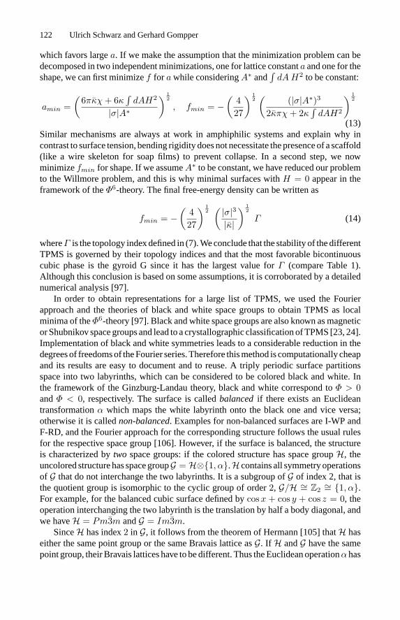
which favors largea. If we make the assumption that the minimization problem can bedecomposed in two independentminimizations, one for lattice constanta and one for theshape, we can first minimizef for awhile consideringA∗ and

∫dAH2 to be constant:

amin =(

6πκχ+ 6κ∫dAH2

|σ|A∗

) 12

, fmin = −(

427

) 12

((|σ|A∗)3

2κπχ+ 2κ∫dAH2

) 12

(13)Similar mechanisms are always at work in amphiphilic systems and explain why incontrast to surface tension, bending rigidity doesnot necessitate thepresenceof a scaffold(like a wire skeleton for soap films) to prevent collapse. In a second step, we nowminimizefmin for shape. If we assumeA∗ to be constant, we have reduced our problemto the Willmore problem, and this is why minimal surfaces withH = 0 appear in theframework of theΦ6-theory. The final free-energy density can be written as

fmin = −(

427

) 12

( |σ|3|κ|

) 12

Γ (14)

whereΓ is the topology indexdefined in (7).Weconclude that thestability of thedifferentTPMS is governed by their topology indices and that the most favorable bicontinuouscubic phase is the gyroid G since it has the largest value forΓ (compare Table 1).Although this conclusion is based on some assumptions, it is corroborated by a detailednumerical analysis [97].

In order to obtain representations for a large list of TPMS, we used the Fourierapproach and the theories of black and white space groups to obtain TPMS as localminima of theΦ6-theory [97]. Black and white space groups are also known asmagneticorShubnikov spacegroupsand lead toa crystallographic classificationof TPMS [23, 24].Implementation of black and white symmetries leads to a considerable reduction in thedegreesof freedomsof theFourier series.Therefore thismethod is computationally cheapand its results are easy to document and to reuse. A triply periodic surface partitionsspace into two labyrinths, which can be considered to be colored black and white. Inthe framework of the Ginzburg-Landau theory, black and white correspond toΦ > 0andΦ < 0, respectively. The surface is calledbalancedif there exists an Euclideantransformationα which maps the white labyrinth onto the black one and vice versa;otherwise it is callednon-balanced. Examples for non-balanced surfaces are I-WP andF-RD, and the Fourier approach for the corresponding structure follows the usual rulesfor the respective space group [106]. However, if the surface is balanced, the structureis characterized bytwo space groups: if the colored structure has space groupH, theuncoloredstructurehasspacegroupG = H⊗{1, α}.H containsall symmetryoperationsof G that do not interchange the two labyrinths. It is a subgroup ofG of index 2, that isthe quotient group is isomorphic to the cyclic group of order2, G/H ∼= Z2 ∼= {1, α}.For example, for the balanced cubic surface defined bycosx + cos y + cos z = 0, theoperation interchanging the two labyrinth is the translation by half a body diagonal, andwe haveH = Pm3m andG = Im3m.

SinceH has index2 in G, it follows from the theorem of Hermann [105] thatH haseither the same point group or the same Bravais lattice asG. If H andG have the samepoint group, their Bravais latticeshave tobedifferent. Thus theEuclideanoperationαhas


to be a translation which extends one cubic Bravais-lattice into another. For the cubicsystem, there are only three different Bravais lattices (simple cubic P, body-centeredcubic I and face-centered cubic F), and only two possibilites to extend one into the otherby a translationtα: for tα = a(x + y + z)/2 a P-lattice becomes a I-lattice, and fortα = ax/2 a F-lattice becomes a P-lattice. The conditionΦ(r + tα) = −Φ(r) leadsto reflection conditions for the reciprocal vectors. For Miller indices(h, k, l), one findsh + k + l = 2n + 1 for P → I, andh, k, l = 2n + 1 for F → P . Note that thesereflection conditions are similar to the well-known onesh + k + l = 2n for I andh + k, h + l, k + l = 2n for F. The P-surface has space groupPm3m, but a black andwhite symmetry with supergroupIm3m, therefore it is an example for the caseP → I.Thus we haveh + k + l = 2n + 1 and the first Fourier mode is(1, 0, 0). Note thatthe double P structure, which one would expect for a diblock copolymer system, has noblack and white symmetry, but space groupIm3m, thus one hash + k + l = 2n andthe first mode is(1, 1, 0).

If H andG have the same Bravais lattice, their point groups have to be different.Thus the Euclidean operationα has to be a point group operation which extends onecubic point group into another one. There are five cubic point groups and six ways toextend one of them into another by somePα. The conditionΦ(Pαr) = −Φ(r) leads tomore complicated rules than in the case of identical points groups [97]. However, thereare few relevant examples from this class, the most interesting one being the gyroid G,wherePα is the inversion and the resulting rules are rather simple again (the even partof the Fourier series vanishes).

Fischer and Koch have completely enumerated all 34 cubic group-subgroup pairsG − H with index 2 which are compatible with cubic balanced TPMS [23]. Althoughthere is no way to completely enumerate all TPMS belonging to a given pairG − Hin general, this is possible for a certain subset, that is for all cubic balanced TPMSwhich contain straight lines which form a three-dimensional network [23]. This listreads P, C(P), D, C(D), S and C(Y). In our work, we implemented Fourier series forthese structures as well as for the gyroid G (which is balanced, but does not contain anystraight lines) and the non-balanced structures I-WP and F-RD. In some cases like G,D and P, the first mode of the Fourier ansatz implementing the correct black and whitesymmetry is already sufficient to obtain a representation which is topologically correct(nodal approximation). In all other cases investigated, the addition of one more mode(with the relative weight fixed by visual inspection) is sufficient. Nodal approximationsfor bicontinuous structures have been discussed first by vonSchnering andNesper [115].In Table 2 and Table 3 we give nodal approximations and the corresponding space groupinformation for some of the balanced and non-balanced structures investigated.

Implementing the complete Fourier series and numerically minimizing theΦ6-functional from (8) with nodal approximations as initial conditions, we arrived atimproved nodal approximationswhich were tabulated in [97] with up to six Fouriermodes. The isosurface construction is easily implemented using the marching cubealgorithm. The resulting triangulations can then be used to investigate geometricalproperties of these surfaces. In particular, widely used mathematics programs (likeMathematica, Maple or Matlab) can be easily used to obtain useful representationsof TPMS from (improved) nodal approximations. Our numerical work shows that the


Table 2.Group - subgroup pairsG −H, the relationH → G between them and nodal approxima-tions for some balanced cubic minimal surfaces.G andH differ either in Bravais lattice or in pointgroup, but not in both. Nodal approximations only consider the space group information given byG − H. For the simple cases, the first mode of the corresponding Fourier series is sufficient toobtain the correct topology.

H G H → G nodal approximations

G I4132 Ia3d 432 → m3m sin(x) cos(y) + sin(y) cos(z) + sin(z) cos(x)D Fd3m Pn3m F → P cos(x− y) cos(z) + sin(x+ y) sin(z)P Pm3m Im3m P → I cos(x) + cos(y) + cos(z)C(P) Pm3m Im3m P → I cos(x) + cos(y) + cos(z) + 3 cos(x) cos(y) cos(z)

Table 3.Nodal approximations for some non-balanced cubicminimal surfaces, for whichH ≡ G.In these cases, more than one mode is needed.

G nodal approximations

I-WP Im3m 2[cos(x) cos(y) + cos(y) cos(z) + cos(z) cos(x)]−[cos(2x) + cos(2y) + cos(2z)]

F-RD Fm3m 4 cos(x) cos(y) cos(z)−[cos(2x) cos(2y) + cos(2y) cos(2z) + cos(2z) cos(2x)]

-40 -30 -20 -10 0

0.02

0.06

0.1

K -150 -125 -100 -75 -50 -25 0

0.1

0.2

0.3

K

(a) (b)

I-WP

D

G

PS

F-RD

C(P)

Fig. 7. Distributionf(K) ofGaussian curvatureK over the cubicminimal surfaces investigated inthe framework of theΦ6-model. (a) For the structure G, D, P and I-WP, the data is obtained fromtheir exact Weierstrass representations; the agreement with the numerical results from theΦ6-model is good (not shown). (b) For the structures F-RD, S and C(P), noWeierstrass representationis known, and the data is obtained from theΦ6-model.

six modes of the improved nodal approximations are sufficient to decrease the devia-tion of the curvature properties from the real TPMS by one order of magnitude com-pared to the nodal approximations. Also we measured for the first time the distributionf(K) =

∫dA(u, v) δ(K − K(u, v)) of Gaussian curvatureK over the surfaces. For

this purpose, we used up to 100 Fourier modes. The distributionsf(K) for differentstructures are plotted in Fig. 7. In the cases for which Weierstrass representations areknown, the same data has been derived from the exact representations, and the resultingagreement was very good. In general, we found that the surfaces C(D), C(P), F-RD, Sand C(Y), for which no Weierstrass representations are known, are much more compli-


cated than the cases G, D, P and I-WP. This is evidenced by larger values of the topologyindexΓ , multi-modal distributionsf(K) of Gaussian curvatureK, and the larger widthsof these distributions. The latter property can be quantified by defining a dimensionlessvariance

∆ =〈(K − 〈K〉)2〉

〈K〉2 (15)

where〈. . . 〉 means area average. In Table 4 we give the variance∆ of the differentdistributions. Its value is the same for G, D and P due to the existence of a Bonnet-transformation between them. Thismeans thatG,DandPhave the narrowest distributionof K (they are most uniformely curved), and all other structures have a considerablywider one, with I-WP being the next best structure.

Table 4. Variance∆ of the distributions of Gaussian curvaturef(K). The values for∆ are thesame for G, D and P due to the existence of a Bonnet-transformation between them.

G, D, P I-WP S F-RD C(P)∆ 0.218702 0.482666 0.586079 0.649801 0.842022

4 Parallel Surfaces

We now consider the case of cubic bicontinuous phases in lipid-water mixtures. Thetwo examples for the experimental phase behavior of such systems given in Fig. 5 showobvious similarities, and we will show now that a theoretical description can nicely ex-plain these [99, 100]. It has been shown by a thorough analysis of electron density mapsderived from X-ray data that the mid-surfaces of the cubic bicontinuous structures inthese systems are very close to minimal surfaces [68]. Indeed if one considers the lipidbilayer as one entity, it has no spontaneous curvature by symmetry and one expects aminimal surface shape for themidsurface. Each of the twomonolayers of the bilayer hasunequal sides and therefore finite spontaneous curvature. For lipids monolayers, spon-taneous curvature increases towards the water side as a linear function of temperature.From the interface point of view, one expects each monolayer to form a CMC-surface.However, then the distance to the minimal mid-surface would vary with position andthe amphiphilic tails would have to stretch in order to fill the internal space of the mem-brane [3, 10]. It can be shown in the framework of a simple microscopic model thatthe relative importance of stretching to bending contributions to the free energy of thebilayer scales as(a/δ)2, wherea is lattice constant andδ is tail length [100]. Thereforestretching is probibitively expensive and the twomonolayers do not formCMC-surfacesas expected from the curvature energy of (1), but rather parallel surfaces to the minimalmid-surface. The free energy of the cubic bicontinuous phases then follows by specify-ing (1) with spontaneous curvature for two monolayers which are parallel surfaces to agiven TPMS. Since the parallel surface geometry does not allow to completely relax thebending energy, the overall structure is calledfrustrated[3, 10, 20].


In principle, the analysis in the framework of the parallel surface model is rathersimple, since there exist exact formulae which express the geometrical properties of theparallel surface as a function of the geometrical properties of the minimal surface:

dAδ = dA (1 +Kδ2) , Hδ =−Kδ

1 +Kδ2 ,Kδ =K

1 +Kδ2 (16)

whereδ is the distance between the two surfaces (that is amphiphilic chain length). Notethat these formulae are an extension of Steiner’s theorem from integral geometry to non-convexbodies,which is validas longas thedistanceδ is smaller than thesmallest radiusofcurvature of the surface (otherwise the surface will self-intersect). Since mean curvatureH vanishes on the reference surface, the bending energy now becomes a function onlyof its Gaussian curvatureK. However, as we have seen above,K is distributed overthe TPMS in a non-trivial way, which makes the detailed analysis rather complicated.Nevertheless, one central conclusion can be already made at this point: using (16) in (1)leads to an effective curvature energy for the lipid bilayer (to second order inδ) [85]

Fbi =∫

dA{4c20δ

2κ+ (2κ+ 8c0δκ+ 4c20δ2κ)K + 4κδ2K2} . (17)

Thus we see that although effective spontaneous curvature vanishes due to the bilayersymmetry, the effective saddle-splay modulus,κbi = 2κ+ 8c0δκ+O(δ2), is correctedto higher positive values due to the presence of the monolayer spontaneous curvaturec0.We conclude that as long asc0δ � −κ/4κ, the bicontinuous cubic phases are favoredover the lamellar phase, since the preferred curvature of the monolayers translates into atopological advantage of saddle-type bilayer structures. We also see that the correctionterm inκbi is linear inc0 and therefore in temperatureT . Therefore bicontinuous phasesbecomemore favorable with increasing temperature in general (compare also Sect. 6 ondisordered bicontinuous structures).

For a detailed analysis of cubic bicontinuous phases made from bilayers, we firstnote that the volume fraction of the lipid tails (the hydrocarbon volume fraction, whichfor simplicity we identify with the lipid volume fraction, since the lipid heads are rathersmall) can be calculated as

v =1a3

∫ δ

−δ

dδ′∫

dAδ′= 2A∗

(δ

a

)+

4π3χ

(δ

a

)3

(18)

where again we have used the Gauss-Bonnet theorem. (18) can be inverted to givea/δ,the lattice constanta in units of the chain lengthδ, as a function of hydrocarbon volumev. For smallv we find

a

δ=

2A∗

v

(1 +

112 Γ 2 v

2 + O(v4))

. (19)

and one can check numerically thata/δ = 2A∗/v is an excellent approximation forv � 0.8. For larger valuesofv, the surfacesbegin to self-intersect andourmodel becomesunphysical. Combining (1) and (16) yields for the bending energy per unit volume ofthe two monolayers (we use a factorδ/4κc20 to write this expression dimensionless anda factorδ to write c0 dimensionless)


f = v{∫

dA∗

A∗

(1 −Ξ(K∗)

( v

Γ

)2)−1

(20)

×(

1 − 1 + c0c0

Ξ(K∗)( v

Γ

)2)2

+r

4c20

( v

Γ

)2 }

whereK∗ = Ka2 is scaled Gaussian curvature,δ/a has been replaced byv/2A∗,Ξ(K∗) has been defined asK∗A∗/8πχ (this can be considered to be a local analogueof Γ 2), andr as−κ/2κ (0 ≤ r ≤ 1 due to the restrictions onκ). The free-energydensityf now is a function of lipid volume fractionv, spontaneous curvaturec0, theratio r of the two bending constants, and the distributionf(K) of Gaussian curvatureK. The (numerical) evaluation of this expression is only possible with the knowledgeof thef(K) for all TPMS of interest, which have been numerically obtained in [97] asdescribed above.

0 0.2 0.4 0.6 0.8 1

0.2

0.6

1.0

1.4

0.48 0.52 0.56

0.065

0.075

v

fP

D G

0 0.2 0.4 0.6 0.8 1

0.2

0.3

0.4

0.1

c0 G

DP

ρW

Lα

(a) (b)

Fig. 8. For cubic bicontinuousphases in lipid-watermixtures, the lipidmonolayers canbemodeledas parallel surfaces to a minimal mid-surface. (a) Free energy densitiesf as a function of lipidvolume fractionv for several cubic bicontinuous phases and the lamellar phase. (b) Theoreticalphase diagram as a function of water volume fraction and (dimensionless) spontaneous curvature.

In the limit of a planar mid-surface (lamellar phase), (20) simplifies tof = v- the larger the lipid volume fraction, the more frustrated bending energy per volumeaccumulates. For a full analysis, one also has to include the effect of thermal fluctuations.For the lamellar phase, they lead to a steric repulsion between the interfaces, which leadto an additional term∼ v3/(1 − v)2 for the lamellar phase. For the cubic bicontinuousphases, steric repulsion is irrelevant since the lateral restriction on the scale of a latticeconstant leadsonly to small perpendicular excursions.However, here the renormalizationof the saddle splay modulusκ becomes relevant, and the formula given in (5) has to beincorporated. The renormalization of bending rigidityκ and spontaneous curvaturec0 isirrelevant here, since thermal fluctuations occur mainly on the level of the lipid bilayer,for which mean curvatureH vanishes. For the lamellar phase, Gaussian curvatureKvanishes as well, and the renormalization of all material parameters is irrelevant. Puttingeverything together, we can numerically calculate phase diagrams from the free energydensities of the different phases by using the Maxwell construction (construction ofconvex hull). In Fig. 8 we show both the free energy densities as a function of lipid


volume fractionv (for fixed spontaneous curvature) and the theoretical phase diagramas a function of water volume fraction and spontaneous curvature. The main results arein excellent agreement with the experimental phase diagram shown in Fig. 5: from themany TPMS considered, only G, D and P are stable, their regions of stability have theshape of shifted parabolae, and they occur in the sequence L - G - D - P -emulsificationfailure. These results can be understood as follows: G, D and P can achieve the leastfrustration since they have the narrowest distribution of Gaussian curvature as measuredby the variance∆ given in Table 4. This prediction has been stated before by Helfrichand Rennschuh [50], but at that time hardly any data was known to support it. The lipidvolume fraction at which they achieve this can be estimated by setting the dimensionlessmean curvature averaged over the parallel surface

〈Hδ〉δδ =∫dAδ Hδδ∫dAδ

=(v/Γ )2

4 − (v/Γ )2(21)

equal to the spontaneous curvaturec0. Thereforec0 as a function ofv essentially scalesas∼ (1 − ρW )2/Γ 2, whereρW = 1 − v is the water volume fraction. This explainsthe characteristic shape of the bicontinuous stability regions in both the theoretical andexperimental phase diagrams. Note that at high temperature, that is large spontaneouscurvature, eventually the hexagonal phase will become stable, which cannot be treatedin the framework presented here. The optimal lipid volume fractionv follows from (21)as

v =(

4c01 + c0

) 12

Γ . (22)

Therefore the structures G, D and P become stable in the sequence of their geometryindexΓ , that is as G - D - P. If the water content corresponds to a average curvature ofP which is larger than the optimal (spontaneous) curvature, some of the water is simplyexpelled from thestructure, inorder tokeep theoptimal curvature (emulsification failure).Finally it should be noted that the Bonnet-transformation connecting G, D and P causesthe three structures to be stable along a triple line (see inset of Fig. 8). This means thatthe stability of D andP is very delicate and can easily be destroyed by additional physicaleffects. Therefore we conclude that in the framework of our interfacial approach, fromall TPMS considered the gyroid G is the only phase which has a robust stability inlipid-water mixtures, since among the phases with favorable distribution of Gaussiancurvature, its geometrical properties are closest to the ones of the lamellar phase.

5 Surfaces of Constant Mean Curvaturve (CMC)

Surfaces of constant mean curvature (CMC-surfaces) haveH = const everywhere, sominimal surfaces are a special case of CMC-surfaces. In contrast to minimal surfaces,CMC-surfaceswith finiteH canbecompact, but theonlyCMC-surfacewhich is compactand embedded is the sphere (for a long time, the sphere was believed to be the onlycompact CMC-surface, but in 1986 Wente found the first CMC-torus). Non-compactembedded CMC-surfaces are cylinder and unduloid, and all other known CMC-surfacesare doubly or triply periodic.


0.2 0.4 0.6 0.8

-4

-2

0

2

4

v

H*

(b)0.2 0.4 0.6 0.8

2

3

4

A

v

*

(a)

G

D

P

I-WP

F-RD

C(P)

C(P)

F-RDG

D

P I-WP

Fig. 9. Geometrical data for triply periodic surfaces of constant mean curvature: (a) scaled surfaceareaA∗ and (b) scaled mean curvatureH∗ as a function of volume fractionv. The two branchesare symmetrical for G, D, P and C(P) since their minimal surface members are balanced.

CMC-surfaces are solutions to the variational problem of minimal surface area un-der a volume constraint. This can be shown as follows: we first introduce a Lagrangeparameter for volume, that is pressurep. The corresponding energy is−pV . For normalvariationsδφ(u, v), wehave∆F = 2δσ

∫dAφ(u, v)H(u, v)−pδ

∫dAφ(u, v)+O(δ2).

If the surface is required to be stationary in regard to variations inδ, weobtain theLaplaceequationH = p/2σ andH is constant over the whole surface. This explains why soapbubbles and liquid droplets are spheres (respectively spherical caps when bound by asurface). In amphiphilic systems, CMC-surface arise in the presence of spontaneouscurvature: like minimal surfaces minimize the Willmore functional

∫dAH2, CMC-

surfaces withH = c0 minimize the functional∫dA(H − c0)2. In any case, sinceH is

constant over the surface, surface area and volume now vary in the same way, and wehavedA/dV = 2H.

Table 5. Values forc = dv(H∗)/dH∗|H∗=0, wherev(H∗) is the volume fraction of one of thetwo labyrinths for the corresponding family of surfaces of constant mean curvature. Themeasuredvalues follow from our spline interpolation of the numerical data of [2]. In the second row we give−A0

2/2πχ, a new estimate forc derived in the text.

G D I-WP P F-RD C(P)measured 0.21910.14110.13850.21170.06650.0466approximation0.19010.14650.15920.21880.09060.1226

All simple TPMSwhich are of interest for physical reasons are members of a familyof CMC-surfaces [55]. Each of these families consists of two branches, correspondingto positive and negative mean curvatures, which are separated by the minimal surfacemember. Like theminimal surfacemember, each of the the triply periodic CMC-surfacesof the family partitions space into two intertwined, yet separate labyrinths, with volumefractionsv and1−v. Each family ofCMC-surfaces, and therefore the volume fractionsofthe two labyrinths and the surface areaA, is parametrized byH. If the TPMS-memberis balanced, then the operationα maps one branch of the family onto the other, in


particularv(H) = 1 − v(−H), v(H = 0) = v0 = 0.5 andA(H) = A(−H). For anamphiphilic monolayer of thicknessδ in a ternary system,v can be identified with thehydrocarbon volume fraction (that is oil and amphiphilic tails),1 − v with the watervolume fraction (where we neglect the contributions of the amphiphilic heads), and2Aδwith the amphiphile volume fraction. In the seminal work by Anderson, Davis, NitscheandSciven from1990, theCMC-familieswerenumerically constructed forP,D, I-WP,F-RDandC(P) using finite elementmethods [2]. In 1997,Grosse-Brauckmannnumericallyconstructed the G-family in a similar way (using the software packageSurface Evolver)[44]. For these families, the following data has been tabulated: volume fractionv as afunction of scaled mean curvatureH∗ and scaled surface areaA∗ as a function ofv.Rearrangement and interpolation with cubic splines provides smooth functionsH∗(v)andA∗(v). As v is varied away from the valuev0 for the TPMS (= 0.5 for balancedstructures), one has

H∗(v) = − (v − v0)c

+ O ((v − v0)2

)(23)

A∗(v) = A0 − (v − v0)2

c+ O (

(v − v0)3)

where the numerical value ofc can beextracted from the cubic splines (compareTable 5).Note that the two relationships are not independent due to the relationdA/dV = 2H.They are related throughc, whose values are well approximated by the analogous valuesfor the parallel surface companions to the TPMS, which can be derived as follows[98]: if δ denotes the perpendicular distance from the minimal to its parallel surface, tolowest order inδ the volume fractionv and the mean curvatureH∗, averaged over thesurface in the unit cell, are given byv = v0 + A∗δ andH∗ = 2πχδ/A∗, respectively.ThusH∗ = 2πχ(v − v0)/A∗2 andc = −A∗2/2πχ for the parallel surface case. Thecorresponding numbers are given in Table 5; except for C(P), the overall agreement withthe numerical data forc for the CMC-surfaces is remarkably good.

Equation (23) is a useful approximation for CMC-surfaces close to the TPMS, wheretheybehavesimilar toparallel surfaces.However, asmeancurvaturegrows, thenumericaldata starts to deviate from these approximations, changes inv andA∗ become slower,and a turning point is reached, wherev reaches an extremal value and starts to decreaseagain as a function ofH. Beyond the turning point, the surfaces correspond to nearlyspherical regions connected by small necks which resemble pieces of unduloids. Finallythese necks disappear and each branch terminates in an assembly of sphere, whichmightbe close-packed or self-intersecting. Figure fig:cmc shows the geometrical data for thefamilies G, D, P, C(P), I-WP, F-RD as tabulated in the literature [2, 44]. We do not showthe parts of the data beyond the turning point, as these correspond to surfaces whosestructure is unphysical.

We now consider a ternary mixture of water, oil and amphiphile, where amphiphilesself-assemble into monolayers with spontaneous curvaturec0. In such a system, allrelevant phases (micellar, hexagonal, lamellar, cubic bicontinuous) can be modeled asCMC-surfaces (spheres, cylinders, planes, triply periodicCMC-surfaces). This approachhas first been used bySafran and coworkers [94, 95, 116], who in particular discussed thesurfaces from the D-family. In our work [98], we extended this analysis to all families ofinterest, including the G-family, for which the relevant data has become available only


recently andwhich features very prominently in experimental systems.A ternarymixturehas two independent degrees of freedom for concentration, which we choose to be thehydrocarbon volume fractionv and the ratiow of amphiphile to hydrocarbon volumefraction. For the formulae given later it is in fact useful to modify the definition ofw andto scale it with the dimensionless spontaneous curvaturec0:w = ρA/vc0δ. The analysisof (1) for CMC-surfaces is simplified considerably by the fact that as mean curvatureHis constant, there is no difference between local and global curvature properties and theintegral over the surface becomes trivial. We use a factor2κc30 to rewrite the free-energydensity in the dimensionless form

f =A

c0V

(H

c0− 1

)2

− 2πχrc03V

. (24)

For phases with lamellar, cylindrical and spherical aggregates, this free-energy densitycan easily be expressed as a function of the concentration degrees of freedom:

fL(w, v) = wv, (25)

fC(w, v) = wv(w

4− 1

)2, (26)

fS(w, v, r) = wv

[(w3

− 1)2

− rw2

9

]. (27)

Note that onlyfS depends onr, since the other two structures have no Gaussian curva-ture. Since the aggregates are disconnected, the dependence onv is trivial. The phaseboundariesS −C, S −L,C −L and the emulsification failure are obtained from (25),(26) and (27) to bew = 24/(7 − 16r), w = 6/(1 − r), w = 8 andw = 3/(r − 1),respectively. For example, forr = 0 and increasingw, we find the phase sequence L -C - S -emulsification failure, which is typical for amphiphilic systems (for simplicity,we identify phase transitions with crossing points of the free-energy-density curves, anduse the Maxwell construction only for the emulsification failure). In Fig. 4 one seesthat experimentally the emulsification failure indeed occurs at constantw (straight linethrough water apex). For increasingr, the spherical phase becomes more favorable andfinally supresses the cylindrical phase.

The structures based on CMC-surfaces discussed here are very different from thelipid bilayer structures discussed in the preceding section: now only one monolayeris present, and one of the two labyrinths is filled with hydrocarbon. In the following,they are calledsingle structures. It should be noted that for non-balanced structures, itmakes a difference which of the two labyrinth is filled with hydrocarbon; for example,the I-WP-family generates two single structures, which we call I and WP. In ternaryamphiphilic systems there also exists an analogue to the bilayer structures discussedbefore, which we calldouble structuresand mark with an indexI. Double structureshave the same geometries like cubic bicontinuous phases in diblock copolymer systems.They can be considered to be TPMS-based bilayer structures where the inner part of thebilayer has been swollen with suitable solvent. Since each of the twomonolayers has thesame spontaneous curvaturec0, a double structure can be modeled as the combinationof the two surfaces of a CMC-family withH = c0 andH = −c0. Since for not too large


H these two CMC-surfaces essentially correspond to the shrinkage of one of the twoseparate labyrinthsdefinedby theminimal surfacemember, the two interfacesof adoublestructure do not intersect. Note that in principle there exists another class of structures,that is double structures where oil and water (and therefore amphiphile orientation andmean curvature) have been reversed. However, since finite spontaneous curvature selectsonly phases with curvature towards one specific side, they are suppressed for energeticreasons by the lamellar phase.

In our work [98], we considered 8 different single structures, which exist forthe volume intervals[0.056, 0.944] for G, [0.131, 0.869] for D, [0.249, 0.751] for P,[0.481, 0.519] for C(P),[0.357, 0.857] for I, [0.143, 0.643] for WP, [0.439, 0.625] for Fand[0.375, 0.561] for RD. We also considered 6 double structures, which exist for thevolume intervals[0.112, 1.0] for GI , [0.262, 1.0] for DI , [0.498, 1.0] for PI , [0.962, 1.0]for C(P)I , [0.624, 1.0] for I-WPI and[0.818, 1.0] for F-RDI . Note that the gyroid struc-tures cover the largest intervals inv for their respective class: there is no other structurewhich can incorporate so extreme volume fractions like the gyroid. Together with the3 non-cubic phases treated above, we considered 17 different phases. Since the cu-bic phases consist of one connected aggregate, the scaling of the free energy densityf with hydrocarbon volume fractionv will be non-trivial. For a given value ofv, themean curvatureH(v, a) = H∗(v)/a and the surface areaA(v, a) = A∗(v)a2 within aunit cell are determined by the curves plotted in Fig. 9. The amphiphile concentrationρA = A(v, a)/a3 = A∗(v)/a fixesa, so thata = A∗(v)/ρA = A∗(v)/(wvc0). From(24) we can then derive

fBC(w, v, r) = wv [Λ(v) wv − 1]2 + r(wv)3

Γ (v)2(28)

where we have used the definition for the curvature indexΛ and the topology indexΓfrom (7). Note that now the indices arev-dependent. For the single structures,f followsby combining using the data shown in Fig. 9 with the definitions in (7). For the doublestructures, the procedure is somehow more complicated. However, for balanced doublestructures, it becomes simple again, one then can use

ΛI(v) = Λ(v/2)/2, ΓI(v) = 2Γ (v/2), fBC,I(w, v, r) = 2fBC(w,v

2, r) (29)

in (28).For r = 0 (vanishing saddle splay modulusκ), the analysis of cubic bicontinuous

phase behavior becomes rather simple: in contrast to the case of the parallel surfacemodel discussed in the last section, now the bending energy given in (28) can be com-pletely relaxed, namely by satisfyingw(v) = 1/vΛ(v). This leads to lines of vanishingfrustration in the Gibbs triangle. For the free-energy density of the micellar and hexag-onal phases ((27) and (26), respectively), the lines of vanishing frustration follow asw = 3 andw = 4, respectively. All lines of vanishing frustration are plotted in Fig. 10a.Obviously for this case phase behavior is very complex and degenerated, since everystructure considered has some region of stability around its line of vanishing frustration.This type of degeneracy caused by the bending energy has been discussed before [6] andleads to the conclusion that additional physical effects have to be operative, as it is notobserved in experimental systems.


W O

A

S

C

QIQ

W O

A

(a) (b)

C

S

EF

L

G

G

I

Fig. 10. (a) Lines of vanishing frustration forr = 0. With increasing amphiphile concentration,the structures S - C- double cubic - single cubic are stable. (b) Phase behavior forr = 1/15.Now all cubic phases have been supressed except the two gyroid phases. In (a) and (b),c0 = 1/6,which corresponds toH2O/C14/C12E5 atT = 20◦C.

Using (23), a simple approximation can be derived for the lines of vanishing frus-tration of the cubic phases:

w = −cA0/v0(v − v0), wI = −4cA0/(v − 1) . (30)

Thus the minimal surface case corresponds to the stable solutions forw � 1 atv = v0andv = 1, respectively. For the balanced single structures and the double structuresthe hierarchy of the different phases within the band-like region occupied by a certainstructural type is thus determined by the values ofcA0. Using the approximationc ≈−A∗2/2πχ derived above, we findcA∗ ≈ Γ 2, whereA∗ andΓ correspond to theminimal surface members. Therefore the phase sequence is approximately determinedby the topology index of the minimal-surface member of each family. In particular, fora given structural type we expect to find the sequence G - D - P as afunction of eithervorw.

Forr > 0 (negative saddle splay modulusκ), spheres becomemore favorable, cubicphases less favorable and cylinders and lamellae experience no change in free energy.Therefore the cubic phases will finally disappear, but our numerical analysis shows thatcubic phases can persist up tor = 0.2, in contrast to earlier work, which predictedr = 0.1 [116]. The reason for this becomes clear in Fig. 10b where we show the fullphase diagram forr = 1/15 = 0.07: the only cubic phases stable here are the two gyroidstructures, which have not been considered before. There are two main reasons for theiroutstanding performance: (28) shows that their large values for the topology indexΓreduces the energetic penalty caused byr, and since they can accomodate extremevolume fractions, they can compete with other structures at all relevant concentrations.By comparing the theoretical phase diagram fromFig. 10with the experimental one fromFig. 5, we conclude that the experimental system should correspond to a rather largevalue ofr. Earlier work moreover suggests that incorporation of thermal fluctuations


would favormicellar phases near thewater-amphiphilic side and lamellar phases near thewater apex [101]. Suchamodification is expected to considerably improve theagreementbetween the two phase diagrams.

6 Random Surfaces

6.1 Microemulsion and Sponge Phases

Whenκ/kBT , the bending rigidity in thermal units, becomes sufficiently low (that istemperatureT sufficiently high), bicontinuous structures can now longer maintain theirlong-range crystalline order and melt into a disordered phase, which is characterized byan exponential decay of correlations in the interfacial positions. Such phases have beenobservedexperimentally for a long time inmanybinary and ternary amphiphilic systems.Microemulsionsare macroscopically homogeneous and optically isotropic mixtures ofoil, water and amphiphiles. On a mesoscopic scale, they consist of two multiply con-nected and intertwined networks of oil- and water-channels, which are separated by anamphiphilic monolayers. Free-fracture microscopy, where the sample is quickly frozen,cut, and then studied with an electron microscope, reveals the intriguing structure of thisphase [52], see Fig. 11. A similar phase, thesponge phase, appears in binary systems ofwater and amphiphile, where now the two labyrinths are occupied by water, which areseparated by an amphiphilic bilayer. The pictures obtained by free-fracture microscopy[107] are evenmore suggestive in this case, because the sample has a preference to breakalong the bilayer mid-surface, so that the three-dimensional structure of the membranebecomes visible. An example is shown in Fig. 12, which clearly shows the saddle-likegeometry of the amphiphile film. Therefore, the intuitive picture of microemulsion andsponge phases as fluid versions of bicontinuous cubic phases is strongly supported bythese experiments.

These phases have been investigated experimentally in considerable detail overmanyyears. In particular, their phasebehavior and scattering intensities havebeenstudied care-fully. A theoretical understanding of the statistical mechanics of membranes, however,is only beginning to emerge in recent years [75, 40, 78, 18, 35]. This is no surprise, sincethe statistical mechanics of a surface, which can not only change its shape, but also itstopology in all possible ways, is extremely complicated. In principle, a partition functionof the form

Z =∑

topologies

∫ ′DR(τ) exp{H[R(τ)]/kBT} (31)

has to be calculated, whereDR(τ) denotes an integration over all possible shapes withparametrizationR(τ) of the surface at fixed topology, whereτ is a two-dimensionalcoordinate system on the surface. However, this integral cannot be just over all possibleparametrizationR(τ) of a surface of fixed topology, but has to be restricted to thoseparametrizations, which lead to physically different shapes in the embedding space; thisis indicated by the prime. Finally, the contributions off all different topologies have to besummed over. It is clear that this problem is sufficiently complex that no exact solutionwill be found anytime soon. Therefore, approximations have to be made in order to getsome insight into the behavior of these phases.


Fig. 11. Freeze-fracture microscopy picture of a balanced microemulsion phase. From [52].

Fig. 12. Freeze-fracture microscopy picture of a sponge phase. From [107].


6.2 Gaussian Random Fields

A very useful approach is to describe the interfaces as isosurfaces ofGaussian randomfields(GRF). This corresponds to a Ginzburg-Landau model as discussed in Sect. 2.2,in which the free-energy functional is taken to be quadratic in the scalar fieldΦ(r). ThisGibbs distribution is homogeneous and isotropic, and all the functional integrals areGaussian and can be performed exactly. In fact, there is a considerable mathematicalliteratureon the isosurfacesofGRF,seee.g. thebookbyAdler [1]. Inorder tocomplywiththe conventions of this field, we nowmake two changes to our notation. In the following,area content is denoted byS (rather than byA) and amphiphilic (hydrocarbon) volumefraction byΨ (rather than byv).

Theamphiphilicmonolayers inmicroemulsionshavebeenmodelled as level surfacesof GRF by Berk [4, 5], Teubner [112], Pieruschka and Marcelja [81], and Pieruschkaand Safran [82, 83]. Here the starting point is a Gaussian free-energy functional of thegeneral form

H0[φ] =12

∫d3q ν(q)−1Φ(q)Φ(−q) . (32)

The average geometry of theΦ(q) = α level surfaces can be calculated for arbitraryspectral densityν(q). For the surface density,S/V , the mean curvatureH, the GaussiancurvatureK, and the mean curvature squaredH2, the following averages are obtained[112]:

S

V=

2π

exp[−α2

2

]√13〈q2〉 , (33)

〈K〉 = −16〈q2〉(1 − α2) , (34)

〈H〉 =12α

√π

6〈q2〉 , (35)

〈H2〉 = 〈K〉 +15

〈q4〉〈q2〉 (36)

where

〈qn〉 =∫

d3q

(2π)3qnν(q) . (37)

The valueα of the level cut can be used to describe the preferred curvature of themembrane, as well as the volume fractions of oil and water. Since〈H〉 is a linearfunction ofα, compare (35), this parameter is proportional to the spontaneous curvaturec0. In particular, forα = 0 the mean curvature of the surface vanishes; this applies to abalanced system, wherec0 = 0.

For balanced systems, it follows from (33,34) that the topology indexΓ =√

8/π =0.9003 (compare (7)). This value is only slightly larger than the ones for cubic bicon-tinuous phases (compare Table 1), since the balanced random sponge features only fewdisconnected parts (note thatΓ doubles when the structure is duplicated). For smallcurvatures (that is smallα), one can use (33,34,35) to derive a relationship between


topology indexΓ and curvature indexΛ which is independent of spectral densityν(q)andα:

Γ =√

8π

(1 +

28

π6Λ4 + . . .

). (38)

When the curvature indexΛ increases since the sponge’s interfaces gain curvature, thetopology index increases, too, since disconnected parts proliferate.

TheGFF-approach ismost predictivewhen theGaussianmodel of random interfacesis related to the statistical mechanics of membranes by a variational approximation[82, 83]. In this case, the spectral densityν(q) in the functional (32) is determinedby the requirement that theφ(r) = 0 level surfaces mimic the behavior of interfacescontrolled by the curvature Hamiltonian (1) as close as possible. The usual variationalapproach employs the Feynman-Bogoljubov inequality,

F ≤ F0 + 〈H − H0〉0 (39)

whereH andF are the Hamiltonian and the free energy of the system of interest,respectively, andH0 andF0 the same quantities of the reference system. In this way, anupper bound for the true free energy is obtained. This is more complicated in the case ofrandom surfaces, because the GRF-Hamiltonian is defined everywhere in space, whilethe curvature Hamiltonian is only defined on the level surface. Therefore, the curvatureenergy does not restrict fluctuations of the fieldΦ(r)away from the level surface. In orderto suppress such fluctuations, one usuallymakes themean-spherical approximation, thatis the constraint〈Φ(r)2〉 = 1 is introduced.

With this variational approach, Pieruschka and Safran [82] have been able to derivethe following form for the spectral density

ν(q) =a

q4 + bq2 + c(40)

and to relate the parametersa, b andc to the curvature elastic moduliκ andκ and thesurface densityS/V . The first interesting result is that the spectral density is found to beindependentof κ. Exact expressions for the parameters can be found in [22]. To leadingorder inkBT/κ, the parameters simplify to

a =15π2

16kBT

κ

S

V, (41)

b =32π2

(S

V

)2

, (42)

c =(

3π2

4

)2 (S

V

)4

. (43)

The spectral density (40) is equivalent to the scattering intensity in bulk contrast. ItsFourier transform yields the correlation function

〈Φ(r)Φ(r′)〉 =∫

d3q eiq·(r−r′)ν(q) =A

rexp[−r/ξ] sin(kr) (44)


where the second equality holds for|b| < 2√c. Thus, the correlation function is char-

acterized by two length scales, the correlation lengthξ and the typical domain sized = 2π/k of the oil- of water channels, which are obtained from (40) and (44) to be[113]

ξ−1 =12

√2√c+ b , (45)

k =12

√2√c− b . (46)

With the results (41), (42) and (43), the asymptotic behavior for smallkBT/κ of thedimensionless productkξ is found to be

kξ =64

5√

3κ

kBT. (47)

The free energy of the sponge phase can also be calculated from the GRF approach. Toleading order in an expansion inkBT/κ, the free-energy densityf = F/V is found tobe [83]

f =π2

40[2κ− 5κ]

(S

V

)3

− kBT

12ln

(δS

V

). (48)

This implies that for small membrane volume fractionsΨ = δS/V (where againδ isthe thickness of the amphiphilic interface), the entropic term dominates over the energyterm, and that the sponge phase becomes unstable in this regime.

Wewant to end this sectionwith a short discussion of the reliability of the predictionsof the GRF model as a variational approximation for membrane ensembles. The weakpoint of this approach is that it is not clear whether the calculated entropy is actuallyequivalent to the physical conformational entropy of the membranes [74]. The mainproblem is that the curvature energy only controls the shape of theΦ(r) = 0 levelsurface, while the values of the scalar fieldΦ at all other points in space are not affectedby it. The fluctuations ofΦ in these oil- and water-regions are mainly determined bythe mean-spherical constraint〈Φ2(r)〉 = 1. Obviously, an appreciable contribution tothe total entropy arises from the fluctuations ofΦ these ‘bulk’ regions. This would notaffect the predictions of the model as long as the ‘bulk’ contributions were independentof the interface positions. Unfortunately, there is no argument so far that this is indeedthe case.

6.3 Phase Behavior of Random Surfaces

From here onwe consider only the case of vanishing spontaneous curvature,c0 = 0, thatis balanced microemulsions and sponge phases. Then the phase behavior is controlledby the bending rigidityκ, the saddle-splay modulusκ, the density of membrane area pervolume,S/V , and a microscopic cutoffδ, which can be identified with the thickness ofthe amphiphilic interface. It is very important to realize that for vanishing spontaneouscurvature, phase transition as a function of the amphiphile volume fraction cannot beunderstoodon thebasisof thecurvatureenergyalone—i.e.without considering theeffect


of thermal fluctuations [85]. The reason is that the curvature Hamiltonian is conformallyinvariant in three spatial dimensions, which implies in particular that it is invariantunder a simultaneous rescaling of all length scales. Since the curvature energy is scaleinvariant, the energydensityscales as the third power of an inverse length, i.e. as(S/V )3.Therefore, the curvature energy of any given structure—spherical, cylindrical, lamellar,cubic, or random— scales in exactly the same way with decreasing amphiphile volumefraction, and their relative order ismaintained. Therefore, thermal fluctuations are crucialfor these phase transitions.

It has been suggested by several authors [93, 9, 73, 28] that the free energy of thesponge phase can be obtained by integrating out the membrane fluctuations on scalesless than the typical domain size. This integration over small-scale fluctuations leads torenormalized, scale-dependent curvaturemoduliκR(l) andκR(l) as given by (4) and (5),respectively, withl/δ = Ψ−1, whereΨ is the membrane volume fraction. This impliesthat the curvature Hamiltonian (2) has to be replaced by

F =∫

dA

{12κ+,R(Ψ−1)(k1 + k2)2 +

12κ−,R(Ψ−1)(k1 − k2)2

}(49)

with

κ+,R(Ψ−1) = κ+ +kBT

3πlnΨ , (50)

κ−,R(Ψ−1) = κ− +5kBT

12πlnΨ . (51)

The stability arguments used in Sect. 2.1 imply thatκ+,R andκ−,R have to be positivefor the free energy (49) to be stable against collapse of the structure to molecular scales.Therefore, there are instabilities atκ+,R(Ψ−1) = 0 andκ−,R(Ψ−1) = 0. The latterinstability can be identified with the emulsification failure of the sponge phase, so thatthe phase boundary is predicted to occur at [73]

lnΨ =6π5

κ

kBT. (52)

This result can be understood intuitively as follows. For sufficiently large membranevolume fraction, bothκ+,R andκ−,R arepositive.Therefore, thesystem tries tominimize(k1 + k2)2 and(k1 − k2)2. This can be achieved by decreasing bothk1 andk2, i.e. byswelling a given structure asmuch as possible— the lamellar or sponge phase is stable atthis valueofΨ .On theotherhand, assoonasκ+,R orκ−,R becomenegativeat somesmallvalue ofΨ , the free energy can be reduced by collapsing the structure. With decreasinglength, however,κ+,R andκ−,R increase and finally become positive. Therefore, thecollapse stops at a length scale which is exactly the length scale determined by (52).

It is worth mentioning that a similar result follows from the calculation of the shapesand free energies of passages in lamellar phases [31]. Passages are catenoid-like connec-tions betweenadjacent lamellaewhich proliferate close to phase transitions to disorderedbicontinuous phases. From a detailed calculation, which takes into account the Gaussianmembrane fluctuations, the density,ρ, of passages per unit base area of the stack can beobtained to be


ρ =A0(κ/kBT )

δ2

(d

δ

)4/3

exp[4πκ/kBT ] (53)

Here,A0(κ/kBT ) is a function which has to be calculated numerically; it is predictedto increase monotonically with decreasingκ/kBT in [31]. Therefore, the density ofpassages increases with increasing lamellar spacingd/δ = Ψ−1. When the averagedistance between passages shrinks to the average membrane separation, a transition tothe sponge phase can be expected to occur. This happens at

103

lnΨ/Ψ∗ = 4πκ

kBT(54)

whereΨ∗ is a function ofκ/kBT . Equations (52) and (54) agree perfectly.The consideration of the renormalization ofκ and κ implies that the free-energy

density,f , of the sponge phase should behave as [89, 87, 90]

f = (A+B lnΨ)Ψ3 . (55)

As explained above, the overall scaling withΨ3 derives from the conformal invarianceof the curvature energy.A represents the bending energy without thermal fluctuations,and is a linear function of bothκ andκ. B represents the logarithmic corrections fromthe renormalization and is a linear function of temperature. BothA andB depend on thedetailed geometrical structure of the sponge phase, and thus cannot be obtained fromsimple scaling arguments. It is important to note that the functional dependence of thefree energy (55), which is based on the renormalization of the curvature elastic modulidue tosmall-scalemembrane fluctuations, does not agree with the free energy (48) oftheGaussian random fieldmodel, which includes the topological entropy of a disorderedbicontinuous phase.

6.4 Monte Carlo Simulations of Triangulated Surfaces

In order to go beyond the approximations discussed in Sects. 6.2 and 6.3, discretizedsurface models can be investigated by Monte Carlo simulations [35, 34, 36, 37]. Surfacetriangulations provide the bestwayof discretizing a surface as uniformly as possible. Themodel consists of vertices, which are connected by bonds in such a way that the bondsform a triangular network. Several Hamiltonians have been suggested for triangulatedsurfaces, such that their shapes and fluctuations are governed in the continuum limitby the curvature energy from (1) [35]. Two examples are Gaussian-spring models, inwhich neighboring vertices— the vertices connected by bonds— interact with harmonicspring potentials, and tether-and-bead models, in which the interactionV (r) betweenneighboring vertices is defined the potential

V (r) =

∞ 0 ≤ r < σ00 for σ0 < r < B0∞ B0 < r

(56)

whereσ0 is the hard-core diameter of the beads, andB0 is the tether length. For tetherlengthsB0 <

√3σ0, the network is self-avoiding, because a bead of some distant part of


the membrane does not fit through the hole between the three beads of a triangle, evenfor maximally stretched tethers.

A Monte Carlo simulation of sponge phases requires three types of Monte Carlomoves [36]. The first step is to displace selected beads by a random vector chosenuniformly in the cube[−s, s]3. Here,s is determined by the criterion that roughly50%of trial moves is accepted according to the Boltzmann weight. The second step is tovary the connectivity of the bond network, in order to allow for diffusion and fluidity ofthe membrane. This dynamic triangulation is performed for any two adjacent triangles.The bond which forms the common edge of the two triangles is cut, and a new bond isinserted,which connects the twopreviously unconnectedbeads. Thebondcanonly becutif every bead retains bonds to at least three other beads. This procedure guarantees thatthe network remains two-dimensionally connected, no holes open up in the network,and the topology of the network does not change. Finally, the third step is to changethe topology of the surface. This is done by removing two nearby triangles from thesurface, and by connecting the corresponding vertices by a prism of six new triangles.Of course, the inverse step is also possible, with a passage six triangles being removed,and two new triangles inserted to close the surfaces. The acceptance of both the bond-flip and topology-changemoves is determined by the Boltzmann weight and is thereforecontrolled by the curvature energy. We want to mention parenthetically that some carehas to be taken to find a good discretization of the bending energy [33].

A typical configuration of a triangulated surface in a cubic box with parametersκ, κandΨ chosen in the stability region of the microemulsion or sponge phase is shown inFig. 13. This configuration nicely demonstrates the bicontinuous structure of balancedmicroemulsions and sponge phases. The saddle-like geometry of themembrane can alsobe easily seen. Finally, the figure shows thatlocally the structure of the sponge phasestrongly resembles the cubic phases discussed above. Therefore, a sponge phase shouldindeed be considered as the molten state of the crystalline cubic phase.

A more quantitative comparison with the theoretical approaches of Sects. 6.2 and6.3 above can be made by determining the phase diagram of the randomly-triangulatedsurfacemodel, and by calculating the osmotic pressure,p, in the simulations as a functionof the membrane volume fractionΨ . From (55), we obtain

pδ3/kBT ≡ 1kBT

[Ψ∂f/∂Ψ − f ]

= [(2A+B) + 2B lnΨ ]Ψ3 (57)

i.e. the same functional dependence as the free-energy density itself. This dependenceof the osmotic pressure is indeed nicely confirmed by the simulation data [36]. Thesimulations therefore provide strong evidence for the renormalization of the elasticmoduli of the curvature model and for the dependence (55) of the free energy on themembrane volume fraction.

The phase diagram for fixed bending rigidityκ is shown as a function ofκ andΨin Fig. 14. The simulation data are compared with the prediction (52) for the phaseboundary. Since the slopes of the phase boundaries in this logarithmic plot agree verywell, not only the exponential dependence of the membrane volume fraction at thetransition on the saddle splay modulus is confirmed, but also the value of the universalprefactor in (52) is strongly supported.


Fig. 13. A typical membrane configuration in a sponge phase for bending rigidityκ/kBT � 1.6.The two sides of the membrane are shaded differently in order to emphasize the bicontinuousstructure of this phase. From [36].

1.0

-1 -0.8

0.8

-0.6

0.6

-0.4

0.4

-0.2

0.2

0.3

lamellar

sponge

emulsificationfailure

κ

φ

Fig. 14. The phase diagram as a function of membrane volume fractionΦ and saddle-splaymodulusκ, for bending rigidityκ/kBT � 1.6. Note the logarithmic scale of the abscissa. Thedashed line shows the theoretical prediction (52). From [36].


6.5 Comparison with Experiments

Experimentally, phase diagrams and scattering intensities have been studied system-atically for many different surfactant molecules. Qualitatively, the agreement with thetheoretical approaches is very reasonable. For example, the scattering curve in bulk con-trast shows a peak at non-zero wave vector in the microemulsion phase, which movesout and decreaeses in height with increasing surfactant concentration. A quantitativecomparison, however, is much more difficult. We want to discuss here three differentclasses of experiments, where a such a quantitative comparison has been made.

The first type of experiments are scattering studies in bulk and film contrast. In bulkcontrast, the scattering intensitySww(q) is proportional to the spectral densityν(q) ofthe Gaussian random field model, compare (40), for wave vectorsq which are not muchlarger than the characteristic wave vectork of the domain structure, compare (46). Thefunctional dependence of (40) describes the scattering data in this regime very well,as was first noted by Teubner and Strey [113], who derived this result on the basis of aGinzburg-Landaumodel, very similar to that introduced in Sect. 2.2.Wewant tomentionparenthetically, that for wave vectorsk � q � 1/δ, the intensity is dominated by thescattering from sharp, planar interfaces; in this limit, the famous Podod law [84, 112]predictsI(q) ∼ (S/V )q−4.

In the limit of wave vectorq → 0, the scattering intensity in film contrast is givenby [87]

I(q → 0) ∼ Ψ

(∂p

∂Ψ

)−1

(58)

wherep is the osmotic pressure of (57). For the free energy (55), this implies

[ΨI(q → 0)]−1 ∼ const+ lnΨ (59)

Such a behavior has indeed be observed experimentally in [87]. However, this resulthas been questioned by Daicic et al. [14, 13]. This has lead to a intensive debate, witharguments against [15, 16] and in favor [91, 86] of the existence of a logarithmic renor-malization of elastic moduli in the sponge phase.

In a second type of experiment, information about the average geometry of thesurfactant film can be extracted from the scattering intensity in the regimek < q � 1/δ.This information is contained in the corrections to the asymptotic1/q4 law for smallervalues of thewave vector [111]. Experimentally, the averageGaussian curvature is foundto be [11]

(V/S)2〈K〉 = 1.25 ± 0.10 (60)

which is in excellent agreement with the Gaussian random field result(V/S)2〈K〉 =1/Γ 2 = −π2/8 = 1.23 and simulations of theΦ6-Ginzburg-Landau model [32, 30].

The third type of experiment concerns the phase behavior of mixtures of waterand non-ionic surfactant as a function of temperature and surfactant concentration. Asmentioned in Sect. 4, the saddle-splay modulusκ is a linear function of temperaturein this case. Therefore, the concentrations at the phase boundaries of the lamellar andthe sponge phase are expected from (52) to depend exponentially on temperature. Alogarithmic plot of the phase diagram ofC12E5 in water [109], compare Fig. 4, isindeed consistent with this expectation.


The most detailed information about both the scattering intensities and phase be-havior in these systems has been obtained very recently in ternary amphiphilic systemsof water, oil and non-ionic surfactantCiEj , to which small traces of an amphiphilicblock copolymer has been added [53, 21, 22, 29, 38]. The results obtained in this systemprovide further, strong evidence for the existence of a logarithmic renormalization ofκandκ in microemulsions and sponge phases.

7 Summary and Outlook

In this contribution we discussed the geometrical properties of surfaces which can beused as structural models for cubic bicontinuous phases in amphiphilic systems: triplyperiodic minimal surfaces, their parallel surfaces and constant mean curvature compan-ions, and bicontinuous random surfaces. For each class of surfaces, we showed how thegeometrical properties translate into physical properties of bicontinuous phases in am-phiphilic systems in the framework of an interfacial description. The surprising successof this approach relates to the fact that in amphiphilic systems, the solvent has little phys-ical properties by itself and the free energy is essentially determined by the interfaces.Although there are several physical effects which have been neglected in our treatmentof amphiphilic systems, including van der Waals and electostatic interactions, it can beconcluded that the most essential aspects of phase behavior are now well understood interms of the properties of the underlying geometries.

During the last years, the interest in bicontinuous phases has increased due to somepromising applications in the nano- and biosciences. For example, amphiphilic self-assembly has been used to synthesizemesoporous systems[58], that is porous materialwith amorphous walls (usually silica-based) and pore sizes on the nanometer scale. Asa matter of fact, the combination of amphiphilic self-assembly and crystallization alsoseems tobeabasic aspect of biomineralization [70], and therearemanyalgaewhosemin-eral skeletons look similar to cubic bicontinuous phases [51]. There is also a large effortunderway to synthesize bicontinuous structures from graphitic material (Schwarzites),which offers the advantage of atomically smooth walls [69]. Porous material on thenanometer scale is not only interesting for its structural properties (for example use assieves or catalysts), but also for its electronic properties (for example use as photonicbandgap material).

In the biosciences, two recent developments involved cubic bicontinuous phases. Itwas found that the gyroid phase in the monoolein-water system provides a functionalenvironment for the crystallization of integral membrane proteins like bacteriorhodopsin[77, 66].Membraneproteins are notoriously difficult to crystallize in a three-dimensionalarray,whichhowever isnecessary for structuredeterminationbyX-rayscattering.Andanextensiveanalysis of transmissionelectronmicrographsofmanybiological specimenhasshown that cubic bicontinuous structures are locally formed in several regions of the cells[61, 19], including endoplasmatic reticulum, Golgi apparatus and mitochondria. Theseare extended lipid bilayer systems in the cell which carry a proteinmachinery responsiblefor processing and packaging material inside the cell. In fact it is easy to imagine thatbiological cells regulate their lipid compositionand therefore their spontaneouscurvatureas to achieve geometries favorable for the task at hand. In general, cubic bicontinuous


phases seem to be ideal space partitioners if a large amount of active surface area isneeded while simultaneously providing good access for incoming and outgoingmaterialthrough the space away from the interface.

What problems are left regarding the subjects of this article ? From the viewpoint ofmathematics, there are two interesting aspects. On the one hand, the physical motivationleads to certain variational problems for which little is known about the correspondingsolutions.Oneexample is the energy functional

∫dA(H−c0)2with a volumeconstraint;

in principle this problem was subject of Sect. 5, but in lack of adequate mathematicalknowledge (this problem has been treated for vesicles [104], but not for bicontinuousstructures), we usedCMC-surfaces as structuralmodels. On the other hand, some classesof surfaces are well investigated, but still representations are missing which could beused in physical modelling. Therefore additional progress in regard toWeierstrass repre-sentations for TPMS, Weierstrass-like representations for their CMC-companions, andother (numerical) representations would be most welcome. With a larger repertoire ofrepresentations, it should also become easier to treat non-local effects like van derWaalsand electrostatic interactions; here integral geometry might be helpful in reducing thedimensions of the corresponding integrals, and sophisticated summation techniques areneeded to account for the infinite extension of the bulk phases.

From the viewpoint of material sciences, it seems worth to study the role of bound-aries and inclusions. The termboundariesincludes grain boundaries between different,yet adjacent phases, for example between a hexagonal and a gyroid phase; until now, thisproblem has been investigated only for simple geometries. It also includes the boundaryto an external surface (which might even be curved or chemically structured) and freeboundaries. For example, it has been recently observed experimentally that the bicontin-uous cubic phase in the binary system water -C12E6 is the only known material systemwhich shows crystal faces with high Miller indices (devil’s staircase) [80]. The termin-clusionsincludes several object of biological and technological relevance, in particularintegral membrane proteins, polymers anchored in the membrane and (functionalized)nanoparticles. In all of these cases, the framework described here should provide a goodstarting point for future research, which has to bridge the gap between the mathematicalknowledge on the geometrical properties and the physics knowledge of thematerial basisof these fascinating structures.

8 WWW Resources

Here we list some internet addresses which relate to the subject of this contribution:

– http://www-sfb288.math.tu-berlin.de/˜konrad/ :Homepage of Konrad Polthier, one of the pioneers for numerical representations andvisualizations of minimal surfaces.

– http://people.math.uni-bonn.de/kgb/ :Homepage of Karsten Grosse-Brauckmann, a mathematician working on CMC-surfaces, in particular on the G-family.

– http://www.susqu.edu/facstaff/b/brakke/evolver/ :TheSurface Evolveris a public domain software package written by Ken Brakke


for the propagation of triangulated surfaces. In particular, Ken Brakke shows manyexamples of TPMS obtained with theSurface Evolver.

– http://www.msri.org/publications/sgp/SGP/indexc.html :The Scientific Graphics Project offers stunning visualizations of minimal and CMC-surfaces, obtained mostly in the framework of Weierstrass representations.

– http://www.gang.umass.edu/ :The Center for Geometry, Analysis, Numerics and Graphics (GANG), where a lot ofwork on CMC-surfaces takes place.

– http://www.mpikg-golm.mpg.de/th/people/schwarz/ :More information on thework described here, including color pictures of all structuresinvestigated and (improved) nodal approximations.

References

1. Adler, R. J., ed. (1981):The Geometry of Random Fields(Wiley, Chichester)2. Anderson, D. M., H. T. Davis, L. E. Scriven, J. C. C. Nitsche (1990): ‘Periodic surfaces ofprescribed mean curvature’,Adv. Chem. Phys.77, pp. 337–397

3. Anderson, D. M., S. M. Gruner, S. Leibler (1988): ‘Geometrical aspects of the frustration inthe cubic phases of lyotropic liquid crystals’,Proc. Natl. Acad. Sci. USA85, pp. 5364–5368

4. Berk, N. F. (1987): ‘Scattering properties of a model bicontinuous structure with a welldefined length scale’,Phys. Rev. Lett.58, p. 2718

5. Berk, N. F. (1991): ‘Scattering properties of the leveled-wave model of random morpholo-gies’,Phys. Rev. A44, p. 5069

6. Bruinsma, R. (1992): ‘Elasticity and excitations of minimal crystals’,J. Phys. II France2,pp. 425–451

7. Cai, W., T. C. Lubensky, P. Nelson, T. Powers (1994): ‘Measure factors, tension and corre-lations of fluid membranes’,J. Phys. II France4, pp. 931–949

8. Canham, P. B. (1970): ‘The minimum energy of bending as a possible explanation of thebiconcave shape of the human red blood cell’,J. Theor. Biol.26, p. 61

9. Cates, M. E., D. Roux, D. Andelman, S. T. Milner, S. A. Safran (1988): ‘Random surfacemodel for theL3-phase of dilute surfactant solutions’,Europhys. Lett.5, p. 733

10. Charvolin, J., J. F. Sadoc (1990): ‘Structures built by amphiphiles and frustrated fluid films’,J. Phys. (Paris) Colloq.51, pp. 83–96

11. Chen, S.-H., D. D. Lee, K. Kimishima, H. Jinnai, T. Hashimoto (1996): ‘Measurementof the Gaussian curvature of the surfactant film in an isometric bicontinuous one-phasemicroemulsion’,Phys. Rev. E54, pp. 6526–6531

12. Cvijovic, D., J. Klinowski (1994): ‘The computation of the triply periodic I-WP minimalsurface’,Chem. Phys. Lett.226, pp. 93–99

13. Daicic, J., U. Olsson, H. Wennerstrom, G. Jerke, P. Schurtenberger (1995): ‘Light scatteringfrom theL3 (sponge) phase: Evidenceagainst logarithmic corrections to ideal scaling’,Phys.Rev. E52, pp. 3266–3269

14. Daicic, J.,U.Olsson,H.Wennerstrom,G.Jerke,P.Schurtenberger (1995): ‘Thermodynamicsof theL3 (sponge) phase in the flexible surface model’,J. Phys. II France5, pp. 199–215

15. Daicic, J., U. Olsson, H. Wennerstrom, G. Jerke, P. Schurtenberger (1996): ‘Reply to “com-ment on ‘thermodynamics of theL3 (sponge) phase in the flexible surface model’ ”’,J.Phys. II France6, pp. 95–96


16. Daicic, J., U. Olsson, H. Wennerstrom, G. Jerke, P. Schurtenberger (1997): ‘Reply to “com-ment on ‘light scattering from theL3 (sponge) phase: Evidence against logarithmic correc-tions to ideal scaling’ ”’,Phys. Rev. E56, pp. 1278–1279

17. David, F. (1989): ‘Geometry and field theory of randomsurfaces andmembranes’, inNelson,D., T. Piran, S. Weinberg, eds., ‘Statistical Mechanics of Membranes and Surfaces’, (WorldScientific, Singapore), pp. 157–223

18. David, F., P. Ginsparg, J. Zinn-Justin, eds. (1996):Fluctuating geometries in statisticalmechanics and field theory(Elsevier, Amsterdam)

19. Deng, Y., M. Marko, K. F. Buttle, A. Leith, M. Mieczkowski, C. A. Mannella (1999): ‘Cubicmembrane structure in amoeba (chaos carolinensis) mitochondria determined by electronmicroscopic tomography’,J. Struct. Biol.127, pp. 231–239

20. Dusing, P. M., R. H. Templer, J. M. Seddon (1997): ‘Quantifying packing frustration energyin inverse lyotropic mesophases’,Langmuir13, pp. 351–359

21. Endo, H., J. Allgaier, G. Gompper, B. Jakobs, M. Monkenbusch, D. Richter, T. Sottmann,R. Strey (2000): ‘Membrane decoration by amphiphilic block copolymers in bicontinuousmicroemulsions’,Phys. Rev. Lett.85, pp. 102–105

22. Endo, H., M. Mihailescu, M. Monkenbusch, J. Allgaier, G. Gompper, D. Richter, B. Jakobs,T. Sottmann, R. Strey, I. Grillo (2001): ‘Effect of amphiphilic block copolymers on thestructure and phase behavior of oil-water-surfactant mixtures’,J. Chem. Phys.115, pp. 580–600

23. Fischer,W., E.Koch (1987): ‘On3-periodicminimal surfaces’,Z.Kristallogr.179, pp. 31–5224. Fischer, W., E. Koch (1996): ‘Spanning minimal surfaces’,Phil. Trans. R. Soc. Lond. A354,

pp. 2105–214225. Fodgen, A., S. T. Hyde (1992): ‘Parametrization of triply periodic minimal surfaces. I.

Mathematical basis of the construction algorithm for the regular class’,Acta Cryst. A48,pp. 442–451

26. Fodgen, A., S. T. Hyde (1999): ‘Continuous transformations of cubic minimal surfaces’,Eur. Phys. J. B7, pp. 91–104

27. Fontell, K. (1990): ‘Cubic phases in surfactant and surfactant-like lipid systems’,ColloidPolym. Sci.268, pp. 264–85

28. Golubovic, L. (1994): ‘Passages and droplets in lamellar fluidmembrane phases’,Phys. Rev.E 50, pp. R2419–R2422

29. Gompper, G., H. Endo, M. Mihailescu, J. Allgaier, M. Monkenbusch, D. Richter, B. Jakobs,T. Sottmann, R. Strey (2001): ‘Measuring bending rigidity and spatial renormalization inbicontinuous microemulsions’,Europhys. Lett.56, pp. 683–689

30. Gompper, G., J. Goos (1994): ‘Fluctuating interfaces in microemulsion and sponge phases’,Phys. Rev. E50, pp. 1325–1335

31. Gompper, G., J. Goos (1995): ‘Fluctuations and phase behavior of passages in a stack offluid membranes’,J. Phys. II France5, pp. 621–634

32. Gompper, G., M. Kraus (1993): ‘Ginzburg-Landau theory of ternary amphiphilic systemsII: Monte Carlo Simulations’,Phys. Rev. E47, p. 4301

33. Gompper, G., D. M. Kroll (1996): ‘Random surface discretizations and the renormalizationof the bending rigidity’,J. Phys. I France6, pp. 1305–1320

34. Gompper, G., D. M. Kroll (1997): ‘Fluctuations of polymerized, fluid and hexatic mem-branes: continuum models and simulations’,Curr. Opin. Colloid Interface Sci.2, pp. 373–381

35. Gompper, G., D. M. Kroll (1997): ‘Network models of fluid, hexatic and polymerizedmem-branes’,J. Phys. Condens. Matter9, pp. 8795–8834

36. Gompper, G., D. M. Kroll (1998): ‘Membranes with fluctuating topology: Monte carlosimulations’,Phys. Rev. Lett.81, pp. 2284–2287


37. Gompper, G., D. M. Kroll (2000): ‘Statistical mechanics of membranes: Freezing, undula-tions, and topology fluctuations’,J. Phys. Condens. Matter12, pp. 29–37

38. Gompper, G., D. Richter, R. Strey (2001): ‘Amphiphilic block copolymers in oil-water-surfactantmixtures: Efficiency boosting, structure, phasebehavior, andmechanism’,J. Phys.Condens. Matter13, pp. 9055–9074

39. Gompper, G., M. Schick (1990): ‘Correlation between structural and interfacial propertiesof amphiphilic systems’,Phys. Rev. Lett.65, pp. 1116–1119

40. Gompper, G., M. Schick (1994): ‘Self-assembling amphiphilic systems’, in Domb, C., J. L.Lebowitz, eds., ‘Phase transitions and critical phenomena’, volume 16 (Academic Press,London), pp. 1–176

41. Gompper, G., S. Zschocke (1992): ‘Ginzburg-Landau theory of oil-water-surfactant mix-tures’,Phys. Rev. A46, pp. 4836–4851

42. Gozdz, W., R. Hoyst (1996): ‘High genus periodic gyroid surfaces of nonpositive Gaussiancurvature’,Phys. Rev. Lett.76, pp. 2726–2729

43. Gozdz, W., R. Hoyst (1996): ‘Triply periodic surfaces and multiply continuous structuresfrom the Landau model of microemulsions’,Phys. Rev. E54, pp. 5012–5027

44. Große-Brauckmann,K. (1997): ‘Ongyroid interfaces’,J.Colloid InterfaceSci.187, pp. 418–428

45. Hajduk, D. A., P. E. Harper, S. M. Gruner, C. C. Honeker, G. Kim, E. L. Thomas, L. J.Fetters (1994): ‘The gyroid: a new equilibrium morphology in weakly segregated diblockcopolymers’,Macromolecules27, pp. 4063–4075

46. Hajduk, D. A., P. E. Harper, S. M. Gruner, C. C. Honeker, E. L. Thomas, L. J. Fetters (1995):‘A reevaluation of bicontinuous cubic phases in starblock copolymers’,Macromolecules28,pp. 2570–2573

47. Helfrich, W. (1973): ‘Elastic properties of lipid bilayers: theory and possible experiments’,Z. Naturforsch. C28, pp. 693–703

48. Helfrich, W. (1981): ‘Amphiphilic mesophases made of defects’, in Balian, R., M. Kleman,J.-P. Poirier, eds., ‘Physics of Defects’, Les Houches Summer School 1980 (North Holland,Amsterdam)

49. Helfrich, W. (1985): ‘Effect of thermal undulations on the rigidity of fluid membranes andinterfaces’,J. Phys. France46, pp. 1263–1268

50. Helfrich, W., H. Rennschuh (1990): ‘Landau theory of the lamellar-to-cubic phase transi-tion’, J. Phys. (Paris) Colloq.51, pp. 189–195

51. Hildebrandt, S., A. Tromba (1996):Kugel, Kreis und Seifenblasen. Optimale Formen inGeometrie und Natur(Birkhauser Verlag, Basel)

52. Jahn,W.,R.Strey (1988): ‘Microstructureofmicroemulsionsby freeze fracturemicroscopy’,J. Phys. Chem.92, p. 2294

53. Jakobs, B., T. Scottmann, R. Strey, J. Allgaier, L. Willner, D. Richter (1999): ‘Amphiphilicblock coloymers as efficiency boosters for microemulsions’,Langmuir15, pp. 6707–6711

54. Jost, J. (1994):Differentialgeometrie und Minimalflachen(Springer-Verlag, Berlin)55. Karcher, H. (1989): ‘The triply periodic minimal surfaces of Alan Schoen and their constant

mean curvature companions’,Manuscripta Math.64, pp. 291–35756. Karcher, H., K. Polthier (1996): ‘Construction of triply periodic minimal surfaces’,Phil.

Trans. R. Soc. Lond. A354, pp. 2077–210457. Koch, E., W. Fischer (1988): ‘On 3-periodic minimal surfaces with non-cubic symmetry’,

Z. Kristallogr.183, pp. 129–15258. Kresge, C. T., M. E. Leonowicz, W. J. Roth, J. C. Vartulli, J. S. Beck (1992): ‘Ordered

mesoporous molecular sieves synthesized by a liquid-crystal template mechanism’,Nature359, pp. 710–712


59. Kunieda, H., K. J. Shinoda (1982): ‘Phase behavior in systems of nonionic surfac-tant/water/oil around the hydrophile-lipophile-balance-temperature (HLB-temperature)’,J.Dispersion Sci. Technol.3, p. 233

60. Landau, L. D., E. M. Lifshitz (1970):Theory of elasticity, volume 7 ofCourse of TheoreticalPhysics(Pergamon Press, Oxford), 2nd edition

61. Landh, T. (1995): ‘From entangled membranes to eclectic morphologies: cubic membranesas subcellular space organizers’,FEBS Letters369, pp. 13–17

62. Lidin,S.,S.T.Hyde,B.W.Ninham(1990): ‘Exact constructionof periodicminimal surfaces:the I-WP surface and its isometries’,J. Phys. France51, pp. 801–813

63. Lipowsky, R. (1991): ‘The conformation of membranes’,Nature349, pp. 475–48164. Lipowsky, R., E. Sackmann (1995):Structure and Dynamics of Membranes, volume 1A and

1B ofHandbook of biological physics(Elsevier, Amsterdam)65. Longley, W., T. J. McIntosh (1983): ‘A bicontinuous tetrahedral structure in a liquid-

crystalline lipid’,Nature303, pp. 612–61466. Luecke,H.,H.-T.Richter, J. K. Lanyi (1998): ‘Proton transfer pathways in bacteriorhodopsin

at 2.3Angstrom resolution’,J. Struct. Biol.121, pp. 82–9167. Luzzati, V., P. A. Spegt (1967): ‘Polymorphism of lipids’,Nature215, pp. 701–70468. Luzzati, V., R. Vargas, P. Mariani, A. Gulik, H. Delacroix (1993): ‘Cubic phases of lipid-

containing systems’,J. Mol. Biol.229, pp. 540–55169. Mackay, A. L., H. Terrones (1991): ‘Diamond from graphite’,Nature352, p. 76270. Mann, S., G. A. Ozin (1996): ‘Synthesis of inorganic materials with complex form’,Nature

382, pp. 313–31871. Matsen,M.W., F. S. Bates (1996): ‘Unifyingweak- and strong-segregation block copolymer

theories’,Macromolecules29, pp. 1091–109872. Mitchell, D. J., G. J. T. Tiddy, L. Waring, T. Bostock, M. P. McDonald (1983): ‘Phase

behaviour of polyoxyethylene surfactants with water’,J. Chem. Soc. Faraday Trans.79,pp. 975–1000

73. Morse, D. C. (1994): ‘Topological instabilities and phase behavior of fluid membranes’,Phys. Rev. E50, pp. R2423–R2426

74. Morse, D. C. (1997): ‘Entropy and fluctuations of monolayers, membranes, andmicroemul-sions’,Curr. Opin. Coll. Interface Sci.2, pp. 365–372

75. Nelson, D., T. Piran, S. Weinberg, eds. (1989):Statistical Mechanics of Membranes andSurfaces(World Scientific, Singapore)

76. Olsson,U., U. Wurz, R. Strey (1993): ‘Cylinders andbilayers in a ternary nonionic surfactantsystem’,J. Phys. Chem.97, pp. 4535–4539

77. Pebay-Peyroula, E., G. Rummel, J. P. Rosenbusch, E. M. Landau (1997): ‘X-ray structure ofbacteriorhodopsin at 2.5Angstroms from the microcrystals grown in lipidic cubic phases’,Science277, pp. 1676–1681

78. Peliti, L. (1996): ‘Amphiphilic membranes’, in David, F., P. Ginsparg, J. Zinn-Justin, eds.,‘Fluctuating Geometries in Statistical Mechanics and Field Theory’, (North-Holland, Am-sterdam), pp. 195–285

79. Peliti, L., S. Leibler (1985): ‘Effects of thermal fluctuations on systems with small surfacetension’,Phys. Rev. Lett.54, pp. 1690–1693

80. Pieranski, P., P. Sotta, D. Rohe, M. Imperor-Clerc (2000): ‘Devil’s staircase-type facetingof a cubic lyotropic liquid crystal’,Phys. Rev. Lett.84, pp. 2409–2412

81. Pieruschka, P., S. Marcelja (1992): ‘Statistical mechanics of random bicontinuous phases’,J. Phys. II France2, p. 235

82. Pieruschka, P., S. A. Safran (1993): ‘Random interfaces and the physics of microemulsions’,Europhys. Lett.22, p. 625


83. Pieruschka, P., S. A. Safran (1995): ‘Random interfacemodel for sponge phases’,Europhys.Lett.31, p. 207

84. Porod,G. (1951): ‘Die RontgenkleinwinkelstreuungvondichtgepacktenkolloidenSystemen1’, Kolloid Z. Z. Polym.124, p. 83–114

85. Porte, G. (1992): ‘Lamellar phases and disordered phases of fluid bilayer membranes’,J.Phys.: Condens. Matter4, pp. 8649–8670

86. Porte,G., J. Appell, J.Marignan (1997): ‘Comment on “light scattering from theL3 (sponge)phase:Evidenceagainst logarithmic corrections to ideal scaling”’,Phys.Rev.E56, pp. 1276–1277

87. Porte, G., M. Delsanti, I. Billard, M. Skouri, J. Appell, J. Marignan, F. Debeauvais (1991):‘Scaling laws for some physical properties of theL3 (sponge) phase’,J. Phys. II France1,p. 1101

88. Qiu,H.,M.Caffrey (2000): ‘Thephasediagramof themonoolein/water system:metastabilityand equilibrium aspects’,Biomaterials21, pp. 223–234

89. Roux, D., M. E. Cates, U. Olsson, R. C. Ball, F. Nallet, A. M. Bellocq (1990): ‘Lightscattering from a surfactant ‘sponge’ phase: Evidence for a hidden symmetry’,Europhys.Lett.11, p. 229

90. Roux, D., C. Coulon, M. E. Cates (1992): ‘Sponge phases in surfactant solutions’,J. Phys.Chem.96, p. 4174

91. Roux, D., F. Nallet, C. Coulon, M. E. Cates (1996): ‘Comment on “thermodynamics of theL3 (sponge) phase in the flexible surface model”’,J. Phys. II France6, pp. 91–93

92. Safran, S. A. (1999): ‘Curvature elasticity of thin films’,Adv. Phys.48, pp. 395–44893. Safran, S. A., D. Roux, M. E. Cates, D. Andelman (1986): ‘Origin of middle-phase mi-

croemulsions’,Phys. Rev. Lett.57, p. 49194. Safran, S. A., L. A. Turkevich (1983): ‘Phase diagrams for microemulsions’,Phys. Rev. Lett.

50, pp. 1930–193395. Safran, S. A., L. A. Turkevich, P. Pincus (1984): ‘Cylindrical microemulsion: a polymer-like

phase?’,J. Physique - LETTRES45, pp. L69–L7496. Schoen, A.H. (1970): ‘Minimal surfaces’, NASATechnical NoteD-5541,Washington, D.C.97. Schwarz, U. S., G. Gompper (1999): ‘A systematic approach to bicontinuous cubic phases

in ternary amphiphilic systems’,Phys. Rev. E59, pp. 5528 – 554198. Schwarz, U. S., G. Gompper (2000): ‘Stability of bicontinuous cubic phases in ternary

amphiphilic systems’,J. Chem. Phys.112, pp. 3792 – 380299. Schwarz, U. S., G. Gompper (2000): ‘Stability of inverse bicontinuous cubic phases in

lipid-water mixtures’,Phys. Rev. Lett.85, pp. 1472–1475100. Schwarz, U. S., G. Gompper (2001): ‘Bending frustration of lipid-water mesophases based

on cubic minimal surfaces’,Langmuir17, pp. 2084–2096101. Schwarz, U. S., K. Swamy, G. Gompper (1996): ‘The lamellar-to-isotropic transition in

ternary amphiphilic systems’,Europhys. Lett.36, pp. 117–122102. Scriven, L. E. (1976): ‘Equilibrium bicontinuous structure’,Nature263, pp. 123–125103. Seddon, J. M., R. H. Templer (1995): ‘Polymorphism of lipid-water systems’, in Lipowsky,

R., E. Sackmann, eds., ‘Structure and dynamics of membranes - from cells to vesicles’,volume 1A ofHandbook of biological physics(Elsevier, Amsterdam), pp. 97–160

104. Seifert, U. (1997): ‘Configurations of fluid membranes and vesicles’,Adv. Phys.46, pp. 13–137

105. Senechal,M. (1990):Crystalline symmetries - an informalmathematical introduction(AdamHilger, Bristol)

106. Shmueli, U., ed. (1996):International tables for crystallography. Volume B: Reciprocalspace(Kluwer Academic Publishers, Dordrecht)


107. Strey, R., W. Jahn, M. Skouri, G. Porte, J. Marignan, U. Olsson (1992): ‘Fluid membranesin the water/NaCl-AOT system: A study combining small-angle neutron scattering, elec-tron microscopy and NMR self-diffusion’, in Chen, S.-H., J. S. Huang, P. Tartaglia, eds.,‘Structure and Dynamics of Strongly Interacting Colloids and Supramolecular Aggregatesin Solution’, (Kluwer, Dordrecht), pp. 351–363

108. Strey, R., R. Schomacker, D. Roux, F. Nallet, U. Olsson (1990): ‘Dilute lamellar andL3

phases in the binarywater -C12E5 system’,J. Chem.Soc. FaradayTrans.86, pp. 2253–2261109. Strey, R., R. Schomacker, D. Roux, F. Nallet, U. Olsson (1990): ‘On the dilute lamellar and

L3 phases in the binary water-C12E5 system’,J. Chem. Soc. Faraday Trans.86, p. 2253110. Templer, R. H., J. M. Seddon, N. A. Warrender, A. Syrykh, Z. Huang, R. Winter, J. Erbes

(1998): ‘Inverse bicontinuous cubic phases in 2:1 fatty acid/phosphatidylcholine mixtures.the effect of chain length, hydration, and temperature’,J. Phys. Chem. B102, pp. 7251–7261

111. Teubner, M. (1990): ‘Scattering from two-phase randommedia’,J. Chem. Phys.92, p. 4501112. Teubner, M. (1991): ‘Level surfaces of gaussian random fields and microemulsions’,Euro-

phys. Lett.14, p. 403113. Teubner, M., R. Strey (1987): ‘Origin of the scattering peak in microemulsions’,J. Chem.

Phys.87, p. 3195114. Thomas, E. L., D. B. Alward, D. J. Kinning, D. C. Martin, D. L. Handlin, L. J. Fetters

(1986): ‘Ordered bicontinuous double-diamond structure of star block copolymers - a newequilibrium microdomain morphology’,Macromolecules19, pp. 2197–2202

115. von Schnering, H. G., R. Nesper (1991): ‘Nodal surfaces of Fourier series: fundamentalinvariants of structured matter’,Z. Phys. B83, pp. 407–412

116. Wang, Z.-G., S. A. Safran (1990): ‘Curvature elasticity of ordered bicontinuous structures’,Europhys. Lett.11, pp. 425–430

Documents

Bicontinuous Surfaces in Self-assembling Amphiphilic Systemsbiophys/PDF/LNP2002.pdf · Bicontinuous Surfaces in Self-assembling Amphiphilic Systems Ulrich Schwarz 1 and Gerhard Gompper