Bidirectional Reflectance:

An Overview with Remote Sensing Applications &

Measurement Recommendations

James R. Shell, II∗

May 26, 2004

Contains copyrighted material—not intended for dissemination outside CIS.

Abstract

Overhead multi- and hyperspectral imaging has enabled a variety of quantitativeremote sensing techniques, such as the determination of the abundance and health ofvegetation through the Normalized Difference Vegetation Index (NDVI). In addition,anomaly and target detection have been made possible by advanced matched filteralgorithms. However, the derived surface reflectance from which all these techniquesrely upon is generally directional, and as such depends upon the incident solar andreceiving detector angles. This fact is rarely taken into account. The bidirectionalreflectance distribution function (BRDF) may be used to compensate for the anisotropicreflectance of a material. However, quantification and employment of BRDF in remotesensing is challenging.

The theoretical framework necessary to understand BRDF in the visible to near-infrared (VNIR) spectral region is discussed, along with BRDF measurement tech-niques. Some popular BRDF models, which enable interpolation of measured data arereviewed. The most general form of the BRDF, that which includes polarization, isexamined in detail. A viable polarimetric BRDF measurement technique is presented,along with models which may be used to extrapolate the measured data. Potential ap-plications of spectro-polarimetric BRDF to remote sensing is reviewed. Finally, a rec-ommendation is made for a simple outdoor BRDF measurement system which enablesthe application of spatial resolution-dependent BRDF variation toward hyperspectralalgorithms and synthetic image generation.

∗Center for Imaging Science; Rochester Institute of Technology; Rochester, New York; e-mail:jrs6394@cis.rit.edu

1

CONTENTS 2

Contents

1 Introduction 4

2 Theory 52.1 Electromagnetic Waves . . . . . . . . . . . . . . . . . . . . . . . . . . . . . . 52.2 Fresnel Equations . . . . . . . . . . . . . . . . . . . . . . . . . . . . . . . . . 72.3 Optical Scatter . . . . . . . . . . . . . . . . . . . . . . . . . . . . . . . . . . 102.4 BRDF Overview . . . . . . . . . . . . . . . . . . . . . . . . . . . . . . . . . 122.5 Texture . . . . . . . . . . . . . . . . . . . . . . . . . . . . . . . . . . . . . . 152.6 Reflectance . . . . . . . . . . . . . . . . . . . . . . . . . . . . . . . . . . . . 162.7 Polarimetric BRDF . . . . . . . . . . . . . . . . . . . . . . . . . . . . . . . . 18

3 Measurement 203.1 Commercial Devices . . . . . . . . . . . . . . . . . . . . . . . . . . . . . . . 203.2 Conventional Laboratory Measurements . . . . . . . . . . . . . . . . . . . . 213.3 Camera-based Measurements . . . . . . . . . . . . . . . . . . . . . . . . . . 223.4 Field Measurements . . . . . . . . . . . . . . . . . . . . . . . . . . . . . . . 26

3.4.1 Mobile Sensor Designs . . . . . . . . . . . . . . . . . . . . . . . . . . 273.4.2 Immobile Sensor Designs . . . . . . . . . . . . . . . . . . . . . . . . 29

3.5 Overhead BRDF Measurement . . . . . . . . . . . . . . . . . . . . . . . . . 313.6 Polarimetric BRDF Measurement . . . . . . . . . . . . . . . . . . . . . . . . 323.7 BRDF Databases . . . . . . . . . . . . . . . . . . . . . . . . . . . . . . . . . 35

4 Models 374.1 Early BRDF Models . . . . . . . . . . . . . . . . . . . . . . . . . . . . . . . 394.2 Empirical Models . . . . . . . . . . . . . . . . . . . . . . . . . . . . . . . . . 394.3 Semi-empirical Models . . . . . . . . . . . . . . . . . . . . . . . . . . . . . . 41

4.3.1 Torrance-Sparrow . . . . . . . . . . . . . . . . . . . . . . . . . . . . 414.3.2 Maxwell-Beard . . . . . . . . . . . . . . . . . . . . . . . . . . . . . . 424.3.3 Sandford-Robertson . . . . . . . . . . . . . . . . . . . . . . . . . . . 454.3.4 Phong . . . . . . . . . . . . . . . . . . . . . . . . . . . . . . . . . . . 464.3.5 Cook-Torrance . . . . . . . . . . . . . . . . . . . . . . . . . . . . . . 47

4.4 Physical Models . . . . . . . . . . . . . . . . . . . . . . . . . . . . . . . . . . 484.5 Polarimetric Models . . . . . . . . . . . . . . . . . . . . . . . . . . . . . . . 494.6 Model Performance . . . . . . . . . . . . . . . . . . . . . . . . . . . . . . . . 504.7 Synthetic Image Generation . . . . . . . . . . . . . . . . . . . . . . . . . . . 50

5 Remote Sensing 525.1 Governing Scalar Radiance Equation . . . . . . . . . . . . . . . . . . . . . . 525.2 Governing Polarimetric Radiance Equation . . . . . . . . . . . . . . . . . . 545.3 Spatial Scale . . . . . . . . . . . . . . . . . . . . . . . . . . . . . . . . . . . 555.4 Remote Sensing BRDF Models . . . . . . . . . . . . . . . . . . . . . . . . . 56

CONTENTS 3

5.5 Remote Sensing BRDF Model Performance . . . . . . . . . . . . . . . . . . 595.6 Old vs. new “yellow school buses” . . . . . . . . . . . . . . . . . . . . . . . 60

6 Proposed Measurement Technique 616.1 System Description and Use . . . . . . . . . . . . . . . . . . . . . . . . . . . 61

6.1.1 FOV and standoff distance determination . . . . . . . . . . . . . . . 626.1.2 Radiance calibrations . . . . . . . . . . . . . . . . . . . . . . . . . . 636.1.3 Hemispherical sampling strategy . . . . . . . . . . . . . . . . . . . . 636.1.4 Downwelled radiance compensation . . . . . . . . . . . . . . . . . . . 656.1.5 Measurements with an overcast sky? . . . . . . . . . . . . . . . . . . 65

6.2 GSD Sample Statistics Generation . . . . . . . . . . . . . . . . . . . . . . . 676.2.1 GSD tangent error effect . . . . . . . . . . . . . . . . . . . . . . . . . 696.2.2 Image mis-registration errors . . . . . . . . . . . . . . . . . . . . . . 716.2.3 Spectral correlation . . . . . . . . . . . . . . . . . . . . . . . . . . . 71

6.3 Hemispherical interpolation . . . . . . . . . . . . . . . . . . . . . . . . . . . 746.4 Spectral Interpolation . . . . . . . . . . . . . . . . . . . . . . . . . . . . . . 746.5 Polarized Measurements . . . . . . . . . . . . . . . . . . . . . . . . . . . . . 75

7 Conclusion 76

1 INTRODUCTION 4

1 Introduction

Hyperspectral remote sensing has enabled imaging spectroscopy whereby specific materialsmay be identified or detected based upon knowledge of their spectral reflectance. Priorto employing hyperspectral algorithms, the raw image data must first be corrected foratmospheric effects in an attempt to determine the material spectral reflectance, ρ(λ).However, reflectance is generally directional, and as such depends upon the incident solarand receiving detector angles. Some materials may be approximated as completely diffuse(Lambertian), in which case the object radiance does not vary with view angle [1]. This isoften a poor approximation resulting in an inaccurate derivation of the surface reflectance,which in turn detrimentally impacts quantitative remote sensing and the quantification ofsuch parameters as Normalized Difference Vegetation Index (NDVI), leaf area index (LAI)and the performance of target-detection algorithms.

The bidirectional reflectance distribution function (BRDF) quantifies the geometricradiance distribution which results from light incident in any direction. The term bidirec-tional is used as it is a function of the incident and reflected light directions. It is alsoa distribution function in the classical sense, as integration over the hemisphere results inthe reflectance, ρ, which ranges from 0 to 1.

The theoretical basis necessary for understanding optical scatter and hence BRDF isfirst discussed, which includes the relevant framework necessary for polarized BRDF. BRDFmeasurement techniques are reviewed which include specific examples of laboratory andfield instruments. Next, BRDF models are summarized and their strengths and weaknessesdiscussed. Polarized BRDF models, most of which have their origin in scalar BRDF models,are discussed and reviewed. The generalized scattering (Mueller) matrix is developed whichis the most general form of the BRDF. The use of BRDF data in remote sensing is discussedthrough the development of the governing radiometric equation. Finally, a recommendationon a protocol for outdoor BRDF measurements is made, which inherently captures thespatial-dependent BRDF variance of a material.

2 THEORY 5

2 Theory

The theoretical background necessary to discuss BRDF and in particular, polarimetricBRDF is now presented. Some basic properties of electromagnetic waves are introduced,which leads to defining the Fresnel equations, which in turn governs polarized reflectance.BRDF and the more general polarimetric BRDF are reviewed, along with the math struc-ture necessary to quantify and propagate polarized radiance.

2.1 Electromagnetic Waves

A generalized electromagnetic plane wave travelling in the z direction may be expressed interms of the orthogonal x and y components of the electric field vector as

~E(z, t) =(E0xi + E0y j

)ei(ωt−~k·~z) (1)

where ~E is the magnitude and direction of the electric field [V/m] in the x-y plane as afunction of position, z, and time, t. E0x and E0y are the complex electric field amplitudesprojected onto the x- and y-axes. The propagation direction vector, ~k, is given by 2π

λ

where λ is the wavelength. The angular frequency is given by ω which is 2π cλ where c is

the speed of propagation of light in a vacuum. The variables which are of primary concernfor BRDF are the magnitudes and phases of the electric field components, E0x and E0y andthe wavelength, λ.

The quantity of an electromagnetic wave that is actually measured by sensors is theirradiance, E, or the power per unit area [W/m2] incident upon a detector. The irradianceis equal to

E =c ε0 |~E|2

2(2)

where ε0 is the permittivity of free space equal to 107

4 π c2or ∼ 8.85 × 10−12

[C2

N·m2

]in mks

units. 1

The polarization of an electromagnetic wave describes the direction of ~E(z, t) in Eq (1),which is determined by the relative magnitudes of E0x and E0y and their phase difference.For instance, if the magnitude of E0x and E0y are equal and the complex component of eachis zero, then the electric field oscillates in a single plane which is oriented at η = π

4 or 45

1Throughout this document, radiometric quantities such as irradiance will generally be treated in spectralterms. That is, the irradiance per ∆λ. For brevity, the spectral dependence may not always be explicitlyincluded in the notation.

2 THEORY 6

Figure 1: Linear polarization at η = π4 formed by equal amplitude E0x and E0y components

which are also in phase.

from the x-axis (Figure 1).Given the magnitude of solar irradiance and sensor response/noise levels, it is necessary

to integrate many cycles of an electromagnetic wave—where the frequency, ν in the VNIRis ≈ 1014 Hz—to register a meaningful signal. It is for this reason that the observedpolarization in incoherent imaging is the net time-averaged orientation of the electric fieldvector, ~E(z, t). This is expressed as

〈~E〉 =1T

∫ T

0

~E∗(z, t)~E(z, t)dt =⟨

~E∗(z, t)~E(z, t)⟩

(3)

where T ν−1 and ∗ is the complex conjugate.Natural light is mostly randomly polarized, that is there is no net preference of the

electric field vector. Solar irradiance is also randomly polarized, but reflection from surfacesand scattering by aerosols impart polarization. As will be seen, the polarization of reflectedlight is governed by the optical properties of the material reflecting the light.

In order to quantify polarimetric radiometry, scalar flux values such as the irradiance,E, must be specified as a vector, ~E, which contains the polarization information. A fourelement Stokes vector is traditionally used for this specification, which completely charac-terizes the polarization. The first element of the Stokes vector (S0) corresponds to standardscalar radiometric flux values (e.g., radiance or irradiance). The second and third Stokeselements (S1 and S2) relate to linear polarization. The orientation of linear polarizationis often referred to in relation to the material surface upon which light is incident andreflected. When the electric field is polarized parallel to the surface (or perpendicular to

2 THEORY 7

Figure 2: Stokes vector examples.

the plane of incidence defined by the plane containing the surface normal and the incidentirradiance), S1 has a value of 1, and decreases to a value of -1 as the polarization is com-pletely vertical. The third element, S2, is similar, except ranging from +1 at η = +45

polarization to -1 at η = +135. The fourth element conveys the magnitude and directionof any circular polarization. Examples of Stokes vectors are shown Figure 2.

Some polarization relationships and metrics may now be defined which are derived fromthe Stokes vectors. First, it is noted that S0 ≤

√S1

2 + S22 + S3

2, with equality holdingonly for completely polarized light. The degree of polarization (DOP) and degree of linearpolarization (DOLP) are given by

DOP =√

S12 + S2

2 + S32

S0(4)

DOLP =√

S12 + S2

2

S0(5)

Circular polarization will not be considered in detail here, due to the small magnitudepresent in the VNIR from reflected solar radiation [2, p. 486]. This approximation resultsin S3 ' 0 which makes DOLP ' DOP .

2.2 Fresnel Equations

Reflection and scattering of electromagnetic energy is governed by Maxwell’s equationsand boundary conditions imposed at the interface of the dissimilar materials. When lightencounters an object, or more generally a new medium with a different index of refraction,n, it is either reflected, transmitted or absorbed. Consistent with the conservation of energy,

2 THEORY 8

the sum of the reflectance (ρ), absorptance (α) and transmittance (τ) must be unity. Forabsorptance to occur, a finite distance must be traversed in the new medium.

Application of boundary conditions to Maxwell’s equations at the interface between dis-similar mediums may be made to derive the Fresnel equations. The Fresnel equations pro-vide the reflection and hence transmission magnitudes of an electromagnetic wave incidenton a material. Absorptance is not an issue here, as only the infinitesimal interface betweenthe two mediums is considered. (Absorptance would occur with additional propagation bythe transmitted fraction of energy). The reflection and transmission are a function of theangle and polarization of the incident electromagnetic wave. For the purposes of applyingthe equations, the orthogonal polarization components are defined relative to the plane ofincidence. The component of the electric field perpendicular to the plane of incidence (andhence parallel to the material surface) is called S-polarization. The other component isparallel to the plane of incidence and is termed P-polarization. The Fresnel equations arepresented without derivation, which may be found in many popular optics books [3, 4].

The reflection and transmission coefficients for the S-polarization component are givenby

rS =ErSEiS

=− sin(θi − θt)sin(θi + θt)

(6a)

tS =EtSEiS

=2 sin θt cos θi

sin(θi + θt)(6b)

where θt is the transmission angle given by Snell’s law as

θt = sin−1

(ni

ntsin θi

)(7)

where ni and nt are the complex indices of refraction of the incident and transmittedmediums.

In a similar manner, the reflection and transmission coefficients for the P-polarizationcomponent are given by

rP =ErPEiP

=tan(θi − θt)tan(θi + θt)

(8a)

tP =EtPEiP

=2 cos θi sin θt

sin(θi + θt) cos(θi − θt)(8b)

However, these equations provide the relative magnitude of the orthogonal electric field

2 THEORY 9

Figure 3: Polarized reflectance from a typical piece of glass (nt = 1.5 + i0) as a function ofθi. The incident light is in air (ni = 1)

components, while irradiance is proportional to the square of the electric field magnitude(Eq (2)). Therefore, the reflection and transmission (R and T ) are given by the square ofEqs (6 & 8). The total reflection is given by the sum of each of the polarized components,as is the total transmittance.

RF = rS2 + rP

2 (9a)

TF = tS2 + tP

2 (9b)

To illustrate the Fresnel equations, an example is given of for a typical glass, wherent = 1.5+0i and the incident light is in air, ni = 1. For this case, the reflected componentsas a function of the angle of incidence, θi, are shown in Figure 3.

Notice from Figure 3 that there is a point at which the P-component reflectance is0. This corresponds to Brewster’s angle and is equal to tan−1(nt/ni). At this angle thereflected radiance is completely polarized, which results in DOP = 1.

It is also of interest to observe that the Fresnel equations are not an explicit function ofwavelength. The index of refraction, n, is wavelength dependent, but the index variationacross the VNIR region for most materials is minimal. As a result, Fresnel reflectance andtransmittance are largely color neutral, meaning the spectral content of the reflected andtransmitted energy is similar to that of the source.

2 THEORY 10

2.3 Optical Scatter

In the preceding example of Fresnel reflectance, the magnitude of reflectance was completelydetermined based upon the optical properties of the materials and the angle of incidence.In addition, the reflected energy is only directed in the plane of incidence at the reflectedangle, θr, where θr = θi per the law of reflection. However, this is only true for perfectlyplanar surfaces which also have no internal scatter.

A quick look around is all it takes to realize that most surfaces are not perfect “mirror”surfaces,2 and even mirror surfaces are not perfect. Also obvious is the fact that objectshave color different than the illumination source, which is not accounted for by the Fresnelequations.

Two effects are responsible for energy reflected or more generally scattered outsidethe θr = θi reflectance angle. First, all materials have some level of surface roughness.This results in a distribution of localized surface normals which are oriented in multipledirections, similar to individual sequins on a dress. Therefore, the Fresnel reflectance isactually distributed around a reflection angle according to the “roughness” of the material.The second and usually more significant phenomena directing energy out the scatteringangle is internal scatter. Once light has entered a material, multiple internal scatteringresults in distributing the energy around the hemisphere. The internal scattering sourcesare also responsible for color by the selective absorption of wavelengths. Figure 4 illustratesthis complex interaction.

In Figure 4, several possible ray paths are noted. Incident irradiance, ~Ei may be re-flected off the front surface of the material according to the local surface normal (Ni) perthe Fresnel reflection equation giving RF (type A photons). Transmitted Fresnel irradiance,TF may then interact with a myriad of particles and molecules having selective absorption.After these single and multiple interactions, the energy may then re-emerge from the sur-face, again according to the Fresnel equations (type B photons). In most cases the incidentmedium is air, which results in the real part of the refractive index of the transmittedmedium being greater than the incident medium or <nt > <ni. This in turn resultsin total internal reflection for upward scattered radiance exceeding the critical angle rel-ative to the local surface normal (as most have experienced, only a small area of the skyis visible when looking up swimming underwater). Of course after re-emerging from thesurface, additional interactions with adjacent facets may also occur (type C photons). In

2An interesting thought experiment is to consider a world in which all surfaces were perfect mirrorsurfaces. In this world, only sources of illumination would be visible and no objects could be discerned!

2 THEORY 11

Figure 4: Detailed view of light scatter from material.

2 THEORY 12

this manner, the scattering properties of a material are determined.A few important conclusions may be made. The multiple scattering within a material

has the net effect of depolarizing the fraction of transmitted irradiance, TF , which resultsin the diffuse component of scatter being highly randomly polarized. Also the scatteredradiance from dark materials, or those which highly absorb TF , have a higher relativeFresnel reflection component, RF , since the magnitude of re-emerging scattered energy islow. This results in the degree of polarization (DOP) being inversely proportional to amaterial’s reflectance—recall RF is comprised of two orthogonal polarization componentsfrom Eq (9).

2.4 BRDF Overview

A means of characterizing this directional scatter is needed, which is the BRDF. BRDFmay be thought of as quantitatively defining the qualitatively property of “shininess”. Amaterial may be described as being “diffuse” or “specular”; for example, a mirror is highlyspecular, and hence scatters minimal energy outside of the reflection angle. On the otherhand, a projector screen is highly diffuse, where the apparent brightness (radiance) of thescreen is the same regardless of viewing orientation. Examples of specular and diffusescatter may be seen in Figure 5 where the geometric radiance distribution from differentclasses of objects is illustrated. The same principle is also illustrated in Figure 6 showingcomputer-generated spheres with different surface finishes.

Specifically, BRDF quantifies the radiance scattered into all directions from a surfaceilluminated by a source from any direction above the hemisphere of the material. TheBRDF is given by

fr(θi, φi; θr, φr;λ) =dLr(θr, φr)dE(θi, φi)

(10)

where Lr is the surface leaving spectral radiance[

Wm2·sr·µm

]and E is the spectral irradiance[

Wm2·µm

]which results in BRDF having units of sr−1.

Half the battle in comprehending BRDF (and radiometry in general) is understandingthe nomenclature and geometry. The nomenclature used here is that recommended byNicodemus [7, 8], which has subsequently been adopted by many authors. The NationalBureau of Standards monograph by Nicodemus is a seminal document on BRDF [8].

The BRDF is a function of the incident zenith and azimuth angles (θi and φi), thereflected zenith and azimuth angles (θr and φr) and the wavelength (λ). The zenith anglesare defined relative to the local surface normal, which is θi = 0. Most materials have

2 THEORY 13

Figure 5: BRDF examples illustrating the extremes (specular and diffuse, left) to the morerealistic (right). From Schott [5] without permission.

Figure 6: Computer-rendered spheres with increasingly specular surfaces (left to right).From [6] without permission.

2 THEORY 14

Figure 7: BRDF geometry from [6] (without permission)

azimuthal or rotational symmetry about the surface normal. This reduces the degrees offreedom by one, enabling the azimuth angle to be characterized by only the differencebetween φi and φr. By convention, φi will be designated as φ = 180 and the reflected orscattering azimuth angle defined relative to this orientation. Forward scattering is thereforeφ = 0. This reduces the BRDF specification for rotationally symmetric materials tofr(θi; θr, φ;λ). The geometry is illustrated in Figure 7.

Note from Figure 7 that the source and detector occupy a solid angle, dω. BRDF istheoretically specified for a point source and detector, as well as an infinitesimal surfacearea, but practical measurement considerations results in some averaging over the sourceand detector solid angles omegai and omegas, and surface area A. The averaging is mostcritical when the BRDF varies greatly as a function of angle, such as is the case with ahighly specular or mirror-like material around the scattered specular lobe.

When high angular resolution is required to resolve the specular peak of mirror-likematerials, the solid angle subtended by the detector may be minimized by increasing thematerial-to-detector distance or decreasing the detector size. For diffuse materials, theangular resolution is not as critical, since there are usually only modest changes in BRDFwith reflection angle. The detector signal to noise can become an issue as one makesspectral BRDF measurements where a ∆λ of 10 nm may be desired, commensurate with thespectral bins of many hyperspectral sensors. Signal strength may also become problematicwhen measuring highly specular materials outside the specular lobe. However, in thiscircumstance the low signal is usually not of interest in remote sensing applications.

2 THEORY 15

2.5 Texture

While it has been stated that BRDF is ideally measured from a point source and zero-area detector, the same is not necessarily true for the infinitesimal material surface area.In theory, BRDF measurements from increasing microscopic spatial extents on a materialsurface may be scaled up to reconstitute the macroscopic BRDF. For instance, a 1 ft ×1 ft painted metal plate may have numerous areas with imperfections, such as chips orbubbles in the paint. If the illumination area and/or the detector FOV fails to encompassmany of the small pits and bubbles in the sample, then the individual bubble and pit BRDFcharacteristics aren’t sufficiently averaged out and influence the macro-level BRDF. Suchsmall scale variability within a defined material is an example of texture and is a significanttopic for further discussion. The spatially varying BRDF of a material has been referredto as the bidirectional texture function (BTF) [9] or the bidirectional reflectance variancefunction (BRVF) [10]. The notation of BTF will be used here. The BTF may be definedin terms of the BRDF, but with the addition of spatial-extent terms such that

BTF (∆x,∆y) = fr(∆x,∆y; θi, φi; θr, φr;λ) (11)

where ∆x and ∆y are at a scale in which inhomogeneities in the sample are manifested. Itfollows that the BRDF for a specified reflection angle may be defined from the BTF as

fr(θr, φr) =1A

∫A

BTF dx dy (12)

where A is the area over the material for integration. BTF may be thought of as “micro-scale” BRDF, which when averaged over a surface gives the BRDF for that material. Forexample, consider the BRDF of a “blade of grass.” To solve for the BRDF of a “grassfield,” the orientations of individual blades of grass must be considered, which collectivelyconstitute the grass field BRDF. The BRDF distribution of individual grass blades andtheir orientation therefore impact the BTF of a grass field. As ∆x and ∆y increase tothe point where individual blades of grass are averaged out, then the BTF approaches theBRDF.

The issue of BTF is at the heart of BRDF employment methods. One may consider BTFas simply the contributions of distinct materials having varying surface orientations relativeto the global material in question. For the painted plate example, individual BRDF maybe acquired for the small chipped areas and for the individual bubbles. Then, the BRDF ofthe painted metal plate as a whole could be reconstituted based upon the individual BRDF

2 THEORY 16

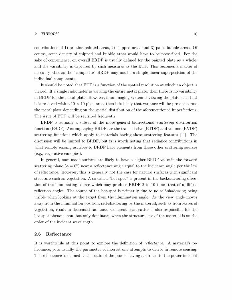
contributions of 1) pristine painted areas, 2) chipped areas and 3) paint bubble areas. Ofcourse, some density of chipped and bubble areas would have to be prescribed. For thesake of convenience, on overall BRDF is usually defined for the painted plate as a whole,and the variability is captured by such measures as the BTF. This becomes a matter ofnecessity also, as the “composite” BRDF may not be a simple linear superposition of theindividual components.

It should be noted that BTF is a function of the spatial resolution at which an object isviewed. If a single radiometer is viewing the entire metal plate, then there is no variabilityin BRDF for the metal plate. However, if an imaging system is viewing the plate such thatit is resolved with a 10 × 10 pixel area, then it is likely that variance will be present acrossthe metal plate depending on the spatial distribution of the aforementioned imperfections.The issue of BTF will be revisited frequently.

BRDF is actually a subset of the more general bidirectional scattering distributionfunction (BSDF). Accompanying BRDF are the transmissive (BTDF) and volume (BVDF)scattering functions which apply to materials having those scattering features [11]. Thediscussion will be limited to BRDF, but is is worth noting that radiance contributions inwhat remote sensing ascribes to BRDF have elements from these other scattering sources(e.g., vegetative canopies).

In general, man-made surfaces are likely to have a higher BRDF value in the forwardscattering plane (φ = 0) near a reflectance angle equal to the incidence angle per the lawof reflectance. However, this is generally not the case for natural surfaces with significantstructure such as vegetation. A so-called “hot spot” is present in the backscattering direc-tion of the illuminating source which may produce BRDF 2 to 10 times that of a diffusereflection angles. The source of the hot-spot is primarily due to no self-shadowing beingvisible when looking at the target from the illumination angle. As the view angle movesaway from the illumination position, self-shadowing by the material, such as from leaves ofvegetation, result in decreased radiance. Coherent backscatter is also responsible for thehot spot phenomenon, but only dominates when the structure size of the material is on theorder of the incident wavelength.

2.6 Reflectance

It is worthwhile at this point to explore the definition of reflectance. A material’s re-flectance, ρ, is usually the parameter of interest one attempts to derive in remote sensing.The reflectance is defined as the ratio of the power leaving a surface to the power incident

2 THEORY 17

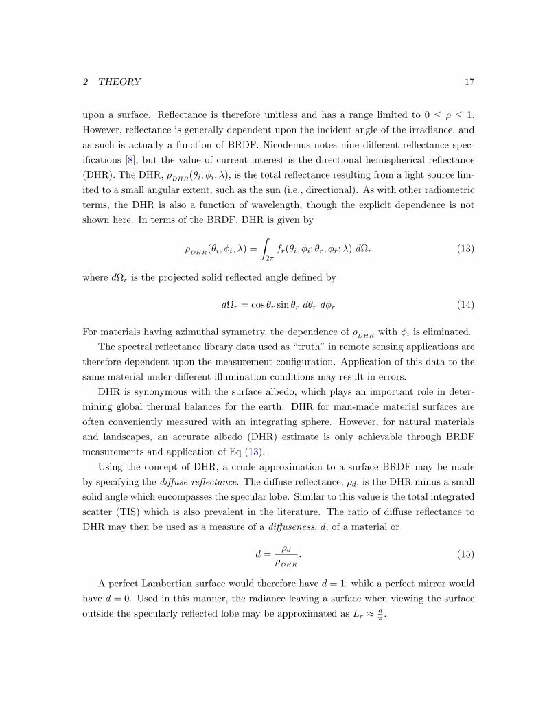
upon a surface. Reflectance is therefore unitless and has a range limited to 0 ≤ ρ ≤ 1.However, reflectance is generally dependent upon the incident angle of the irradiance, andas such is actually a function of BRDF. Nicodemus notes nine different reflectance spec-ifications [8], but the value of current interest is the directional hemispherical reflectance(DHR). The DHR, ρDHR(θi, φi, λ), is the total reflectance resulting from a light source lim-ited to a small angular extent, such as the sun (i.e., directional). As with other radiometricterms, the DHR is also a function of wavelength, though the explicit dependence is notshown here. In terms of the BRDF, DHR is given by

ρDHR(θi, φi, λ) =∫

2πfr(θi, φi; θr, φr;λ) dΩr (13)

where dΩr is the projected solid reflected angle defined by

dΩr = cos θr sin θr dθr dφr (14)

For materials having azimuthal symmetry, the dependence of ρDHR with φi is eliminated.The spectral reflectance library data used as “truth” in remote sensing applications are

therefore dependent upon the measurement configuration. Application of this data to thesame material under different illumination conditions may result in errors.

DHR is synonymous with the surface albedo, which plays an important role in deter-mining global thermal balances for the earth. DHR for man-made material surfaces areoften conveniently measured with an integrating sphere. However, for natural materialsand landscapes, an accurate albedo (DHR) estimate is only achievable through BRDFmeasurements and application of Eq (13).

Using the concept of DHR, a crude approximation to a surface BRDF may be madeby specifying the diffuse reflectance. The diffuse reflectance, ρd, is the DHR minus a smallsolid angle which encompasses the specular lobe. Similar to this value is the total integratedscatter (TIS) which is also prevalent in the literature. The ratio of diffuse reflectance toDHR may then be used as a measure of a diffuseness, d, of a material or

d =ρd

ρDHR

. (15)

A perfect Lambertian surface would therefore have d = 1, while a perfect mirror wouldhave d = 0. Used in this manner, the radiance leaving a surface when viewing the surfaceoutside the specularly reflected lobe may be approximated as Lr ≈ d

π .

2 THEORY 18

2.7 Polarimetric BRDF

Polarimetric BRDF is a more generalized case of the scalar BRDF. In addition to quan-tifying the magnitude of the directional scattering, the polarization of the scattering ischaracterized. In general, the change in polarized radiometric flux upon transmission orreflection from a medium is given by

Sr = M Si (16)

where M is a polarization transfer function called the Mueller matrix. The Mueller matrixis a 4 × 4 matrix which completely characterizes the polarized reflection or transmissionproperties of a medium for any incident Stokes vector, Si. Most often in remote sensing,interest will be limited to the reflection properties, or Mr.

Invoking the assumption that circular polarization is not present in a significant amountupon reflection from most surfaces [2, p. 486] reduces the Mueller matrix to a 3 × 3 matrixand the Stokes vector to a three element vector. With this reduction in dimensionality, Eq(16) may be explicitly written as S0r

S1r

S2r

=

m00 m01 m02

m10 m11 m12

m20 m21 m22

S0i

S1i

S2i

(17)

As described in Section 2.1, the radiometric quantities of Eq (10) become Stokes vectors.The generalized polarimetric BRDF is thus represented as

Mr(θi, φi; θr, φr;λ) =d~Lr(θr, φr)

d ~E(θi, φi)(18)

Mueller matrix notation is most often used to describe transmissive mediums (such asoptics) which results in unitless Mueller matrices. Also, the matrix is frequently normal-ized such that the m00 element is 1 and the multiplicative constant dropped—this notationreadily represents the medium’s polarization characteristics at the expense of the net trans-mission. When representing BRDF using Mueller matrices, the matrix has units of sr−1

as expected, and multiplicative constants should be maintained. In this manner the m00

element remains equivalent to the scalar BRDF value.A few representative Mueller matrices for ideal transmissive polarization filters are

provided in Eq (19), which will be referenced when discussing polarimetric BRDF mea-

2 THEORY 19

surements (§ 3.6).

M =12

1 1 01 1 00 0 0

M: =12

1 −1 0−1 1 00 0 0

(19a)

M =12

1 0 10 0 01 0 1

M; =12

1 0 −10 0 0−1 0 1

(19b)

M~ =

1 0 00 1 00 0 1

Mdep =

1 0 00 0 00 0 0

(19c)

The subscripts , :, , and ; represent the linear transmission orientation and are forhorizontal, vertical, +45 and -45 (or +135), respectively. A filter having no effect is theidentity matrix, shown as M~. A completely depolarizing filter is given by Mdep.

As with the scalar BRDF, energy conservation is maintained by recalling the relation-ship with DHR from Eq (13).

ρDHR(θi, φi) =∫

2πm00(θi, φi; θr, φr;λ) dΩr (20)

A good review of polarized BRDF representations is provided by Flynn [12].

3 MEASUREMENT 20

3 Measurement

The key elements of any optical scatter measurement are the sample material or object tobe measured, the illumination source and the detector. Most BRDF measurement devicesemploy one or more goniometric arms which provide angular positioning of the sourceand/or detector element. In some cases, the sample orientation may also be changed inorder to achieve the full hemispherical range of source and detector orientations.

Commercial BRDF measurement systems have been developed and are available fromat least two manufacturers. However, most measurement needs are satisfied with systemscustomized to the user’s unique application. It is for this reason, in part, that very fewBRDF databases exist. Measurements taken by a particular group often have inadequatematerial and experimental conditions described, and have tailored features which are noteasily adaptable to a new user’s interest.

Newer approaches in BRDF measurement often incorporate imaging techniques whichenable the the simultaneous sampling of multiple angles, greatly decreasing the requirednumber of measurements. Imaging systems also enable characterization of the bidirectionaltexture function (BTF). Other novel techniques have also been developed and will be brieflyexplored. The impetus for most of the newer measurement approaches are for improvedrendering in computer animation and simulation, in which there is a significant commercialmarket.

Outdoor BRDF measurements are common for remote sensing due to the large spatialscales of the materials involved, as well as the inability to bring representative materialsinto the lab, such as undisturbed live vegetation. Approaches toward outdoor BRDFmeasurements will be reviewed, as well as the means to handle some of the challengesoutdoor measurements present.

Finally, the measurements required to capture the most general form of BRDF, thepolarimetric BRDF will be reviewed. The foregoing measurement techniques may all beadapted to polarimetric measurements, with varying levels of complexity.

3.1 Commercial Devices

A small number of commercial devices are available for measuring directional reflectance.Surface Optics Corporation markets the SOC 200 Bidirectional Reflectometer, which is afull BRDF measurement device. The SOC 200 allows the use of laser sources, or a broadsource combined with a filter wheel system.3 Such a system may cost > $500 K [13] and is

3www.surfaceoptics.com/index.htm

3 MEASUREMENT 21

usually not warranted for most research needs.Surface Optics also offers other hand-held portable devices which function in the mid-

to far-infrared. Termed the “SOC 600,” it is advertised as a handheld imaging reflectometerand operates at 3–5 µm or 8–12 µm with angles of incidence up to 85. A pre-productionversion of the SOC 600 is described in [14] and was developed with funding in part fromthe Air Force Research Lab. The pre-production version has a measurement area of only 4mm2 and uses a microbolometer imaging array with an ellipsoidal mirror to sample multiplereflection angles using the 7.75 lb measurement head.

An alternate Surface Optics Corp. device, the SOC 250 was designed for portabilityand operation over the VNIR (400–1100 nm) or in the IR (3.0–12.0 µm) range [15]. Themeasurement head weighs ∼ 60 lbs and is accompanied by a power supply and laptopcomputer, which provides automated positioning of the source and detector. However, thesize of the device requires short detector and illumination standoff distances, as well as asmall measurement area.

Schmitt Industries, Inc., offers similar products including the CASI c© (Complete An-gle Scattering Instrument) which uses a laser source and has a high angular resolution.(0.001)4 A portable device, the µScan c© provides measurements using a laser diode andfixed angle of incidence.

The portable commercial devices are typically used in quality assurance applications todetermine if surfaces meet a required specification. They are often not suitable for materialgeometric and spectral BRDF characterization, in particular where larger sample sizes arerequired.

3.2 Conventional Laboratory Measurements

The most common and traditional means of measuring BRDF is to use an illuminationsource of small angular extent and a corresponding radiometer to measure the scatteredradiance. Several means of acquiring the necessary source and detector angular samplingare invoked by using a goniometer. For most systems, it is easiest to fix the source positionand vary the detector location to sample θr and φr. The incident angle, θi is sampledby moving the target sample, which is usually a relatively small, planar sample. In othercircumstances where the detector system may be large, such as a spectrometer, the detec-tor position is fixed and the source and the source and sample are moved to sample thehemisphere [16].

4www.schmitt-ind.com/products-services-measurement-systems-casi.shtml

3 MEASUREMENT 22

Illumination sources may either be lasers, or a broad-band source coupled with spectralfilters at the source or detector to enable spectral measurements. Often the data acquisitionprocess is automated, whereby the angular position of the detector and material is changedto cover the prescribed BRDF measurement sampling density. The number of required mea-surements is significant. For an isotropic material (no azimuth dependency) and samplingat 10 increments in both θi, θr and φ, the number of required measurements is exceeds1500 per spectral band (9 (0 ≤ θi ≤ +80)× 9 (0 ≤ θr ≤ +80)× 19 (0 ≤ φ ≤ +180)).If the material does not have azimuthal symmetry, an additional multiplier of 72 or morethan 100,000 measurement per spectral band is required! This simple calculation illustratesthe challenge in adequately measuring BRDF.

Lab measurements intended for remote sensing applications are particularly challenging.The heterogeneity or texture of most natural materials occurs at a spatial scale much largerthan the typical sample size which is used in the laboratory. For this reason, naturalmaterials are best measured over larger spatial scales and in their natural, undisturbedstates by outdoor measurement techniques (§ 3.4). However, BRDF measurements of man-made materials, which often constitute “targets” in spectral detection algorithms, maybe more accurately measured in the controlled lab environment. A review of BRDF labmeasurements with a remote sensing perspective is provided by Sandmeier [17].

3.3 Camera-based Measurements

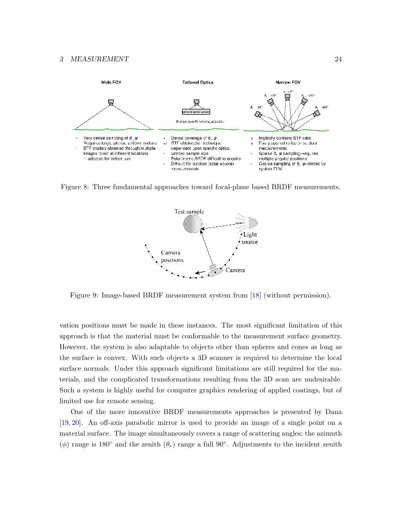
The use of focal planes to make BRDF measurements greatly increases the measurementefficiency. Rather than having a single detector, and hence a single bistatic angle foreach measurement, multiple reflection angles may be simultaneously acquired. Severalpermutations on this concept may be employed. BRDF measurement techniques usingfocal planes may be grouped into three basic approaches:

1. Wide field of view (FOV) sampling many reflecting angles

2. Tailored optics systems to image the material (many variants)

3. Narrow FOV used similar to a single element detector

The wide FOV systems rely upon a large uniform material area for making measure-ments. Discrete scattering angles are obtained from each pixel of the imaging system,which enables an efficient, dense sampling of scattering angles. Of course, spatial inhomo-geneities in the material erroneously manifest themselves as a BRDF change so caution

3 MEASUREMENT 23

must be used. Several outdoor systems make use of this measurement approach and willbe addressed separately in § 3.4.

The second basic imaging configuration, tailored optics systems, encompasses a numberof measurement concepts and are among the most creative. The overall approach is to re-image the material surface in a manner which enables efficient changes to the system, suchas the incident angle of illumination and multiple viewing geometries. Two such approachesare included here, one which images an infinitesimal surface point, and another employing akaleidoscope which provides multiple discrete scattering angles while resolving the surface.The most significant disadvantages of these systems are the limitations imposed upon theilluminating source and the sample size—outdoor measurements using the sun would bedifficult. Also, since these systems use reflective optics having multiple reflections or varyingreflectance angles, measuring the polarimetric BRDF is problematic due to the polarizationdependency of the system.

Finally, a narrow FOV imaging system may be used, analogous in the manner of asingle element detector. Implicit in this measurement technique is the BTF from theimage data. However, as with a single detector, many measurements or images must beacquired to cover the scattering hemisphere. Therefore, this technique must heavily relyupon BRDF models to inter/extrapolate the data. This technique is adaptable to boththe lab and field. For field use, calibration and stray light mitigation are readily employed.Systems using this approach have not been noted in the literature, likely due to the singlescattering angle sampling. However, it is this technique which the author recommendsfor high spatial-resolution remote sensing, as will be seen in Section 6. These three basicimaging approaches to BRDF measurement, along with their relative merits are illustratedin Figure 8.

The following approaches are those of the “tailored optics systems.” As previouslymentioned, wide FOV systems will be addressed in § 3.4 and the new narrow FOV systemsin § 6.

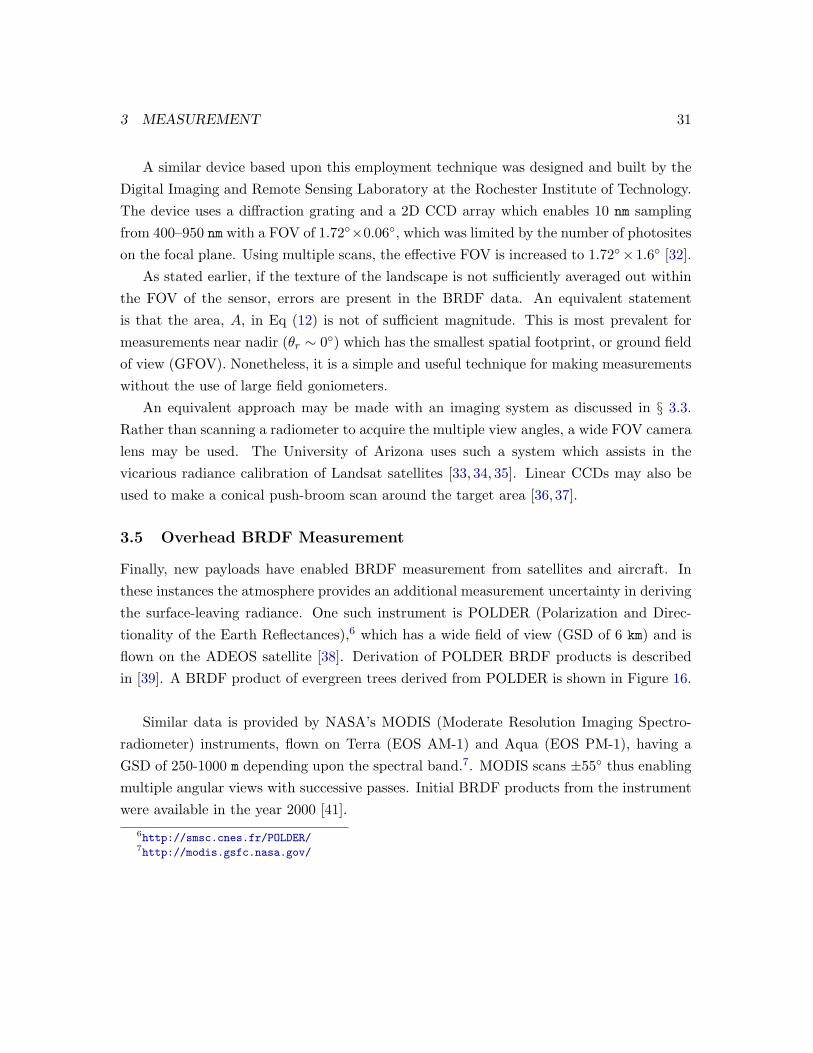
Marschner reports a system which images an object of known shape, such as a sphereor a cone, covered with a desired material to be measured [18]. The shape of the objectinherently provides the multiple viewing geometries rather than using optics. Viewing theobject while having a single illumination source enables the direct measurement of a largenumber of incident and scattering angles with a single image. Scanning either the sourceor the camera in a single plane enables sampling the full hemisphere of source and detectorangular positions. A diagram illustrating this approach is shown in Figure 9. Appropriatecoordinate transformations relating the local surface normal to the illumination and obser-

3 MEASUREMENT 24

Figure 8: Three fundamental approaches toward focal-plane based BRDF measurements.

Figure 9: Image-based BRDF measurement system from [18] (without permission).

vation positions must be made in these instances. The most significant limitation of thisapproach is that the material must be conformable to the measurement surface geometry.However, the system is also adaptable to objects other than spheres and cones as long asthe surface is convex. With such objects a 3D scanner is required to determine the localsurface normals. Under this approach significant limitations are still required for the ma-terials, and the complicated transformations resulting from the 3D scan are undesirable.Such a system is highly useful for computer graphics rendering of applied coatings, but oflimited use for remote sensing.

One of the more innovative BRDF measurements approaches is presented by Dana[19, 20]. An off-axis parabolic mirror is used to provide an image of a single point on amaterial surface. The image simultaneously covers a range of scattering angles; the azimuth(φ) range is 180 and the zenith (θr) range a full 90. Adjustments to the incident zenith

3 MEASUREMENT 25

Figure 10: A novel BRDF measurement approach using an imaging system and a parabolicmirror to simultaneously acquire multiple scatter angles. Used without permission from [20]

.

angle (θi) are possible with a simple planar translation of the light source aperture. In asimilar manner, multiple image points on the material surface are obtained by translatingthe parabolic mirror above the surface. The multiple image points enable texture (BTF)measurements or the spatial “micro-scale” variation of BRDF (§ 2.5). A schematic overviewof the Dana measurement technique is provided in Figure 10. A similar approach is alsoreported by Apel [21].

Another unique approach has been implemented by Han [22] which employs imagingthrough a kaleidoscope to enable the simultaneous measurement of the BRDF and BTF.A tapered kaleidoscope having front-surface mirrors is used to image a material, whichcreates a virtual sphere consisting of multiple, tapered facets corresponding to differentviewing zenith angles of the object. The effect is equivalent to having multiple cameraangles imaging the same surface area. A digital projector provides the light source and theincident illumination angles are controlled by selectively turning on groups of pixels in thedigital projector. A beam splitter is used to merge the optical paths of the illuminationsource and the camera. The taper angle of the kaleidoscope controls the number of facetsviewed, or equivalently the number of scattering angles sampled. A smaller taper angleincreases the number of facets, but has the disadvantage of lower spatial sampling whenimaged by the camera. The converse is true of a larger taper angle. This concept isillustrated in Figure 11.

3 MEASUREMENT 26

Figure 11: BRDF and BTF measurement using a kaleidoscope. The setup (left) uses acommercial digital projector and digital camera as the light source and detector. An imageof a penny through the system with a narrow-taper kaleidoscope provides a total of 79whole facets, which may be used to generate 792 unique illumination viewing geometries.Used without permission from [22].

3.4 Field Measurements

Portable BRDF devices suitable for outdoor measurements are attractive for a numberof reasons. The use of portable devices arises out of necessity when measurements mustbe made which are extremely difficult, if not impossible to replicate in the lab. Naturalmaterials may be heterogeneous over spatial extents significantly larger than what may bemeasured in the lab. Vegetation is a classic example of one such material, whether it isgrass or a leaf canopy. Direct measurement of materials in their natural state and at largerspatial scales eliminates the requirement to scale-up individual material BRDFs which areoften interactive, such as leaf transmittance and multiple leaf adjacency effects. Havingthe use of the sun as the source is advantageous as well. A good review of BRDF fieldmeasurements in the VNIR is given by Walthall [23].

An obvious challenge to outdoor measurements is cooperative weather and stray light.A nice day may eventually be found (even in Rochester, NY), but the downwelled radianceoutside the solar disk is always an error source in the measurements. In addition, themagnitude and distribution of this error source changes depending on local atmosphericconditions, such as extent of cloud cover. This error source obviously has a spectral de-pendence, as the blue sky testifies. A good discussion of outdoor measurement errors and

3 MEASUREMENT 27

minimization techniques is provided by Sandmeier [24] with some quantitative assessmentsprovided by [25, 26]. Techniques for minimizing these errors will be discussed concurrentwith the recommended BRDF measurement approach in § 6.1.4. Finally, the source zenithposition is not easily adjustable (unless you’re Clark Kent).

In most circumstances, outdoor measurements are made over a sample spatial extentmuch greater than that made with lab measurements. The basic criteria regarding whatconstitutes a sufficient area for measurement still applies (as discussed in Section 2). Highspatial frequency inhomogeneities in the material must be adequately averaged out over themeasured sample area. For example, if the material of interest is grass, then the measuredarea must encompass many individual blades of grass which integrates out the individualblade detail. An indication of adequate sample size is when the resulting BRDF valueis relatively insensitive to changes in the sample area in the field of view (FOV) of theinstrument, or equivalently as the variance in the BTF approaches zero for increasing ∆x

and ∆y.A highly relevant challenge, though outside the scope of this treatment, is generating

a sufficiently accurate and meaningful descriptive characterization of the material, whichis critical for natural materials. It is by these descriptive labels that the acquired datawill be selected and used in subsequent analysis, synthetic image generation, etc. A simpledescriptor such as “Paint XYZ on Aluminum” is not sufficient when ascribing BRDF toinhomogeneous targets.5 It is suggested that a robust meta-data set always accompany suchmeasurements. This meta-data should include photographs of various viewing geometriesof the sample, as well as detailed verbal descriptors.

A review is now provided of some field devices reported in the literature. Two fun-damental designs may be employed. A traditional “lab-like” system where the sensor ismoved around a hemisphere above the target, or one in which the sensor does not translate,but acquires different view angles from the fixed position. With the latter type system, thetarget area must be sufficiently uniform such that views of each area are each representativeof one another.

3.4.1 Mobile Sensor Designs

The most direct approach toward field BRDF measurements is to emulate a laboratorysetup by using a goniometer. With the illumination source (the sun) and target orientation

5Actually, adequately describing “simple” materials is very challenging also. Added to the description of“Paint XYZ on Aluminum” should also be information such as application method, surface condition andpaint thickness—and again a picture doesn’t hurt.

3 MEASUREMENT 28

Figure 12: An example of field goniometers for BRDF measurements. FIGOS is shown onthe left and the SFG system in the middle and right. From Sandmeier [24] (left and right)and [?] (middle) without permission.

on the ground fixed, the goniometer serves to move the detector to sampling positionsthroughout the hemisphere.

One such example of a system is FIGOS (field goniometer system) built by the RemoteSensing Lab of the University of Zurich [27, 28]. The system consists of a “zenith” arcof 2 m radius which rests on a circular frame of 4 m diameter–the azimuthal arc (Figure12). The sensor is a spectroradiometer providing coverage from 300–2450 nm with spectralresolution of 1.5 nm in the VIS and 8.4 nm in the SWIR providing a total of 704 bands. ThePC-controlled spectroradiometer, with a FOV of 2, is driven along the zenith arc by aDC motor to enable sampling θr. The entire zenith arc assembly is rotated on the azimutharc, providing φr sampling. The entire system weighs some 500 lbs and may be set upby a team of two in ∼ 90 min. Measurements are made at a resolution of ∆θr = 15 witha range of ±75 and ∆φr = 30. The 11 measurements made in each azimuth positionrequire 3 min for a total acquisition time of 18 min for all 66 hemispherical measurements.The mechanical structure cost ∼ $125, 000 (1994 USD) [28].

A nearly identical goniometer, the Sandmeier Field Goniometer (SFG) was constructedby NASA Ames based upon the FIGOS design. However, this field goniometer is fullyautomated and the acquisition time for the same angular sampling scheme as FIGOS(∆θr = 15,∆φr = 30) is completed in less than 10 min [24]. Figure 12 pictures theSFG and FIGOS systems.

Another goniometer advertised as having outdoor measurement capability was con-structed by ONERA in France. However, this system is much more massive with a weightapproaching 2000 lbs, but with individual components disassembled to ∼125 lbs. Thesystem provides spectral coverage from 400–1000 nm with a ∆λ of 3 nm. The target area isimaged with a bundle of 59 fiber optics and a fore optic. The fiber optics mixes the incident

3 MEASUREMENT 29

Figure 13: Goniometer for BRDF laboratory measurements [30].

polarization of the scattered radiance, thus eliminating the polarization dependency of thediffraction grating in the spectrometer [29,30]. This also enables polarimetric BRDF mea-surements using the device, to be addressed in § 3.6. The instrument is shown in Figure13.

The previous goniometer systems provide high angular precision and rapid samplingof the scattering hemisphere. They are suitable for highly accurate characterization offield materials. However, both systems require significant support for transport and setup,which is exacerbated by having to time the weather conditions for suitable measurementperiods. A much more simple measurement technique is often warranted which still providesmeaningful BRDF data. Representing this opposite extreme are simple measurements madewith a radiometer attached to a hand-held boom. The angular position of such a devicemay be estimated based on trigonometry of the height and distance from the measuredarea. Measurements of a only a few geometric positions provides an understanding of theBRDF anisotropy, or departure from a Lambertian surface. A simple boom system is shownin Figure 14.

3.4.2 Immobile Sensor Designs

An alternative approach to a sensor being repositioned around the hemisphere is a fixedsensor which changes the view angle over a large homogeneous measurement area. One suchBRDF measurement device is PARABOLA (Portable Apparatus for Rapid Acquisition ofBidirectional Observations of Land and Atmosphere), which has been used in various formsby NASA-Goddard since the mid-1980s [31]. Such a sensor is often mounted high on a mastor a lift in order for the FOV to average out spatial inhomogeneities in the landscape (Figure15).

3 MEASUREMENT 30

Figure 14: A simple hand-held boom BRDF measurement. From NASA (http://modarch.gsfc.nasa.gov/MODIS/LAND/VAL/prove/grass/prove.html) without permission.

Figure 15: The Parabola III system showing the sensor, and the sensor mounted on a boomfor field measurements. From NASA (http://modarch.gsfc.nasa.gov/MODIS/LAND/VAL/prove/grass/prove.html) without permission.

3 MEASUREMENT 31

A similar device based upon this employment technique was designed and built by theDigital Imaging and Remote Sensing Laboratory at the Rochester Institute of Technology.The device uses a diffraction grating and a 2D CCD array which enables 10 nm samplingfrom 400–950 nm with a FOV of 1.72×0.06, which was limited by the number of photositeson the focal plane. Using multiple scans, the effective FOV is increased to 1.72×1.6 [32].

As stated earlier, if the texture of the landscape is not sufficiently averaged out withinthe FOV of the sensor, errors are present in the BRDF data. An equivalent statementis that the area, A, in Eq (12) is not of sufficient magnitude. This is most prevalent formeasurements near nadir (θr ∼ 0) which has the smallest spatial footprint, or ground fieldof view (GFOV). Nonetheless, it is a simple and useful technique for making measurementswithout the use of large field goniometers.

An equivalent approach may be made with an imaging system as discussed in § 3.3.Rather than scanning a radiometer to acquire the multiple view angles, a wide FOV cameralens may be used. The University of Arizona uses such a system which assists in thevicarious radiance calibration of Landsat satellites [33, 34, 35]. Linear CCDs may also beused to make a conical push-broom scan around the target area [36,37].

3.5 Overhead BRDF Measurement

Finally, new payloads have enabled BRDF measurement from satellites and aircraft. Inthese instances the atmosphere provides an additional measurement uncertainty in derivingthe surface-leaving radiance. One such instrument is POLDER (Polarization and Direc-tionality of the Earth Reflectances),6 which has a wide field of view (GSD of 6 km) and isflown on the ADEOS satellite [38]. Derivation of POLDER BRDF products is describedin [39]. A BRDF product of evergreen trees derived from POLDER is shown in Figure 16.

Similar data is provided by NASA’s MODIS (Moderate Resolution Imaging Spectro-radiometer) instruments, flown on Terra (EOS AM-1) and Aqua (EOS PM-1), having aGSD of 250-1000 m depending upon the spectral band.7. MODIS scans ±55 thus enablingmultiple angular views with successive passes. Initial BRDF products from the instrumentwere available in the year 2000 [41].

6http://smsc.cnes.fr/POLDER/7http://modis.gsfc.nasa.gov/

3 MEASUREMENT 32

Figure 16: Space-based BRDF measurement of “broadleaf evergreen trees” by POLDER.From [40] without permission.

3.6 Polarimetric BRDF Measurement

As noted in § 2.7, one quantifies the reflective Mueller matrix, Mr, in making polarimetricBRDF measurements [Eq (18)]. In polarimetric BRDF measurements, the scattered orreflected Stokes radiance vector, ~L, must be quantified such that

~L(θr, φ) = Mr(θi, φ, θr) ~E(θi) (21)

However, without the use of any polarization filtering, the detector only measures themagnitude of the irradiance and radiance as in the case of the scalar BRDF or

L0(θr, φ) = m00(θi, φ, θr)E0(θi) (22)

where the “0” subscript denotes the first element of the Stokes vector, which is the totalflux and m00 is the upper left element of the Mueller matrix equivalent to the scalar BRDF.

Clearly, additional measurements are needed to characterize the other 15 elements ofthe Mueller matrix. When considering linear polarization, this requirement is reduced todetermining the remaining 8 elements of the 3×3 Muller matrix. These additional elementsof the array may be determined by linear combinations of incident irradiance polarizationstates, ~E, and received polarization radiance states, ~L.

The most generalized means of acquiring the matrix elements is through presentingmultiple incident polarization states, and measuring the output for each incident state,thus building a system of linear equations. The polarization filters which create incidentpolarization states are termed generators while those which filter the output are calledanalyzers. The presentation of i incident polarization states onto the sample and their

3 MEASUREMENT 33

polarized radiance measurements may be represented as

Mr

[~E1

~E2 · · · ~Ei−1~Ei

]=[

~L1~L2 · · · ~Li−1

~Li

](23)

where[

~E1~E2 · · · ~Ei−1

~Ei

]is a 4× i matrix consisting of irradiance column Stokes vectors

and[

~L1~L2 · · · ~Li−1

~Li

]is the equivalent radiance representation. Rewriting these terms

as matrix quantities E and L, the new expression is

MrE = L (24)

where it is seen thatMr = L E−1 (25)

However, inversion of E is only possible when it is a nonsingular square matrix. For thegeneral case where i > 4, the pseudoinverse of E is sought, E#, which provides a leastsquares estimate in the presence of random noise. The pseudoinverse is given by

E# =(ETE

)−1ET (26)

where T is the transpose of the matrix. The Mueller matrix is therefore solved by

Mr = L E# (27)

In this manner the full Mueller matrix may be determined for each permutation of θi, θr,φ and λ as one would measure the scalar BRDF.

For practical measurement considerations, one would like an efficient set of input andoutput polarization states to minimize the number of measurements. The equation describ-ing this measurement setup is given as

~L = MA Mr MG~E (28)

where MG is the generator filter over the source and MA is the analyzer filter over thedetector. Note that the generator and analyzer Mueller matrices have no units, but thereflectance Mueller matrix Mr has BRDF units, sr−1 (see also § 2.7).

Referencing the polarization filters provided by Eq (19), a simple example is constructed

3 MEASUREMENT 34

for generator and analyzer linear horizontal filters. The equation is given by

~L = M Mr M ~E (29)

or explicitly as L0

L1

L2

=12

1 1 01 1 00 0 0

m00 m01 m02

m10 m11 m12

m20 m21 m22

12

1 1 01 1 00 0 0

E0

E1

E2

(30)

which reduces to L0

L1

L2

=14

(m00 + m01 + m10 + m11) (E0 + E1)(m00 + m01 + m10 + m11) (E0 + E1)

0

(31)

However, it is only the L0 Stokes component that the detector will be measuring. If theoriginal source is highly randomly polarized, then E1 E0 and the measurement yields

L =(m00 + m01 + m10 + m11) E0

4(32)

In a similar manner, other permutations of generator and analyzer polarization statesproduce additional linear combinations of the Mueller matrix elements. A summary of suchcombinations is provided by Bicket [42]. To quantify the 3× 3 subset of Mr which relatesto linear polarization, a total of 9 measurement permutations is required which include thethree generator and analyzer states of horizontal, +45 and no (or random) polarization.These states are represented symbolically as , and ~, respectively. Using this symbolicrepresentation, Eq (32) may be recast as

=L

E0=

m00 + m01 + m10 + m11

4(33)

where the first “” represents the generator state, and the second “” is the polarization

3 MEASUREMENT 35

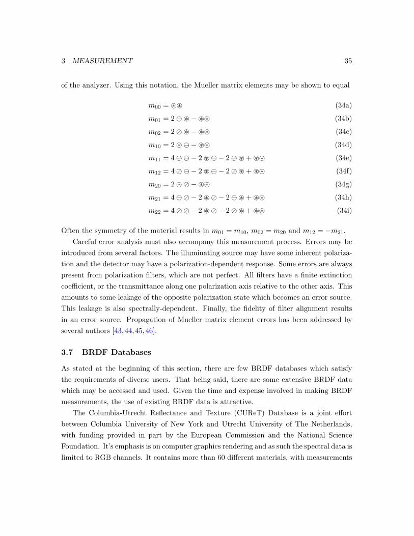
of the analyzer. Using this notation, the Mueller matrix elements may be shown to equal

m00 = ~~ (34a)

m01 = 2~−~~ (34b)

m02 = 2~−~~ (34c)

m10 = 2 ~−~~ (34d)

m11 = 4− 2 ~− 2~ + ~~ (34e)

m12 = 4− 2 ~− 2~ + ~~ (34f)

m20 = 2 ~−~~ (34g)

m21 = 4− 2 ~− 2~ + ~~ (34h)

m22 = 4− 2 ~− 2~ + ~~ (34i)

Often the symmetry of the material results in m01 = m10, m02 = m20 and m12 = −m21.Careful error analysis must also accompany this measurement process. Errors may be

introduced from several factors. The illuminating source may have some inherent polariza-tion and the detector may have a polarization-dependent response. Some errors are alwayspresent from polarization filters, which are not perfect. All filters have a finite extinctioncoefficient, or the transmittance along one polarization axis relative to the other axis. Thisamounts to some leakage of the opposite polarization state which becomes an error source.This leakage is also spectrally-dependent. Finally, the fidelity of filter alignment resultsin an error source. Propagation of Mueller matrix element errors has been addressed byseveral authors [43,44,45,46].

3.7 BRDF Databases

As stated at the beginning of this section, there are few BRDF databases which satisfythe requirements of diverse users. That being said, there are some extensive BRDF datawhich may be accessed and used. Given the time and expense involved in making BRDFmeasurements, the use of existing BRDF data is attractive.

The Columbia-Utrecht Reflectance and Texture (CUReT) Database is a joint effortbetween Columbia University of New York and Utrecht University of The Netherlands,with funding provided in part by the European Commission and the National ScienceFoundation. It’s emphasis is on computer graphics rendering and as such the spectral data islimited to RGB channels. It contains more than 60 different materials, with measurements

3 MEASUREMENT 36

for each consisting of more than 200 incident and scattering angle combinations. Detailson the database are in [9] and the database is accessible via the internet.8 Data files fora material are typically 100s of MB and fits are made to the data using the Oren-NayarBRDF model [47].

Cornell University’s computer graphics program maintains a similar database, also in-ternet accessible.9 The database primarily contains paint samples which are measuredwith high spectral (≤ 10 nm) and geometric resolution, but is limited to visible (VIS)wavelengths.

The Nonconventional Exploitation Factors (NEF) BRDF database contains BRDF mea-surements of more than 400 materials which are fit to a modified Maxwell-Beard BRDFmodel [48]. The measurement protocol used in acquiring the data is that recommendedby Maxwell [49]. Laser sources from the UV to LWIR are used to obtain the scattering inthe plane of incidence as well as the cross scattering (φr = ±90). Spectral interpolationis accomplished by a high spectral resolution DHR measurement, where it is assumed thatthe spectral BRDF change with orientation is a slowly varying function [48]. Materials cov-ered in the NEF are grouped into twelve general categories which include asphalt, brick,camouflage, composite, concrete, fabric, water, metal, paint, rubber, soil and wood. Thedatabase has been employed in rendering computer graphics [6, 50] as part of a project bythe National Institute of Standards and Technology.10

Surface Optics Corporation, discussed previously in Section 3.1, maintains an opticalproperties database which primarily includes DHR measurements. The data may be pur-chased in whole or in part and includes some 180 materials grouped into categories whichinclude construction materials, fabrics, paints, rocks, soils and vegetation. Only a subsetof the materials includes BRDF data which was acquired over three broad bands: VIS,MWIR and LWIR.11

Finally, numerous spacecraft and optical component BRDF data are consolidated inSOLEXISTM, a database created and maintained by Stellar Optics Research InternationalCorporation (SORIC).12 The database appears to primarily contain in-plane scatteringmeasurements, and the emphasis is on stray light for thermo-optical components. Datawas collected from a large number of public and private sources [51].

8http://www1.cs.columbia.edu/CAVE/curet/9http://www.graphics.cornell.edu/online/measurements/reflectance/index.html

10http://math.nist.gov/∼FHunt/appearance/nefdsimages.html11http://www.surfaceoptics.com/brochures/SOC Measured Data Doc.pdf12http://www.soric.com

4 MODELS 37

4 Models

As has been seen, an infinite number of measurements is required to fully quantify BRDF.The difficulty in making and managing BRDF datasets necessitates the use of BRDFmodels. BRDF models are motivated from several factors:

1. Compactness: Individual material data sets with high angular and spectral samplingmay easily exceed 100 MB, and if a scene is considered which contains hundreds ofmaterials, the volume of data is unmanageable. A BRDF model provides a concisemeans of storing the data.

2. Interpolation: Often only sparse hemispherical sampling has been measured for sam-ples, in which case a means of inter- or extrapolating the measured values is required.

3. Prediction: No BRDF measurements have been made for a material, but the physicalattributes of the material are known which enable prediction of the BRDF.

4. Information Extraction: In fields such as remote sensing and semiconductor process-ing, BRDF models may be linked to physical attributes such as leaf area index whichprovide target information.

Virtually all BRDF models satisfy the need for compactness, and most provide somemeans of interpolation. Models providing prediction without any measured data are first-principles, physics based and are attractive since empirical data is not needed. Manymodels are prediction models which use a modest amount of empirical data, to which someconstants or parameters are fit. Finally, models which provide information extraction areusually tailored to a specific target classes of interest, such as erectophile vegetation orconifer forests.

There are seemingly an infinite number of BRDF models, derived from many re-searcher’s dissatisfaction with attempting to apply existing models to their specific interestarea. Surprisingly (at least to a physical scientist), the computer graphics communityhas made substantial contributions to the field as processing power has enabled three-dimensional rendering of objects. Of course, there is a significant commercial market forthese applications which continues to drive development.

The BRDF models covered in this section are limited to those for homogeneous mate-rials. That is, models which describe a highly uniform surface with minimal texture suchas common with man made materials. Thus they are suitable for describing surfaces whichare often “target materials” in spectral algorithms. Heterogeneous material BRDF models,

4 MODELS 38

such as those commonly used in remote sensing for complex vegetation canopies are verydistinct from the homogeneous material models. These models may be used to describe“background materials” in spectral algorithms. It is rare to find a remote sensing publica-tion which references homogeneous BRDF models common to the optics and radiometrycommunity. Discussion of remote sensing BRDF models is postponed until § 5.4.

BRDF models may be classified in a number of ways. One classification is based uponthe treatment of the optics. Geometric optics models are in general more approachable, butthe underlying ray model assumptions break down as surface roughness dimensions decreaseand become proportional to or less than the wavelength. Models based on physical opticsprovide a much more thorough treatment through field equations, but result in complicatedexpressions.

BRDF models may also be classified as physical or empirical. Physical models relyupon first-principle physics of electromagnetic energy and material interactions, and requireinputs such as surface roughness parameters and the complex index of refraction. Empiricalmodels rely solely upon measured BRDF values, while semi-empirical models incorporatesome measured data, but may have significant elements of physics-based principles. Thesesemi-empirical models are perhaps the most common and versatile.

Many BRDF models divide a surface into microfacets, for which the distribution of theindividual microfacet normals drives the specular and diffuse scattering contributions, aspreviously discussed when considering optical scatter and illustrated in Figure 4. Thesemodels require the use of spherical trigonometry which relates the local microfacet coordi-nate system to the material surface coordinate system.

Recently, polarized BRDF (pBRDF) models have been developed which predict thepolarized radiance as discussed in § 2.7. Such models are a prerequisite to the quantitativeanalysis of polarimetric images in remote sensing. The polarized models are usually enabledby using the Mueller matrix representation of the microfacet reflections. Two of the pBRDFmodels reported in the literature have been enabled by adapting an existing BRDF modelto include polarization effects.

Finally, the question of required accuracy must be addressed. A systems engineeringapproach to this question is appropriate, as the required accuracy of any BRDF modeldepends upon the specific application, as well as the magnitudes of other radiometricerrors present in the remote sensing imaging chain. It is suggested that the accuracy ofmany of the models discussed below is more than sufficient in remote sensing applications.Consider a spectral target detection algorithm. An assumption must be made regardingthe orientation of the target relative to the local horizon. The most obvious assumption is

4 MODELS 39

that the target is on level ground. However, deviations of ±20 are not difficult to consider(e.g., the slope of the front of a vehicle, a vehicle on a modest hill, etc.). More discussionon target orientation will be provided in § 5.

4.1 Early BRDF Models

Though often not considered a BRDF model, the Lambertian assumption ascribes a con-stant BRDF for all incident and reflecting geometries [1]. It is simply

fr =ρ

π(35)

where ρ is the reflectance. This is traditional treatment of reflectance in remote sensing.One of the earliest variable BRDF models was proposed by Minnaert in 1941 to account

for darkening near the lunar limb [52]. It is represented by

fr =ρ (cos θr cos θi)

k−1

π(36)

where k is the “limb darkening” parameter. Note for k = 1, it is equivalent to Lambert’sBRDF.

Astronomical observation was responsible for significant BRDF work. In particular,physical explanations of the “hot spot” effect for planetary bodies was sought. Analysiswas also performed in attempts to better understand the surface of the moon for prepa-ration for the lunar landings. Toward this end, Hapke developed what is known as theHapke/Lommel-Seeliger BRDF model which accounted for opposition effects [53]. Thiswork concluded that the lunar surface was composed of fine, compacted dust, and themodel would later form the basis of the popular semi-empirical model by Maxwell-Beard.

4.2 Empirical Models

The most straightforward means of producing BRDF data for all incident and scatteringangles is simply by interpolation of empirical data, which may be viewed by some ascircumventing a BRDF model altogether. Here, no physical basis of the scattering isconsidered, and the only inputs are the empirical measurements. This approach is attractivedue to the simplicity.

Such an approach has been used by the University of Zurich’s Remote Sensing Lab-oratories for outdoor measurements using the BRDF measurement system described in

4 MODELS 40

Figure 17: BRDF data for grass at 600 nm interpolated using spherical Delaunay triangu-lation with ∼70 measurements (left) and ∼400 measurements (right). Data acquired withthe FIGOS system (see § 3.4.1). From [54] without permission.

Section 3.4 [27, 28]. An example of fitting BRDF data for lawn grass is shown in Fig-ure 17 at 600 nm for an incident solar angle of θi = 35. Here, interpolation is accom-plished by spherical Delaunay triangulation, with the left figure having a sampling of∆θr = 15;∆φ = 30 (∼70 measurements) and the right figure having a ∼sixfold in-crease in sampling at ∆θr = 5;∆φ = 15 (∼400 measurements). While there is a markedchange in the peak magnitude around the “hot spot” or retroreflection position, the otherangular positions in the coarser sampling appear to have only minor variations.

The data shown in Figure 17 was made using an IDL software package from the Univer-sity of Zurich called GONIO.13 A copy of GONIO has been acquired, which also includesan ENVI interface. GONIO handles multispectral BRDF data and provides interpolationof sparse data sets via IDL’s Triangulate function. Further exploration of this package iswarranted to investigate the utility it may have for the DIRS group.

Interpolation of measured data is highly accurate so long as measurements are madewith reasonable sampling densities. However, as the geometric sampling density increases,so does the accuracy, but at the expense of massive data storage requirements (see §3.2). Measured BRDF values may be decomposed into appropriate basis functions havingspherical or circular symmetry, greatly reducing the storage requirements for measureddata sets.

Spherical harmonics may be used as a basis set to represent an arbitrary BRDF, analo-gous to the manner in which a Fourier series may be used to represent a function. However,

13http://www.geo.unizh.ch/rsl/research/SpectroLab/goniometry/index.shtml

4 MODELS 41

a significant number of coefficients may be required for accurate representation, and ring-ing may be present from series truncation [55]. As an alternative to spherical harmonics,the hemisphere may be projected onto a single plane and Zernike polynomials used [56].In a similar manner, spherical wavelets may also be used [57]. Other ideas for efficientrepresentation include transforming BRDF variables by taking advantage of symmetries toreduce the number of basis function coefficients required [58].

4.3 Semi-empirical Models

4.3.1 Torrance-Sparrow

In 1967 Torrance and Sparrow presented one of the first BRDF models to capture suchphenomena as the off-specular peak, as well as providing good predictions as θr → 90 [59].The Torrance-Sparrow (T-S) model is developed on the basis of geometrical optics, and assuch it requires the RMS surface roughness, σm, to be comparable to or greater than thewavelength considered (σm/λ & 1.0). As with many BRDF models, the contributions of in-dividual microfacet reflections to the overall material BRDF is considered. Each microfacetof area Af is treated as a specular surface, for which the surface normals are distributedaccording to a gaussian probability distribution, P (α). The diffuse BRDF component ofthe BRDF arises from multiple microfacet reflections or internal scattering. Therefore, thereflected radiance, Lr may be expressed as the sum of the specular and diffuse components

Lr = Lr,s + Lr,d (37)

with the diffuse component given by

Lr,d = aLi cos θi (38)

where a is a constant.The specular reflection is obtained by considering the Fresnel reflection, F , off each mi-

crofacet according to Eqs (6 & 8). The significant advancement made by the T-S model wasthe introduction of a geometric attenuation factor, G, which enables masking and shadow-ing. Masking is the blockage of specular reflections by adjacent microfacets while shadowingis the blockage of the illumination source onto a microfacet by adjacent microfacets. The

4 MODELS 42

resulting BRDF from the T-S model is given as

fr =F (θ

′i, n) Af G(θi,p, θr,p) P (α)

4 cos θi cos θr+

a

dωi(39)

where the second term is the diffuse component and the primed coordinate system is rel-evant to the microfacet normal. The θX,p coordinates result from projections of θi and θr

onto the plane determined by the facet and surface normals. n is the complex index ofrefraction given by n− ik.

So what parameters are required for producing T-S BRDF predictions? To obtain theFresnel reflectance, n is required. A roughness parameter, c, which relates the distributionof facet slopes relevant to the normal plane is required. Note that c is manifested inP (α) which is proportional to exp(−c2α2). T-S used a value of 0.05 which was justifiedbased on fitting the data to experimentally-determined BRDF. While T-S makes use offirst principles to model the BRDF, it nonetheless requires a parameter which they fit toexperimental data.

4.3.2 Maxwell-Beard

The development of the Maxwell-Beard (M-B) BRDF model was originally motivated foruse on painted surfaces [49]. The model development emphasizes BRDF prediction fromIR laser sources (1–4 µm) with varying polarization states. As with the Torrance-Sparrowmodel, separate diffuse and specular contributions to the BRDF are considered, whichMaxwell and Beard term surface and volume contributions.

With the surface model, only single reflections from the microfacet surface are consid-ered. The distribution of the microfacets are obtained through a monostatic scan in whichthe detector and illumination source are co-located, or as close to the same position with-out subtending each other. The surface normals of each microfacet are defined as beingoriented in the

(θN , φN

)direction. The measured signal of the monostatic scan may then

be related to the density of microfacets which fall within the detector solid angle, giving adensity of Ξ(θN , φN ) which has units of sr−1. Reflection from the microfacets is given bythe Fresnel reflectance, Eq (9).

In terms of these experimentally measured parameters, the surface model componentof the BRDF may be expressed as

frsurf(θi, φi; θr, φr) =RF (β)RF (0)

fr(θN ) cos2 θN

cos θi cos θr(40)

4 MODELS 43

where RF is the Fresnel reflectance, expressed in terms of half the angle between the sourceand receiver, where 2β is the bistatic angle or angle between the source and receiver. fr(θN )is the BRDF from the monostatic scan through the zenith position (i.e., −90 ≤ θi = θr ≤90). It is given by

fr(θN ) =RF (0)Ξ(θN , φN )

4 cos θi cos θr(41)

from which the microfacet density function is obtained.All information needed for Eq (40) is experimentally obtained. However, the Fresnel

reflectance requires the complex index of refraction, n, of the material. M-B assumedthe surfaces were dielectrics, a reasonable assumption for the paint samples they weremodelling, which makes k ≈ 0 or n = n. A value of n in their study was estimated asn = 1.65 and was based upon experience with paint samples [49, § 7.2, p. 56]. As analternative, M-B indicate the value of n may be calculated based upon Brewster’s angle,θB, or the angle of incidence where the P-polarization component is minimum (§ 2.2).

Using Eq (40), M-B then derived what the monostatic BRDF should be with a fixedincident angle. Systematic variations were found which were attributed to shadowing andmasking of the microfacets, previously addressed in the Torrance-Sparrow model discussion.However, M-B developed their own empirically-derived function to account for shadowingand obscuration (SO), which they found superior to the Torrance-Sparrow function. TheSO function has two free parameters, τ and Ω [49, p. 10] and is given by

SO(τ,Ω) =1 + θN

Ω e−2β/τ

1 + θNΩ

(1

1 + φNΩ

θiΩ

)(42)

where φN is a “factor calculated from the geometry, which adjusts the fall-off rate of theshadowing and obscuration function in the forward-scattered direction” [49, p. 10]. Withthis modification, the M-B surface BRDF is given by

frsurf(θi, φi; θr, φr) =RF (β)RF (0)

fr(θN ) cos2 θN

cos θi cos θrSO(τ,Ω) (43)

Maxwell and Beard then develop a volume component of the model. The non-Lambertianvolume component development was motivated by experimental observation that the dif-fuse scatter component was in fact not Lambertian, both from the angular dependency andthe lack of complete depolarization. The non-Lambertian volume component accounts forsubsurface scatter, or the type B and C photons in Figure 4. Derivation of this volumecomponent considers the exponential loss via scattering of energy as the light propagates

4 MODELS 44

into the medium, as well as the exponential loss of energy as the light propagates backto the surface. It is assumed there is no net transmission of energy through the surface,and absorption in the medium is not explicitly considered. Given these considerations, theparametric volume component of the BRDF is given as

frvol = 2ρV f(β)g(θN )cos θi + cos θr

(44)

where f(β) and g(θN ) collectively include the β and N dependencies, and are treated asfree parameters for adjustment based upon the empirical data. ρV is a constant whichequals frvol when θi = θr = 0 and f(β) = g(θN ) = 1. It is experimentally obtained bymeasuring the BRDF at θi = θr = 0 with the incident light polarized orthogonal to thedetector filter [49, pp. 16, 57]. However, the computer model implemented by M-B kept thefree parameters f(β) = g(θN ) = 1, and simply cite these parameters may provide flexibilityin future model development [49, p. 57].

The complete M-B BRDF model is given by the sum of the surface and volume com-ponents.

fr(θi, φi; θr, φr) = frsurf + frvol (45)

=RF (β)RF (0)

fr(θN ) cos2 θN

cos θi cos θr+ 2

ρV f(β)g(θN )cos θi + cos θr

(46)

So how is the model implemented? The monostatic scan is a necessary for determiningthe microfacet surface normal distribution function. For the microfacet Fresnel reflectance,an estimate of n is required which may be estimated based upon Brewster’s angle derivedfrom experimental data. Using these as inputs, three parameters are fit to empirically-measured BRDF: two which model the shadowing and obscuration, τ and Ω; and onewhich gives the volume component of the scatter, ρV . Values of these parameters used inthe M-B paper for a green and tan paint were τ = 15, Ω = 40 and ρV = 0.007 and 0.05.The author has no idea how φN is determined for inclusion in the SO function, Eq (42)!

The Nonconventional Exploitation Factors (NEF) BRDF database and system (§ 3.7)uses a modified version of the M-B model [48, pp. 21–27]. The SO function is simplifiedand does not include the term in parentheses in Eq 42, hence eliminating the mysteriousφN term. The volume scattering parameters, f(β) and g(θN ) are also dropped. However,the NEF version allows the simultaneous inclusion of a Lambertian (ρd) as well as the non-Lambertian volume component of scatter. These modifications result in perhaps a more

4 MODELS 45

useful form of the Maxwell-Beard model given by

fr(θi, φi; θr, φr) =RF (β)RF (0)

fr(θN ) cos2 θN

cos θi cos θr

(1 + θN

Ω e−2β/τ

1 + θNΩ

)+ ρD +

2ρV

cos θi + cos θr(47)

4.3.3 Sandford-Robertson

The Sandford-Robertson (S-R) BRDF model has its origins in infrared signature predictionfor aircraft. Though developed for IR emittance, Kirchoff’s law enables the application toreflected energy as well since ε0 = 1− ρh. The model is presented as given by Conant [60]and Jafolla [61], since the original document by Sandford is not easily acquired [62]. Themodel serves as the BRDF model for the SPIRITS image generation and radiometry code(§ 4.7).

The model uses four parameters: 1) strength of the diffuse reflectance (ρd), 2) thehemispherical-averaged emittance (ε), or equivalently, 1− ρh, 3) the rate of emittance de-crease toward grazing-angle (b) and 4) the width of the specular lobe (e). Like the previousmodels, the BRDF is composed of a summation of specular and diffuse components.

From Kirchoff’s law, the hemispherical reflectance from a direction θ equals

ρh(θ) = 1− ε(θ) (48)

= ρhs(θ) + ρhd(θ) (49)

which S-R divide into specular and diffuse components, ρhs(θ) and ρhd(θ).The diffuse hemispherical reflectance is represented by

ρhd(θi) = ρdg(θi, b)G(b)

(50)

where ρd is one of the model parameters controlling the strength of the diffuse reflectance.The g(θi, b) function approximates Fresnel reflectance behavior or the grazing angle re-flectance dependence and is given by

g(θi, b) =1

1 + b2 tan2 θi(51)

The G(b) function in Eq (50) is a normalization factor for the angular distribution of theenergy and is given by

G(b) =1

1− b

[1 +

b2

1− b2log(b2)

](52)

4 MODELS 46

Based upon theses expressions, the S-R diffuse BRDF component, fd, is given by

fd(θi, φi; θr, φr) =ρd

π

g(θi, b)g(θr, b)G2(b)

(53)

The specular portion of the BRDF is constrained by energy conservation of the hemi-spherical reflectance according to Eq (48), such that ρhs(θi) = ρh(θi)−ρhd(θi). The specularBRDF component, fs, is given as

fs(θi, φi; θr, φr) =ρhs(θi)

4π

h(β)H(θi, e) cos θr

(54)

where β is the angle between the local surface normal and the incident angle (the sameas that for the Maxwell-Beard model). The function h(β) describes the distribution of asurface of ellipsoids with eccentricity, e (another R-S model parameter) and is given by

h(β) =(e2 cos2 β + sin2 β

)−2 (55)

The H(θi) function provides the energy conservation normalization, such that the integralof the BRDF is equal to the hemispherical specular reflectance. It is represented as

H(θi, e) =1

2e2

(1− e2) cos θ +2e2 + (1− e2)2 cos2 θ√(1− e2)2 cos2 θ + 4e2

(56)

The full expression for the S-R BRDF is therefore

fr(θi, φi; θr, φr) = fs(θi, φi; θr, φr) + fs(θi, φi; θr, φr) (57)

=ρhs(θi)

4π

h(β)H(θi, e) cos θr

+ρd

π

g(θi, b)g(θr, b)G2(b)

(58)

4.3.4 Phong

Phong’s development of a reflection model was inspired from early (1970’s) advances in com-puter graphics, and realistic rendering of 3-D objects. His proposed “shading” techniqueprovided interpolation between polygon surface normals used to render 3-D objects [63].The Phong model is perhaps the most common BRDF function used in computer graphics,due to its simplicity and speed. Phong’s model uses a linear combination of specular and

4 MODELS 47

diffusely reflected components and is given by

L = ρ(λ) [cos(θi) (1− d) + d] + W (θi) cosn(θsp) (59)

where d is the environmental diffuse reflection component, W (θi) is the ratio of specularlyreflected light to that incident, θsp is the angle between the specular direction and theobserver and n is a power for modelling the specular reflected light. The values of W (θi)and n are adjusted as free parameters to fit the data, without any physical basis for theadjustments. Typical values are 0.1 < W (θi) < 0.8 and 1 < n < 10. When used strictly asa BRDF representation, the diffuse reflection component is zero (d = 0).

4.3.5 Cook-Torrance

The Cook-Torrance (C-T) BRDF model has its heritage in computer graphics [64]. As withother models, the reflected radiance is a sum of the diffuse and specular components. TheC-T model includes an additional ambient term, which results from large extended lightsources (such as the downwelled radiance from the skydome, or equivalently to Phong’senvironmental diffuse component, d). The ambient contribution is simply another linearcombination of the diffuse and specular terms. Allowance is made for a shape factor inwhich part of the ambient illumination is blocked. A similar approach is used in remotesensing for nearby objects which occlude the skylight [5]. However, it should be notedthat the addition of the ambient term is helpful for constructing realistic appearance incomputer graphics, but not for interpolating BRDF values. Superposition is used to includemultiple light sources in their model—which is of little utility for remote sensing (unlessyou happen to reside in a solar system with a binary star).

The model is similar to the Torrance-Sparrow BRDF model and includes the samegeometric attenuation factor for shadowing and masking. Provision is made for alternativedistributions of microfacets—one is not limited to the Gaussian distribution used in the T-Smodel. Additional spectral considerations are included in the C-T model. As the specularreflectance becomes more prominent at increasing incident angles, the spectral content ofthe specular lobe becomes increasingly similar to the source. When n is not known for agiven material, a near normal incidence measurement is made on a polished sample, fromwhich an “effective” n may be derived [Eqs (6, 8 and 9)].

4 MODELS 48

4.4 Physical Models

A physical BRDF model based upon first-principles is now reviewed. Many physical modelshave their origin in physical optics and is manifested in the Kirchoff integral of scalardiffraction theory. Discussion of scalar diffraction is beyond the scope of this document, buta thorough treatment of the topic as applied to rough surfaces is available from Beckmann[65]. Discussion of physical BRDF models will be limited to the popular He model [66].Like many other models, the He model has its roots in computer graphics.

The He BRDF model is a physical optics treatment of surface scatter which uses many ofthe same concepts as the semi-empirical models such as shadowing and masking. The modelis developed from Beckmann’s general formulation [65], with the following inclusions: 1) thevector form of Kirchoff diffraction, thereby enabling polarization; 2) a surface roughnessaveraging scheme using a joint probability distribution function which includes height,slope, and two spatial points; 3) incorporation of an effective roughness due to illuminationangle and 4) a geometrical shadowing factor.

He’s BRDF model is presented as a summation of three different components: specular-diffuse (sp), directional-diffuse (dd) and uniform-diffuse (ud).

fr = frsp + frdd+ frud

(60)

The sp component is due to the specular reflection by the mean surface orientation. The dd

component is from diffraction by the surface roughness, analogous to the geometric opticaltreatment of the microfacet distributions. These first two contributions result from firstsurface (Fresnel) reflectance. Finally, the ud component is a constant which results frommultiple scattering internal to the material.

Each of these components is represented as follows using previously defined variableswhere possible.

frsp = RF · e−g · S · δ(θi − θr) (61)

frdd=

F (nb, nb, ~p) · Scos θi · cos θr

· τ2

16π·∞∑

m=1

gm · e−g

m! ·m· exp

[−(k vxy τ)2

4m

](62)

frud= α(λ) (63)

where S is a shadowing function, g is a function of the effective surface roughness (σ) given

4 MODELS 49

by

g =[(

2πσ

λ

)(cos θi + cos θr)

]2

(64)

The delta function ensures the sp component is zero outside the specular reflection anglefor the mean surface (per Snell’s law). F is a function dependent upon RF (from Eq9) and ~p, the incident polarization state. k is the wavenumber (2π

λ ),14 vxy is a functiondependent upon the illumination and reflection angles and finally τ is the surface roughnessautocorrelation length. The explicit representations of S, F , τ and vxy are not given here.

As a surface becomes perfectly smooth, g → 0 and S → 1, so there is no attenuationof the sp component. Likewise, it is seen that the dd component contribution is zero asg → 0, as expected. Finally, the free parameter α(λ) representing the isotropic (Lamber-tian) component of scatter may be set out of energy conservation considerations, by usingmeasurements of ρDHR for instance.

The fundamental parameters required for the He BRDF model are therefore the indexof refraction (n(λ)), surface roughness (σ), surface roughness autocorrelation length (τ)and for practical purposes ρDHR . So even for a highly physical BRDF model, the empiricalquantity ρDHR is used.

He’s model has been criticized as being slow due to the series in Eq (62) which mayrequire many terms to converge under some conditions. To address this, He later provideda means of pre-computing a look up table with minimal accuracy sacrificed [67].

4.5 Polarimetric Models

Polarimetric BRDF models are required for predicting the reflected polarized radiancegiven incident irradiance having arbitrary polarization. Polarized versions of some BRDFmodels have been created by incorporating the Fresnel reflectance contributions from themicro-facet surface representation. The Mueller matrix for each micro-facet is consideredand related back to the global geometry, and a superposition of their polarized radiancecontributions are made.

The Torrance-Sparrow BRDF model has been “polarized” by Priest [68], and theSandford-Robertson BRDF model by Conant [60]. He’s BRDF model provides an in-trinsic means of modelling polarization. Like He’s model, a new physical optics model byDuncan also provides polarization information [69]. Polarimetric BRDF models and theirimplementation are being investigated in much greater detail by the author.

14N.B. the original paper contains an error in the expression for frdd (Eqs 7 and 78 in [66]) and does notinclude k in the exponent.

4 MODELS 50

4.6 Model Performance

Earlier is was observed that the proliferation of BRDF models was in part due to thedissatisfaction of researchers with their performance. That being said, how well do themodels perform? Some examples are present in the literature which provide some insight,though they are perhaps negatively biased in that most focus on a new model which providesan improved fit relative to “classical” models. The manner in which data is fit to a modelis also a topic of discussion unto itself. Typical approaches are to derive model parameterswhich minimize the least square error of the fit, but algorithms which do so are subject tolocalized minimums. Some have used visual inspection of the fit, which may be appropriatewhen accuracy around one particular scattering geometry is desired. Note that discussionon the performance of heterogenous material BRDF models, which are suitable for mostremote sensing scenarios, is postponed until § 5.5.

The performance of the Phong (§ 4.3.4), Cook-Torrance (§ 4.3.5) and Harvey BRDFmodels were investigated by Culpepper [70] for glossy white and black paints and millfinished aluminum. These materials are relatively specular with the BRDF spanning 3–4 orders of magnitude. Culpepper limited the measurements to the plane of incidenceand desired a model to fit all the measured data to within 10%. However, differencesfrom a factor of 2 to a factor of 10 were present with all the models at some point overthe −90 ≤ θr ≤ 90 scan. Culpepper resorted to empirical interpolation to obtain therequired accuracy. Perhaps it should have been anticipated that models would be challengedin achieving the desired accuracy given the dynamic BRDF range of specular materials.

Other publications present measured data which is fit to the Oren-Nayer model [71]and the Sandford-Robertson model [72].

4.7 Synthetic Image Generation

Synthetic image generation (SIG) programs have enabled the theoretical analysis of remotesensing algorithms and payload performance. This is completed at a minimal cost comparedto field campaigns, and has proven beneficial for exercising many parameters which wouldnot be feasible with experiments. SIG programs, unlike computer graphics programs andanimations, place a premium on maintaining high radiometric accuracy. Essential to SIGprograms is the inclusion of a radiometrically correct atmosphere, which is often calculatedby well-established atmospheric radiation propagation programs such as MODTRAN. TheDigital Imaging and Remote Sensing Image Generation (DIRSIG) model15 at the Rochester

15http://dirsig.cis.rit.edu/

4 MODELS 51

Institute of Technology’s Center for Imaging Science is one such example and renders sceneswith a spectral coverage from 0.3 to 14 µm [73, 74].

Incorporating realistic background spatial and spectral signatures (i.e., non-target mate-rials) into SIG models is challenging. Early efforts resulted in background materials beingunrealistically spectrally pristine, thus artificially enhancing the performance of spectraldetection algorithms. An array of “mapping” approaches have been made which providevarying levels of realism to individual material facets. These approaches include texture,mixture and reflectance maps ( [75], [76, Ch. 4]).16 These mapping functions are analogousto the BTF (§ 2.5), and result from the natural variability within a material “class.”

Separate from the material maps, BRDF models may also be implemented for facetsin the synthetic scene. The use of polarimetric BRDF models with the Mueller matrixformalism is also being pursued, and enables the analysis and comparison of polarizationinformation content versus spectral information. DIRSIG was recently upgraded to includea polarimetric BRDF model based upon a modified Torrance-Sparrow BRDF model [68]which is detailed by Meyers [77]. Other SIG programs such as IRMA and SPIRITS (Spec-tral and Inband Radiometric Imaging of Targets and Scenes) have also incorporated po-larimetric signatures.

IRMA calculates the Mueller matrix based upon the Fresnel reflectance given the com-plex index of refraction, and simply adds the diffuse reflectance to the m00 element (equiv-alent to adding the scalar BRDF). As an alternative, IRMA allows the manual entry ofMueller matrix data for ∼10 different scattering angles [78].

The SPIRITS SIG code is owned by the U.S. Government and a polarized version, called“POLAR”, was first produced in 1986. When first developed, POLAR implemented polar-ized BRDF based upon the Maxwell-Beard model, distinct from the Sandford-RobertsonBRDF model which is used with the unpolarized, SPIRITS, code [79]. However, the PO-LAR BRDF model failed to couple the specular and diffuse BRDF components, and waslimited to dielectric materials. In the late 1990’s, the POLAR code was supplanted bya new version of SPIRITS which incorporated a polarized Sandford-Robertson BRDFmodel [60,78].

The availability of polarimetric BRDF data continues to be a bottleneck in simulatingpolarimetric imaging through SIG. While there is some pBRDF data on homogeneousmaterials, appropriate background polarimetric signatures is lacking. The backgroundmaterials are typically natural, heterogeneous materials such as vegetation and soils.

16http://dirsig.cis.rit.edu/doc/maps.pdf

5 REMOTE SENSING 52

5 Remote Sensing

As seen from the previous discussion, the directional reflectance or BRDF of materialsresults in varying radiance values at the sensor dependent upon the illumination and ob-servation geometry. Incorporating this information into the remote sensing imaging chain ischallenging and will be explored by examining the sources of radiance reaching the sensor.Determining and applying BRDF data at the relevant spatial resolution or ground sampledistance (GSD) of the system is also problematic and will be addressed. BRDF modelsspecifically developed for remote sensing will also be examined.

5.1 Governing Scalar Radiance Equation

The impact BRDF has on the radiance reaching a sensor aperture may be understood ifthe radiance contributions are examined in some detail. The total radiance in the visibleto near infrared (VNIR) portion of the spectrum (i.e. that of solar origin) reaching a sensoraperture (Ls) may be approximated as the sum of radiance values which have their originin

1. solar reflections from the target, Lr

2. target-reflected downwelled radiance from the skydome, Ld

3. upwelled atmosphere radiance resulting from solar scatter in the atmosphere alongthe target to sensor path, Lu

The order of the radiance terms above is that which is typically decreasing in magnitude,though the ground or target reflectance and atmospheric conditions greatly influence theirrelative values. Additional discussion on these radiance values and the sensitivity of theirrelative magnitude may be found in Schott (Figure 4.12, Table 4.1) [5]. Therefore, a simpleexpression for the radiance reaching a sensor aperture is given by

Ls = Lr + Ld + Lu (65)

More detailed expressions for the individual radiance components are given by Eqs(66a–66c) where the explicit functional dependencies are included. Note the wavelengthdependency will not been explicitly shown, but all radiance values are spectral radiance

5 REMOTE SENSING 53

having units of[

Wsr·m2·µm

].

Lr = fr(θi, θr, φ) Es(θi) τi(θ′i) cos θi τr(θ

′r, φ

′) (66a)

Ld =∫ 2π

0

∫ π2

0fr(θi, θr, φ) Ed(θi, φ) τr(θ

′r, φ

′) sin θ

′i dθ

′idφ

′(66b)

Lu = Lu(θr, φ) (66c)

In these expressions the primed coordinate system is the global system, or that relative tothe normal of the plane of the horizon of the earth. As before, the unprimed coordinatesare relative to the individual material surface normals for which the BRDF (fr) is defined.Es(θi) is the incident exo-atmospheric solar irradiance, which is approximated as a pointsource. Es is attenuated by the atmospheric transmission to the target, τi(θ

′i). Similarly,

Ed(θi, φ) is the downwelled irradiance from the entire hemisphere (minus the solar disk)above the target and τr(θ

′r, φ

′) is the transmittance along the target-to-sensor path. The

limits of integration encompass the entire hemisphere in the earth-based, or primed coor-dinate system. (Prior to evaluating Ld, the local target surface normal coordinate systemmust be converted to the primed coordinate system).

Note that the BRDF plays a direct role in Lr and Ld. As a reminder, for a completelydiffuse target, the BRDF function in Equations 66a and 66b is not directional and maybe replaced with ρ(λ)

π , or that of a Lambertian surface. Details of the upwelled radiance,Lu, are not shown, but depend upon atmospheric parameters such as the scattering phasefunction. Often Lu and Ed are obtained through the use of atmospheric propagation codes,such as MODTRAN, which is also used to calculate the atmospheric transmission terms τi

and τs.Most often, Lambertian targets and backgrounds are assumed, resulting in solving for

the spectral reflectance ρ(λ) given Lr. This approach does not require knowledge of theillumination-target-sensor geometry for calculating Lr and Ld, other than the incorporationof the atmospheric attenuation, τ . However, as stated in the introduction, the failure toconsider the BRDF properties results in a poor derivation of ρ(λ) given Lr. At this point oneis presented with a quandary—incorporation of the BRDF function requires an assumptionon the target geometry. This is not an issue for many overhead systems, which are nadirlooking and have modest GSDs of 10s of meters or more, in which case the integratedarea normal vector lies near zenith (unless in very rugged terrain). However, in the case ofresolved targets where the GSD is ∼1 m or less, some assumptions must be made. The mostreasonable assumption is that, again, the target normal points toward zenith, which results

5 REMOTE SENSING 54

in the material surface coordinates coinciding with the earth-based coordinate system (i.e.,θr = θ

′r).

The objective of quantitative spectral remote sensing may be summarized as the task ofobtaining as accurate an estimate as possible of the spectral BRDF of the individual imagepixel. That is, solving for fr (and hence ρ(λ) for the solar-target-sensor geometry) giventhe aperture-reaching radiance, Ls. Once this is accomplished, an array of spectral algo-rithms may be employed [80] such as matched filters based upon spectral BRDF libraries ofmaterials. Such algorithms provide autonomous classification of land cover to potentiallyinclude species of vegetation. It has been reported that BRDF has a more important rolein improving spectral classification algorithms than does hyperspectral resolution for somescenarios [81].

One general result which is typical of including the BRDF is a reduction in the targetradiance relative to the background radiance. The source of this change results from many“target” materials being man-made, which typically are more specular than the natural,background materials. This is of course not always the case—when the target normal vectorlies in the same plane as the sun-to-target and target-to-sensor vector, the inverse mayeasily occur if θr is ∼ θi, or within the specular lobe. It is suggested that in general, targetdetection algorithm performance decreases as the background (non-target materials) andand target BRDF differences increase. If one had truly Lambertian targets and backgroundmaterials, no performance degradation is incurred.

5.2 Governing Polarimetric Radiance Equation

At this point, only the scalar BRDF of materials has been considered. A more generalizedtreatment may include the polarized BRDF, where fr in Equations 66a and 66b is replacedwith the material Mueller matrix for that given geometry. Mueller matrices also replacethe atmospheric transmission terms, τi and τs. The result is each of the radiance terms inEquation 65 becomes a four component Stokes vector as discussed in Section 2 containingall the radiance information. The equivalent polarimetric radiance components are nowpresented as

~Lr = Mτr(θ′r, φ

′) Mr(θi, θr, φ) Mτi(θ

′i) cos θi

~Es(θi) (67a)

~Ld =∫ 2π

0

∫ π2

0Mr(θi, θr, φ) Mτr(θ

′r, φ

′) ~Ed(θi, φ) sin θ

′i dθ

′idφ

′(67b)

~Lu = ~Lu(θr, φ) (67c)

5 REMOTE SENSING 55

where the terms in Eq 67a and 67b have been arranged in the order of the propagation oflight such that the non-communicative Mueller matrix multiplication is correct.

Fortunately, further simplification of Eqs (67a–67c) is possible. The solar irradiance,~Es(θi), is unpolarized and as such keeping a simple scalar value is warranted. In addition,line-of-sight propagation of light through the atmosphere preserves the polarization. Giventhis, scalar values for τi and τs may be reverted to without having to use the generalizedMueller representation. However, atmospheric scattering, or propagation which is not line-of-sight does impart polarization and for this reason the Stokes vector must be retained for~Ed(θi, φ) and ~Lu(θr, φ). These simplification are shown in Eqs (68a–68c).

~Lr = τr(θ′r, φ

′) Mr(θi, θr, φ) τi(θ

′i) cos θi Es(θi) (68a)

~Ld =∫ 2π

0

∫ π2

0Mr(θi, θr, φ) τr(θ

′r, φ

′) ~Ed(θi, φ) sin θ

′i dθ

′idφ

′(68b)

~Lu = ~Lu(θr, φ) (68c)

As with the scalar radiance reaching the sensor aperture, these vector terms may besummed to provide the polarized radiance reaching the sensor aperture.

~Ls = ~Lr + ~Ld + ~Lu (69)

Now, rather than attempting to estimate the scalar BRDF, the objective is deduction ofthe target reflectance Mueller matrix, Mr for each pixel in the scene, which may potentiallybe used to enhance spectral target-detection algorithms.

5.3 Spatial Scale

One of the first considerations made in the application of BRDF data to remote sensingis determining over what spatial extent is the data required? Recall the painted metalplate and the bidirectional texture function (BTF). Can the payload resolve the individualpaint bubbles and flakes? If it can’t, then the integrated BRDF for the painted metalplate is appropriate. If individual features of the plate may be resolved, then a moreappropriate BRDF should be considered. For remote sensing and imaging in general, thespatial resolution of the BRDF must be at least as small as the sensor GSD.

In general, the radiance reaching a single detector will not result from a homogeneousmaterial, but rather from a collection of many homogeneous materials with many differentgeometric orientations. For example, consider a 10 × 10 m section of a soybean field. The

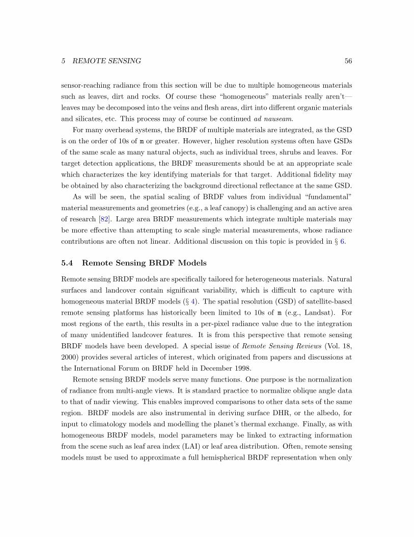
5 REMOTE SENSING 56

sensor-reaching radiance from this section will be due to multiple homogeneous materialssuch as leaves, dirt and rocks. Of course these “homogeneous” materials really aren’t—leaves may be decomposed into the veins and flesh areas, dirt into different organic materialsand silicates, etc. This process may of course be continued ad nauseam.

For many overhead systems, the BRDF of multiple materials are integrated, as the GSDis on the order of 10s of m or greater. However, higher resolution systems often have GSDsof the same scale as many natural objects, such as individual trees, shrubs and leaves. Fortarget detection applications, the BRDF measurements should be at an appropriate scalewhich characterizes the key identifying materials for that target. Additional fidelity maybe obtained by also characterizing the background directional reflectance at the same GSD.

As will be seen, the spatial scaling of BRDF values from individual “fundamental”material measurements and geometries (e.g., a leaf canopy) is challenging and an active areaof research [82]. Large area BRDF measurements which integrate multiple materials maybe more effective than attempting to scale single material measurements, whose radiancecontributions are often not linear. Additional discussion on this topic is provided in § 6.

5.4 Remote Sensing BRDF Models

Remote sensing BRDF models are specifically tailored for heterogeneous materials. Naturalsurfaces and landcover contain significant variability, which is difficult to capture withhomogeneous material BRDF models (§ 4). The spatial resolution (GSD) of satellite-basedremote sensing platforms has historically been limited to 10s of m (e.g., Landsat). Formost regions of the earth, this results in a per-pixel radiance value due to the integrationof many unidentified landcover features. It is from this perspective that remote sensingBRDF models have been developed. A special issue of Remote Sensing Reviews (Vol. 18,2000) provides several articles of interest, which originated from papers and discussions atthe International Forum on BRDF held in December 1998.

Remote sensing BRDF models serve many functions. One purpose is the normalizationof radiance from multi-angle views. It is standard practice to normalize oblique angle datato that of nadir viewing. This enables improved comparisons to other data sets of the sameregion. BRDF models are also instrumental in deriving surface DHR, or the albedo, forinput to climatology models and modelling the planet’s thermal exchange. Finally, as withhomogeneous BRDF models, model parameters may be linked to extracting informationfrom the scene such as leaf area index (LAI) or leaf area distribution. Often, remote sensingmodels must be used to approximate a full hemispherical BRDF representation when only

5 REMOTE SENSING 57

a few measurements are made, such as with a single pass of POLDER or or a few passesof an off-nadir viewing payload like MODIS (§ 3.5).

The general situation considered is a vegetative canopy region over a ground material.The canopy may have varying crown and leaf orientations, analogous to microfacet surfacevariations for homogeneous model. However, leafy materials have significant transmittanceand multiple interactions which complicate the radiometry. The vegetative canopy mayalso have varying spacing or areal density. A heavily forested region may have the entiresurface covered by tree crowns, with little ground visible, while other areas may have sparsetrees allowing the ground to drive the signature. Note that new commercial sources of highresolution (GSD ∼ 1 m) satellite imagery such as Space Imagingr and DigitalGlober haveenabled resolved surface features, providing a priori knowledge of the land cover type suchas “trees” or “grass.”

As with homogeneous material BRDF models, a range of empirical to physical modelshave been developed. Full empirical models are often not useful for satellite-derived ob-servations, since the geometric sampling density is very sparse. Physical models provideradiometric modelling of the surface and enable extraction of parameters having physicalsignificance. Finally, semi-empirical models provide a hybrid approach from which fits toempirical data provide some physical basis for the BRDF. Good reviews of remote sensingBRDF models are provided in an extensive treatment by Goel [83] which was summarizedand updated in [84]. Additional overviews of BRDF models are given by Strahler [85]and [86].

The discussion will be limited to semi-empirical models, which are often composed of asummation of linear contributions expressed as

fr(θi, θr, φ) =∑

n

anKn(θi, θr, φ) (70)

where n typically ranges from 2 to 10. Many models have n = 3 parameters with theKn terms consisting of isotropic, surface and volumetric functions. The Kn contributionsare called kernels from which these models are also called kernel-driven or kernel-basedmodels [86]. The kernels provide different geometric expressions for a particular typeof BRDF contribution. Detailed examination of a particular BRDF model by Roujeanprovides further details on the kernel representation.

The semi-empirical Roujean BRDF model [87] was among the first kernel-based modelsand has maintained popularity due to its versatility and accuracy for modelling a numberof land cover types. The BRDF is quantified by a geometric and volumetric scattering

5 REMOTE SENSING 58

component. The geometric scattering component models randomly placed vertical, opaque“long-wall protrusions” on a flat horizontal plane [87]. Both the protrusions and the back-ground plane are assumed to be Lambertian surfaces. Increasing zenith angle illuminationproduces increased shadowing of the background plane according to the protrusion height.However, the protrusions are distributed such that mutual shadowing of one protrusiononto another is not considered.

The volumetric component models randomly placed facets which absorb and scatterradiation according to a simple radiative transfer model. The facet distribution is treated asisotroptic, with a specified density. Several assumptions are made in deriving the volumetricterm—only single scattering is considered and the facet reflectance and transmittance aretreated as being equal. This last assumption is a gross one, but was necessary to reducethe number of free parameters in the model to three.

All scattering results from the geometric and volumetric components, which are con-sidered independent. The resulting BRDF model, is given by

fr(θi, θr, φ) = k0 + k1f1(θi, θr, φ) + k2f2(θi, θr, φ) (71)

where the geometric scattering results from k0 + k1f1 and the volumetric scattering iscontained in k2f2. Roujean used the function in terms of reflectance units, which is pro-portional to the BRDF (fr · 100π).

The f1 function is derived from geometric considerations of the protrusion placementand without further derviation is given by

f1 =12π

[(π − φ) cos φ + sinφ] tan θi tan θr

− 1π

(tan θi + tan θr +

√tan2 θi + tan2 θr − 2 tan θi tan θr cos φ

)(72)

The f2 function has its origin in a simple radiometry model, which includes some of thepreviously mentioned assumptions. It is given by

f2 =23π

(π − 2ξ) cos ξ + sin ξ

cos θi + cos θr− 1

3(73)

where ξ is the scattering angle between the incident and scattering directions (called thephase angle by some) defined by

cos ξ = cos θi cos θr + sin θi sin θr cos φ (74)

5 REMOTE SENSING 59

Figure 18: Roujean model results fit to empirical data for a wheat field in the visible forθi = 27, where the magnitude is normalized to reflectance units which replicates the resultsin [87, Fig. 7, p. 20,463]. The x-axis is θr and the y-axis is φ—note the principle plane isφ = 0 and φ = 180. (Ideally, this data would be presented in cylindrical coordinates foreasier interpretation). The peak reflectance is noted at the “hot spot” or retro-reflectionlocation. Parameter values are k0 = 27.3, k1 = 5.2 and k2 = 26.9.

Roujean’s convention is for 0 ≤ φ ≤ 180 and 0 ≤ θr ≤ 90, where the backscatteringorientation is φ = 0 (which is opposite the convention defined earlier where φ = 180 isthe backscattering orientation). The full derivation of these functions is lengthy, to whichthe reader may reference [87].

The free parameters, k0, k1 and k2 have some physical significance. k0 correlates toan isotropic Lambertian contribution and is equivalent to the reflectance when θi = θr =0. k1 is related to the protrusion height, length and width while k2 is related to thefacet reflectance and area (e.g., canopy leaf reflectance and coverage, or leaf area index).The model was implemented in a computer program, and some of Roujean’s results arereplicated from parameters in the paper as seen in Figure 18.

5.5 Remote Sensing BRDF Model Performance

The performance of several BRDF models, most of which are remote sensing models, isreported by Boucher [30] and Hautecoeur [88]. Boucher made measurements on sand, “dry”grass, and “green” grass at 600 and 800 nm. Significant in this work is the quantification

5 REMOTE SENSING 60

of model performance for different azimuth sampling densities. The Roujean model [87]provided one of the best performances, and had minimal errors for all the materials at bothwavelengths when at least 25 hemispherical samples were acquired (for a single θi value).The Roujean model also provided good performance when measurements were limited toonly three azimuth planes: φ = 0 (or 180), 60 and 120. Roujean’s model was alsocommended by Hautecoeur [88], having the best performance of the semi-empirical modelssurveyed.

5.6 Old vs. new “yellow school buses”

Sad to say, but once BRDF data and models are in place for employment in spectralalgorithms, the job is only partially complete (though what a job it was). More oftenthan not, the BRDF characterization for material X does not represent material X in thefield. Weathering of the material alters the optical properties via UV “washing,” oxidation,surface abrasions, etc. Also, the material may be covered by dust and other particulates—or perhaps mud for tactical military vehicles. A cursory examination of these effects hasbeen made by Thomas [89].

It’s worth noting that since material weathering and/or degradation impacts the BRDF,it also impacts the general “reflectance” of a material [Eq (13)]. This is readily apparent byvisual inspection of materials. The result is that algorithms using simple spectral reflectanceare also impacted.

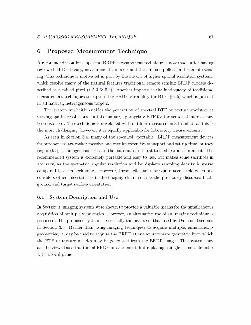
6 PROPOSED MEASUREMENT TECHNIQUE 61

6 Proposed Measurement Technique

A recommendation for a spectral BRDF measurement technique is now made after havingreviewed BRDF theory, measurements, models and the unique application to remote sens-ing. The technique is motivated in part by the advent of higher spatial resolution systems,which resolve many of the natural features traditional remote sensing BRDF models de-scribed as a mixed pixel (§ 5.3 & 5.4). Another impetus is the inadequacy of traditionalmeasurement techniques to capture the BRDF variability (or BTF, § 2.5) which is presentin all natural, heterogeneous targets.

The system implicitly enables the generation of spectral BTF or texture statistics atvarying spatial resolutions. In this manner, appropriate BTF for the sensor of interest maybe considered. The technique is developed with outdoor measurements in mind, as this isthe most challenging; however, it is equally applicable for laboratory measurements.

As seen in Section 3.4, many of the so-called “portable” BRDF measurement devicesfor outdoor use are rather massive and require extensive transport and set-up time, or theyrequire large, homogeneous areas of the material of interest to enable a measurement. Therecommended system is extremely portable and easy to use, but makes some sacrifices inaccuracy, as the geometric angular resolution and hemisphere sampling density is sparsecompared to other techniques. However, these deficiencies are quite acceptable when oneconsiders other uncertainties in the imaging chain, such as the previously discussed back-ground and target surface orientation.

6.1 System Description and Use

In Section 3, imaging systems were shown to provide a valuable means for the simultaneousacquisition of multiple view angles. However, an alternative use of an imaging technique isproposed. The proposed system is essentially the inverse of that used by Dana as discussedin Section 3.3. Rather than using imaging techniques to acquire multiple, simultaneousgeometries, it may be used to acquire the BRDF at one approximate geometry, from whichthe BTF or texture metrics may be generated from the BRDF image. This system mayalso be viewed as a traditional BRDF measurement, but replacing a single element detectorwith a focal plane.

6 PROPOSED MEASUREMENT TECHNIQUE 62

6.1.1 FOV and standoff distance determination

Imaging with a narrow field of view (FOV) camera produces the equivalent of a singleBRDF measurement. The BRDF of a sample imaged in this manner is directly proportionalto the average irradiance across the focal plane, or the average digital count (DC) valuefor a spectral band across the focal plane. Positioning and imaging with the camera atlocations in the scattering hemisphere provides geometric coverage in the same manneras a single detector. The high frequency or texture variation is manifested in the detailscaptured at levels less than the full frame of the camera down to the individual pixel orinstantaneous field of view (IFOV, more on this below). The angular resolution of theBRDF measurement, ∆θr and ∆φr is therefore limited by and equivalent to the cameraFOV.

The selection criteria for an appropriate FOV is a function of three interrelated criteria:

1. minimizing the angular resolution, ∆θr and ∆φr,

2. maximizing the spatial extent or ground field of view (GFOV) of sample measurementand

3. a reasonable camera to sample distance for ease of repositioning and adjustments.

The importance of criteria 1 is determined by the magnitude of the derivative of the BRDFwith respect to θr and φr. Significant changes in the BRDF are characteristic of specularmaterials near the specular lobe. Fortunately, most natural materials in the VNIR are notappreciably specular.

The sample size (criteria 2) is determined by the variation or texture scale of thatmaterial. For instance, a painted automobile surface may have the texture sufficientlyaveraged out over a 1 in × 1 in area, while grass may require 1 ft × 1 ft area and shrubsa 10 ft × 10 ft.

Criteria 3, the camera to sample distance, will mostly drive the ease of repositioningthe camera in the hemisphere above the sample. While an increased standoff distance mayresult in decreasing ∆θr and ∆φr and/or potential increases in the spatial area measured, itmay become increasingly difficult to transport and quickly set up the system. Easy accessto the camera at all hemispherical positions would limit this distance to ∼ 6 ft.

A qualitative estimate of a good compromise of these variables is a camera having a10 (full angle) FOV. For nadir viewing (θr = 0) of a sample from a distance of 6 ft,this corresponds to a GFOV ≈ 1 ft × 1 ft. This configuration is estimated to covermost measurements of interest. If this measurement area is not adequate for a material

6 PROPOSED MEASUREMENT TECHNIQUE 63

to be sufficiently homogeneous, then multiple series of measurements may be made byrepositioning the system. Alternatively, an increased standoff distance may be used. At theopposite extreme, materials which are highly specular may require the use of an alternatelens which reduces the FOV.

6.1.2 Radiance calibrations

Calibration of radiance levels will be ensured by characterizing the camera response fornonlinearities and imaging a Spectralonr or pressed halon calibration surface prior to andafter each measurement. Being a perfectly (or nearly so) Lambertian surface with ρ(λ) / 1,the BRDF of the halon will be / 1

π sr−1. However, measurement of the calibration targetwill also contain contributions from the scattered downwelled skydome radiance.

The sky radiance may not be eliminated, but the direct solar irradiance may. Imagingthe calibration target when in shadow from the sun will provide a measure of the downwelledradiance contributions. Therefore, the radiance received in full sun and when illuminatedby the sky, minus the radiance with only the sky results in reflection due to the directsolar radiance. In terms of digital counts, deriving the Lambertian BRDF in this manneris expressed as

DCLamb = DCsky+sun −DCsky−sun = π−1 [sr−1] (75)

The initial measurement and camera exposure adjustments should be made at the geometrywhere the signature is greatest in order to ensure the dynamic range of the camera is notexceeded on subsequent measurements, as changes in the camera response/exposure settingsare not desired.

A sample image of grass acquired using this measurement technique is now discussedand used as an example (Figure 19). An arbitrary GSD unit is also shown in the figureand will be used for subsequent discussion on texture and the adequacy of the image tocapture the BRDF. The sample or image is ∼ 1 ft across making the representative GSDunit approximately 3 in.

6.1.3 Hemispherical sampling strategy

Any strategy devised for sampling the hemisphere above the material must consider thetotal time required to complete all measurements. Depending on the latitude and timeof year, the sun has an apparent angular rate of up to 15/hr. Changes in the incidentsolar angle should be kept less than or commensurate with the reflection angle resolution(FOV) or ∆θr ≈ ∆φ ≈ 10. For materials with azimuthal symmetry, only changes in

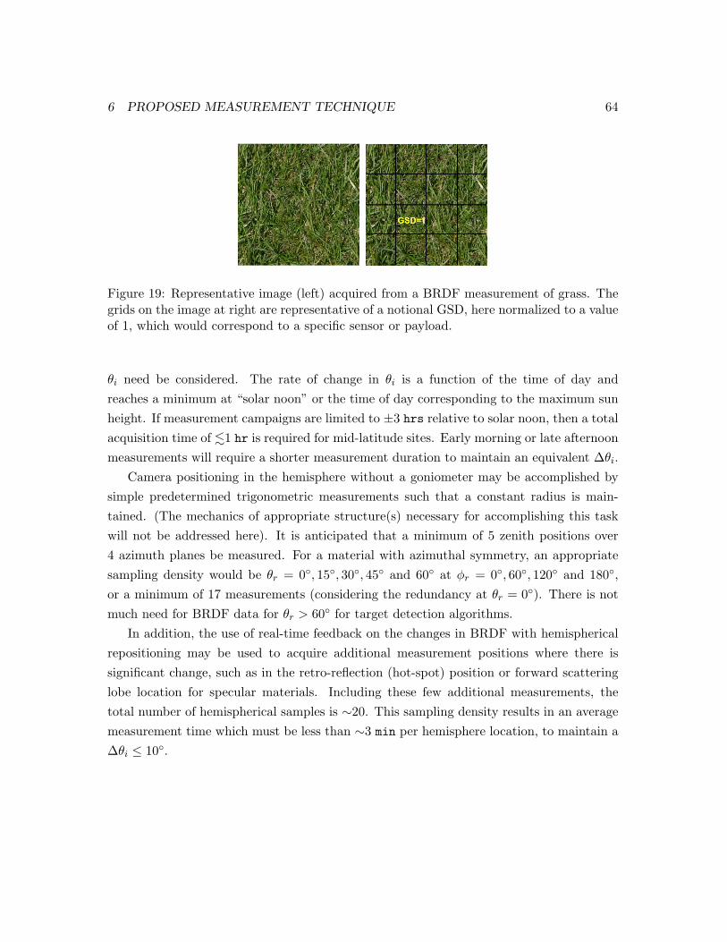
6 PROPOSED MEASUREMENT TECHNIQUE 64

Figure 19: Representative image (left) acquired from a BRDF measurement of grass. Thegrids on the image at right are representative of a notional GSD, here normalized to a valueof 1, which would correspond to a specific sensor or payload.

θi need be considered. The rate of change in θi is a function of the time of day andreaches a minimum at “solar noon” or the time of day corresponding to the maximum sunheight. If measurement campaigns are limited to ±3 hrs relative to solar noon, then a totalacquisition time of .1 hr is required for mid-latitude sites. Early morning or late afternoonmeasurements will require a shorter measurement duration to maintain an equivalent ∆θi.

Camera positioning in the hemisphere without a goniometer may be accomplished bysimple predetermined trigonometric measurements such that a constant radius is main-tained. (The mechanics of appropriate structure(s) necessary for accomplishing this taskwill not be addressed here). It is anticipated that a minimum of 5 zenith positions over4 azimuth planes be measured. For a material with azimuthal symmetry, an appropriatesampling density would be θr = 0, 15, 30, 45 and 60 at φr = 0, 60, 120 and 180,or a minimum of 17 measurements (considering the redundancy at θr = 0). There is notmuch need for BRDF data for θr > 60 for target detection algorithms.

In addition, the use of real-time feedback on the changes in BRDF with hemisphericalrepositioning may be used to acquire additional measurement positions where there issignificant change, such as in the retro-reflection (hot-spot) position or forward scatteringlobe location for specular materials. Including these few additional measurements, thetotal number of hemispherical samples is ∼20. This sampling density results in an averagemeasurement time which must be less than ∼3 min per hemisphere location, to maintain a∆θi ≤ 10.

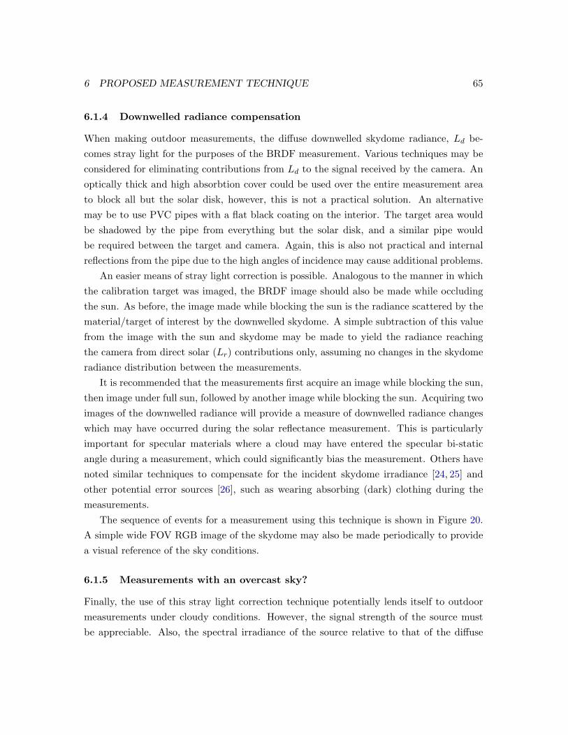
6 PROPOSED MEASUREMENT TECHNIQUE 65

6.1.4 Downwelled radiance compensation

When making outdoor measurements, the diffuse downwelled skydome radiance, Ld be-comes stray light for the purposes of the BRDF measurement. Various techniques may beconsidered for eliminating contributions from Ld to the signal received by the camera. Anoptically thick and high absorbtion cover could be used over the entire measurement areato block all but the solar disk, however, this is not a practical solution. An alternativemay be to use PVC pipes with a flat black coating on the interior. The target area wouldbe shadowed by the pipe from everything but the solar disk, and a similar pipe wouldbe required between the target and camera. Again, this is also not practical and internalreflections from the pipe due to the high angles of incidence may cause additional problems.

An easier means of stray light correction is possible. Analogous to the manner in whichthe calibration target was imaged, the BRDF image should also be made while occludingthe sun. As before, the image made while blocking the sun is the radiance scattered by thematerial/target of interest by the downwelled skydome. A simple subtraction of this valuefrom the image with the sun and skydome may be made to yield the radiance reachingthe camera from direct solar (Lr) contributions only, assuming no changes in the skydomeradiance distribution between the measurements.

It is recommended that the measurements first acquire an image while blocking the sun,then image under full sun, followed by another image while blocking the sun. Acquiring twoimages of the downwelled radiance will provide a measure of downwelled radiance changeswhich may have occurred during the solar reflectance measurement. This is particularlyimportant for specular materials where a cloud may have entered the specular bi-staticangle during a measurement, which could significantly bias the measurement. Others havenoted similar techniques to compensate for the incident skydome irradiance [24, 25] andother potential error sources [26], such as wearing absorbing (dark) clothing during themeasurements.

The sequence of events for a measurement using this technique is shown in Figure 20.A simple wide FOV RGB image of the skydome may also be made periodically to providea visual reference of the sky conditions.

6.1.5 Measurements with an overcast sky?

Finally, the use of this stray light correction technique potentially lends itself to outdoormeasurements under cloudy conditions. However, the signal strength of the source mustbe appreciable. Also, the spectral irradiance of the source relative to that of the diffuse

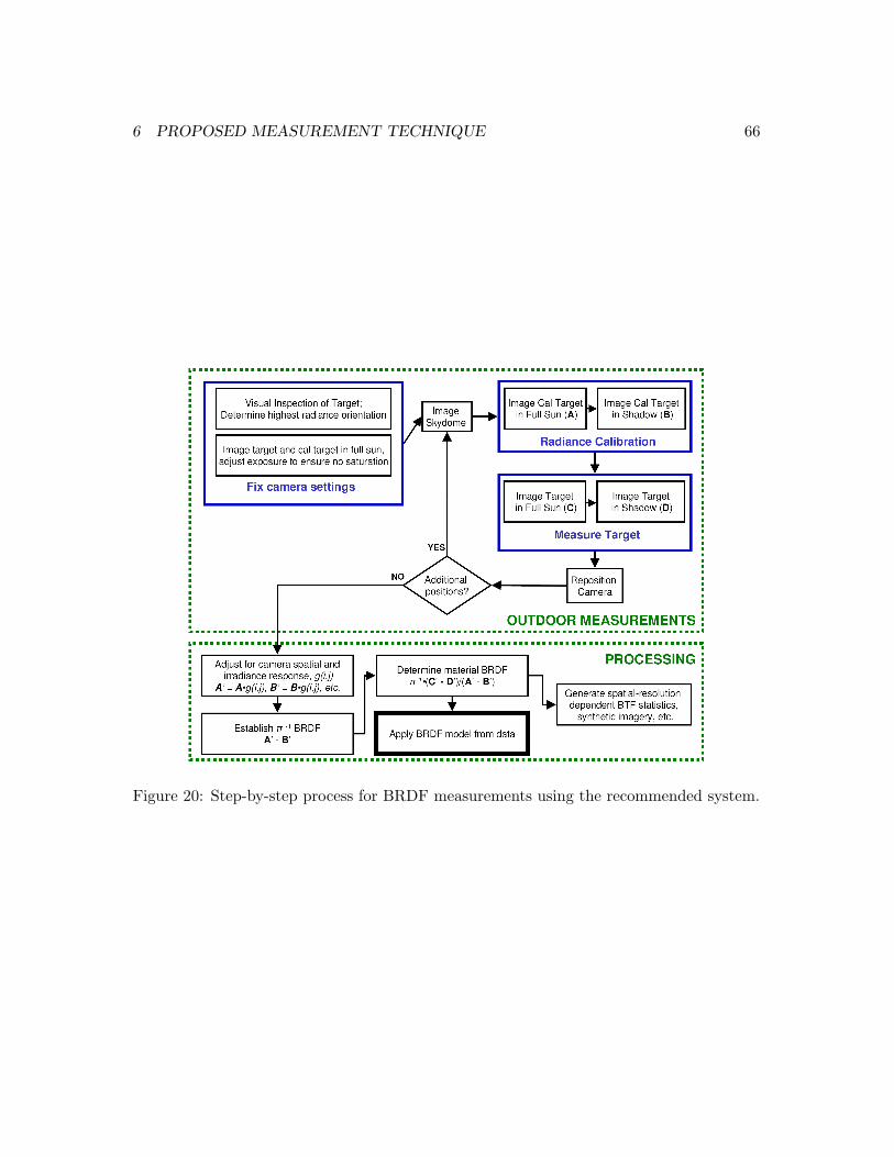
6 PROPOSED MEASUREMENT TECHNIQUE 66

Figure 20: Step-by-step process for BRDF measurements using the recommended system.

6 PROPOSED MEASUREMENT TECHNIQUE 67

skydome needs to be considered. The incident irradiance on the target area should begreater than or equal to the solar insolation, which is approximately 1 kW/m2. For thenotional 10 FOV setup previously described, the incident VNIR power in the target areashould be greater than 100 W. Higher spectral irradiance values than that delivered by thesun will improve the measurements relative to those that may be made with the sun.

Often cloud cover is not dense, which results in a temporally varying magnitude ofdirect solar irradiance incident upon the target. In these circumstances, alignment of theillumination source adjacent to the solar incidence angle is recommended.

A better solution to competing with the diffuse sky radiance is to make the measure-ments at night. Calibration of stray light may still be required if nearby illuminants arepresent and the source signal is modest. Even at night, irradiance uniformity over the tar-get and divergence of the irradiance source from a planar field are additional complicationswhich must be managed.

6.2 GSD Sample Statistics Generation

The measurement technique described above readily lends itself to derivation of the textureor BTF statistics which may be used in algorithms and rendering synthetic imagery. Forexample, consider the GSD unit in Figure 19, (which in reality is approximately 3 in). Thevariability or texture of this grass material for a system having a GSD=1 may be derivedby examining the moving average statistics of the area underneath this GSD=1 square.This is mathematically equivalent to convolution which is given as

g[x, y] = f [x, y] ∗ h[x, y] =∫∫ +∞

−∞f [α, β] h[x− α, y − β] dα dβ (76)

where f [x, y] is the image and h[x, y] is the convolution kernel. For the case of a digitalimage with pixels (i.e, non-continuous), the discrete convolution is

g[x, y] =1

X2

m−1∑i=0

n−1∑j=0

f [x, y] h[x− i, y − j] (77)

For simple local averaging, the convolution kernel is a square of size X ×X pixels corre-sponding to the fractional GSD of interest. The convolution kernel has a magnitude of “1”everywhere inside the GSD box and zero outside (i.e., RECT function). The 1

X2 factor inEq. (77) compensates for the summed values of the kernel and hence enables the equation

6 PROPOSED MEASUREMENT TECHNIQUE 68

Figure 21: Local averaging with the image used for BRDF statistics generation. At leftis the original 400 × 400 (GSD=0.01) image followed by images averaged to 40 × 40(GSD=0.1), 10 × 10 (GSD=0.4), 4 × 4 (GSD=1.0) and 1 × 1 (GSD=4.0).

to return the DC value of the area under the kernel. Note that a simple RECT functionis used here, but the actual point spread function (PSF) of the imaging system in questionmay be used to provide a sensor-specific BTF.

Using this approach, BTF statistics may be generated from a BRDF image. Considerthe 400 × 400 pixel image of grass shown in Figure 19. If a GSD of 1 is defined as a 100× 100 area of the image, a convolution kernel of this GSD size may be used to generate animage, g[x, y], of local averaged values. The size of g[x, y] is determined by the size of theconvolution kernel and original image. For a convolution kernel of 100 × 100 as previouslydiscussed, g[x, y] will be 400-100+1 or 301 × 301. Increasing the GSD of interest willresult in more averaging, while decreasing will result in more variability. For instance, ifthe convolution kernel were the same size as the original image, then a single value (pixel)corresponding to the global image average would be returned. At the other extreme, aconvolution kernel of 1 × 1 would return the original image. By this means, the texture orBTF information (§ 2.5) may be extracted directly from the image.

Figure 21 provides a direct representation of this process. The original image usedto determine “grass” BRDF is shown at left. The other images correspond to increasedaveraging by selection of different GSD scales. Note that the averaging shown here is fornon-overlapping, contiguous GSD regions, whereas the statistics generated by the convo-lution are done for overlapping GSD regions. The far right of Figure 21 is the average forthe entire image, and is proportional to the BRDF value for this measurement. In thiscase, the average digital count value for the R, G and B channels is 78.86, 94.40 and 33.31,respectively.

Using the convolution approach for texture statistics, histograms or equivalently theBRDF probability distribution may be generated as a function of GSD for each acquiredimage which corresponds to a unique solar zenith angle (θi) and viewing geometry (θr, φ).

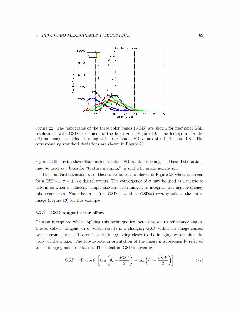
6 PROPOSED MEASUREMENT TECHNIQUE 69

Figure 22: The histograms of the three color bands (RGB) are shown for fractional GSDresolutions, with GSD=1 defined by the box size in Figure 19. The histogram for theoriginal image is included, along with fractional GSD values of 0.1, 1.0 and 1.8. Thecorresponding standard deviations are shown in Figure 23.

Figure 22 illustrates these distributions as the GSD fraction is changed. These distributionsmay be used as a basis for “texture mapping” in synthetic image generation.

The standard deviation, σ, of these distributions is shown in Figure 23 where it is seenfor a GSD=1, σ = ± ∼5 digital counts. The convergence of σ may be used as a metric todetermine when a sufficient sample size has been imaged to integrate out high frequencyinhomogeneities. Note that σ → 0 as GSD → 4, since GSD=4 corresponds to the entireimage (Figure 19) for this example.

6.2.1 GSD tangent error effect

Caution is required when applying this technique for increasing zenith reflectance angles.The so called “tangent error” effect results in a changing GSD within the image causedby the ground in the “bottom” of the image being closer to the imaging system than the“top” of the image. The top-to-bottom orientation of the image is subsequently referredto the image y-axis orientation. This effect on GSD is given by

GSD = R · cos θr

[tan

(θr +

FOV

2

)− tan

(θr −

FOV

2

)](78)

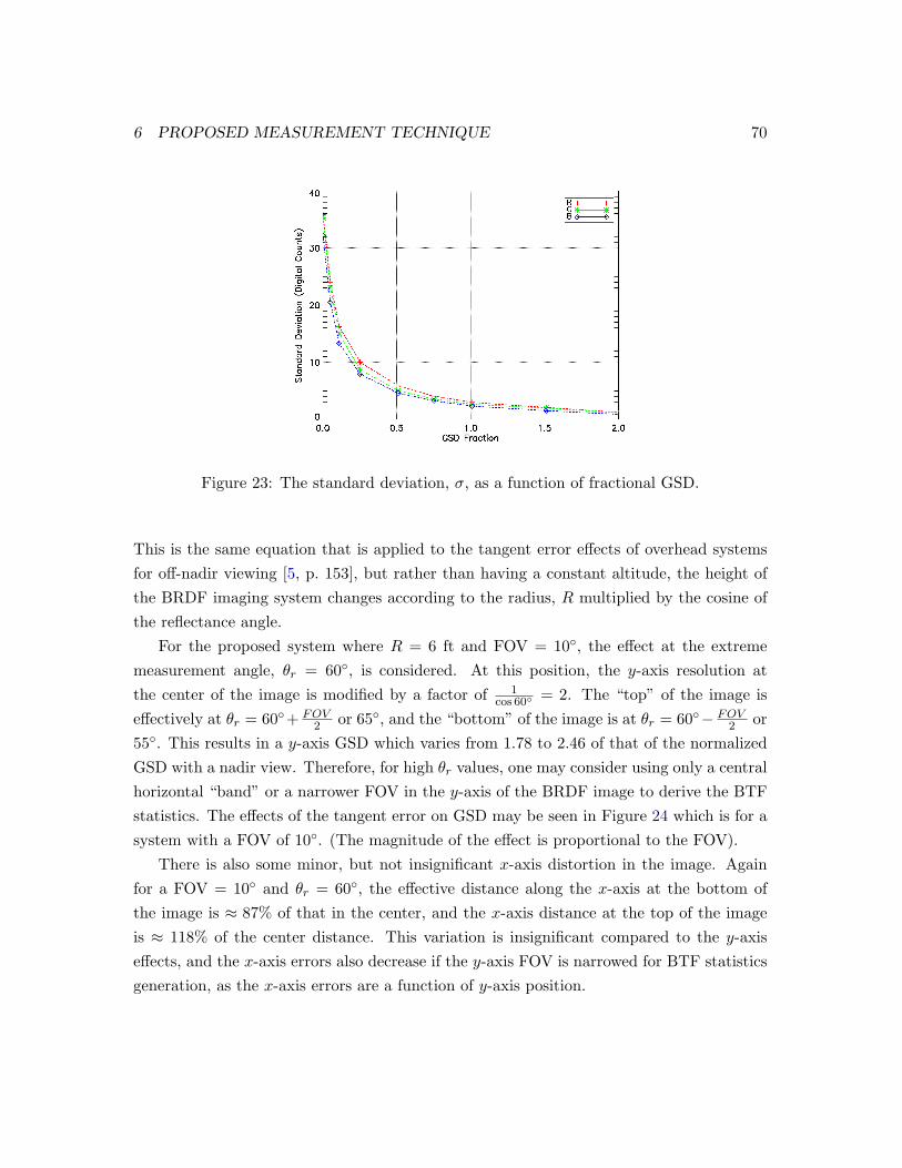
6 PROPOSED MEASUREMENT TECHNIQUE 70

Figure 23: The standard deviation, σ, as a function of fractional GSD.

This is the same equation that is applied to the tangent error effects of overhead systemsfor off-nadir viewing [5, p. 153], but rather than having a constant altitude, the height ofthe BRDF imaging system changes according to the radius, R multiplied by the cosine ofthe reflectance angle.

For the proposed system where R = 6 ft and FOV = 10, the effect at the extrememeasurement angle, θr = 60, is considered. At this position, the y-axis resolution atthe center of the image is modified by a factor of 1

cos 60 = 2. The “top” of the image iseffectively at θr = 60+ FOV

2 or 65, and the “bottom” of the image is at θr = 60− FOV2 or

55. This results in a y-axis GSD which varies from 1.78 to 2.46 of that of the normalizedGSD with a nadir view. Therefore, for high θr values, one may consider using only a centralhorizontal “band” or a narrower FOV in the y-axis of the BRDF image to derive the BTFstatistics. The effects of the tangent error on GSD may be seen in Figure 24 which is for asystem with a FOV of 10. (The magnitude of the effect is proportional to the FOV).

There is also some minor, but not insignificant x-axis distortion in the image. Againfor a FOV = 10 and θr = 60, the effective distance along the x-axis at the bottom ofthe image is ≈ 87% of that in the center, and the x-axis distance at the top of the imageis ≈ 118% of the center distance. This variation is insignificant compared to the y-axiseffects, and the x-axis errors also decrease if the y-axis FOV is narrowed for BTF statisticsgeneration, as the x-axis errors are a function of y-axis position.

6 PROPOSED MEASUREMENT TECHNIQUE 71

Figure 24: GSD tangent error effects with increasing θr for a system with an FOV of 10.The results are normalized to the nadir view where the solid (red) line corresponds to they-axis GSD at the center of the image, and the dashed (blue) line is the difference betweenthe top and bottom of the image or y-axis extremes.

6.2.2 Image mis-registration errors

Another area of concern is registration of the two images made to correct for the downwelledsky radiance: 1) the image made with sun and sky illuminating the target and 2) thatwith only the sky radiance illuminating the target. Depending on the stability of thecamera mount and the weather and target conditions (e.g., tall grass in wind), significantBTF statistic errors may be present from the subtraction of the mis-registered calibrationimages. Note that these errors are limited to BTF metrics, and do not affect the BRDFdetermination. The errors may become appreciable as the GSD size (or convolution kernel)decreases to the fidelity of the image registration. With a reasonably sized focal plane(> 256 × 256), this should only become an issue for GSD sizes less than 1

100 of the imagesize, unless wind is appreciably moving the target, which may become an issue for tallgrass.

6.2.3 Spectral correlation

To faithfully reproduce the spectral BTF using the aforementioned technique, another levelof fidelity is required. The spectral values for each pixel are not statistically independent,but are correlated. Therefore, simply generating a spectral BRDF based upon the individ-ual band probability distributions shown in Figure 22 is not sufficient. Spectral errors are

6 PROPOSED MEASUREMENT TECHNIQUE 72

Figure 25: Synthetically-generated grass images using the original image (Figure 19) statis-tics with no spectral correlation. Spectral errors are evident (with a color copy). The leftimage is generated from a GSD equivalent to 1 pixel in the original image, while the rightimage is generated from a GSD=1 unit as presented in Figure 19. The images are only a20× 20 section so that individual pixels are discernable.

evident when band-to-band correlation is not considered, as illustrated by Figure 25. Theoccurrence of the predominantly blue pixels in the figure is easily understood by inspectionof the histogram of the original image (Figure 22), where it is seen that random selectionof a high blue value may be accompanied by lower red and green values. To first order,most of the correlation is simply a change in the magnitude or a DC shift across all spectralvalues; however, the spectral shape may also change depending on other unique conditions.

The covariance matrix between bands may be used to capture the band-to-band spectraldependencies. However, when several random variables are considered, the process is noteasily managed as the dimensions of the covariance matrix increases to the number ofrandom variables. For hyperspectral images, generation of a ∼100+ dimensional covariancehypercube is not feasible.

An alternate technique of maintaining the spectral correlation is to begin with onespectral band (band 1) and generate a random value per that band’s probability densityfunction, fi(DC). Then, the distribution of the next band (band 2) will be altered bythe conditional probability based upon the value selected for band 1. The new probabilitydensity for band 2 will then be used to generate that band’s value. This process continuesuntil all bands have been selected. This technique should provide an improvement overthe Single-Bandpass (SBP) Z-score algorithm used in DIRSIG, which essentially selects anappropriate spectral vector given the average value over a narrow spectral band [90].

A potential pitfall of this method is having too many spectral bands for the spatialdimension of the image. Each band selection narrows the population available for the next

6 PROPOSED MEASUREMENT TECHNIQUE 73

band’s selection. If a sparse population (or no population) is left for selection of the lastband, then the bin size of the bands may be increased which will enable a larger survivingpopulation. This technique becomes crucial as one considers high dynamic range sensorhaving 10 or more bits. Consider a hypothetical case of a 1000× 1000 10-bit spatial imagewith 10 spectral bands. Assume a uniform distribution for each band. Given 1024 valuesavailable, the first band selected would each have 10002

1024 or approximately 1000 pixels perdigital count value. Selection of a single digital count value would only leave 1000 pixelsleft to determine the subsequent band’s distribution. One quickly exhausts the availablepopulation of pixels from which statistical draws may be made. Increasing the bin sizearound the selected digital count provides a means of alleviating this problem, with minimalaccuracy sacrificed.

This technique was implemented in a computer algorithm and found to be effective, butvery slow. Even with more efficient coding, it is doubtful this technique will be fast enoughfor hardware in the near future. An alternative approach is to provide a much coarserapproximation which is still effective. Rather than maintaining the spectral probabilitydensity function at the resolution of single digital count values, the PDF may be dividedinto much more coarse bins across the dynamic range of the system. For instance, fivedivisions per distribution would allow bands having 20% of the population in each group.

Using such a division, the condition probabilities may be computed once and storedin two multi-dimensional arrays: one having the mean values and the other having thevariance. The number of dimensions will equal the number of bands, i, which results in thetotal number of elements in each matrix equal to 5i. For three bands such as used in thisexample, this is manageable. However, as with the first technique, once a realistic numberof bands are considered, an unrealistic magnitude results. Principal components analysismay then be used to reduce the dimensionality of the data to a manageable number (< 10).For producing the remaining bands, it is suggested to use their mean and variance withoutconsideration of conditional probability.

After having accounted for the spectral correlation, it should be noted that spatialcorrelation or texturing effects at a level greater than a single pixel have not been considered.This becomes important if one uses hyperspectral algorithms which consider the spatialextent of features, such as the RX algorithm [91]. Realistic spatial texture generation hasbeen and will continue to be an active area of research [90].

6 PROPOSED MEASUREMENT TECHNIQUE 74

6.3 Hemispherical interpolation

Having seen the significant research invested in deriving BRDF models, one feels compelledto apply an appropriate model(s) to the acquired data. However, simple empirical inter-polation of the measured values is recommended as performed by Sandmeier (§ 4.2). Thisis driven by two considerations: 1) the density of the hemispherical sampling using therecommended technique is sufficient to provide a reasonable estimate of BRDF given theother uncertainties in the imaging chain and 2) application of models is highly dependentupon the particular material type. One model is not likely to provide accurate results forall ranges of material types measured.

Some means of extrapolating to other solar incident angles, θi, must be used. A semi-empirical heterogeneous model, such as Roujean’s model (§ 5.4), is recommended for naturaltargets. For highly homogeneous (typically man-made) targets, a homogeneous BRDFmodel may provide improvements to other θi positions. However, these materials are oftensuitable for lab measurements which are not constrained by the sun position for various θi

measurements.The volume of data is limited to ∼ 20 images per θi, and the number of θi values will

likely be less than three. So the raw data notionally consists of 20–60 images. For a 256 ×256 focal plane having a 16 bit dynamic range, each spectral band for each image will be∼ 130 KB. Considering a range of 3 to 100 for the number of spectral bands, along with thetotal number of images for each material, the entire data set for a material would thereforeconsist of 7.8–780 MB.

6.4 Spectral Interpolation

Ideally, one would like to employ the described BRDF imaging system with a hyperspectralimaging system having contiguous spectral coverage with resolution of < ∆λ = 10 nm. Ifsuch a system is used, spectral interpolation may not be required; however, it is likely thatsuch a robust system is not available or impractical due to signal to noise considerations.

In the event one is left with a spectrally modest system, an efficient and accurate meansof providing detailed spectral coverage is required. One candidate technique is to use a non-imaging spectrometer which has a FOV approximately the same as the imaging system.Other techniques, such as that used by the NEF database, make the reasonable assumptionthat the spectral-dependent variance in the BRDF is proportional to the variance in theDHR for that wavelength.

6 PROPOSED MEASUREMENT TECHNIQUE 75

6.5 Polarized Measurements

Determination of the Mueller matrix, Mr, is possible using this system according to themeasurement protocol described in § 3.6. Lab measurements using such a technique arerelatively straightforward, but outdoor measurements using this technique are problematic.Polarization filters would have to be positioned between the sun and target for the mea-surements, and the number of required measurements would likely not be completed in atime reasonable to maintain reasonable accuracy in the solar zenith position, θi.

However, the use of linear filters over the camera enables derivation of the Stokesparameters, which enables derivation of the first column of the BRDF Mueller matrix. Thisis an adequate descriptor when illumination sources are randomly polarized. However, thedownwelled radiance of the skydome is polarized by atmospheric scatter. There is stillsome utility in acquiring Stokes BRDF images, since the direct solar illumination oftenexceeds 80% of the incident irradiance onto materials, and of the remaining 20% skydomediffuse irradiance, less than 5% (or one quarter) in a weighted-average sense is estimatedto be comprised of linearly polarized radiance. A much more significant contributor to thepolarized signature may be the upwelled radiance (~Lu, Eq 68c) along the target to sensorpath. These sensitivities are a topic for further study by the author.

7 CONCLUSION 76

7 Conclusion

The bidirectional reflectance distribution function (BRDF) has been examined in detail.Electromagnetic theory fundamentally describes the interaction of light with matter, andthe BRDF may be used to characterize the reflected radiance for real materials. An array ofmeasurement techniques have been examined. Significant advances in BRDF measurementhave been enabled by the use of focal plane arrays. Models are still required to effectivelyrepresent BRDF, as there are an infinite number of measurements to fully quantify BRDF.Physical parameters of interest may also be derived by fitting empirical data to BRDFmodels. Remote sensing requirements for BRDF may be understood by examining theindividual radiance contribution components reaching a sensor aperture. BRDF data pro-vides for the normalization of multiple views, and improves quantitative remote sensingalgorithm performance.

A BRDF measurement technique has been recommended that provides the ability toquantify the BRDF variance or texture within natural materials. This is particularlyimportant for high-resolution systems. The measurement technique inherently providesa means to derive texture statistics, which may be tailored to a particular sensor’s pointspread function.

REFERENCES 77

References

[1] J. H. Lambert. Photometria sive de mensura et grabibusluminis, colorum et umbrae. Technical report, Augsberg,Germany, 1760.

[2] Kinsell L. Coulson. Polarization and Intensity of Light inthe Atmosphere. A. DEEPAK Publishing, 1988.

[3] Robert D. Guenther. Modern Optics. John Wiley & Sons,1990.

[4] Eugene Hecht. Optics. Addison-Wesley, second edition,1987.

[5] John R. Schott. Remote Sensing: The Image Chain Ap-proach. Oxford University Press, 1997.

[6] Harold B. Westlund and Gary W. Meyer. The role ofrendering in the competence project in measurement sci-ence for optical reflection and scattering. Journal of Re-search of the National Institute of Standards and Technol-ogy, 107(3):247–259, May-June 2002.

[7] F. E. Nicodemus. Reflectance nomenclature and di-rectional reflectance and emissivity. Applied Optics,9(6):1474–1475, June 1970.

[8] F. E. Nicodemus, J. C. Richmond, J. J. Hsia, I. W. Gins-berg, and T. Limperis. Geometrical considerations andnomenclature for reflectance; NBS Monograph 160. Tech-nical report, Department of Commerce, National Bureauof Standards, 1977.

[9] Kristin J. Dana, Bram van Ginneken, Shree K. Nayar, andJan J. Koenderink. Reflectance and texture of real-worldsurfaces. ACM Transactions on Graphics (TOG), 18(1):1–34, January 1999.

[10] W. Ni, C. E. Woodcock, and D. L. B. Jupp. Variance inbidirectional reflectance over discontinuous plant canopies.Remote Sensing of Environment, 69(1):1–15, July 1999.

[11] John C. Stover. Optical Scattering Measurement and Anal-ysis. SPIE Optical Engineering Press, second edition,1995.

[12] D. S. Flynn and C. Alexander. Polarized surface scatteringexpressed in terms of a bidirectional reflectance distribu-tion function matrix. Optical Engineering, 34:1646–1650,1995.

[13] George Borshukov. Measured BRDF in film production—realistic cloth appearance for The Matrix Reloaded. Inter-net, 2004.

[14] Phillip R. Mattison, Mark S. Dombrowski, James M.Lorenz, Keith J. Davis, Harley C. Mann, Philip Johnson,and Bryan Foos. Handheld directional reflectometer: anangular imaging device to measure BRDF and HDR in realtime. volume 3426. SPIE, 1998.

[15] Michael T. Beecroft and Phillip R. Mattison. Design re-view of an in-situ bidirectional reflectometer. In Scatteringand Surface Roughness, volume 3141 of Proc. SPIE, pages196–208, 1997.

[16] Xiaofan Feng. Comparison of methods for generation ofabsolute reflectance factor measurements for BRDF stud-ies. Master’s thesis, Rochester Institute of Tchnology,1990.

[17] S. R. Sandmeier and A. H. Strahler. BRDF laboratorymeasurements. Remote Sensing Reviews, 18(2–4):481–502,September 2000.

[18] Stephen R. Marschner, Stephen H. Westin, Eric P. F.Lafortune, Kenneth E. Torrance, and Donald P. Green-berg. Image-based BRDF measurement including humanskin. In Eurographics Workshop on Rendering, 1999.

[19] K.J. Dana. BRDF/BTF measurement device. In EighthIEEE International Conference on Computer Vision, vol-ume 2, pages 460–466. IEEE, July 2001.

[20] Kristin J. Dana and Jing Wang. Device for convenientmeasurement of spatially varying bidirectional reflectance.JOSA A, 21(1):1–12, January 2004.

[21] Oliver Apel, Christian Goerling, Uwe Leinhos, Klaus R.Mann, and Bernd Schaefer. CHARISMA: a new wayfor angular-resolved scattering measurements. In Laser-Induced Damage in Optical Materials, volume 4347 ofProc. SPIE, pages 569–578, 2001.

[22] Jefferson Y. Han and Ken Perlin. Measuring bidirectionaltexture reflectance with a kaleidoscope. ACM Transactionson Graphics (TOG), 22(3):741–748, July 2003.

[23] Charles Walthall, Jean-Louis Roujean, and Jeff Morisette.Field and landscape BRDF optical wavelength measure-ments: Experience, techniques and the future. RemoteSensing Reviews, 18:503–531, 2000.

[24] Stefan R. Sandmeier. Acquisition of bidirectional re-flectance factor data with field goniometers. Remote Sens-ing of Environment, 73(3):257–269, September 2000.

[25] A. I. Lyapustin and J. L. Privette. A new method of re-trieving surface bidirectional reflectance from ground mea-surements: Atmospheric sensitivity study. Journal of Geo-physical Research, 104(D6):6257–6268, March 27 1999.

[26] G. F. Epema. Studies of errors in field measurements ofthe bidirectional reflectance factor. Remote Sensing of theEnvironment, 35:37–49, 1991.

[27] S. Sandmeier, W. Sandmeier, K.I. Itten, M.E. Schaepman,and T.W. Kellenberger. The Swiss field-goniometer system(FIGOS). In International Geoscience and Remote SensingSymposium, volume 3 of Proc. IEEE, pages 2078–2080,1995.

REFERENCES 78

[28] S. R. Sandmeier and K. I. Itten. A field goniometer sys-tem (FIGOS) for acquisition of hyperspectral BRDF data.IEEE Transactions on Geoscience and Remote Sensing,37(2):978–986, March 1999.

[29] Gerard Serrot, Madeleine Bodilis, Xavier Briottet, and He-lene Cosnefroy. Presentation of a new BRDF measurementdevice. volume 3494. SPIE, 1998.

[30] Yannick Boucher, Helene Cosnefroy, Alain D. Petit, Ger-ard Serrot, and Xavier Briottet. Comparison of measuredand modeled BRDF of natural targets. In Wendell R.Watkins, Dieter Clement, and William R. Reynolds, edi-tors, Targets and Backgrounds: Characterization and Rep-resentation V, volume 3699 of Proc. SPIE, pages 16–26,1999.

[31] Donald W. Deering and Peter Leone. A sphere-scanningradiometer for rapid directional measurements of sky andground radiance. Remote Sensing of Environmen, 19(1):1–24, February 1986.

[32] Michael H. Davis. A CCD based bidirectional spectralreflectance field instrument. Master’s thesis, Rochester In-stitute of Tchnology, 1990.

[33] Prabal Nandy, Kurtis J. Thome, and Stuart F. Biggar.Laboratory characterization of a CCD camera system forretrieval of bi-directional reflectance distribution function.volume 3870. SPIE, 1999.

[34] P. Nandy, K. Thome, and S. Biggar. Characterization andfield use of a CCD camera system for retrieval of bidirec-tional reflectance distribution function. Journal of Geo-physical Research, 106(D11):11957–11966, June 16 2001.

[35] Jeffrey S. Czapla-Myers, Kurtis J. Thome, and Stuart F.Biggar. Optical sensor package for multiangle measure-ments of surface reflectance. In Michael R. Descour andSylvia S. Shen, editors, Imaging Spectrometry VII, volume4480 of Proc. SPIE, pages 326–333, 2002.

[36] M. Radke, H.-P. H. P. Roser, and A. Demircan. Bidirec-tional reflectance measurements using a CCD-line-cameraon a rotating device. In Geoscience and Remote SensingSymposium, volume 1 of Proc. IEEE, pages 589–591, 1999.

[37] A. Demircan, R. Schuster, M. Radke, M. Schnermark, andH. P. Rser. Use of a wide angle CCD line camera for BRDFmeasurements. Infrared Physics & Technology, 41:11–19,2000.

[38] Pierre-Yves Deschamps, Francois-Marie Breon, MarcLeroy, Alain Podair, Annick Bricaud, Jean-Claude Buriez,and Genevieve Seze. The POLDER mission: Instrumentcharacteristics and scientific objectives. IEEE Transac-tions on Geoscience and Remote Sensing, 32(3):598–615,May 1994.

[39] M. Leroy, J. L. Deuze, F. M. Breon, O. Haute-coeur, M. Herman, J.C. Buriez, D. Tanre, S. Bouffies,P. Chazette, and J. L. Roujean. Retrieval of atmosphericproperties and surface bidirectional reflectances over theland from POLDER (processing algorithms). Journalof Geophysical Research, 102(D14):17023–17037, July 271997.

[40] R. Lacaze, J. M. Chen, J. L. Roujean, and S.G. Leblanc.Retrieval of vegetation clumping index using hot spot sig-natures measured by POLDER instrument. Remote Sens-ing of Environment, 79:84–95, 2002.

[41] Crystal B. Schaaf, Feng Gao, Alan H. Strahler, WolfgangLucht, Xiaowen Li, Trevor Tsang, Nicholas C. Strugnell,Xiaoyang Zhang, Yufang Jin, and et al. Jan-Peter Muller.First operational BRDF, albedo nadir reflectance prod-ucts from MODIS. Remote Sensing of Environment, 83(1–2):135–148, November 2002.

[42] William S. Bicket and Wilbur M. Bailey. Stokes vectors,Mueller matrices, and polarized scattered light. AmericalJournal of Physics, 53(5):468–478, May 1985.

[43] David B. Chenault, J. Larry Pezzaniti, and Russell A.Chipman. Mueller matrix algorithms. In Dennis H. Gold-stein and Russell A. Chipman, editors, Polarization Anal-ysis and Measurement, volume 1746 of Proc. SPIE, pages231–246, 1991.

[44] T. F. Schiff and Daniel J. Wilson Mark E. Southwood JohnC. Stover, Donald R. Bjork. Mueller matrix measurementswith an out-of-plane polarimetric scatterometer. In Den-nis H. Goldstein and Russell A. Chipman, editors, Polar-ization Analysis and Measurement, volume 1746 of Proc.SPIE, pages 295–306, December 1992.

[45] Diana M. Hayes. Error propagation in decomposition ofmueller matrices. In Dennis H. Goldstein and Russell A.Chipman, editors, Polarization: Measurement, Analysis,and Remote Sensing, volume 3121 of Proc. SPIE, pages112–123, October 1997.

[46] S. R. Cloude. Conditions for the physical realisability ofmatrix operators in polarimetry. In Polarization Consider-ations for Optical Systems II, volume 1166 of Proc. SPIE,pages 177–185, 1989.

[47] Michael Oren and Shree K. Nayar. Generalization of Lam-bert’s reflectance model. In 21st International Conferenceon Computer Graphics and Interactive Techniques, pages239–246, 1994.

[48] Nonconventional exploitation factors (nef) modeling.Technical Report ORD 257-96, ORD, August 1996.

[49] J. R. Maxwell, J. Beard, S. Weiner, D. Ladd, and S. Ladd.Bidirectional reflectance model validation and utilization.Technical Report AFAL-TR-73-303, Environmental Re-search Institute of Michigan (ERIM), October 1973.

REFERENCES 79

[50] Harold B. Westlund and Gary W. Meyer. A BRDFdatabase employing the beard-maxwell reflection model.In Proceedings–Graphics Interface, pages 189–200, 2002.

[51] Susan H. C. P. McCall, Robert P. Breault, Rorik A. Hen-rikson, and et al. A globally accessible bidirectional scat-tering distribution function software data tool. In Scatter-ing and Surface Roughness II, volume 3426 of Proc. SPIE,pages 303–309, July 1998.

[52] M. Minnaert. The reciprocity principle in lunar photome-try. Astrophysical Journal, 93, 1941.

[53] Bruce W. Hapke. A theoretical photometric functionfor the lunar surface. Journal of Geophysical Research,68(15):4571–4586, 1963.

[54] St. Sandmeier, Ch. Mller, B. Hosgood, and G. Andreoli.Sensitivity analysis and quality assessment of laboratoryBRDF data. Remote Sensing of Environment, 64(2):176–191, May 1998.

[55] Stephen H. Westin and Kenneth E. Torrance JamesR. Arvo. Predicting reflectance functions from complexsurfaces. In ACM SIGGRAPH Computer Graphics, Pro-ceedings of the 19th annual conference on Computer graph-ics and interactive techniques, July 1992.

[56] Jan J. Koenderink, Andrea J. van Doorn, and MarigoStavridi. Bidirectional reflection distribution function ex-pressed in terms of surface scattering modes. In Proceed-ings of the 4th European Conference on Computer Vision-Volume II, pages 28–39. Springer-Verlag, 1996.

[57] M. Paulin L. Claustres, Y. Boucher. Spectral BRDF mod-eling using wavelets. In Wavelet and Independent Compo-nent Analysis Applications IX, volume 4738 of Proc. SPIE,pages 33–43, 2002.

[58] Szymon M. Rusinkiewicz. A new change of variables for ef-ficient BRDF representation. In G. Drettakis and N. Max,editors, Rendering Techniques, Proceedings of Eurograph-ics Rendering Workshop, pages 11–22. Springer Wien,1998.

[59] K. E. Torrance and E. M. Sparrow. Theory for off-specularreflection from roughened surfaces. Journal of the OpticalSociety of America, 57(9):1105–1114, September 1967.

[60] John A. Conant and Jr. Frank J. Iannarilli. Develop-ment of a combined bidirectional reflectance and direc-tional emittance model for polarized modeling. In DennisGoldsteing, David Chenault, Walter Egan, and MichaelDuggin, editors, Polarization Analysis, Measurment, andRemote Sensing IV, volume 4481 of Proc. SPIE, pages206–215, 2002.

[61] James C. Jafolla, David J. Thomas, John W. Hilgers,William R. Reynolds, and Chris Blasband. Theory and

measurement of bidirectional reflectance for signatureanalysis. In Targets and Backgrounds: Characterizationand Representation V, volume 3699 of Proc. SPIE, pages2–15, 1999.

[62] B. Sandford and L. Robertson. Infrared reflectance prop-erties of aircraft paint. In Proc. IRIS Targets, Backgroundsand Discrimination, 1985.

[63] Bui Tuong Phong. Illumination for computer generatedpictures. Communications of the ACM, 18(6):311–317,June 1975.

[64] R. L. Cook and K. E. Torrance. A reflectance modelfor computer graphics. ACM Transactions on Graphics,1(1):7–24, January 1982.

[65] Petr Beckmann and Adndre Spizzichino. The Scatteringof Electromagnetic Waves from Rough Surfaces. PergamonPress, 1963.

[66] X. D. He, K. E. Torrance, F. X. Sillion, and D. P. Green-berg. A comprehensive physical model for light reflection.Computer Graphics, 25(4):175–186, July 1991.

[67] Xiao D. He, Patrick O. Heynen, Richard L. Phillips, Ken-neth E. Torrance, David H. Salesin, and Donald P. Green-berg. A fast and accurate light reflection model. In Pro-ceedings of the 19th annual conference on Computer graph-ics and interactive techniques, volume 26 of ACM SIG-GRAPH Computer Graphics, pages 253–254, July 1992.

[68] Richard G. Priest and Steven R. Meier. Polarimetric mi-crofacet scattering theory with applications to absorptiveand reflective surfaces. Optical Engineering, 41(5):988–993, May 2002.

[69] Donald D. Duncan, Daniel V. Hahn, and Michael E.Thomas. Physics-based polarimetric BRDF models. InLeonard M. Hansse, editor, Optical Diagnostic Methodsfor Inorganic Materials III, volume 5192 of Proc. SPIE,pages 129–140, November 2003.

[70] Mark A. Culpepper. Empirical bidirectional reflectivitymodel. In Targets and Backgrounds: Characterization andRepresentation, volume 2469 of Proc. SPIE, pages 208–219, 1995.

[71] Rupert M. J. Watson and Peter N. Raven. Comparisonof measured BRDF data with parameterized reflectancemodels. In Targets and Backgrounds VII: Characteriza-tion and Representation, volume 4370 of Proc. SPIE, pages159–168, 2001.

[72] James C. Jafolla, David J. Thomas, and John W. Hilgers.A comparison of BRDF representations and their effect onsignatures. In IRIS Proceedings, 1998.

[73] J. R. Schott, S. D. Brown, R. V. Raque no, H. N. Gross,and G. Robinson. An advanced synthetic image genera-

REFERENCES 80

tion model and its application to multi/hyperspectral algo-rithm development. Canadian Journal of Remote Sensing,25(2), June 1999.

[74] Emmett J. Ientilucci and Scott D. Brown. Advances inwide area hyperspectral image simutaion. In Wendell R.Watkins, Dieter Clement, and William R. Reynolds, ed-itors, Targets and Backgrounds IX: Characterization andRepresentation, volume 5075 of Proc. SPIE, pages 110–121, 2003.

[75] Scott D. Brown and John R. Schott. Characterizationtechniques for incorporating backgrounds into DIRSIG.In Wendell R. Watkins, Dieter Clement, and William R.Reynolds, editors, Targets and Backgrounds VI: Charac-terization, Visualization, and the Detection Process, vol-ume 4029 of Proc. SPIE, pages 205–216, July 2000.

[76] Digitial Imaging and Remote Sensing Lab, Rochester In-stitute of Technology. The DIRSIG User’s Manual, 3.5.3edition, 2004.

[77] Jason P. Meyers. Modeling Polarimetric Imaging usingDIRSIG. PhD thesis, Rochester Institute of Technology,2002.

[78] M. Hess and R. Priest. Comparison of polarization bidirec-tional reflectance distribution function (brdf) models. InIEEE Aerospace Conference Proceedings, volume 4, pages95–102, 1999.

[79] F. J. Iannarilli and J. A. Conant. Quantifying key trade-off between IR polarimetric discriminability versus pixelresolution against complex targets. In Targets and Back-grounds: Characterization and Representation V, volume3699 of Proc. SPIE, pages 58–66, 1999.

[80] Dimitris Manolakis and Gary Shaw. Detection algorithmsfor hyperspectral imaging applications. IEEE Signal Pro-cessing Magazine, pages 29–43, January 2002.

[81] St. Sandmeier and D. W. Deering. Structure analysis andclassification of boreal forests using airborne hyperspectralBRDF data from ASAS. Remote Sensing of Environment,69(3):281–295, September 1999.

[82] F. Maignan, F. M. Breon, and R. Lacaze. Bidirectional re-flectance of earth targets: Evaluation of analytical modelsusing a large set of spaceborne measurements with em-phasis on the hot spot. Remote Sensing of Environment,90:210–220, 2004.

[83] N. S. Goel. Models of vegetation canopy reflectance andtheir use in estimation of biophysical parameters from re-flectance data. Remote Sensing Reviews, 4:1–213, 1988.

[84] N. S. Goel and R. L. Thompson. A snapshot of canopyreflectance models and a universal model for the radiationregime. Remote Sensing Reviews, 18:197–226, 2000.

[85] A. H. Strahler. Vegetation canopy reflectance modeling–recent developments and remote sensing perspectives. Re-mote Sensing Reviews, 15:179–194, 1997.

[86] W. Luch and J. L. Roujean. Considerations in the para-metric modeling of BRDF and albedo from multiangu-lar satellite sensor observations. Remote Sensing Reviews,18:197–226, 2000.

[87] J. Roujean, M. Leroy, and P. Deschamps. A bidirectionalreflectance model of the earth’s surface for correction ofremote sensing data. Journal of Geophysical Research,97(D18):20,455–20,468, December, 20 1992.

[88] Olivier Hautecoeur and Marc Leroy. Intercomparison ofseveral BRDF models for the compositing of spacebornePOLDER data over land surfaces. In International Geo-science and Remote Sensing Symposium (IGARSS), vol-ume 1, pages 204–208, 1996.

[89] David J. Thomas, Roger Evans, Jim Crosby, and James C.Jafolla. Surface reflectance variations in realistic targets.In Targets and Backgrounds: Characterization and Rep-resentation IV, volume 3375 of Proc. SPIE, pages 27–37,1998.

[90] Neil Scanlan. Comparative performance analysis of tex-ture characterization models in DIRSIG. Master’s thesis,Rochester Institute of Technology, 2003.

[91] A. D. Stocker, I. S. Reed, and X. Yu. Multidimensionalsignal processing for electro-optical target detection. InSPIE, volume 1305, pages 218–231, 1990.