Embed Size (px)
Citation preview
CHAPTER 1
Bifurcations in an autoparametric System in 1:1Internal Resonance with Parametric Excitation
Abstract. We consider an autoparametric system which consists of an oscil-lator, coupled with a parametrically-excited subsystem. The oscillator and thesubsystem are in 1 : 1 internal resonance. The excited subsystem is in 1 : 2parametric resonance with the external forcing. The system contains the mostgeneral type of cubic nonlinearities. Using the method of averaging and nu-merical bifurcation continuation, we study the dynamics of this system. Inparticular, we consider the stability of the semi-trivial solutions, where the os-cillator is at rest and the excited subsystem performs a periodic motion. We findvarious types of bifurcations, leading to non-trivial periodic or quasi-periodicsolutions. We also find numerically sequences of period-doublings, leading tochaotic solutions.
1. Introduction
An autoparametric system is a vibrating system which consists of at least twosubsystems: the oscillator and the excited subsystem. This system is governed bydifferential equations where the equations representing the oscillator are coupled tothose representing the excited subsystem in a nonlinear way and such that the excitedsubsystem can be at rest while the oscillator is vibrating. We call this solution thesemi-trivial solution. When this semi-trivial solution becomes unstable, non-trivialsolutions can be initiated. For more backgrounds and references see Svoboda, Tondl,and Verhulst [1] and Tondl, Ruijgrok, Verhulst, and Nabergoj [2].
We shall consider an autoparametric system where the oscillator is excited para-metrically, of the form:
x′′ + k1x′ + q2
1x + ap(τ)x + f(x, y) = 0
y′′ + k2y′ + q2
2y + g(x, y) = 0(1.1)
The first equation represents the oscillator and the second one is the excitedsubsystem. An accent, as in x′, will indicate differentiation with respect to time τand x, y ∈ R. k1 and k2 are the damping coefficients, q1 and q2 are the natural fre-quencies of the undamped, linearized oscillator and excited subsystem, respectively.The functions f(x, y) and g(x, y), the coupling terms, are C∞ and g(x, 0) = 0 for allx ∈ R. The damping coefficients and the amplitude of forcing a are assumed to besmall positive numbers. We will consider the situation that the oscillator and the
11
12 2. Bifurcations in an Autoparametric System in 1:1 Internal Resonance
external parametric excitation are in primary 1 : 2 resonance and that there existsan internal 1 : 1 resonance.
There exist a large number of studies of similar autoparametric systems. Thecase of a 1 : 2 internal resonance has been studied by Ruijgrok [3] and Oueini, Chin,and Nayfeh [4], in the case of parametric excitation. In Ruijgrok [3] the averagedsystem is analyzed mathematically, and an application to a rotor system is given.In Oueni, Chin, and Nayfeh [4] theoretical results are compared with the outcomesof a mechanical experiment. Tien, Namachchivaya, and Bajaj [5] also consider thesituation that there exists a 1 : 2 internal resonance, now however with externalexcitation.
In Tien, Namachchivaya, and Bajaj [5] and in Bajaj, Chang and Johnson [6] thebifurcations of the averaged system are studied, and the authors show the existenceof chaotic solutions, numerically in Bajaj, Chang, and Johnson [6] and by usingan extension of the Melnikov method in Tien, Namachchivaya, and Bajaj [5], forthe case with no damping. In Banerjee and Bajaj [7], similar methods as in Tien,Namachchivaya, and Bajaj [5] are used, but now for general types of excitation,including parametric excitation.
The case of a 1 : 1 internal resonance has received less attention. In Tien,Namachchivaya, and Malhotra [8] this resonance case is studied, in combinationwith external excitation. The author shows analytically that for certain values of theparameters, a Silnikov bifurcation can occur, leading to chaotic solutions. In Fengand Sethna [9] parametric excitation was considered, and also here a generalizationof the Melnikov method was used to show the existence of chaos in the undampedcase.
In this paper we study the behavior of the semi-trivial solution of system (1.1).This is done by using the method of averaging. It is found that several semi-trivialsolutions can co-exist. These semi-trivial solutions come in pairs, connected by amirror-symmetry. However, only one of these (pairs of) semi-trivial solutions ispotentially stable. In section 4 we study the stability of this particular solutionas a function of the control parameters σ1, σ2, and a , the results of which aresummarized in 3-dimensional stability diagrams. In section 5 the bifurcations of thesemi-trivial solution are analyzed. These bifurcations lead to non-trivial solutions,such as stable periodic and quasi-periodic orbits. In section 6 we show that one ofthe non-trivial solutions undergoes a series of period-doublings, leading to a strangeattractor. The chaotic nature of this attractor is demonstrated by calculating theassociated Lyapunov exponents.
Finally, we mention that in the averaged system we encounter a codimension2 bifurcation. The study of this rather complicated bifurcation will be describedin Chapter 2, where we also use a method similar to the one used in Tien, Na-machchivaya, Malhotra [8] to show analytically the existence of Silnikov bifurcationsin this system.
2. Bifurcations in an Autoparametric System in 1:1 Internal Resonance 13
2. The averaged system
We will take f(x, y) = c1xy2 + 43x3, g(x, y) = 4
3y3 + c2x2y, and p(τ) = cos 2τ .
Let q21 = 1 + εσ1 and q2
2 = 1 + εσ2, where σ1 and σ2 are the detunings from exactresonance. After rescaling k1 = εk1, k2 = εk2, a = εa, x =
√εx, and y =
√εy, then
dropping the tildes, we have the system:
x′′ + x + ε(k1x′ + σ1x + a cos 2τx +
43x3 + c1y
2x) = 0
y′′ + y + ε(k2y′ + σ2y + c2x
2y +43y3) = 0
(2.1)
It is possible to start with a more general expression for f(x, y) and g(x, y), forinstance including quadratic terms. We have limited ourselves to the lowest-orderresonant terms, which in this case are of third order, and which can be put in thisparticular form by a suitable scaling of the x, y, and τ -coordinates. This is not arestriction, as a more general form for the coupling terms leads to the same averagedsystem and normal forms.
The system (2.1) is invariant under (x, y) → (x,−y), (x, y) → (−x, y), and(x, y) → (−x,−y). In particular the first symmetry will be important in the analysisof this system. We emphasize that these symmetries do not depend on our particularchoice for f(x, y) and g(x, y), but are a consequence of the 1:2 and 1:1 resonancesand the restriction that we have an autoparametric system, i.e. that g(x, 0) = 0 forall x ∈ R.
An important question concerns the boundedness of solutions of (2.1). Thisproblem is still open, although preliminary investigations suggest that for certainvalues of c1 and c2, some solutions may become unbounded, at least in this scaling.This implies that certain solutions of the full unscaled equation (1.1) will leave aneighbourhood of the origin, to possibly be attracted to a wholly different domainin phase-space. Depending on the particular application of (1.1), these “runaway”solutions may represent highly relevant features of the system. In this chapter,however, we shall only concern ourselves with solution of (1.1) that remain O(
√ε)
close to the origin.We will use the method of averaging (see Sanders and Verhulst [10] for appropri-
ate theorems ) to investigate the stability of solutions of system (2.1), by introducingthe transformation:
x = u1 cos τ + v1 sin τ ; x′ = −u1 sin τ + v1 cos τ
y = u2 cos τ + v2 sin τ ; y′ = −u2 sin τ + v2 cos τ(2.2)
After substituting (2.2) into (2.1), averaging over τ , and rescaling τ = ε2 τ , we
have the following averaged system:
14 2. Bifurcations in an Autoparametric System in 1:1 Internal Resonance
u′1 = −k1u1 + (σ1 − 12a)v1 + v1(u2
1 + v21) +
14c1u
22v1 +
34c1v
22v1 +
12c1u2v2u1
v′1 = −k1v1 − (σ1 +12a)u1 − u1(u2
1 + v21)− 3
4c1u
22u1 − 1
4c1v
22u1 − 1
2c1u2v2v1
u′2 = −k2u2 + σ2v2 + v2(u22 + v2
2) +14c2u
21v2 +
34c2v
21v2 +
12c2u1v1u2
v′2 = −k2v2 − σ2u2 − u2(u22 + v2
2)− 34c2u
21u2 − 1
4c2v
21u2 − 1
2c2u1v1v2
(2.3)
3. The semi-trivial solution
In this section we investigate the semi-trivial solutions of system (2.3) and de-termine their stability. From section 1, the semi-trivial solutions correspond tou2 = v2 = 0, so that we have:
u′1 = −k1u1 + (σ1 − 12a)v1 + v1(u2
1 + v21)
v′1 = −k1v1 − (σ1 +12a)u1 − u1(u2
1 + v21)
(3.1)
Apart from (0, 0), the fixed points of system (3.1) correspond with periodic solutionsof system (2.1). The non-trivial fixed points are
(u◦, v◦)=
R◦(σ1 − 1
2a + R2◦)√
(σ1− 12a+R2◦)2+k2
1
,R◦k1√
(σ1− 12a+R2◦)2+k2
1
and
(u◦, v◦)=
− R◦(σ1 − 1
2a + R2◦)√
(σ1− 12a+R2◦)2+k2
1
,− R◦k1√(σ1− 1
2a+R2◦)2+k21
(3.2)
where
(3.3) R2◦ = −σ1 ±
√14a2 − k2
1 and R2◦ = u2
◦ + v2◦
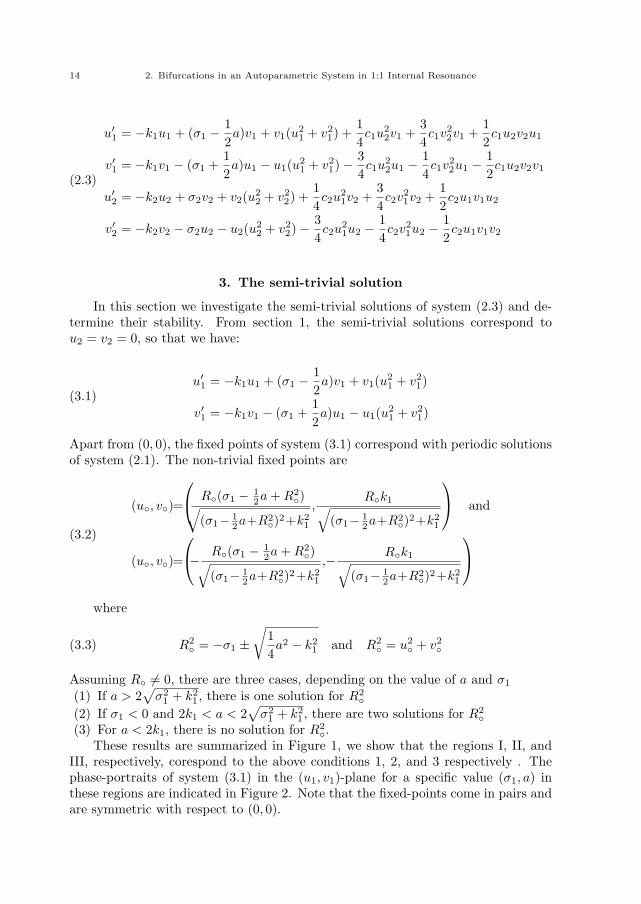
Assuming R◦ 6= 0, there are three cases, depending on the value of a and σ1
(1) If a > 2√
σ21 + k2
1, there is one solution for R2◦
(2) If σ1 < 0 and 2k1 < a < 2√
σ21 + k2
1, there are two solutions for R2◦
(3) For a < 2k1, there is no solution for R2◦.
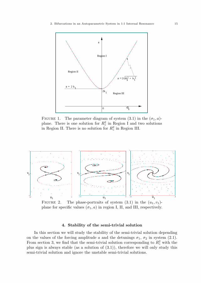
These results are summarized in Figure 1, we show that the regions I, II, andIII, respectively, corespond to the above conditions 1, 2, and 3 respectively . Thephase-portraits of system (3.1) in the (u1, v1)-plane for a specific value (σ1, a) inthese regions are indicated in Figure 2. Note that the fixed-points come in pairs andare symmetric with respect to (0, 0).
2. Bifurcations in an Autoparametric System in 1:1 Internal Resonance 15
a
0
2k1
2 σ12 + k1
2a =
a = 2 k1
σ1
Region III
Region I
Region II
Figure 1. The parameter diagram of system (3.1) in the (σ1, a)-plane. There is one solution for R2
◦ in Region I and two solutionsin Region II. There is no solution for R2
◦ in Region III.
u
v
1
1
u
v
1
1
u
v
1
1
Figure 2. The phase-portraits of system (3.1) in the (u1, v1)-plane for specific values (σ1, a) in region I, II, and III, respectively.
4. Stability of the semi-trivial solution
In this section we will study the stability of the semi-trivial solution dependingon the values of the forcing amplitude a and the detunings σ1, σ2 in system (2.1).From section 3, we find that the semi-trivial solution corresponding to R2
◦ with theplus sign is always stable (as a solution of (3.1)), therefore we will only study thissemi-trivial solution and ignore the unstable semi-trivial solutions.
16 2. Bifurcations in an Autoparametric System in 1:1 Internal Resonance
Write the averaged system (2.3) in the form:
(4.1) X′ = F (X)
where X =
u1
v1
u2
v2
and
(4.2)∂F
∂X=
(A11 A12
A21 A22
)
where A11, A12, A21, and A22 are 2 × 2 matrices depending on u1, v1, u2 and v2.At the solution (±u◦,±v◦, 0, 0), corresponding to the semi-trivial solution of system(4.1), we have ∂F
∂X = AX with(4.3)
A=
0BB@
−k1+2u◦v◦ σ1− 12a+2v2
◦+R2◦ 0 0
−σ1− 12a−2u2
◦−R2◦ −k1−2u◦v◦ 0 0
0 0 −k2+ 12c2u◦v◦ σ2+ 1
4c2u
2◦+
34c2v
2◦
0 0 −σ2− 14c2v
2◦− 3
4c2u
2◦ −k2− 1
2c2u◦v◦
1CCA
u◦ and v◦ satisfy (3.2) and R2◦ satisfies (3.3). Let
A =(
A11 00 A22
)
To get the stability boundary of system (4.1), we solve detA = detA11detA22 = 0.From the equation detA22 = 0, we have:
(4.4) σ2 = −12c2R
2◦ ±
√116
c22R
4◦ − k22 where R2
◦ ≥ 4k2
c2
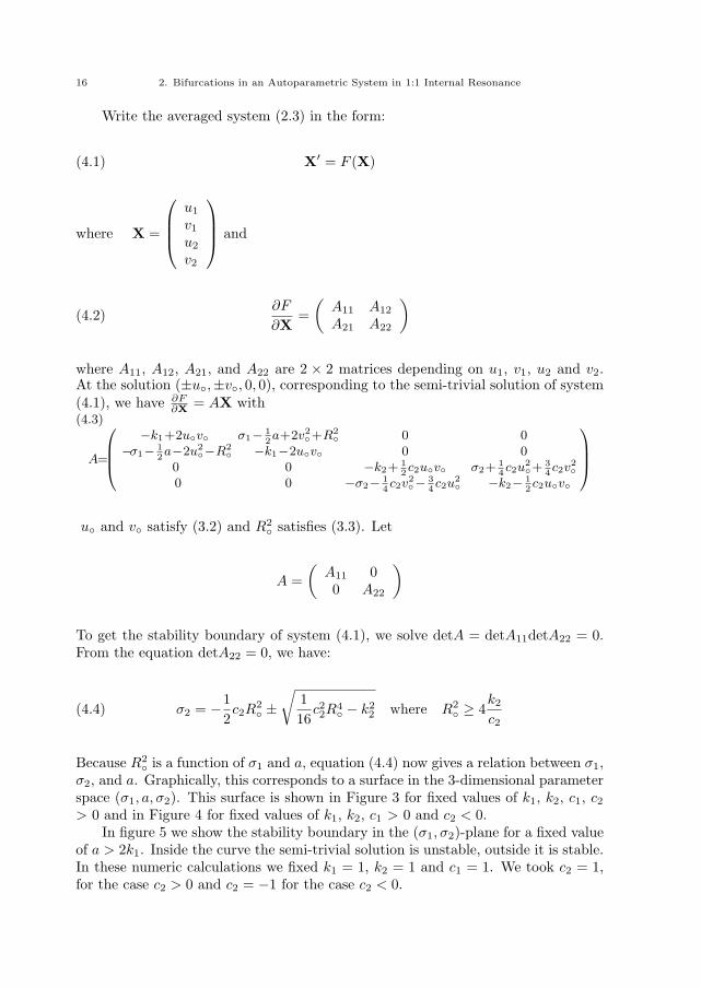
Because R2◦ is a function of σ1 and a, equation (4.4) now gives a relation between σ1,
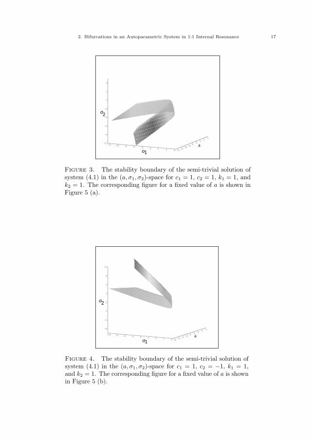
σ2, and a. Graphically, this corresponds to a surface in the 3-dimensional parameterspace (σ1, a, σ2). This surface is shown in Figure 3 for fixed values of k1, k2, c1, c2
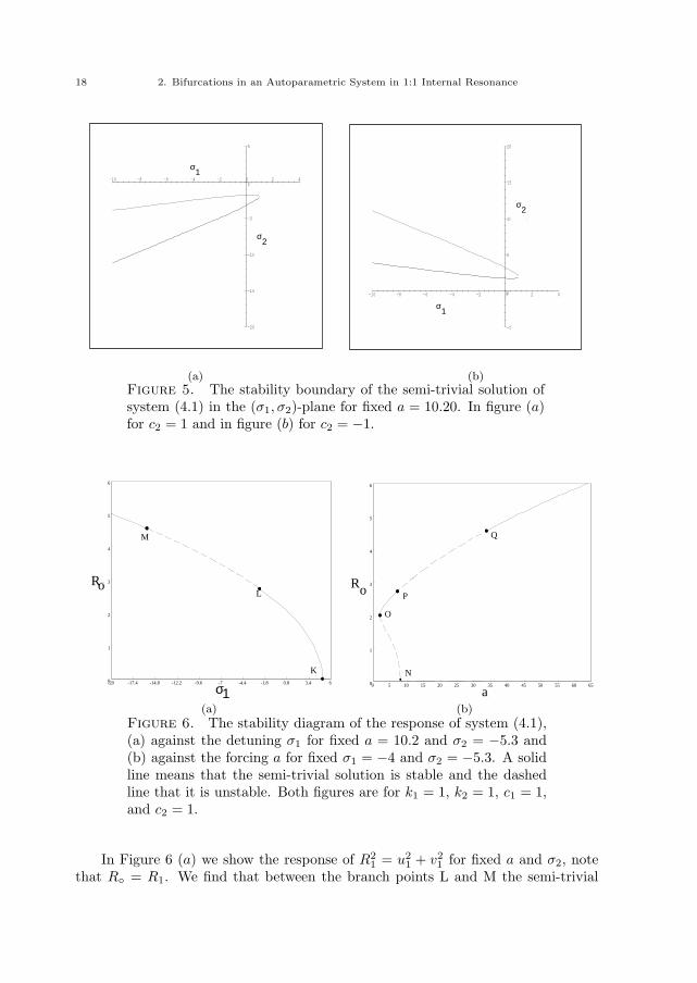
> 0 and in Figure 4 for fixed values of k1, k2, c1 > 0 and c2 < 0.In figure 5 we show the stability boundary in the (σ1, σ2)-plane for a fixed value
of a > 2k1. Inside the curve the semi-trivial solution is unstable, outside it is stable.In these numeric calculations we fixed k1 = 1, k2 = 1 and c1 = 1. We took c2 = 1,for the case c2 > 0 and c2 = −1 for the case c2 < 0.
2. Bifurcations in an Autoparametric System in 1:1 Internal Resonance 17
02
46
810
1214
16
a-12 -10 -8 -6 -4 -2 0 2 4sigma1
-10
-8
-6
-4
-2
0
2
4
σ2
σ1a
Figure 3. The stability boundary of the semi-trivial solution ofsystem (4.1) in the (a, σ1, σ2)-space for c1 = 1, c2 = 1, k1 = 1, andk2 = 1. The corresponding figure for a fixed value of a is shown inFigure 5 (a).
024
68
101214
16a
-12 -10 -8 -6 -4 -2 0 2 4sigma1
-4
-2
0
2
4
6
8
10
σ2
σ1a
Figure 4. The stability boundary of the semi-trivial solution ofsystem (4.1) in the (a, σ1, σ2)-space for c1 = 1, c2 = −1, k1 = 1,and k2 = 1. The corresponding figure for a fixed value of a is shownin Figure 5 (b).
18 2. Bifurcations in an Autoparametric System in 1:1 Internal Resonance
-20
-15
-10
-5
0
5
sigma2
-10 -8 -6 -4 -2 0 2 4sigma1
σ2
σ1
-5
0
5
10
15
20
sigma2
-10 -8 -6 -4 -2 0 2 4sigma1
σ2
σ1
(a) (b)Figure 5. The stability boundary of the semi-trivial solution ofsystem (4.1) in the (σ1, σ2)-plane for fixed a = 10.20. In figure (a)for c2 = 1 and in figure (b) for c2 = −1.
0
1
2
3
4
5
6
-20 -17.4 -14.8 -12.2 -9.6 -7 -4.4 -1.8 0.8 3.4 6sigma1
L2_NormRo
K
L
M
σ10
1
2
3
4
5
6
0 5 10 15 20 25 30 35 40 45 50 55 60 65a
L2_NormRo
N
O
P
Q
.a
(a) (b)
Figure 6. The stability diagram of the response of system (4.1),(a) against the detuning σ1 for fixed a = 10.2 and σ2 = −5.3 and(b) against the forcing a for fixed σ1 = −4 and σ2 = −5.3. A solidline means that the semi-trivial solution is stable and the dashedline that it is unstable. Both figures are for k1 = 1, k2 = 1, c1 = 1,and c2 = 1.
In Figure 6 (a) we show the response of R21 = u2
1 + v21 for fixed a and σ2, note
that R◦ = R1. We find that between the branch points L and M the semi-trivial
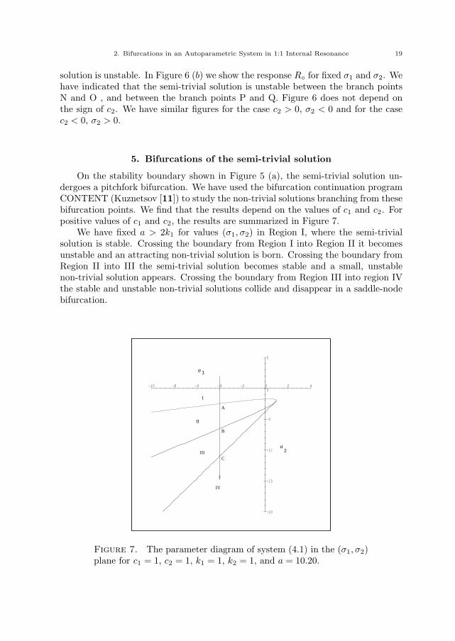
2. Bifurcations in an Autoparametric System in 1:1 Internal Resonance 19
solution is unstable. In Figure 6 (b) we show the response R◦ for fixed σ1 and σ2. Wehave indicated that the semi-trivial solution is unstable between the branch pointsN and O , and between the branch points P and Q. Figure 6 does not depend onthe sign of c2. We have similar figures for the case c2 > 0, σ2 < 0 and for the casec2 < 0, σ2 > 0.
5. Bifurcations of the semi-trivial solution
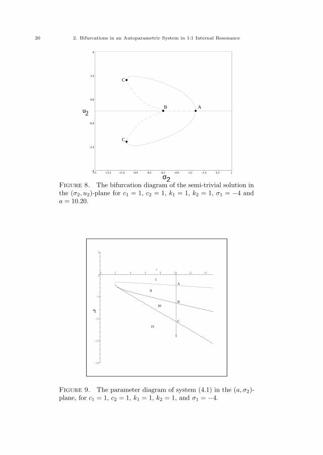
On the stability boundary shown in Figure 5 (a), the semi-trivial solution un-dergoes a pitchfork bifurcation. We have used the bifurcation continuation programCONTENT (Kuznetsov [11]) to study the non-trivial solutions branching from thesebifurcation points. We find that the results depend on the values of c1 and c2. Forpositive values of c1 and c2, the results are summarized in Figure 7.
We have fixed a > 2k1 for values (σ1, σ2) in Region I, where the semi-trivialsolution is stable. Crossing the boundary from Region I into Region II it becomesunstable and an attracting non-trivial solution is born. Crossing the boundary fromRegion II into III the semi-trivial solution becomes stable and a small, unstablenon-trivial solution appears. Crossing the boundary from Region III into region IVthe stable and unstable non-trivial solutions collide and disappear in a saddle-nodebifurcation.
-20
-15
-10
-5
0
5
sigma2
-10 -8 -6 -4 -2 0 2 4sigma1
I
II
III
IV
A
B
C
σ2
σ 1
Figure 7. The parameter diagram of system (4.1) in the (σ1, σ2)plane for c1 = 1, c2 = 1, k1 = 1, k2 = 1, and a = 10.20.
20 2. Bifurcations in an Autoparametric System in 1:1 Internal Resonance
-4
-2.4
-0.8
0.8
2.4
4
-15 -13.3 -11.6 -9.9 -8.2 -6.5 -4.8 -3.1 -1.4 0.3 2sigma2
u2
σ2
u2AB
C
C
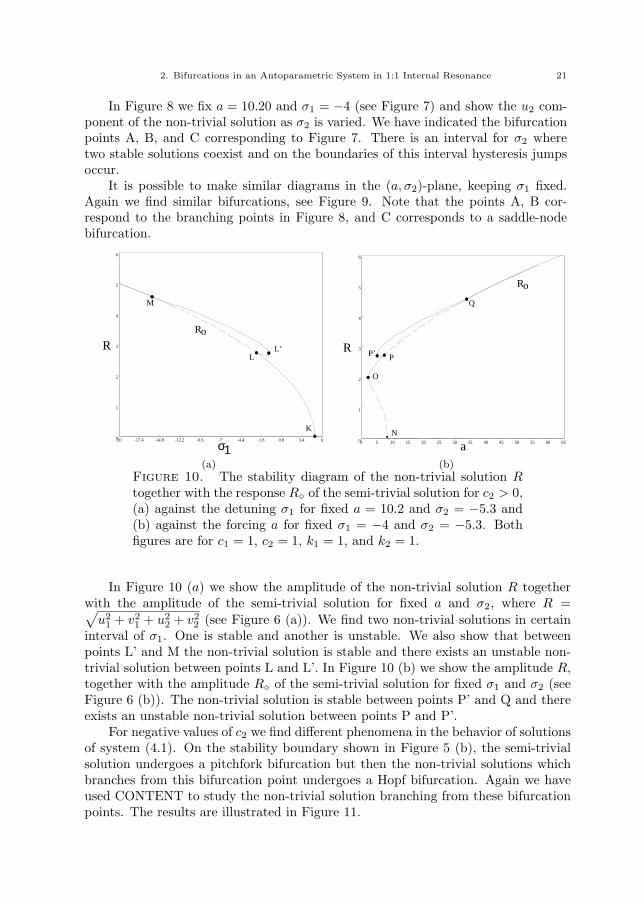
Figure 8. The bifurcation diagram of the semi-trivial solution inthe (σ2, u2)-plane for c1 = 1, c2 = 1, k1 = 1, k2 = 1, σ1 = −4 anda = 10.20.
-20
-15
-10
-5
0
5
sigma2
0 2 4 6 8 10 12 14a
σ2
A
B
C
I
II
III
IV
Figure 9. The parameter diagram of system (4.1) in the (a, σ2)-plane, for c1 = 1, c2 = 1, k1 = 1, k2 = 1, and σ1 = −4.
2. Bifurcations in an Autoparametric System in 1:1 Internal Resonance 21
In Figure 8 we fix a = 10.20 and σ1 = −4 (see Figure 7) and show the u2 com-ponent of the non-trivial solution as σ2 is varied. We have indicated the bifurcationpoints A, B, and C corresponding to Figure 7. There is an interval for σ2 wheretwo stable solutions coexist and on the boundaries of this interval hysteresis jumpsoccur.
It is possible to make similar diagrams in the (a, σ2)-plane, keeping σ1 fixed.Again we find similar bifurcations, see Figure 9. Note that the points A, B cor-respond to the branching points in Figure 8, and C corresponds to a saddle-nodebifurcation.
0
1
2
3
4
5
6
-20 -17.4 -14.8 -12.2 -9.6 -7 -4.4 -1.8 0.8 3.4 6sigma1
L2_Norm
K
L
M
L’
Ro
R
σ10
1
2
3
4
5
6
0 5 10 15 20 25 30 35 40 45 50 55 60 65a
L2_NormR
a
Ro
N
O
P
Q
P’
.
(a) (b)Figure 10. The stability diagram of the non-trivial solution Rtogether with the response R◦ of the semi-trivial solution for c2 > 0,(a) against the detuning σ1 for fixed a = 10.2 and σ2 = −5.3 and(b) against the forcing a for fixed σ1 = −4 and σ2 = −5.3. Bothfigures are for c1 = 1, c2 = 1, k1 = 1, and k2 = 1.
In Figure 10 (a) we show the amplitude of the non-trivial solution R togetherwith the amplitude of the semi-trivial solution for fixed a and σ2, where R =√
u21 + v2
1 + u22 + v2
2 (see Figure 6 (a)). We find two non-trivial solutions in certaininterval of σ1. One is stable and another is unstable. We also show that betweenpoints L’ and M the non-trivial solution is stable and there exists an unstable non-trivial solution between points L and L’. In Figure 10 (b) we show the amplitude R,together with the amplitude R◦ of the semi-trivial solution for fixed σ1 and σ2 (seeFigure 6 (b)). The non-trivial solution is stable between points P’ and Q and thereexists an unstable non-trivial solution between points P and P’.
For negative values of c2 we find different phenomena in the behavior of solutionsof system (4.1). On the stability boundary shown in Figure 5 (b), the semi-trivialsolution undergoes a pitchfork bifurcation but then the non-trivial solutions whichbranches from this bifurcation point undergoes a Hopf bifurcation. Again we haveused CONTENT to study the non-trivial solution branching from these bifurcationpoints. The results are illustrated in Figure 11.
22 2. Bifurcations in an Autoparametric System in 1:1 Internal Resonance
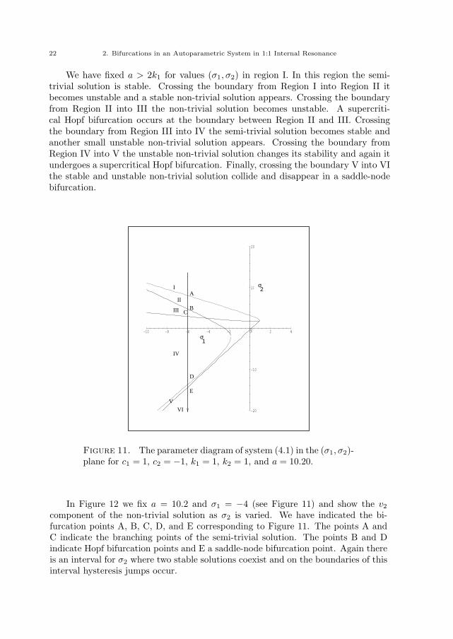
We have fixed a > 2k1 for values (σ1, σ2) in region I. In this region the semi-trivial solution is stable. Crossing the boundary from Region I into Region II itbecomes unstable and a stable non-trivial solution appears. Crossing the boundaryfrom Region II into III the non-trivial solution becomes unstable. A supercriti-cal Hopf bifurcation occurs at the boundary between Region II and III. Crossingthe boundary from Region III into IV the semi-trivial solution becomes stable andanother small unstable non-trivial solution appears. Crossing the boundary fromRegion IV into V the unstable non-trivial solution changes its stability and again itundergoes a supercritical Hopf bifurcation. Finally, crossing the boundary V into VIthe stable and unstable non-trivial solution collide and disappear in a saddle-nodebifurcation.
-20
-10
0
10
20
sigma2
-10 -8 -6 -4 -2 0 2 4sigma1
A
BC
D
E
I
II
III
IV
VVI
σ2
σ1
VI
Figure 11. The parameter diagram of system (4.1) in the (σ1, σ2)-plane for c1 = 1, c2 = −1, k1 = 1, k2 = 1, and a = 10.20.
In Figure 12 we fix a = 10.2 and σ1 = −4 (see Figure 11) and show the v2
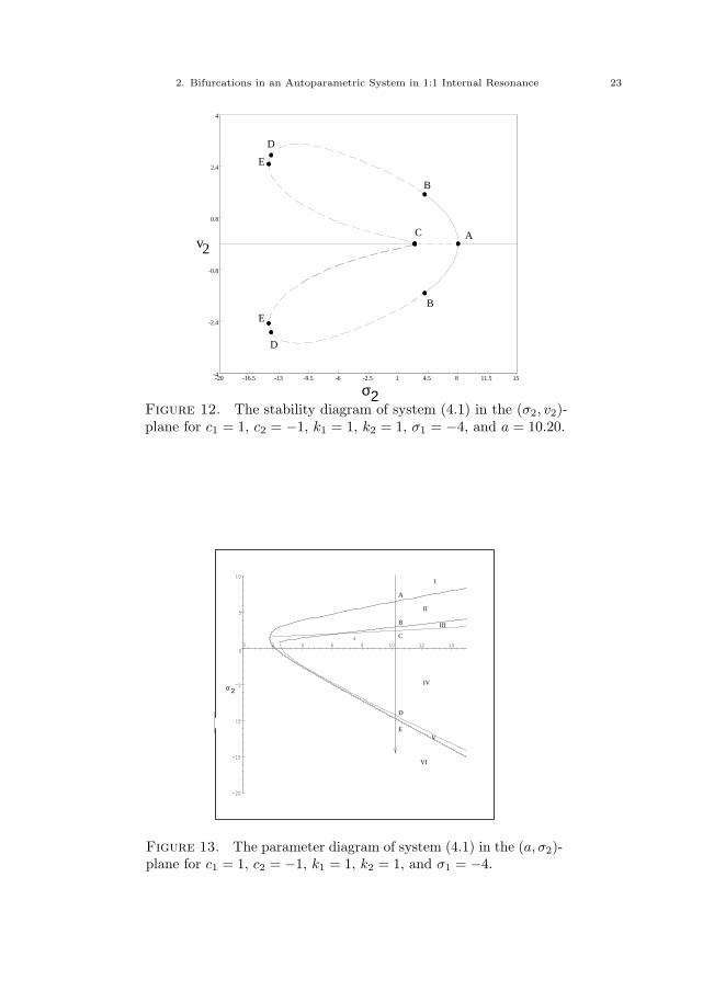
component of the non-trivial solution as σ2 is varied. We have indicated the bi-furcation points A, B, C, D, and E corresponding to Figure 11. The points A andC indicate the branching points of the semi-trivial solution. The points B and Dindicate Hopf bifurcation points and E a saddle-node bifurcation point. Again thereis an interval for σ2 where two stable solutions coexist and on the boundaries of thisinterval hysteresis jumps occur.
2. Bifurcations in an Autoparametric System in 1:1 Internal Resonance 23
-4
-2.4
-0.8
0.8
2.4
4
-20 -16.5 -13 -9.5 -6 -2.5 1 4.5 8 11.5 15sigma2
v2
A
B
B
C
D
D
E
E
σ2
v2
Figure 12. The stability diagram of system (4.1) in the (σ2, v2)-plane for c1 = 1, c2 = −1, k1 = 1, k2 = 1, σ1 = −4, and a = 10.20.
-20
-15
-10
-5
0
5
10
sigma2
0 2 4 6 8 10 12 14a
σ 2
A
B
C
D
E
I
II
III
IV
V
VI
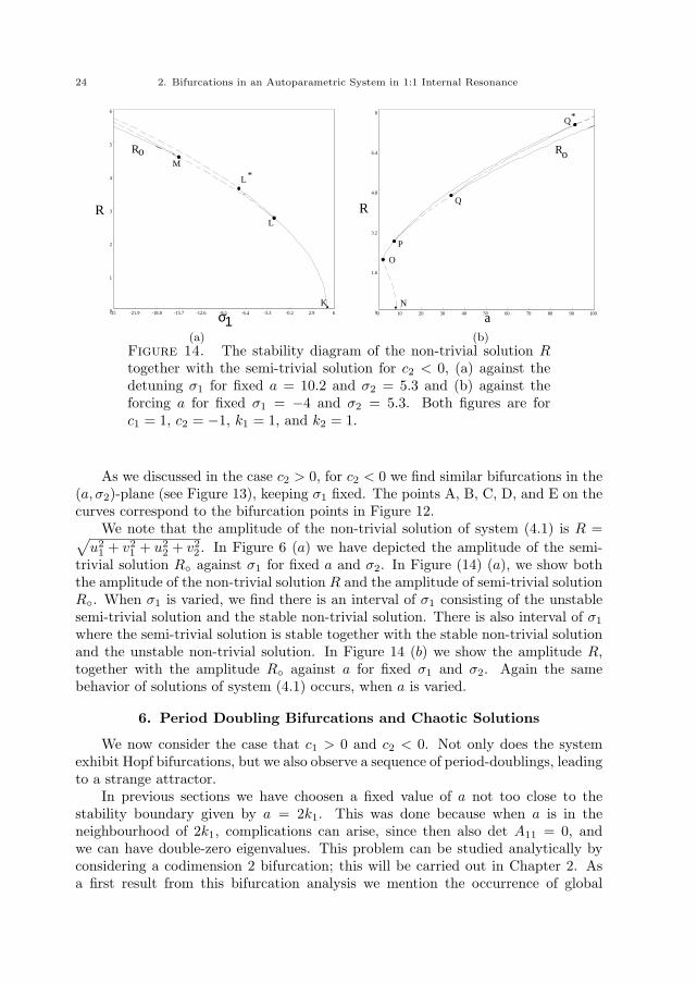
Figure 13. The parameter diagram of system (4.1) in the (a, σ2)-plane for c1 = 1, c2 = −1, k1 = 1, k2 = 1, and σ1 = −4.
24 2. Bifurcations in an Autoparametric System in 1:1 Internal Resonance
0
1
2
3
4
5
6
-25 -21.9 -18.8 -15.7 -12.6 -9.5 -6.4 -3.3 -0.2 2.9 6sigma1
L2_Norm
.
R
K
L
M
Ro
L *
σ10
1.6
3.2
4.8
6.4
8
0 10 20 30 40 50 60 70 80 90 100a
L2_Norm
.a
Ro
N
O
P
Q
Q*
R
(a) (b)Figure 14. The stability diagram of the non-trivial solution Rtogether with the semi-trivial solution for c2 < 0, (a) against thedetuning σ1 for fixed a = 10.2 and σ2 = 5.3 and (b) against theforcing a for fixed σ1 = −4 and σ2 = 5.3. Both figures are forc1 = 1, c2 = −1, k1 = 1, and k2 = 1.
As we discussed in the case c2 > 0, for c2 < 0 we find similar bifurcations in the(a, σ2)-plane (see Figure 13), keeping σ1 fixed. The points A, B, C, D, and E on thecurves correspond to the bifurcation points in Figure 12.
We note that the amplitude of the non-trivial solution of system (4.1) is R =√u2
1 + v21 + u2
2 + v22 . In Figure 6 (a) we have depicted the amplitude of the semi-
trivial solution R◦ against σ1 for fixed a and σ2. In Figure (14) (a), we show boththe amplitude of the non-trivial solution R and the amplitude of semi-trivial solutionR◦. When σ1 is varied, we find there is an interval of σ1 consisting of the unstablesemi-trivial solution and the stable non-trivial solution. There is also interval of σ1
where the semi-trivial solution is stable together with the stable non-trivial solutionand the unstable non-trivial solution. In Figure 14 (b) we show the amplitude R,together with the amplitude R◦ against a for fixed σ1 and σ2. Again the samebehavior of solutions of system (4.1) occurs, when a is varied.
6. Period Doubling Bifurcations and Chaotic Solutions
We now consider the case that c1 > 0 and c2 < 0. Not only does the systemexhibit Hopf bifurcations, but we also observe a sequence of period-doublings, leadingto a strange attractor.
In previous sections we have choosen a fixed value of a not too close to thestability boundary given by a = 2k1. This was done because when a is in theneighbourhood of 2k1, complications can arise, since then also det A11 = 0, andwe can have double-zero eigenvalues. This problem can be studied analytically byconsidering a codimension 2 bifurcation; this will be carried out in Chapter 2. Asa first result from this bifurcation analysis we mention the occurrence of global
2. Bifurcations in an Autoparametric System in 1:1 Internal Resonance 25
bifurcations, involving heteroclinic and homoclinic loops. We also find a homoclinicsolution of Silnikov type. It is well-known (see Kuznetsov [11] and Wiggins [12])that the existence of such a homoclinic loop is connected with chaotic solutions. Wetherefore conjecture that the chaotic solutions we find numerically are the result ofthe Silnikov phenomenon.
A
B
C
D
E
I
σ2
II
III
IV
V
VI
Figure 15. The parameter diagram of system (4.1) in the (a, σ2)-plane for c2 < 0 close to the stability boundary.
In the numeric calculations, presented in this section interesting behavior ofsolutions of system (4.1) occurs near the stability boundary.
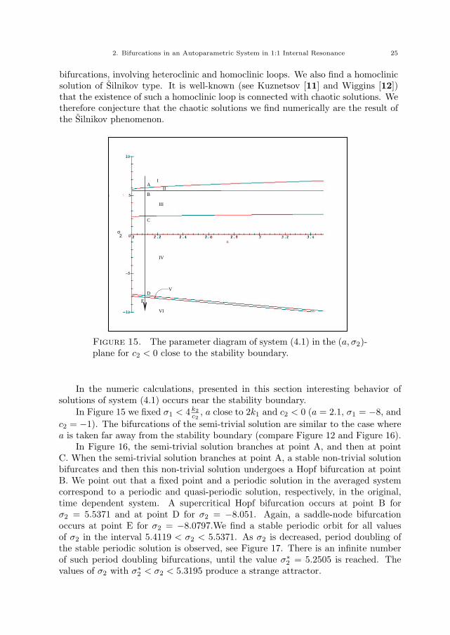
In Figure 15 we fixed σ1 < 4k2c2
, a close to 2k1 and c2 < 0 (a = 2.1, σ1 = −8, andc2 = −1). The bifurcations of the semi-trivial solution are similar to the case wherea is taken far away from the stability boundary (compare Figure 12 and Figure 16).
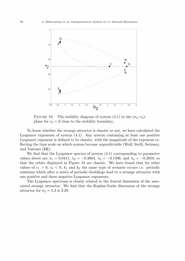
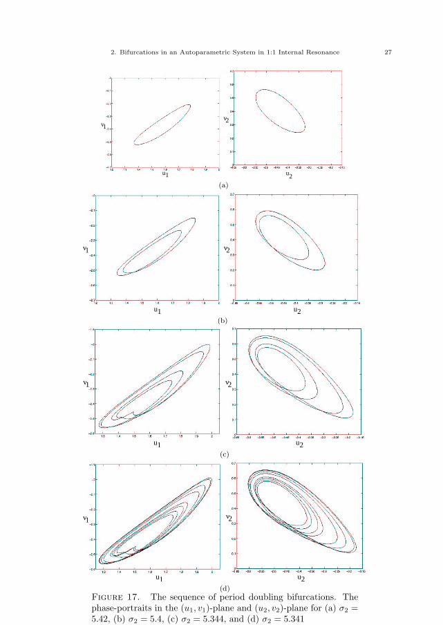
In Figure 16, the semi-trivial solution branches at point A, and then at pointC. When the semi-trivial solution branches at point A, a stable non-trivial solutionbifurcates and then this non-trivial solution undergoes a Hopf bifurcation at pointB. We point out that a fixed point and a periodic solution in the averaged systemcorrespond to a periodic and quasi-periodic solution, respectively, in the original,time dependent system. A supercritical Hopf bifurcation occurs at point B forσ2 = 5.5371 and at point D for σ2 = −8.051. Again, a saddle-node bifurcationoccurs at point E for σ2 = −8.0797.We find a stable periodic orbit for all valuesof σ2 in the interval 5.4119 < σ2 < 5.5371. As σ2 is decreased, period doubling ofthe stable periodic solution is observed, see Figure 17. There is an infinite numberof such period doubling bifurcations, until the value σ∗2 = 5.2505 is reached. Thevalues of σ2 with σ∗2 < σ2 < 5.3195 produce a strange attractor.
26 2. Bifurcations in an Autoparametric System in 1:1 Internal Resonance
-4
-2.4
-0.8
0.8
2.4
4
-10 -8.5 -7 -5.5 -4 -2.5 -1 0.5 2 3.5 5 6.5 8sigma2
v2
σ2
v2A
B
B
C
D
E
ED
Figure 16. The stability diagram of system (4.1) in the (σ2, v2)-plane for c2 < 0 close to the stability boundary.
To know whether the strange attractor is chaotic or not, we have calculated theLyapunov exponents of system (4.1). Any system containing at least one positiveLyapunov exponent is defined to be chaotic, with the magnitude of the exponent re-flecting the time scale on which system become unpredictable (Wolf, Swift, Swinney,and Vastano [13]).
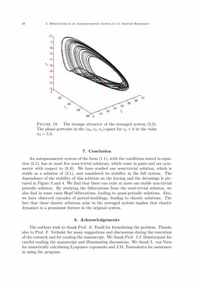
We find that the Lyapunov spectra of system (4.1) corresponding to parametervalues above are λ1 = 0.8411, λ2 = −0.3864, λ3 = −0.1596, and λ4 = −0.2858, sothat the orbits displayed in Figure 18 are chaotic. We have found that for othervalues of c1 > 0, c2 < 0, k1 and k2 the same type of scenario occurs i.e. periodicsolutions which after a series of periodic-doublings lead to a strange attractor withone positive and three negative Lyapunov exponents.
The Lyapunov spectrum is closely related to the fractal dimension of the asso-ciated strange attractor. We find that the Kaplan-Yorke dimension of the strangeattractor for σ2 = 5.3 is 2.29.
2. Bifurcations in an Autoparametric System in 1:1 Internal Resonance 27
u1
v1
u2
v2
(a)
u1
v1
u2
v2
(b)
u1
v1
u2
v2
(c)
u1
v1
u2
v2
(d)Figure 17. The sequence of period doubling bifurcations. Thephase-portraits in the (u1, v1)-plane and (u2, v2)-plane for (a) σ2 =5.42, (b) σ2 = 5.4, (c) σ2 = 5.344, and (d) σ2 = 5.341
28 2. Bifurcations in an Autoparametric System in 1:1 Internal Resonance
v2
u2
u1
Figure 18. The strange attractor of the averaged system (2.3).The phase-portraits in the (u2, v2, u1)-space for c2 < 0 at the valueσ2 = 5.3.
7. Conclusion
An autoparametric system of the form (1.1), with the conditions stated in equa-tion (2.1), has at most five semi-trivial solutions, which come in pairs and are sym-metric with respect to (0, 0). We have studied one semi-trivial solution, which isstable as a solution of (3.1), and considered its stability in the full system. Thedependence of the stability of this solution on the forcing and the detunings is pic-tured in Figure 3 and 4. We find that there can exist at most one stable non-trivialperiodic solution. By studying the bifurcations from the semi-trivial solution, wealso find in some cases Hopf bifurcations, leading to quasi-periodic solutions. Also,we have observed cascades of period-doublings, leading to chaotic solutions. Thefact that these chaotic solutions arise in the averaged system implies that chaoticdynamics is a prominent feature in the original system.
8. Acknowledgements
The authors wish to thank Prof. A. Tondl for formulating the problem. Thanksalso to Prof. F. Verhulst for many suggestions and discussions during the executionof the research and for reading the manuscript. We thank Prof. J.J. Duistermaat forcareful reading the manuscript and illuminating discussions. We thank L. van Veenfor numerically calculating Lyapunov exponents and J.M. Tuwankotta for assistancein using the program.

2. Bifurcations in an Autoparametric System in 1:1 Internal Resonance 29
The research was conducted in the department of Mathematics of the Universityof Utrecht and supported by project of PGSM from Indonesia and CICAT TU Delft.

Bibliography
[1] R. Svoboda, A. Tondl, and F. Verhulst, Autoparametric Resonance by Coupling of Linear andNonlinear Systems, J. Non-linear Mechanics. 29 (1994) 225-232.
[2] A. Tondl, M. Ruijgrok, F. Verhulst, and R. Nabergoj, Autoparametric Resonance in Mechan-ical Systems, Cambridge University Press, New York, 2000.
[3] M. Ruijgrok, Studies in Parametric and Autoparametric Resonance, Ph.D. Thesis, UniversiteitUtrecht, 1995.
[4] S.S. Oueini, C. Chin, and A.H. Nayfeh, Response of Two Quadratically Coupled Oscillatorsto a Principal Parametric Excitation, to Appear J. of Vibration and Control.
[5] W. Tien, N.S Namachchivaya, and A.K. Bajaj, Non-Linear Dynamics of a Shallow Arch underPeriodic Excitation-I. 1:2 Internal Resonance, Int. J. Non-Linear Mechanics, 29 (1994) 349-366.
[6] A.K. Bajaj, S.I. Chang, and J.M Johnson, Amplitude Modulated Dynamics of a ResonantlyExcited Autoparametric Two Degree-of-Freedom System, Nonlinear Dynamics, 5 (1994) 433-457.
[7] B. Banerjee, and A.K. Bajaj, Amplitude Modulated Chaos in Two Degree-of-Fredoom Systemswith Quadratic Nonlinearities, Acta Mechanica, 124 (1997) 131-154.
[8] W. Tien, N.S. Namachchivaya, and N. Malhotra, Non-Linear Dynamics of a Shallow Archunder Periodic Excitation-II. 1:1 Internal Resonance, Int. J. Non-Linear Mechanics, 29 (1994)367-386.
[9] Z. Feng, and P. Sethna, Global Bifurcation and Chaos in Parametrically Forced Systems withone-one Resonance, Dyn.Stability Syst., 5 (1990) 201-225.
[10] J.A. Sanders, and F. Verhulst, Averaging Methods in Nonlinear Dynamical System,Appl.math. Sciences 59, Springer-Verlag, New York, 1985.
[11] Y. Kuznetsov and V. Levitin, CONTENT: Integrated Environment for the Analysis of Dy-namical Systems, Centrum voor Wiskunde en Informatica, Amsterdam, The Netherlands,ftp://ftp.cwi.nl/pub/CONTENT, 1997.
[12] S. Wiggins, Global Bifurcation and Chaos, Applied Mathematical Science 73, Springer-Verlag,New York, 1988.
[13] A. Wolf, J.B. Swift, H.L. Swinney, and J.A. Vastano, Determining Lyapunov Exponent froma Time Series, Physica. 16D (1985) 285-317.
31