Embed Size (px)
Citation preview
8888 Big Data: Baseline Forecasting With Exponential Smoothing Models
Exponential smoothing models provide a viable framework for forecasting large volume, disaggregate
demand patterns. For short-term planning and control systems, these techniques are extremely reliable
and have more than adequate track record in forecast accuracy with trend/seasonal data.
This chapter deals with the description and evaluation of techniques that
• are widely used in the areas of sales, inventory, logistics, and production planning as well as in
quality control, process control, financial planning and marketing planning
• can be described in terms of a state-space modeling framework that provides prediction intervals
and procedures for model selection are well-suited for large-scale, automated forecasting
applications, because they require little forecaster intervention, thereby releasing the time of the
demand forecaster to concentrate on the few problem cases
• are based on the mathematical extrapolation of past patterns into the future, accomplished by
using forecasting equations that are simple to update and require relatively small number of
calculations
• capture level (a starting point for the forecasts), trend (a factor for growth or decline) and seasonal
factors (for adjustment of seasonal variation) in data patterns
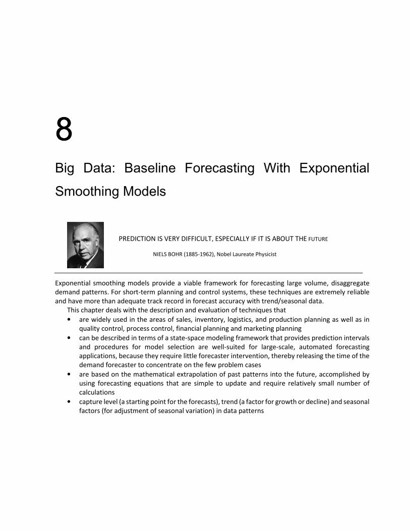
PREDICTION IS VERY DIFFICULT, ESPECIALLY IF IT IS ABOUT THE FUTURE
NIELS BOHR (1885-1962), Nobel Laureate Physicist

What is Exponential Smoothing?
In chapter 3, we introduced forecasting with simple and weighted moving averages as an exploratory
smoothing technique for short-term forecasting of level data. With exponential smoothing models, on the
other hand, we can create short-term forecasts with prediction limits for a wider variety of data having
trends and seasonal patterns; the modeling methodology offers prediction limits (ranges of uncertainty)
and prescribed forecast profiles. Exponential smoothing provides an essential simplicity and ease of
understanding for the practitioner, and has been found to have a reliable track record for accuracy in
many business applications.
Exponential smoothing was invented during World War II by Robert G. Brown
(1923 ̶2013), left, who was involved in the design of tracking systems for fire-control
information on the location of enemy submarines. Later on, the principles of
exponential smoothing were applied to business data, especially in the analysis of the
demand for service parts in inventory systems in Brown’s book Advanced Service Parts
Inventory Control (1982).
As part of the state-space forecasting methodology, exponential smoothing
models provide a flexible approach to weighting past historical data for smoothing and
extrapolation purposes. This exponentially declining weighting scheme contrasts with the equal weighting
scheme that underlies the outmoded simple moving average technique for forecasting.
Exponential smoothing is a forecasting technique that extrapolates historical patterns such as
trends and seasonal cycles into the future.
There are many types of exponential smoothing models, each appropriate for a
particular forecast pattern or forecast profile. As a forecasting tool, exponential
smoothing is very widely accepted and a proven tool for a wide variety of short-term
forecasting applications. Most inventory planning and production control systems
rely on exponential smoothing to some degree.
We will see that the process for assigning smoothing weights is simple in concept
and versatile for dealing with diverse types of data. Other advantages of exponential smoothing are that
the methodology takes account of trend and seasonal patterns in time series; embodies a weighting
scheme that gives more weight to the recent past than to the distant past; is readily automated, making
it especially useful for large-scale forecasting applications; and can be described in a modeling framework
needed for deriving useful statistical prediction limits and flexible trend/seasonal forecast profiles.
When selecting a model for demand forecasting, focus on plausible forecast profiles, rather
than fit statistics and model coefficients.
For demand forecasting, the disadvantages are that exponential smoothing models do not easily
allow for the inclusion of explanatory variables into a forecasting model and cannot handle business
cycles. Hence, when forecasting economic variables, such techniques are not expected to perform well on
business data that exhibit cyclical turning points.
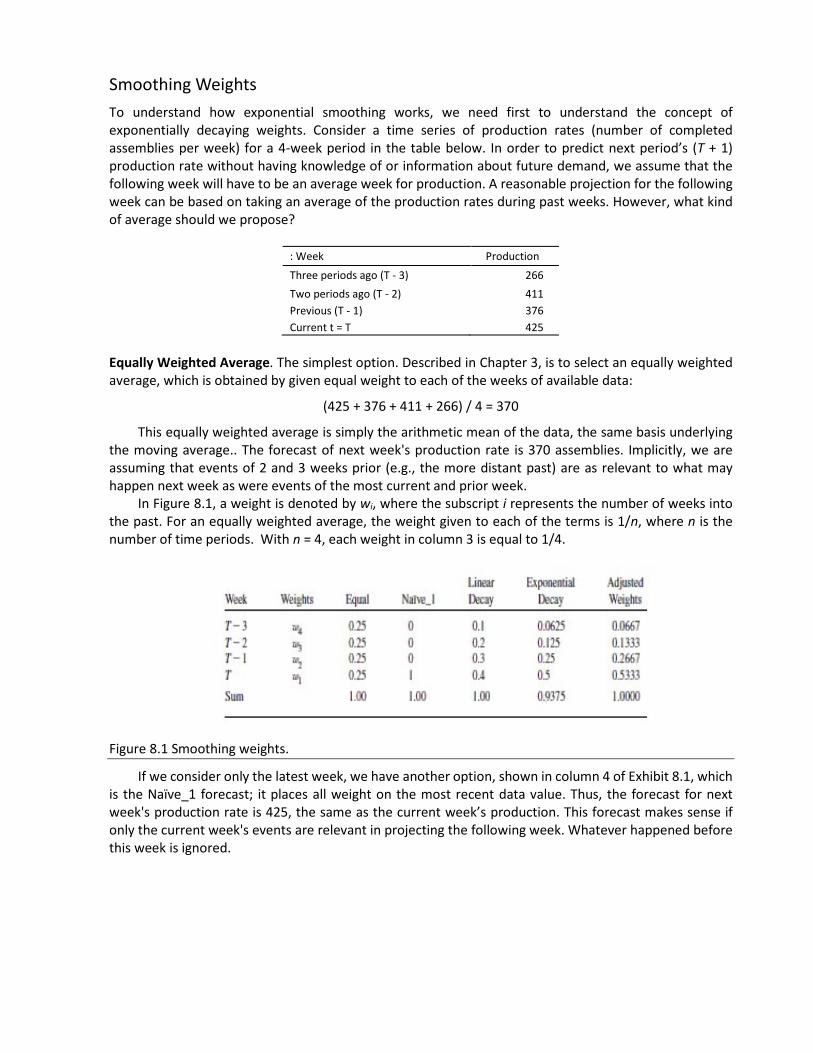
Smoothing Weights
To understand how exponential smoothing works, we need first to understand the concept of
exponentially decaying weights. Consider a time series of production rates (number of completed
assemblies per week) for a 4-week period in the table below. In order to predict next period’s (T + 1)
production rate without having knowledge of or information about future demand, we assume that the
following week will have to be an average week for production. A reasonable projection for the following
week can be based on taking an average of the production rates during past weeks. However, what kind
of average should we propose?
: Week Production
Three periods ago (T - 3) 266
Two periods ago (T - 2) 411
Previous (T - 1) 376
Current t = T 425
Equally Weighted Average. The simplest option. Described in Chapter 3, is to select an equally weighted
average, which is obtained by given equal weight to each of the weeks of available data:
(425 + 376 + 411 + 266) / 4 = 370
This equally weighted average is simply the arithmetic mean of the data, the same basis underlying
the moving average.. The forecast of next week's production rate is 370 assemblies. Implicitly, we are
assuming that events of 2 and 3 weeks prior (e.g., the more distant past) are as relevant to what may
happen next week as were events of the most current and prior week.
In Figure 8.1, a weight is denoted by wi, where the subscript i represents the number of weeks into
the past. For an equally weighted average, the weight given to each of the terms is 1/n, where n is the
number of time periods. With n = 4, each weight in column 3 is equal to 1/4.
Figure 8.1 Smoothing weights.
If we consider only the latest week, we have another option, shown in column 4 of Exhibit 8.1, which
is the Naïve_1 forecast; it places all weight on the most recent data value. Thus, the forecast for next
week's production rate is 425, the same as the current week’s production. This forecast makes sense if
only the current week's events are relevant in projecting the following week. Whatever happened before
this week is ignored.
Exponentially Decaying Weights. Most business forecasters find a middle ground more appealing than
either of the two extremes, equally weighted or Naïve_1. In between lie weighting schemes in which the
weights decay as we move from the current period to the distant past.
w1 > w2 > w3 > w4 >. . . .
The largest weight, w1, is given to the most recent data value. This means that to forecast next week's
production rate, this week's figure is most important; last week's is less important, and so forth.
Many other patterns are possible with decaying weight schemes. As illustrated by column 5 of Figure
8.1, the weight starts at 40% for the most recent week and decline steadily to 10% for week T - 3. Our
forecast for week t = T + 1 is the weighted average with decaying weights:
425 x 0.4 + 376 x 0.3 + 411 x 0.2 + 266 x 0.1 = 392
This weighted average gives a production rate forecast that is more than that of the equally weighted
average and less than that of the Naïve_1, in this case.
An exponentially weighted average refers to a weighted average of the data in which the weights decay
exponentially.
The most useful example of decaying weights is that of exponentially decaying weights, in which each
weight is a constant fraction of its predecessor. A fraction of 0.50 implies a decay rate of 50%, as shown
in column 6 of Figure 8.1. In forecasting next period’s value, the current period’s value is weighted 0.5,
the prior week half of that at 0.25, and so forth with each new weight 50% of the one before. (These
weights must be adjusted to sum to unity as in column 7.) From Figure 8.1, we can see that the adjusted
weights are obtained by dividing the exponential decay weights by 0.9375.
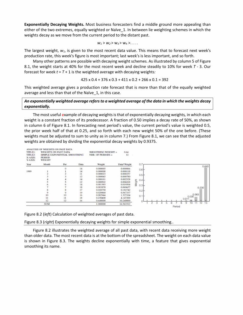
Figure 8.2 (left) Calculation of weighted averages of past data.
Figure 8.3 (right) Exponentially decaying weights for simple exponential smoothing..
Figure 8.2 illustrates the weighted average of all past data, with recent data receiving more weight
than older data. The most recent data is at the bottom of the spreadsheet. The weight on each data value
is shown in Figure 8.3. The weights decline exponentially with time, a feature that gives exponential
smoothing its name.
The Simple Exponential Smoothing Method
All exponential smoothing techniques incorporate an exponential-decay weighting system, hence the
term exponential. Smoothing refers to the averaging that takes place when we calculate a weighted
average of the past data. To determine a one-period-ahead forecast of historical data, the projection
formula is given by
Yt (1) = α Yt + (1 - α) Yt-1 (1)
where Yt (1) is the smoothed value at time t, based on weighting the most recent value Yt with a weight α
(α is a smoothing parameter) and the current period’s forecast (or previous smoothed value) with a weight
(1 - α). By rearranging the right-hand side, we can rewrite the equation as
Yt (1) = Yt-1 (1) + α [Yt - Yt-1 (1)]
which can be interpreted as the current period’s forecast Yt-1 (1) adjusted by a proportion α of the current
period’s forecast error [Yt - Yt-1 (1)].
The simple exponential smoothing method produces forecasts that are a level line for any
period in the future, but it is not appropriate for projecting trending data or patterns that are
more complex.
We can now show that the one-step-ahead forecast Yt (1) is a weighted moving average
of all past values with the weights decreasing exponentially. If we substitute for Yt-1 (1) in
the first smoothing equation, we find that:
Yt (1) = α Yt + (1 - α) [α Yt-1 + (1 - α) Yt - 2 (1)]
= α Yt + α (1 - α) Yt-1 + (1 - α)2 Yt - 2 (1)
If we next substitute for Y t-2 (1), then for Y t-3 (1), and so, we obtain the result
Yt (1) = α Yt + α (1 - α) Yt-1 + α (1 - α)2 Yt - 2 + α (1 - α)3 Yt – 3 + α (1 - α)4 Yt - 4
+ . . . . + α (1 - α)t- 1 Y1 + (1 - α)t Y0 (1)
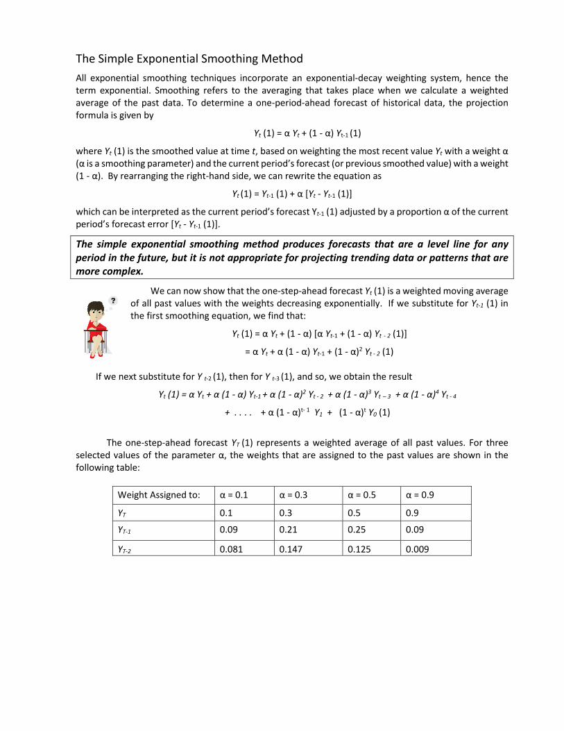
The one-step-ahead forecast YT (1) represents a weighted average of all past values. For three
selected values of the parameter α, the weights that are assigned to the past values are shown in the
following table:
Weight Assigned to: α = 0.1 α = 0.3 α = 0.5 α = 0.9
YT 0.1 0.3 0.5 0.9
YT-1 0.09 0.21 0.25 0.09
YT-2 0.081 0.147 0.125 0.009
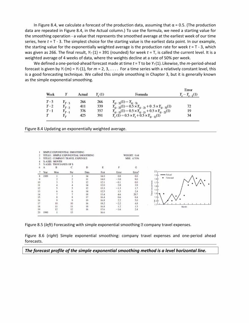
In Figure 8.4, we calculate a forecast of the production data, assuming that α = 0.5. (The production
data are repeated in Figure 8.4, in the Actual column.) To use the formula, we need a starting value for
the smoothing operation - a value that represents the smoothed average at the earliest week of our time
series, here t = T - 3. The simplest choice for the starting value is the earliest data point. In our example,
the starting value for the exponentially weighted average is the production rate for week t = T - 3, which
was given as 266. The final result, YT (1) = 391 (rounded) for week t = T, is called the current level. It is a
weighted average of 4 weeks of data, where the weights decline at a rate of 50% per week.
We defined a one-period-ahead forecast made at time t = T to be YT (1). Likewise, the m-period-ahead
forecast is given by YT (m) = YT (1), for m = 2, 3, . . . . For a time series with a relatively constant level, this
is a good forecasting technique. We called this simple smoothing in Chapter 3, but it is generally known
as the simple exponential smoothing.
Figure 8.4 Updating an exponentially weighted average.
Figure 8.5 (left) Forecasting with simple exponential smoothing – company travel expenses.
Figure 8.6 (right) Simple exponential smoothing: company travel expenses and one-period ahead
forecasts.
The forecast profile of the simple exponential smoothing method is a level horizontal line.

Simple exponential smoothing works much like an automatic pilot or a thermostat. At each time
period, the forecasts are adjusted according to the sign of the forecast error (actual data minus forecast.)
If the current forecast error is positive, the next forecast is increased; if the error is negative, the forecast
is reduced.
To get the smoothing process started (Figure 8.5), we set the first forecast (cell E8) equal to the first
data value (cell D8). We can also use the average of the first few data values. Thereafter, the forecasts are
updated as follows: In column F, each error is equal to actual data minus forecast. In column E, each
forecast is equal to the previous forecast plus a fraction of the previous error. This fraction is called the
smoothing weight (cell I2).
But how do we select the smoothing weight? The smoothing weight is usually chosen to minimize
the mean square error (MSE), a statistical measure of fit. This smoothing weight is called optimal, because
it is our best estimate based on a prescribed criterion (MSE). Forecasts, errors, and squared errors are
shown in columns E, F, and G.
The one-step-ahead forecast (=16.6 in cell E20) extends one period into the future. The travel
expense data, smoothed values, and the one-period-ahead forecast are shown graphically in Figure 8.6.
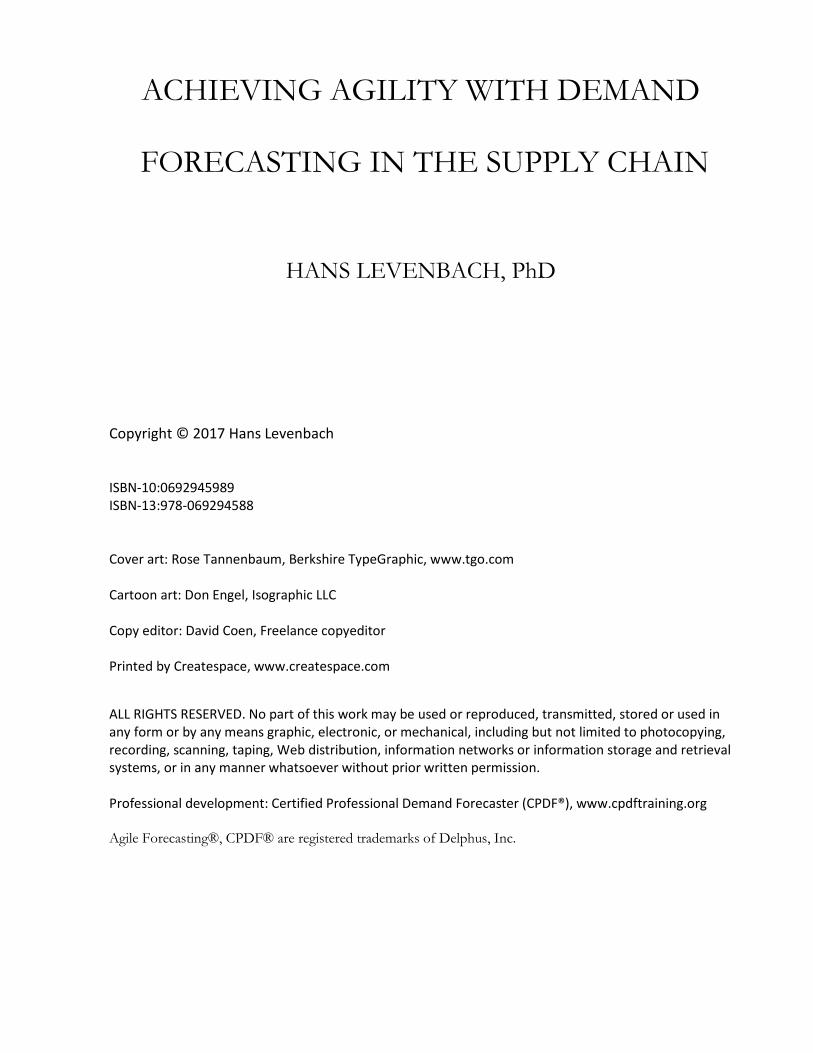
Forecast Profiles for Exponential Smoothing Methods
A system of exponential smoothing models can be classified by the type of trend and/or
seasonal pattern generated as the forecast profile. The most appropriate technique to use
for any forecasting should match the profile expected or desired in an application. Figure
8.7 shows the extended Pegels classification for 12 forecasting profiles for exponential
smoothing developed by Everette S. Gardner, left, in a seminal paper Exponential
smoothing: The state of the art, Journal of Forecasting. 1985.
A Pegels classification of exponential smoothing methods gives rise to 12 forecast
profiles for trend and seasonal patterns.
After a preliminary examination of the data from a time plot, we may be able to determine which of
the dozen models seems most suitable. In Figure 8.7, there are four types of trends to choose from
(Nonseasonal column), and two types of seasonality (Additive and Multiplicative).
Each profile can be directly associated with a specific exponential smoothing model (Figure 8.8), as
described the in the next section (some of which are referred to by a common name attributed to their
authors). We now explain how each model works to generate forecasts; that is, we describe how each
model produces the appropriate forecasting profile.
For a downwardly trending time series, multiplicative seasonality appears as steadily
diminishing swings about a trend. For level data, the constant-level multiplicative and additive
seasonality techniques give the same forecast profile.
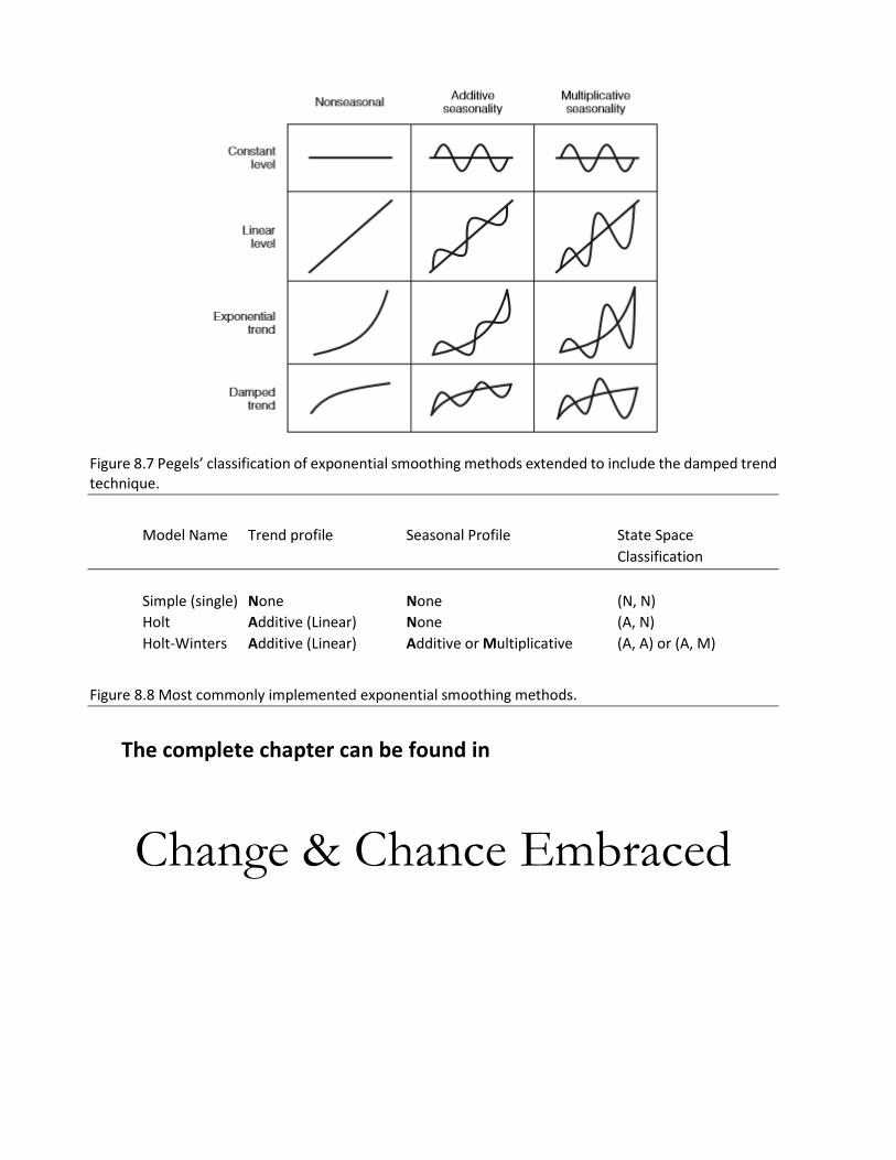
Figure 8.7 Pegels’ classification of exponential smoothing methods extended to include the damped trend
technique.
Model Name Trend profile Seasonal Profile State Space
Classification
Simple (single) None None (N, N)
Holt Additive (Linear) None (A, N)
Holt-Winters Additive (Linear) Additive or Multiplicative (A, A) or (A, M)
Figure 8.8 Most commonly implemented exponential smoothing methods.
The complete chapter can be found in
Change & Chance Embraced
ACHIEVING AGILITY WITH DEMAND
FORECASTING IN THE SUPPLY CHAIN
HANS LEVENBACH, PhD
Copyright © 2017 Hans Levenbach
ISBN-10:0692945989
ISBN-13:978-069294588
Cover art: Rose Tannenbaum, Berkshire TypeGraphic, www.tgo.com
Cartoon art: Don Engel, Isographic LLC
Copy editor: David Coen, Freelance copyeditor
Printed by Createspace, www.createspace.com
ALL RIGHTS RESERVED. No part of this work may be used or reproduced, transmitted, stored or used in
any form or by any means graphic, electronic, or mechanical, including but not limited to photocopying,
recording, scanning, taping, Web distribution, information networks or information storage and retrieval
systems, or in any manner whatsoever without prior written permission.
Professional development: Certified Professional Demand Forecaster (CPDF®), www.cpdftraining.org
Agile Forecasting®, CPDF® are registered trademarks of Delphus, Inc.
Contents :
Chapter 1 - Embracing Change & Chance .............................
Inside the Crystal Ball Error! Bookmark not defined.
Determinants of Demand
Demand Forecasting Defined
Why Demand Forecasting?
The Role of Demand Forecasting in a Consumer-Driven Supply Chain 4
Is Demand Forecasting Worthwhile? 7
Who Are the End Users of Demand Forecasts in the Supply Chain? 8
Learning from Industry Examples 9
Examples of Product Demand 10
Is a Demand Forecast Just a Number? 11
Creating a Structured Forecasting Process 14
The PEER Methodology: A Structured Demand Forecasting Process 14
Case Example: A Consumer Electronics Company 15
PEER Step 1: Identifying Factors Likely to Affect Changes in Demand 16
The GLOBL Product Lines 17
The Marketplace for GLOBL Products 18
Step 2: Selecting a Forecasting Technique 19
Step 3: Executing and Evaluating Forecasting Models22
Step 4: Reconciling Final Forecasts 22
Creating Predictive Visualizations 22
Takeaways 26
Chapter 2 - Demand Forecasting Is Mostly about Data:
Improving Data Quality through Data Exploration and Visualization ............... 28
Demand Forecasting Is Mostly about Data 29
Exploring Data Patterns 29
Learning by Looking at Data Patterns 30
Judging the Quality of Data 30
Data Visualization 35
Time Plots 35
Scatter Diagrams 36
Displaying Data Distributions 37
Overall Behavior of the Data 38
Stem-and-Leaf Displays 39
Box Plots 41
Quantile-Quantile Plots 43
Creating Data Summaries 44
Typical Values 44
The Trimmed Mean 45
Variability 45
Median Absolute Deviation from the Median 45
The Interquartile Difference 46
Detecting Outliers with Resistant Measures 47
The Need for Nonconventional Methods 48
M-Estimators 49
A Numerical Example 49
Why Is Normality So Important? 51
Case Example: GLOBL Product Line B Sales in Region A 52
Takeaways 54
Chapter 3 - Predictive Analytics: Selecting Useful Forecasting Techniques .................................................................................................. 55
All Models Are Wrong. Some Are Useful 56
Qualitative Methods 56
Quantitative Approaches 59
Self-Driven Forecasting Techniques 60
Combining Forecasts is a Useful Method 61
Informed Judgment and Modeling Expertise 62
A Multimethod Approach to Forecasting 64
Some Supplementary Approaches 64
Market Research 64
New Product Introductions 65
Promotions and Special Events 65
Sales Force Composites and Customer Collaboration 65
Neural Nets for Forecasting 66
A Product Life-Cycle Perspective 66
A Prototypical Forecasting Technique: Smoothing Historical Patterns 68
Forecasting with Moving Averages 69
Fit versus Forecast Errors 71
Weighting Based on the Most Current History 73
A Spreadsheet Example: How to Forecast with Weighted Averages 75
Choosing the Smoothing Weight 78
Forecasting with Limited Data 78
Evaluating Forecasting Performance 79
Takeaways 79
Chapter 4 - Taming Uncertainty: What You Need to Know about Measuring Forecast Accuracy ..................................................................................... 80
The Need to Measure Forecast Accuracy 82
Analyzing Forecast Errors 82
Lack of Bias 82
What Is an Acceptable Precision? 83
Ways to Evaluate Accuracy 86
The Fit Period versus the Holdout Period 86
Goodness of Fit versus Forecast Accuracy 87
Item Level versus Aggregate Performance 88
Absolute Errors versus Squared Errors 88
Measures of bias 89
Measures of Precision 90
Comparing with Naive Techniques 93
Relative Error Measures 94
The Myth of the MAPE . . . and How to Avoid It 95
Are There More Reliable Measures Than the MAPE? 96
Predictive Visualization Techniques 96
Ladder Charts 96
Prediction-Realization Diagram 97
Empirical Prediction Intervals for Time Series Models 100
Prediction Interval as a Percentage Miss 101
Prediction Intervals as Early Warning Signals 101
Trigg Tracking Signal 103
Spreadsheet Example: How to Monitor Forecasts 104
Mini Case: Accuracy Measurements of Transportation Forecasts 107
Takeaways 112
Chapter 5 - Characterizing Demand Variability: Seasonality, Trend, and the Uncertainty Factor 114
Visualizing Components in a Time Series 115
Trends and Cycles 116
Seasonality 119
Irregular or Random Fluctuations 122
Weekly Patterns 124
Trading-Day Patterns 124
Exploring Components of Variation 126
Contribution of Trend and Seasonal Effects 127
A Diagnostic Plot and Test for Additivity 130
Unusual Values Need Not Look Big or Be Far Out 132
The Ratio-to-Moving-Average Method 134
Step 1: Trading-Day Adjustment 135
Step 2: Calculating a Centered Moving Average 135
Step 3: Trend-cycle and Seasonal Irregular Ratios 136
Step 4: Seasonally Adjusted Data 137
GLOBL Case Example: Is the Decomposition Additive or Not? 137
APPENDIX: A Two-Way ANOVA Table Analysis 139
Percent Contribution of Trend and Seasonal Effects 140
Takeaways 140
Chapter 6 - Dealing with Seasonal Fluctuations ..................... 141
Seasonal Influences 141
Removing Seasonality by Differencing 143
Seasonal Decomposition 145
Uses of Sasonal Adjustment 146
Multiplicative and Additive Seasonal Decompositions 146
Decomposition of Monthly Data 146
Decomposition of Quarterly Data 151
Seasonal Decomposition of Weekly Point-of-Sale Data 153
Census Seasonal Adjustment Method 156
The Evolution of the X-13ARIMA-SEATS Program 157
Why Use the X-13ARIMA-SEATS Seasonal Adjustment Program? 157
A Forecast Using X-13ARIMA-SEATS 158
Resistant Smoothing 158
Mini Case: A PEER Demand Forecasting Process for Turkey Dinner Cost 162
Takeaways 168
Chapter 7 - Trend-Cycle Forecasting with Turning Points ......... 171
Demand Forecasting with Economic Indicators 171
Origin of Leading Indicators 174
Use of Leading Indicators 174
Composite Indicators 176
Reverse Trend Adjustment of the Leading Indicators 176
Sources of Indicators 178
Selecting Indicators 178
Characterizing Trending Data Patterns 180
Autocorrelation Analysis 180
First Order utocorrelation 182
The Correlogram 183
Trend-Variance Analysis 187
Using Pressures to Analyze Business Cycles 189
Mini Case: Business Cycle Impact on New Orders for Metalworking Machinery 191
1/12 Pressures 192
3/12 Pressures 193
12/12 Pressures 193
Turning Point Forecasting 194
Ten-Step Procedure for a Turning-Point Forecast 195
Alternative Approaches to Turning-Point Forecasting 195
Takeaways 196
Chapter 8 - Big Data: Baseline Forecasting With Exponential Smoothing Models ........................................................................................................ 197
What is Exponential Smoothing? 198
Smoothing Weights 199
The Simple Exponential Smoothing Method 201
Forecast Profiles for Exponential Smoothing Methods 202
Smoothing Levels and Constant Change 204
Damped and Exponential Trends 208
Some Spreadsheet Examples 210
Trend-Seasonal Models with Prediction Limits 216
The Pegels Classification for Trend-Seasonal Models 219
Outlier Adjustment with Prediction Limits 221 Predictive Visualization of Change and Chance – Hotel/Motel Demand 221
Takeaways 225
Chapter 9 - Short-Term Forecasting with ARIMA Models . 226
Why Use ARIMA Models for Forecasting? 226
The Linear Filter Model as a Black Box 227
A Model-Building Strategy 229
Identification: Interpreting Autocorrelation and Partial Autocorrelation Functions 230
Autocorrelation and Partial Autocorrelation Functions 231
An Important Duality Property 233
Seasonal ARMA Process 234
Identifying Nonseasonal ARIMA Models 236
Identification Steps 236
Models for Forecasting Stationary Time Series 236
White Noise and the Autoregressive Moving Average Model 237
One-Period Ahead Forecasts 239
L-Step-Ahead Forecasts 239
Three Kinds of Short-Term Trend Models 241
A Comparison of an ARIMA (0, 1, 0) Model and a Straight-Line Model 241
Seasonal ARIMA Models 244
A Multiplicative Seasonal ARIMA Model 244
Identifying Seasonal ARIMA Models 246
Diagnostic Checking: Validating Model Adequacy 247
Implementing a Trend/Seasonal ARIMA Model for Tourism Demand 249
Preliminary Data Analysis 249
Step 1: Identification 250
Step 2: Estimation 250
Step 3: Diagnostic Checking 251
ARIMA Modeling Checklist 254
Takeaways 255
Postcript 256
Chapter 10 - Demand Forecasting with Regression Models 258
What Are Regression Models? 259
The Regression Curve 260
A Simple Linear Model 260
The Least-Squares Assumption 260
CASE: Sales and Advertising of a Weight Control Product 262
Creating Multiple Linear Regression Models 263
Some Examples 264
CASE: Linear Regression with Two Explanatory Variables 266
Assessing Model Adequacy 268
Transformations and Data Visualization 268
Achieving Linearity 269
Some Perils in Regression Modeling 270
Indicators for Qualitative Variables 273
Use of Indicator Variables 273
Qualitative Factors 274
Dummy Variables for Different Slopes and Intercepts 275
Measuring Discontinuities 275
Adjusting for Seasonal Effects 276
Eliminating the Effects of Outliers 276
How to Forecast with Qualitative Variables 277
Modeling with a Single Qualitative Variable 278
Modeling with Two Qualitative Variables 279
Modeling with Three Qualitative Variables 279
A Multiple Linear Regression Checklist 281
Takeaways 282
Chapter 11 - Gaining Credibility Through Root-Cause Analysis and Exception Handling 283
The Diagnostic Checking Process in Forecasting ............................................................ 284
The Role of Correlation Analysis in Regression Modeling .............................................. 284
Linear Association and Correlation 285
The Scatter Plot Matrix 286
The Need for Outlier Resistance in Correlation Analysis 287
Using Elasticities 288
Price Elasticity and Revenue Demand Forecasting 290
Cross-Elasticity 291
Other Demand Elasticities 292
Estimating Elasticities 292
Validating Modeling Assumptions: A Root-Cause Analysis 293
A Run Test for Randomness 296
Nonrandom Patterns 297
Graphical Aids 299
Identifying Unusual Patterns 299
Exception Handling: The Need for Robustness in Regression Modeling 301
Why Robust Regression? 301
M-Estimators 301
Calculating M-Estimates 302
Using Rolling Forecast Simulations 304
Choosing the Holdout Period 304
Rolling Origins 305
Measuring Forecast Errors over Lead Time 306
Mini Case: Estimating Elasticities and Promotion Effects 306
Procedure 308
Taming Uncertainty 310
Multiple Regression Checklist 311
Takeaways 313
Chapter 12 - The Final Forecast Numbers: Reconciling Change & Chance ..................................................................................................................... 316
Establishing Credibility 317
Setting Down Basic Facts: Forecast Data Analysis and Review 317
Establishing Factors Affecting Future Demand 318
Determining Causes of Change and Chance 318
Preparing Forecast Scenarios 318
Analyzing Forecast Errors 319
Taming Uncertainty: A Critical Role for Informed Judgment 320
Forecast Adjustments: Reconciling Sales Force and Management Overrides 321
Combining Forecasts and Methods 322
Verifying Reasonableness 323
Selecting ‘Final Forecast’ Numbers 324
Gaining Acceptance from Management 325
The Forecast Package 325
Forecast Presentations 326
Case: Creating a Final Forecast for the GLOBL Company 328
Step 1: Developing Factors 329
Impact Change Matrix for the Factors Influencing Product Demand 330
The Impact Association Matrix for the Chosen Factors 331
Exploratory Data Analysis of the Product Line and Factors Influencing Demand 332
Step 2: Creating Univariate and Multivariable Models for Product Lines 334
Handling Exceptions and Forecast Error Analysis 335
Combining Forecasts from Most Useful Models 337
An Unconstrained Baseline Forecast for GLOBL Product Line B, Region A 338
Step 3: Evaluating Model Performance Summaries 341
Step 4: Reconciling Model Projections with Informed Judgment 342
Takeaways 343
Chapter 13 - Creating a Data Framework for Agile Forecasting and Demand Management ................................................................................. 344
Demand Management in the Supply Chain 345
Data-Driven Demand Management Initiatives 346
Demand Information Flows 347
Creating Planning Hierarchies for Demand Forecasting 349
What Are Planning Hierarchies? 349
Operating Lead Times 350
Distribution Resource Planning (DRP)—A Time-Phased Planned Order Forecast 350
Spreadsheet Example: How to Create a Time-Phased Replenishment Plan 352
A Framework for Agility in Forecast Decision Support Functions 353
The Need for Agile Demand Forecasting 354
Dimensions of Demand 354
A Data-Driven Forecast Decision Support Architecture 355
Dealing with Cross-Functional Forecasting Data Requirements 358
Specifying Customer/Location Segments and Product Hierarchies 358
Automated Statistical Models for Baseline Demand Forecasting 360
Selecting Useful Models Visually 363
Searching for Optimal Smoothing Procedures 367
Error-Minimization Criteria 368
Searching for Optimal Smoothing Weights 368
Starting Values 368
Computational Support for Management Overrides 369
Takeaways 372
Chapter 14 - Blending Agile Forecasting with an Integrated Business Planning Process 373
PEERing into the Future: A Framework for Agile Forecasting in Demand Management 374
The Elephant and the Rider Metaphor 374
Prepare 374
Execute 376
Evaluate 376
Reconcile 381
Creating an Agile Forecasting Implementation Checklist 385
Selecting Overall Goals 385
Obtaining Adequate Resources 386
Defining Data 386
Forecast Data Management 387
Selecting Forecasting Software 387
Forecaster Training 388
Coordinating Modeling Efforts 388
Documenting for Future Reference 388
Presenting Models to Management 389
Engaging Agile Forecasting Decision Support 389
Economic/Demographic Data and Forecasting Services 389
Data and Database Management 390
Modeling Assistance 390
Training Workshops 390
The Forecast Manager’s Checklists 391
Forecast Implementation Checklist 391
Software Selection Checklist 392
Large-Volume Demand Forecasting Checklist 393
Takeaways 394


![Forecasting using - Rob J Hyndman exponential smoothing Forecasting using R Simple exponential smoothing 9 animation by animate[2012/05/24] Simple exponential smoothing Optimization](https://img.pdfslide.net/doc/110x75/5aae58377f8b9a07498bfac5/forecasting-using-rob-j-hyndman-exponential-smoothing-forecasting-using-r-simple.jpg)