Big Data Infrastructure

Week 8: Data Mining (2/4)

This work is licensed under a Creative Commons Attribution-Noncommercial-Share Alike 3.0 United StatesSee http://creativecommons.org/licenses/by-nc-sa/3.0/us/ for details

CS 489/698 Big Data Infrastructure (Winter 2017)

Jimmy LinDavid R. Cheriton School of Computer Science

University of Waterloo

March 2, 2017

These slides are available at http://lintool.github.io/bigdata-2017w/

The Task

Given: D = {(xi, yi)}ni(sparse) feature vector

label

xi = [x1, x2, x3, . . . , xd]

y 2 {0, 1}

Induce:Such that loss is minimized

f : X ! Y

1

n

nX

i=0

`(f(xi), yi)

loss function

Typically, we consider functions of a parametric form:

argmin✓

1

n

nX

i=0

`(f(xi; ✓), yi)

model parameters

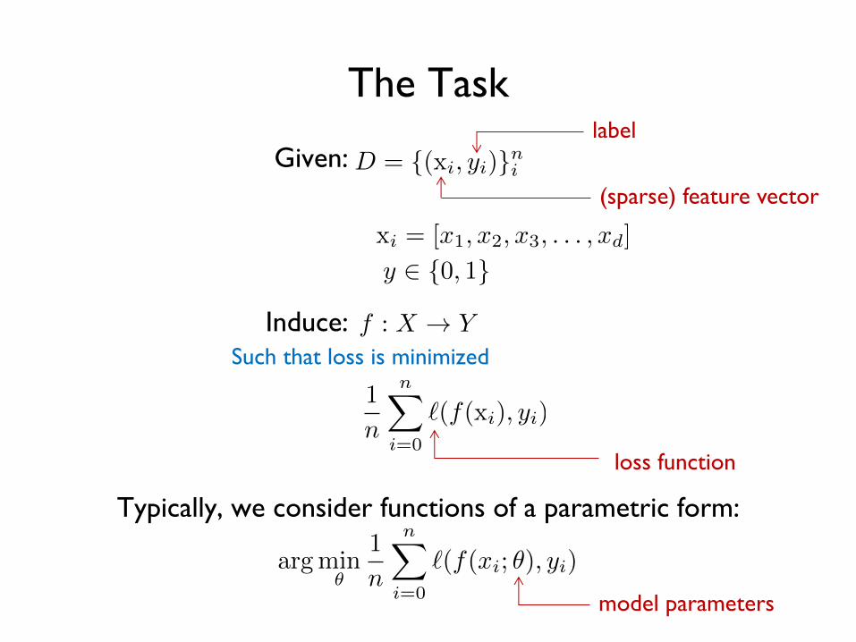
Gradient Descent

Source: Wikipedia (Hills)

✓(t+1) ✓(t) � �(t) 1

n

nX

i=0

r`(f(xi; ✓(t)), yi)

mapper mapper mapper mapper

reducer

compute partial gradient

single reducer

mappers

update model iterate until convergence

✓(t+1) ✓(t) � �(t) 1

n

nX

i=0

r`(f(xi; ✓(t)), yi)

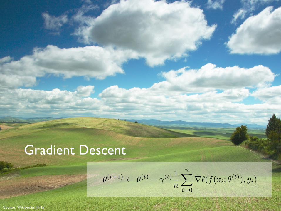
MapReduce Implementation

val points = spark.textFile(...).map(parsePoint).persist()

var w = // random initial vectorfor (i <- 1 to ITERATIONS) {

val gradient = points.map{ p =>p.x * (1/(1+exp(-p.y*(w dot p.x)))-1)*p.y

}.reduce((a,b) => a+b)w -= gradient

}

mapper mapper mapper mapper

reducer

compute partial gradient

update model

Spark Implementation

Gradient Descent

Source: Wikipedia (Hills)

Stochastic Gradient Descent

Source: Wikipedia (Water Slide)

Gradient Descent

Stochastic Gradient Descent (SGD)

✓(t+1) ✓(t) � �(t) 1

n

nX

i=0

r`(f(xi; ✓(t)), yi)

✓(t+1) ✓(t) � �(t)r`(f(x; ✓(t)), y)

Batch vs. Online

“batch” learning: update model after considering all training instances

“online” learning: update model after consideringeach (randomly-selected) training instance

In practice… just as good!Opportunity to interleaving prediction and learning!

We’ve solved the iteration problem!What about the single reducer problem?

Practical Notes

Order of the instances important!Most common implementation: randomly shuffle training instances

Mini-batching as a middle ground

Single vs. multi-pass approaches

Source: Wikipedia (Orchestra)

Ensembles

Ensemble Learning

Common implementation:Train classifiers on different input partitions of the data

Embarrassingly parallel!

Learn multiple models, combine results fromdifferent models to make prediction

Combining predictions:Majority voting

Simple weighted voting:

y = argmax

y2Y

nX

k=1

↵kpk(y|x)

Model averaging…

Ensemble Learning

Why does it work?If errors uncorrelated, multiple classifiers being wrong is less likely

Reduces the variance component of error

Learn multiple models, combine results fromdifferent models to make prediction

✓(t+1) ✓(t) � �(t)r`(f(x; ✓(t)), y)

training data training data training data training data

mapper mapper mapper mapperlearner learner learner learner

MapReduce Implementation

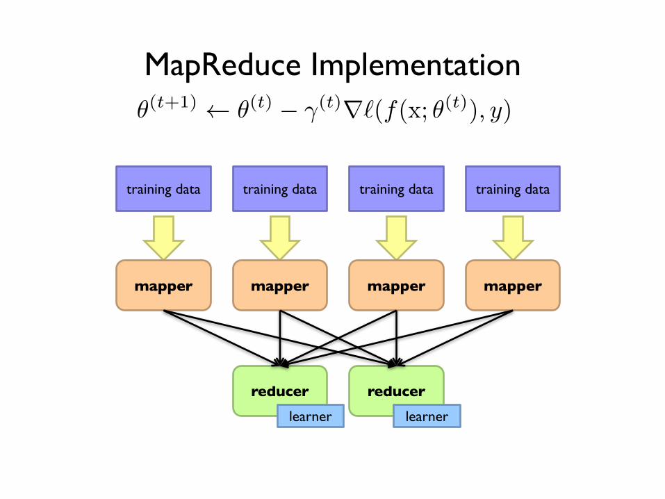
training data training data training data training data

mapper mapper mapper mapper

reducer reducerlearner learner

✓(t+1) ✓(t) � �(t)r`(f(x; ✓(t)), y)MapReduce Implementation

✓(t+1) ✓(t) � �(t)r`(f(x; ✓(t)), y)MapReduce Implementation

How do we output the model?Option 1: write model out as “side data”

Option 2: emit model as intermediate output

✓(t+1) ✓(t) � �(t)r`(f(x; ✓(t)), y)

mapPartitionsf: (Iterator[T]) ⇒ Iterator[U]

RDD[T]

RDD[U]

learner

What about Spark?

Classifier Training

MakingPredictions

Just like any other parallel Pig dataflow

label, feature vector

model UDF

feature vector

prediction

model UDF

feature vector

prediction

model

previous Pig dataflow

map

reduce

previous Pig dataflow

model model

Pig storage function

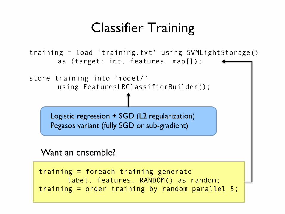
training = load ‘training.txt’ using SVMLightStorage()as (target: int, features: map[]);

store training into ‘model/’using FeaturesLRClassifierBuilder();

Want an ensemble?

training = foreach training generatelabel, features, RANDOM() as random;

training = order training by random parallel 5;

Logistic regression + SGD (L2 regularization)Pegasos variant (fully SGD or sub-gradient)

Classifier Training

define Classify ClassifyWithLR(‘model/’);data = load ‘test.txt’ using SVMLightStorage()

as (target: double, features: map[]);data = foreach data generate target,

Classify(features) as prediction;

Want an ensemble?

define Classify ClassifyWithEnsemble(‘model/’,‘classifier.LR’, ‘vote’);

Making Predictions

Source: Lin and Kolcz. (2012) Large-Scale Machine Learning at Twitter. SIGMOD.

Sentiment Analysis Case Study

Binary polarity classification: {positive, negative} sentimentUse the “emoticon trick” to gather data

DataTest: 500k positive/500k negative tweets from 9/1/2011

Training: {1m, 10m, 100m} instances from before (50/50 split)

Features:Sliding window byte-4grams

Models + Optimization:Logistic regression with SGD (L2 regularization)

Ensembles of various sizes (simple weighted voting)

0.75

0.76

0.77

0.78

0.79

0.8

0.81

0.82

1 1 1 3 5 7 9 11 13 15 17 19 3 5 11 21 31 41

Acc

ura

cy

Number of Classifiers in Ensemble

1m instances10m instances

100m instances

“for free”

Ensembles with 10m examplesbetter than 100m single classifier!

Diminishing returns…

single classifier 10m ensembles 100m ensembles

training

Model

Machine Learning Algorithm

testing/deployment

?

Supervised Machine Learning

EvaluationHow do we know how well we’re doing?

Induce:Such that loss is minimized

f : X ! Y

We need end-to-end metrics!Obvious metric: accuracy

argmin✓

1

n

nX

i=0

`(f(xi; ✓), yi)

Metrics

True Positive (TP)

True Negative (TN)

False Positive (FP)

= Type 1 Error

False Negative(FN)

= Type 1I Error

Actual

Pred

icte

dPositive Negative

Posi

tive

Neg

ativ

e

Precision = TP/(TP + FP)

Miss rate= FN/(FN + TN)

Recall or TPR= TP/(TP + FN)

Fall-Out or FPR= FP/(FP + TN)

ROC and PR CurvesThe Relationship Between Precision-Recall and ROC Curves

0

0.2

0.4

0.6

0.8

1

0 0.2 0.4 0.6 0.8 1

True Positive Rate

False Positive Rate

Algorithm 1Algorithm 2

(a) Comparison in ROC space

0

0.2

0.4

0.6

0.8

1

0 0.2 0.4 0.6 0.8 1Precision

Recall

Algorithm 1Algorithm 2

(b) Comparison in PR space

Figure 1. The difference between comparing algorithms in ROC vs PR space

tween these two spaces, and whether some of the in-teresting properties of ROC space also hold for PRspace. We show that for any dataset, and hence afixed number of positive and negative examples, theROC curve and PR curve for a given algorithm con-tain the “same points.” Therefore the PR curves forAlgorithm I and Algorithm II in Figure 1(b) are, in asense that we formally define, equivalent to the ROCcurves for Algorithm I and Algorithm II, respectivelyin Figure 1(a). Based on this equivalence for ROC andPR curves, we show that a curve dominates in ROCspace if and only if it dominates in PR space. Sec-ond, we introduce the PR space analog to the convexhull in ROC space, which we call the achievable PRcurve. We show that due to the equivalence of thesetwo spaces we can efficiently compute the achievablePR curve. Third we demonstrate that in PR spaceit is insufficient to linearly interpolate between points.Finally, we show that an algorithm that optimizes thearea under the ROC curve is not guaranteed to opti-mize the area under the PR curve.

2. Review of ROC and Precision-Recall

In a binary decision problem, a classifier labels ex-amples as either positive or negative. The decisionmade by the classifier can be represented in a struc-ture known as a confusion matrix or contingency ta-ble. The confusion matrix has four categories: Truepositives (TP) are examples correctly labeled as posi-tives. False positives (FP) refer to negative examplesincorrectly labeled as positive. True negatives (TN)correspond to negatives correctly labeled as negative.Finally, false negatives (FN) refer to positive examplesincorrectly labeled as negative.

A confusion matrix is shown in Figure 2(a). The con-fusion matrix can be used to construct a point in eitherROC space or PR space. Given the confusion matrix,we are able to define the metrics used in each spaceas in Figure 2(b). In ROC space, one plots the FalsePositive Rate (FPR) on the x-axis and the True Pos-itive Rate (TPR) on the y-axis. The FPR measuresthe fraction of negative examples that are misclassi-fied as positive. The TPR measures the fraction ofpositive examples that are correctly labeled. In PRspace, one plots Recall on the x-axis and Precision onthe y-axis. Recall is the same as TPR, whereas Pre-cision measures that fraction of examples classified aspositive that are truly positive. Figure 2(b) gives thedefinitions for each metric. We will treat the metricsas functions that act on the underlying confusion ma-trix which defines a point in either ROC space or PRspace. Thus, given a confusion matrix A, RECALL(A)returns the Recall associated with A.

3. Relationship between ROC Spaceand PR Space

ROC and PR curves are typically generated to evalu-ate the performance of a machine learning algorithmon a given dataset. Each dataset contains a fixed num-ber of positive and negative examples. We show herethat there exists a deep relationship between ROC andPR spaces.

Theorem 3.1. For a given dataset of positive andnegative examples, there exists a one-to-one correspon-dence between a curve in ROC space and a curve in PRspace, such that the curves contain exactly the sameconfusion matrices, if Recall ̸= 0.

Source: Davis and Goadrich. (2006) The Relationship Between Precision-Recall and ROC curves

AUC

Training

Test

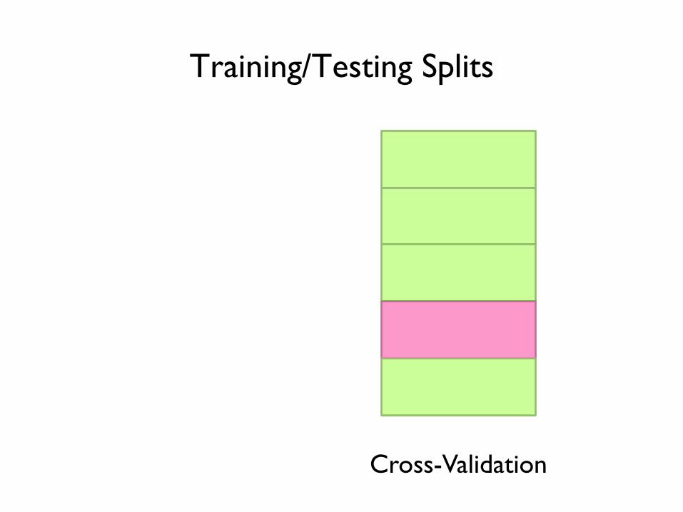
Cross-Validation

Training/Testing Splits

argmin✓

1

n

nX

i=0

`

(f(xi; ✓),yi)

Cross-Validation

Training/Testing Splits

Cross-Validation

Training/Testing Splits

Cross-Validation

Training/Testing Splits

Cross-Validation

Training/Testing Splits

Cross-Validation

Training/Testing Splits

Typical Industry Setup

Training Test

A/B test

time

A/B Testing

Control

Gather metrics, compare alternatives

X %

Treatment

100 - X %

A/B Testing: Complexities

Properly bucketing users

Novelty

Learning effects

Long vs. short term effects

Multiple, interacting tests

Nosy tech journalists

…

training

Model

Machine Learning Algorithm

testing/deployment

?

Supervised Machine Learning

Applied ML in Academia

Download interesting dataset (comes with the problem)

Run baseline modelTrain/Test

Build better modelTrain/Test

Does new model beat baseline?Yes: publish a paper!

No: try again!

Fantasy

Extract features

Develop cool ML technique

#Profit

Reality

What’s the task?

Where’s the data?

What’s in this dataset?

What’s all the f#$!* crap?

Clean the data

Extract features

“Do” machine learning

Fail, iterate…

It’s impossible to overstress this: 80% of the work in any data project is in cleaning

the data. – DJ Patil “Data Jujitsu”

Source: Wikipedia (Jujitsu)

On finding things…

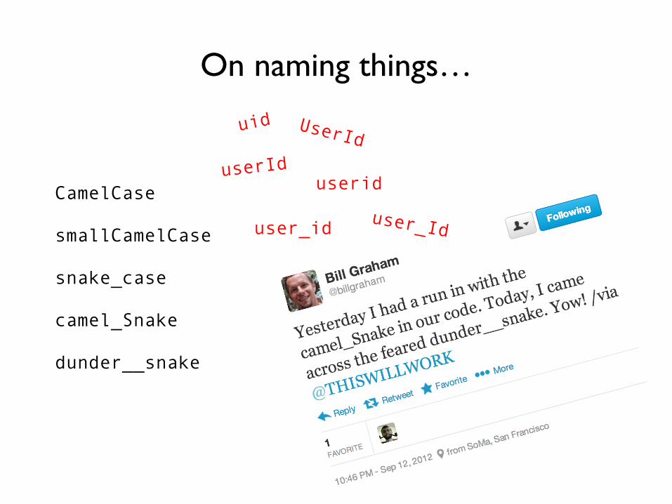
CamelCase

smallCamelCase

snake_case

camel_Snake

dunder__snake

userid

user_id

On naming things…

^(\\w+\\s+\\d+\\s+\\d+:\\d+:\\d+)\\s+([^@]+?)@(\\S+)\\s+(\\S+):\\s+(\\S+)\\s+(\\S+)\\s+((?:\\S+?,\\s+)*(?:\\S+?))\\s+(\\S+)\\s+(\\S+)\\s+\\[([^\\]]+)\\]\\s+\"(\\w+)\\s+([^\"\\\\]*(?:\\\\.[^\"\\\\]*)*)\\s+(\\S+)\"\\s+(\\S+)\\s+(\\S+)\\s+\"([^\"\\\\]*(?:\\\\.[^\"\\\\]*)*)\"\\s+\"([^\"\\\\]*(?:\\\\.[^\"\\\\]*)*)\"\\s*(\\d*-[\\d-]*)?\\s*(\\d+)?\\s*(\\d*\\.[\\d\\.]*)?(\\s+[-\\w]+)?.*$

An actual Java regular expression used to parse log message at Twitter circa 2010

Friction is cumulative!

On feature extraction…

Frontend EngineerDevelops new feature, adds logging code to capture clicks

Data ScientistAnalyze user behavior, extract insights to improve feature

Okay, let’s get going… where’s the click data?

Well, that’s kinda non-intuitive, but okay…

Oh, BTW, where’s the timestamp of the click?

It’s over here…

Well, it wouldn’t fit, so we had to shoehorn…

Hang on, I don’t remember…

Uh, bad news. Looks like we forgot to log it…

[grumble, grumble, grumble]

…

Data Plumbing… Gone Wrong![scene: consumer internet company in the Bay Area…]

Extract features

Develop cool ML technique

#Profit

What’s the task?

Where’s the data?

What’s in this dataset?

What’s all the f#$!* crap?

Clean the data

Extract features

“Do” machine learning

Fail, iterate…

Fantasy Reality

Source: Wikipedia (Hills)

Congratulations, you’re halfway there…

Does it actually work?

Congratulations, you’re halfway there…

Is it fast enough?

Good, you’re two thirds there…

A/B testing

Source: Wikipedia (Oil refinery)

Productionize

What are your jobs’ dependencies?

How/when are your jobs scheduled?

Infrastructure is critical here!

Are there enough resources?

How do you know if it’s working?

Who do you call if it stops working?

(plumbing)

Productionize

Source: Wikipedia (Plumbing)

Most of data science isn’t glamorous!Takeaway lessons:

Source: Wikipedia (Japanese rock garden)

Questions?