Embed Size (px)
Citation preview
YuMi Deadly Mathematics
Big Ideas of Mathematics
Prep to Year 12
Prepared by the YuMi Deadly Centre Queensland University of Technology
Kelvin Grove, Queensland, 4059
Prep
to Y
ear 1
2: S
upp
lem
enta
ry R
esou
rce
1 –
Big
Idea
s of
Mat
hem
atic
s

YuMi Deadly Mathematics
Big Ideas of Mathematics
DRAFT 5/03/16
Prepared by the YuMi Deadly Centre Queensland University of Technology
Kelvin Grove, Queensland, 4059
http://ydc.qut.edu.au
© 2016 Queensland University of Technology through the YuMi Deadly Centre
Page ii Big Ideas of Mathematics 5/03/2016 © QUT YuMi Deadly Centre 2016
ACKNOWLEDGEMENT
The YuMi Deadly Centre acknowledges the traditional owners and custodians of the lands in which the mathematics ideas for this resource were developed,
refined and presented in professional development sessions.
YUMI DEADLY CENTRE
The YuMi Deadly Centre is a research centre within the Faculty of Education at QUT which is dedicated to enhancing the learning of Indigenous and non-Indigenous children, young people and adults to improve their opportunities for further education, training and employment, and to equip them for lifelong learning.
“YuMi” is a Torres Strait Islander Creole word meaning “you and me” but is used here with permission from the Torres Strait Islanders’ Regional Education Council to mean working together as a community for the betterment of education for all. “Deadly” is an Aboriginal word used widely across Australia to mean smart in terms of being the best one can be in learning and life.
The YuMi Deadly Centre’s motif was developed by Blacklines to depict learning, empowerment, and growth within country/community. The three key elements are the individual (represented by the inner seed), the community (represented by the leaf), and the journey/pathway of learning (represented by the curved line which winds around and up through the leaf). As such, the motif illustrates the YuMi Deadly Centre’s vision: Growing community through education.
The YuMi Deadly Centre can be contacted at [email protected]. Its website is http://ydc.qut.edu.au.
CONDITIONS OF USE AND RESTRICTED WAIVER OF COPYRIGHT
Copyright and all other intellectual property rights in relation to this book (the Work) are owned by the Queensland University of Technology (QUT).
Except under the conditions of the restricted waiver of copyright below, no part of the Work may be reproduced or otherwise used for any purpose without receiving the prior written consent of QUT to do so.
The Work may only be used by certified YuMi Deadly Mathematics trainers at licensed sites that have received professional development as part of a YuMi Deadly Centre project. The Work is subject to a restricted waiver of copyright to allow copies to be made, subject to the following conditions:
1. all copies shall be made without alteration or abridgement and must retain acknowledgement of the copyright;
2. the Work must not be copied for the purposes of sale or hire or otherwise be used to derive revenue;
3. the restricted waiver of copyright is not transferable and may be withdrawn if any of these conditions are breached.
© QUT YuMi Deadly Centre 2016
© QUT YuMi Deadly Centre 2016 5/03/2016 Big Ideas of Mathematics Page iii
Contents
Page
Overview .......................................................................................................................................................... 1 Nature of big ideas .......................................................................................................................................... 1 Cognitive basis of big ideas ............................................................................................................................. 1 Learning of big ideas ....................................................................................................................................... 3 Types of big ideas ............................................................................................................................................ 4 Selection of big ideas ...................................................................................................................................... 5
1 Global Big Ideas ........................................................................................................................................ 9 1.1 Structural ................................................................................................................................................ 9 1.2 Pattern .................................................................................................................................................. 10 1.3 Logical reasoning .................................................................................................................................. 10 1.4 Language............................................................................................................................................... 13 1.5 Problem solving .................................................................................................................................... 15
2 Concept Big Ideas ................................................................................................................................... 17 2.1 Numeration .......................................................................................................................................... 17 2.2 Equality ................................................................................................................................................. 20 2.3 Addition and subtraction ...................................................................................................................... 21 2.4 Multiplication and division ................................................................................................................... 22 2.5 Attributes .............................................................................................................................................. 26 2.6 Patterns and functions ......................................................................................................................... 27 2.7 Shapes .................................................................................................................................................. 29 2.8 Transformations ................................................................................................................................... 31 2.9 Infiniteness ........................................................................................................................................... 32 2.10 Rates ..................................................................................................................................................... 34 2.11 Statistics and probability ...................................................................................................................... 36
3 Principle Big Ideas .................................................................................................................................. 39 3.1 Part–whole–group ................................................................................................................................ 39 3.2 Odometer principle .............................................................................................................................. 39 3.3 Multiplicative structures ...................................................................................................................... 40 3.4 Quantity on number line ...................................................................................................................... 40 3.5 Equals/order properties ....................................................................................................................... 41 3.6 Operation properties ............................................................................................................................ 41 3.7 Inverse .................................................................................................................................................. 43 3.8 Units of measure and instrumentation ................................................................................................ 44 3.9 Formulae............................................................................................................................................... 44
4 Strategy and Modelling Big Ideas ........................................................................................................... 47 4.1 Computation ......................................................................................................................................... 47 4.2 Algebra ................................................................................................................................................. 48 4.3 Measurement ....................................................................................................................................... 49 4.4 Visualising ............................................................................................................................................. 49 4.5 Statistical inference .............................................................................................................................. 52 4.6 Problem solving .................................................................................................................................... 53 4.7 Mathematical modelling ...................................................................................................................... 54
5 Pedagogy Big Ideas ................................................................................................................................. 57 5.1 Structure ............................................................................................................................................... 57 5.2 Sequencing ........................................................................................................................................... 57 5.3 Pedagogical approaches ....................................................................................................................... 58 5.4 RAMR cycle ........................................................................................................................................... 60 5.5 Language and problem solving ............................................................................................................. 63
Page iv Big Ideas of Mathematics 5/03/2016 © QUT YuMi Deadly Centre 2016
5.6 Application of Blooms taxonomy to mathematics ............................................................................... 64 5.7 Pedagogical models used in mathematics ............................................................................................ 65 5.8 Mathematical technology ..................................................................................................................... 69
6 Superstructures: The convergence of big ideas ...................................................................................... 71 6.1 Concept maps ....................................................................................................................................... 71 6.2 Pre-requisite knowledge and skills ....................................................................................................... 71 6.3 Superstructures .................................................................................................................................... 72 6.4 Convergence of big ideas ...................................................................................................................... 72
Appendix A: Summary of Big Ideas ................................................................................................................. 73
Appendix B: Classification of Task Words ....................................................................................................... 74
References ...................................................................................................................................................... 75
© QUT YuMi Deadly Centre 2016 5/03/2016 Big Ideas of Mathematics Page v
YUMI DEADLY CENTRE MATHEMATICS PROJECTS
In late 2009, the YuMi Deadly Centre (YDC) received funding from the Queensland Department of Education and Training (DET) through the Indigenous Schooling Support Unit (ISSU) to develop a train-the-trainer project, called the Teaching Indigenous Mathematics Education or TIME project, to enhance the capacity of Indigenous and low income schools to effectively teach mathematics to their students. This three-year project focused on Years P to 3 in 2010, Years 4 to 7 in 2011 and Years 7 to 9 in 2012, covering all mathematics strands in the Australian Curriculum: Number and Algebra, Measurement and Geometry, and Statistics and Probability. The work of this project enabled YDC to develop a cohesive mathematics pedagogical framework, YuMi Deadly Mathematics (YDM), that now underpins all YDC projects.
YuMi Deadly Mathematics. YDM is designed to enhance mathematics learning outcomes, improve participation in higher mathematics subjects, and improve employment and life chances and participation in tertiary courses. YDM is unique in its focus on creativity, structure and culture with regard to mathematics and on whole-of-school change with regard to implementation. Its underpinning philosophy is very applicable to all schools with high numbers of students at risk, but is equally applicable to all students whatever their performance.
YDM is based on the belief that changing a mathematics program will not improve mathematics learning unless accompanied by a whole-of-school program that challenges attendance and behaviour, encourages pride and self-belief, instils high expectations, and builds local leadership and community involvement. It is strongly influenced by the philosophy of the Stronger Smarter Institute established by Dr Chris Sarra, that any school has the potential to meet the challenges of successfully teaching their students.
YDM projects in YDC. YDM is the basis for all projects in mathematics run by YDC. This covers the following three project areas:
1. Teacher professional learning (PL) projects, mostly called YDM projects, that prepare teachers to effectively use the YDM mathematics materials (predominantly in Indigenous and low income schools).
2. Accelerated Inclusive Mathematics (AIM) that are remedial projects to accelerate learning for very underperforming junior secondary students through the use of modules and a vertical curriculum.
3. Mathematicians in Training Initiative (MITI) projects that are mathematics enrichment and extension projects using YDM approaches to develop extension tasks and a deep learning pedagogy to extend students’ mathematics knowledge to improve participation in Years 11 and 12 advanced mathematics subjects and increase university entrance rates.
YuMi Deadly Mathematics can underpin all these different projects because of its focus on structure through connections, sequencing and big ideas. Big ideas enable acceleration of learning for underperforming students and extension to deeper mathematics for able students. They are a structure around which a Mathematics program for all students can be built.
The role of this resource. This resource is an introductory book about the “big ideas” of mathematics that underpins the YDM pedagogy in all year levels. It describes big ideas in five categories: global; concepts; principles; strategies; and pedagogy. The ideas in this resource have come from reflection on the YDC mathematics projects in 2010–15. They will continue to evolve as YDM is used in projects. Thus this book will be revised regularly.
If you would like to contribute your ideas for the ongoing improvement of this book, please contact Professor Tom Cooper at [email protected] or 07 3138 3331.

© QUT YuMi Deadly Centre 2016 5/03/2016 Big Ideas for Mathematics Page 1
Overview
This book describes the big ideas of mathematics with respect to content, teaching and learning from levels or grades P to 12. This section looks at: (a) what big ideas are (their nature); (b) how they can assist learning; (c) how big ideas can be learnt; (d) the different types of big ideas that are recognised by YuMi Deadly Mathematics (YDM); and (e) how the big ideas are clustered in this book.
Nature of big ideas
Big ideas transcend the various branches of mathematics and also year levels. For YDM, mathematics big ideas are ideas that have some or all of the following properties:
1. Topic generic. They apply across topic areas – they have some generic capabilities with respect to topics and are not restricted to a particular domain (e.g. the inverse relation in division between divisor and quotient also applies to measuring using units, fractions and probability).
2. Level generic. They apply across year levels – they have the capacity to remain meaningful and useful as a learner moves up the grades (e.g. the concept of addition holds for early work in whole numbers, and continues to apply to work in decimals, measurements, variables, vectors and matrices).
3. Content generic. Their meaning is independent of context and content – it is encapsulated in what they are and how they relate, not the particular context in which they operate (e.g. the commutative law says that first plus second = second plus first applies across a wide range of topics including decimals, fractions and functions).
Thus, big ideas are powerful ways to learn mathematics for the following reasons:
1. Power. One big idea can apply to a lot of mathematics (e.g. multiplicative comparison and using start-change-end diagrams can solve most fraction, percent, rate and ratio problems which means less learning than the many procedures taught for these topics in many classrooms).
2. Efficiency. There are many fewer big ideas in mathematics than there are procedures and rules to be rote learnt (e.g. the distributive law and area diagrams can be used to understand and solve 24 × 37, 2/5 × 4/5 and (𝑥𝑥 − 1)(𝑥𝑥 + 2) problems).
3. Organic growth. As they are applied to topics, big ideas build structural connectivity in mathematics that can easily accommodate the next steps in mathematics knowledge and makes later learning of mathematics easier (e.g. building up the notion of inverse as “undoing things” and teaching the inverse relationships between +2 and −2, ×5 and ÷5, 𝑥𝑥2 and √𝑥𝑥, 𝑝𝑝3 and 𝑝𝑝−3, (𝑝𝑝)𝑛𝑛 and (𝑝𝑝)1/𝑛𝑛, 𝑓𝑓(𝑥𝑥) = 2𝑥𝑥 + 1 and 𝑓𝑓(𝑥𝑥) =(𝑥𝑥 − 1) ÷ 2 can make it really easy to understand integration as the inverse of differentiation in calculus).
Cognitive basis of big ideas
The YDM approach to predagogy is underpinned by a social constructivist perspective of teaching and learning in mathematics. Mathematical knowledge is seen as the collaborative invention of people (Vygotsky, 1978) where the importance of culture and context in developing meaning is emphasised. In the context of school mathematics, learning is the aquisition and adaptation of of a set of structured and connected mathematical mentral representations (schemas) by the student (Piaget, 1977), influenced by the student’s personal experiences and by teachers who guide the process (Davydov, 1995; Jardine, 2006). These carefully selected and structured schemas used as a foundation for further learning are the big ideas of mathematics.
Page 2 Overview 5/03/2016 © QUT YuMi Deadly Centre 2016
Piaget (1977) considered that people learn by organising their knowledge into schemas. Learning occurs by increasing the number and complexity of the schemas by adaptation (adjustment) to the world, through two processes called assimilation and accommodation. In the process of assimilation existing schemas are used to interpret new information. The student identifies similarities between the new information and the known schema and then maps them from one to the other, generating plausible inferences about the new information. When the new information cannot be assimilated into existing schemas a state of disequilibrium occurs. To resolve this, existing schemas must be changed or supplemented through the process of accommodation. It follows that learning is easier if assimilation is possible.
Not all schemas are the same. For example, they can be abstract or content-based. Abstract schemas operate as a structure into which content can be slotted (Ohlsson, 1993), in the same way as an on-paper form or computer template can be completed by inserting information into the spaces provided. Teachers often represent abstract schemas to students as graphic organisers. As abstract schemas are independent of content they differ from schemas that depend on particular contexts. On the other hand, concept schema are an individual’s set of representations and properties of a mathematical concept (Niss 2006).
It follows that learning is most efficient if new mathematical concepts are processed by relating them to existing big ideas (assimilation), thereby reducing the need to develop new understandings (accommodation). However, if students fail to develop a relational understanding of mathematics as a framework of connected big ideas, there is a limited foundation to draw on to assimilate new knowledge. The outcome can be a large number of disconnected facts that cannot be generalised and require drill and practice methods to ensure future recall (called instrumental knowledge) (Skemp, 1976).
Mathematical understanding is the connectedness of a student’s internal schema. Connected schemas are developed by finding the structural similarities and differences between mental models which then lead to the development of more abstract models, that is, the big ideas of mathematics. This structured sequencing theory (Cooper & Warren, 2011; Warren & Cooper, 2007) is based on six propositions:
• the processes leading to the development of big ideas follow structured sequences that take account of various mental models and their representations;
• effective mental models and their representations highlight the big idea and are easily extended to new situations;
• an effective structured sequence uses mental models and their representations in increasingly flexible ways, has decreased overt structure, provides increased coverage, and has a form that is related to real-world instances;
• an effective structured sequence ensures that later ideas can be nested in earlier ideas;
• complex procedures that involve the coordination of several parts will give rise to the need for a big idea that integrates the coordinated parts; and
• a big idea is abstracted through the comparison of its various representations.
Big ideas are seen as the central organising ideas (Schifter & Fosnot, 1993) that robustly link many mathematical understandings into a coherent whole (Charles, 2005). They have been characterised as having potential for:
• encouraging learning with understanding of conceptual knowledge;
• developing meta-knowledge about mathematics;
• supporting the ability to communicate meaningfully about mathematics; and
• encouraging the design of rich learning opportunities that support students’ learning processes (Kuntze et al., 2011).
It has been argued that relating new concepts to big ideas promotes understanding, thus enhancing motivation, further understanding, memory, transfer, attitudes and beliefs, and autonomy of learning (Lambdin, 2003).
© QUT YuMi Deadly Centre 2016 5/03/2016 Big Ideas for Mathematics Page 3
To summarise, mathematical ideas are most powerful when they are connected and sequenced into a rich schema. The basis of a rich schema is that it complexly defines an idea, connects the idea to all related ideas, prepares for applications, and is developed from the learner’s experience (guided by the teacher). There are two implications of this. The first is that strong learning comes from following appropriate sequences (e.g. division fraction ratio decimal percent probability) in as seamless a manner as possible. Inadequate learning and understanding is caused by missing parts in the sequence, and thus improving learning requires rebuilding important steps. The second is that, when teaching these sequences, connections should be made between present work and earlier elements, and to other sequences that are related. Mathematics ideas should not be provided in isolation but in relation to other mathematics ideas.
Learning of big ideas
Learning of big ideas is not a “lesson” activity. It has to be planned across the years of schooling. For example, addition is first built informally as joining like things at an early age, then extended to more formal big ideas (e.g. identity, inverse, commutative and associative laws) so that it can be understood when applied to directed number and algebra.
Big ideas are, therefore, built through structured sequences that span across models (ways of thinking about abstract concepts, often metaphorically) and representations (ways of expressing the models, including concretely, pictorially and with written or spoken language). The structured sequences that enhance learning of big ideas have the following properties (Cooper & Warren, 2011):
(a) Effective models and representations. The sequences use models and representations which have a strong isomorphism (same structure) to desired internal mental models, few distracters and many options for extension.
(b) Appropriate order. The sequences use these models and representations in an order that reflects increased flexibility, decreased overt structure, increased coverage and continuous connectedness to reality; and the consecutive steps of the sequence explore ideas which are nested (later thinking is a subset of earlier) wherever possible.
(c) Integration and superstructures. Complexities in the sequences can be ameliorated by integrating models and representations but, if integration leads to compound difficulties (opposite results for close topics, e.g. maintaining the answer requires opposite changes in addition and same changes in subtraction), this may require the development of superstructures (structures that facilitate integration, e.g. subtraction is inverse of addition so we would expect opposite activity when comparing the two).
(d) Comparison and commonalities. The sequences contain models and representations that enable commonalities that represent the kernel of desired internal mental models to be abstracted through comparison of these models and representations.
The Australian Curriculum: Mathematics is not structured around big ideas, with the content arranged in topics and year levels. This presentation is reasonable when the intended audience is teachers with a deep understanding of the structures and connections of mathematics. However, many textbook writers have uncritically adopted the curriculum arrangement for presentation to students who have yet to develop those deep understandings. The textbook structure is then adopted by mathematics teachers as a pedagogical approach, resulting in annual cycles of piecemeal, topic-by-topic approaches using drill and practice methods, subverting students’ understanding of the underlying principles (Schifter & Fosnot, 1993).
The structured sequence approach is facilitated by vertical curriculum. This is where the content to be taught is partitioned into topics (for example, whole number numeration, decimal number numeration and common fraction numeration) and topics are taught vertically with instruction built around units that explore the topics across year levels. This enables instruction to be built around big ideas (e.g. for numeration, these are vertically part-whole, odometer, quantity on a number line, multiplicative structure, and equivalence – see later sections 2 and 3), as well as the normal constituents of mathematical topics, namely, concepts, strategies and principles.
Page 4 Overview 5/03/2016 © QUT YuMi Deadly Centre 2016
Types of big ideas
For YDM, the big ideas of mathematics should cover significant concepts and have a wide effect. Thus, they have some or all of these properties:
• they provide generic approaches to a wide range of ideas, encompassing viewpoints that cross boundaries;
• they apply across topic areas, with some generic capabilities that are not restricted to a particular domain;
• they apply across year levels, with the capacity to remain meaningful and useful as a learner moves up the grades;
• their meaning is independent of context and content, but is encapsulated in what they are and how they relate.
These properties are consistent with the approach proposed by many others. However, YDM argues that, to meet the big ideas criterion of transcending topics and year levels, the big ideas of mathematics should go beyond content in the form of concepts and principles to pedagogical approaches used by teachers and the strategies used in modelling and problem solving. This understanding of big ideas leads to two further properties:
• they can include generic strategies for solving problems or quantitatively modelling the behaviour of systems; and
• they can be pedagogical approaches with the capacity to apply to many situations.
The justification for focusing on this wider range of big ideas is that they provide the basis for more efficient and effective learning of mathematics, for two reasons. First, mathematical knowledge is insufficient without skills. The most important skills of mathematics are the appropriate selection and application of strategies and procedures. Strategies are general rules of thumb that point towards answers in problem situations, differing from procedures that are fixed ways to get an answer with a finite series of steps. Many strategies are generic, for example, mathematical modelling – a strategy big idea that can be applied to a variety of contexts. Second, ideas that are related in some way mathematically are also related pedagogically, that is, they are often taught in a similar manner. Thus, pedagogy big ideas are approaches to teaching mathematics that are generic to most or all teaching of mathematics topics, for example, the pedagogy of reversing where the teaching direction between teacher and student is reversed.
Since not all big ideas are the same, YDM classifies them as five types, each detailed in the sections that follow this overview: global, concept, principle, strategy and modelling, and pedagogy.
Global
Global big ideas are highly generic – they apply across the full range of mathematics. For example, mathematics can be seen in terms of relationships (e.g. 2 and 3 are related to 5 by addition, and two shapes are similar if their angles are equal and their side lengths are in ratio) and in terms of change (e.g. addition changes 2 to 5 by adding 3, and if a shape is changed by enlarging it, then the shapes before and after the change are similar). If this big idea is understood, then every mathematics idea can be considered in terms of relationship and change. It is a global big idea because it gives extra options when solving mathematics problems and is applicable to all topics in mathematics.
Concept
Concept big ideas are the precepts that lie behind all mathematical content, with meanings that are common across mathematics. For example, the understanding that equals as “the same value” has large impact and applies to most, if not all, topics in mathematics.
© QUT YuMi Deadly Centre 2016 5/03/2016 Big Ideas for Mathematics Page 5
Principle
This is where YDM’s interest in big ideas started. Öhlsson (1993) argued that there were two types of relationships: (a) contentful, which is based on specific content such 2 + 3 = 5 for addition; and (b) abstract, where meaning is encapsulated in the relation of the parts not in terms of the content to be used. For example, a law that holds for all numbers like commutativity (e.g. a + b = b + a) has its meaning in the ways a and b are related not in the numerical values assigned to a and b. Öhlsson argued that powerful mathematical understanding was based on seeing mathematics in abstract schema terms.
In mathematics and in YDM, abstract schemas, laws and relationships are known as principles. For example, principle big ideas cover the laws such as distributive and associative, formulae such as the area of a rectangle is the multiplication of length and width, and relationships such as the inverse relation between divisor b and quotient c in division example a ÷ b = c.
Strategy and modelling
Problems are situations where knowledge is not enough for solution (there is a blockage that has to be overcome by applying logic). Strategies are general approaches (or rules of thumb) that point towards answers in problem situations. Strategies differ from procedures because procedures are fixed ways to get an answer with a finite series of steps. Strategies can be thought of as what you do when you don’t know what to do. Strategies tend to be seen in relation to concepts and principles – in fact, these three big ideas are an excellent way to approach the teaching of any mathematics topic area.
Of course the same criteria apply to strategy big ideas as to other big ideas – strategy big ideas must be generic in some way. There are many generic strategies. For example, breaking a problem into parts is a generic strategy. It is used in the process of addition where a number is separated into parts such as ones, tens, hundreds, the parts are added separately and then recombined. It is also used to calculate the area of a complex shape by dividing it into two or more simpler shapes, finding the areas of those simpler shapes, and then adding them to find the area of the original shape. It also applies to complex problems that are broken into steps that are processed sequentially to reach the solution.
Pedagogy
The interesting thing about mathematics is that ideas that are related in some way mathematically are often related pedagogically – that is, they are often taught in a similar manner. Thus, pedagogy big ideas are approaches to teaching mathematics that are generic to most or all teaching of mathematics topics. For example,
The YDM pedagogy is built around generic teaching approaches such as the RAMR cycle. Thus, the last collection of big ideas in this book will be teaching or pedagogy big ideas.
Selection of big ideas
Big ideas have always been a focus of YDM in that they offer a powerful shortcut to learning and retention because of their generic nature, their coverage, and the way they build structure. YDM has included a list of big ideas in its Overview book since 2010. However, this list has consisted of only a few global big ideas and a more extensive list of principle big ideas.
As YDM has grown, it has become evident that the list of big ideas should be broadened. It was obvious that there were many ideas other than principles that were generic across topics, levels and content, for example, the concept of multiplication. Thus, this new book has been prepared. It contains new types of big ideas and extended lists in all types of big ideas.
In preparing this new list, it became evident that it is sometimes difficult to know when an idea moves from small to big, that is, to determine the point at which there is sufficient generic application of an idea to call it big. Taking
Page 6 Overview 5/03/2016 © QUT YuMi Deadly Centre 2016
a liberal approach at this point meant that the number of big ideas grew rapidly to where they became less powerful as a shortcut to learning and retention and more like a restatement of all mathematics topics. Thus, the following was done:
(a) Structure from major idea. The form of the book was reconsidered in terms of the very generic major ideas that affect overall teaching and learning of mathematics, and then the book was structured about these.
(b) Clusters. Particular big ideas were clustered with similar ideas to ensure that the book represented major groupings of ideas (this enables all the big ideas associated, say, with inverse to be seen as a cluster).
(c) Coverage. Big ideas were extended from global and principles to also cover concepts, strategies and pedagogy as well (this allowed some ideas, such as the concept of infiniteness and computation strategies, to take their rightful place as major ideas).
(d) Frameworks. Frameworks that were the basis of YDM’s focus on what and how to teach were added to the list of pedagogy big ideas.
This book
This book is presented in six sections after this overview. The first five sections deal with the big ideas classified as global, conceptual, principle, strategic and pedagogical. The sixth section draws together the big ideas into a consolidated understanding of mathematics. Finally, there is a one-page summary of the big ideas.
A review of the literature about big ideas reveals that, whilst there is agreement about the nature and purpose of a big ideas approach to mathematics, there is little agreement on what the big ideas should be (Carter, 2016). Many approaches have been proposed, often reflecting the stage of education (for example, early years, upper primary, middle years, senior years) that the writer is interested in. The YDM view of big ideas takes account of all years of schooling. This means that the emphasis given to some big ideas may vary according to the stage of schooling (for example, infiniteness may not be an important part of mathematics study in the early years). However, YDM believes that all the ideas proposed in this book are critical to the successful study of mathematics.
Mathematics is a comprehensive and interconnected body of knowledge. It does not easily lend itself to a partitioning into topics or big ideas. Regardless of how it is done, there will always be connections to other parts of mathematics. As students mature mathematically, these connections become more apparent. In recognition of this, the discussion of the big ideas in this book also identifies the connections to other big ideas.
For example, calculus is a higher level application of mathematics. It draws together several conceptual big ideas, including infiniteness (limits), number (measurement), multiplication (rates), shapes (area), and patterns and functions (functions and gradients) and also the principle of an inverse. The large number of connections has several implications:
• it demonstrates the extent of the knowledge that students must have mastered before they are ready for the study of calculus (explaining why it is taught in the upper secondary years);
• it provides opportunities for students to connect the big ideas;
• it provides opportunities for teachers to refresh past content.; and
• a pedagogy that explicitly links calculus to the underlying big ideas is more powerful in developing understanding than one that treats calculus as a stand-alone topic.
The convergence of big ideas as students reach the higher level of mathematics is to be encouraged. The goal is that students will come to view mathematics as the comprehensive and interconnected body of knowledge referred to above. This issue is discussed further in Section 6.

© QUT YuMi Deadly Centre 2016 5/03/2016 Big Ideas for Mathematics Page 7
This book outlines the YDM perspective of big ideas. In each case, the nature and scope of the big idea is explained in sufficient detail to understand what is included. However, it does not seek to explain the mathematical theory in detail – that information is available in other YDM materials and elsewhere.

© QUT YuMi Deadly Centre 2016 5/03/2016 Big Ideas for Mathematics Page 9
1 Global Big Ideas
Global big ideas are highly generic – they apply across the full range of mathematics. YDM has identified five global big ideas. They are clustered for ease of presentation and retention. This clustering is built around the understanding, which is at the basis of YDM, that mathematics has five major characteristics:
(a) structure – mathematics is a structure of sequenced and connected ideas that integrate into a rich schema;
(b) pattern – many define mathematics to be the study of patterns in, and relationships between, quantities and sets;
(c) logical thinking – the foundation of mathematical reasoning;
(d) language – mathematics is a succinct language that describes reality (i.e. the world around us), which includes symbols as a form of “shorthand”; and
(e) tool for problem solving – mathematics is a collection of thinking tools that can help people solve their problems.
1.1 Structural
1.1.1 Change vs relationship
Mathematics has three components – objects, relationships between objects and changes leading to the transformation from one object to another. Object is used here and throughout the book as a generic term that can variously refer to numbers, measurements, lines, angles, shapes, tables, graphs, depending on the context.
Everything can be seen as a change (e.g. 2 goes to 5 by +3; similar shapes are formed by enlarging one shape to create another) or as a relationship (e.g. 2 and 3 relate to 5 by addition; similar shapes have angles the same and sides in proportion or equivalent ratio). Every relationship can also be represented as a change and every change can be represented as a relationship.
This means that there are two sides to mathematics: mathematics as relationship, and mathematics as change. Seeing both sides makes mathematics powerful. It enables students to have three approaches to a mathematical idea and to have three options when working mathematically – perceiving the idea as a relationship, as a change, or as a combination of both.
1.1.2 Many ways to understand mathematics
Mathematics ideas are not always simple and unitary – they are often a combination of different concepts (or sub-ideas) that have to be amalgamated (and this is particularly so for big ideas). For example, the concept of addition includes up to five different understandings: (a) joining (e.g. 2 + 3 = 5 is two objects joining three objects to make five objects); (b) comparison (e.g. 2 + 3 = 5 is comparison – Jo has 2 cats, Bo has 3 more cats than Jo, how many cats does Bo have?); (c) inverse (e.g. 2 + 3 = 5 is taking away – there were some cows, the farmer took three away, this left two, meaning that there were five to start with); and (d) part-part-total (2 + 3 = 5 is when the story describes 2 and 3 as parts and 5 as the total regardless of words and actions). For some educators, it also covers inaction (e.g. 3 + 4 = 7 is inaction – forming superset without action of joining – 3 cats and 4 dogs, how many animals?).
Sometimes these understandings may arise in different year levels. This means that teaching a big idea in mathematics may require more than one year, possibly involving the integration of a sequence of sub-ideas
Page 10 Global Big Ideas 5/03/2016 © QUT YuMi Deadly Centre 2016
across many years. However, this is necessary to ensure that all these understandings are integrated to form a mathematical big idea.
A mathematical big idea includes all problems that use that knowledge. For example, the multiple understandings of addition should be sufficient to interpret all word problems involving addition. Thus, a full understanding of a mathematics idea includes sufficient knowledge to be able to apply the idea. This implies that weak problem solving within a domain of mathematics is due to limited mathematics understanding or, to put it another way, the secret of good problem solving in mathematics is in improving knowledge.
To be fully structured as a coherent network of ideas in the mind, the big ideas of mathematics need to be related and connected to the everyday reality of the student, to their existing knowledge. This allows the mathematics being learnt to relate to the student’s world and to be used in that world by the student to solve problems. It builds relevance and motivation and a strong foundation for later knowledge.
1.2 Pattern
The view of mathematics as a study of patterns is very powerful, in fact it has been called the science of patterns. Mathematics provides a way of understanding the world by making sense of the patterns that occur in it. Patterns can be identified by the youngest of students, for example cycles in time (daily, seasonally, annually), climate, the arrangement of petals in a flower or leaves on a stem, colours in a rainbow, ripples on water, and footprints. As the search for order and pattern is one of the driving forces in the teaching of mathematics, helping students see those patterns is an important pedagogical tool. They can be represented concretely using objects, visually, symbolically, in words and in tables, thus linking all forms of mathematical representations. Patterns are the basis of inductive thinking that led to most mathematical developments. Identifying a pattern is also an important problem solving strategy.
The study of similar patterns that occur in different situations (called isomorphisms) assists students to see the connections between different areas of mathematics. For example, patterns of square numbers can be found when arranging counters in a square pattern, when adding on odd numbers (1 + 3 + 5 + …), when squaring a whole number (12, 22, 32, …), when measuring the area of a square with whole number side lengths, or in the graph of the parabola y = x2.
Patterns are important in all areas of mathematical study, for example:
• the decimal numeration system depends on repeating additive and multiplicative patterns
• most methods of calculation rely on patterns, either in number (for example, adding on and multiples) or algorithms
• in geometry, patterns are evident in symmetry, iteration and transformations;
• patterns occur in the measurement of time and angle, and in the metric system of measurement
• repeating patterns lead to generalisation, algebra and the study of functions.
Patterns, and their generalisation into algebra, are also discussed later in this book as a conceptual big idea.
1.3 Logical reasoning
Logical reasoning is the foundation of all mathematical thinking. Problems or situations that involve logical thinking call for structure, a systematic approach, relationships between facts, and chains of reasoning that make sense. To think logically is to think in steps, so the basis of all logical thinking is sequential thought. This process involves taking the important facts in a problem and arranging them in a chain-like progression that takes on a meaning in and of itself. Reasoning that is logical is often described as being valid. The ability to think logically is central to success in mathematics.
© QUT YuMi Deadly Centre 2016 5/03/2016 Big Ideas for Mathematics Page 11
Learning mathematics is a highly sequential process. Later work builds on earlier understandings. If a certain concept, fact, or procedure is not understood, a student will not understand any other concepts, facts or procedures that build on that knowledge. For example, fractions require an understanding of division, simple algebraic equations require an understanding of fractions, and solving some word problems depends on knowing how to set up and manipulate equations.
Training in logical thinking encourages students to think for themselves (both in mathematics and elsewhere), to question hypotheses, to develop alternatives, and to test those hypotheses against known facts.
It is too easy to assume that students are natural logical thinkers, for rarely do mathematics programs incorporate specific activities to help develop logical thinking. The topic “sets and logic”, which has for several years adorned many mathematics curricula, has usually been a mask for a variety of set symbols. The logic component has rarely surfaced. Consequently, many students are ill-equipped for problem solving in the middle and upper grades; irrespective of the heuristics and strategies they might be taught. Students in early grades need to be particularly exposed to logical thinking activities.
Logical reasoning does not include:
• misrepresentation of facts, for example, “4 out of 5 dentists recommend” may not mean that 80% of all dentists recommend; using an apparently highly accurate decimal value to represent a finding based on loose assumptions and approximations; or stating a burger made out of one rabbit and one cow is a “50% rabbit burger”;
• inappropriate applications of theory and/or processes, for example, that a 10% increase in materials, advertising and wages is a 30% increase overall; or that increasing a price by 10% to allow for the goods and services tax is reversed by a 10% cut in the final price;
• “straw person arguments” where positions are presented in an excessively positive manner so it can be argued they are better than other alternatives that are presented negatively (and vice versa);
• undue reliance on demonstrations (unless they really do cover all possibilities);
• extreme person arguments (it works for a particular person so it will work for everyone);
• unsubstantiated claims, such as “everyone loves apple pie”.
Mathematical logic has been proposed as the only certainty in our problematic world. However, this idea can conflict with the constructivist perspective that mathematics is an invention of the human mind. The objectivity of mathematics is disputed by those who argue that mathematics is culturally based (Wilder, 1981), represents the views of a particular class and background (Walkerdine, 1992) and is a consequence of humans arguing over proofs (Lakatos, 1976). This leads to the view that mathematics teaching is best seen as enculturation (Bishop, 1988).
However, many people appear to continue to believe that mathematical activity and thinking is somehow special. To the general public, mathematics appears to be a collection of arcane and complicated rules and procedures which only a few “egghead” mathematicians can understand. Furthermore, this view is confirmed by an inspection of mathematics books that present mathematics in its deductive formal state, that is, in a refined abstract symbolic form.
1.3.1 Deductive and inductive reasoning
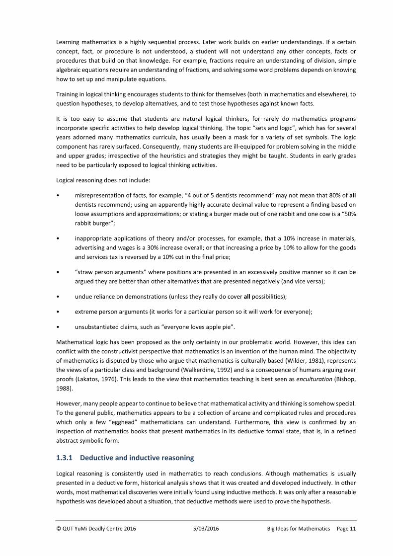
Logical reasoning is consistently used in mathematics to reach conclusions. Although mathematics is usually presented in a deductive form, historical analysis shows that it was created and developed inductively. In other words, most mathematical discoveries were initially found using inductive methods. It was only after a reasonable hypothesis was developed about a situation, that deductive methods were used to prove the hypothesis.
Page 12 Global Big Ideas 5/03/2016 © QUT YuMi Deadly Centre 2016
Inductive reasoning starts with specific examples or observations to identify the underlying rules or patterns, similar to what a scientist or detective does. Whilst inductive reasoning is based on what is observed in the real world, it is never completely certain, because the next observation might contradict the conclusion, or require that it is modified. That is why some scientific ideas (theories) have changed over the years as new information leads to a review of earlier thinking.
Deductive reasoning commences with basic mathematical rules that apply to situation, called axioms (such as the commutative principle for addition), and applies logic to those rules to prove that another, more complex, fact is true. This is what occurs in many areas of mathematics. Deductive reasoning results in certainty – as long as the original rules are valid. This deductive process is unique to mathematics. It is what has given mathematics its stength, and has ensured that mathematical ideas (theorems) do not need to be discarded as new information becomes available.
To summarise visually:
INDUCTION DEDUCTION
Gather information Develop axioms/propositions
Organise/observe patterns Apply rules of logic
Form conclusion/generalisation Prove result (“theorem”)
1.3.2 Mathematical proof
In mathematics, a proof is a logical argument that shows that is a mathematical statement is true. The argument may draw on self-evident axioms (for example, that 2 + [4 + 5] = [2 + 4] + 5), or statements that have previously established using deductive methods, known as theorems. A proof must use methods that show that the proposition is true in every possible circumstance because a single example is all that is needed to disprove a proposition. Sometimes a statement follows from a previously proven proposition with little or no additional work; such a statement is called a corollary. Mathematicians often use the term elegant to describe a proof that is clear and concise.
Whilst the study of proofs has become less common in junior school mathematics in the past century, it is important that they understand that almost all mathematical thinking is underpinned by ideas that can be proved. Students should experience some simple deductive proofs, when appropriate, even if they are not required to develop the proof for themselves. Proofs become more important in the senior secondary years, when students may explore proofs using deduction, induction and contradiction.
Inductive arguments relying only on examples, no matter how many of them there are (called demonstrations), are not accepted as proof. An exception applies if it is possible to show that every possible example is true (a method, jokingly called proof by exhaustion, that is becoming more common now that computers can be programmed to test every possibility). A proposition that has not yet been proven is called a conjecture.
1.3.3 Boolean operators and conditional statements
The words and, or and not have precise meanings in mathematics and logic and are known as logical or Boolean operators. The word and is used to connect two statements and means that both must statements must be true simultaneously, for example the student is a girl and the student has brown eyes refers only to girls with brown eyes. The word or when used to connect two statements means that one or other, or both statements must be true, for example the student is a girl or the student has brown eyes refers to all girls and also those boys with brown
© QUT YuMi Deadly Centre 2016 5/03/2016 Big Ideas for Mathematics Page 13
eyes. Finally, the word not is used to refer to the opposite or complement, for example the student is not a girl refers to boys. Venn diagrams are often used to assist in the interpretation of statements that use combinations of and, or and not.
A conditional statement is in two or more parts formed by combining facts using words such as if ... then or if … then …or else… or if and only if. For example, if a quadrilateral is a square then all the angles are right angles. A conditional statement can also be called an implication and is represented by the symbols ⇒ or →, for example p ⇒ q is read as “if p is true then q is true”.
Some conditional statements are true in one direction only. In the above example, “if a quadrilateral is a square then all the angles are right angles” is true, but the reverse “if all the angles in a quadrilateral are right angles then it is a square” is not true, since the quadrilateral could also be a rectangle. This is called a sufficient condition, since knowing that the shape is a square is sufficient to be certain that the angles are right angles. Going the other way, knowing that the angles are right angles is necessary (but not sufficient) for the shape to be a square.
A statement that is true in both directions is represented by the words if and only if and the symbols ⟺ or ⟷, for example, “two straight lines are perpendicular if and only if they interest at right angles” means that “if two straight lines are perpendicular then they intersect at right angles” and also that “if two straight lines intersect at right angles then they are perpendicular”. Statements that go both ways are called necessary and sufficient.
In addition to their use in mathematics, Boolean operators and conditional statements are commonly used in computer programming (a discipline that builds on the logical reasoning first developed in mathematics). For example, and, or and not are used to connect and define the relationships between search terms entered into an internet search engine.
1.4 Language
An important function of mathematics is language; that is, mathematics is considered as a powerful succinct language for describing relationships and change. Thinking of mathematics as a language changes the way mathematics is taught. Time should be spent on developing meaning for words and symbols, and in translating from real-world situations to mathematical language and vice versa. These ideas are developed further in section the Supplementary Resource 3 about Literacy.
1.4.1 Diverse representations
Mathematical ideas are represented in many ways: words (with some words having different or more precise meanings when used mathematically), symbols, tables and visual images (for example, graphs and diagrams). The language of mathematics can be used to describe the world succinctly and in a generalised way. For example, 2 + 3 could mean that 2 fish were caught and then another 3 fish were caught, or a $2 chocolate and a $3 drink were purchased, or a 2m length of wood was joined to a 3m length ... and so on. The symbols 2 + 3 do not change, but the surrounding words do. Alternatively, 2 + 3 could be represented in the column of a table, with the total of 5 at the foot of the column, or visually on a number line.
This means that mathematical teaching and learning involves continual interchange between different forms of communication and the stories they represent, between formal mathematics and the world.
It is important to see mathematics as a succinct language that describes everyday life as well as a structure of sequenced and connected knowledge. Students should be able to recall and structure their mathematical ideas using many different representations so that they can make a seamless transition between words, symbols, tables and visual images.
Page 14 Global Big Ideas 5/03/2016 © QUT YuMi Deadly Centre 2016
1.4.2 Notion of unit
Anything can be a unit: a single object, a collection of objects, a part of the object (after it has been cut into pieces). Units can form groups and units can be partitioned into parts. For example, if there are six counters, each counter can be a unit, making six units, or the set of six can be a unit, making one unit, or the counters could all be cut into quarters and each quarter could be a unit. This means that mathematics can be perceived very flexibly. For example, eight counters can be considered as eight, one or 50%, depending on need; and 248 can be considered as 248 ones, 24.8 tens, 2.48 hundreds, or 24,800%.
1.4.3 Exactness, accuracy and precision vs estimation and approximation
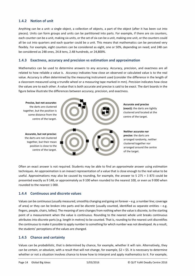
Mathematics can be used to determine answers to any accuracy. Accuracy, precision, and exactness are all related to how reliable a value is. Accuracy indicates how close an observed or calculated value is to the real value. Accuracy is often determined by the measuring instrument used (consider the difference in the length of a classroom measured using a trundle wheel or a measuring tape marked in mm). Precision indicates how close the values are to each other. A value that is both accurate and precise is said to be exact. The dart boards in the figure below illustrate the differences between accuracy, precision, and exactness.
Often an exact answer is not required. Students may be able to find an approximate answer using estimation techniques. An approximation is an inexact representation of a value that is close enough to the real value to be useful. Approximations may also be caused by rounding, for example, the answer to 5 275 + 3 873 could be presented exactly as 9 148, or approximately as 9 100 when rounded to the nearest 100, or even as 9 000 when rounded to the nearest 1 000.
1.4.4 Continuous and discrete values
Values can be continuous (usually measured, smoothly changing and going on forever – e.g. a number line; coverage of area) or they can be broken into parts and be discrete (usually counted, identified as separate entities – e.g. fingers, people, chairs, lollies). The meaning of zero changes from nothing when the value is discrete, to the starting point of a measurement when the value is continuous. Rounding to the nearest whole unit breaks continuous attributes into discrete parts (e.g. length in metres) to be counted. That is, rounding to the nearest unit discretifies the continuous to make it possible to apply number to something for which number was not developed. As a result, the students’ perceptions of the values are changed.
1.4.5 Chance and certainty
Values can be probabilistic, that is determined by chance, for example, whether it will rain. Alternatively, they can be certain, or absolute, with a result that will not change, for example, $2 + $5. It is necessary to determine whether or not a situation involves chance to know how to interpret and apply mathematics to it. For example,
Accurate, but not precise: the darts are not clustered
together, but their mean position is close to the
centre of the target.
Precise, but not accurate: the darts are clustered
together, but the position is some distance from the
centre of the target.
Accurate and precise (exact): the darts are tightly clustered and located at the centre of the target.
Neither accurate nor precise: the darts are arranged randomly, neither clustered together nor arranged around the centre of the target.
© QUT YuMi Deadly Centre 2016 5/03/2016 Big Ideas for Mathematics Page 15
a student’s test result is probabilistic (uncertain) because the set of questions in the test are a sample of the large number of questions that could have been asked – a test conducted on the next day using a different set of questions may yield different results. The use of probability is increasing as large data sets and inference increase in importance.
1.5 Problem solving
1.5.1 Creative and routine problems
The continuum of problems is from creative, that is, they have no particular domain of knowledge, to routine, meaning that they have a specific domain of knowledge – e.g. algebra, fractions, word problems (note that in context the meaning of routine is different from its use in other contexts). The ability to solve creative problems is based on metacognition, thinking skills, plans of attack, strategies, and affects, while the ability to solve routine problems is based on knowledge – the extent that the knowledge is rich (defined, connected, inclusive of applications, and experiences remembered) with basics automated.
1.5.2 Finding, solving and reporting
There are three steps in problem solving: (a) finding –the ability to find and define a problem for later solution (also called problem posing); (b) solving – the ability to use knowledge, strategies, and so on, to come up with a solution; and (c) reporting – writing a neat, well-argued case for their solution. It should be noted that these three steps should not be confused and integrated. For example, solving is a very messy doodling and drawing type activity, while reporting is neat and well set out.
1.5.3 Cognitive processes and affects
The basic processes of good problem solving are: (a) metacognition – awareness and control of one’s own thinking; and (b) thinking skills – logical, visual, creative, flexible and decision making. These higher cognitive processes can be enabled through a plan of attack and problem-solving strategies (see section …).
Studies of expertise in problem situations for which there is a domain of knowledge (e.g. medicine, chess, ballet, mathematics) have shown that it is based on having: (a) knowledge of ideas in a structure that defines, connects and applies in relation to remembered experience of the ideas; and (b) the basics of the expertise automated (memorised) so that they can be recalled without extra cognitive load. Therefore, powerful knowledge is based on consolidation, practising ideas to familiarity, connecting them to other ideas, and memorising the important foundational skills.
Expertise in mathematics also depends on strong affects, in particular, motivation and interest, resilience and persistence, self-confidence, and positive attribution.
YDM Supplementary Book 2 examines Problem Solving in more detail.

© QUT YuMi Deadly Centre 2016 5/03/2016 Big Ideas for Mathematics Page 17
2 Concept Big Ideas
This section looks at the eleven conceptual big ideas of YDM. They are: infiniteness; numeration; attributes; equality; addition and subtraction; multiplication and division; patterns and functions; rates; transformations; shapes; and statistics and probability.
2.1 Numeration
2.1.1 Counting numbers
Numeration is one of the first mathematical concepts to be introduced at school and continues to be developed in various forms throughout the thirteen years of schooling. Understanding number requires the integration of the following concepts, each of which is an integration of sub-concepts: counting, place value, seriation, and renaming.
Counting
Counting requires integration of the following concepts: (a) being able to say the numbers in correct order (rote counting); (b) knowing that each number name is assigned to one and one only object (one-to-one correspondence); (c) imagining a path through the objects that passes through each object once (visualising); (d) being able to continuously separate those that have been counted from those that are yet to be counted; (e) knowing that the last number name said gives the number of objects (rational counting); (f) knowing that any order of counting will give the same answer (trusting the count); and (g) knowing that any set of discrete objects (even imaginary) can be counted.
Place value
Place value is the basis of number systems where the full value of digits is determined by their position as well as their digit or face value. Positional or place value is built around powers of a base number. For the Hindu-Arabic system the base is 10 so that the positions move left and right from 1 (or 100) with positive or negative numbers as follows.
Thousand Hundred Ten One Tenth Hundredth Thousandth
103 102 101 100 10-1 10-2 10-3
Thus, for example, in 4 567.89, the 4 is 4 thousand, the 5 is 5 hundred, the 6 is sixty, the 7 is just seven, the 8 is 8 tenths, and the 9 is 9 hundredths.
Seriation
Seriation is the understanding to add or subtract one of a place value from a number. For example, for 325.697, adding a ten is 335.697 and subtracting a hundredth is 325.687. It also applies to mixed numbers, for example, for 34/6 add one more sixth is 35/6, and 5 subtract 1/5 is 44/5.
Renaming
Renaming is understanding that there are multiple ways of considering a number in terms of place-value positions. For example, if H is hundreds, T is tens, O is ones, t is tenths and h hundredths, then;
345.67 = 3H 4T 5O 6t 7h = 34T 5O 67h = 2H 13T 15O 4t 27h = 11T 232O 14t 227h
It also applies to mixed numbers in that 42/7 = 39/7 = 30/7 (e.g. mixed numbers to improper fractions).
Page 18 Concept Big Ideas 5/03/2016 © QUT YuMi Deadly Centre 2016
Comparison/Order
Order is understanding that, for two numbers, one can be larger/smaller than the other (comparison) and, for more than two numbers, the numbers can be placed in ascending or descending order (ordering).
2.1.2 Fractional equivalence
Equivalence is understanding that two numbers represented in different ways (that is, with different numerals) can be the same value; for example, 0046 = 46, 3.70 = 3.7, and 3/4 = 6/8 = 9/12 and so on. It also applies to different notational forms that give the same value, for example 3/4 = 75% = 0.75.
2.1.3 Multiplicative comparison
Multiplicative comparison arises in the big idea of multiplication and division, but it is also a relationship between two numbers that defines three representations of a number:
(a) percent – 54% is a relation between a number (in this example, 54) and 100, and can also be represented as 54/100, 0.54;
(b) rate – $3.56 per kg is a relationship between mass and price where, in this example, mass is multiplied by 3.56 to give dollars; and
(c) ratio – cordial to water is 2 : 9, which means that the amount of cordial is multiplied by 9 ÷ 2 = 4.5 to get the amount of water.
2.1.4 Other representations of number
Once the counting numbers (also known as natural numbers) are well understood, the big idea of numeration can be extended to accommodate:
• whole numbers (the counting numbers with the inclusion of zero); • integers (the positive whole numbers and zero joined with the negative whole numbers); • rational numbers (bringing in fractions, both common and decimal); • scientific/standard notation, for example 3.23 x 10⁴ or 6.723 x 10⁻⁷ • irrational numbers including surds such as √2 and transcendental numbers such as π; • real numbers, made up of rational and irrational numbers; • imaginary and complex numbers, based on i, where i2 = -1 (or 𝑖𝑖 = √−1);
• matrices, which have elements arranged in rows and columns, for example �2 −35 0 �,
• logarithms, where 43 = 64 can be represented as log464 = 3; and • numbers to other bases, for example where 215 (base 10) can be represented as 11010111 (binary
form), 327 (octal form) and D7 (hexadecimal form).
2.1.5 Algebra
Algebra can be viewed as a generalisation, or abstraction, of the work done in number. Abstraction is a process by which a generality is determined from particular examples. The use of number is, of itself, an abstraction. By experiencing, for instance, many examples of two items (e.g. 2 eyes, 2 hands, 2 chairs, 2 children, and so on), students generalise the language “two” and the symbol “2” as representing the “twoness” that is common to those examples. In a similar way, students gradually build understanding of the language and symbols of all numbers.
When numbers and their names and symbols are new to students, meaning lies with the things or items being counted. However, with experience, it becomes less important to think of items when we use numbers. After a while, 2 + 3 can be considered as equal to 5 without having to think of 2, 3 and 5 as specific items. The thinking simply relates to the symbols 2, 3 and 5. That is, the numbers become the focus or “objects” of thought; not the
© QUT YuMi Deadly Centre 2016 5/03/2016 Big Ideas for Mathematics Page 19
items that underlie them. At this point, the activity with real-world items has been abstracted to numbers and arithmetic.
However, abstraction does not stop with number. After a further time, students start to see that sometimes things are the same regardless of the size and type of the numbers. An example of this is the commutative principle, which says that for any number, addition is the same regardless of the order in which numbers are added (e.g. 2 + 3 = 3 + 2; 656 + 172 = 172 + 656; 31/4 + 22/5 = 22/5 + 31/4, and so on). For this principle, letters such as x and y can be introduced as symbols for variables (i.e. to stand for “any number”) and used to represent the principle, that is, x + y = y + x. As they progress, students may also note that the commutative principle also holds for multiplication and can be extended to more than two numbers and to algebra.
As with numbers, when variables and their names and symbols (letters) are new to students, meaning lies with the numbers that the variables could represent. For example, 2x + 3 is thought of as two multiplied by “any number” plus 3. Solving 2x + 3 = 11 means thinking like “I have a number, I multiply it by two, add 3 and end up at 11; to solve it, I subtract the 3 from 11 (get 8) and divide the 8 by 2 (get 4), so x = 4”. The focus of thinking is on the numbers. However, over time as more experience is gained, it becomes less necessary to think of variables as numbers. The thinking simply focuses on the letters (e.g. 2x + 3x = 5x without thinking of x as a number). thus, the variables become the focus or the “object” of thought. At this point, the numbers and arithmetic have been abstracted to variables and algebra. Overall, what this means is that the development from the real-world items to variables and algebra involves two steps: abstraction from items to numbers; and abstraction from numbers to variables and algebra. That is, algebra is an abstraction of an abstraction.
As students extend their numeration concepts to algebra, they must appreciate that algebra is a form of shorthand that leaves out unnecessary information, for example, xy = x × y. There is no ambiguity in this situation because we understand that a variable represents a number of unknown size, not a numeral so, although x = 2 and y = 3, xy does not mean 23. This leads to important differences between the notation of number and notation of algebra. These ideas can be developed in the context of substituting values into an expression.
However, in the early years, algebra is not about 𝑥𝑥’s and 𝑦𝑦’s; it is about doing and understanding number (and arithmetic) in a deeper way that builds structure and prepares students for algebra. As students’ mathematical understanding progresses the emphasis changes to understanding the world algebraically, manipulating equations and expressions, solving equations, and expressing and representing functions.
Interestingly, the process of abstraction involves gain and loss. Power is gained – we end up with knowledge that is much more portable and can be used in many situations. However, the links back to reality (meaning) are lost – the knowledge is highly symbolic and relationship back to the items it initially came from becomes more difficult.
2.1.6 Measurement
Number and measurement have strong connections. They are seen by YDM as aspects of the same big idea.
Whole and decimal numbers are built around a “pattern of threes” macrostructure (... billions, millions, thousands, ones, thousandths ...) with a sub-pattern or microstructure of hundreds, tens and ones. This same pattern is observed in metric measurement where, for example: if thousandths are millimetres, ones are metres and thousands are kilometres; or if ones are millimetres, thousands are metres and millions are kilometres. In this way, the metric system shares the structure of decimal number. Movements from thousandths → ones → thousands → millions involves multiplying by 1000, as does mm → m → km. Similarly, millions → thousands → ones → thousandths requires division by 1000, just like the movement from km → m → mm. Whilst these examples relate to the units of length, similar patterns occur in units of mass (mg/g/kg/tonne), capacity (mL/L/kL/ML/GL) and energy/work (joules/kilojoules).
Fractions (and division) divide a whole into equal pieces. Similarly, units of measurement divide a length into equal sections (e.g. metres or hand span). Thus, units of measurement share the same inverse relation with
Page 20 Concept Big Ideas 5/03/2016 © QUT YuMi Deadly Centre 2016
fractions: the smaller the denominator, the larger the fraction, and the smaller the unit, the larger the number of units.
The relation between number and measurement is not the only connection between measurement and other branches of mathematics. There are important connections to some of the other conceptual big ideas, including multiplication and division, and shapes, which must also be addressed. However, YDM argues that a pedagogy that links measurement to the underlying big ideas is more powerful in developing understanding than one that treats measurement as a stand-alone topic.
2.2 Equality
2.2.1 Equals as same value
Equality represents the idea that quantities, or expressions, have the same value. Equality is represented by the symbol =.
Congruence is a closely related idea that applies in geometry. Two objects are said to be congruent if one can be exactly superimposed on the other. Congruence is a broader idea than equality because it applies to shape and size, whilst equality applies only to size. Congruence deals with objects (usually geometric figures) while equality deals with numbers. We do not say that two shapes are equal, nor that two numbers are congruent. Congruence is represented by the symbol ≡.
2.2.2 Equivalence and equations
Any number sentence with two expressions connected by an equals sign is called an equation, for example 3 + 5 = 9. However, the word equation is probably more commonly associated with algebraic applications, for example 3x + 5 = 9
Students often see the equals sign as meaning “the answer is written next”. This kind of thinking leads to common, but illogical strings such as: 3x + 2 = 8 – 2 = 6 ÷ 3 = 2. Whilst it may explain a student’s thinking in solving the equation, it is an unacceptable use of notation, for example it includes the incorrect statement 8 – 2 = 6 ÷ 3. The problem is solved by separating each step onto a new line:
3𝑥𝑥 + 2 = 8 3𝑥𝑥 = 8 − 2 3𝑥𝑥 = 6 𝑥𝑥 = 6
3� 𝑥𝑥 = 2
In this presentation, the statements on each line are true (assuming that the first line is true), that is, the expressions on both sides of the equals sign have the same value.
This example illustrates why it is important that teachers understand the future development of a big idea and what can go wrong if early misconceptions are not addressed. Teachers can pre-empt this problem (that is, prepare for the mathematics to be taught in later years) by emphasising that equals means “same value as”, not “write the answer here”. One way of doing this is to regularly present equations with the simplified form on either side of the equation, for example: 2 + 3 = 5 and 5 = 2 + 3; or 4 × 5 = 20 and 20 = 4 × 5.
2.2.3 Comparisons
Equality is a form of mathematical comparison, arising when two mathematical objects have the same value. The big idea of equality can be extended to other forms of mathematical comparison between two values, using the symbols shown below.
© QUT YuMi Deadly Centre 2016 5/03/2016 Big Ideas for Mathematics Page 21
Equality = Equal to ≡ Equivalent to, congruent to ≈, ≑ Approximately equal to
Inequality <, > Less than, greater than ≤, ≥ Less than or equal to, greater than or equal to ≪, ≫ Much less than, much greater than ≠ Not equal to (a line through any comparison symbol has the effect of adding the word “not”)
Other ∝ Proportional to
2.2.4 Various meanings of equality
As students develop mathematically, they may come to see that the meaning of equals has subtle differences, depending on the context (that is why computer programmers distinguish between =, == and ===).
• Simplification: “2 + 3 = 5” really means “2 + 3 can be simplified to 5”. The equals sign is used as a transition from a complex form on the left to an equivalent, simpler form on the right.
• Temporary assignment: a statement such as “speed = 80” means “in this situation, the speed is 80”. It applies only to the problem at hand.
• Definition/identity: for a mathematical truth such a2 – b2 = (a + b)(a – b), the equals sign means “must always be equal to” or “can be seen as” or “is identical to” because it describes a relationship or identity that applies in every situation, not just for particular values. In these cases, the symbol ≡ can also be used, meaning “is equivalent to” [in addition to the meaning “is congruent to” discussed earlier].
• Constraints: we can view the simultaneous equations x + 3y = 5 and x – y = 1 as conditions we want to be true, that is “x + 3y should be 5, if possible” and “x – y should be 1, if possible”. In this case we can satisfy both constraints (x = 2 and y = 1). However, in other situations we cannot meet both constraints (for example, x + 3y = 5 and x + 3y = 1); then the equations might be true individually but not together.
2.3 Addition and subtraction
Addition, and the inverse subtraction, underpins almost all aspects of mathematics. Whilst it may be tempting to think of all the operations (addition, subtraction, multiplication and division) as a single big idea, the similarities outlined in this section explain why YDM treats addition and subtraction as a big idea separate from multiplication and division.
2.3.1 Meaning of addition
Addition and subtraction each have four meanings:
• Joining/separating – this is the basic actions of the two operations, addition as joining and subtraction as take away (e.g. 3 cats join 4 cats; 7 cats and 2 leave).
• Part-part-total – addition involves knowing the parts and finding the total; subtraction is knowing the total and one part and finding the other part. This model covers all addition and subtraction problem types. It includes inaction, where supersets or subsets are formed (e.g. 3 cats and 4 dogs, how many animals?; 7 animals, 5 are dogs, how many cats?).
• Comparison and change – this is where there are two sets and want to find one of the sets or the difference between the sets (e.g. John had 4 cats, Jenny has 3 more cats than the John, how many cats
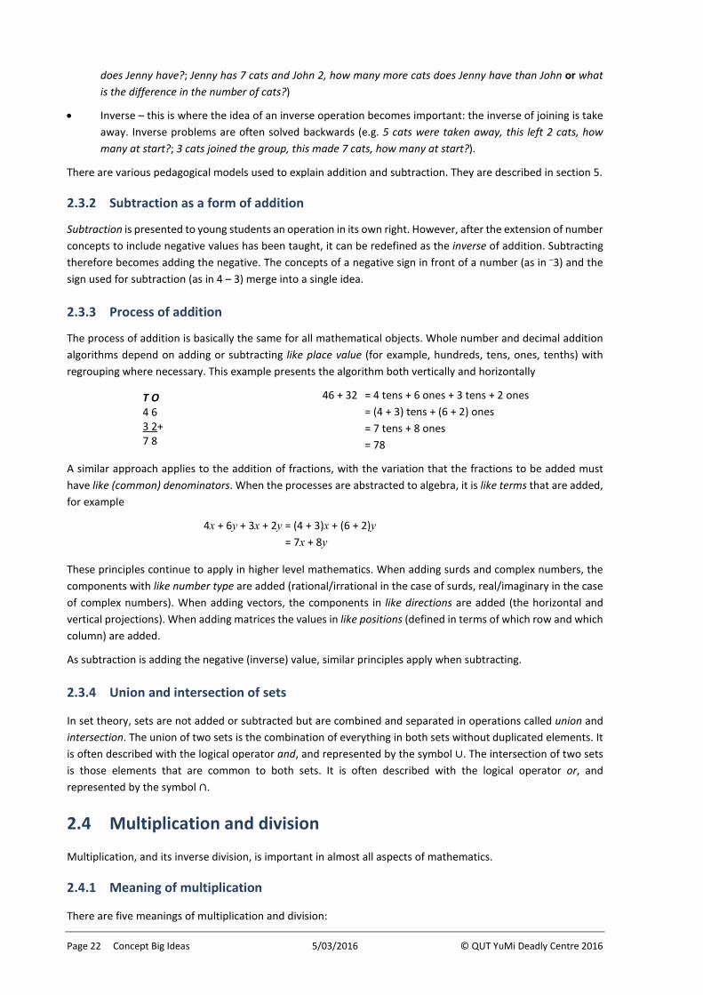
Page 22 Concept Big Ideas 5/03/2016 © QUT YuMi Deadly Centre 2016
does Jenny have?; Jenny has 7 cats and John 2, how many more cats does Jenny have than John or what is the difference in the number of cats?)
• Inverse – this is where the idea of an inverse operation becomes important: the inverse of joining is take away. Inverse problems are often solved backwards (e.g. 5 cats were taken away, this left 2 cats, how many at start?; 3 cats joined the group, this made 7 cats, how many at start?).
There are various pedagogical models used to explain addition and subtraction. They are described in section 5.
2.3.2 Subtraction as a form of addition
Subtraction is presented to young students an operation in its own right. However, after the extension of number concepts to include negative values has been taught, it can be redefined as the inverse of addition. Subtracting therefore becomes adding the negative. The concepts of a negative sign in front of a number (as in –3) and the sign used for subtraction (as in 4 – 3) merge into a single idea.
2.3.3 Process of addition
The process of addition is basically the same for all mathematical objects. Whole number and decimal addition algorithms depend on adding or subtracting like place value (for example, hundreds, tens, ones, tenths) with regrouping where necessary. This example presents the algorithm both vertically and horizontally
46 + 32 = 4 tens + 6 ones + 3 tens + 2 ones = (4 + 3) tens + (6 + 2) ones = 7 tens + 8 ones = 78
A similar approach applies to the addition of fractions, with the variation that the fractions to be added must have like (common) denominators. When the processes are abstracted to algebra, it is like terms that are added, for example
4x + 6y + 3x + 2y = (4 + 3)x + (6 + 2)y = 7x + 8y
These principles continue to apply in higher level mathematics. When adding surds and complex numbers, the components with like number type are added (rational/irrational in the case of surds, real/imaginary in the case of complex numbers). When adding vectors, the components in like directions are added (the horizontal and vertical projections). When adding matrices the values in like positions (defined in terms of which row and which column) are added.
As subtraction is adding the negative (inverse) value, similar principles apply when subtracting.
2.3.4 Union and intersection of sets
In set theory, sets are not added or subtracted but are combined and separated in operations called union and intersection. The union of two sets is the combination of everything in both sets without duplicated elements. It is often described with the logical operator and, and represented by the symbol ∪. The intersection of two sets is those elements that are common to both sets. It is often described with the logical operator or, and represented by the symbol ∩.
2.4 Multiplication and division
Multiplication, and its inverse division, is important in almost all aspects of mathematics.
2.4.1 Meaning of multiplication
There are five meanings of multiplication and division:
T O 4 6 3 2+ 7 8
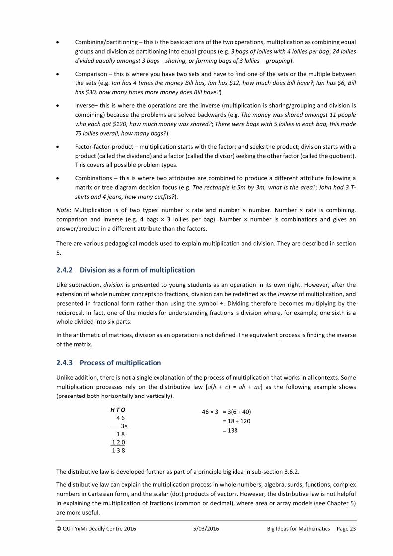
© QUT YuMi Deadly Centre 2016 5/03/2016 Big Ideas for Mathematics Page 23
• Combining/partitioning – this is the basic actions of the two operations, multiplication as combining equal groups and division as partitioning into equal groups (e.g. 3 bags of lollies with 4 lollies per bag; 24 lollies divided equally amongst 3 bags – sharing, or forming bags of 3 lollies – grouping).
• Comparison – this is where you have two sets and have to find one of the sets or the multiple between the sets (e.g. Ian has 4 times the money Bill has, Ian has $12, how much does Bill have?; Ian has $6, Bill has $30, how many times more money does Bill have?)
• Inverse– this is where the operations are the inverse (multiplication is sharing/grouping and division is combining) because the problems are solved backwards (e.g. The money was shared amongst 11 people who each got $120, how much money was shared?; There were bags with 5 lollies in each bag, this made 75 lollies overall, how many bags?).
• Factor-factor-product – multiplication starts with the factors and seeks the product; division starts with a product (called the dividend) and a factor (called the divisor) seeking the other factor (called the quotient). This covers all possible problem types.
• Combinations – this is where two attributes are combined to produce a different attribute following a matrix or tree diagram decision focus (e.g. The rectangle is 5m by 3m, what is the area?; John had 3 T-shirts and 4 jeans, how many outfits?).
Note: Multiplication is of two types: number × rate and number × number. Number × rate is combining, comparison and inverse (e.g. 4 bags × 3 lollies per bag). Number × number is combinations and gives an answer/product in a different attribute than the factors.
There are various pedagogical models used to explain multiplication and division. They are described in section 5.
2.4.2 Division as a form of multiplication
Like subtraction, division is presented to young students as an operation in its own right. However, after the extension of whole number concepts to fractions, division can be redefined as the inverse of multiplication, and presented in fractional form rather than using the symbol ÷. Dividing therefore becomes multiplying by the reciprocal. In fact, one of the models for understanding fractions is division where, for example, one sixth is a whole divided into six parts.
In the arithmetic of matrices, division as an operation is not defined. The equivalent process is finding the inverse of the matrix.
2.4.3 Process of multiplication
Unlike addition, there is not a single explanation of the process of multiplication that works in all contexts. Some multiplication processes rely on the distributive law [a(b + c) = ab + ac] as the following example shows (presented both horizontally and vertically).
46 × 3 = 3(6 + 40) = 18 + 120 = 138
The distributive law is developed further as part of a principle big idea in sub-section 3.6.2.
The distributive law can explain the multiplication process in whole numbers, algebra, surds, functions, complex numbers in Cartesian form, and the scalar (dot) products of vectors. However, the distributive law is not helpful in explaining the multiplication of fractions (common or decimal), where area or array models (see Chapter 5) are more useful.
H T O 4 6 3× 1 8 1 2 0 1 3 8
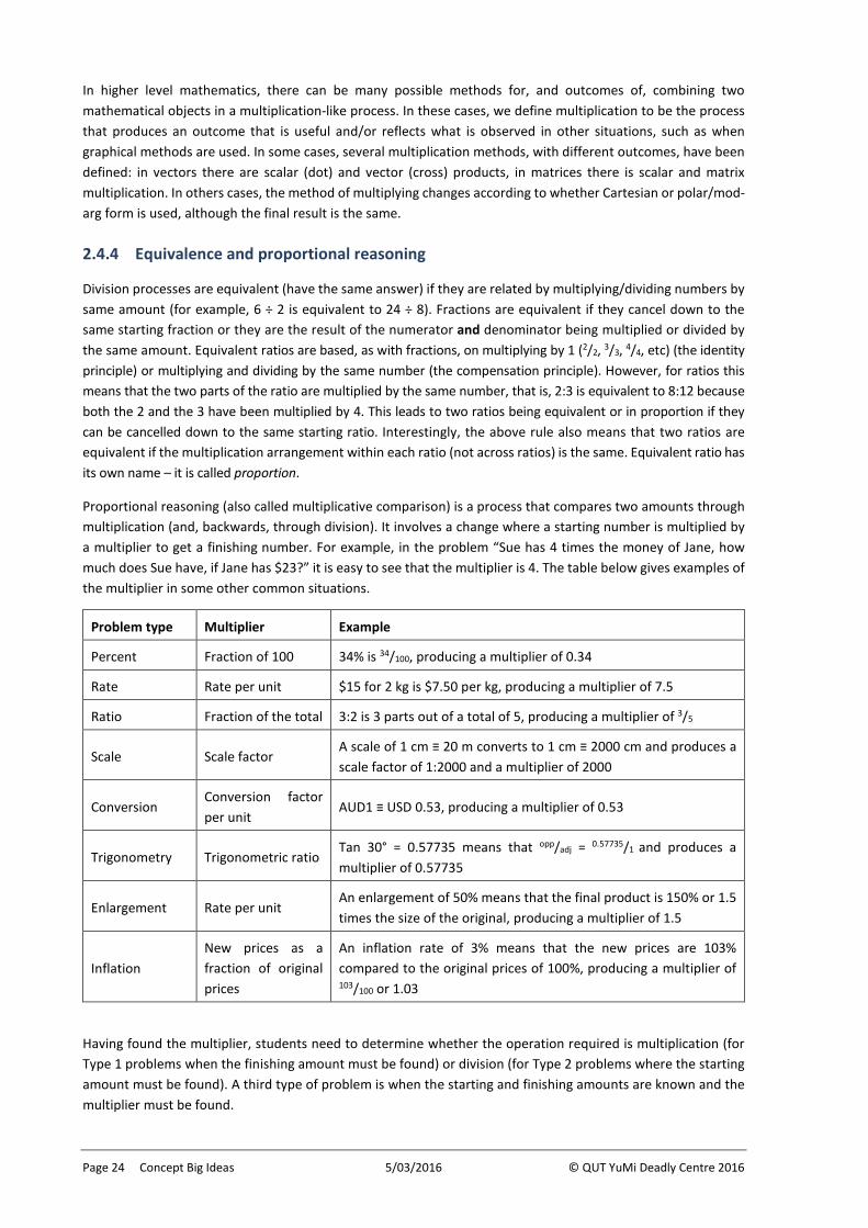
Page 24 Concept Big Ideas 5/03/2016 © QUT YuMi Deadly Centre 2016
In higher level mathematics, there can be many possible methods for, and outcomes of, combining two mathematical objects in a multiplication-like process. In these cases, we define multiplication to be the process that produces an outcome that is useful and/or reflects what is observed in other situations, such as when graphical methods are used. In some cases, several multiplication methods, with different outcomes, have been defined: in vectors there are scalar (dot) and vector (cross) products, in matrices there is scalar and matrix multiplication. In others cases, the method of multiplying changes according to whether Cartesian or polar/mod-arg form is used, although the final result is the same.
2.4.4 Equivalence and proportional reasoning
Division processes are equivalent (have the same answer) if they are related by multiplying/dividing numbers by same amount (for example, 6 ÷ 2 is equivalent to 24 ÷ 8). Fractions are equivalent if they cancel down to the same starting fraction or they are the result of the numerator and denominator being multiplied or divided by the same amount. Equivalent ratios are based, as with fractions, on multiplying by 1 (2/2, 3/3, 4/4, etc) (the identity principle) or multiplying and dividing by the same number (the compensation principle). However, for ratios this means that the two parts of the ratio are multiplied by the same number, that is, 2:3 is equivalent to 8:12 because both the 2 and the 3 have been multiplied by 4. This leads to two ratios being equivalent or in proportion if they can be cancelled down to the same starting ratio. Interestingly, the above rule also means that two ratios are equivalent if the multiplication arrangement within each ratio (not across ratios) is the same. Equivalent ratio has its own name – it is called proportion.
Proportional reasoning (also called multiplicative comparison) is a process that compares two amounts through multiplication (and, backwards, through division). It involves a change where a starting number is multiplied by a multiplier to get a finishing number. For example, in the problem “Sue has 4 times the money of Jane, how much does Sue have, if Jane has $23?” it is easy to see that the multiplier is 4. The table below gives examples of the multiplier in some other common situations.
Problem type Multiplier Example
Percent Fraction of 100 34% is 34/100, producing a multiplier of 0.34
Rate Rate per unit $15 for 2 kg is $7.50 per kg, producing a multiplier of 7.5
Ratio Fraction of the total 3:2 is 3 parts out of a total of 5, producing a multiplier of 3/5
Scale Scale factor A scale of 1 cm ≡ 20 m converts to 1 cm ≡ 2000 cm and produces a scale factor of 1:2000 and a multiplier of 2000
Conversion Conversion factor per unit
AUD1 ≡ USD 0.53, producing a multiplier of 0.53
Trigonometry Trigonometric ratio Tan 30° = 0.57735 means that opp/adj = 0.57735/1 and produces a multiplier of 0.57735
Enlargement Rate per unit An enlargement of 50% means that the final product is 150% or 1.5 times the size of the original, producing a multiplier of 1.5
Inflation New prices as a fraction of original prices
An inflation rate of 3% means that the new prices are 103% compared to the original prices of 100%, producing a multiplier of 103/100 or 1.03
Having found the multiplier, students need to determine whether the operation required is multiplication (for Type 1 problems when the finishing amount must be found) or division (for Type 2 problems where the starting amount must be found). A third type of problem is when the starting and finishing amounts are known and the multiplier must be found.
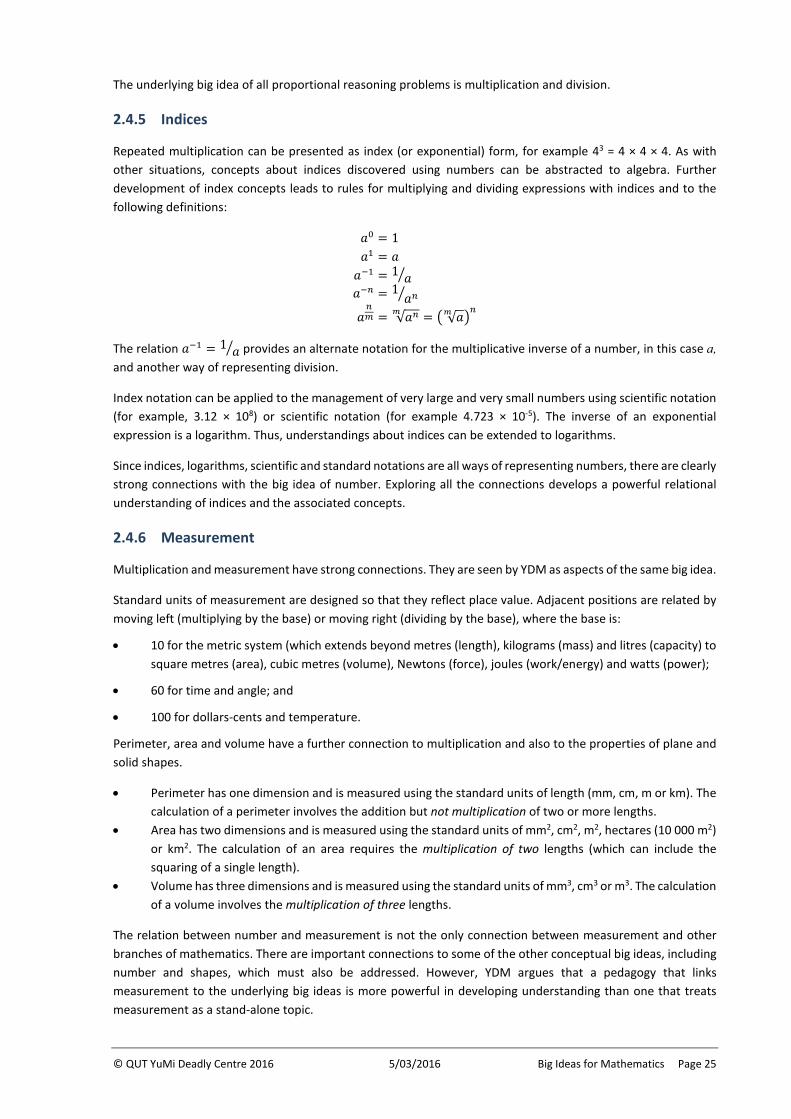
© QUT YuMi Deadly Centre 2016 5/03/2016 Big Ideas for Mathematics Page 25
The underlying big idea of all proportional reasoning problems is multiplication and division.
2.4.5 Indices
Repeated multiplication can be presented as index (or exponential) form, for example 43 = 4 × 4 × 4. As with other situations, concepts about indices discovered using numbers can be abstracted to algebra. Further development of index concepts leads to rules for multiplying and dividing expressions with indices and to the following definitions:
𝑎𝑎0 = 1 𝑎𝑎1 = 𝑎𝑎 𝑎𝑎−1 = 1 𝑎𝑎� 𝑎𝑎−𝑛𝑛 = 1
𝑎𝑎𝑛𝑛�
𝑎𝑎𝑛𝑛𝑚𝑚 = √𝑎𝑎𝑛𝑛𝑚𝑚 = � √𝑎𝑎𝑚𝑚 �
𝑛𝑛
The relation 𝑎𝑎−1 = 1 𝑎𝑎� provides an alternate notation for the multiplicative inverse of a number, in this case a, and another way of representing division.
Index notation can be applied to the management of very large and very small numbers using scientific notation (for example, 3.12 × 10⁸) or scientific notation (for example 4.723 × 10⁻⁵). The inverse of an exponential expression is a logarithm. Thus, understandings about indices can be extended to logarithms.
Since indices, logarithms, scientific and standard notations are all ways of representing numbers, there are clearly strong connections with the big idea of number. Exploring all the connections develops a powerful relational understanding of indices and the associated concepts.
2.4.6 Measurement
Multiplication and measurement have strong connections. They are seen by YDM as aspects of the same big idea.
Standard units of measurement are designed so that they reflect place value. Adjacent positions are related by moving left (multiplying by the base) or moving right (dividing by the base), where the base is:
• 10 for the metric system (which extends beyond metres (length), kilograms (mass) and litres (capacity) to square metres (area), cubic metres (volume), Newtons (force), joules (work/energy) and watts (power);
• 60 for time and angle; and
• 100 for dollars-cents and temperature.
Perimeter, area and volume have a further connection to multiplication and also to the properties of plane and solid shapes.
• Perimeter has one dimension and is measured using the standard units of length (mm, cm, m or km). The calculation of a perimeter involves the addition but not multiplication of two or more lengths.
• Area has two dimensions and is measured using the standard units of mm2, cm2, m2, hectares (10 000 m2) or km2. The calculation of an area requires the multiplication of two lengths (which can include the squaring of a single length).
• Volume has three dimensions and is measured using the standard units of mm3, cm3 or m3. The calculation of a volume involves the multiplication of three lengths.
The relation between number and measurement is not the only connection between measurement and other branches of mathematics. There are important connections to some of the other conceptual big ideas, including number and shapes, which must also be addressed. However, YDM argues that a pedagogy that links measurement to the underlying big ideas is more powerful in developing understanding than one that treats measurement as a stand-alone topic.
Page 26 Concept Big Ideas 5/03/2016 © QUT YuMi Deadly Centre 2016
2.5 Attributes
Objects are defined by their attributes. In mathematics, an attribute is a characteristic or property that applies to a mathematical object. Attributes are described using adjectives, for example red, small, straight, even, skewed.
In the early years students are introduced to attributes using physical objects of various shapes, sizes, colours, and textures. Using these materials, they learn the important skills of classifying and sorting. As they develop mathematically, they learn that attributes can be less tangible and involve mathematical concepts such as parity (odd/even), magnitude, place value, dimension, angle, and units of measurement.
From a mathematical perspective, an attribute is only relevant if it adds worthwhile mathematical information to the discussion or mathematical argument. For example: place value is explicitly identified as an attribute only when it is needed to make sense of a mathematical process; a plus sign is attached to a numeral only when it is required to avoid confusion (that is, for +3 and 3, or to distinguish between 6 + 3 and 63). We could classify the symbols 0, 1, 2, 3, …, 9 as being composed of straight or curved lines, but rarely do so because it is of no worthwhile mathematical use.
2.5.1 One attribute
Rational numbers are generally considered to have one attribute, namely value, also called size or magnitude. However, for some purposes they can be classified into sub-sets such as positive/negative, denominator/numerator, units/tens/hundreds. The rational numbers are comprehensively dealt with as part of the big idea of number.
2.5.2 Two or more attributes
Mathematical objects with two or more attributes different from those with one attribute and are the focus of this big idea. Some numbers can have two attributes, for example: irrational numbers (surds) with rational and irrational parts (for example, 3 + √2); and complex numbers that have real and imaginary parts (for example, 4 5i).
Measurements can be considered as having two attributes: the magnitude and the unit of measurement. Geometric figures are commonly classified by dimension (1, 2 or 3), which link to the concepts of perimeter, area and volume. However, they can also be classified according to orientation/angle, size (length/area/volume), symmetry, similarity or congruence.
Two dimensional objects (shapes, graphs, vectors and complex numbers) may have the attributes defined in Cartesian form (horizontally and vertically, or x and y) or Polar form (magnitude and angle, modulo and argument, or r and θ). Three dimensional objects can be defined in terms of three attributes in Cartesian form (width, depth and height, or x, y and z) or Polar form (magnitude, azimuth and altitude or r, θ, and φ).
The significance of attributes as a big idea is that all attributes of an object must be attended to when applying a mathematical process to that object. For example, to convert a length measured in metres to millimetres requires that both the number and the unit of measurement be changed. To obtain a similar plane shape by enlargement or reduction of the original (a transformation called dilation) it is necessary to apply the same enlargement or reduction factor to both the horizontal and vertical attributes of the original.
Further, the methods of dealing with objects with similar attributes are related, as shown in the following examples.
• The methods used to arithmetically manipulate surds and complex numbers are the same. • The ability to use Cartesian coordinates in two dimensions contributes to the understanding of functions,
vectors and complex numbers, and prepares the way for three dimensional Cartesian coordinates.
© QUT YuMi Deadly Centre 2016 5/03/2016 Big Ideas for Mathematics Page 27
• A knowledge of Pythagoras’ theorem and trigonometry in two dimensions contributes to the understanding of two dimensional functions, vectors and complex numbers expressed in polar forms, and prepares the way for three dimensional applications of Pythagoras and trigonometry, and polar forms of three dimensional vectors and functions.
There may be several connections between mathematical objects with two or more attributes and big ideas, for example with addition and subtraction and multiplication and division. All these connections must also be explored. However, YDM argues that a pedagogy that considers mathematical objects in terms of their attributes is a powerful way of developing mathematical understanding.
2.6 Patterns and functions
Whilst the study of patterns is a global big idea in YDM, patterning as a prelude to algebra and functions is also a conceptual big idea. All the big ideas from arithmetic (particularly equality, addition/subtraction, and multiplication/division), are big ideas in algebra because algebra is the generalisation of arithmetic. Any arithmetic concept that can be expressed as a generality can be an algebra concept big idea.
2.6.1 Generalising patterns
The first stage in working with patterns is generalising from particular examples, identifying, describing and determining a general rule for the pattern.
The general rule for a pattern will usually have fixed and changing parts – the fixed part does not change with the progression from one term to the next, whilst the changing (variable) part is different for each term. The general rule can take one of two forms: a sequential (or recursive) rule is a generalisation that describes the change between consecutive terms; whilst a position rule is a generalisation that relates the position of term to the value of the term. Initially students may develop simple generalised rules using guess and check methods. However, higher level mathematics courses usually include some techniques that can be used to generalise in more complex situations. This early patterning work is further developed in later years as the study of sequences (a pattern of numbers) and series (the sum of a pattern of numbers).
A pattern can be generalised using algebraic notation, for example 3x + 2, where 2 is the fixed part and 3x is the variable part. In this case, the letter x (or any other symbol) can represent any number, varying depending on the situation. It is called a pronumeral. As students develop mathematically, they come to see that have subtle differences in meaning, depending on the context:
• The pronumeral may be used to explore what happens as the value is allowed to change, for example in a function or a relation. In this case, the pro-numeral is called a variable. Variables are often represented using the letters x, y, z (at the end of the alphabet) or n or m if an integer.
• The pronumeral may be value(s) that is not known, for example in an equation such as 3x + 2 = 14. In these cases it is called an unknown. The purpose in using the unknown in this context is to solve the equation to find the value(s) that satisfy it.
• The pronumeral may be used when a generalised expression is required, for example in the y-intercept form of a linear function y = mx + c. In this example the pro-numerals m and c are called parameters. If the values of the parameters are subsequently found out, then the values are usually substituted into the expression. Parameters are often represented using letters a, b, c, etc (at the beginning of the alphabet).
2.6.2 Equations
The big ideas involving equality, operations and patterning can be generalised to algebraic equations. Whilst students start with linear equations, the equation solving techniques can be extended to any type of equation. The pedagogical big ideas of balance and backtracking (a part of the principle big idea of inverse) can be visualised as movements and applied to solve problems for unknowns in equations. Whilst backtracking works well with
Page 28 Concept Big Ideas 5/03/2016 © QUT YuMi Deadly Centre 2016
linear equations, it does not work as well with non-linear equations, so it is important that the idea of balance is developed. Links should be made between the solution of an equation and the x-intercept of the underlying function.
Students are usually introduced to simultaneous equations graphically. The graphical approach can be extended to show that solving an individual equation is actually finding the point of intersection between the underlying function and the line y = 0. Solution methods are then extended to algebraic approaches (elimination and substation) and in the senior years to the use of matrices. Inconsistent simultaneous equations (ie: those with no solution) should be explained in graphical terms.
Mathematical technology such as graphing packages, CAS (computer algebra systems), dynamic algebra software, and even some mobile phone apps are also very powerful classroom tools for teaching about equations.
2.6.3 Functions
Generalised patterns that describe changes or relations are called relations. At least two variables are required: one or more independent variables (inputs) and the dependent variable (output). The possible values of the independent variable is called the domain (labelled x on the Cartesian plane) and the possible values of the dependent variable is called the range (labelled y on the Cartesian plane). A relation can be represented in many ways: tables of values; diagram; graph; coordinates; algebraic equation (in Cartesian, parametric, or polar forms); and mapping.
A function is a particular type of relation where there is only one value of the dependent variable for every value of the independent variable. For example, x = 3 is not a function because (3, 0), (3, 1) and (3, 2) are just some of the values that this relation can take, but are sufficient to demonstrate that there are many different values of the dependent variable (0, 1, 2, …) for only one value of the independent variable (3). A variety of models are used to teach about functions, including
• Various operations are defined for functions: they can be added, subtracted, multiplied and divided (linking to those big ideas), and nested (called composite functions). They also have inverse forms (linked to the principle big idea).
• Functions are often classified by type. Those commonly studied at school level include: linear; conic sections (circle, ellipse, parabola and hyperbola), exponential and logarithmic, and trigonometric.
2.6.4 Coordinates and graphs
In the early years, patterns are explored using groups of students (body) and manipulatives such as counters, blocks, and toothpicks (hand) before progressing to diagrammatic representations of those patterns, both literal and as graphs (mind). Changes to patterns can be shown as having two attributes: the changing value of the pattern (often labelled as y or tn) and its position in the sequence (labelled x or n). In the middle years, the Cartesian plane is introduced as a way of representing these patterns, initially focussing only on the first quadrant, but extending to four quadrants after students learn about negative numbers.
The Cartesian plane is a powerful tool for exploring relations and functions and representing algebraic ideas visually. Basic concepts are introduced in the context of plotting points using a combination of the horizontal and vertical distance from the origin (called Cartesian form), joining points to form lines, and using lines to define regions. This can be developed to include the distance between points, the midpoint of two points, the gradient of a line (one of the foundations of the big idea on rates), the x and y intercepts of a line, and the points of intersection between two or more lines. The Cartesian plane can be used as a tool in other big ideas to understand changes to points, lines, vectors and plane shapes.
Mathematical technology such as graphing packages, CAS (computer algebra systems), and dynamic algebra software are powerful classroom tools for teaching about functions and their graphs.
© QUT YuMi Deadly Centre 2016 5/03/2016 Big Ideas for Mathematics Page 29
The ideas developed using the Cartesian plane can be extended to three dimensions, and to the Argand diagram (a way of representing complex numbers visually). An alternative method of plotting points using the distance from the origin in a particular direction (angle) (called polar form) can be developed and applied to two dimensions (as magnitude, r and angle, θ) and three dimensions (as magnitude, r; horizontal angle or azimuth, θ, and vertical angle or altitude, φ). Work with points, lines and regions in polar form can be extended to functions, vectors and complex numbers.
2.7 Shapes
2.7.1 Points, lines and angles
Points identify the location of a mathematical object. They have no dimension (that is, no length, width or thickness) and are usually labelled with upper case letter.
Lines define a continuous path and are usually labelled AB, where A and B are points on the line. Line intervals have length (distance), usually labelled with a lower case letter. Lines may be straight or curved. Straight lines are defined in one dimension only, having length, but not width or thickness. Straight lines sometimes have direction; lines that have length and direction may be called vectors. Two or more straight lines may be classified as parallel, perpendicular, intersecting, concurrent or skew. Curved lines are classified according to type (for example, circle or ellipse). If there is a straight line and a curved line, the straight line may intersect the curve, touch the curve (tangent) or not meet the curve at all.
Angles are defined by the intersection of lines. They are usually labelled ∠ABC where A and C are points on the arms and B is the vertex. The size of an angle is defined as the amount of turn, and is classified as: acute, right, obtuse, straight, reflex, revolution, and more than a full turn. The size of an angle is usually labelled with a lower case Greek or Roman letter. They are measured using degrees (where 360° is a full rotation) or radians (where 2π is a full rotation). Angles may also be represented by gradient (“steepness”), compass direction, compass bearing, angle of elevation, or angle of depression. There are many angle theorems, including: vertically opposite angles, supplementary angles, complementary angles, angles at a point, and angles on parallel lines (alternate, corresponding, co-interior).
2.7.2 Plane (2D) shapes
All plane shapes can be defined in terms of their geometric properties: points (vertices), lines (sides) and angles. Plane shapes have width and height, but no depth. Those commonly studied at school include polygons, particularly triangles and quadrilaterals, and circles. Key issues associated with the study of these plane shapes are listed below.
• Triangles ₋ usually labelled ΔABC where A, B and C are the vertices ₋ sketching and constructing triangles ₋ triangles defined by their line properties are classified as: equilateral, isosceles, scalene ₋ triangles defined by their angle properties are classified as: acute, obtuse, right ₋ angles in triangles: equilateral, base angles of isosceles triangles, exterior angle ₋ area (using grids, as half a square/rectangle, base and perpendicular height, generalisation to
formulas) ₋ Pythogoras’ theorem ₋ application of trigonometry and vectors to triangles
• Quadrilaterals ₋ usually labelled ABCD where A, B, C and D are the vertices ₋ sketching and constructing quadrilaterals ₋ classification: square, rhombus, rectangle, parallelogram, kite, trapezium/trapezoid, other ₋ line properties: side lengths, parallel sides, diagonals (bisect each other or not?)
Page 30 Concept Big Ideas 5/03/2016 © QUT YuMi Deadly Centre 2016
₋ angle properties: angles at vertices, angles at intersection of diagonals ₋ area (using grids, dividing into triangles, generalisation to formulas) ₋ application of vectors to quadrilaterals
• Other polygons ₋ classification: regular/irregular, concave/convex, named according to number of sides ₋ angles: angles in polygons: angle sum (2n -180), sizes of regular polygons ₋ area (dividing into simpler shapes) ₋ application of vectors to polygons
• Circles ₋ parts of circle: points: centre, on circumference; straight lines (radius, diagonal, chord –
major/minor, tangent, secant), curved lines (circumference, arc – major/minor), regions: semicircle, quadrant, sector – major/minor, segment – major/minor
₋ sketching, constructing ₋ circle theorems ₋ incircles, circumcircles, concentric circles ₋ circumference (measuring, generalisation to formula, π) ₋ area (using grids, approximation as a rectangle, generalisation to formula)
2.7.3 Solid (3D) shapes
All solid shapes can be defined in terms of their geometric properties: points (vertices), lines (edges), angles and surfaces (faces). For solids with plane faces, the edges, faces and vertices are linked by Euler’s formula. Solid shapes at school include prisms, pyramids, the Platonic solids and solids with curved surfaces. Key issues associated with the study of these solids are listed below.
• Prisms ₋ definition: congruent (uniform) cross section, base, height, axis perpendicular to base, sketching ₋ named according to the shape of the base ₋ face properties: two polygons (base), remainder of faces rectangular, nets ₋ line properties: straight edge lengths, many parallel edges ₋ surface area (derived from net), volume (using blocks, layers, generalisation to formula V = Ah) ₋ application of 3D vectors to prisms
• Pyramids ₋ definition: similar cross section, base, height, slant height, sketching ₋ named according to the shape of the base ₋ face properties: one polygon (base), remainder of faces triangular, nets ₋ line properties: straight edge lengths, many edges converge to the apex ₋ surface area (derived from net), volume (using blocks, layers, generalisation to formula V = 1/3Ah) ₋ application of 3D vectors to prisms
• Platonic solids ₋ definition: regularity, all angles and edges congruent ₋ types: tetrahedron (4 triangular faces), cube (6 square faces), octahedron (8 triangular faces),
dodecahedron (12 pentagonal faces), icosahedron (20 triangular faces) • Curved solids
₋ sphere: definition, radius, diameter, volume, surface area ₋ cylinder: definition, circular base, uniform cross-section, rectangular curved side, relation to prism,
radius, height, volume (derived from prism), surface area (from net) ₋ cone: definition, circular base, similar cross-section, curved side is a sector, relation to pyramid,
radius, perpendicular height, slant height, volume (derived from pyramid), surface area (from net)
© QUT YuMi Deadly Centre 2016 5/03/2016 Big Ideas for Mathematics Page 31
2.8 Transformations
A geometric transformation is the movement of points, lines, plane (2D) shapes and functions in the Cartesian plane. Before the transformation the point/line/shape/function is called the object. The image is the result after the transformation has been applied to the object.
2.8.1 Geometric transformations
Geometric transformations can be classified into three categories:
• The simplest transformations are reflection in a line (flip), rotation (turn) and translation (slide). They are called Euclidean transformations because the properties of Euclidian geometry (angle, size and straightness) do not change under these transformations.
• Projective transformations include dilation (enlarging and reducing in one or more directions), shear (moving some points in a fixed direction so that, for example, a square becomes a rhombus – think also of what occurs when the axes of a graph do not meet at right angles), and reflection in a curved surface (think about what occurs when light rays meet concave and convex mirrors). These types of transformations relate different shapes (for examples, ellipses and circles or the different types of quadrilaterals) and cause parallel lines that meet at a “vanishing point”. Important applications include the use of perspective in art and technical drawing, and map projections. Projective transformations change length and angle, but not straightness.
• Topological transformations can include all of the above, but introduce the deformations of stretching and bending. Unlike the other types of transformations, they do not have to be applied in a uniform way. They can be likened to what happens when a piece of wet clay is moulded (without making holes, breaking off pieces, or attaching new pieces). In topological transformations, length, angle and straightness can all change.
The principle of Euclidean transformational invariance means that the angles, lengths and areas do not change as a result of a Euclidean transformation. This principle means that the properties of lines, angles and shapes area do not change if the object is rotated or reflected, or moved around the Cartesian plane (other than orientation). It allows the simplification of many geometric, measurement and Cartesian problems.
2.8.2 Symmetries, congruence and similarity
Transformations can be analysed in terms of symmetry, congruence and similarity.
• Line symmetry – a plane shape has line symmetry when the two sides match when folded in half; that is, if the object and image are identical after reflection in at least one axis (called the axis of symmetry).
• Rotational symmetry – a plane shape has rotational symmetry when the object and image are identical after a rotation of less than 360°.
• Congruence – two plane shapes are congruent if angles and lengths are the same (relationship rule); OR when one can be changed to the other by Euclidian transformations (transformational rule). There are four ways of determining if two triangles are congruent.
• Similarity – two plane shapes are similar if angles are the same and lengths are in the same ratio (relationship rule); OR when one can be changed to the other by a uniform dilation (enlargement or reduction) (transformational rule).
2.8.3 Similarity and trigonometry
The long side of a right angled triangle is called the hypotenuse. The other two sides are labelled as adjacent or opposite according to their relationship to a specified acute angle. Because all right angled triangles with an acute
Page 32 Concept Big Ideas 5/03/2016 © QUT YuMi Deadly Centre 2016
angle of a specified size are similar, the ratios between any two of the sides are constant. These ratios, called trigonometric ratios, are:
sin𝜃𝜃 =opposite
hypotenuse
cos 𝜃𝜃 =adjacent
hypotenuse
tan𝜃𝜃 =adjacentopposite
Trigonometric ratios can be used to find the angle size, side lengths, and area of many triangles, including triangles without right angles. They are also the basis of work with vectors in polar form and complex numbers in mod-arg form.
2.8.4 Transformations of functions
Some transformations can be generalised and applied to the equations of functions. The table below gives examples of some transformations applied to a general function 𝑓𝑓(𝑥𝑥).
Change to the function* Transformation
𝑓𝑓(𝑥𝑥) + ℎ Translation by h units in a vertical direction
𝑓𝑓(𝑥𝑥 − ℎ) Translation by h units to the right
ℎ𝑓𝑓(𝑥𝑥) Vertical dilation by h units
𝑓𝑓(ℎ𝑥𝑥) Horizontal dilation by 1/h units
𝑓𝑓(−𝑥𝑥) Reflection in the x-axis
−𝑓𝑓(𝑥𝑥) Reflection in the y-axis
𝑓𝑓−1(𝑥𝑥) (inverse function) Reflection in the line y = x
*Negative values of h will result in the transformation occurring in the opposite direction
Geometric transformations can be further abstracted so that certain matrices can be applied to the object (defined by key points or as a function) to find the image. This eliminates the need to use diagrams or graphs to find the result of a transformation.
2.9 Infiniteness
2.9.1 Infinitely large
Sets are groups of “objects” (mathematical or otherwise). They can be classified as finite or infinite. Finite sets have a limited number of elements (or members), ranging from zero (known as an empty set or void set) to many. For example, the set containing the names of every citizen of Australia on 1 January 2016 is large (approximately 24 million), but still limited – given enough time (or computer power), it would be possible to list all of the names. Many mathematics books define infinite sets as those which are not finite. This definition, whilst true, is not particularly helpful. It is easier to think of an infinite set as one where the number of elements are unlimited. For example, the set of counting numbers is infinite, as it is possible to continue counting without ever reaching the end. For every counting number that exists, we can always find a larger number simply by adding one more. Infinite sets can be classified in several ways.
© QUT YuMi Deadly Centre 2016 5/03/2016 Big Ideas for Mathematics Page 33
Bounded and unbounded
An unbounded infinite set has no upper or lower limit (or both). For example, the set of counting numbers has a lower limit (1), but no upper limit, and the set of integers has no upper or lower limit, so they are both examples of unbounded sets. However, the set of all decimal fractions between zero and one is infinite because we can create more and more decimal fractions by simply increasing the number of decimal places in the fraction, but as it has an upper and lower bound, we say it is a bounded infinite set.
Countable and uncountable
Infinite sets are countable if we can relate them to the set of counting numbers. For example, the correspondence represented in the following table demonstrates that the set {5, 8, 11, 14, 17, 20, 23, …} is countable.
Counting numbers 1 2 3 4 5 6 7 … ↕ ↕ ↕ ↕ ↕ ↕ ↕
Members of infinite set 5 8 11 14 17 20 23 …
An uncountable infinite set cannot be related to the counting numbers. For example, the table below shows that the infinite set of all decimal fractions between zero and one (discussed earlier) can be related directly to the counting numbers if we confine the analysis to the tenths (shown in black below). However, we encounter problems when we add in just some of the fractions with tenths and hundredths (shown below in grey). This problem becomes even worse as we introduce the rest of the hundredths and even more decimal fractions by including the thousandths, ten thousandths and so on (that is, increasing the number of decimal places infinitely). So, it is not possible to show a one-to-one correspondence between the counting numbers and the set of all decimal fractions between zero and one. Therefore this set is uncountable.
Counting numbers 1 ? 2 ? 3 ? 4 ? 5 ? 6 ? 7 ? … ↕ ↕ ↕ ↕ ↕ ↕ ↕ ↕ ↕ ↕ ↕ ↕ ↕ ↕
Members of infinite set
0.1 0.15
0.2 0.25
0.3 0.35
0.4 0.45
0.5 0.55
0.6 0.65
0.7 0.75
…
Infinity
Infinite is an adjective that comes from the Latin ad infinitum. Infinity, the related noun, can be difficult to define. It is the quality or state of endlessness or having no limits in terms of time, space, or other quantity. No number can exceed infinity. Infinity is represented by the symbol ∞. Alternatively, we can represent an infinite sequence by using three dots (called ellipsis, meaning “and so on”), for example 2, 4, 6, 8, …
Infinity is a tricky idea because it is not a number. We can say that a number increases to infinity, or approaches infinity (in symbols, n → ∞), but not that it is equal to infinity. We can show this for the counting numbers by using a proof by contradiction where we start by assuming the proposition is incorrect:
Assume that n is a counting number equal to infinity, so we can say that n = ∞ It follows logically that n + 1 > ∞ But this is contrary to the definition of infinity which says that that no number can exceed infinity. So,
the previous lines cannot be correct. Therefore, our original assumption (that n is a counting number equal to infinity i.e. n = ∞) must be
incorrect. Therefore n ≠ ∞, that is, no counting number can be equal to infinity.
Similar methods can be used to show that the proposition applies to other types of numbers.
Infiniteness is an important concept in both mathematics and science. The examples in this section demonstrate that the number system is infinite, but so are other mathematical objects such as the number line, the Cartesian plane, and the set of different quadrilaterals that exist. In science, the size of the universe is considered to be infinite, as is the number of stars. However, the number of grains of sand on a beach or hairs on your head is finite.
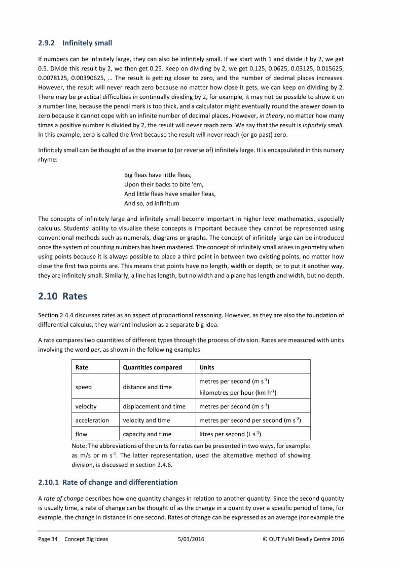
Page 34 Concept Big Ideas 5/03/2016 © QUT YuMi Deadly Centre 2016
2.9.2 Infinitely small
If numbers can be infinitely large, they can also be infinitely small. If we start with 1 and divide it by 2, we get 0.5. Divide this result by 2, we then get 0.25. Keep on dividing by 2, we get 0.125, 0.0625, 0.03125, 0.015625, 0.0078125, 0.00390625, … The result is getting closer to zero, and the number of decimal places increases. However, the result will never reach zero because no matter how close it gets, we can keep on dividing by 2. There may be practical difficulties in continually dividing by 2, for example, it may not be possible to show it on a number line, because the pencil mark is too thick, and a calculator might eventually round the answer down to zero because it cannot cope with an infinite number of decimal places. However, in theory, no matter how many times a positive number is divided by 2, the result will never reach zero. We say that the result is infinitely small. In this example, zero is called the limit because the result will never reach (or go past) zero.
Infinitely small can be thought of as the inverse to (or reverse of) infinitely large. It is encapsulated in this nursery rhyme:
Big fleas have little fleas, Upon their backs to bite 'em, And little fleas have smaller fleas, And so, ad infinitum
The concepts of infinitely large and infinitely small become important in higher level mathematics, especially calculus. Students’ ability to visualise these concepts is important because they cannot be represented using conventional methods such as numerals, diagrams or graphs. The concept of infinitely large can be introduced once the system of counting numbers has been mastered. The concept of infinitely small arises in geometry when using points because it is always possible to place a third point in between two existing points, no matter how close the first two points are. This means that points have no length, width or depth, or to put it another way, they are infinitely small. Similarly, a line has length, but no width and a plane has length and width, but no depth.
2.10 Rates
Section 2.4.4 discusses rates as an aspect of proportional reasoning. However, as they are also the foundation of differential calculus, they warrant inclusion as a separate big idea.
A rate compares two quantities of different types through the process of division. Rates are measured with units involving the word per, as shown in the following examples
Rate Quantities compared Units
speed distance and time metres per second (m s-1)
kilometres per hour (km h-1)
velocity displacement and time metres per second (m s-1)
acceleration velocity and time metres per second per second (m s-2)
flow capacity and time litres per second (L s-1)
Note: The abbreviations of the units for rates can be presented in two ways, for example: as m/s or m s-1. The latter representation, used the alternative method of showing division, is discussed in section 2.4.6.
2.10.1 Rate of change and differentiation
A rate of change describes how one quantity changes in relation to another quantity. Since the second quantity is usually time, a rate of change can be thought of as the change in a quantity over a specific period of time, for example, the change in distance in one second. Rates of change can be expressed as an average (for example the
© QUT YuMi Deadly Centre 2016 5/03/2016 Big Ideas for Mathematics Page 35
average speed during a drive from Brisbane to Sydney) or instantaneous (for example, the speed shown on a car speedometer at a particular moment).
If a graph plots the values of two quantities as a function (curve), for example, the distance travelled by a car at various times during a journey, the average rate of change between two points on the curve is represented graphically by the gradient of the line (secant) joining the two points. The instantaneous rate of change at a particular point on the curve is represented graphically by the gradient of the line (tangent) that touches the curve at that point. By starting with two points, and allowing one point to move closer to the other the gradient of the secant becomes closer and closer to the gradient of the tangent. In the limit (bringing in the big idea of infiniteness) the two points meet and the secant becomes the tangent. This method can be used to find the gradient of the tangent. When abstracted to an algebraic process it is called differentiation. From this description, the link to the big idea of shapes is evident.
Further abstraction through a process known as differential calculus produces a way of finding a function (called the derivative) that can explain the instantaneous rate of change of at any point on the curve. As well as describing the rate of change, the derivative can also indicate the appearance of the curve, for example, a positive value of the derivative indicates that the underlying function is increasing (going from lower left to upper right). From this description, the link to the big idea of patterns and functions is evident.
Applying the differentiation process a second time yields the second derivative, that can be used to indicate the shape of the curve (concave up or concave down). In the above example of a car journey, the first derivative will describe the instantaneous velocity (how fast the car is going at a particular moment) and the second derivative will describe the acceleration (speeding up or slowing down).
Differential calculus can be used to solve problems relating to optimisation. In these problems there may be many correct solutions and the task becomes finding the best solution to the problem.
2.10.2 Areas and integration
When the differentiation process is reversed, it is called integration. It results in a function known as the indefinite integral. If differentiation finds velocity from displacement, then integration starts with velocity and goes back to displacement. Integration results in a function called the integral. Not every function can be integrated, and in some cases the integration process can be challenging.
A geometric and graphical approach to integration starts by dividing the area under a curve (that is, the area bounded by a curve (function), the horizontal axis and two vertical lines indicating the lower and upper bounds) into a number of vertical strips. The area of each strip can be calculated, and the combined area of the strips approximates the area under the curve. If the number of strips increases, the width of each strip decreases improving the accuracy of the area approximation. In the limit (again bringing in the big idea of infiniteness), the combined area of the strips is the same as the area under the curve. Further abstraction through a process known as integral calculus produces a way of finding a function that can explain the area under any section of the curve (known as the definite integral). Interestingly, this function is the same as the one produced by reversing the differentiation process, described in the preceding paragraph.
The approach of approximating areas by dividing them into a number of strips can be applied without using integral calculus. The trapezoidal rule (which assumes that each strip is a trapezoid/trapezium) and produces a good approximation with a relatively small number of strips. Even better is Simpson’s rule that assumes that each strip is a section underneath a parabola. This is often called numerical integration.
2.10.3 Convergence of big ideas
Calculus is a higher level application of mathematics. We have seen that it draws together several conceptual big ideas: infiniteness (limits), number (measurement), multiplication (rates), shapes (area), and patterns and
Page 36 Concept Big Ideas 5/03/2016 © QUT YuMi Deadly Centre 2016
functions (functions and gradients), and also the principle of an inverse. The convergence of big ideas in this manner is discussed further in Section 6.
2.11 Statistics and probability
Although presented separately in school-level mathematics, probability and statistics and closely related. For example, using probability to predict the chance of rain tomorrow requires the collection of data about the frequency of rain occurring on the same date in previous years.
2.11.1 Tables and graphs
Tables are structures with rows and columns in which to record, display and find information in a manner that reduces data sets to manageable information. Frequency distribution tables are used record the frequency with which particular scores occur. Continuous data and some forms of discrete data must be arranged in groups before they can be tabulated.
Graphs (also called charts or plots) display data visually, usually to scale. Particular types of graphs include picture graphs (pictograms); column (bar) graphs; line graphs; scatter graphs (scattergrams); sector graphs (pie charts); divided bar graphs. Graphs used exclusively for frequency distributions are frequency polygons (a particular type of line graph, usually used for continuous data), frequency histograms (a particular type of column graph, usually used for discrete data) and box and whisker plots. The selection of an appropriate scale for a graph is critical to the usefulness of the graph. Stem and leaf plots combine many features of tables and graphs.
Graphs are used for several purposes, including:
• understanding the distribution of the data
• comparisons: particularly column graphs, line graphs, back-to-back stem and leaf plots and bar graphs
• identifying trends: particularly line graphs and scattergrams
2.11.2 Probability
Important concepts in probability include:
• Chance: understanding that in some situations there is certainty (how old are you?) or impossibility (I will live to be 300 years old) and in others (known as probabilistic situations) the result may or may not occur (will we have rain tomorrow?) or the value is unknown (how many students will be at school tomorrow?).
• Outcomes: the possibilities that could happen in a chance event.
• Complement: the outcomes that are not part of the event under consideration, usually described using the word not.
• Likelihood: likelihood of a particular outcome in a chance event, or likelihood of an event giving the desired outcome, using descriptive terms such as impossible, unlikely, even chance, very likely, certain).
Probability is the likelihood of an event occurring, expressed as a fraction between 0 (impossible) and 1 (certain). It is often expressed as a percentage. Theoretical probability is based on a knowledge of all possible outcomes (for example, probability of rolling a six on a die). Probabilities associated with combined events are described using words such as and, or, not, more than, less than, at least, at most, between to describe the outcomes.
Experimental probability is based on past experience (for example, probability of rain tomorrow). Experimental probability experiments do not always produce the outcomes predicted theoretically. Explanations of the difference in outcomes requires particular attention to practical aspects of randomness.
© QUT YuMi Deadly Centre 2016 5/03/2016 Big Ideas for Mathematics Page 37
2.11.3 Statistical inference
In statistics we usually seek to understand the characteristics or properties of a population (the whole group), derived from the analysis of a sample drawn from it. This process can include:
• collecting data by selecting a suitable sample from the population, and processes such as questioning, observing and/or measuring or by developing models to simulate the behaviour of the population;
• using tables and graphs, to summarise and display the data distribution;
• identifying patterns and trends in the data, both visually (from graphs) and from the data (for example, fitting the data to a line or curve, called regression);
• calculating summary statistics, including:
₋ measures of central tendency (also called measures of location) such as mean (average score), mode (score with highest frequency), and median (middlemost score); and
₋ measures of dispersion (also called measures of spread) such as range (largest score – lowest score), average or mean deviation (average of the difference between the score and the mean), standard deviation (square root of the average of the squares of differences between scores and mean), and inter-quartile range (the range of the data after the upper quarter and lower quarter of the results have been removed);
• making predictions, taking into account the likelihood of an outcome based on the data collected.
Statistical problem solving and investigations are data driven, with inferences based on evidence drawn from that data.
Statistical inference requires the integration of different knowledges. For example, the question “Do typical Year 7 students eat healthily?” requires a definition of healthy eating, some form of data gathering, and determining what is typical.

© QUT YuMi Deadly Centre 2016 5/03/2016 Big Ideas for Mathematics Page 39
3 Principle Big Ideas
This section looks at principles – these are the abstract relationships where meaning is in the way the parts relate not in the content of the parts. Abstract schemas operate as a structure into which content can be slotted (Ohlsson, 1993), in the same way as an on-paper form or computer template can be completed by inserting information into the spaces provided. Teachers often represent abstract schemas to students as graphic organisers.
As abstract schemas are independent of content they differ from schemas that depend on particular contexts. For example, 2 + 3 = 5 is a contentful relationship (the relationship depends on the numbers) while 1st number + 2nd number = 2nd number + 1st number (commutative principle) is abstract because it holds true for all numbers.
In Principle Big Ideas meaning lies in the relationships between components not the components themselves (e.g. the commutative principle, discussed previously). Because of this, big ideas and principles are often second-level abstractions (and reflections) of the previously abstracted ideas. For example, arithmetic is a result of abstracting objects to operations and numerals, while algebra is the result of a second-level abstraction from arithmetic (operations with numbers/numerals) to algebra (letters and variables). This implications of this double abstraction for teaching are discussed further in the section 5 on Pedagogy Big Ideas
3.1 Part–whole–group
The basic structure of number is that parts (these can also be seen as groups) can be combined to make wholes (these can also be seen as a total) and wholes can be combined to be groups. This relationship also works in reverse: groups can be partitioned to wholes and wholes can be partitioned to form parts.
The whole-part-group structure is the basis our numeration system, for example:
• place value for whole and decimal numbers, where the value of the number is achieved through a combination of the value of the digit and the value of its position, or base (... Th-H-T-O-t-h ...);
• part of a whole/set for fractions;
• wholes-parts for mixed numbers; and
• part of a 100 for percent (understanding that percent are hundredths).
It is also related to:
• part-part-total (P-P-T) in addition;
• factor-factor-product (F-F-P) in multiplication;
• part-to-part in ratio;
• metric units in measurement; and
• dissections in geometry.
3.2 Odometer principle
Totals in grouping structures (such as our number system) are determined by adding the product of face and place value (e.g. 234 is 2 × 100 + 3 × 10 + 4 × 1; 31/6 is 3 × 6 + 1 = 19 sixths).
Page 40 Principle Big Ideas 5/03/2016 © QUT YuMi Deadly Centre 2016
When adding in grouping structures the odometer principle applies. For example, in base 10 structures, position, the numbers in any position start at 0 and increase until 9 and then then restart back at 0 with the position immediately to the left increasing by 1. The principle applies to other bases, for example, in octal (base 8), the numbers in any position start at 0 and increase until 7 (base value – 1) and then then restart back at 0 with the position immediately to the left increasing by 1. When counting back, the opposite applies: start at one less than the base value and count back to 0.
The odometer principle applies to other counting patterns – numbers count by following odometer pattern (e.g. 4276, 4286, 4296, 4306; and 23/5, 24/5, 3, 31/5, and so on).
3.3 Multiplicative structures
Adjacent positions in grouping structures are related by multiplying when moving to the left and dividing when moving to the right. For example, in our base 10 number system, when moving to the left, the value of the position increases by a factor of 10 each time (also called an order of magnitude) and when moving to the right the value of position is divided by 10 each time. This principle also applies in other situations:
• numbers in other bases: for example, in binary systems (base 2) the value of the position doubles each time and when moving to the right the value of position is halved each time
• metric system of measurement: as the metric system is based on 10s, the value of the position changes by factor of 10 each times, depending on the direction of movement (just as in our number system); however, in the metric system the positions have special names such as … kilometres, decimetres (not commonly used in Australia), centimetres, millimetres, … etc;
• time and angles: working on a base of 60, when moving to the left, the value of the position increases by a factor of 60 each time and when moving to the right the value of position is divided by 60 each time; however, the positions have special names such as hour (time)/degree (angle), minutes and seconds.
Multiplicative structures are also evident when renaming numbers. For example, replacing hundreds with 10 tens and tens with 10 ones (456 = 4H 5T 6O = 45T 6O = 3H 13T 26O). Similarly, when changing mixed numbers to
improper fractions �4 25� = (20 × 5 + 2)
5� = 225� �.
Multiplicative structures also arise in the meaning of fractions. For example, if fractions are interpreted as division then 3/4 = 3 ÷ 4 and if they are interpreted as a multiplier or operator then 3/4 of 20 = 20 × 3 ÷ 4.
3.4 Quantity on number line
No matter what the symbols, the real numbers can be represented as a single quantity on a number line. This gives rise to four principles that apply to all real numbers:
• order: numbers further along the line are larger (and vice versa);
• rank: all numbers can be ranked relative to the end points of the line and to each other;
• rounding: determining whether the number is rounded up (if the number is halfway or more than halfway towards the larger position) or rounded down (if the number is more less than halfway to the lower position: and
• density: the extent that any two numbers have numbers between them (decimals and fractions are dense, whole numbers are not) (see also the discussion of countable and uncountable infinity in section 2.9).
Early years students should be encouraged to see the number line as a measured scale, initially starting at zero (although they will later come to realise that, as a measured scale, the starting point can be any value). An approach that encourages them to count along the number line by ‘jumping’ from one whole number to the next (the metaphor of a frog is often used in this context) will have to be unlearned when they encounter fractions.
© QUT YuMi Deadly Centre 2016 5/03/2016 Big Ideas for Mathematics Page 41
3.5 Equals/order properties
These properties apply to all real numbers and can be generalised to algebra. There are four properties of equals and order (less than, greater than), listed below. The properties of equals are especially important because they divide numbers into equivalence classes that are sequences related to a starting number or operation.
Reflexivity/non-reflexivity: A = A, but A is not > A.
Symmetry/asymmetry: A = B B = A while A > B B < A and A < B B > A.
Transitivity: A = B and B = C A = C and A > B and B > C A > C.
Balance rule: Whatever is done to one side of an equation/inequation must be done to the other to maintain the truth of the statement. Exceptions apply for inequations that are multiplied/divided by a negative value, when the order is reversed, for example
6 > 4 ⇒ 6 + 2 > 4 + 2 7 > 3 ⇒ 7 × 9 > 3 × 9
but 8 > 5 ⇒ 8 × −2 < 5 × −2 ⇒ −16 < −10.
3.6 Operation properties
These properties apply to all real numbers and can be generalised to algebra because they apply to the operations of addition (including subtraction when it is redefined as adding a negative) and multiplication (including division when it is redefined as multiplying by the reciprocal). They also can be used for Euclidean transformations (flips–sides–turns) where the operation is followed by, and also for the manipulation of a Rubik’s cube.
3.6.1 Group properties
A group is a mathematical structure based on a set of numbers (or variables representing those numbers) and a single operation. There are a number of properties associated with groups.
• Identity: These are operations that leaves things unchanged. For example, 0 does not change things for addition (4 + 0 = 4), 1 does not change things for multiplication (26 ÷ 1 = 26), and a rotation through 360° does not change things for Euclidean transformations.
This property is the reason we can cancel down fractions and create equivalent fractions and ratios. For example
cancelling down: 1220
= 1220
× 1 = 1220
×1414
=12×1420×14
= 35
equivalent fraction: 47
= 47
× 1 = 47
× 44
= 4×47×4
= 1628
Thus cancelling down and creating equivalent factions is really multiplying by 1.
• Inverse: These are operations that undo other operations, for example in addition the inverse of a positive number is the negative of the same numeral (because 2 + -2 = 0) and in multiplication, the inverse of a number is the reciprocal (because 4 x ¼ = 1); in Euclidean transformations 90° turns are inverse of 270° or -90° turns, and a flip is the inverse of itself.
Reversing, or finding the inverse is such an important concept in YDM that it is treated as big idea of itself, described in section 3.7.
• Associativity: What is done first does not matter for the same operations, for example ( 8 + 4) + 2 = 8 + (4 + 2) and (8 × 4) × 2 = 8 × (4 × 2). It also holds for Euclidean transformations.
Page 42 Principle Big Ideas 5/03/2016 © QUT YuMi Deadly Centre 2016
Associativity does not apply for subtraction and division, for example (5 – 4) – 7 is not the same as 5 – (4 – 7) and (5 ÷ 4) ÷ 7 is not the same as 5 ÷ (4 ÷ 7). However, it does work when subtraction is redefined as adding the negative and division as multiplying by the reciprocal.
• Closure: This property requires that the output (result) of an operation belongs to the same set as the inputs, for example if two whole numbers are added or multiplied the results will also be a whole number.
• Commutativity: The order in which the numbers appear does not matter for a single operation, for example 3 + 2 = 2 + 3 and 4 × 5 = 5 × 4 (often called turnarounds). in Euclidean transformations a 60° turn followed by a 40° turn are the same as 40° turn and then a 60° turn.
Like associativity, commutativity does not apply for subtraction and division (5 – 4 is not the same as 4 – 5, nor is 12 ÷ 3 the same as 3 ÷ 12). However, it does work when we redefine subtraction as adding the negative and division as multiplying by the reciprocal: 5 + –4 = –4 + 5 and 12 × ⅓ = ⅓ × 12. That is why subtraction and division are not considered to be operations in their own right.
3.6.2 Field properties
When we bring in two operations acting on the same set (such as addition and multiplication) we can add a further principle, called the distributive law. That law states that two operations can relate to each other so that one acts on everything (is distributed across the other operation) and the other one acts only on like things and does not distribute. Multiplication acts on everything but addition acts only on like things (see the discussion of addition in section 2.3.3). We say that × distributes across +, and express it algebraically as:
𝑎𝑎(𝑏𝑏 + 𝑐𝑐) = 𝑎𝑎𝑏𝑏 + 𝑎𝑎𝑐𝑐
For example, 3 × (2 + 5) = (3 × 2) + (3 × 5) = 6 + 15 = 21. They do not distribute the other way, for example, 3 (2 × 5) equals 3 + 10 = 13 which does not equal (3 + 2) × (3 + 5) = 5 × 8 = 40.
The distributive law has important connections to algebra and the multiplication of irrational and complex numbers.
When two operations that meet the requirements for being a group also comply with the distributive law, the resulting mathematical structure is called a field. Whilst groups and fields may seem to be very esoteric mathematical concepts, they have some important consequences that we depend on in many areas of mathematics.
3.6.3 Extension of field properties
The following important properties apply as a result of addition and multiplication acting on the real numbers forming a group or field:
• Compensation: a change that is compensated for does not change the result (related to the ideas of inverse and identity) for example, 5 + 5 = 7 + 3; and 48 + 25 = 50 + 23; and 61 − 29 = 62 − 30.
• Equivalence: two expressions are equivalent if they are the same as adding 0 or multiplying by 1 (also related to inverse and identity) e.g. 48 + 25 = 48 + 2 + 25 − 2 = 73; 50 + 23 = 73; 2/3 = 2/3 × 2/2 = 4/6).
• Direct relation: for addition and multiplication, there is a direct relation – the bigger the numbers, the bigger the answer and vice versa.
• Equation solving: equations are solved using group properties, for example the solution to x + 3 = 5 is x = 5 – 3 = 2, and finding this solution relies on the following group properties:
that –3 is the additive inverse to 3 that addition is associative, in this case (x + 3) + –3 = x + (3 + –3); and that 3 + –3 = 0 (the identity for addition), so that x + (3 + –3) = x + 0 = x
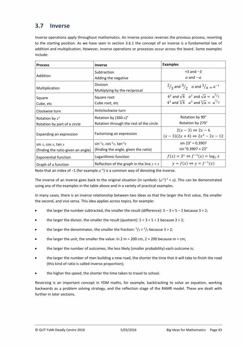
© QUT YuMi Deadly Centre 2016 5/03/2016 Big Ideas for Mathematics Page 43
3.7 Inverse
Inverse operations apply throughout mathematics. An inverse process reverses the previous process, reverting to the starting position. As we have seen in section 3.6.1 the concept of an inverse is a fundamental law of addition and multiplication. However, inverse operations or processes occur across the board. Some examples include:
Process Inverse Examples
Addition Subtraction Adding the negative
+3 and −3 𝑎𝑎 and −𝑎𝑎
Multiplication Division Multiplying by the reciprocal
23� and 3 2� 𝑎𝑎 and 1 𝑎𝑎 =� 𝑎𝑎−1
Square Cube, etc
Square root Cube root, etc
42 and √4 𝑎𝑎2 and √𝑎𝑎 = 𝑎𝑎1 2� 43 and √43 𝑎𝑎3 and √𝑎𝑎3 = 𝑎𝑎1 3�
Clockwise turn Anticlockwise turn
Rotation by x° Rotation by part of a circle
Rotation by (360-x)° Rotation through the rest of the circle
Rotation by 90° Rotation by 270°
Expanding an expression Factorising an expression 2(𝑥𝑥 − 3) ⇔ 2𝑥𝑥 − 6
(𝑥𝑥 − 3)(2𝑥𝑥 + 4) ⇔ 2𝑥𝑥2 − 2𝑥𝑥 − 12
sin x, cos x, tan x (finding the ratio given an angle)
sin-1x, cos-1x, tan-1x (finding the angle, given the ratio)
sin 23° = 0.3907 sin-10.3907 = 23°
Exponential function Logarithmic function 𝑓𝑓(𝑥𝑥) = 3𝑥𝑥 ⇔ 𝑓𝑓−1(𝑥𝑥) = log3 𝑥𝑥
Graph of a function Reflection of the graph in the line y = x 𝑦𝑦 = 𝑓𝑓(𝑥𝑥) ⇔ 𝑦𝑦 = 𝑓𝑓−1(𝑥𝑥)
Note that an index of −1 (for example a−1) is a common way of denoting the inverse.
The inverse of an inverse goes back to the original situation (in symbols: (a-1)-1 = a). This can be demonstrated using any of the examples in the table above and in a variety of practical examples.
In many cases, there is an inverse relationship between two ideas so that the larger the first value, the smaller the second, and vice versa. This idea applies across topics, for example:
• the larger the number subtracted, the smaller the result (difference): 5 – 3 < 5 – 2 because 3 > 2;
• the larger the divisor, the smaller the result (quotient): 5 ÷ 3 < 5 ÷ 2 because 3 > 2;
• the larger the denominator, the smaller the fraction: 5/3 < 5/2 because 3 > 2;
• the larger the unit, the smaller the value: in 2 m = 200 cm, 2 < 200 because m < cm;
• the larger the number of outcomes, the less likely (smaller probability) each outcome is;
• the larger the number of men building a new road, the shorter the time that it will take to finish the road (this kind of ratio is called inverse proportion);
• the higher the speed, the shorter the time taken to travel to school.
Reversing is an important concept in YDM maths, for example, backtracking to solve an equation, working backwards as a problem solving strategy, and the reflection stage of the RAMR model. These are dealt with further in later sections.
Page 44 Principle Big Ideas 5/03/2016 © QUT YuMi Deadly Centre 2016
3.8 Units of measure and instrumentation
The attribute and/or units used to measure an object leads to the form of measuring device. For example, mass is the force pushing downward, so a suitable measuring instrument is the length of a spring to which the mass is attached (the principle behind analogue scales) or the mass required to balance the object on a balance beam (the principle behind balancing scales). If the object and/or units of measurement are small, a more accurate measuring device is required, for example we would not choose to measure the length of a book using a trundle wheel. Similarly, if a high level of accuracy is needed, a more precise measuring device is required, for example we would not attempt to measure 100 g of nuts needed in a cake using the bathroom scales.
When comparing measurements or calculating with them, common units are required, for example, a 3 m by 20 cm rectangle does not have an area of 60 units, because we have to change to common units before calculating (this leads to the need for standard units). This is similar to the principal for comparing fractions, where a common denominator is required.
3.9 Formulae
A mathematical formula is a general fact or rule expressed using the symbols and conventions of algebra. It is an abstract description of the process used to calculate simplify a mathematical object. Quoting a standard formula in the solution to a problem is a common way of justifying the mathematical process used to solve that problem.
Where possible, students should develop mathematical formulae themselves, following a process such as:
1. identifying the process through experimentation or inquiry
2. verbally describing the process
3. describing the process in written sentences
4. describing the process in writing using “shorthand” (student’s own symbols)
5. describing the process using algebraic conventions (standard formulae)
6. proving the formula
(less experienced mathematicians may defer some of the later steps until their knowledge has deepened)
The emphasis should be on understanding the process, not memorising the formula. In many cases, formulae add to the cognitive load on students, for little benefit. For example, it is easier to find the perimeter of a polygon without the use of a formula. On the other hand, there are few alternatives to using the formula 𝑉𝑉 = 4
3𝜋𝜋𝑟𝑟3 to
find the volume of a sphere. Undue reliance on memorising formulae is an indication of instrumental knowledge (Skemp, 1976).
Formulae arise commonly in the study of areas and volumes, statistics and probability and advanced algebra and trigonometry, as the following list reveals.
• Perimeter formulae for shapes with some regularity can be reduced to multiples of side, for example, P = 4l (square); P = 2(l + w) (rectangle); and circumference circle = 2𝜋𝜋𝑟𝑟.
• Area formulae for regular shapes are based on the product of two perpendicular lengths, for example, A = ½bh, A = ½absinC or 𝐴𝐴 = �𝑠𝑠(𝑠𝑠 − 𝑎𝑎)(𝑠𝑠 − 𝑏𝑏)(𝑠𝑠 − 𝑐𝑐) where 𝑠𝑠 = 1
2(𝑎𝑎 + 𝑏𝑏 + 𝑐𝑐) (triangle); A = s2
(square); A = lw (rectangle); A = 𝜋𝜋𝑟𝑟2 (circle). Surface area formulae include 𝑆𝑆𝐴𝐴 = 2(𝑙𝑙𝑙𝑙 + 𝑑𝑑𝑙𝑙 + 𝑙𝑙𝑑𝑑) (rectangular prism); 𝑆𝑆𝐴𝐴 = 2𝜋𝜋𝑟𝑟(𝑟𝑟 + ℎ) (cylinder); 𝑆𝑆𝐴𝐴 = 𝜋𝜋𝑟𝑟(𝑟𝑟 + ℎ) (cone); 𝑆𝑆𝐴𝐴 = 4𝜋𝜋𝑟𝑟2 (sphere).
• Volume formulae are based on the product of three mutually perpendicular (orthogonal) lengths or an area and perpendicular height, for example V = Ah (prisms and cylinders) and V = 1/3Ah (pyramids and cones); V = 4
3� 𝜋𝜋𝑟𝑟3 (sphere).
© QUT YuMi Deadly Centre 2016 5/03/2016 Big Ideas for Mathematics Page 45
• Angle formulae including 180(n – 2) (interior angle sum of a polygon) and 360 (exterior supplementary angle sum of a polygon).
• Measures of central tendency, where the mean is the sum of scores divided by the number of scores, the median is the middle score when the data is arranged in order of size (that is, the score in the 𝑛𝑛+1
2 th
position) and the mode is the most common score.
• Measures of spread including highest score subtract lowest score (range), 1𝑛𝑛∑ (𝑥𝑥𝑖𝑖 − �̅�𝑥)𝑛𝑛𝑖𝑖=1 (average
deviation), �1𝑛𝑛∑ (𝑥𝑥𝑖𝑖 − �̅�𝑥)2𝑛𝑛𝑖𝑖=1 (standard deviation.
• Probability formulae, including 𝑃𝑃(𝑒𝑒) = 𝑛𝑛(𝑒𝑒)𝑛𝑛(𝑆𝑆)
, 𝑃𝑃(𝑛𝑛,𝑟𝑟) = 𝑛𝑛!(𝑛𝑛−𝑟𝑟)!
(permutations), 𝐶𝐶(𝑛𝑛,𝑟𝑟) = 𝑛𝑛!𝑟𝑟!(𝑛𝑛−𝑟𝑟)!
(combinations).
• Formulae used in advanced algebra including 𝑎𝑎(𝑏𝑏 + 𝑐𝑐) = 𝑎𝑎𝑏𝑏 + 𝑎𝑎𝑐𝑐 (distributive law); (𝑎𝑎 ± 𝑏𝑏)2 = 𝑎𝑎2 ± 2𝑎𝑎𝑏𝑏 + 𝑏𝑏2 (perfect square); (𝑎𝑎 + 𝑏𝑏)(𝑎𝑎 − 𝑏𝑏) = 𝑎𝑎2 − 𝑏𝑏2 (difference of two
squares), 𝑥𝑥 = −𝑏𝑏±�𝑏𝑏2−4𝑎𝑎𝑎𝑎2𝑎𝑎
(quadratic formula); (𝑥𝑥 + 𝑎𝑎)𝑛𝑛 = � �𝑛𝑛𝑘𝑘�𝑥𝑥𝑘𝑘𝑎𝑎𝑛𝑛−𝑘𝑘
𝑛𝑛
𝑘𝑘=0 (binomial expansion).
• Calculus makes extensive use of formulae for standard differentials and integrals (too many to list here).
• Trigonometry formulae, including sin 𝜃𝜃 = oppositehypotenuse
, cos𝜃𝜃 = adjacenthypotenuse
, tan𝜃𝜃 = adjacentopposite
(trigonometric
ratios), sin 𝐴𝐴𝑎𝑎
= sin 𝐵𝐵𝑏𝑏
= sin 𝐶𝐶𝑎𝑎
(sine rule); 𝑎𝑎2 = 𝑏𝑏2 + 𝑐𝑐2 = 2𝑏𝑏𝑐𝑐 cos𝐴𝐴 (cosine rule) and various
trigonometric identities too numerous to list here.

© QUT YuMi Deadly Centre 2016 5/03/2016 Big Ideas for Mathematics Page 47
4 Strategy and Modelling Big Ideas
Strategies are used when there are difficulties in finding an answer. A strategy big idea is a strategy that has uses across years and topics. Many strategies have a principle form, for example, compensation is both an operation principle related to identity and inverse and a strategy for computation, so sometimes an idea will appear in strategies as well as principles. As a strategy, the idea will be described as an action to solve a problem or complete an activity.
To be a big idea, strategies have to have a life and use beyond a topic and a year level. For example, there are particular strategies for basic facts that are not used elsewhere (e.g. doubles). These narrow-in-application strategies will not be included in this section.
4.1 Computation
4.1.1 Calculation
Separation
This addition strategy involves separating the situation/problem into parts, doing the parts separately, and then combine them at the end. The strategy is used in traditional algorithms with whole and decimal numbers and extends to measures and algebra, for example,
35 + 21 = (30 + 20) + (5 + 1) = 56 separating by place value
2𝑥𝑥 + 3𝑦𝑦 + 4𝑥𝑥 − 𝑦𝑦 = 2𝑥𝑥 + 4𝑥𝑥 + 3𝑦𝑦 − 𝑦𝑦 = 6𝑥𝑥 + 2𝑦𝑦 separating by variable
It also applies to subtraction, with regrouping if necessary, for example,
75 – 48 = (70 – 40) + (5 – 8) = (70 – 50 + 10) + (5 – 8) = (70 – 50) + (10 + 5 – 8) = 20 + 7 = 27 separating by place value regrouping
The strategy is simpler if subtracting is treated as adding the negative
75 – 48 = (70 – 40) + (5 – 8) = 30 – 3 = 27 separating by place value
Sequencing
This addition strategy involves selecting one number as a starting position, separating the other number into its component parts and combining each part with the starting number step by step. For example,
347 + 236 = 347 + 200 + 36 = 547 + 30 + 6 = 577 + 6 = 583 hundreds tens ones
531 – 387 = 531 – 300 – 87 = 231 – 80 – 7 = 151 – 7 = 144 hundreds tens ones
This method is particularly effective for mental computation because the digits in the second number are processed one at a time.
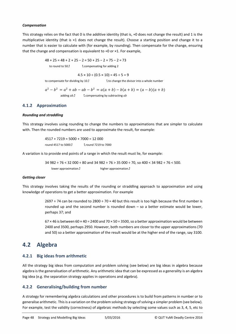
Page 48 Strategy and Modelling Big Ideas 5/03/2016 © QUT YuMi Deadly Centre 2016
Compensation
This strategy relies on the fact that 0 is the additive identity (that is, +0 does not change the result) and 1 is the multiplicative identity (that is ×1 does not change the result). Choose a starting position and change it to a number that is easier to calculate with (for example, by rounding). Then compensate for the change, ensuring that the change and compensation is equivalent to +0 or ×1. For example,
48 + 25 = 48 + 2 + 25 – 2 = 50 + 25 − 2 = 75 – 2 = 73 to round to 50 compensating for adding 2
4.5 × 10 ÷ (0.5 × 10) = 45 ÷ 5 = 9 to compensate for dividing by 10 to change the divisor into a whole number
𝑎𝑎2 − 𝑏𝑏2 = 𝑎𝑎2 + 𝑎𝑎𝑏𝑏 − 𝑎𝑎𝑏𝑏 − 𝑏𝑏2 = 𝑎𝑎(𝑎𝑎 + 𝑏𝑏) − 𝑏𝑏(𝑎𝑎 + 𝑏𝑏) = (𝑎𝑎 − 𝑏𝑏)(𝑎𝑎 + 𝑏𝑏)
adding ab compensating by subtracting ab
4.1.2 Approximation
Rounding and straddling
This strategy involves using rounding to change the numbers to approximations that are simpler to calculate with. Then the rounded numbers are used to approximate the result, for example:
4517 + 7219 ≈ 5000 + 7000 = 12 000 round 4517 to 5000 round 7219 to 7000
A variation is to provide end points of a range in which the result must lie, for example:
34 982 ÷ 76 < 32 000 ÷ 80 and 34 982 ÷ 76 > 35 000 ÷ 70, so 400 < 34 982 ÷ 76 < 500. lower approximation higher approximation
Getting closer
This strategy involves taking the results of the rounding or straddling approach to approximation and using knowledge of operations to get a better approximation. For example
2697 ÷ 74 can be rounded to 2800 ÷ 70 = 40 but this result is too high because the first number is rounded up and the second number is rounded down – so a better estimate would be lower, perhaps 37; and
67 × 46 is between 60 × 40 = 2400 and 70 × 50 = 3500, so a better approximation would be between 2400 and 3500, perhaps 2950. However, both numbers are closer to the upper approximations (70 and 50) so a better approximation of the result would be at the higher end of the range, say 3100.
4.2 Algebra
4.2.1 Big ideas from arithmetic
All the strategy big ideas from computation and problem solving (see below) are big ideas in algebra because algebra is the generalisation of arithmetic. Any arithmetic idea that can be expressed as a generality is an algebra big idea (e.g. the separation strategy applies in operations and algebra).
4.2.2 Generalising/building from number
A strategy for remembering algebra calculations and other procedures is to build from patterns in number or to generalise arithmetic. This is a variation on the problem solving strategy of solving a simpler problem (see below). For example, test the validity (correctness) of algebraic methods by selecting some values such as 3, 4, 5, etc to
© QUT YuMi Deadly Centre 2016 5/03/2016 Big Ideas for Mathematics Page 49
use in place of the variables (substitute). If the result is a true statement using that set of numbers, try again with a different set of numbers. It is highly likely that if the algebraic method works for two different sets of numbers, then method is valid. However, avoid using 0 and 1 (the additive and multiplicative identities) or 2 (because of the relation 2 × 2 = 2 + 2) as test values because they can produce some results that are hard to interpret.
4.3 Measurement
Measurement is the application of computation and problem solving to quantities, so most measurement strategies are dealt with elsewhere. However, the following two strategies have not yet been discussed.
4.3.1 Using an intermediary
In comparing or measuring objects a concrete intermediary (e.g. string for length, tessellating shapes for area) can assist on the way to the use of units.
4.3.2 Not confusing steps with end points
The starting point when counting is 1, but when measuring it is 0. For example, if a person worked at McDonalds throughout 2002 to 2006, that is from 1 Jan 2002 to 31 Dec 2006, then they worked at McDonalds for 5 years (as shown in the table below) even though 2006 − 2002 = 4. This is because the year (2002) names the step and the time is the difference between the start of the first step and the end of the last step.
Calendar year (1 Jan) 2002 2003 2004 2005 2006 2007 – 1 day
Cumulative number of years worked 0 1 2 3 4 5
Similarly, a fence with 6 panels needs 7 fence posts.
4.4 Visualising
Visualisation is an important strategy in many situations. It is the basis of the third part of the body→hand→mind process. In cases where it is impossible or impractical to act out a process or to use concrete materials, students must visualise. Many NAPLAN questions require visualisation.
4.4.1 Shapes
Transformations
In your mind, reflect (flip), rotate (turn) or translate (slide) the object. This assists in determining if two shapes are the same or different, in undertaking tessellation and dissection puzzles, and in determining direction of projective activities.
Identify the difficult piece, activity or placement
Look at the activity and determine the most complex piece and place it first; identify what would be confusing in the activity and try to do that first; and identify the difficult placement and try to find many ways to complete it (even if you have to use two pieces).
4.4.2 Visual images
Visual representations, or visuals, such as diagrams, illustrations, photographs, scale drawings, maps, charts, figures, icons, graphs, plots, networks, sketches, animations, and plans are an important form of mathematics communication, in school and extending into post-school education, training, and employment. Perusal of most school mathematics textbooks reveals that visuals appear on almost every page. Assessment items such as NAPLAN tests also make extensive use of visuals. The expectation that students of mathematics should be able
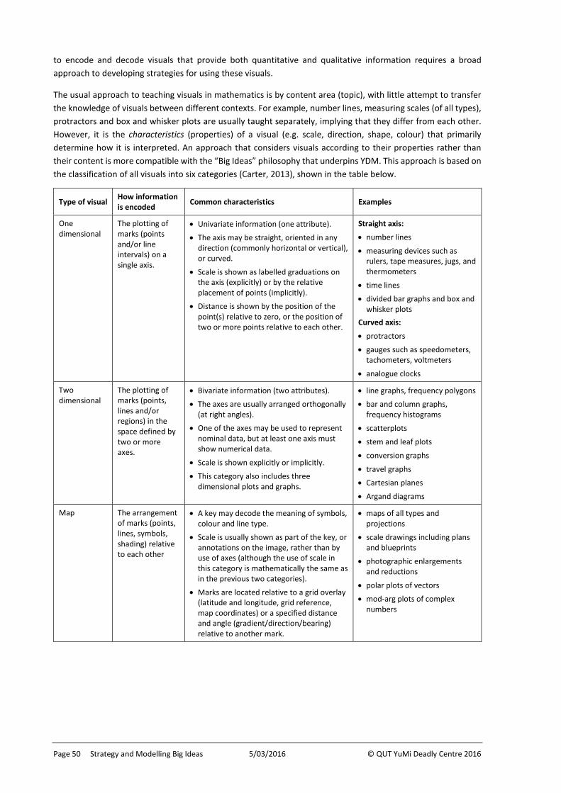
Page 50 Strategy and Modelling Big Ideas 5/03/2016 © QUT YuMi Deadly Centre 2016
to encode and decode visuals that provide both quantitative and qualitative information requires a broad approach to developing strategies for using these visuals.
The usual approach to teaching visuals in mathematics is by content area (topic), with little attempt to transfer the knowledge of visuals between different contexts. For example, number lines, measuring scales (of all types), protractors and box and whisker plots are usually taught separately, implying that they differ from each other. However, it is the characteristics (properties) of a visual (e.g. scale, direction, shape, colour) that primarily determine how it is interpreted. An approach that considers visuals according to their properties rather than their content is more compatible with the “Big Ideas” philosophy that underpins YDM. This approach is based on the classification of all visuals into six categories (Carter, 2013), shown in the table below.
Type of visual How information is encoded Common characteristics Examples
One dimensional
The plotting of marks (points and/or line intervals) on a single axis.
• Univariate information (one attribute).
• The axis may be straight, oriented in any direction (commonly horizontal or vertical), or curved.
• Scale is shown as labelled graduations on the axis (explicitly) or by the relative placement of points (implicitly).
• Distance is shown by the position of the point(s) relative to zero, or the position of two or more points relative to each other.
Straight axis:
• number lines
• measuring devices such as rulers, tape measures, jugs, and thermometers
• time lines
• divided bar graphs and box and whisker plots
Curved axis:
• protractors
• gauges such as speedometers, tachometers, voltmeters
• analogue clocks
Two dimensional
The plotting of marks (points, lines and/or regions) in the space defined by two or more axes.
• Bivariate information (two attributes).
• The axes are usually arranged orthogonally (at right angles).
• One of the axes may be used to represent nominal data, but at least one axis must show numerical data.
• Scale is shown explicitly or implicitly.
• This category also includes three dimensional plots and graphs.
• line graphs, frequency polygons
• bar and column graphs, frequency histograms
• scatterplots
• stem and leaf plots
• conversion graphs
• travel graphs
• Cartesian planes
• Argand diagrams
Map The arrangement of marks (points, lines, symbols, shading) relative to each other
• A key may decode the meaning of symbols, colour and line type.
• Scale is usually shown as part of the key, or annotations on the image, rather than by use of axes (although the use of scale in this category is mathematically the same as in the previous two categories).
• Marks are located relative to a grid overlay (latitude and longitude, grid reference, map coordinates) or a specified distance and angle (gradient/direction/bearing) relative to another mark.
• maps of all types and projections
• scale drawings including plans and blueprints
• photographic enlargements and reductions
• polar plots of vectors
• mod-arg plots of complex numbers
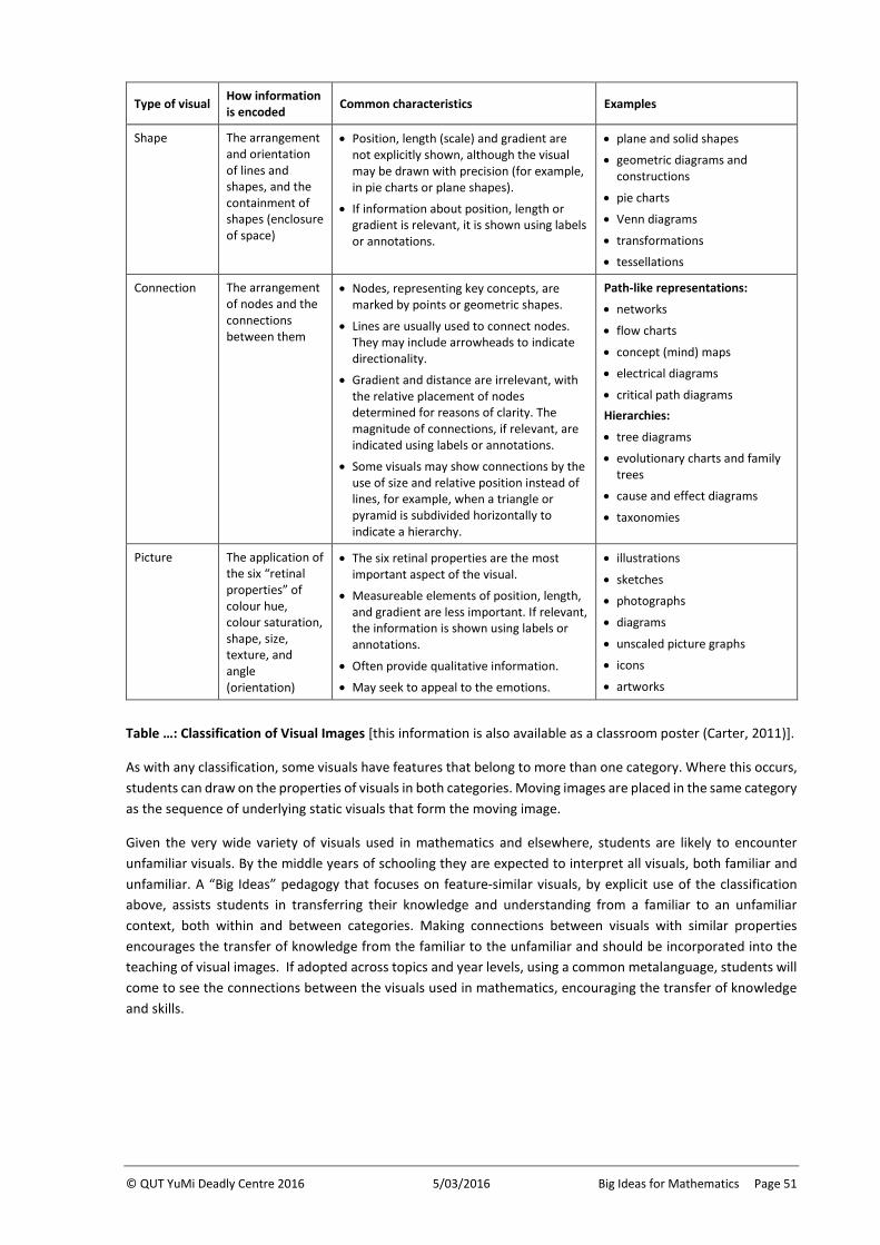
© QUT YuMi Deadly Centre 2016 5/03/2016 Big Ideas for Mathematics Page 51
Type of visual How information is encoded Common characteristics Examples
Shape The arrangement and orientation of lines and shapes, and the containment of shapes (enclosure of space)
• Position, length (scale) and gradient are not explicitly shown, although the visual may be drawn with precision (for example, in pie charts or plane shapes).
• If information about position, length or gradient is relevant, it is shown using labels or annotations.
• plane and solid shapes
• geometric diagrams and constructions
• pie charts
• Venn diagrams
• transformations
• tessellations
Connection The arrangement of nodes and the connections between them
• Nodes, representing key concepts, are marked by points or geometric shapes.
• Lines are usually used to connect nodes. They may include arrowheads to indicate directionality.
• Gradient and distance are irrelevant, with the relative placement of nodes determined for reasons of clarity. The magnitude of connections, if relevant, are indicated using labels or annotations.
• Some visuals may show connections by the use of size and relative position instead of lines, for example, when a triangle or pyramid is subdivided horizontally to indicate a hierarchy.
Path-like representations:
• networks
• flow charts
• concept (mind) maps
• electrical diagrams
• critical path diagrams Hierarchies:
• tree diagrams
• evolutionary charts and family trees
• cause and effect diagrams
• taxonomies
Picture The application of the six “retinal properties” of colour hue, colour saturation, shape, size, texture, and angle (orientation)
• The six retinal properties are the most important aspect of the visual.
• Measureable elements of position, length, and gradient are less important. If relevant, the information is shown using labels or annotations.
• Often provide qualitative information.
• May seek to appeal to the emotions.
• illustrations
• sketches
• photographs
• diagrams
• unscaled picture graphs
• icons
• artworks
Table …: Classification of Visual Images [this information is also available as a classroom poster (Carter, 2011)].
As with any classification, some visuals have features that belong to more than one category. Where this occurs, students can draw on the properties of visuals in both categories. Moving images are placed in the same category as the sequence of underlying static visuals that form the moving image.
Given the very wide variety of visuals used in mathematics and elsewhere, students are likely to encounter unfamiliar visuals. By the middle years of schooling they are expected to interpret all visuals, both familiar and unfamiliar. A “Big Ideas” pedagogy that focuses on feature-similar visuals, by explicit use of the classification above, assists students in transferring their knowledge and understanding from a familiar to an unfamiliar context, both within and between categories. Making connections between visuals with similar properties encourages the transfer of knowledge from the familiar to the unfamiliar and should be incorporated into the teaching of visual images. If adopted across topics and year levels, using a common metalanguage, students will come to see the connections between the visuals used in mathematics, encouraging the transfer of knowledge and skills.
Page 52 Strategy and Modelling Big Ideas 5/03/2016 © QUT YuMi Deadly Centre 2016
4.5 Statistical inference
4.5.1 Sampling
The focus of statistical inference is to make decisions about the particular, using thinking and processes that are more generic. Uniquely to statistics, a part (sample) is used to make findings about the whole (population). Certainty can be improved by ensuring appropriate relationships between the sample and population, for example by selecting the sample in an unbiased manner so that it represents the population. There are various strategies for selecting an appropriate sample, including:
• random selection, using a process that is truly random such as drawing lots, use of the random number generator in a calculator or computer, or (historically) the use of a table of random numbers
• systematic selection, where a starting position is selected randomly and then items are selected at regular
intervals thought the population, using a formula such as population size
desired sample size to determine the size of the
intervals
• stratified sampling, where the population is classified into strata according to pre-determined characteristics (for example, gender, age, occupation, city/regional/remote residents) and a random sample is taken from each strata so that they are represented in the overall sample in the same proportions as in the population
• cluster sampling, where the population is divided into clusters (often based on location), and then clusters are selected randomly, with the sample drawn randomly from the selected clusters.
4.5.2 Enumerating
When calculating theoretical probabilities, the size of both the sample space (the population) and the event (the group satisfying desired condition) are needed. For example, to calculate the probability of a selecting a red marble from a bag, both the number of red marbles (the event) and the total number of marbles in the bag (the population) must be known. In simple (one stage) probability events, this information is usually easy to obtain. However, in complex, multi-stage events it can be harder to find the number in the event and/or the number in the sample space.
The number in the event and the sample space is affected by way in which the sample is selected: with or without replacement. For example, when selecting several marbles from a bag, if the chosen marble is returned to the bag before the next selection is made, the number in the event and the sample space do not change. However, if the chosen marble is set aside (not replaced) before the next selection is made, then the total number of marbles in the bag and the number of marbles of the same colour as the chosen marble are both reduced by one.
There are various strategies for finding the number in the sample space and the event, including:
• grids: useful for identifying the outcomes in two-stage events with replacement, impractical if the sample space is large
• tree diagrams: useful for investigating the outcomes in multi-stage events with and without replacement, but impractical if the sample space is large
• Venn diagrams: useful for two and three stage events with replacement
• multiplication principle: useful for useful for investigating outcomes from large populations with multi-stage events with and without replacement, for example, the number of different four-digit PIN number combinations is 10 × 10 × 10 × 10 (a “with replacement” situation); whereas the number of ways of arranging four different coloured blocks is 4 × 3 × 2 × 1 (a “without replacement” situation)
© QUT YuMi Deadly Centre 2016 5/03/2016 Big Ideas for Mathematics Page 53
• combinations and permutations: useful for investigating outcomes without replacement from large populations, including when the order in which the outcomes are selected are important (permutations) or do not matter (combinations).
4.6 Problem solving
4.6.1 Metacognition
This is the ability to oversee, monitor and evaluate thinking, to plan and check, and in the final analysis, to be aware of own thinking. Metacognitive ability is often operationalised by the adoption of a plan of attack.
4.6.2 Plans of attack
The initial starting point for problems is a plan of attack. One of the best is Polya’s (1957) four stage model:
• SEE – use strategies to understand what problem wants;
• PLAN – prepare a plan of strategies to solve the problem;
• DO – act out the plan and attempt to solve the problem; and
• CHECK – check answer and reflect on what was effective in the process.
4.6.3 Thinking skills
These are abilities to engage in a variety of types of thinking:
• logical (and consistent) – see the discussion of the global big idea on logical structure, starting on page 10;
• visual (and spatial) – see the discussion of visualising, starting on page 47;
• evaluative/validating (to check, evaluate and make decisions);
• patterning (to find, continue and solve patterns) – see the discussion of the global big idea on patterns, starting on page 14; and
• creative/flexible (to have access to many options, and to be able to find a new direction).
These thinking skills are related to the problem solving strategies (see below).
4.6.4 Strategies
Strategies are general rules of thumb that point the direction to an answer – they enable you to work out what to do when you don’t know what to do. They are clustered with thinking skills as follows.
• Logical/language cluster – includes: “reread the question”, “identify given, needed and wanted”, “restate the problem” and “write a number sentence”.
• Visual/spatial cluster – includes: “act it out”, “make a model”, “make a drawing, diagram or graph” and “select appropriate notation to picture the problem”.
• Evaluating/validating/checking cluster – includes: “generalising the solution”, “checking the solution”, “finding another way to solve it”, “finding another solution” and “studying the solution process”.
• Patterning/organising cluster – includes: “look for a pattern”, “construct a table” and “account for all possibilities (systematically)”.
• Creative/flexible/restructuring cluster – includes: “guess and check”, “work backwards”, “identify a sub-goal (break problem into parts)”, “solve a simpler problem”, “change your point of view” and “check for hidden assumptions”.
Page 54 Strategy and Modelling Big Ideas 5/03/2016 © QUT YuMi Deadly Centre 2016
The YDM Supplementary Book 2 examines Problem Solving in more detail.
4.7 Mathematical modelling
Models are conceptual processes used to construct, describe, explain and/or predict the behaviour of complex systems (English, 2008). Mathematical models differ from other categories of models mainly because they focus on structural characteristics (rather than, for example, physical, biological, or artistic characteristics) of the systems they describe (Lesh & Harel, 2003). They are underpinned by quantitative processes (for example, counting, measuring, calculating, graphing, inferring, extrapolating), although they may also include qualitative methods (such as describing and explaining).
Mathematical models can be represented in a variety of ways, including language (written and spoken), symbols, visual images/graphics (both computer- and paper-based), or experience-based metaphors. They generally have two parts: a conceptual system for describing or explaining the relevant mathematical objects, relations, actions, patterns, and regularities; and accompanying procedures for generating useful constructions, manipulations, or predictions for achieving clearly recognized goals (Lesh & Harel, 2003).
The process of developing, applying, evaluating, and modifying mathematical models is known as mathematical modelling.
4.7.1 More extensive than problem solving
Although often associated with problem solving, mathematical modelling involves more than responding to well formulated word questions, where the student is expected to find the wanted information from the given information (Lesh & Harel, 2003). Modelling is associated with open-ended, inquiry based investigations. Specifically modelling differs from problem solving in several respects (Box, 1976; Doyle, 2006; English, 2008; Lesh & Harel, 2003).
• Mathematical modelling goes beyond the traditional form of problem solving where the key mathematical ideas are presented “up front” and students select an appropriate solution strategy to produce a single, usually brief, response. In contrast, modelling problems have the important mathematical ideas embedded within the problem context for students to discover as they work the problem.
• The problems are often multidisciplinary: they can relate to learning areas beyond mathematics.
• The strategies and processes that are most useful for modelling tend to differ from those that used for traditional problem solving: modelling typically uses mathematical processes such as constructing, describing, explaining, predicting, and representing, together with organizing, coordinating, quantifying, and transforming data.
• The development of a model generally involves cycles in which students’ thinking must be tested, retested and revised.
• The model can usually deal with more than one instance: it is reusable (in other situations), shareable (with other people), and/or modifiable (for other purposes).
• Modelling problems are multifaceted: students’ final products encompass a variety of representational formats including written text, graphs, tables, diagrams, spreadsheets, and oral reports
• Students may be required to make initial assumptions about the situation. Whilst these assumptions may be false, they can reduce the complexity of the model, whilst producing results that are useful approximations of the real world. The effect of any assumptions should be examined as part of the process of evaluating the model.
© QUT YuMi Deadly Centre 2016 5/03/2016 Big Ideas for Mathematics Page 55
• In most modelling situations where mathematical processes must be developed, it is clear why and for whom, the process is needed, providing a way of evaluating the model.
• There are often a range of acceptable approaches, representations and solutions.
• Numerical values, if produced by the model, tend to be probabilistic (that is, an estimate of the most likely value) rather than absolutist.
4.7.2 Process
The process of mathematical modelling commences with a problem (usually life-related) that requires a model to describe, explain, or predict the behaviour of a given system (this is called a model-eliciting problem). There are six principles that can be applied to ensure that a problem will lead to the development of a mathematical model, summarised below (Lesh, Cramer, Doerr, Post, & Zawojewski, 2003).
• Is the problem realistic – could it really happen? Will the students’ range of responses to the problem all be taken seriously or will they be required to conform to a ‘correct’ solution?
• Does the task specification clearly ensure that there is a need to construct a mathematical model?
• Are there clear criteria that students are able to self-evaluate the usefulness of the model?
• What mathematical ideas should the students be thinking about, and does the task prompt the students to make that thinking explicit?
• Is the problem as simple as possible without compromising the need to create a model?
• Will the model that is generated lend itself to re-application or generalising to new problem contexts?
The student commences the modelling process by identifying the essential elements or features that are of interest to the situation to be modelled (English, 2008; Stillman, Brown, & Geiger, 2015). Research may be necessary. In the process of using mathematics to model the real world we make tentative assumptions, which we know to be false, but simplify the situation to be modelled (for example, “let’s ignore … for the moment, what would happen then?”). In some cases, the simpler situation can yield useful approximations of results found in the real world (Box, 1976). These simpler problems can be explored to find relations and patterns that can be refined, extended, generalised and abstracted back to the original problem. It may require the translation of information into alternative representations (for example, from a description to a table). Patterns are most easily observed in graphs. This process of formulating an ideal problem from the real situation is known as idealisation.
The idealised situation is mathematised through translation into the mathematical domain. The mathematical domain includes the mathematical model made of the situation, mathematical questions posed and mathematical artefacts (e.g., graphs and tables) used to solve the mathematical model.
Since a mathematical model usually involves a simplification and/or generalisation of the real world, it can never produce accurate results. The process of mathematical modelling becomes a trade-off between simplicity and accuracy. The challenge is to find a model where the real world situation is simplified through the use of assumptions to remove complexity, but which nevertheless yields useful results, that is, results that are close approximations of reality. This raises two important questions. First, how do we know that the modelled results are close approximations of reality? Second, what is the effect of those assumptions? To answer the first question, the outputs of the mathematical model (i.e., answers) have to be interpreted in the context of the real situation that stimulated the modelling (for example, by comparing the model’s outputs with known values). In the case of the second question, changing the assumptions can show how sensitive the model is to those assumptions. A useful model is one where changes to the assumptions make little difference to the outputs or the conclusions drawn from those outputs.

Page 56 Strategy and Modelling Big Ideas 5/03/2016 © QUT YuMi Deadly Centre 2016
Successful mathematical modelling may lead to model exploration activities (the construction of alternate models and the use of more abstract representations), or model adaptation activities (the use of generalised, abstract model in new situations, leading to more formal examination of the applicable mathematical structures) (Lesh, et al., 2003).
© QUT YuMi Deadly Centre 2016 5/03/2016 Big Ideas for Mathematics Page 57
5 Pedagogy Big Ideas
Mathematics content that is connected can be taught using similar materials and techniques. For example, whole-number place value, decimal-number place value, metric conversions, and mixed numbers can all use the same teaching materials and techniques. The use of similar materials and techniques to teach concepts can help to reinforce the connections between those concepts. This is the basis of the “Big Ideas” approach to pedagogy.
5.1 Structure
In YDM, pedagogy is in two parts: (a) the sequencing and connecting of big ideas across the years of schooling; and (b) the processes involved in teaching a step in this sequence. The big ideas in this sub-section relate to the structure of mathematics.
5.1.1 Groups, wholes and parts
In mathematics, the idea of a “whole” is referred to as a unit. Anything can be a unit: a single object, a collection of objects, a section of a line, a collection of lines. Units can form groups and units can be partitioned into parts. For example, if there are six counters:
• each counter can be a unit forming a group of six units; or
• the set of six counters can be a unit, forming one unit with six parts.
The relationship between groups, parts and wholes can be reversed to ensure that connections are made in both directions. For example:
• 3⁄4 of 12 is 9 (whole part); and
• if 3⁄4 of a whole is 12 means that the whole is 16 (part whole).
The idea of a unit underpins work in place value, fractions (decimal and common), percentages, ratios, measurement, algebra, and probability. It also contributed to the understanding of pedagogical models such as part-part-whole and factor-factor-product described in sub-section 5.7.
5.1.2 Triadic relations
When three things are related by an action, the process can be described generically is a * b = c. There are three possible unknowns a, b or c, leading to three problem types: find a, find b or find c. For example, given 2 + 3 = 5, problems can be written for ? + 3 = 5, 2 + ? = 5, or 2 + 3 = ?; similarly given that 25% of $88 is $22, the following questions can be posed: what percentage of 88 is 22?, if 25% is 22 what is 100%?, or what is 25% of 88?.
Exploring triadic relations is an aspect of reflection in the RAMR model (see sub-section 5.4). All problem types should be taught.
5.2 Sequencing
These big ideas are to ensure ideas are sequenced to maximise learning.
5.2.1 Pre-empting and peeling back
Pre-empting is the process of looking forward when planning lessons so that what is taught earlier supports, rather than complicates, teaching in later years. An example is that partwhole approach to fractions teaches
Page 58 Pedagogy Big Ideas 5/03/2016 © QUT YuMi Deadly Centre 2016
fractions better and also prepares for a similar partwhole approach to percentages. In another example, the possibility of negative numbers should always be accommodated, even with very young students. Rather than teaching that 3 – 5 is not possible, tell students that it produces a negative result, which they will learn about later. Otherwise, problems arise when explaining subtraction with regrouping (such as 63 – 35) and the existence of negative numbers.
Peeling back involves looking backward and building on what previous teachers have done. This allows for a connected approach in developing big ideas. Using the example in the previous paragraph, taking a partwhole approach to teaching percentages builds on the partwhole approach used with fractions in the past, as well as emphasising the connections between fractions and percentages. Peeling back is also a sound approach to remediation – prior learning is ‘peeled back’ until the missing or erroneous pre-requisite knowledge is located. Once the gap or misconception is remedied, later work can be rebuilt on solid foundations.
Pre-empting and peeling back both require a knowledge of what went before and what comes later. It is one of the reasons that this book discusses the big ideas of mathematics across the full range of schooling.
5.2.2 Seamlessness
Seamless sequences should lead from old to new work. For example, multiplying by ten (× 10) should not be taught as adding a zero to the right hand side of the number – it leads to decimal errors. If students learn that × 10 moves place value positions to the left, the same idea can be applied to decimals. It is true that, for whole numbers, × 10 means a zero place holder has to be added and, for decimals, × 10 means that the decimal point moves to right, but these are the consequences of multiplying by ten and must not be confused with the process of multiplying by 10.
Look for ways to ensure connections are made. For example, show that base and (perpendicular) height are the same ideas in triangles and quadrilaterals, although they might also be called side, length, depth, or width. Regularly use vertical algorithms for algebra and horizontal presentations for arithmetic so students can see the relation of number to algebra.
5.2.3 Compromise and reteaching
The psycho-logic of the child is not the same as the logical structure of mathematics. This requires compromises in the way that mathematical teaching is sequenced. Everything cannot be taught in a finished state. For example, 1–1 correspondence is taught in Year P, and then extended to 1–many correspondence in Year 2; abstraction from stories to number is developed in the early years, but further abstraction to formal algebra does not occur until Year 7. Education is a process of continually teaching, unteaching and reteaching. Be aware when these reteachings are required and allow extra time.
5.3 Pedagogical approaches
5.3.1 Imitative
In imitative pedagogies, students imitate the teacher’s knowledge through approaches such as “I do, we do, you do”, for example the Gradual Withdrawal of Support model by Fisher and Frey (2008). Such approaches are also referred to as structured teaching or explicit teaching.
Whilst not a big part of the YDM approach, imitative pedagogies have their place. They can be useful in teaching processes, for example students are unlikely to learn how to write mathematically unless shown by a teacher. They can also be a more efficient use of time in the short-term; however, if they do not result in relational learning (Skemp, 1976) students may have difficulty in understanding or recalling concepts, requiring later reteaching and may ultimately be a less efficient use of time.
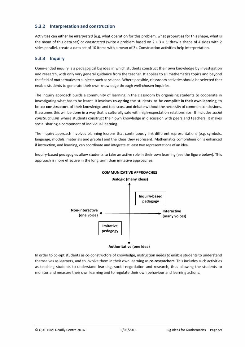
© QUT YuMi Deadly Centre 2016 5/03/2016 Big Ideas for Mathematics Page 59
5.3.2 Interpretation and construction
Activities can either be interpreted (e.g. what operation for this problem, what properties for this shape, what is the mean of this data set) or constructed (write a problem based on 2 + 3 = 5; draw a shape of 4 sides with 2 sides parallel, create a data set of 10 items with a mean of 3). Construction activities help interpretation.
5.3.3 Inquiry
Open-ended inquiry is a pedagogical big idea in which students construct their own knowledge by investigation and research, with only very general guidance from the teacher. It applies to all mathematics topics and beyond the field of mathematics to subjects such as science. Where possible, classroom activities should be selected that enable students to generate their own knowledge through well-chosen inquiries.
The inquiry approach builds a community of learning in the classroom by organising students to cooperate in investigating what has to be learnt. It involves co-opting the students to be complicit in their own learning, to be co-constructors of their knowledge and to discuss and debate without the necessity of common conclusions. It assumes this will be done in a way that is culturally safe with high-expectation relationships. It includes social constructivism where students construct their own knowledge in discussion with peers and teachers. It makes social sharing a component of individual learning.
The inquiry approach involves planning lessons that continuously link different representations (e.g. symbols, language, models, materials and graphs) and the ideas they represent. Mathematics comprehension is enhanced if instruction, and learning, can coordinate and integrate at least two representations of an idea.
Inquiry-based pedagogies allow students to take an active role in their own learning (see the figure below). This approach is more effective in the long term than imitative approaches.
In order to co-opt students as co-constructors of knowledge, instruction needs to enable students to understand themselves as learners, and to involve them in their own learning as co-researchers. This includes such activities as teaching students to understand learning, social negotiation and research, thus allowing the students to monitor and measure their own learning and to regulate their own behaviour and learning actions.
COMMUNICATIVE APPROACHES
Inquiry-based pedagogy
Dialogic (many ideas)
Authoritative (one idea)
Interactive (many voices)
Non-interactive (one voice)
Imitative pedagogy
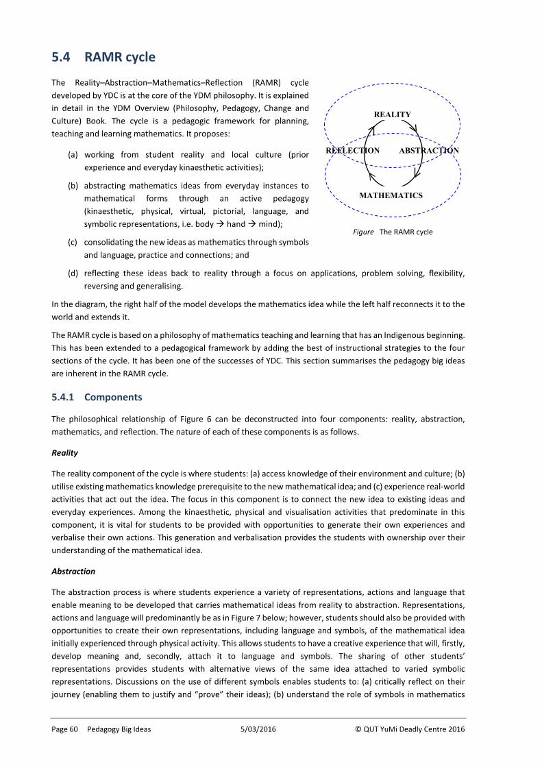
Page 60 Pedagogy Big Ideas 5/03/2016 © QUT YuMi Deadly Centre 2016
5.4 RAMR cycle
The Reality–Abstraction–Mathematics–Reflection (RAMR) cycle developed by YDC is at the core of the YDM philosophy. It is explained in detail in the YDM Overview (Philosophy, Pedagogy, Change and Culture) Book. The cycle is a pedagogic framework for planning, teaching and learning mathematics. It proposes:
(a) working from student reality and local culture (prior experience and everyday kinaesthetic activities);
(b) abstracting mathematics ideas from everyday instances to mathematical forms through an active pedagogy (kinaesthetic, physical, virtual, pictorial, language, and symbolic representations, i.e. body hand mind);
(c) consolidating the new ideas as mathematics through symbols and language, practice and connections; and
(d) reflecting these ideas back to reality through a focus on applications, problem solving, flexibility, reversing and generalising.
In the diagram, the right half of the model develops the mathematics idea while the left half reconnects it to the world and extends it.
The RAMR cycle is based on a philosophy of mathematics teaching and learning that has an Indigenous beginning. This has been extended to a pedagogical framework by adding the best of instructional strategies to the four sections of the cycle. It has been one of the successes of YDC. This section summarises the pedagogy big ideas are inherent in the RAMR cycle.
5.4.1 Components
The philosophical relationship of Figure 6 can be deconstructed into four components: reality, abstraction, mathematics, and reflection. The nature of each of these components is as follows.
Reality
The reality component of the cycle is where students: (a) access knowledge of their environment and culture; (b) utilise existing mathematics knowledge prerequisite to the new mathematical idea; and (c) experience real-world activities that act out the idea. The focus in this component is to connect the new idea to existing ideas and everyday experiences. Among the kinaesthetic, physical and visualisation activities that predominate in this component, it is vital for students to be provided with opportunities to generate their own experiences and verbalise their own actions. This generation and verbalisation provides the students with ownership over their understanding of the mathematical idea.
Abstraction
The abstraction process is where students experience a variety of representations, actions and language that enable meaning to be developed that carries mathematical ideas from reality to abstraction. Representations, actions and language will predominantly be as in Figure 7 below; however, students should also be provided with opportunities to create their own representations, including language and symbols, of the mathematical idea initially experienced through physical activity. This allows students to have a creative experience that will, firstly, develop meaning and, secondly, attach it to language and symbols. The sharing of other students’ representations provides students with alternative views of the same idea attached to varied symbolic representations. Discussions on the use of different symbols enables students to: (a) critically reflect on their journey (enabling them to justify and “prove” their ideas); (b) understand the role of symbols in mathematics
REALITY
MATHEMATICS
ABSTRACTION REFLECTION
Figure The RAMR cycle
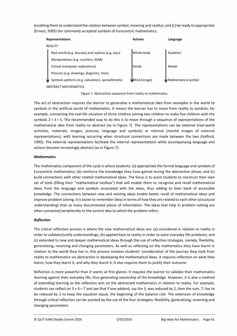
© QUT YuMi Deadly Centre 2016 5/03/2016 Big Ideas for Mathematics Page 61
(enabling them to understand the relation between symbol, meaning and reality); and (c) be ready to appropriate (Ernest, 2005) the commonly accepted symbols of Eurocentric mathematics.
Representations Actions Language
REALITY
Real world (e.g. biscuits) and replicas (e.g. toys) Whole body Students’
Manipulatives (e.g. counters, MAB)
Virtual (computer replications) Hands Model
Pictures (e.g. drawings, diagrams, lines)
Symbols patterns (e.g. calculators, spreadsheets) Mind (image) Mathematics/symbol
ABSTRACT MATHEMATICS
Figure 1 Abstraction sequence from reality to mathematics
The act of abstraction requires the learner to generalise a mathematical idea from examples in the world to symbols in the artificial world of mathematics. It means the learner has to move from reality to symbols; for example, connecting the real-life situation of three children joining two children to make five children with the symbols 2 + 3 = 5. The recommended way to do this is to move through a sequence of representations of the mathematical idea from reality to abstract (as in Figure 7). The representations can be external (real-world activities, materials, images, pictures, language and symbols) or internal (mental images of external representations), with learning occurring when structural connections are made between the two (Halford, 1993). The external representations facilitate the internal representations while accompanying language and actions become increasingly abstract (as in Figure 7).
Mathematics
The mathematics component of the cycle is where students: (a) appropriate the formal language and symbols of Eurocentric mathematics; (b) reinforce the knowledge they have gained during the abstraction phase; and (c) build connections with other related mathematical ideas. The focus is to assist students to construct their own set of tools (filling their “mathematical toolbox”) that will enable them to recognise and recall mathematical ideas from the language and symbols associated with the ideas, thus adding to their bank of accessible knowledge. The connections between new and existing ideas enable better recall of mathematical ideas and improve problem solving. It is easier to remember ideas in terms of how they are related to each other (structural understanding) than as many disconnected pieces of information. The ideas that help in problem solving are often connected peripherally to the central idea to which the problem refers.
Reflection
The critical reflection process is where the new mathematical ideas are: (a) considered in relation to reality in order to validate/justify understandings; (b) applied back to reality in order to solve everyday life problems; and (c) extended to new and deeper mathematical ideas through the use of reflective strategies, namely, flexibility, generalising, reversing and changing parameters. As well as reflecting on the mathematics they have learnt in relation to the world they live in, this process involves students’ consideration of the journey they took from reality to mathematics via abstraction in developing the mathematical ideas. It requires reflection on what they learnt, how they learnt it, and why they learnt it. It also requires them to justify their outcome.
Reflection is more powerful than it seems at first glance. It requires the learner to validate their mathematics learning against their everyday life, thus generating ownership of the knowledge. However, it is also a method of extending learning as the reflection acts on the abstracted mathematics in relation to reality. For example, students can reflect on 3 + 4 = 7 and see that if one addend, say the 3, was reduced by 2, then the sum, 7, has to be reduced by 2 to keep the equation equal, the beginning of the balance rule. The extension of knowledge through critical reflection can be assisted by the use of the four strategies: flexibility, generalising, reversing and changing parameters.
Page 62 Pedagogy Big Ideas 5/03/2016 © QUT YuMi Deadly Centre 2016
Along with abstraction, reflection forms an important cycle (thesis-antithesis-synthesis) with perceived reality and mathematics. Through this cycle mathematics knowledge is created, developed and refined. Mathematical knowledge is created (the thesis) by abstraction from perceived reality. This knowledge is trialled within itself for consistency (proof) and against reality for effectiveness (application). Problems that emerge in proof or application (the antithesis) are used to amend the mathematics (the synthesis) and the cycle continues.
5.4.2 Extending the RAMR cycle
The RAMR cycle enables teaching and learning that takes account of the big ideas of mathematics and assists students to have structural understanding of mathematics. In so doing, the cycle enables deep learning of powerful mathematics. In particular, the following components of RAMR are important for the development of mathematical understanding.
• Reality/prior experiences. Starting from the interests of the students is important because it grounds the new learning with the everyday structure of the students’ existing knowledge. It does not start learning from an artificial position where it sits alone and unconnected as classroom knowledge.
• Abstraction/body. The initial use of the body to act out the new mathematics idea builds visual imagery; developing a picture in the mind of how a mathematical idea works is the basis of deep understanding.
• Mathematics/connections. A powerful component of RAMR is the focus on connections in the Mathematics phase. This is underpinned by the argument that ideas are better consolidated by being placed in a structure (that is, connected to other knowledge) than through practice. For deep learning, knowledge is constructed in the form of schema; for powerful mathematics, the structure of the mathematics has to require schematic understanding.
• Reflection/validation. At the end of the cycle, the knowledge developed in mathematics is reflected back to the everyday life of the students, the position it came from at the start. This closing the circle, along with the applications and problem solving that are part of the Reflection component of RAMR, ensures all new knowledge learnt is brought back together and then connected to the structure of the students’ everyday knowledge. This prevents separation of school knowledge from everyday knowledge.
• Reflection/extension. In this component, the teacher seeks to extend and deepen the knowledge of the students. This is done by focusing on the generic strategies or pedagogies of flexibility, reversing, generalising and changing parameters:
(a) Flexibility seeks to attach the newly learnt idea to as wide a set of topics as possible. For example, 3⁄4 can represent 45 minutes or 270 degrees of turn as well as 750 mm and 75%.
(b) Reversing works to ensure that connections are in both directions. For example, 3⁄4 of 12 is 9 (whole part); and 3⁄4 is 12 means whole is 16 (part whole).
(c) Generalising requires understanding to be generic, for any situation. For example, a whole divided into 4 equal parts is 1⁄4; a whole divided into fred equal parts is 1⁄fred.
(d) Changing parameters gives an opportunity for gestalt leaps of understanding built on big ideas. For example, in generalised terms, adding two 2-digit numbers involves adding the ones, adding the tens and doing any necessary renaming. It is possible to extend this generalisation by changing parameters to adding metres and centimetres, hours and minutes, or algebraic addition of two variables.
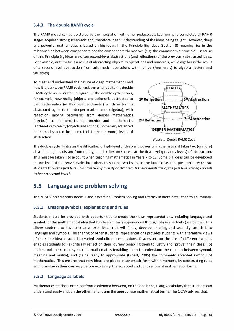
© QUT YuMi Deadly Centre 2016 5/03/2016 Big Ideas for Mathematics Page 63
5.4.3 The double RAMR cycle
The RAMR model can be bolstered by the integration with other pedagogies. Learners who completed all RAMR stages acquired strong schematic and, therefore, deep understanding of the ideas being taught. However, deep and powerful mathematics is based on big ideas. In the Principle Big Ideas (Section 3) meaning lies in the relationships between components not the components themselves (e.g. the commutative principle). Because of this, Principle Big Ideas are often second-level abstractions (and reflections) of the previously abstracted ideas. For example, arithmetic is a result of abstracting objects to operations and numerals, while algebra is the result of a second-level abstraction from arithmetic (operations with numbers/numerals) to algebra (letters and variables).
To meet and understand the nature of deep mathematics and how it is learnt, the RAMR cycle has been extended to the double RAMR cycle as illustrated in Figure …. The double cycle shows, for example, how reality (objects and actions) is abstracted to the mathematics (in this case, arithmetic) which in turn is abstracted again to the deeper mathematics (algebra), with reflection moving backwards from deeper mathematics (algebra) to mathematics (arithmetic) and mathematics (arithmetic) to reality (objects and actions). Some very advanced mathematics could be a result of three (or more) levels of abstraction.
The double cycle illustrates the difficulties of high-level or deep and powerful mathematics: it takes two (or more) abstractions; it is distant from reality; and it relies on success at the first level (previous levels) of abstraction. This must be taken into account when teaching mathematics in Years 7 to 12. Some big ideas can be developed in one level of the RAMR cycle, but others may need two levels. In the latter case, the questions are: Do the students know the first level? Has this been properly abstracted? Is their knowledge of the first level strong enough to bear a second level?
5.5 Language and problem solving
The YDM Supplementary Books 2 and 3 examine Problem Solving and Literacy in more detail than this summary.
5.5.1 Creating symbols, explanations and rules
Students should be provided with opportunities to create their own representations, including language and symbols of the mathematical idea that has been initially experienced through physical activity (see below). This allows students to have a creative experience that will firstly, develop meaning and secondly, attach it to language and symbols. The sharing of other students’ representations provides students with alternative views of the same idea attached to varied symbolic representations. Discussions on the use of different symbols enables students to: (a) critically reflect on their journey (enabling them to justify and “prove” their ideas); (b) understand the role of symbols in mathematics (enabling them to understand the relation between symbol, meaning and reality); and (c) be ready to appropriate (Ernest, 2005) the commonly accepted symbols of mathematics. This ensures that new ideas are placed in schematic form within memory, by constructing rules and formulae in their own way before explaining the accepted and concise formal mathematics forms.
5.5.2 Language as labels
Mathematics teachers often confront a dilemma between, on the one hand, using vocabulary that students can understand easily and, on the other hand, using the appropriate mathematical terms. The QCAA advises that:
Figure … Double RAMR Cycle
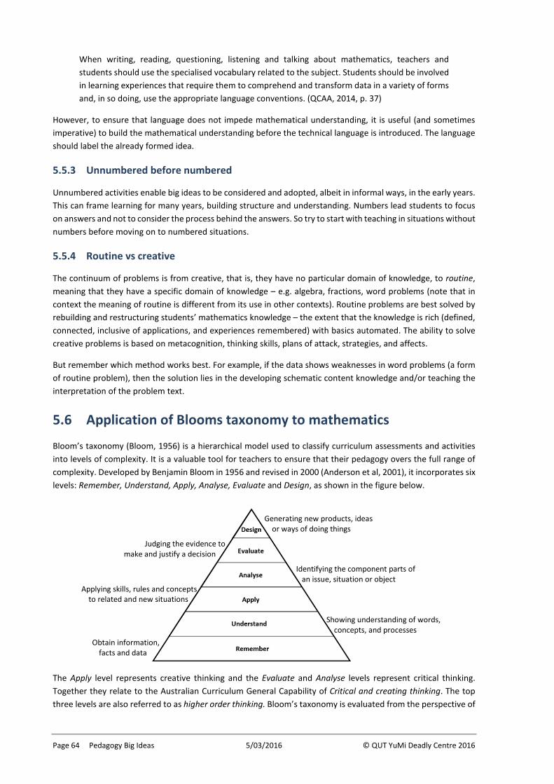
Page 64 Pedagogy Big Ideas 5/03/2016 © QUT YuMi Deadly Centre 2016
When writing, reading, questioning, listening and talking about mathematics, teachers and students should use the specialised vocabulary related to the subject. Students should be involved in learning experiences that require them to comprehend and transform data in a variety of forms and, in so doing, use the appropriate language conventions. (QCAA, 2014, p. 37)
However, to ensure that language does not impede mathematical understanding, it is useful (and sometimes imperative) to build the mathematical understanding before the technical language is introduced. The language should label the already formed idea.
5.5.3 Unnumbered before numbered
Unnumbered activities enable big ideas to be considered and adopted, albeit in informal ways, in the early years. This can frame learning for many years, building structure and understanding. Numbers lead students to focus on answers and not to consider the process behind the answers. So try to start with teaching in situations without numbers before moving on to numbered situations.
5.5.4 Routine vs creative
The continuum of problems is from creative, that is, they have no particular domain of knowledge, to routine, meaning that they have a specific domain of knowledge – e.g. algebra, fractions, word problems (note that in context the meaning of routine is different from its use in other contexts). Routine problems are best solved by rebuilding and restructuring students’ mathematics knowledge – the extent that the knowledge is rich (defined, connected, inclusive of applications, and experiences remembered) with basics automated. The ability to solve creative problems is based on metacognition, thinking skills, plans of attack, strategies, and affects.
But remember which method works best. For example, if the data shows weaknesses in word problems (a form of routine problem), then the solution lies in the developing schematic content knowledge and/or teaching the interpretation of the problem text.
5.6 Application of Blooms taxonomy to mathematics
Bloom’s taxonomy (Bloom, 1956) is a hierarchical model used to classify curriculum assessments and activities into levels of complexity. It is a valuable tool for teachers to ensure that their pedagogy overs the full range of complexity. Developed by Benjamin Bloom in 1956 and revised in 2000 (Anderson et al, 2001), it incorporates six levels: Remember, Understand, Apply, Analyse, Evaluate and Design, as shown in the figure below.
The Apply level represents creative thinking and the Evaluate and Analyse levels represent critical thinking. Together they relate to the Australian Curriculum General Capability of Critical and creating thinking. The top three levels are also referred to as higher order thinking. Bloom’s taxonomy is evaluated from the perspective of
Generating new products, ideas or ways of doing things
Judging the evidence to make and justify a decision
Showing understanding of words, concepts, and processes
Identifying the component parts of an issue, situation or object
Obtain information, facts and data
Applying skills, rules and concepts to related and new situations
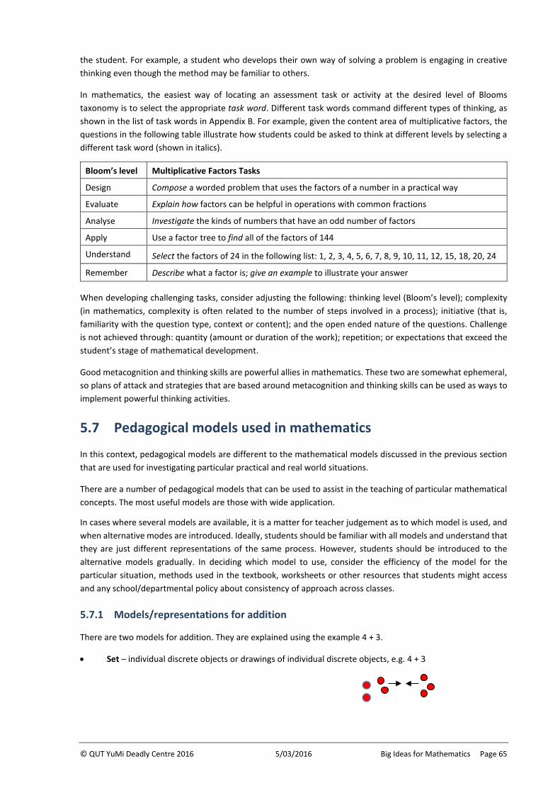
© QUT YuMi Deadly Centre 2016 5/03/2016 Big Ideas for Mathematics Page 65
the student. For example, a student who develops their own way of solving a problem is engaging in creative thinking even though the method may be familiar to others.
In mathematics, the easiest way of locating an assessment task or activity at the desired level of Blooms taxonomy is to select the appropriate task word. Different task words command different types of thinking, as shown in the list of task words in Appendix B. For example, given the content area of multiplicative factors, the questions in the following table illustrate how students could be asked to think at different levels by selecting a different task word (shown in italics).
Bloom’s level Multiplicative Factors Tasks
Design Compose a worded problem that uses the factors of a number in a practical way
Evaluate Explain how factors can be helpful in operations with common fractions
Analyse Investigate the kinds of numbers that have an odd number of factors
Apply Use a factor tree to find all of the factors of 144
Understand Select the factors of 24 in the following list: 1, 2, 3, 4, 5, 6, 7, 8, 9, 10, 11, 12, 15, 18, 20, 24
Remember Describe what a factor is; give an example to illustrate your answer
When developing challenging tasks, consider adjusting the following: thinking level (Bloom’s level); complexity (in mathematics, complexity is often related to the number of steps involved in a process); initiative (that is, familiarity with the question type, context or content); and the open ended nature of the questions. Challenge is not achieved through: quantity (amount or duration of the work); repetition; or expectations that exceed the student’s stage of mathematical development.
Good metacognition and thinking skills are powerful allies in mathematics. These two are somewhat ephemeral, so plans of attack and strategies that are based around metacognition and thinking skills can be used as ways to implement powerful thinking activities.
5.7 Pedagogical models used in mathematics
In this context, pedagogical models are different to the mathematical models discussed in the previous section that are used for investigating particular practical and real world situations.
There are a number of pedagogical models that can be used to assist in the teaching of particular mathematical concepts. The most useful models are those with wide application.
In cases where several models are available, it is a matter for teacher judgement as to which model is used, and when alternative modes are introduced. Ideally, students should be familiar with all models and understand that they are just different representations of the same process. However, students should be introduced to the alternative models gradually. In deciding which model to use, consider the efficiency of the model for the particular situation, methods used in the textbook, worksheets or other resources that students might access and any school/departmental policy about consistency of approach across classes.
5.7.1 Models/representations for addition
There are two models for addition. They are explained using the example 4 + 3.
• Set – individual discrete objects or drawings of individual discrete objects, e.g. 4 + 3
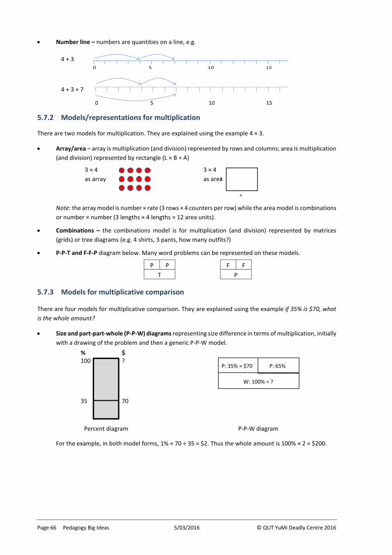
Page 66 Pedagogy Big Ideas 5/03/2016 © QUT YuMi Deadly Centre 2016
3
4
• Number line – numbers are quantities on a line, e.g.
4 + 3
4 + 3 = 7
5.7.2 Models/representations for multiplication
There are two models for multiplication. They are explained using the example 4 × 3.
• Array/area – array is multiplication (and division) represented by rows and columns; area is multiplication (and division) represented by rectangle (L × B = A)
3 × 4 3 × 4 as array as area
Note: the array model is number × rate (3 rows × 4 counters per row) while the area model is combinations or number × number (3 lengths × 4 lengths = 12 area units).
• Combinations – the combinations model is for multiplication (and division) represented by matrices (grids) or tree diagrams (e.g. 4 shirts, 3 pants, how many outfits?)
• P-P-T and F-F-P diagram below. Many word problems can be represented on these models.
5.7.3 Models for multiplicative comparison
There are four models for multiplicative comparison. They are explained using the example if 35% is $70, what is the whole amount?
• Size and part-part-whole (P-P-W) diagrams representing size difference in terms of multiplication, initially with a drawing of the problem and then a generic P-P-W model.
Percent diagram P-P-W diagram
For the example, in both model forms, 1% = 70 ÷ 35 = $2. Thus the whole amount is 100% × 2 = $200.
P P T
F F P
0 105 15
0 105 15
P: 35% = $70 P: 65%
W: 100% = ?
% 100 35
$ ? 70
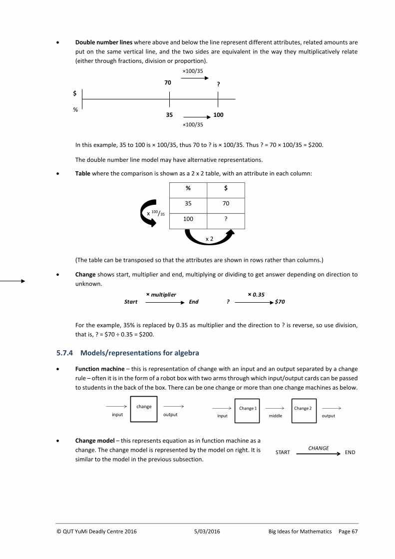
© QUT YuMi Deadly Centre 2016 5/03/2016 Big Ideas for Mathematics Page 67
• Double number lines where above and below the line represent different attributes, related amounts are put on the same vertical line, and the two sides are equivalent in the way they multiplicatively relate (either through fractions, division or proportion).
In this example, 35 to 100 is × 100/35, thus 70 to ? is × 100/35. Thus ? = 70 × 100/35 = $200.
The double number line model may have alternative representations.
• Table where the comparison is shown as a 2 x 2 table, with an attribute in each column:
% $
35 70
100 ?
(The table can be transposed so that the attributes are shown in rows rather than columns.)
• Change shows start, multiplier and end, multiplying or dividing to get answer depending on direction to unknown.
For the example, 35% is replaced by 0.35 as multiplier and the direction to ? is reverse, so use division, that is, ? = $70 ÷ 0.35 = $200.
5.7.4 Models/representations for algebra
• Function machine – this is representation of change with an input and an output separated by a change rule – often it is in the form of a robot box with two arms through which input/output cards can be passed to students in the back of the box. There can be one change or more than one change machines as below.
• Change model – this represents equation as in function machine as a change. The change model is represented by the model on right. It is similar to the model in the previous subsection.
× multiplierEndStart
× 0.35$70?
$ %
×100/35
35 100
×100/35
? 70
middleChange 1
input outputChange 2
outputchange
input
x 2
x 100/35
START ENDCHANGE
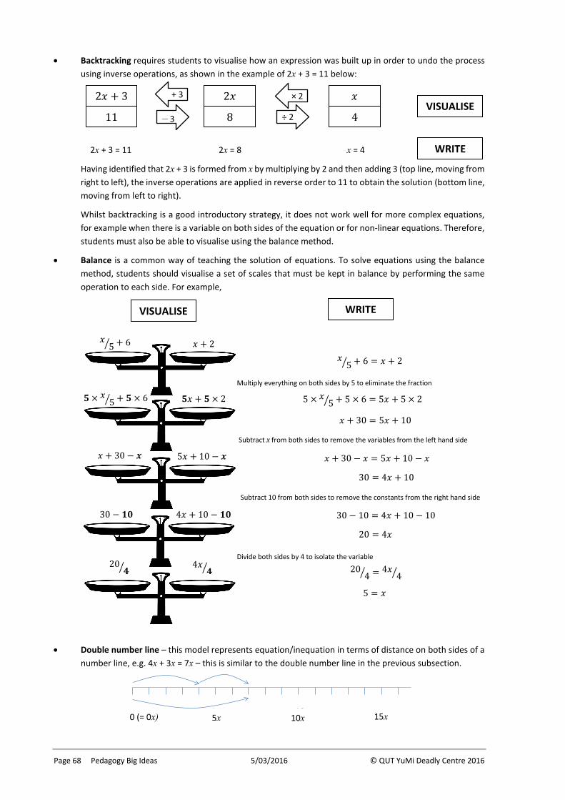
Page 68 Pedagogy Big Ideas 5/03/2016 © QUT YuMi Deadly Centre 2016
• Backtracking requires students to visualise how an expression was built up in order to undo the process using inverse operations, as shown in the example of 2x + 3 = 11 below:
2x + 3 = 11 2x = 8 x = 4
Having identified that 2x + 3 is formed from x by multiplying by 2 and then adding 3 (top line, moving from right to left), the inverse operations are applied in reverse order to 11 to obtain the solution (bottom line, moving from left to right).
Whilst backtracking is a good introductory strategy, it does not work well for more complex equations, for example when there is a variable on both sides of the equation or for non-linear equations. Therefore, students must also be able to visualise using the balance method.
• Balance is a common way of teaching the solution of equations. To solve equations using the balance method, students should visualise a set of scales that must be kept in balance by performing the same operation to each side. For example,
𝑥𝑥 5� + 6 = 𝑥𝑥 + 2
•
5 × 𝑥𝑥5� + 5 × 6 = 5𝑥𝑥 + 5 × 2
𝑥𝑥 + 30 = 5𝑥𝑥 + 10
•
𝑥𝑥 + 30 − 𝑥𝑥 = 5𝑥𝑥 + 10 − 𝑥𝑥
30 = 4𝑥𝑥 + 10
•
30 − 10 = 4𝑥𝑥 + 10 − 10
20 = 4𝑥𝑥
•
204� = 4𝑥𝑥
4�
5 = 𝑥𝑥
• Double number line – this model represents equation/inequation in terms of distance on both sides of a number line, e.g. 4x + 3x = 7x – this is similar to the double number line in the previous subsection.
0 105 15
WRITE
2𝑥𝑥 + 3
11
2𝑥𝑥
8
𝑥𝑥
4
× 2 + 3
– 3 ÷ 2 VISUALISE
𝑥𝑥5� + 6 𝑥𝑥 + 2
𝟓𝟓𝑥𝑥 + 𝟓𝟓 × 2 𝟓𝟓 × 𝑥𝑥5� + 𝟓𝟓 × 6
𝑥𝑥 + 30 − 𝒙𝒙 5𝑥𝑥 + 10 − 𝒙𝒙
30 − 𝟏𝟏𝟏𝟏 4𝑥𝑥 + 10 − 𝟏𝟏𝟏𝟏
20𝟒𝟒� 4𝑥𝑥
𝟒𝟒�
Multiply everything on both sides by 5 to eliminate the fraction
Subtract x from both sides to remove the variables from the left hand side
Subtract 10 from both sides to remove the constants from the right hand side
Divide both sides by 4 to isolate the variable
VISUALISE WRITE
0 (= 0x) 5x 10x 15x
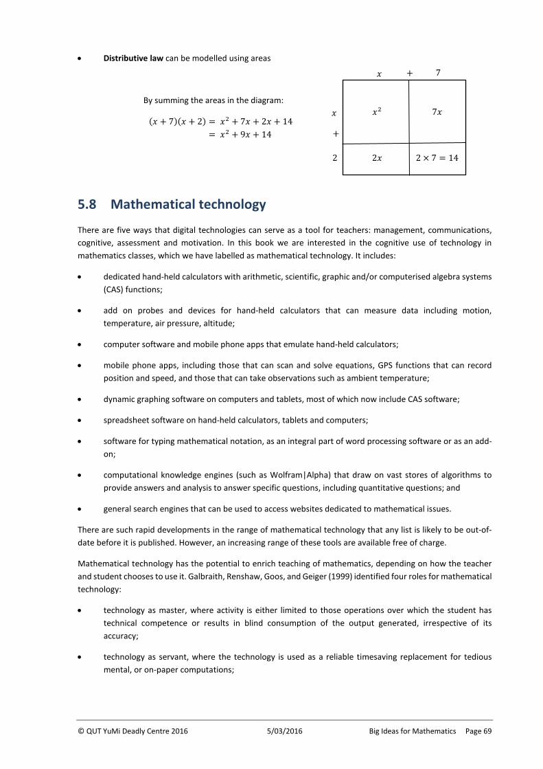
© QUT YuMi Deadly Centre 2016 5/03/2016 Big Ideas for Mathematics Page 69
• Distributive law can be modelled using areas
By summing the areas in the diagram:
(𝑥𝑥 + 7)(𝑥𝑥 + 2) = 𝑥𝑥2 + 7𝑥𝑥 + 2𝑥𝑥 + 14 = 𝑥𝑥2 + 9𝑥𝑥 + 14
5.8 Mathematical technology
There are five ways that digital technologies can serve as a tool for teachers: management, communications, cognitive, assessment and motivation. In this book we are interested in the cognitive use of technology in mathematics classes, which we have labelled as mathematical technology. It includes:
• dedicated hand-held calculators with arithmetic, scientific, graphic and/or computerised algebra systems (CAS) functions;
• add on probes and devices for hand-held calculators that can measure data including motion, temperature, air pressure, altitude;
• computer software and mobile phone apps that emulate hand-held calculators;
• mobile phone apps, including those that can scan and solve equations, GPS functions that can record position and speed, and those that can take observations such as ambient temperature;
• dynamic graphing software on computers and tablets, most of which now include CAS software;
• spreadsheet software on hand-held calculators, tablets and computers;
• software for typing mathematical notation, as an integral part of word processing software or as an add-on;
• computational knowledge engines (such as Wolfram|Alpha) that draw on vast stores of algorithms to provide answers and analysis to answer specific questions, including quantitative questions; and
• general search engines that can be used to access websites dedicated to mathematical issues.
There are such rapid developments in the range of mathematical technology that any list is likely to be out-of-date before it is published. However, an increasing range of these tools are available free of charge.
Mathematical technology has the potential to enrich teaching of mathematics, depending on how the teacher and student chooses to use it. Galbraith, Renshaw, Goos, and Geiger (1999) identified four roles for mathematical technology:
• technology as master, where activity is either limited to those operations over which the student has technical competence or results in blind consumption of the output generated, irrespective of its accuracy;
• technology as servant, where the technology is used as a reliable timesaving replacement for tedious mental, or on-paper computations;
𝑥𝑥2
𝑥𝑥 7
2
7𝑥𝑥
2𝑥𝑥 2 × 7 = 14
𝑥𝑥
+
+
Page 70 Pedagogy Big Ideas 5/03/2016 © QUT YuMi Deadly Centre 2016
• technology as partner, where the technology becomes “a friend to go exploring with, rather than merely a producer of results” (p. 225) and where the student understands that the process is more than just seeking a required result; and
• technology as extension of self, where the technology become an essential part of the student’s toolkit, along with mathematical knowledge, mental processes and on-paper skills.
More recently, and reflecting the development of new mathematical technologies, Dick and Hollebrands (2011) classified them as conveyance technologies (for presenting, communicating and sharing) and mathematical action technologies (that perform mathematical tasks). Sherman (2014) classified technology as amplifiers of mental activity (performing tedious tasks) or as a potential reorganizer of mental activity that shifted the focus of a student’s mathematical thinking from “drawing and measuring to looking for patterns and making and testing conjectures” (p. 223).
If mathematical technology is used only in the master/servant or amplifier roles, the full potential of the technology as a pedagogical tool is unlikely to be realised, to the disadvantage of students. Mathematical technology should be seen as a support for higher order thinking, that is, in the partner/extension of self, or reorganiser roles.
One thing to be avoided is the black box use of technology (Buchberger, 1989) such as using a regression tool to fit a curve to a data set, without any understanding of the regression process. This is often the case when the mathematical technology is regarded as a means to an end. Students are directed to a model through a scripted button-pushing recipe with little understanding. It often results in the selection of an inappropriate algebraic model that provides the closest fit to the data but ignores the underlying mathematical relationship. In the paper boxes examples, volume is the relevant mathematical relationship, suggesting that a cubic function would be the most appropriate, even though the technology might suggest that higher degree polynomials provide a better fit to the data.
The vast range of mathematical technology makes it difficult for a teacher to become an expert in all areas. However, all teachers should be familiar with the range of mathematical technologies available and be open to the possibility of using some of them as a tool to support their teaching of mathematics.
A supplementary YuMi Deadly book is currently being developed on the classroom use of mathematical technology.
© QUT YuMi Deadly Centre 2016 5/03/2016 Big Ideas for Mathematics Page 71
6 Superstructures: The convergence of big ideas
Mathematics is a comprehensive and interconnected body of knowledge. Because it is a network of ideas, it does not easily lend itself to a partitioning into topics or big ideas. Regardless of how the partitioning is done, there will always be connections to other parts of mathematics. As students mature mathematically, these connections become more apparent. In recognition of this, the discussion of the big ideas in this book also identifies the connections to other big ideas.
6.1 Concept maps
It is important that students understand that mathematics is a network of ideas. This is achieved gradually as students progress in their study of mathematics. For example, in the early years there may appear to be little to connect arithmetic operations and plane shapes. However, when students are introduced to the concept of area, which draws on understandings of both multiplication and squares, they should see the first of many connections between the two big ideas. As they continue in the study of mathematics, the teacher should draw students’ attention to these connections as they arise.
By the upper primary years, students should be able to illustrate their understanding of the connections between big ideas using a concept (or mind) map. As students prepare their own mathematical concept maps (not copying the teacher’s concept map), and add to them as they encounter new mathematical concepts, they reveal their growing understanding of the network of mathematical ideas. The act of preparing concept maps serves to emphasise connections between mathematical ideas. Initially the concept map may be of a radial design, with a central idea connected to other ideas like petals on a flower. However, as they start to see the connections between the “petals”, the concept maps become more complex.
Students’ concept maps can be an important diagnostic tool for teachers. The inclusion of some connections and omission of others reveal much about students’ thinking. They can point to areas where teacher intervention may be needed to make explicit links between, or even reteach, some concepts. As concept maps depend on understanding, rather than skills, they can help to identify those students with a sophisticated understanding of mathematics who may benefit from more challenging activities.
There is no single “correct” concept map. Different people will prepare different concept maps, depending on their own mathematical understandings (a person who ceased mathematical studies when they left school will produce a different map from an engineer), personal priorities (a surveyor, working every day with trigonometry, is likely to prepare a different mathematical concept map to an accountant); and age (a primary teacher is likely to develop a different concept map from a secondary mathematics teacher). This is reflected in a review of the academic literature (Carter, 2016) where little agreement was found on what constituted the big ideas of mathematics.
6.2 Pre-requisite knowledge and skills
Some mathematical concepts rely on pre-requisite knowledge. For example, calculus is a higher level application of mathematics that draws together several conceptual big ideas, including infiniteness (limits), number (measurement), multiplication (rates), shapes (area), and patterns and functions (functions and gradients) and also the principle of an inverse. The large number of connections demonstrates the extent of the knowledge that students must have mastered before they are ready for the study of calculus (explaining why it is taught in the upper secondary years). It also provides opportunities for students to connect the big ideas learnt previously.
Page 72 Superstructures: The convergence of big ideas5/03/2016 © QUT YuMi Deadly Centre 2016
If teachers can identify the big ideas that underpin a concept, they know the knowledge and skills that students must possess before the new concept is introduced. It can inform the content of a pre-test, if used, and the need to refresh past content before introducing the new work.
6.3 Superstructures
Often there appear to be inconsistencies in parts of mathematics. For example, addition and subtraction have important differences: (a) subtraction has an inverse relation for the second number (increasing second number for subtraction makes answer smaller), but this is not true for addition; and (b) subtraction is different for compensation (we have to increase both numbers for a subtraction to remain the same, whilst we have to do the opposite for addition). As this can be confusing for students, teachers often try to help by presenting addition and subtraction as different operations. However, the problem can be overcome by building superstructures (Cooper & Warren, 2011) that take account of these conflicts. When it is understood that addition and subtraction are inverses, then it is clear they should operate oppositely, making it reasonable that they act differently. This understanding also helps to understand that –(–4) = +4.
The idea of superstructures can assist in determining the sequencing of topics. For example, it is more effective for later Year levels to teach functional thinking before equivalence and equations. This is because the understanding of functions builds a strong superstructure around the inverse and identity principles which: (a) assists the solution of linear equations with an unknown; and (b) prevents conflict between inverse and balance, and the development of compound difficulties in the solution process
6.4 Convergence of big ideas
As students reach the higher level of mathematics the big ideas should converge. For example, the idea of subtraction of a separate concept can be discarded when students learn that subtraction is viewed as adding the negative (that is, the inverse). The concepts of number and operations merge as students recognise that the numbers are the set upon which the operations are defined. It can be thought of as the roots of a tree, where a large number of small roots converge to a smaller number of larger roots, and eventually to a single tree trunk. The goal is that, as students mature mathematically, they will come to view mathematics as a comprehensive and interconnected body of knowledge.
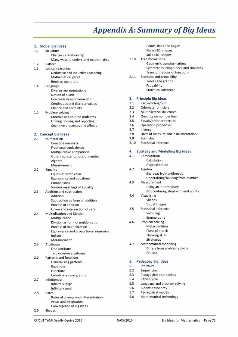
© QUT YuMi Deadly Centre 2016 5/03/2016 Big Ideas for Mathematics Page 73
Appendix A: Summary of Big Ideas
1. Global Big Ideas 1.1 Structure
Change vs relationship Many ways to understand mathematics
1.2 Pattern 1.3 Logical reasoning
Deductive and inductive reasoning Mathematical proof Boolean operators
1.4 Language Diverse representations Notion of a unit Exactness vs approximation Continuous and discrete values Chance and certainty
1.5 Problem solving Creative and routine problems Finding, solving and reporting Cognitive processes and affects
2. Concept Big Ideas 2.1 Numeration
Counting numbers Fractional equivalence Multiplicative comparison Other representations of number Algebra Measurement
2.2 Equality Equals as same value Equivalence and equations Comparisons Various meanings of equality
2.3 Addition and subtraction Addition Subtraction as form of addition Process of addition Union and intersection of sets
2.4 Multiplication and Division Multiplication Division as form of multiplication Process of multiplication Equivalence and proportional reasoning Indices Measurement
2.5 Attributes One attribute Two or more attributes
2.6 Patterns and functions Generalising patterns Equations Functions Coordinates and graphs
2.7 Infiniteness Infinitely large Infinitely small
2.8 Rates Rates of change and differentiation Areas and integration Convergence of big ideas
2.9 Shapes
Points, lines and angles Plane (2D) shapes Solid (3D) shapes
2.10 Transformations Geometric transformations Symmetries, congruence and similarity Transformations of functions
2.11 Statistics and probability Tables and graphs Probability Statistical inference
3. Principle Big Ideas 3.1 Part-whole-group 3.2 Odometer principle 3.3 Multiplicative structures 3.4 Quantity on number line 3.5 Equals/order properties 3.6 Operation properties 3.7 Inverse 3.8 Units of measure and instrumentation 3.9 Formulae 3.10 Statistical inference 4. Strategy and Modelling Big Ideas 4.1 Computation
Calculation Approximation
4.2 Algebra Big ideas from arithmetic Generalising/building from number
4.3 Measurement Using an intermediary Not confusing steps with end points
4.4 Visualising Shapes Visual images
4.5 Statistical inference Sampling Enumerating
4.6 Problem solving Metacognition Plans of attack Thinking skills Strategies
4.7 Mathematical modelling Differs from problem solving Process
5. Pedagogy Big Ideas 5.1 Structure 5.2 Sequencing 5.3 Pedagogical approaches 5.4 RAMR cycle 5.5 Language and problem solving 5.6 Blooms taxonomy 5.7 Pedagogical models 5.8 Mathematical technology
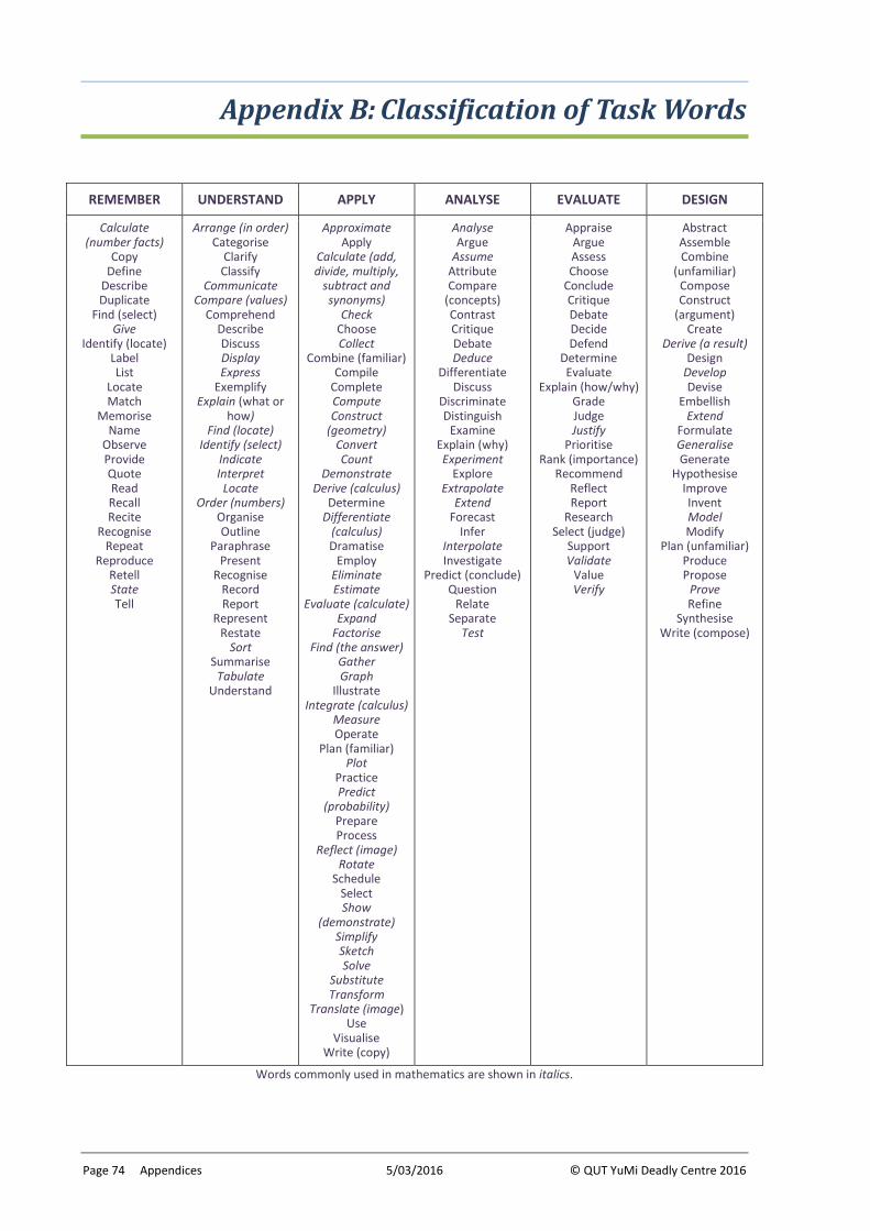
Page 74 Appendices 5/03/2016 © QUT YuMi Deadly Centre 2016
Appendix B: Classification of Task Words
REMEMBER UNDERSTAND APPLY ANALYSE EVALUATE DESIGN
Calculate (number facts)
Copy Define
Describe Duplicate
Find (select) Give
Identify (locate) Label List
Locate Match
Memorise Name
Observe Provide Quote Read Recall Recite
Recognise Repeat
Reproduce Retell State Tell
Arrange (in order) Categorise
Clarify Classify
Communicate Compare (values)
Comprehend Describe Discuss Display Express
Exemplify Explain (what or
how) Find (locate)
Identify (select) Indicate Interpret
Locate Order (numbers)
Organise Outline
Paraphrase Present
Recognise Record Report
Represent Restate
Sort Summarise
Tabulate Understand
Approximate Apply
Calculate (add, divide, multiply,
subtract and synonyms)
Check Choose Collect
Combine (familiar) Compile
Complete Compute Construct
(geometry) Convert Count
Demonstrate Derive (calculus)
Determine Differentiate
(calculus) Dramatise
Employ Eliminate Estimate
Evaluate (calculate) Expand
Factorise Find (the answer)
Gather Graph
Illustrate Integrate (calculus)
Measure Operate
Plan (familiar) Plot
Practice Predict
(probability) Prepare Process
Reflect (image) Rotate
Schedule Select Show
(demonstrate) Simplify Sketch Solve
Substitute Transform
Translate (image) Use
Visualise Write (copy)
Analyse Argue
Assume Attribute Compare
(concepts) Contrast Critique Debate Deduce
Differentiate Discuss
Discriminate Distinguish
Examine Explain (why) Experiment
Explore Extrapolate
Extend Forecast
Infer Interpolate Investigate
Predict (conclude) Question
Relate Separate
Test
Appraise Argue Assess Choose
Conclude Critique Debate Decide Defend
Determine Evaluate
Explain (how/why) Grade Judge Justify
Prioritise Rank (importance)
Recommend Reflect Report
Research Select (judge)
Support Validate
Value Verify
Abstract Assemble Combine
(unfamiliar) Compose Construct
(argument) Create
Derive (a result) Design
Develop Devise
Embellish Extend
Formulate Generalise Generate
Hypothesise Improve Invent Model Modify
Plan (unfamiliar) Produce Propose
Prove Refine
Synthesise Write (compose)
Words commonly used in mathematics are shown in italics.
© QUT YuMi Deadly Centre 2016 5/03/2016 Big Ideas for Mathematics Page 75
References
Anderson, L. W., Kratwohl, D. R., Airasian, P. W., Cruickshank, K., Mayer, R. E., Pintrich, P. R., Raths, J., & Wittrock, M. C. (2001). A taxonomy for learning, teaching, and assessing: A revision of Bloom's taxonomy of educational objectives. New York: Longman.
Box, G. E. P. (1976). Science and statistics. Journal of the American Statistical Association, 71(356), 791-799. doi: 10.2307/2286841
Bloom, B. S. (1956). Taxonomy of educational objectives: The classification of educational goals. London: Longman Group.
Buchberger, B. (1989). Why should students learn integration rules? RISC: Linz Technical Report, 89(7). Linz, Austria: Johannes Kepler University Austria.
Carter, M. (2011). Poster: Interpreting visual images. Brisbane, Qld: ITC Publications.
Carter, M. (2013). A picture is worth a thousand words: A cross-curricular approach to learning about visuals in STEM. International Journal of Engineering Education, 29(4), 1-7.
Charles, R. I. (2005). Big ideas and understandings as the foundation for elementary and middle school mathematics. Journal of Mathematics Education Leadership, 8(1), 9-24.
Cooper, T. J., & Warren, E. (2011). Years 2 to 6 students’ ability to generalise: Models, representations and theory for teaching and learning. In J. Cai & E. Knuth (eds.), Early algebraization: A global dialogue from multiple perspectives (pp. 187-214), Advances in Mathematics Education, DOI 10.1007/978-3-642-17735-4_12. Berlin Heidelberg: Springer-Verlag.
Davydov, V. (1995). The influence of L. S. Vygotsky on education theory, research, and practice. Educational Researcher, 24(3), 12-21.
Dick, T. P., & Hollebrands, K. F. (2011). Focus in high school mathematics: Technology to support reasoning and sense making. Reston, VA: National Council of Teachers of Mathematics.
Doyle, K. (2006). Organisational structure for mathematical modelling. Paper presented at the Identities, Cultures and Learning Spaces: 29th annual conference of the Mathematics Education Research Group of Australasia, Canberra.
English, L. D. (2008). Mathematical modelling: Linking mathematics, science, and the arts in the primary curriculum. Paper presented at the Proceedings of MACAS 2, Second International Symposium on Mathematics and Its Connections to the Arts and Sciences, Odense, Denmark.
Fisher, D., & Frey, N. (2008). Better learning through structured teaching. Alexandria, VA: Association for Supervision and Curriculum Development.
Galbraith, P., Renshaw, P., Goos, M., & Geiger, V. (1999). Technology, mathematics, and people: Interactions in a community of practice. Paper presented at the Making the Difference. Proceedings of the 22nd Annual Conference of the Mathematics Education Research Group of Australasia, Adelaide.
Jardine, D. W. (2006). Piaget and education primer. New York: Peter Lang Publishing, Inc.
Kuntze, S., Lerman, S., Murphy, B., Siller, H.-S., Kurz-Milcke, E., Winbourne, P., . . . Fuchs, K.-J. (2009). Awareness of big ideas in mathematics classrooms: ABCmaths progress report
Page 76 References 5/03/2016 © QUT YuMi Deadly Centre 2016
Lambdin, D. V. (2003). Benefits of teaching through problem solving. In F. K. Lester Jr (Ed.), Teaching mathematics through problem solving: Prekindergarten - Grade 6 (pp. 3-14). Reston, VA: National Council of Teachers of Mathematics.
Lesh, R. A., & Harel, G. (2003). Problem solving, modeling, and local conceptual development. Mathematical Thinking & Learning, 5(2/3), 157-189.
Lesh, R. A., Cramer, K., Doerr, H. M., Post, T., & Zawojewski, J. S. (2003). Model development sequences. In R. Lesh & H. M. Doerr (Eds.), Beyond constructivism: Models and modelling perspectives on mathematics problem solving, learning and teaching (pp. 35-58). Mahwah, NJ: Lawrence Erlbaum Associates.
Niss, M. (2006). The structure of mathematics and its influence on the learning process. In J. Maasz & W. Schloeglmann (Eds.), New mathematics education research and practice (pp. 51-62). Rotterdam, Netherlands: Sense Publishers. Piaget, J. W. F. (1977). The essential Piaget. New York: Basic Books Inc.
Öhlsson, S. (1993). Abstract schemas. Educational Psychologist, 28(1), 51-56.
Schifter, D., & Fosnot, C. T. (1993). Reconstructing mathematics education: Stories of teachers meeting the challenges of reform. New York, NY: Teachers College Press.
Siller, H.-S., & Kuntze, S. (2011). Modelling as a big idea in mathematics–Knowledge and views of pre-service and in-service teachers. Journal of Mathematical Modelling and Application, 1(6), 33-39.
Skemp, R. R. (1976). Relational understanding and instrumental understanding. Mathematics Teaching, 77, 20-26.
Stillman, G. A., Brown, J. P., & Geiger, V. (2015). Facilitating mathematisation in modelling by beginning modellers in secondary school. In G. A. Stillman, W. Blum & M. S. NBiembengut (Eds.), Mathematical Modelling in Education Research and Practice (pp. 93-103). Switzerland: Springer International Publishing.
Warren, E., & Cooper, T. J. (2007). Repeating patterns and multiplicative thinking: Analysis of classroom interactions with 9-year-old students that support the transition from the known to the novel. The Journal of Classroom Interaction, 41/42(2/1), 7-17.

© 2016 Queensland University of Technology through the YuMi Deadly Centre
Faculty of Education School of Curriculum
S Block, Room 404 Victoria Park Road
KELVIN GROVE QLD 4059 CRICOS No. 00213J
Phone: +61 7 3138 0035 Fax: +61 7 3138 3985
Email: [email protected] Website: http://ydc.qut.edu.au
Prep
to Y
ear 1
2: S
upp
lem
enta
ry R
esou
rce
1 –
Big
Idea
s of
Mat
hem
atic
s