Binary Outcomes Logistic Regression (Chapter 6)wguan/class/PUBH7402/notes/le… · · 2015-03-10Binary Outcomes – Logistic Regression (Chapter 6) • 2 by 2 tables • Odds ratio,

Binary Outcomes – Logistic Regression (Chapter 6)

• 2 by 2 tables

• Odds ratio, relative risk, risk difference

• Binomial regression - the logistic, log and linear link functions

• Categorical predictors - Continuous predictors

• Estimation by maximum likelihood

• Predicted probabilities

• Separation (Quasi-separation)

• Assessing model fit

A binary outcome example: WCGS

The Western Collaborative Group Study (WCGS): a large epidemiological

study of coronary heart disease (CHD).

Rosenman, R. H., Friedman, M., Straus, R., Wurm, M., Kositchek, R., Hahn, W. and

Werthessen, N. T. (1964). A predictive study of coronary heart disease: the western

collaborative group study. Journal of the American Medical Association, 189, 113–120.

Outcome - 0/1: an indicator of CHD status

Study question – Whether CHD rates are different between age groups (<50

vs. >=50)

2 by 2 tables (SAS) proc freq;

tables chd69 * bage_50/chisq cmh riskdiff;

run;

bage_50 chd69

Frequency‚

Percent ‚

Row Pct ‚

Col Pct ‚ 0‚ 1‚ Total

ƒƒƒƒƒƒƒƒƒˆƒƒƒƒƒƒƒƒˆƒƒƒƒƒƒƒƒˆ

0 ‚ 2104 ‚ 145 ‚ 2249

‚ 66.71 ‚ 4.60 ‚ 71.31

‚ 93.55 ‚ 6.45 ‚

‚ 72.63 ‚ 56.42 ‚


1 ‚ 793 ‚ 112 ‚ 905

‚ 25.14 ‚ 3.55 ‚ 28.69

‚ 87.62 ‚ 12.38 ‚

‚ 27.37 ‚ 43.58 ‚


Total 2897 257 3154

91.85 8.15 100.00

Statistics for Table of chd69 by bage_50

Statistic DF Value Prob

ƒƒƒƒƒƒƒƒƒƒƒƒƒƒƒƒƒƒƒƒƒƒƒƒƒƒƒƒƒƒƒƒƒƒƒƒƒƒƒƒƒƒƒƒƒƒƒƒƒƒƒƒƒƒ

Chi-Square 1 30.3033 <.0001

Likelihood Ratio Chi-Square 1 28.2000 <.0001

Continuity Adj. Chi-Square 1 29.5164 <.0001

Mantel-Haenszel Chi-Square 1 30.2937 <.0001

Phi Coefficient 0.0980

Contingency Coefficient 0.0976

Cramer's V 0.0980

Fisher's Exact Test

ƒƒƒƒƒƒƒƒƒƒƒƒƒƒƒƒƒƒƒƒƒƒƒƒƒƒƒƒƒƒƒƒƒƒ

Cell (1,1) Frequency (F) 2104

Left-sided Pr <= F 1.0000

Right-sided Pr >= F 7.622E-08

Table Probability (P) 3.993E-08

Two-sided Pr <= P 1.167E-07

2 by 2 tables (SAS): risk estimates Column 1 Risk Estimates

(Asymptotic) 95% (Exact) 95%

Risk ASE Confidence Limits Confidence Limits

ƒƒƒƒƒƒƒƒƒƒƒƒƒƒƒƒƒƒƒƒƒƒƒƒƒƒƒƒƒƒƒƒƒƒƒƒƒƒƒƒƒƒƒƒƒƒƒƒƒƒƒƒƒƒƒƒƒƒƒƒƒƒƒƒƒƒƒƒƒƒƒƒƒƒƒƒƒ

Row 1 0.9355 0.0052 0.9254 0.9457 0.9246 0.9453

Row 2 0.8762 0.0109 0.8548 0.8977 0.8530 0.8970

Total 0.9185 0.0049 0.9090 0.9281 0.9084 0.9278

Difference 0.0593 0.0121 0.0355 0.0830

Difference is (Row 1 - Row 2)

Column 2 Risk Estimates

(Asymptotic) 95% (Exact) 95%

Risk ASE Confidence Limits Confidence Limits

ƒƒƒƒƒƒƒƒƒƒƒƒƒƒƒƒƒƒƒƒƒƒƒƒƒƒƒƒƒƒƒƒƒƒƒƒƒƒƒƒƒƒƒƒƒƒƒƒƒƒƒƒƒƒƒƒƒƒƒƒƒƒƒƒƒƒƒƒƒƒƒƒƒƒƒƒƒ

Row 1 0.0645 0.0052 0.0543 0.0746 0.0547 0.0754

Row 2 0.1238 0.0109 0.1023 0.1452 0.1030 0.1470

Total 0.0815 0.0049 0.0719 0.0910 0.0722 0.0916

Difference -0.0593 0.0121 -0.0830 -0.0355

Difference is (Row 1 - Row 2)

• What is the rate of CHD in the younger group? What is the rate of CHD in

the older group?

• What is the difference in the rates of CHD between the two age groups?

2 by 2 tables (SAS): odds ratio, risk ratio Cochran-Mantel-Haenszel Statistics (Based on Table Scores)

Statistic Alternative Hypothesis DF Value Prob

ƒƒƒƒƒƒƒƒƒƒƒƒƒƒƒƒƒƒƒƒƒƒƒƒƒƒƒƒƒƒƒƒƒƒƒƒƒƒƒƒƒƒƒƒƒƒƒƒƒƒƒƒƒƒƒƒƒƒƒƒƒƒƒ

1 Nonzero Correlation 1 30.2937 <.0001

2 Row Mean Scores Differ 1 30.2937 <.0001

3 General Association 1 30.2937 <.0001

Estimates of the Common Relative Risk (Row1/Row2)

Type of Study Method Value 95% Confidence Limits

ƒƒƒƒƒƒƒƒƒƒƒƒƒƒƒƒƒƒƒƒƒƒƒƒƒƒƒƒƒƒƒƒƒƒƒƒƒƒƒƒƒƒƒƒƒƒƒƒƒƒƒƒƒƒƒƒƒƒƒƒƒƒƒƒƒƒƒƒƒƒƒƒƒ

Case-Control Mantel-Haenszel 2.0494 1.5806 2.6572

(Odds Ratio) Logit 2.0494 1.5806 2.6572

Cohort Mantel-Haenszel 1.0677 1.0394 1.0966

(Col1 Risk) Logit 1.0677 1.0394 1.0966

Cohort Mantel-Haenszel 0.5210 0.4122 0.6584

(Col2 Risk) Logit 0.5210 0.4122 0.6584

• How was 2.04945 calculated and what is it? How was 1.0677 calculated

and what is it? How was 0.521 calculated and what is it?

• What is the relative rate of CHD if a person is <50 as compared to >50?

• Is there a significant effect of age<50 over age>50?

2 by 2 tables (Stata) . tabulate bage_50 chd69, all exact row col

+-------------------+

| Key |

|-------------------|

| frequency |

| row percentage |

| column percentage |

+-------------------+

| chd69

bage_50 | 0 1 | Total

-----------+----------------------+----------

<50 | 2,104 145 | 2,249

| 93.55 6.45 | 100.00

| 72.63 56.42 | 71.31

-----------+----------------------+----------

>=50 | 793 112 | 905

| 87.62 12.38 | 100.00

| 27.37 43.58 | 28.69

-----------+----------------------+----------

Total | 2,897 257 | 3,154

| 91.85 8.15 | 100.00

| 100.00 100.00 | 100.00

Pearson chi2(1) = 30.3033 Pr = 0.000

likelihood-ratio chi2(1) = 28.2000 Pr = 0.000

Cramér's V = 0.0980

gamma = 0.3441 ASE = 0.058

Kendall's tau-b = 0.0980 ASE = 0.020

Fisher's exact = 0.000

1-sided Fisher's exact = 0.000

Stata - Epitab “Tables for epidemiologists” . cc chd69 bage_50 // for case-control study (to obtain estimated OR)

Proportion

| Exposed Unexposed | Total Exposed

-----------------+------------------------+------------------------

Cases | 112 145 | 257 0.4358

Controls | 793 2104 | 2897 0.2737

-----------------+------------------------+------------------------

Total | 905 2249 | 3154 0.2869

| Point estimate | [95% Conf. Interval]

|------------------------+------------------------

Odds ratio | 2.04938 | 1.565101 2.677467 (exact)

Attr. frac. ex. | .5120476 | .3610636 .6265127 (exact)

Attr. frac. pop | .2231492 |

+-------------------------------------------------

chi2(1) = 30.30 Pr>chi2 = 0.0000

. cs chd69 bage_50 // for cohort study (to obtain estimated RD & RR)

| bage_50 |

| Exposed Unexposed | Total

-----------------+------------------------+------------

Cases | 112 145 | 257

Noncases | 793 2104 | 2897

-----------------+------------------------+------------

Total | 905 2249 | 3154

Risk | .1237569 .0644731 | .0814838

| Point estimate | [95% Conf. Interval]

|------------------------+------------------------

Risk difference | .0592838 | .0355493 .0830183

Risk ratio | 1.919512 | 1.51876 2.42601

Attr. frac. ex. | .4790343 | .3415682 .5878006

Attr. frac. pop | .208762 |

+-------------------------------------------------

chi2(1) = 30.30 Pr>chi2 = 0.0000

Examining Odds Ratio, Risk Ratio and Risk Difference

We are interested in comparing: P(Outcome|Exposure 1) to

P(Outcome|Exposure 0). When the outcome is binary the probability is the

same as the expected value, hence if we let X represent exposure(s) of interest

(e.g. different treatments in a clinical trial, exposure to a carcinogen), we

compare E(Y |X = 1) = π1 to E(Y |X = 0) = π0. So π1 is probability of the event

given that X = 1 has occurred and π0 is the probability of the event given that X

= 0 has occurred.

The relative risk (risk ratio) or relative rate (rate or prevalence ratio) is:

RR = π1/π0

The risk (or rate or prevalence) difference, or absolute risk reduction is:

RD = π1 − π0

The odds ratio is:

OR = 𝜋1

1−𝜋1

𝜋0

1−𝜋0

Comparing OR, RR, and RD

This table considers scenarios when OR = 2

NOTE: odds = π/(1 − π), π = odds/(odds + 1)

• How does the RR differ from the OR across the different probabilities?

• How does the RD differ from the RR and OR?

Comparing OR, RR, and RD

NOTE: odds = π/(1 − π), π = odds/(odds + 1)

From Chaprter 10 of Harrell F (2001) Regression Modeling Strategies With applications

to linear models, logistic regression and survival analysis.

Figure 10.2: Absolute

benefit as a function of risk

of the event in a control

subject and the relative

effect (odds ratio) of the risk

factor. The odds ratios are

given for each curve.

Notes on OR, RR, and RD • Notice when the risk is small, the risk is well approximated by the odds and

hence the relative risk is well approximated by the odds ratio. This is why you

will hear the following: “The OR approximates the RR for rare diseases”.

• Notice that the risk difference becomes smaller as the rate is smaller, though the

relative risk (and odds ratio) can remain large.

• As the risk becomes common (> 10%), the OR greatly overestimates the RR.

• RR and RD are arguably more interpretable than OR, nevertheless the odds ratio

is ubiquitous in Public Health and Medicine despite the tendency for people to

interpret ORs as if they are RRs

• Recent push in medical and public health literature to get researchers to estimate

RR and RD (see more push for RD in medical literature with some Guidelines

for reporting only allowing RD rather than relative measures) rather than OR.

(e.g. Spiegelman, D. und Hertzmark, Easy SAS Calculations for Risk or

Prevalence Ratios and Differences, American Journal of Epidemiology, 2005,

162, 199-205.)

• NOTE: If data were collected from a case control study, then we cannot estimate

risk (or risk ratios) from the data without some auxiliary information about

overall prevalence in the population. But we can still estimate odds and hence

odds ratios.

2 by n tables . tabulate agec chd69, all exact row col

| chd69

agec | 0 1 | Total

-----------+----------------------+----------

35-40 | 512 31 | 543

| 94.29 5.71 | 100.00

| 17.67 12.06 | 17.22

-----------+----------------------+----------

41-45 | 1,036 55 | 1,091

| 94.96 5.04 | 100.00

| 35.76 21.40 | 34.59

-----------+----------------------+----------

46-50 | 680 70 | 750

| 90.67 9.33 | 100.00

| 23.47 27.24 | 23.78

-----------+----------------------+----------

51-55 | 463 65 | 528

| 87.69 12.31 | 100.00

| 15.98 25.29 | 16.74

-----------+----------------------+----------

56-60 | 206 36 | 242

| 85.12 14.88 | 100.00

| 7.11 14.01 | 7.67

-----------+----------------------+----------

Total | 2,897 257 | 3,154

| 91.85 8.15 | 100.00

| 100.00 100.00 | 100.00

Pearson chi2(4) = 46.6534 Pr = 0.000

likelihood-ratio chi2(4) = 44.9464 Pr = 0.000

Cramér's V = 0.1216

gamma = 0.2896 ASE = 0.045

Kendall's tau-b = 0.1012 ASE = 0.016

Fisher's exact = 0.000

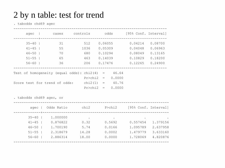
2 by n table: test for trend . tabodds chd69 agec

--------------------------------------------------------------------------

agec | cases controls odds [95% Conf. Interval]

------------+-------------------------------------------------------------

35-40 | 31 512 0.06055 0.04214 0.08700

41-45 | 55 1036 0.05309 0.04048 0.06963

46-50 | 70 680 0.10294 0.08049 0.13165

51-55 | 65 463 0.14039 0.10829 0.18200

56-60 | 36 206 0.17476 0.12265 0.24900

--------------------------------------------------------------------------

Test of homogeneity (equal odds): chi2(4) = 46.64

Pr>chi2 = 0.0000

Score test for trend of odds: chi2(1) = 40.76

Pr>chi2 = 0.0000

. tabodds chd69 agec, or

---------------------------------------------------------------------------

agec | Odds Ratio chi2 P>chi2 [95% Conf. Interval]

-------------+-------------------------------------------------------------

35-40 | 1.000000 . . . .

41-45 | 0.876822 0.32 0.5692 0.557454 1.379156

46-50 | 1.700190 5.74 0.0166 1.095789 2.637958

51-55 | 2.318679 14.28 0.0002 1.479779 3.633160

56-60 | 2.886314 18.00 0.0000 1.728069 4.820876

---------------------------------------------------------------------------

Modeling binary outcomes

Since Yi is 0-1 we can model it with a Binomial distribution with parameter πi.

So we have

and we can model E(Yi |Xi) = πi as a function of predictor variables Xi as

Modeling binary outcomes

Since πi is a probability, we require 0 ≤ πi ≤ 1. Hence, there are restrictions

on the acceptable values of Xi β (except for the logistic function)

Generalized linear modeling (GLM): Link functions

Given Yi |Xi ∼ Bin(1, πi) with E(Yi |Xi) = πi = g(Xβ), we want to rewrite the

relationship between π and Xβ so that Xβ is on a side by itself equal to a

nonlinear function of π. This inverse function is called the link function in

generalized linear modeling.

• The link function for the logistic is: 𝑙𝑜𝑔𝜋

1−𝜋= 𝑋𝛽

We call 𝑙𝑜𝑔𝜋

1−𝜋 the “logit link” and can write logit(π) = Xβ.

• The link function for the exponential is: log(π) = Xβ

which we simply call the “log link”.

• The link function for the π = Xβ is: I(π) = Xβ

which we call the “identity link” which means the relationship is already

linear and we don’t have to take any nonlinear function to make it linear.

Exponentiating coefficients in the Binomial-logistic model

results in an Odds Ratio

Consider what happens when X is increased by 1 unit...

So taking the difference we have,

Hence, if we take exp(β) we have odds ratio of Y given one unit increase in X.

Exponentiating coefficients in the Binomial-log model

results in a Relative Risk



Hence, if we take exp(β) we have relative risk of Y given one unit increase in

X.

Coefficients in the Binomial-identity model result in Risk

Differences



Binomial modeling in SAS ******* Logistic Binomial regression;

proc genmod data = wcgs descending;

class bage_50 (ref = "0")/param = ref;

model chd69 = bage_50/ dist = binomial link = logit type3;

estimate "log(OR) age>=50 vs. <50" bage_50 1/exp;

run;

proc logistic data = wcgs descending;


model chd69 = bage_50;

run;

******* Log binomial regression;



model chd69 = bage_50/ dist = binomial link = log type3;

estimate "log(RR) age>=50 vs. <50" bage_50 1/exp;

run;

******** Linear Binomial regression;



model chd69 = bage_50/ dist = binomial link = identity type3;

estimate "RD age>=50 vs. <50" bage_50 1;

run;

Details about syntax for Binomial modeling in SAS

A common feature of GENMOD and LOGISTIC is the descending option on

the PROC statement, which means for response data coded 0/1, SAS will

analyze the probability of a response of ’1’ rather than the default level of ’0’.

This option is an essential feature to recognize when interpreting the sign of

estimated coefficients because interpretation would be completely opposite.

Potential confusion between the two procedures can arise from the CLASS

statement. The defaults in the two procedures is different. To make them the

same, we use the /param = ref option which allows us to specify whichever

category we want to be the reference. By default Genmod would use the last

category and fix to 0, by default Logistic would use a coding that makes the

sum of the coefficients across categories = 0, which can lead to confusion when

testing individual parameters.

Binomial modeling in Stata: logit link . glm chd69 bage_50, family(binomial) link(logit)

Generalized linear models No. of obs = 3154

Optimization : ML Residual df = 3152

Scale parameter = 1

Deviance = 1753.043713 (1/df) Deviance = .5561687

Pearson = 3154 (1/df) Pearson = 1.000635

Variance function: V(u) = u*(1-u) [Bernoulli]

Link function : g(u) = ln(u/(1-u)) [Logit]

AIC = .5570842

Log likelihood = -876.5218566 BIC = -23640.81

------------------------------------------------------------------------------

| OIM

chd69 | Coef. Std. Err. z P>|z| [95% Conf. Interval]

-------------+----------------------------------------------------------------

bage_50 | .7175375 .1325196 5.41 0.000 .4578039 .9772711

_cons | -2.674862 .0858594 -31.15 0.000 -2.843143 -2.50658

------------------------------------------------------------------------------

. logistic chd69 bage_50

Logistic regression Number of obs = 3154

LR chi2(1) = 28.20

Prob > chi2 = 0.0000

Log likelihood = -876.52186 Pseudo R2 = 0.0158

------------------------------------------------------------------------------

chd69 | Odds Ratio Std. Err. z P>|z| [95% Conf. Interval]

-------------+----------------------------------------------------------------

bage_50 | 2.049379 .2715829 5.41 0.000 1.580598 2.657194

_cons | .0689163 .0059171 -31.15 0.000 .0582423 .0815466

------------------------------------------------------------------------------

Binomial modeling in Stata: log link . glm chd69 bage_50, family(binomial) link(log)



Scale parameter = 1




Link function : g(u) = ln(u) [Log]

AIC = .5570842


------------------------------------------------------------------------------

| OIM


-------------+----------------------------------------------------------------

bage_50 | .6520711 .1194802 5.46 0.000 .4178943 .8862479

_cons | -2.741507 .0803238 -34.13 0.000 -2.898939 -2.584075

------------------------------------------------------------------------------

. di exp(_b[bage_50]) // estimated RR

1.9195123

Note: match the estimated RR with previous output of 2 by 2 table.

Binomial modeling in Stata: identity link . glm chd69 bage_50, family(binomial) link(identity)



Scale parameter = 1




Link function : g(u) = u [Identity]

AIC = .5570842


------------------------------------------------------------------------------

| OIM


-------------+----------------------------------------------------------------

bage_50 | .0592838 .0121097 4.90 0.000 .0355493 .0830183

_cons | .0644731 .0051787 12.45 0.000 .054323 .0746232

------------------------------------------------------------------------------

Coefficients are the risk differences.

Note: match the estimated RD with previous output of 2 by 2 table.

Predicted probabilities . glm chd69 i.bage_50, family(binomial) link(logit)

. margins bage_50

------------------------------------------------------------------------------

| Delta-method

| Margin Std. Err. z P>|z| [95% Conf. Interval]

-------------+----------------------------------------------------------------

bage_50 |

0 | .0644731 .0051787 12.45 0.000 .054323 .0746232

1 | .1237569 .0109464 11.31 0.000 .1023023 .1452115

------------------------------------------------------------------------------

. glm chd69 i.bage_50, family(binomial) link(log)

. margins bage_50

------------------------------------------------------------------------------

| Delta-method


-------------+----------------------------------------------------------------

bage_50 |

0 | .0644731 .0051787 12.45 0.000 .054323 .0746232

1 | .1237569 .0109464 11.31 0.000 .1023023 .1452115

------------------------------------------------------------------------------

. glm chd69 i.bage_50, family(binomial) link(identity)

. margins bage_50

------------------------------------------------------------------------------

| Delta-method


-------------+----------------------------------------------------------------

bage_50 |

0 | .0644731 .0051787 12.45 0.000 .054323 .0746232

1 | .1237569 .0109464 11.31 0.000 .1023023 .1452115

------------------------------------------------------------------------------

Categorical predictor with >2 groups . glm chd69 i.agec, family(binomial) link(logit) eform



Scale parameter = 1





AIC = .553677


------------------------------------------------------------------------------

| OIM


-------------+----------------------------------------------------------------

agec |

1 | .8768215 .2025406 -0.57 0.569 .5575563 1.378903

2 | 1.70019 .3800504 2.37 0.018 1.097046 2.634935

3 | 2.318679 .5274963 3.70 0.000 1.484545 3.621494

4 | 2.886314 .7462298 4.10 0.000 1.738895 4.790864

|

_cons | .0605469 .0111989 -15.16 0.000 .0421358 .0870026

------------------------------------------------------------------------------

Note: match the estimated OR with previous output of 2 by n table.

Note: Try to avoid choosing the smallest group as the reference group (inflate

SE)

Aggregated binary outcomes: grouped data

With only categorical predictors it is possible to aggregate the data across all

possible combination of categories and input and analyze the data in aggregated

form - Bin(nk, πk).

Recall that the sum of n independent Bernoulli events from a trial with same

probability π leads to the Binomial(n, π) distribution. That is, if Yi ∼ Bin(1, πi)

where πi = πk for all i in some group k of size nk, then 𝑌𝑖𝑛𝑘𝑖=1 ~𝐵𝑖𝑛 𝑛𝑘 , 𝜋𝑖 .

Data in aggregated Binomial form can be modeled in both Proc Logistic and

Proc Genmod using the events/trials syntax in the model statement.

SAS: data aggregate;

input agegrp $ total totlechd;

cards;

<50 2249 145

>=50 905 112

;

proc genmod data = aggregate;

class agegrp(ref = "<50")/param = ref;;

model totlechd / total = agegrp / dist = binomial link = logit type3;

estimate "lnOR CG vs. SG" agegrp 1/exp;

run;

Stata: blogit totalchd total agegrp, or

Categorical/Continuous predictors

With categorical predictors and without any adjustment for other variables,

model fits (maximized log-likelihood & predicted probabilities) are the same

across 3 different link functions since the form does not really come into the

estimation (each category is its own dummy variable and hence can be

perfectly fit by any of the 3 functions). Basically, with a categorical predictor

and a dichotomous outcome, analysis mimic that for 2-way tables.

With a continuous predictor, the functional form matters and the different links

will result in different fits to the data. A continuous predictor is assumed to be

linearly related to the link function of the probability (for the identity link), but

this means it is nonlinearly related to the probability by the logistic function

(for the logit link) or the exponential function (for the log link).

Controlling for other variables: behavior pattern

The WCGS study measured a number of potential predictors of coronary heart

disease, including total serum cholesterol, diastolic and systolic blood pressure,

smoking, age, body size, and behavior pattern. Suppose we want to control for

potential confounding effect of behavior pattern (“A” vs “B”).

dibpat bage_50

Frequency‚

Percent ‚

Row Pct ‚



0 ‚ 1182 ‚ 383 ‚ 1565

‚ 37.48 ‚ 12.14 ‚ 49.62

‚ 75.53 ‚ 24.47 ‚

‚ 52.56 ‚ 42.32 ‚


1 ‚ 1067 ‚ 522 ‚ 1589

‚ 33.83 ‚ 16.55 ‚ 50.38

‚ 67.15 ‚ 32.85 ‚

‚ 47.44 ‚ 57.68 ‚


Total 2249 905 3154

71.31 28.69 100.00

Statistics for Table of dibpat by bage_50



Chi-Square 1 27.0485 <.0001






Cramer's V 0.0926

Behavior pattern vs. CHD

dibpat chd69

Frequency‚

Percent ‚

Row Pct ‚



0 ‚ 1486 ‚ 79 ‚ 1565

‚ 47.11 ‚ 2.50 ‚ 49.62

‚ 94.95 ‚ 5.05 ‚

‚ 51.29 ‚ 30.74 ‚


1 ‚ 1411 ‚ 178 ‚ 1589

‚ 44.74 ‚ 5.64 ‚ 50.38

‚ 88.80 ‚ 11.20 ‚

‚ 48.71 ‚ 69.26 ‚


Total 2897 257 3154

91.85 8.15 100.00

Statistics for Table of dibpat by chd69



Chi-Square 1 39.8975 <.0001






Cramer's V 0.1125

Stratification by behavior pattern

dibpat=0

bage_50 chd69

Frequency‚

Percent ‚

Row Pct ‚



0 ‚ 1132 ‚ 50 ‚ 1182

‚ 72.33 ‚ 3.19 ‚ 75.53

‚ 95.77 ‚ 4.23 ‚

‚ 76.18 ‚ 63.29 ‚


1 ‚ 354 ‚ 29 ‚ 383

‚ 22.62 ‚ 1.85 ‚ 24.47

‚ 92.43 ‚ 7.57 ‚

‚ 23.82 ‚ 36.71 ‚


Total 1486 79 1565

94.95 5.05 100.00

Chi-Square p-value = 0.0094

dibpat=1

bage_50 chd69

Frequency‚

Percent ‚

Row Pct ‚



0 ‚ 972 ‚ 95 ‚ 1067

‚ 61.17 ‚ 5.98 ‚ 67.15

‚ 91.10 ‚ 8.90 ‚

‚ 68.89 ‚ 53.37 ‚


1 ‚ 439 ‚ 83 ‚ 522

‚ 27.63 ‚ 5.22 ‚ 32.85

‚ 84.10 ‚ 15.90 ‚

‚ 31.11 ‚ 46.63 ‚


Total 1411 178 1589

88.80 11.20 100.00

Chi-Square p-value < 0.0001

Multiple predictors model: GLM . glm chd69 bage_50 dibpat, family(binomial) link(logit) eform



Scale parameter = 1


Pearson = 3157.01249 (1/df) Pearson = 1.001908



AIC = .5465198


------------------------------------------------------------------------------

| OIM


-------------+----------------------------------------------------------------

bage_50 | 1.909471 .2553643 4.84 0.000 1.469187 2.481699

dibpat | 2.249161 .3172902 5.75 0.000 1.705851 2.965513

_cons | .0437069 .0054894 -24.92 0.000 .0341698 .0559058

------------------------------------------------------------------------------

What is the interpretation of the estimated OR = 1.909?

How does the estimated OR change compared to the single predictor model?

Try to explain the direction of the change by the confounding/mediation effect.

Multiple predictors model: logistic regression . logistic chd69 bage_50 dibpat


LR chi2(2) = 63.52

Prob > chi2 = 0.0000


------------------------------------------------------------------------------


-------------+----------------------------------------------------------------

bage_50 | 1.909472 .2553643 4.84 0.000 1.469188 2.481699

dibpat | 2.24916 .3172901 5.75 0.000 1.705851 2.965513

_cons | .0437069 .0054894 -24.92 0.000 .0341698 .0559058

------------------------------------------------------------------------------

NOTE these results are identical to using the GLM function on the previous

page. Similar to the difference in SAS between using PROC LOGISTIC

versus PROC GENMOD.

Multiple predictors model: log link . glm chd69 bage_50 dibpat, family(binomial) link(log) eform



Scale parameter = 1


Pearson = 3153.822736 (1/df) Pearson = 1.000896


Link function : g(u) = ln(u) [Log]

AIC = .5465131


------------------------------------------------------------------------------

| OIM

chd69 | Risk Ratio Std. Err. z P>|z| [95% Conf. Interval]

-------------+----------------------------------------------------------------

bage_50 | 1.787009 .2131373 4.87 0.000 1.414502 2.257615

dibpat | 2.102816 .2747188 5.69 0.000 1.627786 2.716471

_cons | .0423275 .0050018 -26.76 0.000 .0335766 .0533592

------------------------------------------------------------------------------

What is the adjusted RR of having CHD for a person in the older age group?

How does the OR compare to the RR here?

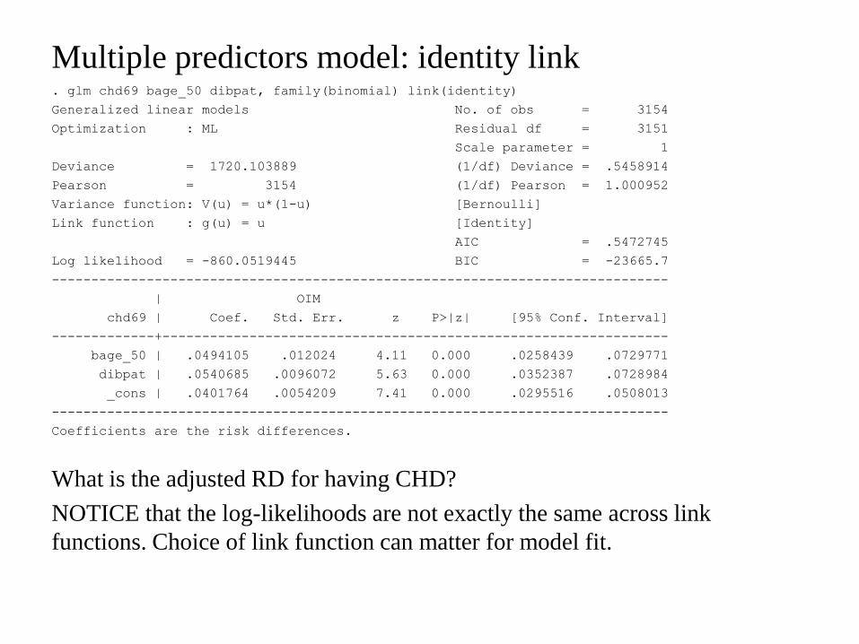
Multiple predictors model: identity link . glm chd69 bage_50 dibpat, family(binomial) link(identity)



Scale parameter = 1




Link function : g(u) = u [Identity]

AIC = .5472745


------------------------------------------------------------------------------

| OIM


-------------+----------------------------------------------------------------

bage_50 | .0494105 .012024 4.11 0.000 .0258439 .0729771

dibpat | .0540685 .0096072 5.63 0.000 .0352387 .0728984

_cons | .0401764 .0054209 7.41 0.000 .0295516 .0508013

------------------------------------------------------------------------------

Coefficients are the risk differences.

What is the adjusted RD for having CHD?

NOTICE that the log-likelihoods are not exactly the same across link

functions. Choice of link function can matter for model fit.

Predicted probabilities

After class: show how to calculate the predicted probability of CHD if a

person was in the <50 age group and was with behavior patter “B” using

the logit, log and identity models.

.05

.1.1

5

Pre

dic

ted P

rob

ab

ility

<50 >=50age group

raw proportion

logit link

log link

identity link

Predicted probabilities

Here are the predicted probabilities of CHD based on the fit of the 3 different

binomial regression models with main effects for age group and behavior

pattern: (verify your calculations)

dibpat bage_50 raw logit log identity 0 <50 .042301 .0418766 .0423275 .0401764

1 <50 .089035 .0895051 .0890069 .094245

0 >=50 .075718 .0770284 .0756396 .089587

1 >=50 .159004 .1580424 .1590562 .1436555

Using the numbers above, show how you can get the estimated ORs, RRs, and

RDs in the logit, log, and identity model results, respectively.

High birthweight example - a continuous predictor

How is a mother’s gestational weight gain and baseline weight status related to

the probability of the baby being born with a birthweight considered clinically

in the High range (i.e. > 4000 grams or > 8.8 pounds).

High birthweight versus mother’s baseline weight status

4 categories of baseline weight status: 1 underweight, 2 normal weight, 3

overweight, 4 obese.

Hight birthweight example: logistic regression (1) proc logistic data = birthwgt2 descending;

class c_baseline_bmi (ref = "2") /param = ref;

model hibwt = totalweightgain c_baseline_bmi/expb;

run;

Response Profile

Ordered Total

Value hibwt Frequency

1 1 260

2 0 1740

Probability modeled is hibwt=1.

Model Fit Statistics

Intercept

Intercept and

Criterion Only Covariates

AIC 1547.547 1440.462

SC 1553.148 1468.467

-2 Log L 1545.547 1430.462

Testing Global Null Hypothesis: BETA=0

Test Chi-Square DF Pr > ChiSq

Likelihood Ratio 115.0847 4 <.0001

Score 111.9801 4 <.0001

Wald 97.3858 4 <.0001

Hight birthweight example: logistic regression (2) Type 3 Analysis of Effects

Wald

Effect DF Chi-Square Pr > ChiSq

totalweightgain 1 59.3112 <.0001

c_baseline_bmi 3 61.4573 <.0001

Standard Wald

Parameter DF Estimate Error Chi-Square Pr > ChiSq Exp(Est)

Intercept 1 -3.5707 0.2190 265.8230 <.0001 0.028

totalweightgain 1 0.0406 0.00527 59.3112 <.0001 1.041

c_baseline_bmi 1 1 -1.7757 0.5944 8.9254 0.0028 0.169

c_baseline_bmi 3 1 0.7550 0.1886 16.0255 <.0001 2.128

c_baseline_bmi 4 1 1.0724 0.1613 44.1827 <.0001 2.922

Odds Ratio Estimates

Point 95% Wald

Effect Estimate Confidence Limits

totalweightgain 1.041 1.031 1.052

c_baseline_bmi 1 vs 2 0.169 0.053 0.543

c_baseline_bmi 3 vs 2 2.128 1.470 3.079

c_baseline_bmi 4 vs 2 2.922 2.130 4.009

• How many women had Hi birthweight babies?

• What is the test statistic value associated with the Hypothesis that there are No differences across baseline

bmi categories?

• What is the OR associated with a 10 pound higher gain in totalweightgain?

• How do we interpret the last OR estimate = 2.922? Is it stat sig?

Fitted values on the link scale and the probability scale

Recall the high birthweight example. We regressed high birthweight on both

mother’s total weight gain AND mother’s baseline BMI category.

logit(π) = -3.57+0.0405∗totwtgain−1.776∗underwt+0.755∗overwt+1.072∗obese

Compare the differences between what a change in the predictors means on the

two different scales.

Interpreting the intercept

logit(π) = -3.57+0.0405∗totwtgain−1.776∗underwt+0.755∗overwt+1.072∗obese

What does the intercept represent? Back transform it.

Intercept Term in Case-Control Study

• Case-control studies collect a fixed number of cases and controls, whose

ratio is typically different from population disease prevalence.

• Let Z indicate whether a subject is sampled or not. The probability of

sampling a case ρ1 = P(Z=1|Y=1), and the probability of sampling a control

ρ0 = P(Z=1|Y=0).

• Assume P(Y = 1 | x) follows the logistic model, and the sampling

probabilities does not depend on x. Then,

and

1

0

1| 1, 1|1| 1, (Bayes' theorem)

1| , |j

P Z y x P Y xP Y z x

P Z y j x P Y j x

1

0 1

exp1| 1,

exp

xP Y z x

x

1 0

*

logit 1| 1, logP Y z x x

x

Hight birthweight example: Stata output . logistic hibwt totalweightgain ib2.c_baseline_bmi

/* "ib2." tells Stata that bmi==2 is the reference(base) level */


LR chi2(4) = 115.08

Prob > chi2 = 0.0000


---------------------------------------------------------------------------------

hibwt | Odds Ratio Std. Err. z P>|z| [95% Conf. Interval]

----------------+----------------------------------------------------------------

totalweightgain | 1.041433 .0054899 7.70 0.000 1.030728 1.052248

|

c_baseline_bmi |

1 | .1693707 .1006664 -2.99 0.003 .052835 .5429432

3 | 2.127668 .4012924 4.00 0.000 1.47015 3.079259

4 | 2.922298 .4714581 6.65 0.000 2.130096 4.009128

|

_cons | .0281374 .0061622 -16.30 0.000 .0183176 .0432215

---------------------------------------------------------------------------------

old version:

. char c_baseline_bmi[omit] 2

. xi: logistic hibwt totalweightgain i.c_baseline_bmi

Estimation by Maximum Likelihood

Maximizing the likelihood

• This goal of maximizing the likelihood is accomplished using calculus

which provides tools for maximizing functions. The derivative of the log

likelihood is taken with respect to the parameter vector Θ and set equal to

0. The derivative of the log likelihood is called the score function.

• The maximum likelihood estimates are found by solving the score

function which will yield the values that maximize the likelihood assuming

the likelihood is unimodal. In general this solution must be found

numerically (no closed form).

• Problems can occur when likelihood function is multimodal (only find local

maximum rather than global maximum) or when the maximum is found

along the boundary of the parameter space.

• We use the hat notation, Θ , to indicate the MLEs of Θ.

• The second derivative of the log likelihood is called the information and is

used in creating standard errors.

The likelihood for logistic regression

Hypothesis testing from maximum likelihood theory

High birthweight example - Overall Model tests

The value of the Model Fit Statistics are only meaningful when they are

compared across models. By default SAS will compare the model with no

predictors (Intercept only) to the full model you have specified (Intercept and

Covariates). Here the model has totalwtgain (1 d.f.) and baseline BMI status (3

d.f).

Model Fit Statistics

Intercept

Intercept and

Criterion Only Covariates

AIC 1547.547 1440.462

SC 1553.148 1468.467

-2 Log L 1545.547 1430.462




Score 111.9801 4 <.0001

Wald 97.3858 4 <.0001

*. 1545.547-1430.462 = 115.085

The tests of global null hypothesis are like the overall model F-test in ANOVA

Confidence intervals - Wald or likelihood ratio based

• Wald tests are computationally faster than likelihood ratio test

• SAS and Stata create Wald confidence intervals by default. Estimate +-

1.96 * S.E.

– Adding the option CLodds = PL to the model statement in SAS will

provide the “profile likelihood confidence intervals”. These confidence

intervals based on the likelihood ratio test

• Hauck and Donner (1977) Wald’s test as applied to hypotheses in logit

analysis. Journal of the American Statistical Association, 72:851-863

notice that the Wald CI can be too large especially when there are strong

effects.

• LR confidence intervals considered better. With larger samples they will be

very similarly (asymptotically the same).

01

y

0 1 2x

Problem of Separation in Logistic Regression

• An identifiability problem that can arise in logistic regression, called

separation, occurs when a predictor or a combination of predictors are

perfectly aligned with the outcome such that y = 0 for ALL values of that

predictor beyond some point and y = 1 for ALL values of that predictor less

than some point.

• Often occurs in small or sparse samples with highly predictive covariates.

• Simples case is in the analysis of a 2 × 2 table with one zero cell count.

• For a continuous predictor, separation can be demonstrated by:

• For a categorical predictor separation means that in some category (or with

multiple predictors, in some combination of categories) all individuals in

that category either have a 1 or 0.

• Leads to non-convergence of the likelihood and/or infinite parameter

estimates.

Classical solution

Drop the predictor or somehow aggregate levels. Leave problematic predictors

in but only report results for predictors without separation problem.

Modern solution

See the website http://www.meduniwien.ac.at/msi/biometrie/programme/fl/

“Logistic regression using Firth’s bias reduction: a solution to the problem of

separation in logistic regression”. Heinze and Ploner, 2004 put together a SAS

MACRO (%fl) and also an R package (logistf()) that uses a penalized

maximum likelihood method to obtain estimates. In Stata, install user-written

command -firthlogit-.

Solutions to the problem of Separation

http://www.meduniwien.ac.at/msi/biometrie/programme/fl/

http://www.meduniwien.ac.at/msi/biometrie/programme/fl/

Summarizing predictive ability in logistic regression

. estat class, cutoff(.2)

Logistic model for hibwt

-------- True --------

Classified | D ~D | Total

-----------+--------------------------+-----------

+ | 89 239 | 328

- | 171 1501 | 1672

-----------+--------------------------+-----------

Total | 260 1740 | 2000

Classified + if predicted Pr(D) >= .2

True D defined as hibwt != 0

--------------------------------------------------

Sensitivity Pr( +| D) 34.23%

Specificity Pr( -|~D) 86.26%

Positive predictive value Pr( D| +) 27.13%

Negative predictive value Pr(~D| -) 89.77%

--------------------------------------------------

False + rate for true ~D Pr( +|~D) 13.74%

False - rate for true D Pr( -| D) 65.77%

False + rate for classified + Pr(~D| +) 72.87%

False - rate for classified - Pr( D| -) 10.23%

--------------------------------------------------

Correctly classified 79.50%

--------------------------------------------------

Classification table: Stata output

The LOGISTIC Procedure

Classification Table

Correct Incorrect Percentages

Prob Non- Non- Sensi- Speci- False False

Level Event Event Event Event Correct tivity ficity POS NEG

0.000 260 0 1740 0 13.0 100.0 0.0 87.0 .

0.020 259 110 1630 1 18.5 99.6 6.3 86.3 0.9

0.040 258 163 1577 2 21.1 99.2 9.4 85.9 1.2

0.060 251 311 1429 9 28.1 96.5 17.9 85.1 2.8

0.080 239 534 1206 21 38.7 91.9 30.7 83.5 3.8

0.100 208 805 935 52 50.7 80.0 46.3 81.8 6.1

0.120 180 1020 720 80 60.0 69.2 58.6 80.0 7.3

0.140 157 1183 557 103 67.0 60.4 68.0 78.0 8.0

0.160 130 1327 413 130 72.9 50.0 76.3 76.1 8.9

0.180 101 1421 319 159 76.1 38.8 81.7 76.0 10.1

0.200 88 1501 239 172 79.5 33.8 86.3 73.1 10.3

...

Note: 1. can use pprob=(list) option to specify list of cutoff points, e.g.,

model hibwt = totalweightgain c_baseline_bmi/ ctable pprob = (.13);

2. SAS uses (approximate) leave-one-observation-out approach to calculate the

classification table, which is expected to be a more valid assessment of

prediction. Therefore the SAS output might be different from Stata output.

Classification table: SAS output

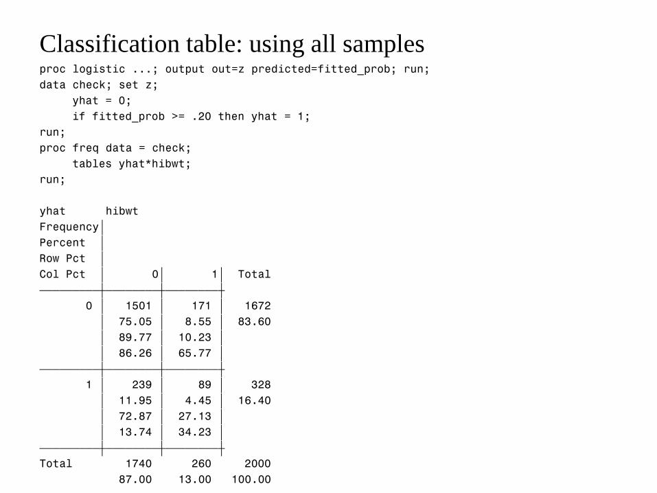
proc logistic ...; output out=z predicted=fitted_prob; run;

data check; set z;

yhat = 0;

if fitted_prob >= .20 then yhat = 1;

run;

proc freq data = check;

tables yhat*hibwt;

run;

yhat hibwt

Frequency‚

Percent ‚

Row Pct ‚



0 ‚ 1501 ‚ 171 ‚ 1672

‚ 75.05 ‚ 8.55 ‚ 83.60

‚ 89.77 ‚ 10.23 ‚

‚ 86.26 ‚ 65.77 ‚


1 ‚ 239 ‚ 89 ‚ 328

‚ 11.95 ‚ 4.45 ‚ 16.40

‚ 72.87 ‚ 27.13 ‚

‚ 13.74 ‚ 34.23 ‚


Total 1740 260 2000

87.00 13.00 100.00

Classification table: using all samples

Classification Table

True Negative False Negative

False Positive True Positive

0

0

0

ˆ1,ˆ for some cutoff

ˆ0,

i

i

ify

if

• Prediction:

• Classification Table:

Sensitivity = TP/(TP+FN); Specificity = TN/(TN+FP).

• Receiver Operating Characteristic (ROC) curve: plot of sensitivity against

1-specificity (i.e., false positive), for possible cutoff π0.

Observed

Pre

dic

tion

0 1

1

0

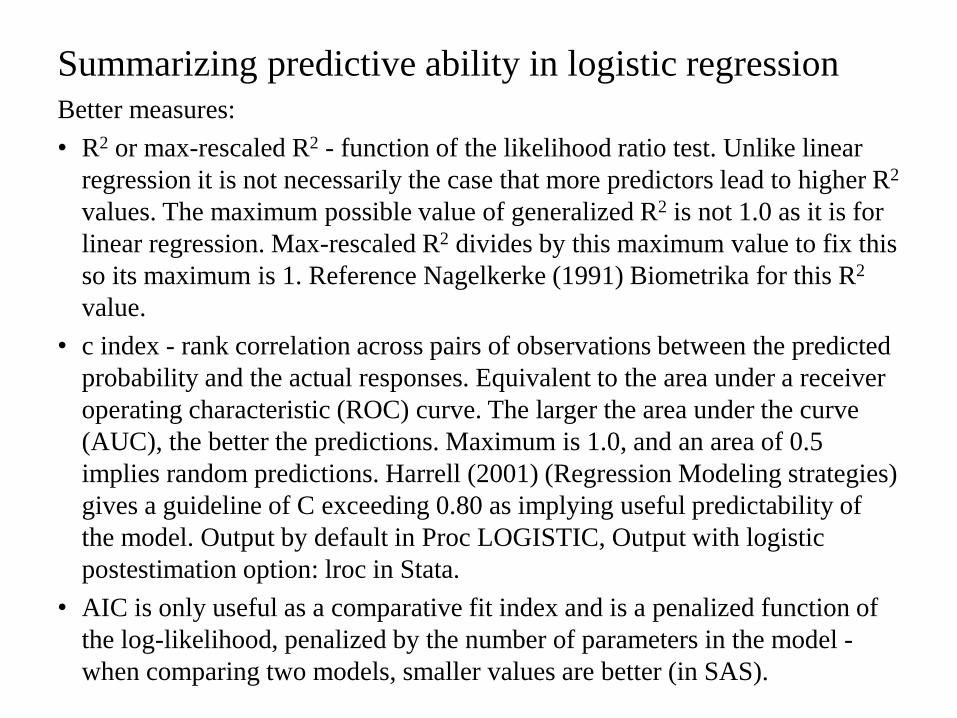
Better measures:

• R2 or max-rescaled R2 - function of the likelihood ratio test. Unlike linear

regression it is not necessarily the case that more predictors lead to higher R2

values. The maximum possible value of generalized R2 is not 1.0 as it is for

linear regression. Max-rescaled R2 divides by this maximum value to fix this

so its maximum is 1. Reference Nagelkerke (1991) Biometrika for this R2

value.

• c index - rank correlation across pairs of observations between the predicted

probability and the actual responses. Equivalent to the area under a receiver

operating characteristic (ROC) curve. The larger the area under the curve

(AUC), the better the predictions. Maximum is 1.0, and an area of 0.5

implies random predictions. Harrell (2001) (Regression Modeling strategies)

gives a guideline of C exceeding 0.80 as implying useful predictability of

the model. Output by default in Proc LOGISTIC, Output with logistic

postestimation option: lroc in Stata.

• AIC is only useful as a comparative fit index and is a penalized function of

the log-likelihood, penalized by the number of parameters in the model -

when comparing two models, smaller values are better (in SAS).

Summarizing predictive ability in logistic regression

Stata: . lroc

area under ROC curve = 0.7031

SAS: Percent Concordant 69.9 Somers' D 0.406

Percent Discordant 29.3 Gamma 0.410

Percent Tied 0.9 Tau-a 0.092

Pairs 452400 c 0.703 <-- area under ROC curve

An annotated explanation of the above values under “Association of Predicted Probabilities” can

be found at https://www.ats.ucla.edu/stat/sas/output/SAS_logit_output.htm

Receiver Operating Characteristic (ROC) curve

0.0

00.2

50.5

00.7

51.0

0

Sen

sitiv

ity

0.00 0.25 0.50 0.75 1.001 - Specificity

Area under ROC curve = 0.7031

1. If this curve was simply a diagonal straight line then the AUC would be

.50 meaning the sensitivity and specificity were never larger than simply

one minus the other, meaning the prediction was no better than a simple

coin flip at fixed probabilities.

2. On the other hand, as the curve bends closer and closer to the upper left

hand corner, the AUC goes to 1 indicating perfect prediction (100%

sensitivity and 100% specificity).

More on ROC curve

Cochran-Armitage Trend Test: test for LINEAR trend in categorical predictor

for 0-1 outcome data. For simple unadjusted relationship, test is performed on

2 by K table where K is the number of categories and Ha is that π1 ≤ π2 ≤ . . . ≤

πK with at least one strict inequality (or visa versa ≥). In linear probability

model:

𝜋𝑗 = 𝛼 + 𝛽𝑠𝑗 , 𝑗 = 1, … , 𝐾

This is to test for H0: β=0.

The test is the same as treating categories as a continuous score with equal

spaced increments in a simple logistic regression and using the overall Score

test.

Can get this test in SAS Proc Freq using the /trend option or of course you can

get it using logistic regression (but it won’t be called the ”Cochran-Armitage

Trend Test” in the output).

Linear trends in 0-1 outcomes for categorical predictors

proc freq;

tables c_baseline_bmi*hibwt / trend;

run;

Statistics for Table of c_baseline_bmi by hibwt

Cochran-Armitage Trend Test

ƒƒƒƒƒƒƒƒƒƒƒƒƒƒƒƒƒƒƒƒƒƒƒƒƒƒƒ

Statistic (Z) -6.5035

One-sided Pr < Z <.0001

Two-sided Pr > |Z| <.0001

===============================================================

proc logistic data = birthwgt2 descending;

model hibwt = c_baseline_bmi;

run;




Score 42.2960 1 <.0001 <--(-6.5035)^2 = 42.296

Wald 40.9012 1 <.0001

*. In Stata, install –ptrend- command for trend test . ptrendi 3 159 1 \ 95 850 2 \ 54 257 3 \ 108 474 4

Chi2(1) for trend = 42.296, pr>chi2 = 0.0000

Linear trends in 0-1 outcomes for categorical predictors

The Pearson statistic is:

The Residual Deviance statistic is:

2[logL(saturated model) − logL(the current model)]

These do not work properly for logistic regression except when there are only

a few categorical predictors leading to aggregated data with large cell counts.

Their validity relies on the assumption of large numbers of observations in

binomial cells and both tests show unsatisfactory behaviour with sparse data.

In fact with continuous predictors they can be shown to be completely

meaningless (since continuous predictors lead to only one observation within

every cell - sparse data). These statistics are NOT output by SAS when using

Proc Logistic or Proc Genmod when the binomial distribution is specified

(although they are output when Poisson distribution is specified). On the other

hand, these statistics are output by Stata in the glm output even for binomial

distribution.

Goodness of Fit

A solution to the problems associated with the Pearson and Residual Deviance

for binomial regression comes from the Hosmer Lemeshow test which groups

the data before forming a chi-square type statistic.

The Hosmer-Lemeshow Statistic is a measure of lack of fit in a logistic

regression model. Hosmer and Lemeshow recommend partitioning the

observations into 10 equal sized groups according to their predicted

probabilities. The test then computes a chi-square statistic from observed and

expected frequencies in each of the 10 quantiles. The null is that the observed

frequencies equal the expected frequencies, hence if we do NOT reject the null

then we are saying the model is well-fitting, i.e. there is no significant

difference between observed and model-predicted values.

In SAS: Get this statistics use the /lackfit option

In STATA: use the postestimation option: lfit, group(10) table

Goodness of Fit - Hosmer Lemeshow test

proc logistic data = birthwgt2 descending;

class c_baseline_bmi (ref = "2") /param = ref;

model hibwt = totalweightgain c_baseline_bmi/rsq ctable pprob = (.13) lackfit;

output out=z predicted =fitted_prob;

run;

Partition for the Hosmer and Lemeshow Test

hibwt = 1 hibwt = 0

Group Total Observed Expected Observed Expected

1 209 5 4.96 204 204.04

2 199 9 11.75 190 187.25

3 200 7 15.24 193 184.76

4 199 25 17.76 174 181.24

5 188 17 19.42 171 168.58

6 208 29 24.98 179 183.02

7 205 25 29.12 180 175.88

8 205 46 34.74 159 170.26

9 199 45 42.28 154 156.72

10 188 52 59.75 136 128.25

Hosmer and Lemeshow Goodness-of-Fit Test

Chi-Square DF Pr > ChiSq

16.5844 8 0.0347

Goodness of Fit: SAS output

. estat gof, group(10) table

Logistic model for hibwt, goodness-of-fit test

(Table collapsed on quantiles of estimated probabilities)

+--------------------------------------------------------+

| Group | Prob | Obs_1 | Exp_1 | Obs_0 | Exp_0 | Total |

|-------+--------+-------+-------+-------+-------+-------|

| 1 | 0.0473 | 5 | 5.0 | 204 | 204.0 | 209 |

| 2 | 0.0668 | 8 | 11.5 | 187 | 183.5 | 195 |

| 3 | 0.0819 | 8 | 15.0 | 190 | 183.0 | 198 |

| 4 | 0.0949 | 25 | 17.9 | 176 | 183.1 | 201 |

| 5 | 0.1122 | 19 | 22.7 | 199 | 195.3 | 218 |

|-------+--------+-------+-------+-------+-------+-------|

| 6 | 0.1294 | 27 | 22.1 | 155 | 159.9 | 182 |

| 7 | 0.1541 | 25 | 29.1 | 180 | 175.9 | 205 |

| 8 | 0.1849 | 46 | 34.7 | 159 | 170.3 | 205 |

| 9 | 0.2389 | 44 | 40.1 | 146 | 149.9 | 190 |

| 10 | 0.6046 | 53 | 61.9 | 144 | 135.1 | 197 |

+--------------------------------------------------------+

number of observations = 2000

number of groups = 10

Hosmer-Lemeshow chi2(8) = 17.15

Prob > chi2 = 0.0286

Note: SAS and Stata outputs are different because they handle the ties

differently.

Goodness of Fit: Stata output

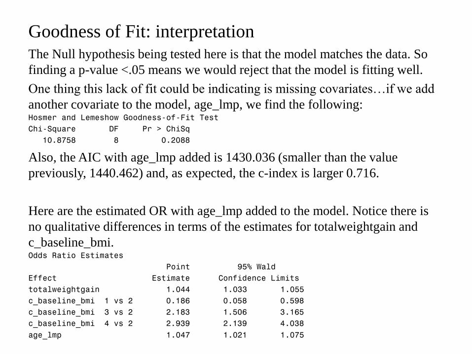
The Null hypothesis being tested here is that the model matches the data. So

finding a p-value <.05 means we would reject that the model is fitting well.

One thing this lack of fit could be indicating is missing covariates…if we add

another covariate to the model, age_lmp, we find the following: Hosmer and Lemeshow Goodness-of-Fit Test

Chi-Square DF Pr > ChiSq

10.8758 8 0.2088

Also, the AIC with age_lmp added is 1430.036 (smaller than the value

previously, 1440.462) and, as expected, the c-index is larger 0.716.

Here are the estimated OR with age_lmp added to the model. Notice there is

no qualitative differences in terms of the estimates for totalweightgain and

c_baseline_bmi. Odds Ratio Estimates

Point 95% Wald

Effect Estimate Confidence Limits

totalweightgain 1.044 1.033 1.055

c_baseline_bmi 1 vs 2 0.186 0.058 0.598

c_baseline_bmi 3 vs 2 2.183 1.506 3.165

c_baseline_bmi 4 vs 2 2.939 2.139 4.038

age_lmp 1.047 1.021 1.075

Goodness of Fit: interpretation

NOTE: This test is known to be highly dependent on the actual groupings (the

number of groups) and cutoff value used when conducting the test. It also

tends to detect small differences when the sample size is large. VGSM

reccommend using it cautiously.

NOTE: This test does not have anything to do with whether regression

coefficients are significant or whether there is high predictability (e.g. high c-

statistic) in the model.

From: “A comparison of goodness-of-fit tests for the logistic regression

model” by DS Hosmer, T Hosmer, SL Cessie, and S Lemeshow Statistics in

Med., VOL. 16, 965-980 (1997)

In the context of logistic regression the overall goodness of fit is assessing all

of the following (not any one specifically)

• The logit transformation is the correct function linking covariates with the

conditional mean Xβ

• The linear predictor is correct, i.e. we do not need to include additional

variables, transformation of variables, or interactions of variables

• The variance is Bernoulli, i.e. var(Y |X) = π(X)(1 − π(X))

Goodness of Fit - Hosmer Lemeshow test

SAS will not produce odds ratios when you include an interaction in a logistic

regression. Stata will still produce odds ratios which are simply the

exponential of the estimated coefficients.

-- We cannot interpret the coefficient of one predictor as a log odds ratio

without specifying value of the other predictor.

-- Since the predictor X is involved in both main and interaction terms,

OR(Y|X) = odds(Y|X+1)/odds(Y|X) needs to be computed using both the

estimated coefficients for main and interaction terms.

Complete seminar about how to do this: Statistical Computing Seminars

Visualizing Main Effects and Interactions for Binary Logit Models in Stata

http://www.ats.ucla.edu/stat/stata/seminars/stata_vibl/default.htm

Interactions in models with 0-1 outcomes

proc logistic data = wcgs descending;

class bage_50 (ref = "0") arcus (ref = "0") /param = ref;

model chd69 = bage_50 arcus bage_50*arcus;

contrast 'OR(arcus) in older group' arcus 1 bage_50*arcus 1 1 / estimate=exp;

run;

Standard Wald

Parameter DF Estimate Error Chi-Square Pr > ChiSq

Intercept 1 -2.8828 0.1089 700.4573 <.0001

arcus 1 1 0.6480 0.1789 13.1236 0.0003

bage_50 1 1 0.8933 0.1721 26.9328 <.0001

bage_50*arcus 1 1 1 -0.5920 0.2722 4.7299 0.0296

Contrast Type Row Estimate Error Alpha Confidence Limits

OR(arcus) in older group EXP 1 1.0575 0.2170 0.05 0.7073 1.5811

Interpretation of the interaction term is similar to that in linear regression

model. Instead of difference in the slope, it is now the difference in log(Odds

Ratio). For example,

Interactions: age group * presence of arcus senilis

Interactions: component odds ratios

Interactions: categorical and continuous predictors

Documents

Binary Outcomes Logistic Regression (Chapter 6)wguan/class/PUBH7402/notes/le… · · 2015-03-10Binary Outcomes – Logistic Regression (Chapter 6) • 2 by 2 tables • Odds ratio,