Bio-Driven Cell Region Detection in HumanEmbryonic Stem Cell Assay

Benjamin X. Guan, Bir Bhanu, Prue Talbot, andSabrina Lin

Abstract—This paper proposes a bio-driven algorithm that detects cell regions

automatically in the human embryonic stem cell (hESC) images obtained using a

phase contrast microscope. The algorithm uses both statistical intensity

distributions of foreground/hESCs and background/substrate as well as cell

property for cell region detection. The intensity distributions of foreground/hESCs

and background/substrate are modeled as a mixture of two Gaussians. The cell

property is translated into local spatial information. The algorithm is optimized by

parameters of the modeled distributions and cell regions evolve with the local cell

property. The paper validates the method with various videos acquired using

different microscope objectives. In comparison with the state-of-the-art methods,

the proposed method is able to detect the entire cell region instead of

fragmented cell regions. It also yields high marks on measures such as

Jacard similarity, Dice coefficient, sensitivity and specificity. Automated

detection by the proposed method has the potential to enable fast quantifiable

analysis of hESCs using large data sets which are needed to understand

dynamic cell behaviors.

Index Terms—Automated detection, bioinformatics, bio-driven, human embryonic

stem cell (hESC)

Ç

1 INTRODUCTION

HUMAN embryonic stem cells (hESCs) are pluripotent cellsderived from the inner cell mass of blastocysts, and in culture,they closely resemble epiblast cells of gastrulating embryos [1],[2]. Due to fact that hESCs have the ability to self renew indefi-nitely and to differentiate into all three germ layers (ectoderm,endoderm, and mesoderm), they are widely used in researchdesigned to tap their potential for treating degenerative dis-eases. In addition, hESCs provide one of the best models cur-rently available for assessing the toxicity of environmentalchemicals on prenatal development [3], [4].

Application of video bioinformatics tools to hESC problemscan greatly accelerate research in both regenerative and preven-tive medicine. As an example, a video analysis method for quan-tifying the rate of hESC colony growth was used to evaluate thetoxicity of cigarette smoke from conventional and harm reduc-tion cigarettes [5], [6]. The hESCs were imaged over time usinga high content Nikon BioStation IM incubation unit equippedwith a phase contrast microscope. Time-lapse videos were eval-uated quantitatively for colony growth during treatment withcigarette smoke. Analysis showed that side-stream smoke from“harm reduction” brands of cigarettes was as harmful as oreven more harmful than side-stream smoke from a conventionalbrand [5].

Cell region detection using the BioStation’s cell analysis soft-ware is done either manually or in a semi-automatic manner [6].The fastest rate at which BioStation IM can collect data is oneframe per two seconds. In the current study, a new video bioin-formatics tool is developed to further enhance the analysis ofhESC video data. With this new tool, cell regions are detected

using a bio-driven algorithm that uses a mixture of two Gaus-sians and exploits properties of hESCs. Once cell regions aredetected, quantitative data can be utilized to determine the rateof hESC growth and numerous other parameters related to itsuch as its blebbing and attachment behavior. Therefore, highsensitivity and specificity on cell region detection are significant.Most importantly, the proposed method requires only 1.2 sec-onds of processing time per frame on a laptop with a Intel(R)Core 2 Duo CPU processor that runs at 2.53 GHz, it can performcell analysis concurrently with the BioStation which is collectinglive video data. The establishment of an automated and accuratecell detection tool is valuable and necessary for studyingdynamic processes in hESCs.

2 RELATED WORK AND CONTRIBUTIONS

K-means algorithm and mixture of Gaussians using an Expecta-tion-Maximization (EM) algorithm are widely used techniquesfor image segmentation. K-means segmentation algorithm byTatiraju and Mehta [7] considered each pixel intensity value asan individual observation. It partitions these observations into Kclusters in which each observation belongs to the cluster with thenearest mean intensity value [8], [9]. However, the method doesnot consider the intensity distribution of its clusters. In contrast,the mixture of Gaussians segmentation method using the EM(MGEM) algorithm proposed by Farnoosh and Zarpak [10]depends heavily on intensity distribution models to group theimage data. The MGEM method assumes the image’s intensitydistribution can be represented by multiple Gaussians [7], [11],[12]. However, it does not take into account the neighborhoodinformation. As a result, segmented regions obtained by theabove algorithms lack connectivity with the pixels within theirneighborhoods. This lack of connectivity of a pixel with its neigh-borhood pixels is due to the following two characteristics ofhESC images (see Fig. 1): i) an incomplete halo surrounds the cellbody; ii) cell body intensity values are similar to the substrateintensity values [13].

State of the art CL-Quant software [14] for bioinformatic imageanalysis requires users to make a recipe for the experimental dataand the recipe is created with the data itself. It is semi-automatic,and its performance is heavily depended on the recipe maker.Our proposed method is intended to solve the connectivity prob-lems by using cell property as well as the cell and substrate inten-sity distributions. The cell property manifests itself in spatialinformation where cell regions have a high intensity variation.This variation in cell region is due to the organelles inside the cell.We evolve the cell regions based on spatial information until theoptimal intensity distributions of background (substrate) andforeground (hESCs) regions are obtained. The optimization isdone on the original image and the spatial evolution is based onthe spatial characteristic. The proposed method is bio-driven, fastand automated.

3 TECHNICAL APPROACH

In this section, we first explain the optimization metric modeledas a mixture of two Gausians, and its convergence. We thenelaborate on hESC property as spatial information. The handlingof noise and over-segmentation are also discussed in thissection. For the convenience of a reader, a summary of the sym-bols used in paper is provided in Table 1.

3.1 Optimization Metric

The hESCs were cultured in vitro using methods described in detailpreviously [15]. The hESCs are grown in culture dishes coated witha layer of substrate (Matrigel). The substrate becomes the back-ground after the hESCs are placed on its surface. Therefore, we

� B.X. Guan and B. Bhanu are with the Center for Research in Intelligent Systems andthe Department of Electrical Engineering, University of California-Riverside, River-side, CA 92521. E-mail: xguan001@ucr.edu, bhanu@cris.ucr.edu.

� P. Talbot and S. Lin are with the Stem Cell Center, University of California-Riverside, Riverside, CA 92521. E-mail: {talbot, sabrina.lin}@ucr.edu.

Manuscript received 31 Aug. 2013; revised 10 Jan. 2014; accepted 31 Jan. 2014.Date of publication 18 Feb. 2014; date of current version 5 June 2014.For information on obtaining reprints of this article, please send e-mail to:reprints@ieee.org, and reference the Digital Object Identifier below.Digital Object Identifier no. 10.1109/TCBB.2014.2306836

604 IEEE/ACM TRANSACTIONS ON COMPUTATIONAL BIOLOGY AND BIOINFORMATICS, VOL. 11, NO. 3, MAY/JUNE 2014

1545-5963� 2014 IEEE. Personal use is permitted, but republication/redistribution requires IEEE permission.See http://www.ieee.org/publications_standards/publications/rights/index.html for more information.

model a hESC image with two regions of interest: foreground andbackground. Fig. 2 shows that the intensity distributions of theseregions are similar to a mixture of two Gaussians with differentmeans and variances. Consequently, we model the intensity distri-bution of foreground (cell region with a mean mf and variance s2

f )

and background (substrate region with a mean mb and variance s2b )

as the mixture of two Gaussians. Fig. 3 shows our model.With this model, we then want to maximize the absolute differ-

ence of two mean-to-variance ratios (MVRs); the absolute differ-ence of the foreground MVR and background MVR. The MVRs ofthe foreground and background data sets are calculated by the fol-lowing equations [16]:

MVRf ¼ mf

s2f

; (1)

MVRb ¼ mb

s2b

; (2)

whereMVRf andMVRb are the MVRs for the foreground and back-ground data sets, respectively.

The optimization metric M is formulated as

M ¼ MVRf �MVRb

�� ��: (3)

Substituting (1) and (2) into (3), we get the following:

M ¼ mf

s2f

� mb

s2b

����������: (4)

Equation (4) shows the metric that is used to determine howmuch the cell region data are different from the substrate regiondata. Since the algorithm is spatially evolving the foregroundregion from the initial high intensity variation region by a mean

filter at each iteration, the foreground mean and variance are

approaching to the background mean and variance. The limit of

M is 0 asmf

s2f

approaches to mb

s2b

. Therefore, our problem becomes

finding Mopt which is the optimal value for metric M, and the cor-

responding equation is described below:

Mopt ¼ maxmf ;s

2f;mb;s

2b

M�mf ; s

2f ;mb; s

2b

�: (5)

Mopt finds the parameters that maximize the difference betweenforeground and background data.

3.2 Convergence of the Metric

The convergence of metric M can be proven from experiments.Fig. 4 shows the metric M at each iteration for all objectives with/without filtering.

3.3 Spatial Information and Intensity Distribution

The hESC region, F, is a high intensity variation region while thesubstrate region, B, is a low intensity variation region. As a result,we are able to exploit the gradients of the image to segment out thecell region from the substrate region. The following equationsshow how we exploit the gradients of the image:

Fig. 1. (a)-(b). Cells with incomplete halo and similar substrate intensity values.

TABLE 1Definition of the Symbols Used in This Paper

Fig. 2. Foreground and background intensity distributions for each data set.

IEEE/ACM TRANSACTIONS ON COMPUTATIONAL BIOLOGY AND BIOINFORMATICS, VOL. 11, NO. 3, MAY/JUNE 2014 605

I ¼ F [B; (6)

G ¼ dI

dx

� �2

þ dI

dy

� �2

; (7)

IG ¼ logeð�1þ eÞ �G

maxðGÞ þ 1

� �� 255; (8)

where G is the squared gradient magnitude of image, I. dIdx and

dIdy

are gradients of image, I, in the x and y directions, respectively.IG is the spatial information produced by (8), which furtheremphasizes the difference between cell and substrate regions.Equation (8) normalizes G. The inner component of naturallog transformation, ð�1þ eÞ �G=maxðGÞð Þ þ 1, ensures that thetransformation result will be within the range from 0 to 1. WhenG is 0, then logeð1Þ is equal to 0. When G is equal to the max ofG, then logeðeÞ is equal to 1 and IG is equal to 255. The naturallog function transforms a narrow range of small input valuesinto a wider range of output values. Equation (8) is essentially agamma correction technique [17]. It creates a large intensity sep-aration between the foreground and background. Therefore, thenatural log transformation enhances the image’s intensity distri-bution to become a more visible bimodal distribution.

The proposed algorithm also uses a mean filter on IG at eachiteration to evolve the cell regions. It is able to group the cell regionpixels together based on local information; the size of the mean fil-ter dictates how fast the cell region is evolved. The method updatesIG and evolves the cell region untilM is maximized.

Equation (4) is calculated based on the mean and variance ofthe intensity distributions of the cell and substrate data. Thecell region, F, and substrate region, B, are updated by thresh-olding IG with OTSU’s method at each iteration [17]. The inten-sity distribution’s mean and variance of the cell region andsubstrate region data are also updated at each iteration by thefollowing equations:

mf ¼P

f2F f

Nf; (9)

mb ¼P

b2B b

Nb; (10)

s2f ¼

Pf2F ðf � mf Þ2

Nf; (11)

s2b ¼

Pb2B b� mbð Þ2

Nb; (12)

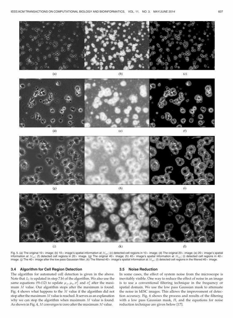
where Nf and Nb are the total numbers of foreground and back-ground pixels in the image, f and b are the intensity values inthe corresponding foreground and background. Fig. 5 shows theintermediate and final results of the proposed method on vari-ous images. Figs. 5b, 5e, 5h and 5k show the spatial informationwhen Mopt is reached for their respective data.

Fig. 3. Intensity distribution model of foreground and background. Fig. 4. Metric values at each iteration for images under different objectives.

606 IEEE/ACM TRANSACTIONS ON COMPUTATIONAL BIOLOGY AND BIOINFORMATICS, VOL. 11, NO. 3, MAY/JUNE 2014

3.4 Algorithm for Cell Region Detection

The algorithm for automated cell detection is given in the above.Note that IG is updated in step 7.b) of the algorithm. We also use thesame equations (9)-(12) to update mf ;mb; s

2f and s2

b after the maxi-mum M value. Our algorithm stops after the maximum is found.Fig. 4 shows what happens to the M value if the algorithm did notstop after themaximumM value is reached. It serves as an explanationwhy we can stop the algorithm when maximum M value is found.As shown in Fig. 4,M converges to zero after themaximumM value.

3.5 Noise Reduction

In some cases, the effect of system noise from the microscope isinevitably visible. One way to reduce the effect of noise in an imageis to use a conventional filtering technique in the frequency orspatial domain. We use the low pass Gaussian mask to attenuatethe noise in hESC images. This allows the improvement of detec-tion accuracy. Fig. 6 shows the process and results of the filteringwith a low pass Gaussian mask, H, and the equations for noisereduction technique are given below [17].

Fig. 5. (a) The original 10� image; (b) 10� image’s spatial information atMopt; (c) detected cell regions in 10� image; (d) The original 20� image; (e) 20� image’s spatialinformation at Mopt; (f) detected cell regions in 20� image. (g) The original 40� image; (h) 40� image’s spatial information at Mopt; (i) detected cell regions in 40�image. (j) The 40� image after the low pass Gaussian filter; (k) The filtered 40� image’s spatial information atMopt; (l) detected cell regions in the filtered 40� image.

IEEE/ACM TRANSACTIONS ON COMPUTATIONAL BIOLOGY AND BIOINFORMATICS, VOL. 11, NO. 3, MAY/JUNE 2014 607

hgaus r; cð Þ ¼ e�ðr�rcÞ2þðc�ccÞ2

2s2gaus ; (13)

H r; cð Þ ¼ hgaus r; cð ÞPr

Pc hgaus r; cð Þ; (14)

IF ¼ F�1 F If g � F Hf gf g: (15)

IF and H have the same dimensionality as image, I, where it hasR rows and C columns. r 2 1; : : ; Rf g and c 2 1; : : ; Cf g: hgausðr; cÞ isa low pass Gaussian mask value at location r; cð Þ and sgaus is thestandard deviation of the Gaussian mask. ðrc; ccÞ has the valueðR=2; C=2Þ which is the center location of the mask. F �f g is a 2DFourier transform operation, and F�1 �f g is the inverse 2D Fouriertransform operation.

3.6 Over-Segmentation Reduction

Since the mean filter is used to evolve the foreground region, over-segmentation is inevitable. Therefore, we use a morphological ero-sion technique to reduce the error caused by over-segmentationafter the foreground and background regions have been detected[17]. In this paper, we use a common disk structuring element forthe morphological erosion technique, and the erosion parameter isits radius. The erosion parameter is identified from a receiver oper-ating characteristic (ROC) curve where a minimum of 90 percenttrue positive rate and a false positive rate (FPR) lower than 10 per-cent are achieved for each data set with/without filtering [18].The first image of each data set is used to determine the erosionparameter and it is used for all the remaining images in a dataset. The higher value of erosion parameter can lead to under-segmentation. However, if the erosion parameter is close tozero, over-segmentation can still exist. Since 40� image does notmeet the above criteria, no erosion parameter is selected for it.Fig. 7 shows the ROC and the optimal points where the erosionparameters are picked.

The detected foreground and background regions have associ-ated masks (binary images). The morphological erosion operationis applied to the foreground region with the erosion parameterfound from Fig. 7. Since the foreground and background regionsare complement of each other, the updated background regioncan be derived directly from the updated foreground region.

4 EXPERIMENTAL RESULTS

4.1 Data

All time lapse videos were obtained with a BioStation IM [19].The frames in the video are phase contrast images with 600 � 800resolution. The videos were acquired using three different objec-tives: 10�, 20� and 40� and each objective has a set of 40 images,with a total of 120 images. Each video frame is taken roughly2 minutes apart for the purpose of data variation from frame toframe. The ground-truth is generated manually by the expertbiologists.

Note that for all the video data used in this paper, the hESCculture conditions are considered to be excellent. All videosused are of small colonies or single hESC, and the cells lookexcellent for unattached hESCs and colonies. Most hESC culturetoday is not done on mouse embryonic fibroblasts (MEFs). Wehave not cultured hESC on feeders since 2008. We use mTeSRmedium [20]. This modern culture media does not require theuse of MEFs, so they are seldom used. With an exception formaintenance, MEFs are not used in experiments. Since it ishighly unlikely that we will analyze hESC cultured on MEFs,we have not tested our algorithms on data sets with hESC cul-tured on MEFs. Moreover, the images in this manuscript havevery few dead cells and debris. In fact, they are remarkablyclean considering the cells have been stripped and replated.

4.2 Parameters

Each video collected with different objectives has a differentdefault size of neighborhood for spatial grouping. The default sizesare determined by observing the ROC plots with various windowsizes for each objective. Based on the experimental analysis in [13],we concluded that the optimal neighborhood sizes for 10�, 20�and 40� are 5� 5, 7� 7 and 11 � 11, respectively. The selection cri-teria for the neighborhood sizes are based on finding a window forwhich its ROC plot yields a high true positive rate while keepingthe low false positive rate. A low pass Gaussian mask with a stan-dard deviation equal to 80 pixels is used to get rid of the noise thatoccurs during the video acquisition process. For the erosion param-eter which is discussed in Section 3.6, we use a disk with radius 2,5, 4, 8, 0, and 1 for 10�, filtered 10, 20, filtered 20�, 40� and filtered40� data sets, respectively.

4.3 Performance Measures

The true positive, TP, is the overlapped region between thedetected cell region and the cell region ground-truth. Truenegative, TN, is the overlapped region between the detected

Fig. 6. (a) The original noisy 40� image; (b) noisy 40� image after 2D Fouriertransformation; (c) low pass Gaussian mask with standard deviation equal to 80;(d) resulting image after noise filtering.

Fig. 7. ROC plots for images under different objectives with varying erosionparameter.

608 IEEE/ACM TRANSACTIONS ON COMPUTATIONAL BIOLOGY AND BIOINFORMATICS, VOL. 11, NO. 3, MAY/JUNE 2014

background region and the background ground-truth. The falsepositive, FP, is the detected background that is falsely identified aspart of the cell region. The false negative, FN, is the detected cellregion that is falsely identified as part of the background.

The true positive rate or sensitivity, TPR or SEN, measures theproportion of actual positives which are correctly identified:

TPR ¼ TP

TP þ FNð Þ: (16)

The false positive rate, measures the proportion of false posi-tives which are incorrectly identified:

FPR ¼ FP

FP þ TNð Þ: (17)

The specificity, SPC, is the true negative rate which is a com-plement of false positive rate:

SPC ¼ TN

FP þ TNð Þ: (18)

The Jaccard similarity, JAC, is a measure of similarity betweenexperimental results and the ground-truth:

JAC ¼ TP

TP þ FP þ FNð Þ: (19)

The Dice coefficient, DIC, measures the agreement betweenexperimental results and ground-truth:

DIC ¼ 2TP

2TP þ FP þ FNð Þ: (20)

The average detection error is an average of type I (1-SPC) andtype II (1-SEN). ANOVA test [21] is also used for comparison ofdetected foreground and background intensity distributions withthe corresponding ground-truth intensity distributions.

4.4 Methods Compared

We compared the proposed method with k-means, Mixture ofGaussians, and CL-Quant software with various recipes [7], [10],[14]. In addition, we evaluated the data sets with Otsu’s algorithm[17]. However, it was not able to detect the entire cell region due tofact that the intensity values of the cell body are similar to the sub-strate intensity values. As shown in Fig. 8, the result was not use-ful. Therefore, Otsu’s algorithm is not compared in this paper.

Note that we do not compare this work with our work in refer-ence [5] which is concerned with the growth of attached hESCs.This is quite different from the current study. In this study, theimages are comprised of single cells and small colonies. The smallcolonies are cell colonies that contain more than two cells. Fromimage processing point of view, the detection of large cell coloniesis much easier than detection of all individual cell regions in thelow cell confluence images. We are not focused with the detectionof large cell colonies in this paper. Here we are concerned withusing basic image properties of hESCs to extract individual cellregions. The detection algorithm exploits the high intensityvariation within the cell body due to the presence of organelles.Most importantly, CLQuant is able to detect the large cell coloniesafter training as discussed [5]. However, the data sets used inthis paper are much more challenging to CLQuant even after exten-sive training.

TABLE 2Comparisons of 10� Data Set (� Denotes Filtered Data)

Fig. 8. (a) The original 10� image; (b) binary result of (a) with Otsu’s; (c) the origi-nal 20� image; (d) binary result of (c) with Otsu’s; (e) the original 40� image; (f)binary result of (e) with Otsu’s.

TABLE 3Comparisions of 20� Data Set (� Denotes Filtered Data)

IEEE/ACM TRANSACTIONS ON COMPUTATIONAL BIOLOGY AND BIOINFORMATICS, VOL. 11, NO. 3, MAY/JUNE 2014 609

4.5 Results and Discussion

The proposed method was tested with three videos (each with40 frames) that were acquired with 10�, 20� and 40� objectives.The proposed method achieved above 90 percent in sensitivityand specificity on 10� with/without filtering, 20� with/withoutfiltering and 40� with filtering data sets. Since pre-filtering getsrid of high frequency noise, it improves the performance of theproposed algorithm on noisy data. The 10 and 20� data sets arenot corrupted with high frequency noise. Therefore, pre-filtering

on those data sets would not affect the algorithm’s performanceon JAC, DIC, SEN and SPC measures as shown in Tables 2and 3. However, the 40� data set is corrupted with high fre-quency noise. The pre-filtering improves the yield on its SENmeasure significantly as shown in Table 4.

In this paper, we compared the proposed method with K-means, mixture of Gaussians segmentation method and CL-Quant software under different recipes. Tables 2, 3, and 4 showthe results of the K-means, MGEM segmentation, CL-Quant soft-ware, and the proposed method on all experimental data. Theproposed method outperforms the other methods in JAC andDIC measures. Moreover, the proposed method yields above

TABLE 4Comparisons of 40� Data Set (� Denotes Filtered Data)

TABLE 5Average Detection Errors of Foreground and Background

Fig. 9. ANOVA test of foreground and background distributions for all data sets. SS ¼ sum of squares, df ¼ degree of freedom, MS ¼ mean square, F ¼ F-statistic, [] ¼not applicable.

610 IEEE/ACM TRANSACTIONS ON COMPUTATIONAL BIOLOGY AND BIOINFORMATICS, VOL. 11, NO. 3, MAY/JUNE 2014

90 percent in both SEN and SPC measures. K-means clusters theimage data based only on the nearest mean while the MGEMmethod groups the data solely on the modeled intensity distri-bution. Consequently, neither method was able to detect theentire cell regions. Instead, they have detected fragments ofthe actual cell regions. Their performance is further degraded bythe presence of noise. The CL-Quant software’s performancedepends heavily on the recipe maker. The recipes for the datasets used in this paper are created by a fourth year biology PhDstudent. More importantly, the proposed method’s performanceis good on the image data with or without filtering.

In terms of performance, the proposed method yields lowerthan 10 percent average detection error of foreground and back-ground on 10 and 20� with/without filtering, and 40� with filter-ing data sets as shown in Table 5. MGEM has a minimum of 14.17percent and a maximum of 20.14 percent average detection error[10]. K-means algorithm yields above 25 percent average detectionerror on all data sets [7]. CL-Quant gives a minimum of 12.05 per-cent and a maximum of 21.84 percent average detection error [14].In terms of convergence, the proposed method converges in seveniterations on the average, and each iteration requires 0.17 second. Itreaches the global optimum since the mean filter is used for group-ing similar regions in the algorithm.

5 CONCLUSIONS

The proposed method incorporated the concept of local property ofa hESC as well as cell and substrate intensity distributions for cellregion detection in phase contrast images. It uses the spatial infor-mation to improve the connectivity of local pixels to their corre-sponding regions. More importantly, it enables fast convergence tothe maximum absolute difference of foreground and backgroundmean-to-variance ratios. The proposed method is able to split theimage data into two Gaussian distributions; intensity distributionof the foreground and background data. Table 5 shows that theproposed method yields a lower average detection error than theK-means, MGEM and CL-Quant methods [7], [10], [14]. Fig. 9shows an ANOVA test for all experimental data sets. It shows lowerror in comparison between the intensity distributions of the pro-posed method and the ground-truth intensity distributions. In thecase of noisy images, the pre-filtering of the image data can greatlyimprove the performance of the algorithm. In term of speed, theproposed method converges in less than 1.2 seconds while K-means and MGEM take about 3.61 and 25.3 seconds respectivelyon a laptop with a Intel(R) Core 2 Duo CPU processor that run at2.53 GHz. The CL-Quant software requires at least six minutes ofuser inputs from the expert biologist for each recipe. Applicationof this automated method to hESC will facilitate the analysis oftheir dynamic behaviors and benefit research in both regenerativeand preventive medicine.

It is to be noted that the proposed method studies single cellsand small colonies after plating before the cells are attached. Differ-entiation would not be a factor unless cells are first attached andthen incubated for at least 24 hours in a medium that supports dif-ferentiation. Our method works on cells that have high intensityvariation on their cell bodies. As long as this image propertystill holds for dead cells, differentiated and undifferentiated/pluripotent hESCs, we can detect them. The proposed cell regiondetection is a start for an automated cell region detection and cellclassification. With the automated cell region detection, we canmove forward our research for an automated classification system.

ACKNOWLEDGMENTS

This research was supported by NSF-IGERT: Video BioinformaticsGrant DGE 0903667 and by Tobacco-Related Disease Research Pro-gram (TRDRP): Grant 20XT-0118 and by a TRDRP Postdoctoral

Fellowship (20FT-0084). The authors would like to thank Jo-HaoWeng for making the CL-Quant software recipes.

REFERENCES

[1] J.A. Thomson et al., “Embryonic Stem Cell Lines Drived from HumanBlastocysts,” Science, vol. 282, no. 5395, pp. 1145-1147, Nov. 1998.

[2] J. Nichols and A. Smith, “The Original and Identity of Embryonic StemCells,” Development, vol. 138, pp. 3-8, Jan. 2011.

[3] M. Stojkovic, M. Lako, T. Strachan, and A. Murdoch, “Derivation, Growthand Applications of Human Embryonic Stem Cells,” Reproduction, vol. 128,pp. 259-267, Sept. 2004.

[4] P. Talbot and S. Lin, “Mouse and Human Embryonic Stem Cells: Can TheyImprove Human Health by Preventing Disease?” Current Topics in Medici-nal Chemistry, vol. 11, no. 13, pp. 1638-1652, 2011.

[5] S. Lin et al., “Comparison of the Toxicity of Smoke from Conventional andHarm Reduction Cigarettes Using Human Embryonic Stem Cells,” ToxicolScience, vol. 118, pp. 202-212, Aug. 2010.

[6] S. Lin et al., “Video Bioinformatics Analysis of Human Embryonic StemCell Colony Growth,” J. Visualized Experiments, vol. 39, pp. 1-5, May 2010.

[7] S. Tatiraju and A. Mehta, “Image Segmentation Using K-Means Clustering,EM and Normalized Cuts,” pp. 1-7, http://www.ics.uci.edu/~dramanan/teaching/ics273a_winter08/projects/avim_report.pdf, UC Irvine, 2008.

[8] K. Alsabti, S. Ranka, and V. Singh, “A Efficient K-Means Clustering Algo-rithm,” Proc. First Workshop High Performance Data Mining, 1998.

[9] T. Kanungo, D.M. Mount, N.S. Netanyahu, C.D. Piatko, R. Silverman, andA.Y. Wu, “An Efficient K-Means Clustering Algorithm: Analysis andImplementation,” IEEE Trans. Pattern Analysis and Machine Intelligence,vol. 24, no. 7, pp. 881-892, July 2002.

[10] R. Farnoosh and B. Zarpak, “Image Segmentation Using Gaussian MixtureModel,” Int’l J. Eng. Science, vol. 19, pp. 29-32, 2008.

[11] L. Xu and M.I. Jordan, “On Convergence Properties of the EM Algorithmfor Gaussian Mixture,” Neural Computation, vol. 8, pp. 129-151, 1996.

[12] S. Gopinath, Q. Wen, N. Thakoor, K. Luby-Phelps, and J.X. Gao, “A Statisti-cal Approach for Intensity Loss Compensation of Confocal MicroscopyImages,” J. Microscopy, vol. 230, pp. 143-159, 2008.

[13] B.X. Guan, B. Bhanu, P. Talbot, and S. Lin, “Automated Human EmbryonicStem Cell Detection,” Proc. IEEE Second Int’l Conf. Healthcare Informatics,Imaging and Systems Biology, pp. 75-82, Sept. 2012.

[14] Nikon. CL-Quant, http://www.nikoninstruments.com/News/US-News/Nikon-Instruments-Introduces-CL-Quant-Automated-Image-Analysis-Software,July 2013.

[15] S. Lin and P. Talbot, “Methods for Culturing Mouse and Human Embry-onic Stem Cells,”Methods Molecular Biology, vol. 690, pp. 31-56, 2011.

[16] J. Bushberg, J. Seibert, E. Leidholdt, and J. Boone, The Essential Physics ofMedical Imaging. second ed., Lippincott William &Wilkins, 2002.

[17] R.C. Gonzalez and R.E. Woods, Digital Image Processing, third ed., pp. 627-794. Pearson Education Inc, 2008.

[18] M. Pepe, G.M. Longton, and H. Janes, “Comparison of Receiver OperatingCharacteristics Curves,” UW Biostatistics Working Paper Series-Working Paper323 eLetter, http://biostats.bepress.com/uwbiostat/paper323, Jan. 2008.

[19] Nikon, Biostation-IM, http://www.nikoninstruments.com/Vyrobky/Cell-Incubator- Observation/BioStation-IM, Nov. 2012.

[20] StemCell Technologies, mTeSR Medium, http://www.stemcell.com/en/Products/Popular-Product-Lines/mTeSR-TeSR2.aspx, Jan. 2014.

[21] R.V. Hogg and J. Ledolter, Engineering Statistics. MacMillan, 1987.

" For more information on this or any other computing topic,please visit our Digital Library at www.computer.org/publications/dlib.

IEEE/ACM TRANSACTIONS ON COMPUTATIONAL BIOLOGY AND BIOINFORMATICS, VOL. 11, NO. 3, MAY/JUNE 2014 611