Bio-sketches of authors

Manuscript: DSJ-02-2014-010

Xishu Li

Xishu Li is a PhD candidate at the Department of Technology & Operations Management, Rotterdam School of Management, Erasmus University, The Netherlands. She is specialized in operations research, quantitative logistics, and modeling. Her current research focuses on dynamic investment under uncertainty in oligopoly market (with a focus on the shipping industry) and developing a framework for evaluating green port & shipping initiatives.

Rommert Dekker

Rommert Dekker is a full professor of Quantitative Logistics and Operations Research at the Econometric Institute of the Erasmus School of Economics in Rotterdam, The Netherlands. He got his MSc ('81) and PhD degree ('85) in mathematics from the University of Leiden and his MSc degree ('89) in Industrial Engineering from the University of Twente. From 1985-1991 he worked with Shell Research and Shell International on Reliability and Maintenance Optimization. In 1992 he was appointed as full professor at the Erasmus University Rotterdam. He research interests vary from maintenance, service and reverse logistics as well as transport optimization and supply chain management. He has published some 100 papers in ISI journals, including Management Science, Production Operations Management, Transportation Science, IIE Transactions and the European Journal of Operations Research. He has done research for many companies, including ECT container terminal, Shell International, Fokker Services, Ortec Consultants, among others. Presently he is involved in a large industrial project on Service logistics for the capital industry, ProSelo, which is sponsored by the Dinalog Institute.

Christiaan Heij

Christiaan Heij is assistant professor in statistics and econometrics at the Econometric Institute of the Erasmus School of Economics in Rotterdam, The Netherlands. He studied econometrics and applied mathematics and he received his PhD in mathematics and natural sciences in 1988 from the University of Groningen, the Netherlands. His current research interests are focused on econometric and statistical research methods and applications in economics and business. Some of his more recent research activities are in macroeconomic forecasting, demand forecasting in business, prediction and planning of surgical procedures, and maritime safety. He has published in a wide range of journals, including International Journal of Forecasting, Transportation Research, SIAM Journal on Control and Optimization, Automatica, and Archives of Surgery. He has (co-)authored several textbooks, including Econometric Methods with Applications in Business and Economics at Oxford University Press. He is widely involved in teaching and has won top lecturer awards from students and management of the Erasmus School of Economics in 2006, 2010, 2011, and 2012.

Mustafa Hekimoglu

Mustafa Hekimoglu is a PhD candidate in Operations Management at the Erasmus Research Institute of Management in Rotterdam, The Netherlands. He got his bachelor degree in industrial engineering from Dokuz Eylul University, Izmir, Turkey and his master degree in industrial engineering from Bogazici University, Istanbul, Turkey. After completing the master program at the Erasmus Research Institute of Management, he started his PhD in 2011. His research interests are mathematical and statistical analysis of logistics systems and policy making problems in complex dynamic systems. His latest research paper appeared in Energy Policy journal.

Assessing End-of-Supply Risk of Spare Parts

Using the Proportional Hazard Model

ABSTRACT

Operators of long field-life systems like airplanes are faced with hazards in the supply of

spare parts. If the original manufacturers or suppliers of parts end their supply, this may have

large impacts on operating costs of firms needing these parts. Existing end-of-supply

evaluation methods are focused mostly on the downstream supply chain, which is of interest

mainly to spare part manufacturers. Firms that purchase spare parts have limited information

on parts sales, and indicators of end-of-supply risk can also be found in the upstream supply

chain. This article proposes a methodology for firms purchasing spare parts to manage end-

of-supply risk by utilizing proportional hazard models in terms of supply chain conditions of

the parts. The considered risk indicators fall into four main categories, of which two are

related to supply (price and lead time) and two others are related to demand (cycle time and

throughput). The methodology is demonstrated using data on about 2,000 spare parts

collected from a maintenance repair organization in the aviation industry. Cross-validation

results and out-of-sample risk assessments show good performance of the method to identify

spare parts with high end-of-supply risk. Further validation is provided by survey results

obtained from the maintenance repair organization, which show strong agreement between

the firm’s and the model’s identification of high-risk spare parts.

1

INTRODUCTION

In sectors like aerospace, shipping, and defense, manufacturers and customers are focused on

sustaining their products for prolonged periods. This attitude is due to the high costs and long

time horizons associated with new product development. As a result, the lifecycle of systems

in these sectors often spans over 20, 30, or even more than 40 years (Rojo, Roy, & Shehab,

2010). One of the main problems that these long field-life systems face during their lifetime

is that parts of their system components are not supplied anymore. The procurement life of

components, especially of electronic parts, is usually significantly shorter than the lifetime of

the overall systems that they are built into, which poses great challenges of maintainability

and sustainability (Bertels, Ermel, Sandborn, & Pecht, 2012). For long field-life systems,

lifecycle mismatch between the system and its components has become one of the main costs.

For instance, end-of-supply of spare parts for United States Navy systems has been estimated

to cost up to 750 million dollars per year (Adams, 2005).

The main causes for ending supply of spare parts are technological developments

and demand falls. Consequences can be mitigated by predicting, assessing, and actively

managing end-of-supply risk. In this way, companies can decide to keep larger stock of parts

that face ending supply but remain crucial for current business. Threat advisory systems for

ending supply are very valuable, because it can be very expensive to find proper

replacements at short notice (Craighead, Blackhurst, Rungtusanatham, & Handfield, 2007).

Therefore, evaluating end-of-supply risk of spare parts is the key factor in proactive

management and strategic lifecycle planning for systems with long field-life.

2

This article describes a methodology to assess end-of-supply risk of spare parts using

quantified upstream supply chain conditions. The methodology is developed from the

perspective of purchasing firms, that is, firms that purchase parts, especially firms of long

field-life systems. Such firms typically have only very limited access to the downstream

supply chain information that is available to the parts manufacturers, such as parts sales data

to perform lifecycle analysis. Indicators of end-of-supply risk are derived from information

on the flow of spare parts from suppliers to downstream companies in the supply chain. Both

demand and supply side factors are considered from the company perspective, as is common

in the supply chain literature (Craighead et al., 2007). The aim is to develop indicators for

ending supply of spare parts and to quantify the associated supply risks in order to assist

organizations in their inventory management and in using long field-life products more

effectively. Four supply chain indicators are taken into account, that is, price and lead time

that represent risks originating at the supply side, and cycle time and throughput that

represent risks from the demand side. The methodology is demonstrated on data collected

from a maintenance and repair organization (MRO) in the aviation industry. The results show

that our methodology based on up-stream supply information available to purchasing firms

provides them with a helpful tool to reduce the risk of unforeseen ending supply of spare

parts that are essential for their operation. Moreover, the joint incorporation of several risk

indicators provides substantial gains over approaches based on a single risk indicator,

stressing the importance of the joint analysis of big data.

The rest of the article is organized as follows. The second section reviews current

methods for predicting end-of-supply and presents the research hypotheses. The third section

3

presents the methodology for assessing end-of-supply risk and the type of data required for

this analysis, and the next section illustrates the methodology and evaluates its performance,

both in-sample and out-of-sample. The final section provides discussions and conclusions.

BACKGROUND LITERATURE AND RESEARCH HYPOTHESES

This section gives a brief review of literature related to end-of-supply risk. Previous studies

mostly focus on manufacturers and supply factors, whereas the current study considers end-

of-supply risk from the perspective of purchasing firms. After identifying potentially relevant

supply and demand factors, four hypotheses are formulated to assist purchasing firms of spare

parts in their timely detection of increased end-of-supply risk.

For purchasing firms, possibly the most straightforward way of assessing end-of-

supply risk is to simply ask the part manufacturers when supply will be discontinued.

Sandborn, Prabhakar, and Ahmad (2011) refer to a survey conducted for electronic parts

showing considerable inaccuracies in the procurement lifetime reported by manufacturers. As

manufacturers realize that revealing their procurement outlook can lead to self-fulfilling

prophecies, they may be hesitant to share their views with customers. Zsidisin, Panelli, and

Upton (2000) conclude from interviews with purchasing professionals that firms are inclined

to form single sourcing alliances with suppliers to reduce costs. Supply risk might be

mitigated by multiple sourcing, but this is often not possible for highly specialized parts.

Solomon, Sandborn, and Pecht (2000) predict a part’s lifecycle stage and the remaining time

until supply ends from part sales curves. Application of such lifecycle models is limited to

4

part manufacturers, because part purchasing firms largely lack the required sales information.

Sandborn et al. (2011) present a methodology based on failure times, assuming that past

failure trends can be extrapolated to the future. In cases where products have short lifecycles

because of continuing innovations, Meixell & Wu (2001) propose the use of leading

indicators for advance warning of major demand changes. As an example, for a given cluster

of products, some products may provide advance indication of demand patterns for the rest of

the cluster (Wu, Aytac, Berger, & Armbruster, 2006). Leading indicator methods usually

predict demand patterns from two to eight months ahead, making them unsuitable for long

field-life systems that have much longer planning horizons. Further, several authors have

expressed concerns on neglected information in end-of-supply forecasting (Sandborn, Mauro,

& Knox, 2007; Sandborn et al., 2011), as current methods mainly focus on sales data and

technological characteristics of parts whereas supply chain conditions are usually ignored.

In our study, we consider supply loss of spare parts used by maintenance firms in

out-of production high-capital equipment, such as ageing aircraft. When an aircraft type is

still in production, it is relatively easy and profitable to produce aircraft-specific spare parts

by increasing lot sizes in production runs. When production of the aircraft stops, it becomes

much more difficult to produce such parts because of high set-up costs, hence requiring

substantial lot sizes. With further ageing of the aircraft type, the install base (number in use)

will decline, and abandoned aircraft can be dismantled for spare parts (Kennedy, Patterson &

Frendendall, 2002). This all leads to less frequent sales and smaller order quantities for the

manufacturer of such parts. To compensate for the set-up costs, the manufacturer will often

wait to combine several customer orders into a larger lot size. The manufacturer may also

5

concentrate on other parts for newer planes, so that replacement orders for old parts get lower

priority. As a result, lead times tend to increase and to show more fluctuations (Chopra &

Sodhi, 2004; Bogataj & Bogataj, 2007; Blackhurst, Scheibe, & Johnson, 2008). Further,

because production becomes less profitable, the manufacturer may change prices to keep his

production economical (Zsidisin, Ellram, Carter, & Cavinato, 2004; Blackhurst et al., 2008).

In addition to the above supply-related risk indicators, other relevant indicators

stem from the demand side. From a supply chain perspective, supply and demand risks

describe directions of potential disruptive effects (Jüttner, 2005) that are often interconnected

(Chopra & Sodhi, 2004). Demand risk has been discussed by Johnson (2001), Cattani and

Souza (2003), and Solomon et al. (2000), among others. End-of-supply risk may be related to

demand patterns, in particular, cycle time and throughput. When seen from the perspective of

a purchasing firm, these demand data pertain to the firm itself and are generally unavailable

for other firms. Still, the demand patterns of this single firm may have predictive power for

end-of-supply risk, for example, if the firm is itself a major purchaser or if its demand trends

are shared by other firms. Cycle time is defined as the period between successive orders.

Longer order intervals for a part might lead to a higher probability of supply failure since it

may represent the underlying market trend of this part. Further, for parts with long cycle time,

the purchasing firm gets no update on the availability of the part over long periods of time,

thereby increasing the risk that supply of the part has meanwhile been ended. Throughput is

defined as order quantity divided by the cycle time. Throughput tends to decrease when a part

reaches the end of its lifecycle.

Summarizing, we formulate the following four research hypotheses on end-of-

6

supply risk indicators, that is, factors that indicate the risk that manufacturers stop production

of parts. This risk becomes larger if

• the lead-time increases;

• the price increases;

• the cycle time increases;

• the throughput decreases.

If the above hypotheses hold true, the managerial implication is that companies buying spare

parts can assess end-of-supply risk from studying their purchasing records. The main aim of

this article is to propose a methodology incorporating combined information on the above

risk indicators in order to provide practical tools for firms in their management of end-of-

supply risk of spare parts.

METHODOLOGY

This section discusses the spare part data used in the empirical analysis and the statistical

model to express end-of-supply risk in terms of four groups of risk indicators: lead time,

price, cycle time, and throughput.

Spare Part Data

The data are collected from an MRO in the aviation industry. The MRO acts as intermediary

between its clients, the owners of aircraft, and its suppliers, the parts manufacturers. The

main interest of the MRO lies in high quality support by guaranteed delivery of all parts that

7

their clients need for the continued operation of their systems. The aircraft maintained by this

MRO are composed of more than thirty thousand parts. Many of the aircraft are already out

of production and have entered the last phase of their lifecycles. The MRO needs to pay close

attention to supply problems, as it increasingly operates under performance-based contracts

that make part availability even more critical. Further, unavailability of spare parts may lead

to abandonment of the aircraft with large loss for the MRO. In order to achieve the

availability targets for long field-life systems, it is necessary to have high enough stocks for

spare parts. Being farseeing and proactive about end-of-supply risk is critical to maintain

fully capable products and systems and to satisfy customers.

The data have been collected from databases maintained by the technical

support group of the MRO. We will use the terminology of the MRO and call a part obsolete

if it is no longer supplied and healthy if its supply continues. One of the databases of the

MRO is the obsolescence database, which contains the part number, obsolescence date,

reason of obsolescence, and its solution, for all parts of which supply ended during the

observation interval between May 2006 and June 2013. The considered parts consist of

vendor parts, as firm specific parts are easier to monitor whereas the supply risk of vendor

parts is much more uncertain. Each time the MRO receives an end-of-supply notification

from a supplier, the cause of ending their supply is requested. Manufacturers may discontinue

a product due to unavailability of a critical part. If the part in question is revealed by the

supplier, the MRO adds the number of the obsolete part, instead of the higher assembly

(module), to the database. In total, the database contains 700 obsolete parts, with

8

obsolescence dates ranging from October 2006 to March 2013. A total of 7767 higher

assemblies are linked to these parts.

The MRO also has a procurement database, which contains purchase histories of

parts from May 2006 until June 2013. In principle, each time a part is purchased, the date of

the purchase order is registered, together with the price, quantity, and supplier information.

The delivery date is added to the database when the MRO receives the part. The database was

scanned for doubtful and irrelevant purchase data, and the following types of purchases were

excluded: cancelled orders (199), purchases from once-only suppliers (709), internal

deliveries (474), missing delivery date (32), single purchases (182), and purchases after

obsolescence date (1015). After excluding these purchase data, a total of 180 obsolete parts

remain for analysis, most of which are piece parts whereas others are registered as higher

assemblies because the supplier did not reveal the part causing end-of-supply. The parts are

clustered in four groups according to functionality criteria provided by the MRO: airframe

components, electronics parts, interior parts, and other parts such as engine and mechanical

parts. The idea behind this classification is that the dynamics of supply chain characteristics

may differ among these four clusters.

As the methodology intends to distinguish obsolete from healthy parts, data on

healthy parts are also considered. Even though a large number of parts have not been

indicated as obsolete yet, most of them were not purchased during the analysis period (2006-

2013). Purchase data satisfying the inclusion criteria discussed above for obsolete parts are

available for in total 1910 healthy parts. From this subset, 186 healthy parts were randomly

selected such that each of the following criteria were met: the parts have been purchased in

9

2012 or 2013; they have constant suppliers in the procurement database; they have not yet

been declared obsolete by their suppliers; and the number of parts in the healthy and obsolete

groups are comparable within each of the four clusters.

Table 1 gives an overview of the 180 obsolete and 186 healthy parts used to

construct a statistical model for end-of-supply risk. The purpose is to relate differences in

procurement lifetimes between obsolete and healthy parts to underlying supply and demand

risk indicators. The procurement lifetime of an obsolete part is defined as the time between

the obsolescence date and the first purchase date. For healthy parts, the procurement lifetime

is right-censored, as it is defined as the time between the analysis date (July 1 of 2013) and

the first purchase date. The lifetimes are censored, because all parts were introduced before

the start of the analysis period (May 2006). Comparison-of-means ANOVA tests show no

significant differences in mean lifetimes for the four parts clusters, neither for healthy parts

(p-value 0.26) nor for obsolete parts (p-value 0.87). The time span of the study is slightly

more than seven years, which is too short to show the longer lifetimes of airframe

components and interior parts as compared to electronics parts.

------------------------------- Insert Table 1 About Here -------------------------------

End-of-Supply Risk Indicators

The procurement database can be used to construct various variables related to the risk

indicators discussed before, that is, price, lead time, cycle time, and throughput. Discussions

with MRO personnel provided motivation to consider 13 risk factors in total. This subsection

10

first discusses the definition of each risk factor, followed by comparisons between the groups

of obsolete and healthy parts.

The risk factors can be defined by using the following notation for each given

part. The number of purchases of this part in the database is denoted by n. The i-th purchase

(i = 1,…,n) has purchase date ti (measured in days), price pi, order quantity qi, and lead time

li. The last (n-th) observation refers to the last purchase before the obsolescence date (do) for

obsolete parts and to the last purchase before the analysis date (da) for healthy parts. The time

interval between two successive purchase dates is denoted by ci = ti – ti-1 (i = 2,…, n). If the

values of a risk indicator vary over time, the corresponding risk factor is defined either as an

average over time or in terms of the total change over time. This way of measurement is

motivated by the fact that there are long periods without purchases, so that a detailed analysis

of purchase patterns over time is not well possible.

The three price factors are defined as price change PRC = (pn – p1)/p1, price

change over time PRCT = PRC/(tn – t1), and annual relative price increase PRAI = -1 +

(pn/p1)365/( tn

– t1

). If parts are purchased from different countries, prices are converted to euros

by means of the currency rate at the purchase date. Prices are deflated by an annual inflation

rate of 2 percent, corresponding roughly to the average inflation rate over the observation

period. Cycle time factors are the average cycle time CTA (the sample mean of c2,…,cn), the

change in cycle time CTC = (cn – c2)/c2, and the order interval since the last purchase (OILP,

measured in years), defined by OILP = (d0 – tn)/365 for obsolete parts and OILP = (da –

tn)/365 for healthy parts. The throughput factors are average throughput TPA (the sample

mean of q2/c2,…,qn/cn), and throughput change TPC = (qn/cn – q2/c2)/(q2/c2). Lead time

11

factors include average lead time LTA (the sample mean of l1,…,ln), change in lead time LTC

= (ln – l1)/l1, and change in lead time over time LTCT = LTC/(tn – t1). Two other lead time

factors are obtained by comparing the most recent lead time of each part to its longest lead

time in the database (lmax): last versus longest LTLvL = (lmax – ln)/ln, and the corresponding

value over time LTLvLT = LTLvL/cL where cL is the time interval between the last (n-th)

purchase date and the purchase date for which the lead time was the longest of all. The

motivation for the latter factor is that supply disruptions in the far past are less harmful than

recent ones.

A diagnostic test of the descriptive power of the above risk factors is obtained

by comparing mean levels between the groups of obsolete and healthy parts. The results in

Table 2 show that, at the 5% significance level, five of the 13 factors differ significantly: CTA

and OILP for cycle time, TPA for throughput, and LTA and LTCT for lead time. As compared

to the healthy group, parts in the obsolete group have higher cycle time, longer order interval

since last purchase, longer and more steeply increasing lead time, and smaller throughput, in

correspondence with our hypotheses. Although obsolete parts have higher and more steeply

increasing prices than healthy parts, the differences in mean price levels are not significant

due to large price variations caused by product heterogeneity. Price differences remain

insignificant also when considered separately per cluster of products.

Correlations between pairs of risk factors are small between groups (price, cycle

time, throughput, and lead time), and in some cases large within these groups. The three price

factors are highly correlated (the correlations are 0.98, 0.95, and 0.90), and the group of five

lead time factors show two high correlations (0.98 and 0.66). Between different groups of

12

risk factors, the highest correlations are those between TPA and CTC (0.62) and between ALT

and the three price variables (0.38, 0.37, and 0.35). Apart from the mentioned 9 correlations,

all other 69 pairs of risk factors have correlation below 0.20. For example, the maximal

correlation with other factors is 0.13 for average cycle time (CTA) and 0.18 for the order

interval since last purchase (OILP). The various risk factors seem to measure different supply

chain characteristics, so that their combination may improve risk assessments.

------------------------------- Insert Table 2 About Here -------------------------------

Proportional Hazard Model

The various risk factors can be taken into consideration jointly by means of the proportional

hazard model (PHM), introduced by Cox (1972). This model is widely used in condition-

based maintenance (Scarf, 1997), as it provides condition-specific predictions of failure

probabilities over time. For instance, Jardine, Anderson, and Mann (1987) proposed using

PHM to combine aircraft engine-failure data with metal concentration measurements of the

engine oil. The standard PHM specification uses fixed covariates, meaning that the value of

each risk factor is constant over time, and otherwise the PHM is called time-dependent (Cox,

1972). The analysis of end-of-supply risk of spare parts in this article employs standard PHM,

because the value of each considered risk factor (summarized in Table 2) is determined at the

analysis date, either as sample average or as change over the full observation period or over a

sub-period. The practical interpretation of this choice is that risk evaluation is considered a

task to be performed at a chosen evaluation date rather than a continuous on-line task.

The core of PHM is the hazard function, which is defined as follows. Let T be 13

the failure time of a given part, which is considered as a random variable as this time is not

known a priori. At any given time instant (t), the hazard rate h(t) is the marginal probability

rate for the part becoming obsolete in an infinitesimally small time period between t and t+δ,

given that it is still available at time t, so

h(t) = limδ↓0 Prob(t < T < t+δ) / (δ ×Prob(T > t))

(1)

A hazard rate implies the associated survival function S(t) = Prob(T > t) = exp(– ∫t

dssh0

)( ),

and end-of-life occurs in the time interval a ≤ T ≤ b with probability S(b) – S(a). For obsolete

parts, the procurement lifetime is defined as T = do – d1, where do is the obsolescence date

and d1 is the first purchase date. For d1, one sometimes uses the date on which the original

manufacturer introduced the part (Sandborn et al., 2011), but this date is generally unknown

to the MRO or customer in the upstream supply chain and their first purchases may fall far

behind introduction dates. Further, as is usual in survival analysis, the observed life times of

healthy parts are right-censored, as the failure date is known only to fall beyond the analysis

date. For healthy parts, the (right-censored) lifetime is defined as T = da – d1, where da is the

analysis date.

In PHM, the hazard rate is expressed as the product of the baseline hazard h0(t),

which depends on time only, and a positive function f(x,β) that involves the risk factors (x)

and their effects (β), so that h(t) = f(x,β)×h0(t). By far the most widely used specification is

the exponential one, which in case of k risk factors gives

h(t) = exp(β1x1 + β2x2 + … + βkxk) × h0(t) (2)

If risk factor j increases by one unit, the hazard rate is multiplied by exp(βj), and the relative

14

effect of an increase by one percent is equal to exp(β jxj/100) – 1. Further, as log(h(t)) = β1x1

+ β2x2 + … + βkxk + log(h0(t)), it follows that

βj = ∂ log(h(t)) / ∂xj = (∂ h(t)/∂xj) / h(t) (3)

This means that the marginal effect on the hazard rate of an increase in the j-th risk factor is

equal to β j×h(t), so that this effect is proportional to the hazard rate h(t). Higher levels of a

risk factor increase (decrease) end-of-supply risk if they have a positive (negative)

coefficient.

The data used in estimation consists of the life time durations, which are right-

censored for healthy parts, and the part-specific values of the risk factors that are included in

the model. If the baseline hazard is expressed in parametric form, the resulting PHM in (2)

becomes fully parametric, allowing estimation by maximum likelihood (ML). In many cases,

however, the baseline specification is ambiguous. The inconsistency resulting from incorrect

baseline specification can be prevented by leaving the baseline hazard unspecified and

estimating the resulting semi-parametric model by means of the partial likelihood approach

suggested by Cox (1975). This method has the advantage of providing consistent estimates of

the coefficients (β1,β2,…,βk) in (2) and their standard errors, irrespective of the baseline

hazard, at the expense of some loss of efficiency as compared to ML in a correctly specified

fully parametric model (Kumar & Klefsjö, 1994; Newby, 1994). In many applications, this

expense well outweighs the risk of wrong estimates and wrong standard errors resulting from

applying ML in a wrongly specified model. If all parts in the dataset have different

obsolescence dates, the partial likelihood estimates are obtained by maximizing (Cox, 1975)

L(β1,β2,…,βk) = ∏∑= ∈

n

i iHj j

i

xx

1 )()'exp(

)'exp(β

β (4)

15

Here β’xi = β1x1i +β2x2i + …βkxki where xi = (x1i, x2i,…, xki) are the scores on the k risk factors

for the i-th part, n is the total number of obsolete parts, and H(i) is the set of parts that are not

(yet) obsolete at the time just before the i-th part becomes obsolete. If the obsolescence date

of the i-th part is ti, then H(i) contains all parts that are still healthy at the end of the

observation period and all parts that become obsolete between time ti and the end of the

observation period. For each obsolescence time ti, the fraction in (4) can be interpreted as the

probability that it is the i-th part that fails, given that some part does become obsolete at the

time ti, and given the set of parts that has already become obsolete before time ti. A similar

expression can be derived in case some of the obsolescence times coincide (Breslow, 1974).

The partial likelihood estimator is consistent and asymptotically normally distributed with

standard errors computed similar to ML, replacing the full likelihood by the partial

likelihood. A backward stepwise approach is followed for models containing several risk

factors, starting with all risk factors and reducing the model step-by-step by deleting the least

significant factor until all remaining factors are significant (at 5% level). For the resulting

model, each omitted factor is considered once again, and if any is significant, it is added to

the set of included factors. After final selection of the included risk factors, the resulting

PHM is estimated by maximizing the partial likelihood (Kalbfleisch & Prentice, 2011). As

was discussed before, correlations between the four groups of risk indicators (price, lead

time, cycle time, and throughput) are small, which simplifies coefficient interpretation

(Kobbacy, Fawzi, Percy, & Ascher, 1997).

Once the parameters (β1,β2,…,βk) have been estimated, the baseline hazard can

be estimated by means of non-parametric procedures (Breslow, 1974). In order to estimate

16

the probability of ending supply of a part during a given time interval, parametric

approximations of the baseline hazard may be needed, and the Weibull distribution is a

popular choice. For the empirical application of this article, the statistical package SPSS was

used, which has a wide range of facilities for testing the model and for selecting explanatory

variables.

The dataset used to estimate the hazard models consists of the set of 366 parts

summarized in Table 1. In this dataset, about 50 percent of the parts become obsolete

somewhere during the observation period, and the final value of the survival probability S(da)

at the analysis date will therefore be close to 0.5. As the set of 186 healthy parts included in

the analysis is only a small part of all healthy parts that are relevant for the MRO, the levels

of the survival function S(t) and of the baseline hazard rate h0(t) do not have a direct

interpretation. What matters most is the effect of each risk factor on the hazard rate, that is,

the sign and size of the parameters (β1,β2,…,βk), and the ranking of the survival probabilities

S(da) of the various parts. Note that these parameters and rankings are not affected by the

baseline hazard, because of the chosen structure of the PHM (2) and the partial likelihood

method of estimation.

RESULTS

Estimation Results

Kaplan-Meier survival plots of the four spare parts clusters are shown in Figure 1. These

plots do not indicate any noticeable lifetime differences between different clusters over the

17

observation period, which is in line with the ANOVA results for mean lifetime discussed

before. In all models, possible cluster effects were always investigated by including cluster

dummies, and as none of these cluster effects were found significant they are not be reported

here.

------------------------------- Insert Figure 1 About Here -------------------------------

The upper part of Table 3 shows the results obtained by including a single risk

factor in the PHM. The column ‘Effect’ shows the percentage increase in the hazard rate if

the factor increases by one percent from its mean value, with value equal to

100(exp(b×m/100) – 1), where m is the sample mean of the factor and b is its coefficient.

Nine out of the 13 considered risk factors are individually significant (at 5% level), with

largest size effect for average throughput. The set of significant factors closely resembles the

set of factors with significantly different means between the sets of obsolete and healthy parts

in Table 2: the results coincide for all cycle time and throughput factors, for two out of three

price variables, and for two out of five lead time factors. All significant factors have the

expected sign, with larger end-of-supply risk for higher price, longer lead time, longer cycle

time, and smaller throughput. These results confirm our research hypotheses.

The lower part of Table 3 shows the PHM with multiple factors, obtained by the

backward stepwise strategy starting with all nine individually significant factors. The

resulting model contains six risk factors: average cycle time, order interval since last

purchase, average throughput, and three lead time factors. In this multifactor PHM, none of

the three price variables has significant additional explanatory power, neither individually, 18

nor jointly. The effect sizes of the included risk factors are roughly similar to those obtained

for the single-factor models, owing to the small correlations between most of the risk factors.

The results for lead time, cycle time, and throughput confirm again our research hypotheses.

Several tests are performed to check the assumptions underlying the multiple-

factor model of Table 3. Schoenfeld’s residuals (Schoenfeld, 1982) do not show any

systematic patterns over time, and Cox-Snell residuals provide no indication for risk factor

transformations.

------------------------------- Insert Table 3 About Here -------------------------------

Cross-Validation Results

In order to evaluate how the PHM performs in out-of-sample prediction, stratified five-fold

cross-validation is performed. The 180 obsolete parts and 186 healthy parts are partitioned

into five disjoint sets of nearly equal size, each containing roughly the same proportions of

obsolete and healthy parts. Subsequently, five rounds of training and validation are

performed. In each round, the model is estimated from data of four of the subsets (the training

set, with 292 or 293 parts), using the same backward stepwise PHM model selection strategy

and baseline estimation procedures as discussed before, and the other subset (with 73 or 74

parts) is hold out for validation. All five rounds resulted in the same set of six significant risk

factors that were also obtained for the full dataset in Table 3, also with roughly similar

coefficients. In predicting end-of-supply risk for each validation set, all parts in the validation

set are considered healthy on the date of analysis, as this is the relevant situation in actual

out-of-sample prediction where the status (healthy or obsolete) of the predicted parts is still 19

unknown. Therefore, for obsolete parts in the validation set, the lifetime is adjusted

accordingly. The order interval since the last purchase (OILP) is not adjusted; if the ‘healthy

part’ formula OILP = (da – tn)/365 were used also for obsolete parts, instead of the ‘obsolete

part’ formula OILP = (d0 – tn)/365, then this risk factor would be artificially enlarged for parts

with obsolescence date d0 that falls far before the analysis date da.

Table 4 shows the cross-validation results, both for each single-factor model

(averaged over the five validation sets) and for the multiple-factor model (for each individual

validation set, and averaged). The average survival probability over the sample is

approximately 50 percent, and high (low) end-of-supply risk is defined as survival probability

below 0.3 (above 0.7). These probabilities are partly based on the baseline hazard, and it is

also of interest to consider the set of spare parts that carry the highest end-of-supply risk, as

this set does not depend on the baseline hazard. Table 4 shows the results for the 25 spare

parts in the validation set (of 73 or 74 parts) that have the highest end-of-supply risk as

predicted from the training set.

The outcomes show that the multiple-factor PHM provides substantial

improvements over the single-factor models. For the top-25 risky parts, the multiple-factor

model has an average hit rate over the five validation sets of more than 80 percent (20.2

correct and 4.8 false alarms). Averaged over the nine significant single-factor models of Table

3, the average hit rate is below 50 percent (11.4 correct and 13.6 false alarms). The best

performing single-factor models are those with average cycle time and order interval since

last purchase (with hit rates slightly below 60 percent). The multiple-factor model also

provides more reliable results for spare parts with low survival probabilities (0 ≤ S ≤ 0.3), as

20

the single-factor models provide very few predictions in this class (maximal average of 5.0

for LTA). For risky parts with predicted survival probability below 0.3, nearly all parts

identified by the multiple-factor model are actually obsolete (on average 12.6 out of 13.2, hit

rate 95 percent). For non-risky parts with predicted survival probability above 0.7, the hit rate

is 68 percent (6.8 out of 10).

The overall conclusion is that the combination of various types of risk indicators

(lead time, cycle time, and throughput) provides considerably more reliable out-of-sample

end-of-supply assessments as compared to methods based on a single supply chain indicator.

------------------------------- Insert Table 4 About Here

-------------------------------

Out-of-Sample Risk Assessment and MRO Survey

The models and cross-validation results described before are all based on a set of 386 parts,

of which 186 are healthy and 180 have become obsolete during the observation interval. The

multiple-factor model can be used to estimate the end-of-supply risk of any other part for

which the relevant supply chain information is available. The available procurement database

contains this information for 1724 other parts that were not included in the set of 386 parts

considered before. At the date of analysis (July 1 of 2013), all these parts had a healthy status

in the database in the sense that these parts were not registered as being obsolete.

In order to evaluate prediction accuracy, the MRO asked its procurement

department to answer a list of survey questions measuring supply disruption risk for parts.

This survey was originally developed by Ellis, Henry, and Shockley (2010), who found that

21

technological uncertainty, market thinness, item customization, and item importance

influence buyers’ perceptions of overall supply disruption risk. The survey consists of 20

questions (all measured on a seven-point scale from low to high risk) on eight items, details

of which are provided in the Appendix. The completion time for the questionnaire ranges

from 25 to 40 minutes (Ellis et al., 2010). It is therefore infeasible to implement this survey-

based risk assessment for all purchased parts, whereas our model-based risk score for each

part can be obtained directly from the supply chain database. The MRO answered the survey

for a selection of 60 out of the 1724 parts. These 60 parts are obtained by random selection of

30 out of the 60 most risky parts and also 30 out of the 60 least risky parts, identified by

respectively the 60 smallest and the 60 largest values of the estimated survival probabilities

S(da) at the analysis date. The average survival probability is 0.017 for the 30 selected high-

risk parts and 1.000 for the 30 selected low-risk parts. The MRO personnel were kept

uninformed on the risk status of the part to guarantee their independent risk evaluation.

Ellis et al. (2010) found that the question on overall disruption risk is a very

informative one. The 30 surveys for the high-risk parts have an average score of overall

supply disruption risk of 5.8 (standard error 0.3), which is significantly larger than the

average score of 1.8 (standard error 0.2) for the 30 low-risk parts (the t-test for equal means

has p-value below 0.0005). This single survey question is very informative on disruption risk,

as 26 out of the 30 high-risk parts have a score of 5 or higher on this question, and 28 out of

the 30 low-risk parts have a score of 2 or lower. The three survey questions on the probability

of supply disruption are almost equally informative, with mean scores of 5.8 for high-risk

parts and 2.1 for low-risk parts. Other questions are less informative, with mean scores for

22

high-risk and low-risk parts of respectively 4.6 and 4.2 for item customization, 2.5 and 2.1 for

technological uncertainty, 2.3 and 1.4 for item importance, 4.3 and 3.5 for market thinness,

1.9 and 1.3 for magnitude of supply disruption, and 1.8 and 1.2 for search for alternative

source of supply. Still, all of these questions have a higher average risk score for high-risk

parts than for low-risk parts. These results show that the model identification of (extreme)

high and low risk parts is in accordance with the MRO expert opinions. Later on, the MRO

found that supply of 21 out of the 30 estimated high-risk parts had actually already been

ended. Further, the MRO stated that four of the remaining nine parts are very suspicious

indeed. The model therefore showed strong out-of-sample predictive power for parts with

high end-of-supply risk. In addition, 29 of the 30 estimated low-risk parts turned out to be

healthy, whereas one of these parts was judged by the MRO to be at risk.

Implementation at MRO

The MRO used to follow a reactive policy, contacting manufacturers after finding out that

supply of parts had ended. This strategy has recently been transformed into a proactive one,

by implementing the proportional hazard model with multiple factors shown in Table 3 as a

user-friendly interface tool for risk evaluation. The procurement database of the MRO is

updated on a weekly basis and contains information on about half a million parts. Every

week, the MRO employs the tool to assess the end-of-supply risk of parts, and it contacts

manufacturers of parts with high risk. In this way, the MRO is able to manage end-of-supply

risk in a structured and proactive way.

23

DISCUSSION

Implications

Sufficient availability of spare parts is crucial for prolonged maintenance of long field-life

systems. Firms that purchase spare parts often have limited insight in the future production

plans of spare part suppliers and therefore need to resort to the supply chain information that

is available to them in their buyer’s role. Potential indicators for end-of-supply risk are

increasing prices, longer lead times, longer cycle times, and smaller throughput volumes.

Price and lead time capture uncertainty from the supplier side, whereas cycle time and

throughput represent demand risk, for example, if the firm is itself a major purchaser or if its

demand trends are shared by other firms. Detailed registration of information on price, lead

time, cycle time, and throughput volume for all parts of the maintained systems provides a

big database that can be exploited to support order and inventory policies of firms purchasing

spare parts. In particular, when the supply chain indicators show high end-of-supply risk of a

part, firms can contact their supplier for further information and they can try to build up

sufficient inventory for the risky part. By this kind of proactive management, these firms may

prevent high adjustment costs and dissatisfaction of system owners because of failure to

comply with contracted maintenance.

The various end-of-supply risk indicators obtained from the database are

incorporated in an integrated methodology for risk assessment by means of the proportional

hazard model (PHM). This model provides a hazard rate function, that is, for each part and at

24

each moment in time it gives the marginal increase in the end-of-supply probability. This

methodology is applied to an MRO in the aviation industry handling over thirty thousand

parts. The database of this MRO contains relevant purchase information only for a limited

number of parts, leaving a set of about 2,000 parts available for analysis. The end-of-supply

risk of parts is modeled in terms of the information available at the analysis date. For this

MRO, significant supply-chain risk indicators are throughput, cycle time, and lead time,

whereas price and part cluster were not found to have additional predictive power. Higher

end-of-supply risk is associated with smaller throughput, longer average cycle time between

successive orders, longer periods since the last order in the database, longer average or recent

lead times, and steeper increase in lead time. The PHM tool is employed to identify sets of

parts with high end-of-supply risk. Cross-validation results and out-of-sample predictions

show that the proposed methodology performs very well in identifying risky parts, with hit

rates (correct identification of end-of-supply) of 95 percent in cross-validation and 70-80

percent out-of-sample. The last result is obtained by comparing model predictions of highest

and lowest risk parts with evaluations made by the MRO by means of a survey asking for the

perceived disruption risk for each part.

The joint incorporation of various supply chain indicators provides a

substantially better risk assessment than methods based on a single indicator, confirming the

value of big data analysis as the various indicators measure different risk dimensions.

Although specific end-of-supply risk environments will differ among firms

purchasing spare parts, the methodology can serve all. The crucial condition is that the firm

keeps track of the relevant supply chain indicators for each part of interest. At any proposed

25

analysis date, the big database can be used to construct a set of end-of-supply risk indicators

and the PHM can be estimated from these data. The resulting risk scores for each part can be

scanned to identify parts at risk and to support proactive order and inventory policies.

Limitations and Conclusions

The methodology presented in this article can be applied in general for MRO’s keeping

detailed purchasing data records, but the specific outcomes will depend on the industrial

sector. For long field-life systems, purchase data need to be registered over long periods. The

observation period of this study covers slightly more than seven years, which is relatively

short as compared to the lifetime of the considered systems. Another limitation of the analysis

is that the risk factors are measured at the analysis date, either as averages or in terms of first

and last available purchase information, thereby neglecting the fact that supply chain

characteristics may show considerable variation within the observation period. These

limitations can be mitigated by more detailed recording of purchase histories over longer

periods to allow the use of more advanced risk assessment models, including PHM with time-

varying covariates (Cox, 1972), proportional intensity models (Vlok, Wnek, & Zygmunt,

2004), hidden Markov models (Bunks, McCarthy, & Al-Ani, 2000), models using delay-time

concepts (Wang, 2002), and stochastic process models (Wang, Scarf, & Smith, 2000).

26

REFERENCES Adams, C. (2005). Getting a handle on COTS obsolescence. Avionics Magazine, May 1, 36-43. Accessed January 17, 2014, available at: http://www.aviationtoday.com/av/issue/feature/887.html. Bertels, B., Ermel, U., Sandborn, P., & Pecht, M.G. (2012). Strategies to the prediction, mitigation, and management of product obsolescence. Hoboken, NJ: John Wiley & Sons. Blackhurst, J.V., Scheibe, K.P., & Johnson, D.J. (2008). Supplier risk assessment and monitoring for the automotive industry. International Journal of Physical Distribution & Logistics Management, 38(2), 143-165. Bogataj, D., & Bogataj, M. (2007). Measuring the supply chain risk and vulnerability in frequency space. International Journal of Production Economics, 108(1), 291-301. Breslow, N. (1974). Covariance analysis of censored survival data. Biometrics, 30(1), 89-99. Bunks, C., McCarthy, D., & Al-Ani, T. (2000). Condition-based maintenance of machines using hidden markov models. Mechanical Systems and Signal Processing, 14(4), 597-612. Cattani, K.D., & Souza, G.C. (2003). Good buy? Delaying end-of-life purchases. European Journal of Operational Research, 146(1), 216-228. Chopra, S., & Sodhi, M.S. (2004). Managing risk to avoid supply-chain breakdown. MIT Sloan Management Review, 46(1), 53-62. Cox, D.R. (1972). Regression models and life-tables. Journal of the Royal Statistical Society Series B (Methodological), 34(2), 187-220. Cox, D.R. (1975). Partial likelihood. Biometrika, 62(2), 269-276. Craighead, C., Blackhurst, J., Rungtusanatham, M., & Handfield, R. (2007). The severity of supply chain disruptions: design characteristics and mitigation capabilities, Decision Sciences, 38(1), 131-156. Ellis, S.C., Henry, R.M., & Shockley, J. (2010). Buyer perceptions of supply disruption risk: A behavioral view and empirical assessment. Journal of Operations Management, 28(1), 34-46. Jardine, A.K.S., Anderson, P.M., & Mann, P.M. (1987). Application of the Weibull proportional hazards model to aircraft and marine engine failure data. Quality and Reliability Engineering International, 3(2), 77-82.

27

Johnson, M.E. (2001). Learning from toys: Lessons in managing supply chain risk from the toy industry. California Management Review, 43(3), 106-124. Jüttner, U. (2005). Supply chain risk management: understanding the business requirements from a practitioner perspective. International Journal of Logistics Management, 16(1), 120-141. Kalbfleisch, J.D., & Prentice, R.L. (2011). The statistical analysis of failure time data (second edition). Hoboken, NJ: John Wiley & Sons. Kennedy, W.J., Patterson, J.W., & Frendendall, L.D. (2002). An overview of recent literature on spare parts inventories. International Journal of Production Economics, 76(2), 201-215. Kobbacy, K.A.H., Fawzi, B.B., Percy, D.F., & Ascher, H.E. (1997). A full history proportional hazards model for preventive maintenance scheduling. Quality and Reliability Engineering International, 13(4), 187-198. Kumar, D., & Klefsjö, B. (1994). Proportional hazards model: A review. Reliability Engineering and System Safety, 44(2), 177-188. Meixell, M.J., & Wu, S.D. (2001). Scenario analysis of demand in a technology market using leading indicators. IEEE Transactions on Semiconductor Manufacturing, 14(1), 65-75. Newby, M. (1994). Perspective on Weibull proportional-hazards models. IEEE Transactions on Reliability, 43(2), 217-223. Rojo, F.J.R., Roy, R., & Shehab, E. (2010). Obsolescence management for long-life contracts: State of the art and future trends. The International Journal of Advanced Manufacturing Technology, 49(9-12), 1235-1250. Sandborn, P., Mauro, F., & Knox, R. (2007). A data mining based approach to electronic part obsolescence forecasting. IEEE Transactions on Components and Packaging Technologies, 30(3), 397-401. Sandborn, P., Prabhakar, V., & Ahmad, O. (2011). Forecasting electronic part procurement lifetimes to enable the management of DMSMS obsolescence. Microelectronics Reliability, 51(2), 392-399. Scarf, P.A. (1997). On the application of mathematical models in maintenance. European Journal of Operational Research, 99(3), 493-506. Schoenfeld, D. (1982). Partial residuals for the proportional hazards regression model.

28

Biometrika, 69(1), 239-241. Solomon, R., Sandborn, P., & Pecht, M.G. (2000). Electronic part life cycle concepts and obsolescence forecasting. IEEE Transactions on Components and Packaging Technologies, 23(4), 707-717. Vlok, P.J., Wnek, M., & Zygmunt, M. (2004). Utilizing statistical residual life estimates of bearings to quantify the influence of preventive maintenance actions. Mechanical systems and signal processing, 18(4), 833-847. Wang, W. (2002). A model to predict the residual life of rolling element bearings given monitored condition information to date. IMA Journal of Management Mathematics, 13(1), 3-16. Wang, W. Scarf, P.A., & Smith, M.A.J. (2000). On the application of a model of condition-based maintenance. Journal of the Operational Research Society, 51(11), 1218-1227. Wu, S.D., Aytac, B., Berger, R.T., & Armbruster, C.A. (2006). Managing short life-cycle technology products for Agere Systems. Interfaces, 36(3), 234-247. Zsidisin, G.A., Ellram, L.M., Carter, J.R., & Cavinato, J. L. (2004). An analysis of supply risk assessment techniques. International Journal of Physical Distribution & Logistics Management, 34(5), 397-413. Zsidisin, G.A., Panelli, A., & Upton, R. (2000). Purchasing organization involvement in risk assessments, contingency plans, and risk management: an exploratory study. Supply Chain Management: An International Journal, 5(4), 187-198.

29

APPENDIX: SURVEY

The survey is based on Ellis, Henry, and Shockley (2010). Some of the survey questions

(IC3, II3, MT1, PSD1, OSR1) are reversely coded so that high scores indicate high risk.

Survey Instruction for the procurement department of the MRO

• Answers are on a seven-point scale, from 1 (strongly disagree) to 7 (strongly agree).

• The spare part evaluated in the survey is referred to as ‘Item X’.

• The major supplier (manufacturer) of this spare part is referred to as ‘Supplier Y’.

Item Customization (IC)

• IC1: Item X is custom built for us.

• IC2: We basically buy the same component that Supplier Y sells to other customers.

• IC3: Item X is pretty much an ‘‘off-the-shelf’’ item.

Technological Uncertainty (TU)

• TU1: Rapid changes in Item X’s industry necessitate frequent product modifications.

• TU2: Technology developments in Item X’s industry are frequent.

• TU3: Technology changes in Item X’s industry provide major opportunities.

Item Importance (II)

• II1: If our company ranked all purchased items in order of importance, Item X

would be near the top of the list.

• II2: Compared to other items our company purchases, Item X is a high priority with

our company’s purchasing managers.

30

• II3: Most other items that our company purchases are more important than Item X.

Market Thinness (MT)

• MT1: We could purchase Item X from several other vendors (i.e. other OEMs).

• MT2: Supplier Y is really the only supplier we could use for Item X.

• MT3: Supplier Y almost has a monopoly for Item X.

Probability of Supply Disruption (PSD)

• PSD1: It is highly unlikely that we will experience an interruption in the supply of

Item X from Supplier Y.

• PSD2: There is a high probability that Supplier Y will fail to supply Item X to us.

• PSD3: We worry that Supplier Y may not supply Item X as specified within our

purchase agreement.

Magnitude of Supply Disruption (MSD)

• MSD1: An interruption in the supply of Item X from Supplier Y would have severe

negative financial consequences for our business.

• MSD2: Supplier Y’s inability to supply Item X would jeopardize our business

performance.

• MSD3: We would incur significant costs and/or losses in revenue if Supplier Y failed

to supply Item X.

Overall Supply Disruption Risk (ODR)

• ODR1: Overall, supply of Item X from Supplier Y is characterized by low levels of risk.

Search for Alternate Source of Supply (SAS)

• SAS1: We are actively seeking alternate sources of Item X.

31

Table 1: Four clusters of parts

Percentage Shares Mean Life Time (Days)

Parts Sample All Healthy Obsolete All Healthy Obsolete

Airframe 23 6.28 2.73 3.55 1750 2552 1133

Electronic 59 16.12 8.20 7.92 1868 2514 1200

Interior 12 3.28 1.91 1.37 1940 2539 1102

Other 272 74.32 37.98 36.34 1820 2503 1107

All 366 100 50.82 49.18 1828 2509 1124

Table notes:

- Sample contains 186 healthy parts and 180 obsolete parts.

- The cluster of other parts includes, among others, engine and mechanical parts, fuel

systems, hydraulics, pneumatics, and landing gears.

32

Table 2: Supply risk factors in groups of healthy and obsolete parts

Healthy Parts Obsolete Parts

Covariate Acronym Mean St. Dev. Mean St. Dev. P-value

Price

change PRC 0.513 1.002 0.956 5.014 0.247

change over time (×100) PRCT 0.022 0.043 0.316 2.321 0.092

annual increase PRAI 0.051 0.076 11.890 99.705 0.113

Cycle Time

average/100 CTA 1.273 1.007 2.444 2.526 0.000

change/100 CTC 0.179 0.965 0.108 0.608 0.403

order interval last purchase OILP 0.520 0.325 1.168 1.137 0.000

Throughput

average/100 TPA 1.570 8.774 0.026 0.135 0.017

change/100 TPC 0.132 1.550 0.662 7.703 0.367

Lead Time

average/100 LTA 0.389 0.229 0.695 0.706 0.000

change/100 LTC 0.008 0.027 0.077 0.538 0.089

change over time (×100) LTCT 0.037 0.117 3.470 18.897 0.016

last vs longest/100 LTLvL 0.049 0.067 0.390 3.137 0.147

last vs longest over time LTLvLT 0.005 0.011 0.270 2.808 0.207

Table notes:

- Sample contains 186 healthy parts and 180 obsolete parts.

- The factors for cycle time, throughput, and lead time are all measured in days, except for the

order interval since last purchase (OILP) that is measured in years.

- Some factors are rescaled to prevent very small or very large coefficients.

- The p-value is for the t-test of equal means in the two groups (healthy and obsolete), not

assuming equal variances in the two groups (as the latter hypothesis is rejected for each

variable).

33

Table 3: Estimated proportional hazard models for single and multiple factors

Covariates Mean Coeff. St. Error P-value Sign. Effect (%)

Single Factor

PRC 0.731 0.024 0.017 0.142 No 0.018

PRCT(×100) 0.166 0.062 0.031 0.042 Yes 0.012

PRAI 5.874 0.001 0.001 0.071 No 0.008

CTA/100 1.849 0.118 0.025 0.000 Yes 0.218

CTC/100 0.144 -0.132 0.139 0.345 No -0.019

OILP 0.839 0.327 0.060 0.000 Yes 0.275

TPA/100 0.811 -2.388 0.771 0.002 Yes -1.918

TPC/100 0.392 0.012 0.010 0.222 No 0.005

LTA/100 0.539 0.682 0.101 0.000 Yes 0.368

LTC/100 0.042 0.427 0.118 0.000 Yes 0.018

LTCT(×100) 1.725 0.034 0.005 0.000 Yes 0.058

LTLvL/100 0.217 0.102 0.023 0.000 Yes 0.022

LTLvLT 0.136 0.106 0.026 0.000 Yes 0.014

Multiple Factors

CTA/100 1.849 0.086 0.029 0.003 Yes 0.160

OILP 0.839 0.308 0.062 0.000 Yes 0.259

TPA/100 0.811 -1.877 0.698 0.007 Yes -1.511

LTA/100 0.539 0.486 0.111 0.000 Yes 0.262

LTCT(×100) 1.725 0.033 0.005 0.000 Yes 0.056

LTLvLT 0.136 0.129 0.026 0.000 Yes 0.018

Table notes:

- ‘Mean’ is the sample mean of the factor.

- ‘Sign.’ shows whether the factor effect is significant or not at the 5% level.

- ‘Effect (%)’ shows the percentage increase of the hazard rate if the risk factor increases by

one percent from its mean.

34

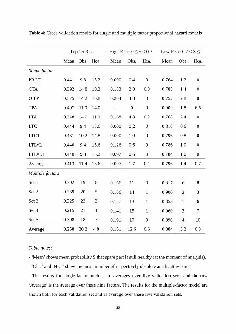
Table 4: Cross-validation results for single and multiple factor proportional hazard models

Top-25 Risk High Risk: 0 ≤ S < 0.3 Low Risk: 0.7 < S ≤ 1

Mean Obs. Hea. Mean Obs. Hea. Mean Obs. Hea.

Single factor

PRCT 0.441 9.8 15.2 0.000 0.4 0 0.764 1.2 0

CTA 0.392 14.8 10.2 0.183 2.8 0.8 0.788 1.4 0

OILP 0.375 14.2 10.8 0.204 4.8 0 0.752 2.8 0

TPA 0.407 11.0 14.0 -- 0 0 0.909 1.8 6.6

LTA 0.348 14.0 11.0 0.168 4.8 0.2 0.768 2.4 0

LTC 0.444 9.4 15.6 0.000 0.2 0 0.816 0.6 0

LTCT 0.431 10.2 14.8 0.000 1.0 0 0.796 0.8 0

LTLvL 0.440 9.4 15.6 0.126 0.6 0 0.786 1.0 0

LTLvLT 0.440 9.8 15.2 0.097 0.6 0 0.784 1.0 0

Average 0.413 11.4 13.6 0.097 1.7 0.1 0.796 1.4 0.7

Multiple factors

Set 1 0.302 19 6 0.166 11 0 0.817 6 8

Set 2 0.239 20 5 0.166 14 1 0.900 3 3

Set 3 0.225 23 2 0.137 13 1 0.853 1 6

Set 4 0.215 21 4 0.141 15 1 0.960 2 7

Set 5 0.308 18 7 0.191 10 0 0.890 4 10

Average 0.258 20.2 4.8 0.161 12.6 0.6 0.884 3.2 6.8

Table notes:

- ‘Mean’ shows mean probability S that spare part is still healthy (at the moment of analysis).

- ‘Obs.’ and ‘Hea.’ show the mean number of respectively obsolete and healthy parts.

- The results for single-factor models are averages over five validation sets, and the row

‘Average’ is the average over these nine factors. The results for the multiple-factor model are

shown both for each validation set and as average over these five validation sets.

35

Figure 1: Kaplan-Meier survival plots of four spare part clusters, labeled 1 for 23 airframe

parts (long dashed line), 2 for 59 electronic parts (short dashed line), 3 for 12 interior parts

(shaded tiny dashed line), and 4 for 272 other parts (continuous line)

36