Embed Size (px)
Citation preview
C H A P T E R 1
Biochemical Reactions
Cells can do lots of wonderful things. Individually they can move, contract, excrete,reproduce, signal or respond to signals, and carry out the energy transactions necessaryfor this activity. Collectively they perform all of the numerous functions of any livingorganism necessary to sustain life. Yet, remarkably, all of what cells do can be describedin terms of a few basic natural laws. The fascination with cells is that although the rulesof behavior are relatively simple, they are applied to an enormously complex network ofinteracting chemicals and substrates. The effort of many lifetimes has been consumedin unraveling just a few of these reaction schemes, and there are many more mysteriesyet to be uncovered.
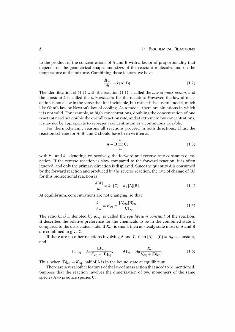
1.1 The Law of Mass Action
The fundamental “law” of a chemical reaction is the law of mass action. This lawdescribes the rate at which chemicals, whether large macromolecules or simpleions, collide and interact to form different chemical combinations. Suppose that twochemicals, say A and B, react upon collision with each other to form product C,
A + Bk−→ C. (1.1)
The rate of this reaction is the rate of accumulation of product, d[C]dt . This rate is the
product of the number of collisions per unit time between the two reactants and theprobability that a collision is sufficiently energetic to overcome the free energy of acti-vation of the reaction. The number of collisions per unit time is taken to be proportional
2 1: Biochemical Reactions
to the product of the concentrations of A and B with a factor of proportionality thatdepends on the geometrical shapes and sizes of the reactant molecules and on thetemperature of the mixture. Combining these factors, we have
d[C]dt= k[A][B]. (1.2)
The identification of (1.2) with the reaction (1.1) is called the law of mass action, andthe constant k is called the rate constant for the reaction. However, the law of massaction is not a law in the sense that it is inviolable, but rather it is a useful model, muchlike Ohm’s law or Newton’s law of cooling. As a model, there are situations in whichit is not valid. For example, at high concentrations, doubling the concentration of onereactant need not double the overall reaction rate, and at extremely low concentrations,it may not be appropriate to represent concentration as a continuous variable.
For thermodynamic reasons all reactions proceed in both directions. Thus, thereaction scheme for A, B, and C should have been written as
A + Bk+−→←−k−
C, (1.3)
with k+ and k− denoting, respectively, the forward and reverse rate constants of re-action. If the reverse reaction is slow compared to the forward reaction, it is oftenignored, and only the primary direction is displayed. Since the quantity A is consumedby the forward reaction and produced by the reverse reaction, the rate of change of [A]for this bidirectional reaction is
d[A]dt= k−[C] − k+[A][B]. (1.4)
At equilibrium, concentrations are not changing, so that
k−k+≡ Keq = [A]eq[B]eq
[C]eq. (1.5)
The ratio k−/k+, denoted by Keq, is called the equilibrium constant of the reaction.It describes the relative preference for the chemicals to be in the combined state Ccompared to the dissociated state. If Keq is small, then at steady state most of A and Bare combined to give C.
If there are no other reactions involving A and C, then [A] + [C] = A0 is constant,and
[C]eq = A0[B]eq
Keq + [B]eq, [A]eq = A0
Keq
Keq + [B]eq. (1.6)
Thus, when [B]eq = Keq, half of A is in the bound state at equilibrium.There are several other features of the law of mass action that need to be mentioned.
Suppose that the reaction involves the dimerization of two monomers of the samespecies A to produce species C,
1.2: Thermodynamics and Rate Constants 3
A + Ak+−→←−k−
C. (1.7)
For every C that is made, two of A are used, and every time C degrades, two copies ofA are produced. As a result, the rate of reaction for A is
d[A]dt= 2k−[C] − 2k+[A]2. (1.8)
However, the rate of production of C is half that of A,
d[C]dt= −1
2d[A]dt
, (1.9)
and the quantity [A]+2[C] is conserved (provided there are no other reactions).In a similar way, with a trimolecular reaction, the rate at which the reaction takes
place is proportional to the product of three concentrations, and three molecules areconsumed in the process, or released in the degradation of product. In real life, thereare probably no truly trimolecular reactions. Nevertheless, there are some situationsin which a reaction might be effectively modeled as trimolecular (Exercise 2).
Unfortunately, the law of mass action cannot be used in all situations, because notall chemical reaction mechanisms are known with sufficient detail. In fact, a vast num-ber of chemical reactions cannot be described by mass action kinetics. Those reactionsthat follow mass action kinetics are called elementary reactions because presumably,they proceed directly from collision of the reactants. Reactions that do not follow massaction kinetics usually proceed by a complex mechanism consisting of several elemen-tary reaction steps. It is often the case with biochemical reactions that the elementaryreaction steps are not known or are very complicated to write down.
1.2 Thermodynamics and Rate Constants
There is a close relationship between the rate constants of a reaction and thermody-namics. The fundamental concept is that of chemical potential, which is the Gibbs freeenergy, G, per mole of a substance. Often, the Gibbs free energy per mole is denotedby μ rather than G. However, because μ has many other uses in this text, we retain thenotation G for the Gibbs free energy.
For a mixture of ideal gases, Xi, the chemical potential of gas i is a function oftemperature, pressure, and concentration,
Gi = G0i (T, P)+ RT ln(xi), (1.10)
where xi is the mole fraction of Xi, R is the universal gas constant, T is the absolutetemperature, and P is the pressure of the gas (in atmospheres); values of these constants,and their units, are given in the appendix. The quantity G0
i (T, P) is the standard freeenergy per mole of the pure ideal gas, i.e., when the mole fraction of the gas is 1. Note
4 1: Biochemical Reactions
that, since xi ≤ 1, the free energy of an ideal gas in a mixture is always less than thatof the pure ideal gas. The total Gibbs free energy of the mixture is
G =∑
i
niGi, (1.11)
where ni is the number of moles of gas i.The theory of Gibbs free energy in ideal gases can be extended to ideal dilute
solutions. By redefining the standard Gibbs free energy to be the free energy at aconcentration of 1 M, i.e., 1 mole per liter, we obtain
G = G0 + RT ln(c), (1.12)
where the concentration, c, is in units of moles per liter. The standard free energy, G0,is obtained by measuring the free energy for a dilute solution and then extrapolatingto c = 1 M. For biochemical applications, the dependence of free energy on pressureis ignored, and the pressure is assumed to be 1 atm, while the temperature is taken tobe 25◦C. Derivations of these formulas can be found in physical chemistry textbookssuch as Levine (2002) and Castellan (1971).
For nonideal solutions, such as are typical in cells, the free energy formula (1.12)should use the chemical activity of the solute rather than its concentration. The re-lationship between chemical activity a and concentration is nontrivial. However, fordilute concentrations, they are approximately equal.
Since the free energy is a potential, it denotes the preference of one state comparedto another. Consider, for example, the simple reaction
A −→ B. (1.13)
The change in chemical potential�G is defined as the difference between the chemicalpotential for state B (the product), denoted by GB, and the chemical potential for stateA (the reactant), denoted by GA,
�G = GB −GA
= G0B −G0
A + RT ln([B])− RT ln([A])= �G0 + RT ln([B]/[A]). (1.14)
The sign of�G is important, which is why it is defined with only one reaction directionshown, even though we know that the back reaction also occurs. In fact, there is awonderful opportunity for confusion here, since there is no obvious way to decidewhich is the forward and which is the backward direction for a given reaction. If�G < 0, then state B is preferred to state A, and the reaction tends to convert A intoB, whereas, if �G > 0, then state A is preferred to state B, and the reaction tends toconvert B into A. Equilibrium occurs when neither state is preferred, so that �G = 0,in which case
[B]eq
[A]eq= e
−�G0RT . (1.15)
1.2: Thermodynamics and Rate Constants 5
Expressing this reaction in terms of forward and backward reaction rates,
Ak+−→←−k−
B, (1.16)
we find that in steady state, k+[A]eq = k−[B]eq, so that
[A]eq
[B]eq= k−
k+= Keq. (1.17)
Combining this with (1.15), we observe that
Keq = e�G0RT . (1.18)
In other words, the more negative the difference in standard free energy, the greaterthe propensity for the reaction to proceed from left to right, and the smaller is Keq.Notice, however, that this gives only the ratio of rate constants, and not their individualamplitudes. We learn nothing about whether a reaction is fast or slow from the changein free energy.
Similar relationships hold when there are multiple components in the reaction.Consider, for example, the more complex reaction
αA + βB −→ γC+ δD. (1.19)
The change of free energy for this reaction is defined as
�G = γGC + δGD − αGA − βGB
= γG0C + δG0
D − αG0A − βG0
B + RT ln( [C]γ [D]δ[A]α[B]β
)
= �G0 + RT ln( [C]γ [D]δ[A]α[B]β
), (1.20)
and at equilibrium,
�G0 = RT ln
( [A]αeq[B]βeq
[C]γeq[D]δeq
)= RT ln(Keq). (1.21)
An important example of such a reaction is the hydrolysis of adenosine triphosphate(ATP) to adenosine diphosphate (ADP) and inorganic phosphate Pi, represented by thereaction
ATP −→ ADP+ Pi. (1.22)
The standard free energy change for this reaction is
�G0 = G0ADP +G0
Pi−G0
ATP = −31.0 kJ mol−1, (1.23)
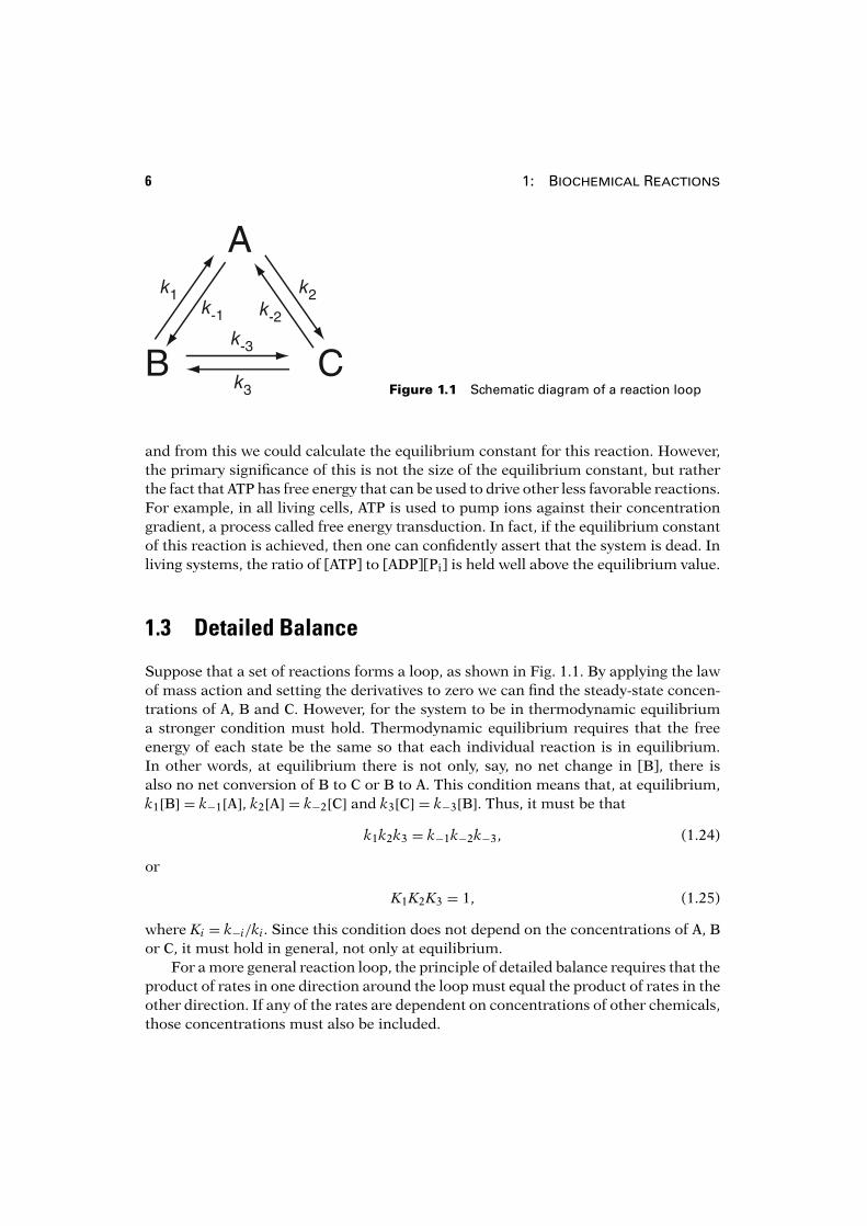
6 1: Biochemical Reactions
A
B C
k1 k2
k3
k-1 k-2
k-3
Figure 1.1 Schematic diagram of a reaction loop
and from this we could calculate the equilibrium constant for this reaction. However,the primary significance of this is not the size of the equilibrium constant, but ratherthe fact that ATP has free energy that can be used to drive other less favorable reactions.For example, in all living cells, ATP is used to pump ions against their concentrationgradient, a process called free energy transduction. In fact, if the equilibrium constantof this reaction is achieved, then one can confidently assert that the system is dead. Inliving systems, the ratio of [ATP] to [ADP][Pi] is held well above the equilibrium value.
1.3 Detailed Balance
Suppose that a set of reactions forms a loop, as shown in Fig. 1.1. By applying the lawof mass action and setting the derivatives to zero we can find the steady-state concen-trations of A, B and C. However, for the system to be in thermodynamic equilibriuma stronger condition must hold. Thermodynamic equilibrium requires that the freeenergy of each state be the same so that each individual reaction is in equilibrium.In other words, at equilibrium there is not only, say, no net change in [B], there isalso no net conversion of B to C or B to A. This condition means that, at equilibrium,k1[B] = k−1[A], k2[A] = k−2[C] and k3[C] = k−3[B]. Thus, it must be that
k1k2k3 = k−1k−2k−3, (1.24)
or
K1K2K3 = 1, (1.25)
where Ki = k−i/ki. Since this condition does not depend on the concentrations of A, Bor C, it must hold in general, not only at equilibrium.
For a more general reaction loop, the principle of detailed balance requires that theproduct of rates in one direction around the loop must equal the product of rates in theother direction. If any of the rates are dependent on concentrations of other chemicals,those concentrations must also be included.
1.4: Enzyme Kinetics 7
1.4 Enzyme Kinetics
To see where some of the more complicated reaction schemes come from, we consider areaction that is catalyzed by an enzyme. Enzymes are catalysts (generally proteins) thathelp convert other molecules called substrates into products, but they themselves arenot changed by the reaction. Their most important features are catalytic power, speci-ficity, and regulation. Enzymes accelerate the conversion of substrate into product bylowering the free energy of activation of the reaction. For example, enzymes may aidin overcoming charge repulsions and allowing reacting molecules to come into contactfor the formation of new chemical bonds. Or, if the reaction requires breaking of anexisting bond, the enzyme may exert a stress on a substrate molecule, rendering aparticular bond more easily broken. Enzymes are particularly efficient at speeding upbiological reactions, giving increases in speed of up to 10 million times or more. Theyare also highly specific, usually catalyzing the reaction of only one particular substrateor closely related substrates. Finally, they are typically regulated by an enormouslycomplicated set of positive and negative feedbacks, thus allowing precise control overthe rate of reaction. A detailed presentation of enzyme kinetics, including many differ-ent kinds of models, can be found in Dixon and Webb (1979), the encyclopedic Segel(1975) or Kernevez (1980). Here, we discuss only some of the simplest models.
One of the first things one learns about enzyme reactions is that they do not followthe law of mass action directly. For, as the concentration of substrate (S) is increased,the rate of the reaction increases only to a certain extent, reaching a maximal reactionvelocity at high substrate concentrations. This is in contrast to the law of mass action,which, when applied directly to the reaction of S with the enzyme E
S+ E −→ P+ E
predicts that the reaction velocity increases linearly as [S] increases.A model to explain the deviation from the law of mass action was first proposed
by Michaelis and Menten (1913). In their reaction scheme, the enzyme E converts thesubstrate S into the product P through a two-step process. First E combines with Sto form a complex C which then breaks down into the product P releasing E in theprocess. The reaction scheme is represented schematically by
S+ Ek1−→←−
k−1
Ck2−→←−
k−2
P+ E.
Although all reactions must be reversible, as shown here, reaction rates are typicallymeasured under conditions where P is continually removed, which effectively preventsthe reverse reaction from occurring. Thus, it often suffices to assume that no reversereaction occurs. For this reason, the reaction is usually written as
S+ Ek1−→←−
k−1
Ck2−→P+ E.
The reversible case is considered in Section 1.4.5.
8 1: Biochemical Reactions
There are two similar, but not identical, ways to analyze this equation; theequilibrium approximation, and the quasi-steady-state approximation. Because thesemethods give similar results it is easy to confuse them, so it is important to understandtheir differences.
We begin by defining s = [S], c = [C], e = [E], and p = [P]. The law of mass actionapplied to this reaction mechanism gives four differential equations for the rates ofchange of s, c, e, and p,
dsdt= k−1c− k1se, (1.26)
dedt= (k−1 + k2)c− k1se, (1.27)
dcdt= k1se− (k2 + k−1)c, (1.28)
dpdt= k2c. (1.29)
Note that p can be found by direct integration, and that there is a conserved quantitysince de
dt + dcdt = 0, so that e+ c = e0, where e0 is the total amount of available enzyme.
1.4.1 The Equilibrium Approximation
In their original analysis, Michaelis and Menten assumed that the substrate is ininstantaneous equilibrium with the complex, and thus
k1se = k−1c. (1.30)
Since e+ c = e0, we find that
c = e0sK1 + s
, (1.31)
where K1 = k−1/k1. Hence, the velocity, V , of the reaction, i.e., the rate at which theproduct is formed, is given by
V = dpdt= k2c = k2e0s
K1 + s= Vmaxs
K1 + s, (1.32)
where Vmax = k2e0 is the maximum reaction velocity, attained when all the enzyme iscomplexed with the substrate.
At small substrate concentrations, the reaction rate is linear, at a rate proportionalto the amount of available enzyme e0. At large concentrations, however, the reactionrate saturates to Vmax, so that the maximum rate of the reaction is limited by theamount of enzyme present and the dissociation rate constant k2. For this reason, the
dissociation reaction Ck2−→P+ E is said to be rate limiting for this reaction. At s = K1,
the reaction rate is half that of the maximum.It is important to note that (1.30) cannot be exactly correct at all times; if it were,
then according to (1.26) substrate would not be used up, and product would not be
1.4: Enzyme Kinetics 9
formed. This points out the fact that (1.30) is an approximation. It also illustrates theneed for a systematic way to make approximate statements, so that one has an idea ofthe magnitude and nature of the errors introduced in making such an approximation.
It is a common mistake with the equilibrium approximation to conclude that since(1.30) holds, it must be that ds
dt = 0, which if this is true, implies that no substrate isbeing used up, nor product produced. Furthermore, it appears that if (1.30) holds, thenit must be (from (1.28)) that dc
dt = −k2c, which is also false. Where is the error here?The answer lies with the fact that the equilibrium approximation is equivalent to
the assumption that the reaction (1.26) is a very fast reaction, faster than others, ormore precisely, that k−1 � k2. Adding (1.26) and (1.28), we find that
dsdt+ dc
dt= −k2c, (1.33)
expressing the fact that the total quantity s + c changes on a slower time scale. Nowwhen we use that c = e0s
Ks+s , we learn that
ddt
(s+ e0s
K1 + s
)= −k2
e0sK1 + s
, (1.34)
and thus,
dsdt
(1+ e0K1
(K1 + s)2
)= −k2
e0sK1 + s
, (1.35)
which specifies the rate at which s is consumed.This way of simplifying reactions by using an equilibrium approximation is used
many times throughout this book, and is an extremely important technique, par-ticularly in the analysis of Markov models of ion channels, pumps and exchangers(Chapters 2 and 3). A more mathematically systematic description of this approach isleft for Exercise 20.
1.4.2 The Quasi-Steady-State Approximation
An alternative analysis of an enzymatic reaction was proposed by Briggs and Haldane(1925) who assumed that the rates of formation and breakdown of the complex wereessentially equal at all times (except perhaps at the beginning of the reaction, as thecomplex is “filling up”). Thus, dc/dt should be approximately zero.
To give this approximation a systematic mathematical basis, it is useful to introducedimensionless variables
σ = ss0
, x = ce0
, τ = k1e0t, κ = k−1 + k2
k1s0, ε = e0
s0, α = k−1
k1s0, (1.36)
10 1: Biochemical Reactions
in terms of which we obtain the system of two differential equations
dσdτ= −σ + x(σ + α), (1.37)
εdxdτ= σ − x(σ + κ). (1.38)
There are usually a number of ways that a system of differential equations can benondimensionalized. This nonuniqueness is often a source of great confusion, as it isoften not obvious which choice of dimensionless variables and parameters is “best.” InSection 1.6 we discuss this difficult problem briefly.
The remarkable effectiveness of enzymes as catalysts of biochemical reactions isreflected by their small concentrations needed compared to the concentrations of thesubstrates. For this model, this means that ε is small, typically in the range of 10−2
to 10−7. Therefore, the reaction (1.38) is fast, equilibrates rapidly and remains innear-equilibrium even as the variable σ changes. Thus, we take the quasi-steady-stateapproximation ε dx
dτ = 0. Notice that this is not the same as taking dxdτ = 0. However,
because of the different scaling of x and c, it is equivalent to taking dcdt = 0 as suggested
in the introductory paragraph.One useful way of looking at this system is as follows; since
dxdτ= σ − x(σ + κ)
ε, (1.39)
dx/dτ is large everywhere, except where σ−x(σ+κ) is small, of approximately the samesize as ε. Now, note that σ − x(σ + κ) = 0 defines a curve in the σ , x phase plane, calledthe slow manifold (as illustrated in the right panel of Fig. 1.14). If the solution startsaway from the slow manifold, dx/dτ is initially large, and the solution moves rapidlyto the vicinity of the slow manifold. The solution then moves along the slow manifoldin the direction defined by the equation for σ ; in this case, σ is decreasing, and so thesolution moves to the left along the slow manifold.
Another way of looking at this model is to notice that the reaction of x is an ex-ponential process with time constant at least as large as κ
ε. To see this we write (1.38)
as
εdxdτ+ κx = σ(1− x). (1.40)
Thus, the variable x “tracks” the steady state with a short delay.It follows from the quasi-steady-state approximation that
x = σ
σ + κ , (1.41)
dσdτ= − qσ
σ + κ , (1.42)
1.4: Enzyme Kinetics 11
where q = κ − α = k2k1s0
. Equation (1.42) describes the rate of uptake of the substrate
and is called a Michaelis–Menten law. In terms of the original variables, this law is
V = dpdt= −ds
dt= k2e0s
s+ Km= Vmaxs
s+ Km, (1.43)
where Km = k−1+k2k1
. In quasi-steady state, the concentration of the complex satisfies
c = e0ss+ Km
. (1.44)
Note the similarity between (1.32) and (1.43), the only difference being that the equi-librium approximation uses K1, while the quasi-steady-state approximation uses Km.Despite this similarity of form, it is important to keep in mind that the two resultsare based on different approximations. The equilibrium approximation assumes thatk−1 � k2 whereas the quasi-steady-state approximation assumes that ε � 1. No-tice, that if k−1 � k2, then Km ≈ K1, so that the two approximations give similarresults.
As with the law of mass action, the Michaelis–Menten law (1.43) is not universallyapplicable but is a useful approximation. It may be applicable even if ε = e0/s0 is notsmall (see, for example, Exercise 14), and in model building it is often invoked withoutregard to the underlying assumptions.
While the individual rate constants are difficult to measure experimentally, the ratioKm is relatively easy to measure because of the simple observation that (1.43) can bewritten in the form
1V= 1
Vmax+ Km
Vmax
1s
. (1.45)
In other words, 1/V is a linear function of 1/s. Plots of this double reciprocal curve arecalled Lineweaver–Burk plots, and from such (experimentally determined) plots, Vmax
and Km can be estimated.Although a Lineweaver–Burk plot makes it easy to determine Vmax and Km from
reaction rate measurements, it is not a simple matter to determine the reaction rateas a function of substrate concentration during the course of a single experiment.Substrate concentrations usually cannot be measured with sufficient accuracy or timeresolution to permit the calculation of a reliable derivative. In practice, since it is moreeasily measured, the initial reaction rate is determined for a range of different initialsubstrate concentrations.
An alternative method to determine Km and Vmax from experimental data is the di-rect linear plot (Eisenthal and Cornish-Bowden, 1974; Cornish-Bowden and Eisenthal,1974). First we write (1.43) in the form
Vmax = V + Vs
Km, (1.46)
12 1: Biochemical Reactions
and then treat Vmax and Km as variables for each experimental measurement of V and s.(Recall that typically only the initial substrate concentration and initial velocity areused.) Then a plot of the straight line of Vmax against Km can be made. Repeating thisfor a number of different initial substrate concentrations and velocities gives a familyof straight lines, which, in an ideal world free from experimental error, intersect at thesingle point Vmax and Km for that reaction. In reality, experimental error precludes anexact intersection, but Vmax and Km can be estimated from the median of the pairwiseintersections.
1.4.3 Enzyme Inhibition
An enzyme inhibitor is a substance that inhibits the catalytic action of the enzyme.Enzyme inhibition is a common feature of enzyme reactions, and is an importantmeans by which the activity of enzymes is controlled. Inhibitors come in many differenttypes. For example, irreversible inhibitors, or catalytic poisons, decrease the activity ofthe enzyme to zero. This is the method of action of cyanide and many nerve gases.For this discussion, we restrict our attention to competitive inhibitors and allostericinhibitors.
To understand the distinction between competitive and allosteric inhibition, it isuseful to keep in mind that an enzyme molecule is usually a large protein, considerablylarger than the substrate molecule whose reaction is catalyzed. Embedded in the largeenzyme protein are one or more active sites, to which the substrate can bind to form thecomplex. In general, an enzyme catalyzes a single reaction of substrates with similarstructures. This is believed to be a steric property of the enzyme that results from thethree-dimensional shape of the enzyme allowing it to fit in a “lock-and-key” fashionwith a corresponding substrate molecule.
If another molecule has a shape similar enough to that of the substrate molecule,it may also bind to the active site, preventing the binding of a substrate molecule, thusinhibiting the reaction. Because the inhibitor competes with the substrate moleculefor the active site, it is called a competitive inhibitor.
However, because the enzyme molecule is large, it often has other binding sites,distinct from the active site, the binding of which affects the activity of the enzymeat the active site. These binding sites are called allosteric sites (from the Greek for“another solid”) to emphasize that they are structurally different from the catalyticactive sites. They are also called regulatory sites to emphasize that the catalytic activityof the protein is regulated by binding at this allosteric site. The ligand (any moleculethat binds to a specific site on a protein, from Latin ligare, to bind) that binds at theallosteric site is called an effector or modifier, which, if it increases the activity of theenzyme, is called an allosteric activator, while if it decreases the activity of the enzyme,is called an allosteric inhibitor. The allosteric effect is presumed to arise because of aconformational change of the enzyme, that is, a change in the folding of the polypeptidechain, called an allosteric transition.
1.4: Enzyme Kinetics 13
Competitive InhibitionIn the simplest example of a competitive inhibitor, the reaction is stopped when theinhibitor is bound to the active site of the enzyme. Thus,
S+ Ek1−→←−
k−1
C1k2−→E+ P,
E+ Ik3−→←−
k−3
C2.
Using the law of mass action we find
dsdt= −k1se+ k−1c1, (1.47)
didt= −k3ie+ k−3c2, (1.48)
dc1
dt= k1se− (k−1 + k2)c1, (1.49)
dc2
dt= k3ie− k−3c2. (1.50)
where s = [S], c1 = [C1], and c2 = [C2]. We know that e+ c1 + c2 = e0, so an equationfor the dynamics of e is superfluous. As before, it is not necessary to write an equationfor the accumulation of the product. To be systematic, the next step is to introducedimensionless variables, and identify those reactions that are rapid and equilibraterapidly to their quasi-steady states. However, from our previous experience (or from acalculation on a piece of scratch paper), we know, assuming the enzyme-to-substrateratios are small, that the fast equations are those for c1 and c2. Hence, the quasi-steadystates are found by (formally) setting dc1/dt = dc2/dt = 0 and solving for c1 and c2.Recall that this does not mean that c1 and c2 are unchanging, rather that they arechanging in quasi-steady-state fashion, keeping the right-hand sides of these equationsnearly zero. This gives
c1 = Kie0sKmi+ Kis+ KmKi
, (1.51)
c2 = Kme0iKmi+ Kis+ KmKi
, (1.52)
where Km = k−1+k2k1
, Ki = k−3/k3. Thus, the velocity of the reaction is
V = k2c1 = k2e0sKi
Kmi+ Kis+ KmKi= Vmaxs
s+ Km(1+ i/Ki). (1.53)
Notice that the effect of the inhibitor is to increase the effective equilibrium constant ofthe enzyme by the factor 1+ i/Ki, from Km to Km(1+ i/Ki), thus decreasing the velocityof reaction, while leaving the maximum velocity unchanged.
14 1: Biochemical Reactions
E ES
EI EIS
E + Pk1s
k-1
k1s
k-1
k3i k-3 k3i k-3
k2
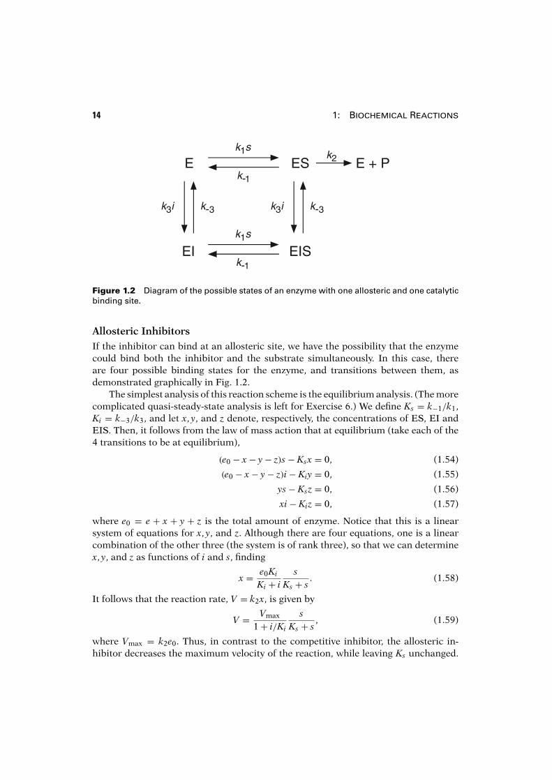
Figure 1.2 Diagram of the possible states of an enzyme with one allosteric and one catalyticbinding site.
Allosteric InhibitorsIf the inhibitor can bind at an allosteric site, we have the possibility that the enzymecould bind both the inhibitor and the substrate simultaneously. In this case, thereare four possible binding states for the enzyme, and transitions between them, asdemonstrated graphically in Fig. 1.2.
The simplest analysis of this reaction scheme is the equilibrium analysis. (The morecomplicated quasi-steady-state analysis is left for Exercise 6.) We define Ks = k−1/k1,Ki = k−3/k3, and let x, y, and z denote, respectively, the concentrations of ES, EI andEIS. Then, it follows from the law of mass action that at equilibrium (take each of the4 transitions to be at equilibrium),
(e0 − x− y− z)s− Ksx = 0, (1.54)
(e0 − x− y− z)i− Kiy = 0, (1.55)
ys− Ksz = 0, (1.56)
xi− Kiz = 0, (1.57)
where e0 = e + x + y + z is the total amount of enzyme. Notice that this is a linearsystem of equations for x, y, and z. Although there are four equations, one is a linearcombination of the other three (the system is of rank three), so that we can determinex, y, and z as functions of i and s, finding
x = e0Ki
Ki + is
Ks + s. (1.58)
It follows that the reaction rate, V = k2x, is given by
V = Vmax
1+ i/Ki
sKs + s
, (1.59)
where Vmax = k2e0. Thus, in contrast to the competitive inhibitor, the allosteric in-hibitor decreases the maximum velocity of the reaction, while leaving Ks unchanged.
1.4: Enzyme Kinetics 15
(The situation is more complicated if the quasi-steady-state approximation is used, andno such simple conclusion follows.)
1.4.4 Cooperativity
For many enzymes, the reaction velocity is not a simple hyperbolic curve, as predictedby the Michaelis–Menten model, but often has a sigmoidal character. This can re-sult from cooperative effects, in which the enzyme can bind more than one substratemolecule but the binding of one substrate molecule affects the binding of subsequentones.
Much of the original theoretical work on cooperative behavior was stimulated bythe properties of hemoglobin, and this is often the context in which cooperativity isdiscussed. A detailed discussion of hemoglobin and oxygen binding is given in Chapter13, while here cooperativity is discussed in more general terms.
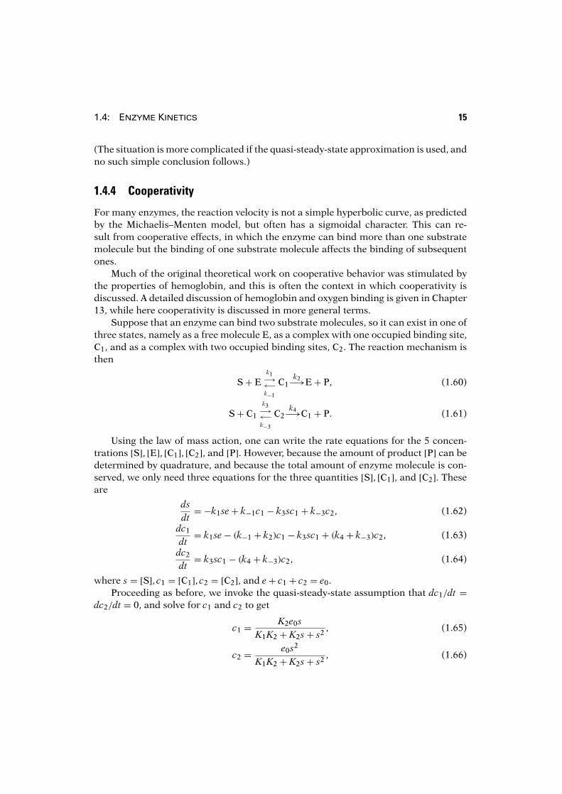
Suppose that an enzyme can bind two substrate molecules, so it can exist in one ofthree states, namely as a free molecule E, as a complex with one occupied binding site,C1, and as a complex with two occupied binding sites, C2. The reaction mechanism isthen
S+ Ek1−→←−
k−1
C1k2−→E+ P, (1.60)
S+ C1
k3−→←−k−3
C2k4−→C1 + P. (1.61)
Using the law of mass action, one can write the rate equations for the 5 concen-trations [S], [E], [C1], [C2], and [P]. However, because the amount of product [P] can bedetermined by quadrature, and because the total amount of enzyme molecule is con-served, we only need three equations for the three quantities [S], [C1], and [C2]. Theseare
dsdt= −k1se+ k−1c1 − k3sc1 + k−3c2, (1.62)
dc1
dt= k1se− (k−1 + k2)c1 − k3sc1 + (k4 + k−3)c2, (1.63)
dc2
dt= k3sc1 − (k4 + k−3)c2, (1.64)
where s = [S], c1 = [C1], c2 = [C2], and e+ c1 + c2 = e0.Proceeding as before, we invoke the quasi-steady-state assumption that dc1/dt =
dc2/dt = 0, and solve for c1 and c2 to get
c1 = K2e0sK1K2 + K2s+ s2 , (1.65)
c2 = e0s2
K1K2 + K2s+ s2 , (1.66)
16 1: Biochemical Reactions
where K1 = k−1+k2k1
and K2 = k4+k−3k3
. The reaction velocity is thus given by
V = k2c1 + k4c2 = (k2K2 + k4s)e0sK1K2 + K2s+ s2 . (1.67)
Use of the equilibrium approximation to simplify this reaction scheme gives, asexpected, similar results, in which the formula looks the same, but with differentdefinitions of K1 and K2 (Exercise 10).
It is instructive to examine two extreme cases. First, if the binding sites act inde-pendently and identically, then k1 = 2k3 = 2k+, 2k−1 = k−3 = 2k− and 2k2 = k4, wherek+ and k− are the forward and backward reaction rates for the individual binding sites.The factors of 2 occur because two identical binding sites are involved in the reaction,doubling the amount of the reactant. In this case,
V = 2k2e0(K + s)sK2 + 2Ks+ s2 = 2
k2e0sK + s
, (1.68)
where K = k−+k2k+ is the Km of the individual binding site. As expected, the rate of
reaction is exactly twice that for the individual binding site.In the opposite extreme, suppose that the binding of the first substrate molecule is
slow, but that with one site bound, binding of the second is fast (this is large positivecooperativity). This can be modeled by letting k3 →∞ and k1 → 0, while keeping k1k3
constant, in which case K2 → 0 and K1 →∞ while K1K2 is constant. In this limit, thevelocity of the reaction is
V = k4e0s2
K2m + s2 =
Vmaxs2
K2m + s2 , (1.69)
where K2m = K1K2, and Vmax = k4e0.
In general, if n substrate molecules can bind to the enzyme, there are n equilibriumconstants, K1 through Kn. In the limit as Kn → 0 and K1 → ∞ while keeping K1Kn
fixed, the rate of reaction is
V = Vmaxsn
Knm + sn , (1.70)
where Knm = �n
i=1Ki. This rate equation is known as the Hill equation. Typically, theHill equation is used for reactions whose detailed intermediate steps are not knownbut for which cooperative behavior is suspected. The exponent n and the parametersVmax and Km are usually determined from experimental data. Observe that
n ln s = n ln Km + ln(
VVmax − V
), (1.71)
so that a plot of ln( VVmax−V ) against ln s (called a Hill plot) should be a straight line of
slope n. Although the exponent n suggests an n-step process (with n binding sites), inpractice it is not unusual for the best fit for n to be noninteger.
An enzyme can also exhibit negative cooperativity (Koshland and Hamadani, 2002),in which the binding of the first substrate molecule decreases the rate of subsequent
1.4: Enzyme Kinetics 17
1.6
1.4
1.2
1.0
0.8
0.6
0.4
0.2
0.0
Rea
ctio
n ve
loci
ty, V
2.01.51.00.50.0Substrate concentration, s
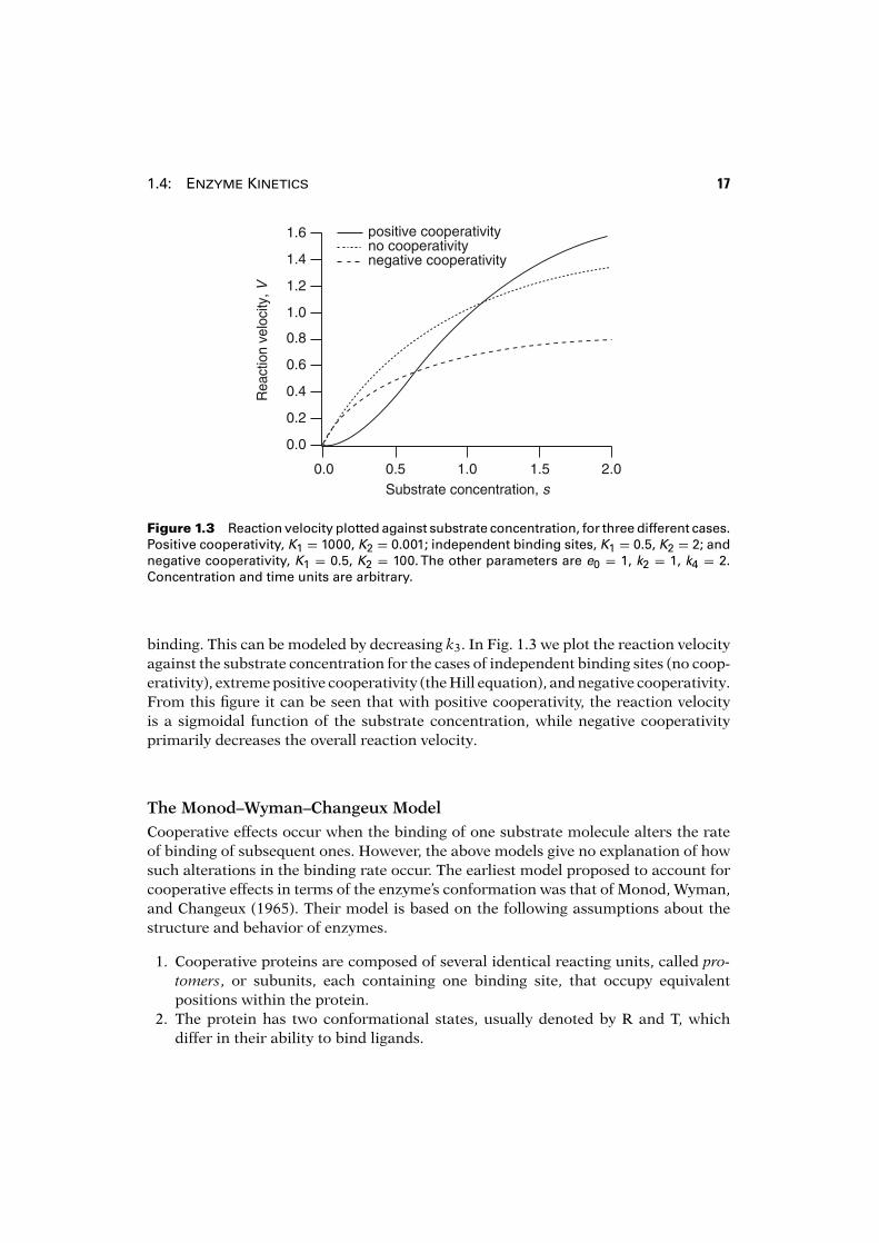
positive cooperativity no cooperativity negative cooperativity
Figure 1.3 Reaction velocity plotted against substrate concentration, for three different cases.Positive cooperativity, K1 = 1000, K2 = 0.001; independent binding sites, K1 = 0.5, K2 = 2; andnegative cooperativity, K1 = 0.5, K2 = 100. The other parameters are e0 = 1, k2 = 1, k4 = 2.Concentration and time units are arbitrary.
binding. This can be modeled by decreasing k3. In Fig. 1.3 we plot the reaction velocityagainst the substrate concentration for the cases of independent binding sites (no coop-erativity), extreme positive cooperativity (the Hill equation), and negative cooperativity.From this figure it can be seen that with positive cooperativity, the reaction velocityis a sigmoidal function of the substrate concentration, while negative cooperativityprimarily decreases the overall reaction velocity.
The Monod–Wyman–Changeux ModelCooperative effects occur when the binding of one substrate molecule alters the rateof binding of subsequent ones. However, the above models give no explanation of howsuch alterations in the binding rate occur. The earliest model proposed to account forcooperative effects in terms of the enzyme’s conformation was that of Monod, Wyman,and Changeux (1965). Their model is based on the following assumptions about thestructure and behavior of enzymes.
1. Cooperative proteins are composed of several identical reacting units, called pro-tomers, or subunits, each containing one binding site, that occupy equivalentpositions within the protein.
2. The protein has two conformational states, usually denoted by R and T, whichdiffer in their ability to bind ligands.
18 1: Biochemical Reactions
R0 R1 R2
2sk1
k-1
sk1
2k-1
T0 T1 T2
2sk3
k-3
sk3
2k-3
k2 k-2
Figure 1.4 Diagram of the states ofthe protein, and the possible transi-tions, in a six-state Monod–Wyman–Changeux model.
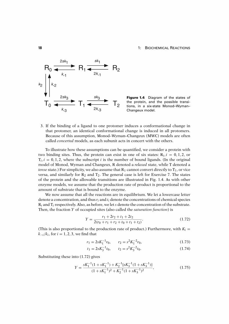
3. If the binding of a ligand to one protomer induces a conformational change inthat protomer, an identical conformational change is induced in all protomers.Because of this assumption, Monod–Wyman–Changeux (MWC) models are oftencalled concerted models, as each subunit acts in concert with the others.
To illustrate how these assumptions can be quantified, we consider a protein withtwo binding sites. Thus, the protein can exist in one of six states: Ri, i = 0, 1, 2, orTi, i = 0, 1, 2, where the subscript i is the number of bound ligands. (In the originalmodel of Monod, Wyman and Changeux, R denoted a relaxed state, while T denoted atense state.) For simplicity, we also assume that R1 cannot convert directly to T1, or viceversa, and similarly for R2 and T2. The general case is left for Exercise 7. The statesof the protein and the allowable transitions are illustrated in Fig. 1.4. As with otherenzyme models, we assume that the production rate of product is proportional to theamount of substrate that is bound to the enzyme.
We now assume that all the reactions are in equilibrium. We let a lowercase letterdenote a concentration, and thus ri and ti denote the concentrations of chemical speciesRi and Ti respectively. Also, as before, we let s denote the concentration of the substrate.Then, the fraction Y of occupied sites (also called the saturation function) is
Y = r1 + 2r2 + t1 + 2t22(r0 + r1 + r2 + t0 + t1 + t2)
. (1.72)
(This is also proportional to the production rate of product.) Furthermore, with Ki =k−i/ki, for i = 1, 2, 3, we find that
r1 = 2sK−11 r0, r2 = s2K−2
1 r0, (1.73)
t1 = 2sK−13 t0, t2 = s2K−2
3 t0. (1.74)
Substituting these into (1.72) gives
Y = sK−11 (1+ sK−1
1 )+ K−12 [sK−1
3 (1+ sK−13 )]
(1+ sK−11 )2 + K−1
2 (1+ sK−13 )2
, (1.75)
1.4: Enzyme Kinetics 19
where we have used that r0/t0 = K2. More generally, if there are n binding sites, then
Y = sK−11 (1+ sK−1
1 )n−1 + K−12 [sK−1
3 (1+ sK−13 )n−1]
(1+ sK−11 )n + K−1
2 (1+ sK−13 )n
. (1.76)
In general, Y is a sigmoidal function of s.It is not immediately apparent how cooperative binding kinetics arises from this
model. After all, each binding site in the R conformation is identical, as is each bindingsite in the T conformation. In order to get cooperativity it is necessary that the bindingaffinity of the R conformation be different from that of the T conformation. In thespecial case that the binding affinities of the R and T conformations are equal (i.e.,K1 = K3 = K, say) the binding curve (1.76) reduces to
Y = sK + s
, (1.77)
which is simply noncooperative Michaelis–Menten kinetics.Suppose that one conformation, T say, binds the substrate with a higher affinity
than does R. Then, when the substrate concentration increases, T0 is pushed throughto T1 faster than R0 is pushed to R1, resulting in an increase in the amount of substratebound to the T state, and thus increased overall binding of substrate. Hence thecooperative behavior of the model.
If K2 = ∞, so that only one conformation exists, then once again the saturationcurve reduces to the Michaelis–Menten equation, Y = s/(s + K1). Hence each con-formation, by itself, has noncooperative Michaelis–Menten binding kinetics. It is onlywhen the overall substrate binding can be biased to one conformation or the other thatcooperativity appears.
Interestingly, MWC models cannot exhibit negative cooperativity. No matterwhether K1 > K3 or vice versa, the binding curve always exhibits positive cooperativity.
The Koshland–Nemethy–Filmer modelOne alternative to the MWC model is that proposed by Koshland, Nemethy and Filmerin 1966 (the KNF model). Instead of requiring that all subunit transitions occur inconcert, as in the MWC model, the KNF model assumes that substrate binding to onesubunit causes a conformational change in that subunit only, and that this conforma-tional change causes a change in the binding affinity of the neighboring subunits. Thus,in the KNF model, each subunit can be in a different conformational state, and tran-sitions from one state to the other occur sequentially as more substrate is bound. Forthis reason KNF models are often called sequential models. The increased generalityof the KNF model allows for the possibility of negative cooperativity, as the binding toone subunit can decrease the binding affinity of its neighbors.
When binding shows positive cooperativity, it has proven difficult to distinguishbetween the MWC and KNF models on the basis of experimental data. In one of themost intensely studied cooperative mechanisms, that of oxygen binding to hemoglobin,
20 1: Biochemical Reactions
there is experimental evidence for both models, and the actual mechanism is probablya combination of both.
There are many other models of enzyme cooperativity, and the interested reader isreferred to Dixon and Webb (1979) for a comprehensive discussion and comparison ofother models in the literature.
1.4.5 Reversible Enzyme Reactions
Since all enzyme reactions are reversible, a general understanding of enzyme kineticsmust take this reversibility into account. In this case, the reaction scheme is
S+ Ek1−→←−
k−1
Ck2−→←−
k−2
P+ E.
Proceeding as usual, we let e+ c = e0 and make the quasi-steady-state assumption
0 = dcdt= k1s(e0 − c)− (k−1 + k2)c+ k−2p(e0 − c), (1.78)
from which it follows that
c = e0(k1s+ k−2p)k1s+ k−2p+ k−1 + k2
. (1.79)
The reaction velocity, V = dPdt = k2c− k−2pe, can then be calculated to be
V = e0k1k2s− k−1k−2p
k1s+ k−2p+ k−1 + k2. (1.80)
When p is small (e.g., if product is continually removed), the reverse reaction isnegligible and we get the previous answer (1.43).
In contrast to the irreversible case, the equilibrium and quasi-steady-state assump-tions for reversible enzyme kinetics give qualitatively different answers. If we assumethat S, E, and C are in fast equilibrium (instead of assuming that C is at quasi-steadystate) we get
k1s(e0 − c) = k−1c, (1.81)
from which it follows that
V = k2c− k−2p(e0 − c) = e0k1k2s− k−1k−2p
k1s+ k−1. (1.82)
Comparing this to (1.80), we see that the quasi-steady-state assumption gives addi-tional terms in the denominator involving the product p. These differences result fromthe assumption underlying the fast-equilibrium assumption, that k−1 and k1 are bothsubstantially larger than k−2 and k2, respectively. Which of these approximations isbest depends, of course, on the details of the reaction.
Calculation of the equations for a reversible enzyme reaction in which the enzymehas multiple binding sites is left for the exercises (Exercise 11).
1.4: Enzyme Kinetics 21
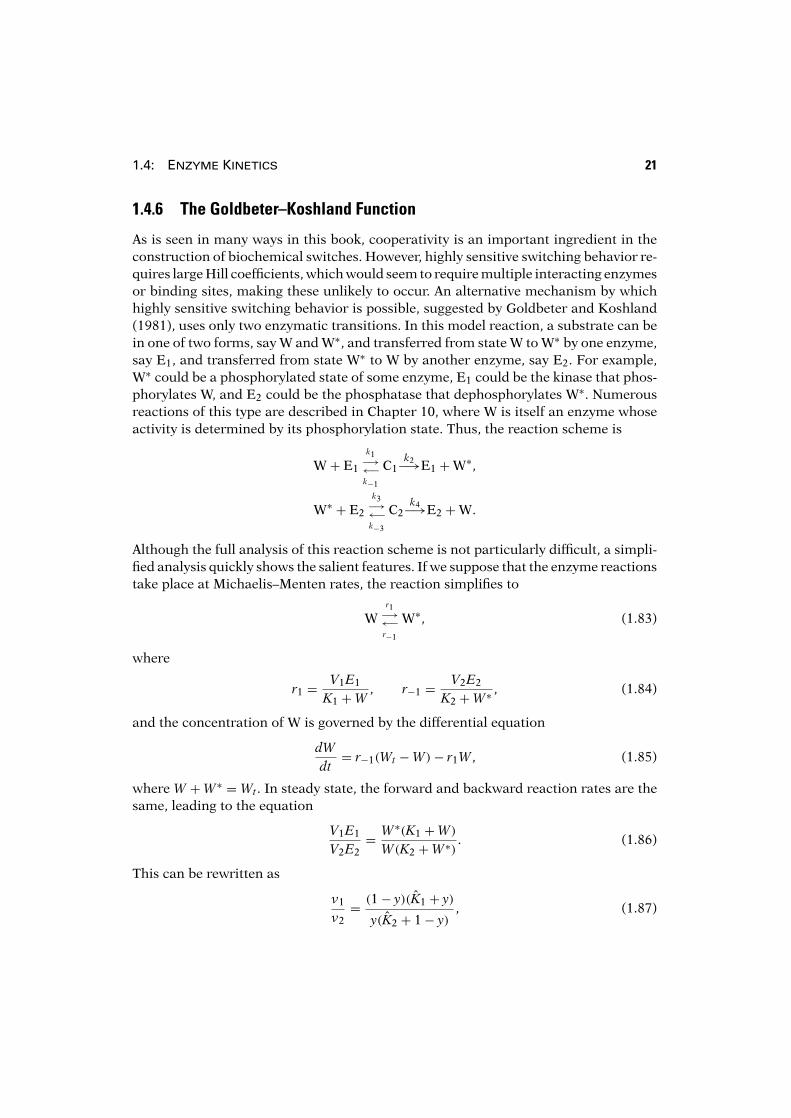
1.4.6 The Goldbeter–Koshland Function
As is seen in many ways in this book, cooperativity is an important ingredient in theconstruction of biochemical switches. However, highly sensitive switching behavior re-quires large Hill coefficients, which would seem to require multiple interacting enzymesor binding sites, making these unlikely to occur. An alternative mechanism by whichhighly sensitive switching behavior is possible, suggested by Goldbeter and Koshland(1981), uses only two enzymatic transitions. In this model reaction, a substrate can bein one of two forms, say W and W∗, and transferred from state W to W∗ by one enzyme,say E1, and transferred from state W∗ to W by another enzyme, say E2. For example,W∗ could be a phosphorylated state of some enzyme, E1 could be the kinase that phos-phorylates W, and E2 could be the phosphatase that dephosphorylates W∗. Numerousreactions of this type are described in Chapter 10, where W is itself an enzyme whoseactivity is determined by its phosphorylation state. Thus, the reaction scheme is
W + E1
k1−→←−k−1
C1k2−→E1 +W∗,
W∗ + E2
k3−→←−k−3
C2k4−→E2 +W.
Although the full analysis of this reaction scheme is not particularly difficult, a simpli-fied analysis quickly shows the salient features. If we suppose that the enzyme reactionstake place at Michaelis–Menten rates, the reaction simplifies to
Wr1−→←−
r−1
W∗, (1.83)
where
r1 = V1E1
K1 +W, r−1 = V2E2
K2 +W∗, (1.84)
and the concentration of W is governed by the differential equation
dWdt= r−1(Wt −W)− r1W, (1.85)
where W +W∗ =Wt. In steady state, the forward and backward reaction rates are thesame, leading to the equation
V1E1
V2E2= W∗(K1 +W)
W(K2 +W∗). (1.86)
This can be rewritten as
v1
v2= (1− y)(K1 + y)
y(K2 + 1− y), (1.87)
22 1: Biochemical Reactions
1.0
0.8
0.6
0.4
0.2
y
43210v1 / v2
K1 = 0.1; K2 = 0.05
K1 = 1.1; K2 = 1.2
K1 = 0.1; K2 = 1.2
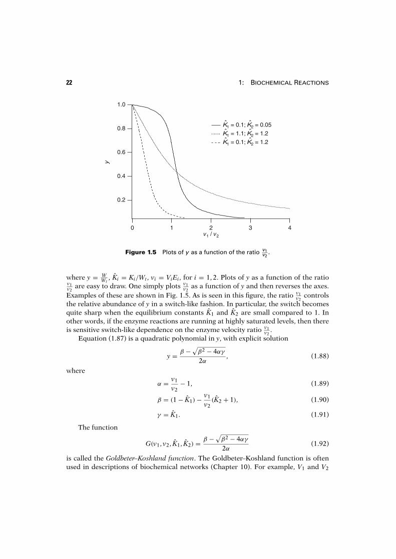
ˆ ˆˆ ˆˆ ˆ
Figure 1.5 Plots of y as a function of the ratio v1v2
.
where y = WWt
, Ki = Ki/Wt, vi = ViEi, for i = 1, 2. Plots of y as a function of the ratiov1v2
are easy to draw. One simply plots v1v2
as a function of y and then reverses the axes.Examples of these are shown in Fig. 1.5. As is seen in this figure, the ratio v1
v2controls
the relative abundance of y in a switch-like fashion. In particular, the switch becomesquite sharp when the equilibrium constants K1 and K2 are small compared to 1. Inother words, if the enzyme reactions are running at highly saturated levels, then thereis sensitive switch-like dependence on the enzyme velocity ratio v1
v2.
Equation (1.87) is a quadratic polynomial in y, with explicit solution
y = β −√β2 − 4αγ2α
, (1.88)
where
α = v1
v2− 1, (1.89)
β = (1− K1)− v1
v2(K2 + 1), (1.90)
γ = K1. (1.91)
The function
G(v1, v2, K1, K2) = β −√β2 − 4αγ2α
(1.92)
is called the Goldbeter–Koshland function. The Goldbeter–Koshland function is oftenused in descriptions of biochemical networks (Chapter 10). For example, V1 and V2
1.5: Glycolysis and Glycolytic Oscillations 23
could depend on the concentration of another enzyme, E say, leading to switch-likeregulation of the concentration of W as a function of the concentration of E. In thisway, networks of biochemical reactions can be constructed in which some of thecomponents are switched on or switched off, relatively abruptly, by other components.
1.5 Glycolysis and Glycolytic Oscillations
Metabolism is the process of extracting useful energy from chemical bonds. A metabolicpathway is the sequence of enzymatic reactions that take place in order to transferchemical energy from one form to another. The common carrier of energy in the cellis the chemical adenosine triphosphate (ATP). ATP is formed by the addition of aninorganic phosphate group (HPO2−
4 ) to adenosine diphosphate (ADP), or by the ad-dition of two inorganic phosphate groups to adenosine monophosphate (AMP). Theprocess of adding an inorganic phosphate group to a molecule is called phosphorylation.Since the three phosphate groups on ATP carry negative charges, considerable energyis required to overcome the natural repulsion of like-charged phosphates as additionalgroups are added to AMP. Thus, the hydrolysis (the cleavage of a bond by water) of ATPto ADP releases large amounts of energy.
Energy to perform chemical work is made available to the cell by the oxidation ofglucose to carbon dioxide and water, with a net release of energy. The overall chemicalreaction for the oxidation of glucose can be written as
C6H12O6 + 6O2 −→ 6CO2 + 6H2O+ energy, (1.93)
but of course, this is not an elementary reaction. Instead, this reaction takes place ina series of enzymatic reactions, with three major reaction stages, glycolysis, the Krebscycle, and the electron transport (or cytochrome) system.
The oxidation of glucose is associated with a large negative free energy, �G0 =−2878.41 kJ/mol, some of which is dissipated as heat. However, in living cells much ofthis free energy in stored in ATP, with one molecule of glucose resulting in 38 moleculesof ATP.
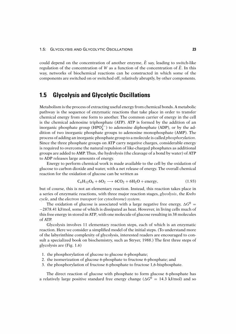
Glycolysis involves 11 elementary reaction steps, each of which is an enzymaticreaction. Here we consider a simplified model of the initial steps. (To understand moreof the labyrinthine complexity of glycolysis, interested readers are encouraged to con-sult a specialized book on biochemistry, such as Stryer, 1988.) The first three steps ofglycolysis are (Fig. 1.6)
1. the phosphorylation of glucose to glucose 6-phosphate;2. the isomerization of glucose 6-phosphate to fructose 6-phosphate; and3. the phosphorylation of fructose 6-phosphate to fructose 1,6-bisphosphate.
The direct reaction of glucose with phosphate to form glucose 6-phosphate hasa relatively large positive standard free energy change (�G0 = 14.3 kJ/mol) and so
24 1: Biochemical Reactions
Glucose
Fructose 6-P
Fructose 1,6-bisP
Glucose 6-P
ATP
ADP
isomerization
PFK1
ATP
ADPFigure 1.6 The first three reactions in the glycolyticpathway.
does not occur significantly under physiological conditions. However, the first stepof metabolism is coupled with the hydrolysis of ATP to ADP (catalyzed by the enzymehexokinase), giving this step a net negative standard free energy change and making thereaction strongly spontaneous. This feature turns out to be important for the efficientoperation of glucose membrane transporters, which are described in the next chapter.
The second step of glycolysis has a relatively small positive standard free energychange (�G0 = 1.7 kJ/mol), with an equilibrium constant of 0.5. This means thatsignificant amounts of product are formed under normal conditions.
The third step is, like the first step, energetically unfavorable, were it not cou-pled with the hydrolysis of ATP. However, the net standard free energy change(�G0 = −14.2 kJ/mol) means that not only is this reaction strongly favored, but alsothat it augments the reaction in the second step by depleting the product of the secondstep.
This third reaction is catalyzed by the enzyme phosphofructokinase (PFK1). PFK1is an example of an allosteric enzyme as it is allosterically inhibited by ATP. Note thatATP is both a substrate of PFK1, binding at a catalytic site, and an allosteric inhibitor,binding at a regulatory site. The inhibition due to ATP is removed by AMP, and thus theactivity of PFK1 increases as the ratio of ATP to AMP decreases. This feedback enablesPFK1 to regulate the rate of glycolysis based on the availability of ATP. If ATP levelsfall, PFK1 activity increases thereby increasing the rate of production of ATP, whereas,if ATP levels become high, PFK1 activity drops shutting down the production of ATP.
1.5: Glycolysis and Glycolytic Oscillations 25
As PFK1 phosphorylates fructose 6-P, ATP is converted to ADP. ADP, in turn, isconverted back to ATP and AMP by the reaction
2ADP −→←− ATP+ AMP,
which is catalyzed by the enzyme adenylate kinase. Since there is normally little AMPin cells, the conversion of ADP to ATP and AMP serves to significantly decrease theATP/AMP ratio, thus activating PFK1. This is an example of a positive feedback loop;the greater the activity of PFK1, the lower the ATP/AMP ratio, thus further increasingPFK1 activity.
It was discovered in 1980 that in some cell types, another important allostericactivator of PFK1 is fructose 2,6-bisphosphate (Stryer, 1988), which is formed fromfructose 6-phosphate in a reaction catalyzed by phosphofructokinase 2 (PFK2), a differ-ent enzyme from phosphofructokinase (PFK1) (you were given fair warning about thelabyrinthine nature of this process!). Of particular significance is that an abundance offructose 6-phosphate leads to a corresponding abundance of fructose 2,6-bisphosphate,and thus a corresponding increase in the activity of PFK1. This is an example of anegative feedback loop, where an increase in the substrate concentration leads to agreater rate of substrate reaction and consumption. Clearly, PFK1 activity is controlledby an intricate system of reactions, the collective behavior of which is not obvious apriori.
Under certain conditions the rate of glycolysis is known to be oscillatory, or evenchaotic (Nielsen et al., 1997). This biochemical oscillator has been known and studiedexperimentally for some time. For example, Hess and Boiteux (1973) devised a flowreactor containing yeast cells into which a controlled amount of substrate (either glu-cose or fructose) was continuously added. They measured the pH and fluorescenceof the reactants, thereby monitoring the glycolytic activity, and they found ranges ofcontinuous input under which glycolysis was periodic.
Interestingly, the oscillatory behavior is different in intact yeast cells and in yeastextracts. In intact cells the oscillations are sinusoidal in shape, and there is strongevidence that they occur close to a Hopf bifurcation (Danø et al., 1999). In yeast extractthe oscillations are of relaxation type, with widely differing time scales (Madsen et al.,2005).
Feedback on PFK is one, but not the only, mechanism that has been proposed ascausing glycolytic oscillations. For example, hexose transport kinetics and autocatal-ysis of ATP have both been proposed as possible mechanisms (Madsen et al., 2005),while some authors have claimed that the oscillations arise as part of the entire net-work of reactions, with no single feedback being of paramount importance (Bier et al.,1996; Reijenga et al., 2002). Here we focus only on PFK regulation as the oscillatorymechanism.
A mathematical model describing glycolytic oscillations was proposed by Sel’kov(1968) and later modified by Goldbeter and Lefever (1972). It is designed to capture onlythe positive feedback of ADP on PFK1 activity. In the Sel’kov model, PFK1 is inactive
26 1: Biochemical Reactions
in its unbound state but is activated by binding with several ADP molecules. Note that,for simplicity, the model does not take into account the conversion of ADP to AMP andATP, but assumes that ADP activates PFK1 directly, since the overall effect is similar.In the active state, the enzyme catalyzes the production of ADP from ATP as fructose-6-P is phosphorylated. Sel’kov’s reaction scheme for this process is as follows: PFK1(denoted by E) is activated or deactivated by binding or unbinding with γ moleculesof ADP (denoted by S2)
γS2 + Ek3−→←−
k−3
ESγ2 ,
and ATP (denoted S1) can bind with the activated form of enzyme to produce a productmolecule of ADP. In addition, there is assumed to be a steady supply rate of S1, whileproduct S2 is irreversibly removed. Thus,
v1−→S1, (1.94)
S1 + ESγ2
k1−→←−k−1
S1ESγ2k2−→ESγ2 + S2, (1.95)
S2v2−→. (1.96)
Note that (1.95) is an enzymatic reaction of exactly Michaelis–Menten form so weshould expect a similar reduction of the governing equations.
Applying the law of mass action to the Sel’kov kinetic scheme, we find five differ-ential equations for the production of the five species s1 = [S1], s2 = [S2], e = [E], x1 =[ESγ2 ], x2 = [S1ESγ2 ]:
ds1
dt= v1 − k1s1x1 + k−1x2, (1.97)
ds2
dt= k2x2 − γk3sγ2 e+ γk−3x1 − v2s2, (1.98)
dx1
dt= −k1s1x1 + (k−1 + k2)x2 + k3sγ2 e− k−3x1, (1.99)
dx2
dt= k1s1x1 − (k−1 + k2)x2. (1.100)
The fifth differential equation is not necessary, because the total available enzyme isconserved, e+x1+x2 = e0. Now we introduce dimensionless variables σ1 = k1s1
k2+k−1, σ2 =
(k3
k−3)1/γ s2, u1 = x1/e0, u2 = x2/e0, t = k2+k−1
e0k1k2τ and find
dσ1
dτ= ν − k2 + k−1
k2u1σ1 + k−1
k2u2, (1.101)
dσ2
dτ= α
[u2 − γk−3
k2σγ
2 (1− u1 − u2)+ γk−3
k2u1
]− ησ2, (1.102)
1.5: Glycolysis and Glycolytic Oscillations 27
εdu1
dτ= u2 − σ1u1 + k−3
k2 + k−1
[σγ
2 (1− u1 − u2)− u1]
, (1.103)
εdu2
dτ= σ1u1 − u2, (1.104)
where ε = e0k1k2(k2+k−1)
2 , ν = v1k2e0
, η = v2(k2+k−1)
k1k2e0,α = k2+k−1
k1(
k3k−3)1/γ . If we assume that ε is a
small number, then both u1 and u2 are fast variables and can be set to their quasi-steadyvalues,
u1 = σγ
2
σγ
2 σ1 + σγ2 + 1, (1.105)
u2 = σ1σγ
2
σγ
2 σ1 + σγ2 + 1= f (σ1, σ2), (1.106)
and with these quasi-steady values, the evolution of σ1 and σ2 is governed by
dσ1
dτ= ν − f (σ1, σ2), (1.107)
dσ2
dτ= αf (σ1, σ2)− ησ2. (1.108)
The goal of the following analysis is to demonstrate that this system of equationshas oscillatory solutions for some range of the supply rate ν. First observe that becauseof saturation, the function f (σ1, σ2) is bounded by 1. Thus, if ν > 1, the solutions of thedifferential equations are not bounded. For this reason we consider only 0 < ν < 1.The nullclines of the flow are given by the equations
σ1 = ν
1− ν1+ σγ2σγ
2
(dσ1
dτ= 0
), (1.109)
σ1 = 1+ σγ2σγ−12 (p− σ2)
(dσ2
dτ= 0
), (1.110)
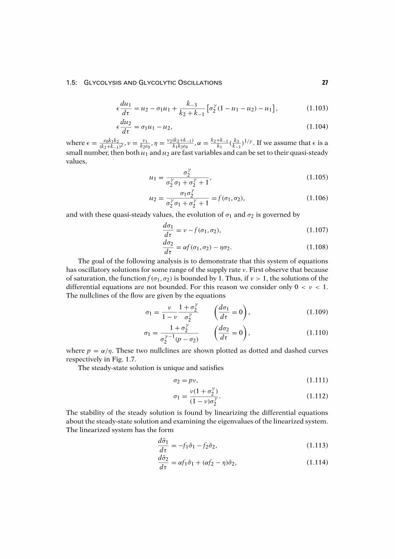
where p = α/η. These two nullclines are shown plotted as dotted and dashed curvesrespectively in Fig. 1.7.
The steady-state solution is unique and satisfies
σ2 = pν, (1.111)
σ1 = ν(1+ σγ2 )(1− ν)σ γ2
. (1.112)
The stability of the steady solution is found by linearizing the differential equationsabout the steady-state solution and examining the eigenvalues of the linearized system.The linearized system has the form
dσ1
dτ= −f1σ1 − f2σ2, (1.113)
dσ2
dτ= αf1σ1 + (αf2 − η)σ2, (1.114)
28 1: Biochemical Reactions
1.0
0.8
0.6
0.4
0.2
0.0
s 2
1.41.21.00.80.60.40.20.0s1
Figure 1.7 Phase portrait of the Sel’kov glycolysis model with ν = 0.0285, η = 0.1,α = 1.0,and γ = 2. Dotted curve: dσ1
dτ = 0. Dashed curve: dσ2dτ = 0.
where fj = ∂f∂σj
, j = 1, 2, evaluated at the steady-state solution, and where σi denotes
the deviation from the steady-state value of σi. The characteristic equation for theeigenvalues λ of the linear system (1.113)–(1.114) is
λ2 − (αf2 − η − f1)λ+ f1η = 0. (1.115)
Since f1 is always positive, the stability of the linear system is determined by the sign ofH = αf2−η− f1, being stable if H < 0 and unstable if H > 0. Changes of stability, if theyexist, occur at H = 0, and are Hopf bifurcations to periodic solutions with approximatefrequency ω = √f1η.
The function H(ν) is given by
H(ν) = (1− ν)(1+ y)
(ηγ + (ν − 1)y)− η, (1.116)
y = (pν)γ . (1.117)
Clearly, H(0) = η(γ − 1), H(1) = −η, so for γ > 1, there must be at least one Hopfbifurcation point, below which the steady solution is unstable. Additional computa-tions show that this Hopf bifurcation is supercritical, so that for ν slightly below thebifurcation point, there is a stable periodic orbit.
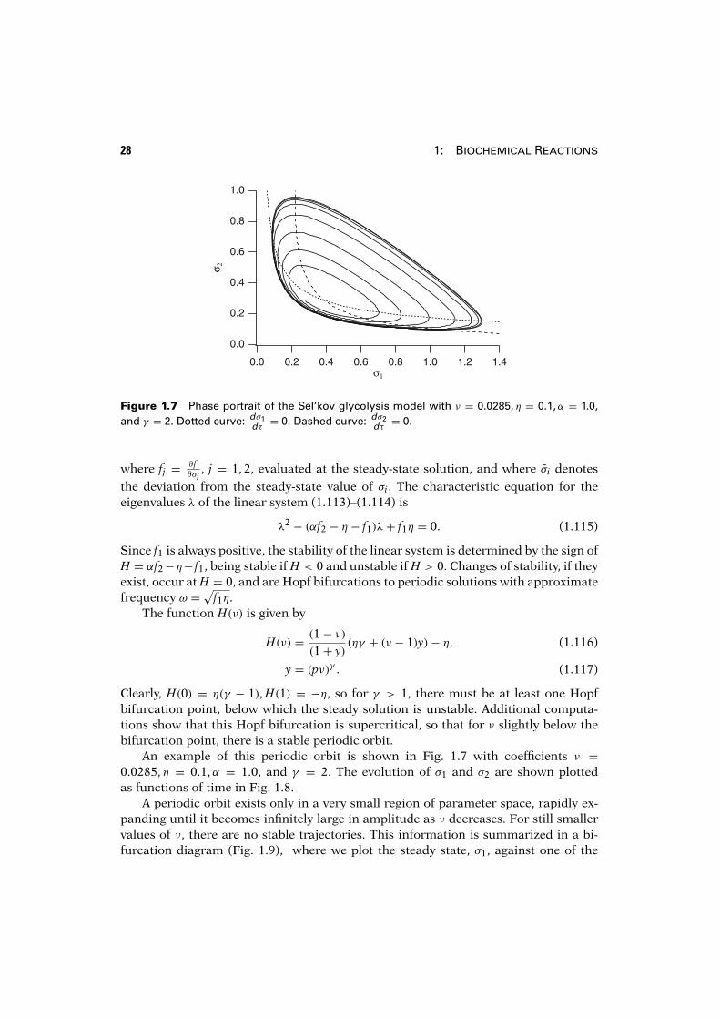
An example of this periodic orbit is shown in Fig. 1.7 with coefficients ν =0.0285, η = 0.1,α = 1.0, and γ = 2. The evolution of σ1 and σ2 are shown plottedas functions of time in Fig. 1.8.
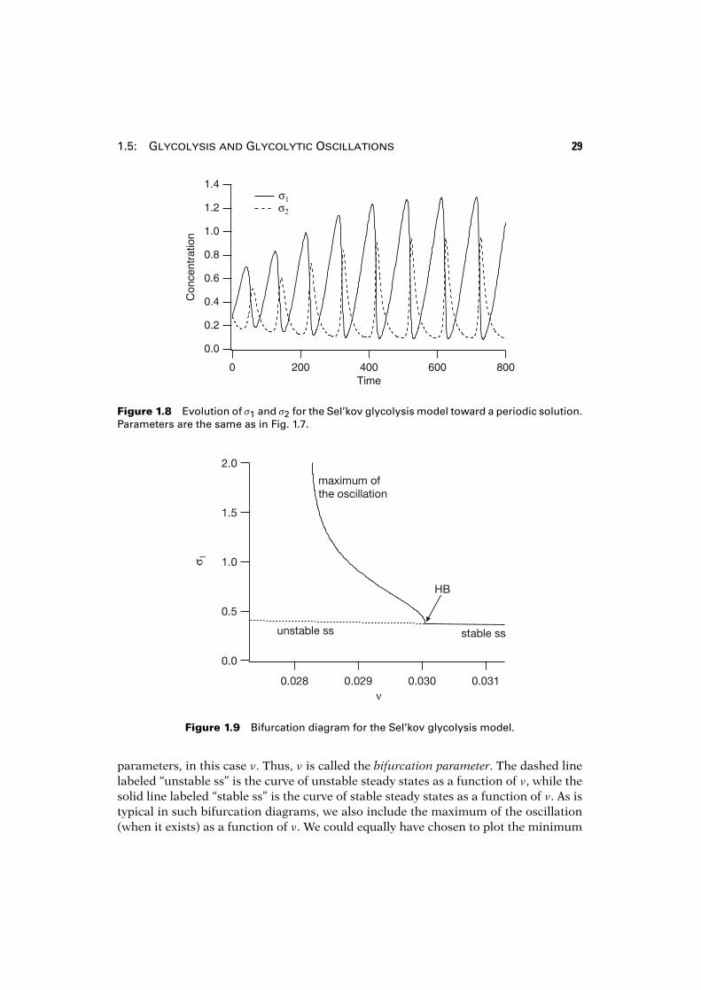
A periodic orbit exists only in a very small region of parameter space, rapidly ex-panding until it becomes infinitely large in amplitude as ν decreases. For still smallervalues of ν, there are no stable trajectories. This information is summarized in a bi-furcation diagram (Fig. 1.9), where we plot the steady state, σ1, against one of the
1.5: Glycolysis and Glycolytic Oscillations 29
1.4
1.2
1.0
0.8
0.6
0.4
0.2
0.0
Con
cent
ratio
n
8006004002000Time
s1s2
Figure 1.8 Evolution of σ1 and σ2 for the Sel’kov glycolysis model toward a periodic solution.Parameters are the same as in Fig. 1.7.
s 1
n
Figure 1.9 Bifurcation diagram for the Sel’kov glycolysis model.
parameters, in this case ν. Thus, ν is called the bifurcation parameter. The dashed linelabeled “unstable ss” is the curve of unstable steady states as a function of ν, while thesolid line labeled “stable ss” is the curve of stable steady states as a function of ν. As istypical in such bifurcation diagrams, we also include the maximum of the oscillation(when it exists) as a function of ν. We could equally have chosen to plot the minimum

30 1: Biochemical Reactions
of the oscillation (or both the maximum and the minimum). Since the oscillation isstable, the maximum of the oscillation is plotted with a solid line.
From the bifurcation diagram we see that the stable branch of oscillations origi-nates at a supercritical Hopf bifurcation (labeled HB), and that the periodic orbits onlyexist for a narrow range of values of ν. The question of how this branch of periodicorbits terminates is not important for the discussion here, so we ignore this importantpoint for now.
We use bifurcation diagrams throughout this book, and many are considerablymore complicated than that shown in Fig. 1.9. Readers who are unfamiliar with the ba-sic theory of nonlinear bifurcations, and their representation in bifurcation diagrams,are urged to consult an elementary book such as Strogatz (1994).
While the Sel’kov model has certain features that are qualitatively correct, it failsto agree with the experimental results at a number of points. Hess and Boiteux (1973)report that for high and low substrate injection rates, there is a stable steady-statesolution. There are two Hopf bifurcation points, one at the flow rate of 20 mM/hrand another at 160 mM/hr. The period of oscillation at the low flow rate is about 8minutes and decreases as a function of flow rate to about 3 minutes at the upperHopf bifurcation point. In contrast, the Sel’kov model has but one Hopf bifurcationpoint.
To reproduce these additional experimental features we consider a more de-tailed model of the reaction. In 1972, Goldbeter and Lefever proposed a model ofMonod–Wyman–Changeux type that provided a more accurate description of the os-cillations. More recently, by fitting a simpler model to experimental data on PFK1kinetics in skeletal muscle, Smolen (1995) has shown that this level of complexity isnot necessary; his model assumes that PFK1 consists of four independent, identicalsubunits, and reproduces the observed oscillations well. Despite this, we describe onlythe Goldbeter–Lefever model in detail, as it provides an excellent example of the use ofMonod–Wyman–Changeux models.
In the Goldbeter–Lefever model of the phosphorylation of fructose-6-P, the enzymePFK1 is assumed to be a dimer that exists in two states, an active state R and aninactive state T. The substrate, S1, can bind to both forms, but the product, S2, whichis an activator, or positive effector, of the enzyme, binds only to the active form. Theenzymatic forms of R carrying substrate decompose irreversibly to yield the productADP. In addition, substrate is supplied to the system at a constant rate, while productis removed at a rate proportional to its concentration. The reaction scheme for this isas follows: let Tj represent the inactive T form of the enzyme bound to j molecules ofsubstrate and let Rij represent the active form R of the enzyme bound to i substratemolecules and j product molecules. This gives the reaction diagram shown in Fig. 1.10.In this system, the substrate S1 holds the enzyme in the inactive state by binding withT0 to produce T1 and T2, while product S2 holds the enzyme in the active state bybinding with R00 to produce R01 and binding with R01 to produce R02. There is a factorof two in the rates of reaction because a dimer with two available binding sites reactslike twice the same amount of monomer.
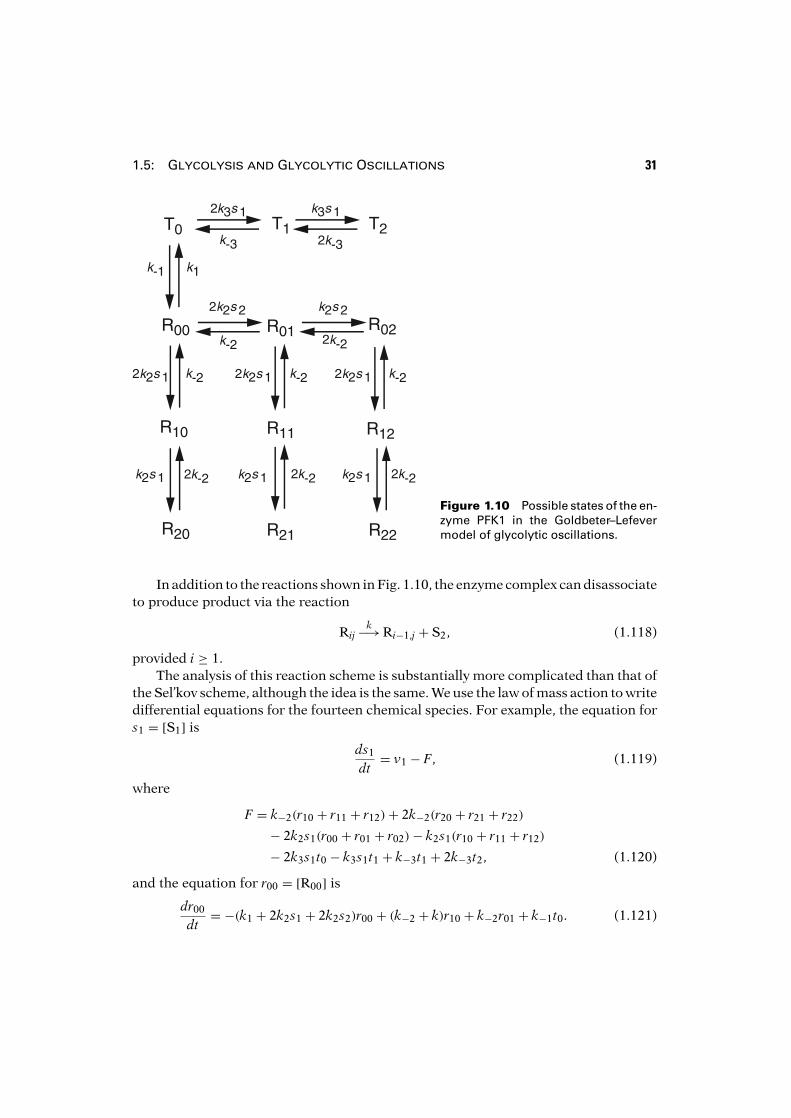
1.5: Glycolysis and Glycolytic Oscillations 31
T0 T1 T2
R00 R01 R02
R10 R11 R12
R20 R21 R22
2k2s 2 k2s 2
k-2 k-2
k-2 k-2 k-2
k-2k-2k-2
2k2s 1 2k2s 1 2k2s 1
k2s 1 k2s 1 k2s 1
k1k-1
k3s 1 k3s 1
k-3 k-3
2
2
2
2 2 2
Figure 1.10 Possible states of the en-zyme PFK1 in the Goldbeter–Lefevermodel of glycolytic oscillations.
In addition to the reactions shown in Fig. 1.10, the enzyme complex can disassociateto produce product via the reaction
Rijk−→Ri−1,j + S2, (1.118)
provided i ≥ 1.The analysis of this reaction scheme is substantially more complicated than that of
the Sel’kov scheme, although the idea is the same. We use the law of mass action to writedifferential equations for the fourteen chemical species. For example, the equation fors1 = [S1] is
ds1
dt= v1 − F, (1.119)
where
F = k−2(r10 + r11 + r12)+ 2k−2(r20 + r21 + r22)
− 2k2s1(r00 + r01 + r02)− k2s1(r10 + r11 + r12)
− 2k3s1t0 − k3s1t1 + k−3t1 + 2k−3t2, (1.120)
and the equation for r00 = [R00] isdr00
dt= −(k1 + 2k2s1 + 2k2s2)r00 + (k−2 + k)r10 + k−2r01 + k−1t0. (1.121)
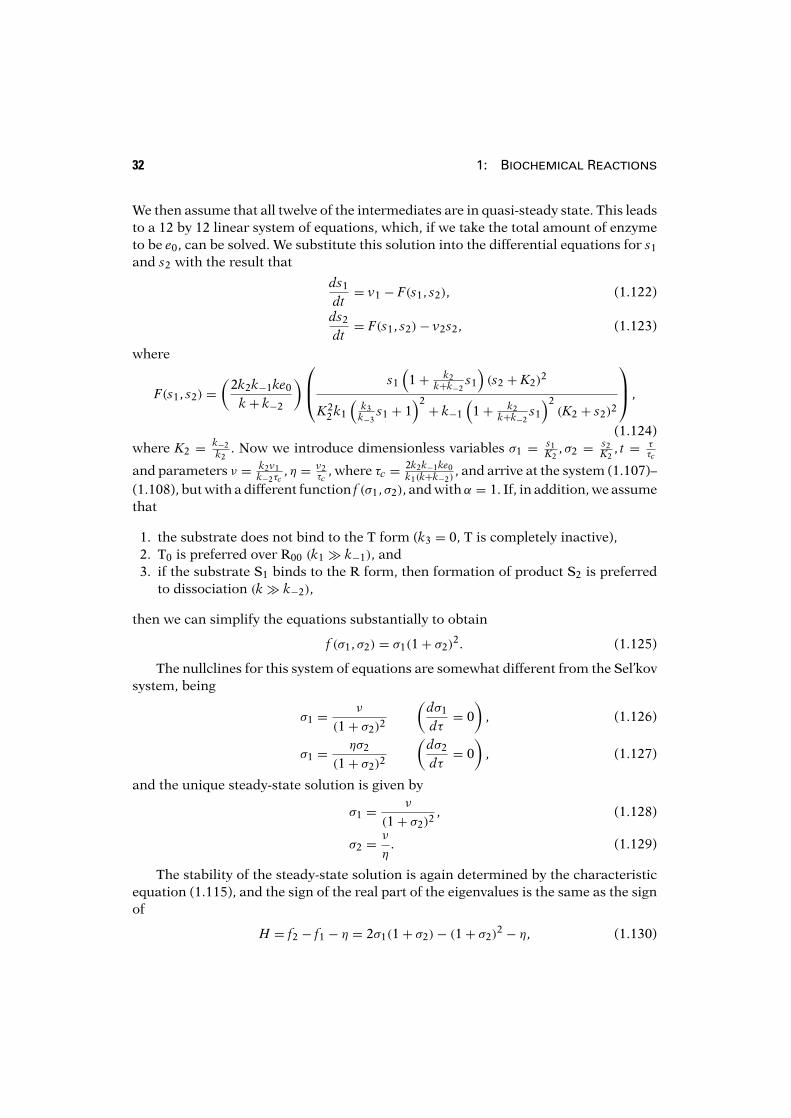
32 1: Biochemical Reactions
We then assume that all twelve of the intermediates are in quasi-steady state. This leadsto a 12 by 12 linear system of equations, which, if we take the total amount of enzymeto be e0, can be solved. We substitute this solution into the differential equations for s1
and s2 with the result that
ds1
dt= v1 − F(s1, s2), (1.122)
ds2
dt= F(s1, s2)− v2s2, (1.123)
where
F(s1, s2) =(
2k2k−1ke0
k+ k−2
)⎛
⎜⎝s1
(1+ k2
k+k−2s1
)(s2 + K2)
2
K22 k1
(k3
k−3s1 + 1
)2 + k−1
(1+ k2
k+k−2s1
)2(K2 + s2)
2
⎞
⎟⎠ ,
(1.124)where K2 = k−2
k2. Now we introduce dimensionless variables σ1 = s1
K2, σ2 = s2
K2, t = τ
τc
and parameters ν = k2v1k−2τc
, η = v2τc
, where τc = 2k2k−1ke0k1(k+k−2)
, and arrive at the system (1.107)–(1.108), but with a different function f (σ1, σ2), and with α = 1. If, in addition, we assumethat
1. the substrate does not bind to the T form (k3 = 0, T is completely inactive),2. T0 is preferred over R00 (k1 � k−1), and3. if the substrate S1 binds to the R form, then formation of product S2 is preferred
to dissociation (k� k−2),
then we can simplify the equations substantially to obtain
f (σ1, σ2) = σ1(1+ σ2)2. (1.125)
The nullclines for this system of equations are somewhat different from the Sel’kovsystem, being
σ1 = ν
(1+ σ2)2
(dσ1
dτ= 0
), (1.126)
σ1 = ησ2
(1+ σ2)2
(dσ2
dτ= 0
), (1.127)
and the unique steady-state solution is given by
σ1 = ν
(1+ σ2)2 , (1.128)
σ2 = ν
η. (1.129)
The stability of the steady-state solution is again determined by the characteristicequation (1.115), and the sign of the real part of the eigenvalues is the same as the signof
H = f2 − f1 − η = 2σ1(1+ σ2)− (1+ σ2)2 − η, (1.130)
1.6: Appendix: Math Background 33
evaluated at the steady state (1.126)–(1.127). Equation (1.130) can be written as thecubic polynomial
1η
y3 − y+ 2 = 0, y = 1+ νη
. (1.131)
For η sufficiently large, the polynomial (1.131) has two roots greater than 2, say, y1 andy2. Recall that ν is the nondimensional flow rate of substrate ATP. To make some corre-spondence with the experimental data, we assume that the flow rate ν is proportionalto the experimental supply rate of glucose. This is not strictly correct, although ATP isproduced at about the same rate that glucose is supplied. Accepting this caveat, we seethat to match experimental data, we require
y2 − 1y1 − 1
= ν2
ν1= 160
20= 8. (1.132)
Requiring (1.131) to hold at y1 and y2 and requiring (1.132) to hold as well, we findnumerical values
y1 = 2.08, y2 = 9.61, η = 116.7, (1.133)
corresponding to ν1 = 126 and ν2 = 1005.At the Hopf bifurcation point, the period of oscillation is
Ti = 2πωi= 2π√
η(1+ σ2)= 2π√
ηyi. (1.134)
For the numbers (1.133), we obtain a ratio of periods T1/T2 = 4.6, which is acceptablyclose to the experimentally observed ratio T1/T2 = 2.7.
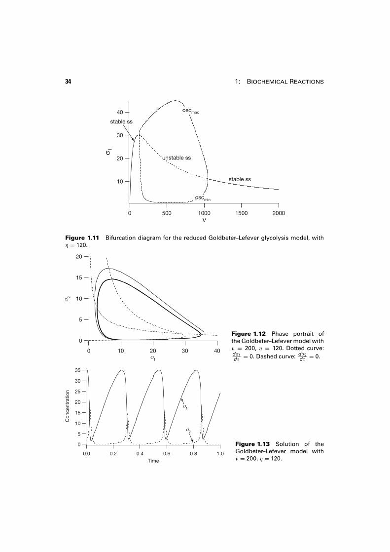
The behavior of the solution as a function of the parameter ν is summarized inthe bifurcation diagram, Fig. 1.11, shown here for η = 120. The steady-state solutionis stable below η = 129 and above η = 1052. Between these values of η the steady-state solution is unstable, but there is a branch of stable periodic solutions whichterminates and collapses into the steady-state solution at the two points where thestability changes, the Hopf bifurcation points.
A typical phase portrait for the periodic solution that exists between the Hopfbifurcation points is shown in Fig. 1.12, and the concentrations of the two speciesare shown as functions of time in Fig. 1.13.
1.6 Appendix: Math Background
It is certain that some of the mathematical concepts and tools that we routinely in-voke here are not familiar to all of our readers. In this first chapter alone, we haveused nondimensionalization, phase-plane analysis, linear stability analysis, bifurca-tion theory, and asymptotic analysis, all the while assuming that these are familiar tothe reader.
34 1: Biochemical Reactions
s 1
n
Figure 1.11 Bifurcation diagram for the reduced Goldbeter–Lefever glycolysis model, withη = 120.
Figure 1.12 Phase portrait ofthe Goldbeter–Lefever model withν = 200, η = 120. Dotted curve:dσ1dτ = 0. Dashed curve: dσ2
dτ = 0.
Figure 1.13 Solution of theGoldbeter–Lefever model withν = 200, η = 120.
1.6: Appendix: Math Background 35
The purpose of this appendix is to give a brief guide to those techniques that are abasic part of the applied mathematician’s toolbox.
1.6.1 Basic Techniques
In any problem, there are a number of parameters that are dictated by the problem.However, it often happens that not all parameter variations are independent; that is,different variations in different parameters may lead to identical changes in the behav-ior of the model. Second, there may be parameters whose influence on a behavior isnegligible and can be safely ignored for a given context.
The way to identify independent parameters and to determine their relative mag-nitudes is to nondimensionalize the problem. Unfortunately, there is not a uniquealgorithm for nondimensionalization; nondimensionalization is as much art as it isscience.
There are, however, rules of thumb to apply. In any system of equations, thereare a number of independent variables (time, space, etc.), dependent variables(concentrations, etc.) and parameters (rates of reaction, sizes of containers, etc.).Nondimensionalization begins by rescaling the independent and dependent variablesby “typical” units, rendering them thereby dimensionless. One goal may be to ensurethat the dimensionless variables remain of a fixed order of magnitude, not becomingtoo large or negligibly small. This usually requires some a priori knowledge about thesolution, as it can be difficult to choose typical scales unless something is already knownabout typical solutions. Time and space scales can be vastly different depending on thecontext.
Once this selection of scales has been made, the governing equations are writtenin terms of the rescaled variables and dimensionless combinations of the remainingparameters are identified. The number of remaining free dimensionless parameters isusually less than the original number of physical parameters. The primary difficulty(at least to understand and apply the process) is that there is not necessarily a singleway to scale and nondimensionalize the equations. Some scalings may highlight cer-tain features of the solution, while other scalings may emphasize others. Nonetheless,nondimensionalization often (but not always) provides a good starting point for theanalysis of a model system.
An excellent discussion of scaling and nondimensionalization can be found in Linand Segel (1988, Chapter 6). A great deal of more advanced work has also been doneon this subject, particularly its application to the quasi-steady-state approximation, bySegel and his collaborators (Segel, 1988; Segel and Slemrod, 1989; Segel and Perelson,1992; Segel and Goldbeter, 1994; Borghans et al., 1996; see also Frenzen and Maini,1988).
Phase-plane analysis and linear stability analysis are standard fare in introductorycourses on differential equations. A nice introduction to these topics for the biologicallyinclined can be found in Edelstein-Keshet (1988, Chapter 5) or Braun (1993, Chapter4). A large number of books discuss the qualitative theory of differential equations,

36 1: Biochemical Reactions
for example, Boyce and Diprima (1997), or at a more advanced level, Hale and Koçak(1991), or Hirsch and Smale (1974).
Bifurcation TheoryBifurcation theory is a topic that is gradually finding its way into introductory litera-ture. The most important terms to understand are those of steady-state bifurcations,Hopf bifurcations, homoclinic bifurcations, and saddle-node bifurcations, all of whichappear in this book. An excellent introduction to these concepts is found in Strogatz(1994, Chapters 3, 6, 7, 8), and an elementary treatment, with particular application tobiological systems, is given by Beuter et al. (2003, Chapters 2, 3). More advanced treat-ments include those in Guckenheimer and Holmes (1983), Arnold (1983) or Wiggins(2003).
One way to summarize the behavior of the model is with a bifurcation diagram(examples of which are shown in Figs. 1.9 and 1.11), which shows how certain featuresof the model, such as steady states or limit cycles, vary as a parameter is varied. Whenmodels have many parameters there is a wide choice for which parameter to vary. Often,however, there are compelling physiological or experimental reasons for the choice ofparameter. Bifurcation diagrams are important in a number of chapters of this book,and are widely used in the analysis of nonlinear systems. Thus, it is worth the timeto become familiar with their properties and how they are constructed. Nowadays,most bifurcation diagrams of realistic models are constructed numerically, the mostpopular choice of software being AUTO (Doedel, 1986; Doedel et al., 1997, 2001). Thebifurcation diagrams in this book were all prepared with XPPAUT (Ermentrout, 2002),a convenient implementation of AUTO.
In this text, the bifurcation that is seen most often is the Hopf bifurcation. TheHopf bifurcation theorem describes conditions for the appearance of small periodicsolutions of a differential equation, say
dudt= f (u, λ), (1.135)
as a function of the parameter λ. Suppose that there is a steady-state solution, u = u0(λ),and that the system linearized about u0,
dUdt= ∂f (u0(λ), λ)
∂uU, (1.136)
has a pair of complex eigenvalues μ(λ) = α(λ)± iβ(λ). Suppose further that α(λ0) = 0,α′(λ0) �= 0, and β(λ0) �= 0, and that at λ = λ0 no other eigenvalues of the system havezero real part. Then λ0 is a Hopf bifurcation point, and there is a branch of periodicsolutions emanating from the point λ = λ0. The periodic solutions could exist (locally)for λ > λ0, for λ < λ0, or in the degenerate (nongeneric) case, for λ = λ0. If the periodicsolutions occur in the region of λ for which α(λ) > 0, then the periodic solutionsare stable (provided all other eigenvalues of the system have negative real part), andthis branch of solutions is said to be supercritical. On the other hand, if the periodic
1.6: Appendix: Math Background 37
solutions occur in the region of λ for which α(λ) < 0, then the periodic solutions areunstable, and this branch of solutions is said to be subcritical.
The Hopf bifurcation theorem applies to ordinary differential equations and delaydifferential equations. For partial differential equations, there are some technical issueshaving to do with the nature of the spectrum of the linearized operator that complicatematters, but we do not concern ourselves with these here. Instead, rather than checkingall the conditions of the theorem, we find periodic solutions by looking only for a changeof the sign of the real part of an eigenvalue, using numerical computations to verifythe existence of periodic solutions, and calling it good.
1.6.2 Asymptotic Analysis
Applied mathematicians love small parameters, because of the hope that the solutionof a problem with a small parameter might be approximated by an asymptotic represen-tation. A commonplace notation has emerged in which ε is often the small parameter.An asymptotic representation has a precise mathematical meaning. Suppose that G(ε)is claimed to be an asymptotic representation of g(ε), expressed as
g(ε) = G(ε)+O(φ(ε)). (1.137)
The precise meaning of this statement is that there is a constant A such that∣∣∣∣g(ε)−G(ε)
φ(ε)
∣∣∣∣ ≤ A (1.138)
for all ε with |ε| ≤ ε0 and ε > 0. The function φ(ε) is called a gauge function, a typicalexample of which is a power of ε.
Perturbation ExpansionsIt is often the case that an asymptotic representation can be found as a power series inpowers of the small parameter ε. Such representations are called perturbation expan-sions. Usually, a few terms of this power series representation suffice to give a goodapproximation to the solution. It should be kept in mind that under no circumstancesdoes this power series development imply that a complete power series (with an infinitenumber of terms) exists or is convergent. Terminating the series at one or two terms isdeliberate.
However, there are times when a full power series could be found and would beconvergent in some nontrivial ε domain. Such problems are called regular perturbationproblems because their solutions are regular, or analytic, in the parameter ε.
There are numerous examples of regular perturbation problems, including all ofthose related to bifurcation theory. These problems are regular because their solutionscan be developed in a convergent power series of some parameter.
There are, however, many problems with small parameters whose solutions arenot regular, called singular perturbation problems. Singular perturbation problems are
38 1: Biochemical Reactions
characterized by the fact that their dependence on the small parameter is not regular,but singular, and their convergence as a function of ε is not uniform.
Singular problems come in two basic varieties. Characteristic of the first type is asmall region of width ε somewhere in the domain of interest (either space or time) inwhich the solution changes rapidly. For example, the solution of the boundary valueproblem
εu′′ + u′ + u = 0 (1.139)
subject to boundary conditions u(0) = u(1) = 1 is approximated by the asymptoticrepresentation
u(x; ε) = (1− e)e−x/ε + e1−x +O(ε). (1.140)
Notice the nonuniform nature of this solution, as
e = limx→0+
(limε→0+
u(x; ε))�= lim
ε→0+
(lim
x→0+u(x; ε)
)= 1.
Here the term e−x/ε is a boundary layer correction, as it is important only in a smallregion near the boundary at x = 0.
Other terms that are typical in singular perturbation problems are interior layersor transition layers, typified by expressions of the form tan( x−x0
ε), and corner layers,
locations where the derivative changes rapidly but the solution itself changes little.Transition layers are of great significance in the study of excitable systems (Chapter 5).While corner layers show up in this book, we do not study or use them in any detail.
Singular problems of this type can often be identified by the fact that the order ofthe system decreases if ε is set to zero. An example that we have already seen is thequasi-steady-state analysis used to simplify reaction schemes in which some reactionsare significantly faster than others. Setting ε to zero in these examples reduces theorder of the system of equations, signaling a possible problem. Indeed, solutions ofthese equations typically have initial layers near time t = 0. We take a closer look atthis example below.
The second class of singular perturbation problems is that in which there are twoscales in operation everywhere in the domain of interest. Problems of this type showup throughout this book. For example, action potential propagation in cardiac tissueis through a cellular medium whose detailed structure varies rapidly compared to thelength scale of the action potential wave front. Physical properties of the cochlearmembrane in the inner ear vary slowly compared to the wavelength of waves thatpropagate along it. For problems of this type, one must make explicit the dependence onmultiple scales, and so solutions are often expressed as functions of two variables, sayx and x/ε, which are treated as independent variables. Solution techniques that exploitthe multiple-scale nature of the solution are called multiscale methods or averagingmethods.
Detailed discussions of these asymptotic methods may be found in Murray (1984),Kevorkian and Cole (1996), and Holmes (1995).
1.6: Appendix: Math Background 39
1.6.3 Enzyme Kinetics and Singular Perturbation Theory
In most of the examples of enzyme kinetics discussed in this chapter, extensive use wasmade of the quasi-steady-state approximation (1.44), according to which the concen-tration of the complex remains constant during the course of the reaction. Although thisassumption gives the right answers (which, some might argue, is justification enough),mathematicians have sought for ways to justify this approximation rigorously. Bowenet al. (1963) and Heineken et al. (1967) were the first to show that the quasi-steady-stateapproximation can be derived as the lowest-order term in an asymptotic expansion ofthe solution. This has since become one of the standard examples of the applicationof singular perturbation theory to biological systems, and it is discussed in detail byRubinow (1973), Lin and Segel (1988), and Murray (2002), among others.
Starting with (1.37) and (1.38),
dσdτ= −σ + x(σ + α), (1.141)
εdxdτ= σ − x(σ + κ), (1.142)
with initial conditions
σ(0) = 1, (1.143)
x(0) = 0, (1.144)
we begin by looking for solutions of the form
σ = σ0 + εσ1 + ε2σ2 + · · · , (1.145)
x = x0 + εx1 + ε2x2 + · · · . (1.146)
We substitute these solutions into the differential equations and equate coefficientsof powers of ε. To lowest order (i.e., equating all those terms with no ε) we get
dσ0
dτ= −σ0 + x0(σ0 + α), (1.147)
0 = σ0 − x0(σ0 + κ). (1.148)
Note that, because we are matching powers of ε, the differential equation for x hasbeen converted into an algebraic equation for x0, which can be solved to give
x0 = σ0
σ0 + κ . (1.149)
It follows that
dσ0
dτ= −σ0 + x0(σ0 + α) = −σ0
(κ − ασ0 + κ
). (1.150)
These solutions for x0 and σ0 (i.e., for the lowest-order terms in the power seriesexpansion) are the quasi-steady-state approximation of Section 1.4.2. We could carry
40 1: Biochemical Reactions
on and solve for σ1 and x1, but since the calculations rapidly become quite tedious,with little to no benefit, the lowest-order solution suffices.
However, it is important to notice that this lowest-order solution cannot be correctfor all times. For, clearly, the initial conditions σ(0) = 1, x(0) = 0 are inconsistent with(1.149). In fact, by setting ε to be zero, we have decreased the order of the differentialequations system, making it impossible to satisfy the initial conditions.
There must therefore be a brief period of time at the start of the reaction duringwhich the quasi-steady-state approximation does not hold. It is not that ε is not small,but rather that ε dx
dt is not small during this initial period, since dx/dt is large. Indeed, itis during this initial time period that the enzyme is “filling up” with substrate, until theconcentration of complexed enzyme reaches the value given by the quasi-steady-stateapproximation. Since there is little enzyme compared to the total amount of substrate,the concentration of substrate remains essentially constant during this period.
For most biochemical reactions this transition to the quasi-steady state happensso fast that it is not physiologically important, but for mathematical reasons, it isinteresting to understand these kinetics for early times as well. To see how the reactionbehaves for early times, we make a change of time scale, η = τ/ε. This change ofvariables expands the time scale on which we look at the reaction and allows us tostudy events that happen on a fast time scale. To be more precise, we also denote thesolution on this fast time scale by a tilde. In the new time scale, (1.37)–(1.38) become
dσdη= ε(−σ + x(σ + α)), (1.151)
dxdη= σ − x(σ + κ). (1.152)
The initial conditions are σ (0) = 1, x(0) = 0.As before, we expand σ and x in power series in ε, substitute into the differential
equations, and equate coefficients of powers of ε. To lowest order in ε this gives
dσ0
dη= 0, (1.153)
dx0
dη= σ0 − x0(σ0 + κ). (1.154)
Simply stated, this means that σ0 does not change on this time scale, so that σ0 = 1.Furthermore, we can solve for x0 as
x0 = 11+ κ (1− e−(1+κ)η), (1.155)
where we have used the initial condition x0(0) = 0.Once again, we could go on to solve for σ1 and x1, but such calculations, being long
and of little use, are rarely done. Thus, from now on, we omit the subscript 0, since itplays no essential role.
One important thing to notice about this solution for σ and x is that it cannot bevalid at large times. After all, σ cannot possibly be a constant for all times. Thus, σ and
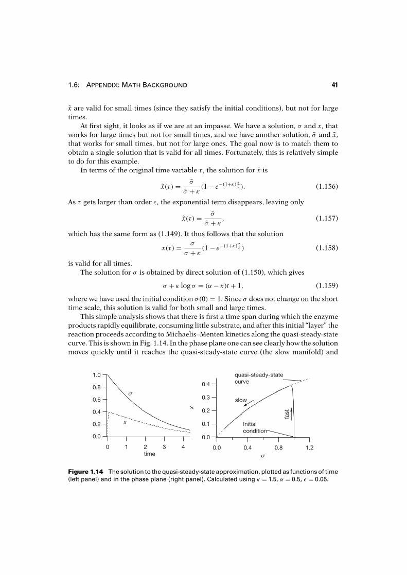
1.6: Appendix: Math Background 41
x are valid for small times (since they satisfy the initial conditions), but not for largetimes.
At first sight, it looks as if we are at an impasse. We have a solution, σ and x, thatworks for large times but not for small times, and we have another solution, σ and x,that works for small times, but not for large ones. The goal now is to match them toobtain a single solution that is valid for all times. Fortunately, this is relatively simpleto do for this example.
In terms of the original time variable τ , the solution for x is
x(τ ) = σ
σ + κ (1− e−(1+κ)τε ). (1.156)
As τ gets larger than order ε, the exponential term disappears, leaving only
x(τ ) = σ
σ + κ , (1.157)
which has the same form as (1.149). It thus follows that the solution
x(τ ) = σ
σ + κ (1− e−(1+κ)τε ) (1.158)
is valid for all times.The solution for σ is obtained by direct solution of (1.150), which gives
σ + κ log σ = (α − κ)t+ 1, (1.159)
where we have used the initial condition σ(0) = 1. Since σ does not change on the shorttime scale, this solution is valid for both small and large times.
This simple analysis shows that there is first a time span during which the enzymeproducts rapidly equilibrate, consuming little substrate, and after this initial “layer” thereaction proceeds according to Michaelis–Menten kinetics along the quasi-steady-statecurve. This is shown in Fig. 1.14. In the phase plane one can see clearly how the solutionmoves quickly until it reaches the quasi-steady-state curve (the slow manifold) and
Figure 1.14 The solution to the quasi-steady-state approximation, plotted as functions of time(left panel) and in the phase plane (right panel). Calculated using κ = 1.5, α = 0.5, ε = 0.05.
42 1: Biochemical Reactions
then moves slowly along that curve toward the steady state. Note that the movementto the quasi-steady-state curve is almost vertical, since during that time σ remainsapproximately unchanged from its initial value. A similar procedure can be followedfor the equilibrium approximation (Exercise 20). In this case, the fast movement tothe slow manifold is not along lines of constant σ , but along lines of constant σ + αx,where α = e0/s0.
In this problem, the analysis of the initial layer is relatively easy and not particularlyrevealing. However, this type of analysis is of much greater importance later in this bookwhen we discuss the behavior of excitable systems.
1.7 Exercises1. Consider the simple chemical reaction in which two monomers of A combine to form a
dimer B, according to
A + Ak+−→←−k−
B.
(a) Use the law of mass action to find the differential equations governing the rates ofproduction of A and B.
(b) What quantity is conserved? Use this conserved quantity to find an equation governingthe rate of production of A that depends only on the concentration of A.
(c) Nondimensionalize this equation and show that these dynamics depend on only onedimensionless parameter.
2. In the real world trimolecular reactions are rare, although trimerizations are not. Considerthe following trimerization reaction in which three monomers of A combine to form thetrimer C,
A + Ak1−→←−
k−1
B,
A + Bk2−→←−
k−2
C.
(a) Use the law of mass action to find the rate of production of the trimer C.
(b) Suppose k−1 � k−2, k2A. Use the appropriate quasi-steady-state approximation tofind the rates of production of A and C, and show that the rate of production of C isproportional to [A]3. Explain in words why this is so.
3. The length of microtubules changes by a process called treadmilling, in which monomer isadded to one end of the microtubule and taken off at the other end. To model this process,suppose that monomer A1 is self-polymerizing in that it can form dimer A2 via
A1 + A1k+−→A2.
1.7: Exercises 43
Furthermore, suppose A1 can polymerize an n-polymer An at one end making an n + 1-polymer An+1
A1 + Ank+−→An+1.
Finally, degradation can occur one monomer at a time from the opposite end at rate k−.Find the steady-state distribution of polymer lengths after an initial amount of monomerA0 has fully polymerized.
4. Suppose that the reaction rates for the three reactant loop of Fig. 1.1 do not satisfy detailedbalance. What is the net rate of conversion of A into B when the reaction is at steady state?
5. Consider an enzymatic reaction in which an enzyme can be activated or inactivated by thesame chemical substance, as follows:
E+Xk1−→←−
k−1
E1, (1.160)
E1 +Xk2−→←−
k−2
E2, (1.161)
E1 + Sk3−→ P+Q+ E. (1.162)
Suppose further that X is supplied at a constant rate and removed at a rate proportionalto its concentration. Use quasi-steady-state analysis to find the nondimensional equationdescribing the degradation of X,
dxdt= γ − x− βxy
1+ x+ y+ αδ x2
. (1.163)
Identify all the parameters and variables, and the conditions under which the quasi-steadystate approximation is valid.
6. Using the quasi-steady-state approximation, show that the velocity of the reaction for anenzyme with an allosteric inhibitor (Section 1.4.3) is given by
V =(
VmaxK3i+ K3
)(s(k−1 + k3i+ k1s+ k−3)
k1(s+ K1)2 + (s+ K1)(k3i+ k−3 + k2)+ k2k−3/k1
). (1.164)
Identify all parameters. Under what conditions on the rate constants is this a validapproximation? Show that this reduces to (1.59) in the case K1 = κ1.
7. (a) Derive the expression (1.76) for the fraction of occupied sites in a Monod–Wyman–Changeux model with n binding sites.
(b) Modify the Monod–Wyman–Changeux model shown in Fig. 1.4 to include transitionsbetween states R1 and T1, and between states R2 and T2. Use the principle of de-tailed balance to derive an expression for the equilibrium constant of each of thesetransitions. Find the expression for Y , the fraction of occupied sites, and compare itto (1.72).
8. An enzyme-substrate system is believed to proceed at a Michaelis–Menten rate. Data forthe (initial) rate of reaction at different concentrations is shown in Table 1.1.
(a) Plot the data V vs. s. Is there evidence that this is a Michaelis–Menten type reaction?
(b) Plot V vs. V/s. Are these data well approximated by a straight line?
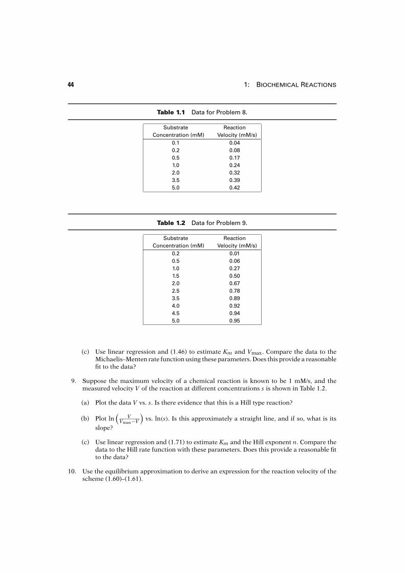
44 1: Biochemical Reactions
.Table 1.1 Data for Problem 8.
Substrate ReactionConcentration (mM) Velocity (mM/s)
0.1 0.040.2 0.080.5 0.171.0 0.242.0 0.323.5 0.395.0 0.42
.Table 1.2 Data for Problem 9.
Substrate ReactionConcentration (mM) Velocity (mM/s)
0.2 0.010.5 0.061.0 0.271.5 0.502.0 0.672.5 0.783.5 0.894.0 0.924.5 0.945.0 0.95
(c) Use linear regression and (1.46) to estimate Km and Vmax. Compare the data to theMichaelis–Menten rate function using these parameters. Does this provide a reasonablefit to the data?
9. Suppose the maximum velocity of a chemical reaction is known to be 1 mM/s, and themeasured velocity V of the reaction at different concentrations s is shown in Table 1.2.
(a) Plot the data V vs. s. Is there evidence that this is a Hill type reaction?
(b) Plot ln(
VVmax−V
)vs. ln(s). Is this approximately a straight line, and if so, what is its
slope?
(c) Use linear regression and (1.71) to estimate Km and the Hill exponent n. Compare thedata to the Hill rate function with these parameters. Does this provide a reasonable fitto the data?
10. Use the equilibrium approximation to derive an expression for the reaction velocity of thescheme (1.60)–(1.61).
1.7: Exercises 45
Answer:
V = (k2K3 + k4s)e0s
K1K3 + K3s+ s2, (1.165)
where K1 = k−1/k1 and K3 = k−3/k3.
11. (a) Find the velocity of reaction for an enzyme with three active sites.
(b) Under what conditions does the velocity reduce to a Hill function with exponent three?Identify all parameters.
(c) What is the relationship between rate constants when the three sites are independent?What is the velocity when the three sites are independent?
12. The Goldbeter–Koshland function (1.92) is defined using the solution of the quadraticequation with a negative square root. Why?
13. Suppose that a substrate can be broken down by two different enzymes with differentkinetics. (This happens, for example, in the case of cAMP or cGMP, which can be hydrolyzedby two different forms of phosphodiesterase—see Chapter 19).
(a) Write the reaction scheme and differential equations, and nondimensionalize, to getthe system of equations
dσdt= −σ + α1(μ1 + σ)x+ α2(μ2 + σ)y, (1.166)
ε1dxdt= 1λ1σ(1− x)− x, (1.167)
ε2dydt= 1λ2σ(1− y)− y. (1.168)
where x and y are the nondimensional concentrations of the two complexes. Identifyall parameters.
(b) Apply the quasi-steady-state approximation to find the equation governing the dy-namics of substrate σ . Under what conditions is the quasi-steady-state approximationvalid?
(c) Solve the differential equation governing σ .
(d) For this system of equations, show that the solution can never leave the positive octantσ , x, y ≥ 0. By showing that σ+ε1x+ε2y is decreasing everywhere in the positive octant,show that the solution approaches the origin for large time.
14. For some enzyme reactions (for example, the hydrolysis of cAMP by phosphodiesterase invertebrate retinal cones) the enzyme is present in large quantities, so that e0/s0 is not a smallnumber. Fortunately, there is an alternate derivation of the Michaelis–Menten rate equationthat does not require that ε = e0
s0be small. Instead, if one or both of k−1 and k2 are much
larger than k1e0, then the formation of complex c is a rapid exponential process, and can betaken to be in quasi-steady state. Make this argument systematic by introducing appropriatenondimensional variables and then find the resulting quasi-steady-state dynamics. (Segel,1988; Frenzen and Maini, 1988; Segel and Slemrod, 1989; Sneyd and Tranchina, 1989).
46 1: Biochemical Reactions
15. ATP is known to inhibit its own dephosphorylation. One possible way for this to occur is ifATP binds with the enzyme, holding it in an inactive state, via
S1 + Ek4−→←−
k−4
S1E.
Add this reaction to the Sel’kov model of glycolysis and derive the equations governingglycolysis of the form (1.107)–(1.108). Explain from the model why this additional reactionis inhibitory.
16. In the case of noncompetitive inhibition, the inhibitor combines with the enzyme-substratecomplex to give an inactive enzyme-substrate-inhibitor complex which cannot undergofurther reaction, but the inhibitor does not combine directly with free enzyme or affect itsreaction with substrate. Use the quasi-steady-state approximation to show that the velocityof this reaction is
V = Vmaxs
Km + s+ iKi
s. (1.169)
Identify all parameters. Compare this velocity with the velocity for other types of inhibitiondiscussed in the text.
17. The following reaction scheme is a simplified version of the Goldbeter–Lefever reactionscheme for glycolytic oscillations:
R0
k1−→←−k−1
T0,
S1 +Rj
k2−→←−k−2
Cjk−→Rj + S2, j = 0, 1, 2,
S2 +R0
2k3−→←−k−3
R1,
S2 +R1
k3−→←−2k−3
R2.
Show that, under appropriate assumptions about the ratios k1/k−1 and k−2+k3k2
the equa-
tions describing this reaction are of the form (1.107)–(1.108) with f (σ1, σ2) given by(1.125).
18. Use the law of mass action and the quasi-steady-state assumption for the enzymatic reac-tions to derive a system of equations of the form (1.107)–(1.108) for the Goldbeter–Lefevermodel of glycolytic oscillations. Verify (1.124).
19. When much of the ATP is depleted in a cell, a considerable amount of cAMP is formed asa product of ATP degradation. This cAMP activates an enzyme phosphorylase that splitsglycogen, releasing glucose that is rapidly metabolized, replenishing the ATP supply.
Devise a model of this control loop and determine conditions under which theproduction of ATP is oscillatory.
20. (a) Nondimensionalize (1.26)–(1.29) in a way appropriate for the equilibrium approxima-tion (rather than the quasi-steady-state approximation of Section 1.4.2). Hint: Recallthat for the equilibrium approximation, the assumption is that k1e0 and k−1 are large
1.7: Exercises 47
compared to k2. You should end up with equations that look something like
εdσdτ= αx− βασ(1− x), (1.170)
εdxdτ= βσ(1− x)− x− εx, (1.171)
where ε = k2/k−1, α = e0/s0 and β = s0/K1.
(b) Find the behavior, to lowest order in ε for this system. (Notice that the slow variableis σ + αx.)
(c) To lowest order in ε, what is the differential equation for σ on this time scale?
(d) Rescale time to find equations valid for small times.
(e) Show that, to lowest order in ε, σ + αx = constant for small times.
(f) Without calculating the exact solution, sketch the solution in the phase plane, showingthe initial fast movement to the slow manifold, and then the movement along the slowmanifold.