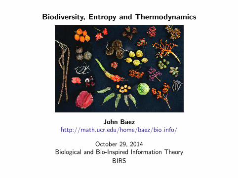
Biodiversity, Entropy and Thermodynamics

John Baezhttp://math.ucr.edu/home/baez/bio info/

October 29, 2014Biological and Bio-Inspired Information Theory

BIRS

Please apply here to attend the workshop I’m running with JohnHarte and Marc Harper:

I Information and Entropy in Biological Systems,National Institute for Mathematical and Biological Synthesis,Knoxville, Tennesee,Wednesday-Friday, 8-10 April 2015.

http://www.nimbios.org/workshops/WS entropy

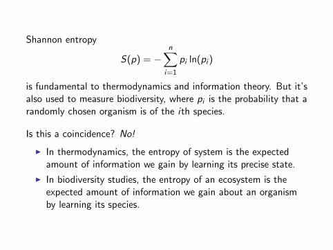
Shannon entropy

S(p) = −n∑

i=1

pi ln(pi )

is fundamental to thermodynamics and information theory. But it’salso used to measure biodiversity, where pi is the probability that arandomly chosen organism is of the ith species.

Is this a coincidence? No!

I In thermodynamics, the entropy of system is the expectedamount of information we gain by learning its precise state.

I In biodiversity studies, the entropy of an ecosystem is theexpected amount of information we gain about an organismby learning its species.

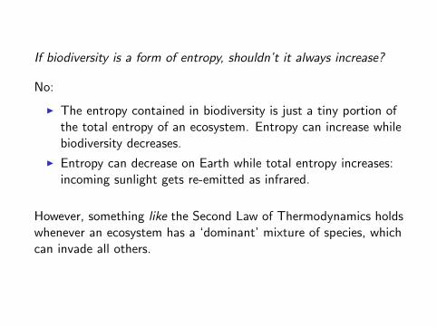
If biodiversity is a form of entropy, shouldn’t it always increase?

No:

I The entropy contained in biodiversity is just a tiny portion ofthe total entropy of an ecosystem. Entropy can increase whilebiodiversity decreases.

I Entropy can decrease on Earth while total entropy increases:incoming sunlight gets re-emitted as infrared.

However, something like the Second Law of Thermodynamics holdswhenever an ecosystem has a ‘dominant’ mixture of species, whichcan invade all others.

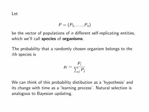
Let

P = (P1, . . . ,Pn)

be the vector of populations of n different self-replicating entities,which we’ll call species of organisms.

The probability that a randomly chosen organism belongs to theith species is

pi =Pi∑j Pj

We can think of this probability distibution as a ‘hypothesis’ andits change with time as a ‘learning process’. Natural selection isanalogous to Bayesian updating.

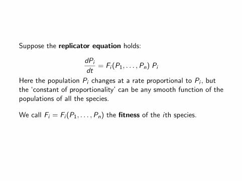
Suppose the replicator equation holds:

dPi

dt= Fi (P1, . . . ,Pn) Pi

Here the population Pi changes at a rate proportional to Pi , butthe ‘constant of proportionality’ can be any smooth function of thepopulations of all the species.

We call Fi = Fi (P1, . . . ,Pn) the fitness of the ith species.

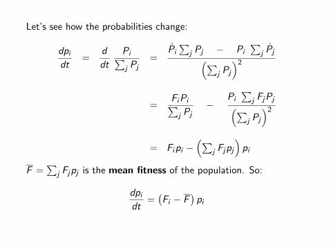
Let’s see how the probabilities change:

dpidt

=d

dt

Pi∑j Pj

=Pi∑

j Pj − Pi∑

j Pj(∑j Pj

)2=

FiPi∑j Pj

−Pi∑

j FjPj(∑j Pj

)2= Fipi −

(∑j Fjpj

)pi

F =∑

j Fjpj is the mean fitness of the population. So:

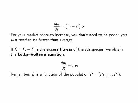
dpidt

=(Fi − F

)pi

dpidt

=(Fi − F

)pi

For your market share to increase, you don’t need to be good: youjust need to be better than average.

If fi = Fi − F is the excess fitness of the ith species, we obtainthe Lotka–Volterra equation:

dpidt

= fipi

Remember, fi is a function of the population P = (P1, . . . ,Pn).

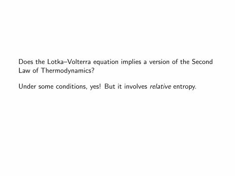
Does the Lotka–Volterra equation implies a version of the SecondLaw of Thermodynamics?

Under some conditions, yes! But it involves relative entropy.

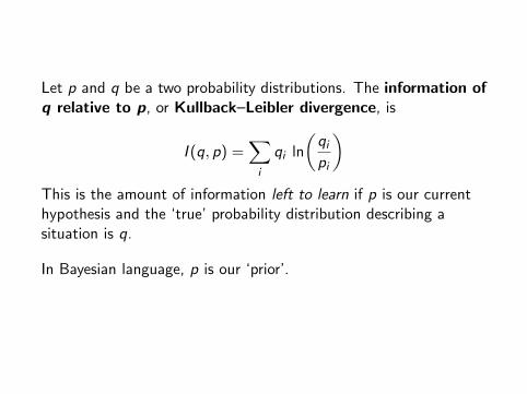
Let p and q be a two probability distributions. The information ofq relative to p, or Kullback–Leibler divergence, is

I (q, p) =∑i

qi ln

(qipi

)This is the amount of information left to learn if p is our currenthypothesis and the ‘true’ probability distribution describing asituation is q.

In Bayesian language, p is our ‘prior’.

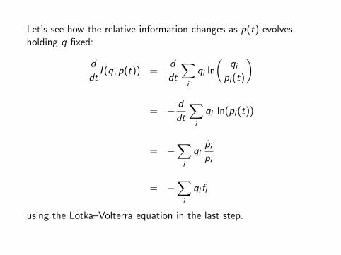
Let’s see how the relative information changes as p(t) evolves,holding q fixed:

d

dtI (q, p(t)) =

d

dt

∑i

qi ln

(qi

pi (t)

)

= − d

dt

∑i

qi ln(pi (t))

= −∑i

qipipi

= −∑i

qi fi

using the Lotka–Volterra equation in the last step.

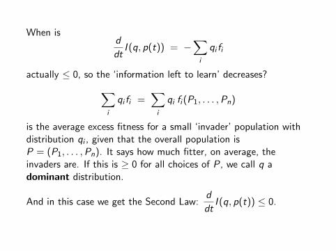
When isd

dtI (q, p(t)) = −

∑i

qi fi

actually ≤ 0, so the ‘information left to learn’ decreases?∑i

qi fi =∑i

qi fi (P1, . . . ,Pn)

is the average excess fitness for a small ‘invader’ population withdistribution qi , given that the overall population isP = (P1, . . . ,Pn). It says how much fitter, on average, theinvaders are. If this is ≥ 0 for all choices of P, we call q adominant distribution.

And in this case we get the Second Law:d

dtI (q, p(t)) ≤ 0.

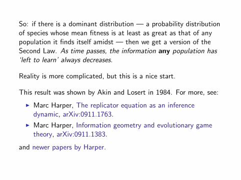
So: if there is a dominant distribution — a probability distributionof species whose mean fitness is at least as great as that of anypopulation it finds itself amidst — then we get a version of theSecond Law. As time passes, the information any population has‘left to learn’ always decreases.

Reality is more complicated, but this is a nice start.

This result was shown by Akin and Losert in 1984. For more, see:

I Marc Harper, The replicator equation as an inferencedynamic, arXiv:0911.1763.

I Marc Harper, Information geometry and evolutionary gametheory, arXiv:0911.1383.

and newer papers by Harper.