Biodiversity Inventory of Natural LandsA How-To Manual for Foresters

and Biologists

NatureServe techNical report ▪ July 2009

A product of the Forest and Biodiversity Conservation Alliance, sponsored by Office Depot

NatureServe1101 Wilson Boulevard, 15th FloorArlington, Virginia 22209703-908-1800www.natureserve.org

NatureServe is a non-profit organization dedicated to providing the scientific basis for effective conservation action.

Citation: Cutko, A. 2009. Biodiversity Inventory of Natural Lands: A How-To Manual for Foresters and Biologists. Arlington, Virginia: NatureServe.

Cover photo courtesy of Virginia Natural Heritage Program.

© NatureServe 2009

Printed on FSC-certified paper.

Office Depot provided funding for this report as part of its five-year, $2.2 million sponsorship of the Forest & Biodiversity Conservation Alliance, a collaboration among NatureServe, Conservation International and The Nature Conservancy that aims to develop the information, standards, and tools needed to advance forest and biodiversity conservation policies within the paper products supply chain. For more information, please visit www.officedepot.com/environment.

Biodiversity Inventory of Natural Lands

A How-To Manual for Foresters and Biologists

Andy CutkoCommunity Ecologist

Maine Natural Areas Program 207-287-8042

Andrew.Cutko@maine.gov(formerly: Forest Program

Officer, NatureServe)

July 2009

Funding for this project was provided by Office Depot, Inc., which is committed to promoting and advancing responsible forest management and the conservation of

forests and the biodiversity they contain.Technical review was provided by Pat Comer and Larry Master of NatureServe, Chris

Ludwig of the Virginia Division of Natural Heritage, Martina Hines of the Kentucky Natural Heritage Program, and Al Schotz of the Alabama Natural Heritage Program. Gary Beauvais and Doug Keinath of the Wyoming Natural Diversity Database provided background materials on predictive distribution modeling techniques. Rob Riordan and Marta VanderStarre of NatureServe edited, designed and produced the report.

A number of biologists and other staff from member programs of the NatureServe network provided overall guidance to this project and assistance in documenting inven-tory techniques and planning considerations. I thank the following:

Del Meidinger and Karen Yearsley, British Columbia Conservation Date Centre Bill McAvoy and Christopher Heckscher, Delaware Natural Heritage Program Kris Johnson, Natural Heritage New MexicoMark Hall, NatureServeEric Peterson Nevada Natural Heritage ProgramTim Howard, New York Natural Heritage ProgramKristen Sinclair, North Carolina Natural Heritage Program Karen Patterson, Virginia Division of Natural HeritageElizabeth Byers, West Virginia Natural Heritage Program

Special thanks to Steve Rust of the Idaho Conservation Data Center for his overall contributions to this report.

Acknowledgments

Executive Summary 1

Introduction 2

Biodiversity and Natural Heritage Inventories 2

Objectives and Organization of this Manual 3

What to Look For: Identifying and Prioritizing Target Species and Communities

5

Elements of Biodiversity 5

Conservation Status of Elements 5

Taxonomic Standards for Species 8

Classification of Natural Communities and Ecological Systems 9

Information Sources to Guide Inventory 10

Methods and Tools to Guide Inventory 14

The Coarse-filter/Fine-filter Approach to Inventory 14

Conventional Landscape Analysis Methods 14

Predictive Distribution Modeling 17

Expert Opinion Maps 17

Inventory Planning Considerations 19

Inventory and Sampling Techniques 23

Species Inventories 23

Natural Community and Vegetation Surveys 25

Collaboration with Natural Heritage Programs, Data Collection, and Reporting 27

Literature Cited 29

Glossary 31

Contents

Terms appearing in bold in the text are defined in the Glossary.

Appendices are provided in a separate document.

A current directory of U.S. natural heritage programs and Canadian conservation data centres is available on the NatureServe website at www.natureserve.org/ visitLocal/index.jsp.

Biodiversity Inventory Manual 1

Executive

Summary

With literally thousands of rare plants, animals and ecological community types to consider, the task of designing an effective biodiversity survey can be daunting. The NatureServe network maintains information on nearly

65,000 species and 6,000 ecological community types, and this information stockpile is continually expanding. However, to date there has been little consistent or uniform guidance regarding the specific tools and techniques for conducting biodiversity inven-tories. Fortunately, recent developments in remote sensing and geographic information systems (GIS) have greatly enhanced methods to screen and inventory large landscapes for biodiversity features.

This manual is intended as a practical, hands-on guide to biodiversity inventory. It provides an overview of the data sources, analytical tools and methods, and field techniques involved in surveying lands for rare species and ecological communities of concern.

Office Depot, the principal funder of this publication, is dedicated to conserving for-est biodiversity and supporting sustainable forestry efforts. To achieve this aim, Office Depot relies on sustainable forest certification standards, such as the Sustainable Forest-ry Initiative and the Forest Stewardship Council. These standards require consideration of biodiversity features such as rare species and ecological communities. As a result, this manual was inspired by an interest in forested habitats and their conservation. Nonethe-less, many of the methods and information sources described here are relevant for other landscape types as well.

Many data sources used to guide biodiversity inventory are now publicly available. These include GIS data on both biotic and abiotic landscape features (e.g., digital eleva-tion models, soils, hydrology, wetlands), land use/land cover (e.g., regional GAP cover-ages), and remote imagery (aerial photos and satellite imagery at a variety of scales). In addition, many private companies and land management agencies have their own finer-scaled natural resource data, such as forest stand and harvest maps, that significantly bolster the ability to screen areas for biodiversity inventory.

Tools for site screening range from conventional methods such as analysis of aerial photos and consulting expert opinion to innovative and evolving GIS-based techniques such as predictive distribution modeling. Although the latter techniques increasingly rely on computer algorithms to predict the locations of rare features, it is critical that they are implemented by personnel knowledgeable about the plants, animals, ecological communities and landscapes of interest.

The NatureServe network has developed a variety of field sampling techniques, plot designs, data recording protocols, and field forms that have proven successful for bio-diversity inventories. Many of these protocols are introduced here, but readers are en-couraged to consult with NatureServe member programs (i.e., U.S. natural heritage programs and Canadian conservation data centres) regarding details on techniques for specific taxa or landscape types.

Because of their local expertise, personnel of NatureServe member programs are ide-ally suited to conduct or provide guidance on biodiversity inventories at the local level. Similarly, as recipients and managers of biodiversity data, member programs are well positioned to provide the proper conservation context to the data, such as information on rarity, conservation, and management of rare species and ecological communities.

Advances in GIS capabilities, coupled with increasing availability of digital data, are rapidly improving and changing the way biodiversity inventories are conducted. Conse-quently, this manual should be considered a living document; NatureServe will update relevant inventory methods and associated links as they become available.

2 NatureServe

Introduction

Biodiversity and Natural Heritage Inventories

Commonly defined as “life in all its forms,” biodiversity represents the variety of genes, species, and ecosystems present on earth, as well as the natural pro-cesses that sustain them. This is a weighty concept to comprehend, let alone

inventory and document. At one end of the spectrum, biodiversity inventories include exhaustive “all-taxa” surveys that seek to identify the full complement of living organ-isms within an area of interest (also known as the “bio-blitz” approach). In Great Smoky Mountains National Park, for example, researchers are seeking to document the esti-mated 100,000 species known to exist within the park.

A more typical and pragmatic approach to biodiversity inventory is to target a par-ticular species, ecological community, or taxonomic group, such as all rare fish species in a particular river stretch. For decades groups such as The Nature Conservancy, Con-servation International, and the World Wildlife Fund have focused conservation efforts on rare species and habitat types, more recently expanding that focus to include intact, representative ecological communities and ecological systems. In support of these and similar efforts, NatureServe and its member programs, which collectively comprise the NatureServe network (see box, page 3), have developed systematic natural heritage in-ventory methods to document rare species and ecological communities in the Western Hemisphere. These targeted inventory methods, rather than the all-taxa surveys noted above, are the subject of this manual.

The Value of Biodiversity Inventories In light of the thousands of species and natural community types that the NatureServe network lists as of conservation concern, there are virtually no places where on-the-ground inventories of biodiversity are considered complete. This is particularly true in remote or inaccessible areas, such as large parts of Latin America and Canada. Even in reasonably well-studied places that have over a century of recorded natural history data, information on lesser-known taxa is often scarce. (The variation in inventory data is rep-resented by the appropriately named “university hot spot” phenomenon, whereby high concentrations of rare species are often found within a short drive of universities with botany or zoology departments).

Increasingly, land managers are becoming proactive about biodiversity inventories, recognizing that it is cost-effective to document hot spots in advance and incorporate them appropriately into planning, rather than wait until a conflict arises. In this regard, sound biodiversity information is critical to minimizing financial exposure caused by risks and uncertainty.

An often overlooked benefit of biodiversity inventories is that for lesser-known spe-cies, increased inventories may actually result in the downlisting of species previously thought to be rare. In Maine, for example, inventory on forest industry lands in remote parts of the state resulted in more than a dozen species, including some global rarities, being removed from the state rare-plant list. Of course, for such a downlisting to occur, it is crucial that inventory data are shared with the local natural heritage program or conservation data centre.

Biodiversity, Sustainable Forest Management and Forest CertificationConservation and management of biodiversity in forested landscapes is greatly facilitated by access to reliable information about the condition and location of at-risk species and ecological communities. As forest certification standards have evolved, biodiversity con-

Biodiversity Inventory of Natural Lands 3

cepts and criteria have increasingly been incorporated. To varying degrees the major cer-tification systems in place for North America—the Sustainable Forestry Initiative (SFI), Forest Stewardship Council (FSC), and Canadian Standards Association (CSA)—now either reference NatureServe data directly or refer more broadly to rare and endangered species and ecosystems (see box, page 4).

In forested landscapes, the identification and management of at-risk species, eco-logical communities and other ecological values are increasingly undertaken outside the scope of forest certification programs, as part of landowners’ efforts to meet the expecta-tions for long-term forest stewardship, or to meet criteria established under “working forest” conservation easements. In some states, biodiversity data are now a requirement of federally or state-funded stewardship cost-share plans.

Objectives and Organization of this Manual

This manual provides an overview of the methods and tools involved in conducting biodiversity inventories on forested landscapes. In a sense, it is an introduction to

best management practices for surveying species and ecological communities of con-cern. The methods and tools described here, which draw on the collective expertise of the hundreds of staff of the NatureServe network, have evolved during three decades of experience with biodiversity inventory. This compilation of inventory approaches is in-tended to improve the consistency and quality of inventories, reduce costs to landown-ers, improve the quality of NatureServe data, and provide new opportunities to protect occurrences of at-risk species and ecological communities.

The key components of this manual are determining what to look for, identifying the information sources to guide inventory, evaluating specific inventory methods, and documenting and reporting data. Some of these concepts were initially described by The Nature Conservancy and NatureServe in Stein and Davis (2000). This manual picks up where that document left off by providing more detailed guidance on the hands-on, practical steps involved in biodiversity inventory. This manual does not address issues of managing biodiversity data; readers should consult NatureServe for details on Biotics, our biodiversity data management system, and other data management issues (see www.natureserve.org/prodServices/biotics.jsp).

This manual was developed with multiple audiences in mind. First, recognizing Office Depot’s interest in sustainable forest management, the manual was developed for biologists and land managers working in the forest sector. As a result, it has a focus on identifying species and habitats of concern in forest landscapes, using data relevant to forestlands. However, this manual is sufficiently broad to be useful to other land man-agers and decision makers in the transportation, energy and public land management sectors. NatureServe expects its data and services to be valuable to a wide range of land-owners and managers who are responsible for maintaining at-risk species, populations and community elements of biodiversity.

Second, this manual is intended to serve as a reference for natural heritage programs. While there is considerable consistency among programs in inventory methods, the network has lacked documentation of these methods in a centralized source.

To meet the different needs of multiple audiences, the body of the text provides a high-level overview of the issues, data sources and methods involved in inventory, and a series of appendices provides additional guidance. Where additional details are merited, two types of links are provided:

The NatureServe NetworkNatureServe is a non-profit conservation organization whose mission is to provide the scientific basis for effective conservation action. NatureServe represents an international network of biologi-cal inventories—known as natural heritage programs or conserva-tion data centers—operating in all 50 U.S. states, Canada, Latin America and the Caribbean. The NatureServe network is the lead-ing source for information about rare and endangered species and threatened ecosystems. Together with these network member programs, we not only collect and manage detailed local information on plants, animals and ecosys-tems, but also develop information products, data management tools and conservation services to help meet local, national and global conservation needs.

The NatureServe Forest Program works with forest certification systems, forest industry, paper suppliers, and conservation groups to optimize the quality, accessibil-ity and value of NatureServe data and services. The Forest Program also supports the on-the-ground conservation activities of network member programs. Key initia-tives and activities include data development, data dissemination, inventory services, landscape analysis, predictive distribution modeling, use of decision-support tools in conservation planning, and forester training.

4 NatureServe

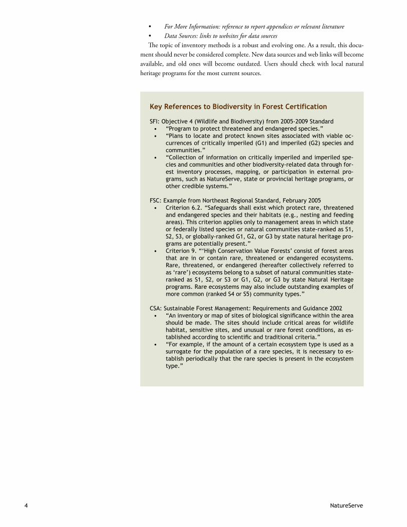
• ForMoreInformation:referencetoreportappendicesorrelevantliterature• DataSources:linkstowebsitesfordatasourcesThe topic of inventory methods is a robust and evolving one. As a result, this docu-

ment should never be considered complete. New data sources and web links will become available, and old ones will become outdated. Users should check with local natural heritage programs for the most current sources.

Key References to Biodiversity in Forest Certification

SFI: Objective 4 (Wildlife and Biodiversity) from 2005-2009 Standard“Program to protect threatened and endangered species.”•“Plans to locate and protect known sites associated with viable oc-•currences of critically imperiled (G1) and imperiled (G2) species and communities.”“Collection of information on critically imperiled and imperiled spe-•cies and communities and other biodiversity-related data through for-est inventory processes, mapping, or participation in external pro-grams, such as NatureServe, state or provincial heritage programs, or other credible systems.”

FSC: Example from Northeast Regional Standard, February 2005Criterion 6.2. “Safeguards shall exist which protect rare, threatened •and endangered species and their habitats (e.g., nesting and feeding areas). This criterion applies only to management areas in which state or federally listed species or natural communities state-ranked as S1, S2, S3, or globally-ranked G1, G2, or G3 by state natural heritage pro-grams are potentially present.” Criterion 9. “‘High Conservation Value Forests’ consist of forest areas •that are in or contain rare, threatened or endangered ecosystems. Rare, threatened, or endangered (hereafter collectively referred to as ‘rare’) ecosystems belong to a subset of natural communities state-ranked as S1, S2, or S3 or G1, G2, or G3 by state Natural Heritage programs. Rare ecosystems may also include outstanding examples of more common (ranked S4 or S5) community types.”

CSA: Sustainable Forest Management: Requirements and Guidance 2002“Aninventoryormapofsitesofbiologicalsignificancewithinthearea•should be made. The sites should include critical areas for wildlife habitat, sensitive sites, and unusual or rare forest conditions, as es-tablishedaccordingtoscientificandtraditionalcriteria.”“For example, if the amount of a certain ecosystem type is used as a •surrogate for the population of a rare species, it is necessary to es-tablish periodically that the rare species is present in the ecosystem type.”

Biodiversity Inventory Manual 5

What to Look For:

Identifying and

Prioritizing Target

Species and

Communities

Prior to initiating an inventory of a particular region, it is useful to develop or acquire a list of the species, ecological communities and ecological systems that might occur in that region. Collectively, these targets are known as elements of

biodiversity. Local natural heritage programs maintain lists of tracked elements (i.e., those elements which are documented and mapped by the programs) and should serve as the chief information source on what to look for during inventory work. The follow-ing discussion describes the methods and logic used by natural heritage programs to determine which elements are tracked.

Elements of Biodiversity

NatureServe recognizes a broad suite of biodiversity elements for potential conser-vation attention, including plant and animal species and ecological communities

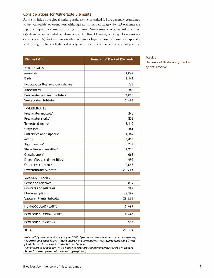
and systems. Currently NatureServe maintains information on more than 62,000 spe-cies, 7,400 ecological community types, and 680 types of ecological systems (see Table 2). These elements include virtually all vascular plants and vertebrate animal species native to the continental United States, Hawaii and Canada, major invertebrate groups, and a large proportion of non-vascular plants, as well as sizable numbers of exotic spe-cies. For a list of species and community types tracked in your state or region, contact the appropriate natural heritage program or conservation data center (CDC), listed at www.natureserve.org/visitLocal/index.jsp.

In addition to tracking animal species, subspecies and varieties, NatureServe also maintains information on transient but recurring animal assemblages, particularly for migratory species. Some migratory species occur in large multiple-species aggregations at particular places during periods in their life cycle or during their annual migrations. Examples of mixed-species animal assemblages include shorebird migratory concentra-tion areas, marine fisheries concentration areas, and bat hibernacula, all of which deserve special conservation attention.

Significant components of biodiversity remain undocumented. For example, the more than 26,000 animal species tracked in the United States are less than 15% of the number of described animal species in the country. Two-thirds of animal species are insects (approximately 100,000 species described in the U.S.), and the status and distribution of most of these are too poorly known to meaningfully assess. Other poorly described animal groups include most crustaceans, arachnids, flatworms, annelids and nematodes, although there are exceptions within some of these groups (e.g., crayfishes and cave-obligate species).

Likewise, less charismatic groups such as microbes or non-lichenized fungi have not yet been comprehensively assessed. Thus, the conservation of rare species in these groups depends upon the conservation of associated “coarse-filter” elements and co-occurring rare species in better-known groups.

For More Information:• ForadetailedassessmentofthedatatrackedbyNatureServe,seeBrownetal.(2004),availableatwww.natureserve.org/library/ncasi_report.pdf.

Conservation Status of Elements

Conservation status ranks, which reflect the rarity of elements at the global, na-tional or state/provincial level, are one of the principal factors for determining

which elements should be targeted for surveys. NatureServe has developed a consistent method for assessing the conservation status of species, ecological communities and ecological systems. This methodology leads to the designation of a conservation status

6 NatureServe

TABLE 1NatureServe Global Conservation Status Ranks

rank, which for species provides an initial estimate of the risk of extinction or extirpa-tion (Master et al. 2003). (NatureServe is currently assessing the similarities between its global ranking conventions and those used by the IUCN-World Conservation Union’s Red List Programme, with some consideration directed toward adoption of the IUCN system by NatureServe.)

Conservation status ranks are based on a scale of one to five, ranging from criti-cally imperiled range-wide (G1) to demonstrably secure (G5) (see Table 1). Species presumed to be extinct are ranked GX, while those considered missing and possibly ex-tinct are ranked GH. NatureServe global or range-wide conservation status assessments (designated “G” for global) are augmented by national (“N”) and state/provincial/ter-ritorial (“S” for subnational) conservation status assessments. National ranks are more commonly used in Latin America due to the presence of country-wide CDCs and the lack of sub-national status assessments..

For ecological communities, conservation status ranks provide an initial estimate of relative rarity, along with trends in the overall abundance and quality of all occurrences. While rankings are fairly complete for associations, classification of ecological systems has only recently been completed for the United States (and has not yet begun in Cana-da), so conservation status assessments for systems have not yet been developed.

In biodiversity-rich areas (e.g., places with many endemic species, such as Hawaii), inventory and documentation efforts will likely focus on only the rarest elements from a global perspective. Consequently, G1, G2 and GH elements will always be included on inventory target lists. In many parts of North America, efforts also focus on elements that are rare within a jurisdiction (e.g., S1-S3 elements) and high-quality examples of common (S4 and S5) ecological communities or systems.

Rank1 Description

GX Presumed Extinct. Not located despite intensive searches and virtually no likelihood of rediscovery.

GH Possibly Extinct. Missing; known from only historical occurrences but still some hope of rediscovery.

G1 Critically Imperiled. At very high risk of extinction due to ex-treme rarity (often 5 or fewer populations), very steep declines, or other factors.

G2 Imperiled. At high risk of extinction due to very restricted range, very few populations (often 20 or fewer), steep declines, or other factors.

G3 Vulnerable.Atmoderateriskofextinctionorofsignificantconservation concern due to a restricted range, relatively few populations (often 80 or fewer), recent and widespread declines, or other factors.

G4 Apparently Secure. Uncommon but not rare; some cause for long-term concern due to declines or other factors.

G5 Secure. Common; widespread and abundant.

1Note: “G” refers to global or range-wide conservation status for a species or ecological community. Infra-specific taxa (subspecies, varieties and populations) are given an equivalent “T” ranking. For example, the conservation status ranking for an imperiled subspecies of a globally secure species would be G5T2.

Biodiversity Inventory of Natural Lands 7

Considerations for Vulnerable ElementsAt the middle of the global ranking scale, elements ranked G3 are generally considered to be ‘vulnerable’ to extinction. Although not imperiled rangewide, G3 elements are typically important conservation targets. In most North American states and provinces, G3 elements are included on element tracking lists. However, tracking all element oc-currences (EOs) for G3 elements often requires a large amount of resources, especially in those regions having high biodiversity. In situations where it is currently not practical

Element Group Number of Tracked Elements

VERTEBRATES

Mammals 1,047

Birds 1,163

Reptiles, turtles, and crocodilians 722

Amphibians 388

Freshwaterandmarinefishes 2,096

Vertebrates Subtotal 5,416

INVERTEBRATES

Freshwater mussels* 340

Freshwater snails* 835

Terrestrial snails* 2,110

Crayfishes* 381

Butterfliesandskippers* 1,389

Moths 3,452

Tiger beetles* 272

Stonefliesandmayflies* 1,225

Grasshoppers* 669

Dragonfliesanddamselflies* 495

Other invertebrates 10,045

Invertebrates Subtotal 21,213

VASCULAR PLANTS

Ferns and relatives 839

Conifers and relatives 187

Flowering plants 28,199

Vascular Plants Subtotal 29,225

NON-VASCULAR PLANTS 6,429

ECOLOGICAL COMMUNITIES 7,420

ECOLOGICAL SYSTEMS 686

TOTAL 70,389

Note: All figures current as of August 2007. Species numbers include tracked subspecies, varieties, and populations. Totals include 244 vertebrates, 152 invertebrates and 3,948 plants known to be exotic in the U.S. or Canada. * Invertebrate groups for which native species are comprehensively covered in Nature-Serve Explorer (www.natureserve.org/explorer).

TABLE 2Elements of Biodiversity Tracked by NatureServe

8 NatureServe

to track all the occurrences of G3 elements, many programs chose to track all elements with “A” or “B” occurrence ranks, particularly for ecological communities.

Considerations for Common ElementsAt the other end of the rarity spectrum, elements ranked G4 and G5 are generally considered to be widespread, abundant and at least apparently secure. They are rarely subjected to serious threats throughout their range. However, many G4 and G5 ele-ments, such as an oak-hickory forest in Nova Scotia or a northern hardwood forest in Virginia, are rare or vulnerable at the edges of their range. Decisions on tracking occurrences of G4 and G5 species are based on biogeographic context as well as local considerations. In contrast, outstanding examples of G4 and G5 natural communities or ecological systems should always be included on a target list. In places where they are most widespread or abundant, emphasis should be placed on tracking the highest-qual-ity examples (i.e., those with occurrence ranks of A or B).

Biogeographic Considerations To generate a list of species or natural communities that may occur in a study area, it is often useful to first overlay species or community range maps with study area boundar-ies. Surveyors should also consider species or communities that may occur in a study area but are currently not known from it; these might include species ranked “SH” (historic), “SR” (reported), or others known from adjacent jurisdictions. In addition, it is useful to consider the broad habitat types present in the region and the species or natural communities that those habitat types may support. Staff knowledge within natural heritage programs and CDCs is invaluable in this regard.

IrreplaceabilityTo maximize the conservation effectiveness of inventories, it is often desirable to priori-tize species and communities according to their “irreplaceability.” In addition to con-servation status, irreplaceability involves considerations of taxonomic uniqueness, geo-graphic isolation and representation, and endemism. The Alliance for Zero Exinction, for example, focuses on sites that are truly irreplaceable because their loss will result in the extinction of a species. Irreplaceability may also require explicit consideration of seasonal differences for migratory taxa. Some shorebirds, waterfowl and cranes may be widespread and abundant on breeding and wintering grounds but are constrained to only a few stopover sites (e.g., concentration areas or “bottlenecks”) during migration. These stopover sites are then “irreplaceable” for the viability of these species.

Taxonomic Standards for Species

In an effort to simplify the complexities of the natural world, scientists impose struc-ture or organization on dynamic living systems by classifying them into like groups.

Multiple levels of living systems have been classified, ranging from cells to species, natu-ral communities, landscapes, and biomes. In any classification system, it is necessary to portray shades of gray as black and white in order to find order in nature’s complexity.

The species concepts and names recognized by NatureServe are primarily obtained from standardized lists widely accepted among researchers with expertise in given groups (e.g., the American Ornithologists’ Union Check-List of North American Birds and Kartesz’s list of North American vascular plants). NatureServe currently maintains species data for all North American vertebrate animals as well as all species in the fol-lowing invertebrate groups: freshwater and terrestrial mollusks, butterflies and skippers,

Biodiversity Inventory of Natural Lands 9

crayfishes, tiger beetles, dragonflies and damselflies, grasshoppers, stoneflies, and may-flies. Records are also maintained for approximately 10,000 invertebrates in other mis-cellaneous groups and all mammals, birds and amphibians in the Western Hemisphere.

Classification of Natural Communities and Ecological Systems

Numerous natural community and ecosystem classifications exist at international, national, state and local scales (Grossman et al. 1998). Such classifications serve

multiple purposes in conservation planning and help to ensure that the full range of global and regional habitats is conserved. From a research perspective, by describing, classifying, mapping and managing ecological communities, researchers and managers are able to track and monitor a complex suite of interactions that are not recognizable through other means (Whittaker 1962; Cowardin et al. 1979; Eyre 1980; Brown 1982; Reshske 1990; McPeek and Miller 1996; Kimmins 1997).

Over the past two decades, scientists from a variety of agencies, organizations and institutions have helped to establish an ecological community classification based on vegetation, known as the International Vegetation Classification (IVC). The ecologi-cal association, which ranges in scale from less than an acre (for “small patch” types) to thousands of acres (for “matrix” types), is the fundamental inventory and planning unit of the IVC. Efforts are underway in Canada to develop vegetation types using the IVC framework (Ponomarenko and Alvo 2000; Alvo and Ponomarenko 2003).

In the U.S. and Latin America, the mid-fine-scaled ecological systems classification is a relatively new approach to describe landscapes that integrates vegetation composition and structure with characteristic environmental setting and disturbance dynamics. In the United States, these units are also used to consistently map U.S. National Vegetation Classification (NVC) alliances and associations, which are part of the federal vegeta-tion classification standard. For landscape planning at large scales, such as on national forests or private lands greater than 5,000 ha, the ecological systems scale may be most appropriate for inventory. Field inventories may be directed at identifying both the as-sociation and system levels, while remote inventories will be most effective for ecological systems.

In addition to these national and international classification efforts, many states in the eastern and midwestern U.S. have developed their own classifications for describing and tracking ecological communities. In some cases these state classifications are finer in scale than NVC associations (i.e., one NVC type = multiple state types), and in other cases the state classifications are broader (one state type = multiple NVC types). How-ever, in almost all cases the state classifications have been linked or “cross-walked” to NVC types, enabling some types of analyses at broader ecoregional or national scales.

For ecological communities, the SFI Standard for G1 and G2 elements relies on the association units of the IVC. More than 1,600 associations in the U.S. and 100 associa-tions in Canada meet the criteria for G1 or G2 elements. The relatively low number of G1 and G2 associations listed for Canada primarily reflects the incompleteness of the Canadian classification. Many more units are yet to be fully described and standard-ized. In addition to the SFI Standard, several regional standards of the Forest Certifica-tion Council reference protection of natural communities, including S1-S3 types, under Principles 6 and 9.

For More Information: • SeeAppendixBfordetailsonecologicalclassification.FormoreinformationonstateclassificationsandlinkagestotheNVC,contactyourlocalnaturalheritageprogram.

10 NatureServe

Information

Sources to

Guide Inventory

In the last decade, many data sources required for biodiversity inventory, and in some cases the processes and tools employed to analyze them, have become automated through Geographic Information Systems (GIS) and are available through various

public web portals. The recently developed Conservation Geoportal (www.conserva-tionmaps.org), for example, is a collaborative effort by the conservation community to facilitate the use of spatial data layers to support conservation decisions. It is primarily a data catalog intended to provide a listing of spatial data sets and map services relevant to biodiversity conservation.

As the availability of GIS data continues to expand, the information sources and websites listed below should be considered an illustrative, but by no means comprehen-sive, list of the types of data currently available.

Natural Heritage Program/CDC Data. Element Occurrence Records (EORs) are docu-mented records that may result from biological surveys by natural heritage programs or contractors, museum specimens, or credible reports from other biologists. The amount and coverage of this information varies widely throughout North America, reflecting the extent of past surveys. While natural heritage data is generally the most comprehensive available, the quality of this information (date last observed, mapping precision, popula-tion status, viability rank) can vary substantially across the network.

EOR data can be useful in multiple ways. First, it is a good starting point (together with range maps) to determine what elements are likely to occur in a given geographic area. Second, inspection of EORs may inform a type of search image or deductive model that predicts what landscape features are associated with the element. Third, certain descriptive fields within the EOR provide information on the associated species and natural communities for the element. These associated species and natural communities in turn improve the search image for that particular element.

Natural heritage programs also may have other ancillary information that may pro-vide useful guidance, such as observation plots and points, negative survey forms, and informal leads (known locations with insufficient data to map).

Data Source:• ContactyourlocalnaturalheritageprogramorCDCregardinguseofelementoccurrenceorothernaturalheritagedata.

Museum Collections. In many locations museum and herbaria specimens for rare species have already been incorporated into natural heritage program datasets. However, mu-seum specimens may also be useful at identifying locations of indicator species or habitat specialists that may suggest a certain habitat for rare species or natural communities. For example, if you are interested in locating the rare showy lady’s slipper (Cyprepediumreginae), and you know they are often found in the same habitats as yellow lady’s slippers (Cyprepediumpubescens), museum specimens for the latter may be instructive in finding the former.

Data Sources:• Contactyourstatenaturalheritageprogramtodetermineifmuseumspecimensforrarespecieshavebeenincorporatedintotheirdatabase.Insomestates,herbariacollectionsarealsoavailableonline.

Topography and Elevation. Historically, hard-copy maps served as a baseline for initial mapping of target areas. As GIS technology has developed, scanned USGS maps or Digital Elevation Models (DEMs) have replaced hard-copy maps. Topographic maps indicate obvious landscape features and landforms that may be correlated with certain natural community types, such as floodplain forests, cliffs, mountain summits, ravines (“cove forests”), and wetland complexes. DEM data are available for most USGS quads at a 30m resolution from USGS. Analysis of DEM data serves as an efficient and system-

Biodiversity Inventory of Natural Lands 11

atic way to identify areas with certain slope, aspect, and elevation characteristics. DEMs may also be used to model certain landform characteristics and derive general moisture flow patterns across a study area.

Data Sources: ElevationDerivativesforNationalApplication:• http://edna.usgs.govGlobal30Arc-SecondElevationDataSet:• http://eros.usgs.gov/products/eleva-tion/gtopo30.htmlNationalElevationDataset:• http://ned.usgs.gov/NedUSGSDigitalLineGraphs:• http://edc.usgs.gov/products/map/dlg.htmlUSGSDigitalRasterGraphics:• http://topomaps.usgs.gov/drg

Remote Sensing Imagery. The increased availability and reduced cost of high-quality satellite imagery have significantly enhanced the efficiency of landscape analysis. While coarse-scale imagery (e.g., 10-meter Landsat TM) may be useful for detecting unfrag-mented blocks and broad forest conditions such as recent clearcuts versus mature stands or deciduous versus coniferous stands, finer-scaled imagery (less than 5-meter, such as IKONOS) is often needed to determine habitat conditions such as forest structure.

Data Sources: AdvancedVeryHighResolutionRadiometer:• http://noaasis.noaa.gov/NOAA-SIS/ml/avhrr.htmlAirborneVisible/InfraredImagingSpectrometer:• http://aviris.jpl.nasa.gov/EarthObserving-1(EO-1,Hyperion):• http://eo1.gsfc.nasa.gov;http://eo1.gsfc.nasa.gov/new/general/firsts/hyperion.htmlLandSatOrtho-rectifiedETM+andTM:• http://edcsns17.cr.usgs.gov/nsdp/ModerateResolutionImagingSpectroradiometer:• http://modis.gsfc.nasa.gov/RADARSAT:• http://msl.jpl.nasa.gov/QuickLooks/radarsatQL.htmlSPOTImagery:• http://www.spot.com

Air photos. Depending on the scale and season of photography, air photos may be instrumental in identifying certain forest or wetland types, forest or wetland condition (i.e., forest structure, as indicated by tree crowns), harvest history, ecological commu-nity patterns, fragmentation, access, and a number of other important features. For large areas (several hundred thousand to millions of acres), for instance, National Aerial Photography Program (NAPP) color-infrared photos at a scale of 1:40,000 are available from USGS.

Data Sources: DigitalOrthophotoQuadrangles:• http://edcwww.cr.usgs.gov/products/aerial/doq.html;http://data.geocomm.com/doqqNationalAerialPhotographyProgram:• http://edc.usgs.gov/guides/napp.html

Digital Land Use/Land Cover Data. Where remote imagery has been classified to land use and land cover types, that data may be useful to identify areas that should receive more focus through analysis of finer-scaled remote imagery. Digital land use data may be available from multiple sources, including state GAP programs (USFWS), nation-wide “Medium Resolution Land Cover” (EPA), or others. When used in conjunction with other information such as elevation and soils data (where available), digital land cover data becomes a more potent tool for modeling the possible location for specific community types. Digital land use/land cover and cover type data is the primary source of ecological systems layers currently being developed by many organizations.

12 NatureServe

Data Sources: LandCoverDigitalDataDirectoryfortheUnitedStates:• http://www.epa.gov/owow/watershed/pdf/watershed_landcover.pdfNationalLand-CoverPatternData(NLCPD):• http://www.forestthreats.org/about/fhm/landscapes/nlcd-dataNationalLandCoverData(NLCD):•

http://www.epa.gov/mrlc/nlcd.htmlhttp://landcover.usgs.gov/natllandcover.phphttp://www.mrlc.gov/mrlc2k_nlcd.asp

MODISNormalizedDifferenceVegetativeIndex(NDVI):• http://modis-atmos.gsfc.nasa.gov/NDVI/index.html

Roads Data. Digital roads data may be used in conjunction with digital land cover data to identify high-quality, unfragmented or roadless areas for further analysis. Road data may also be an important source for determining future fragmentation and develop-ment threats to an area (e.g., through a build-out analysis).

Data Source: • U.S.CensusRoadData:http://www.esri.com/data/download/census2000_tigerline/index.html

National Wetlands Inventory Maps. These maps may be useful at identifying different wetland types within a larger wetland complex. Since most NWI mapping has been conducted using 1:58,000 air photos, careful review and interpretation of 1:40,000 NAPP photos may yield just as much or more information.

Data Source: • http://www.fws.gov/nwi/

Bedrock and Surficial Geologic Maps. Bedrock geology maps are particularly useful at identifying areas of uncommon parent material (e.g., calcareous or circumneutral bed-rock in parts of the northeastern U.S.). Surficial geologic maps may be used to pinpoint areas of noteworthy landforms or broad substrate types (e.g., glacial outwash plains, eskers, etc.).

Data Source:• GeneralizedGeologicMapoftheU.S.:http://pubs.usgs.gov/at-las/geologic/

Soil Surveys and Maps. The Natural Resource Conservation Service supports two publicly available digital databases: Soil Survey Geographic Database (SSURGO) and State Soil Geographic Database (STATSGO). SSURGO is the more spatially precise layer and may be preferable for use in inventories of smaller regions (e.g., a few coun-ties). STATSGO, renamed as the Digital General Soil Map of the United States, is the more generalized layer that may be preferable for use at the statewide scale or broader. STATSGO was created at a 1:250,000 scale and has a minimum mapping unit of ap-proximately 1,500 acres, with each unit containing up to 21 component soil types. A primary weakness of STATSGO is introduced in regions of more complex topography, where heterogeneous soil polygons have been combined into single units.

Data Sources: • StateandLocalSoilDatasets:http://soildatamart.nrcs.usda.gov/http://www.soils.usda.gov/survey/geography/statsgohttp://soils.usda.gov/technical/classification/scfile/index.html

Ecological Land Types. In some regions combinations of landform (slope, aspect, shape), elevation, and substrate (soils and geology) have been digitally combined to form eco-logical land types, also known as ecological land units. These units may then be cor-related with natural communities or ecological system types, using known affinities,

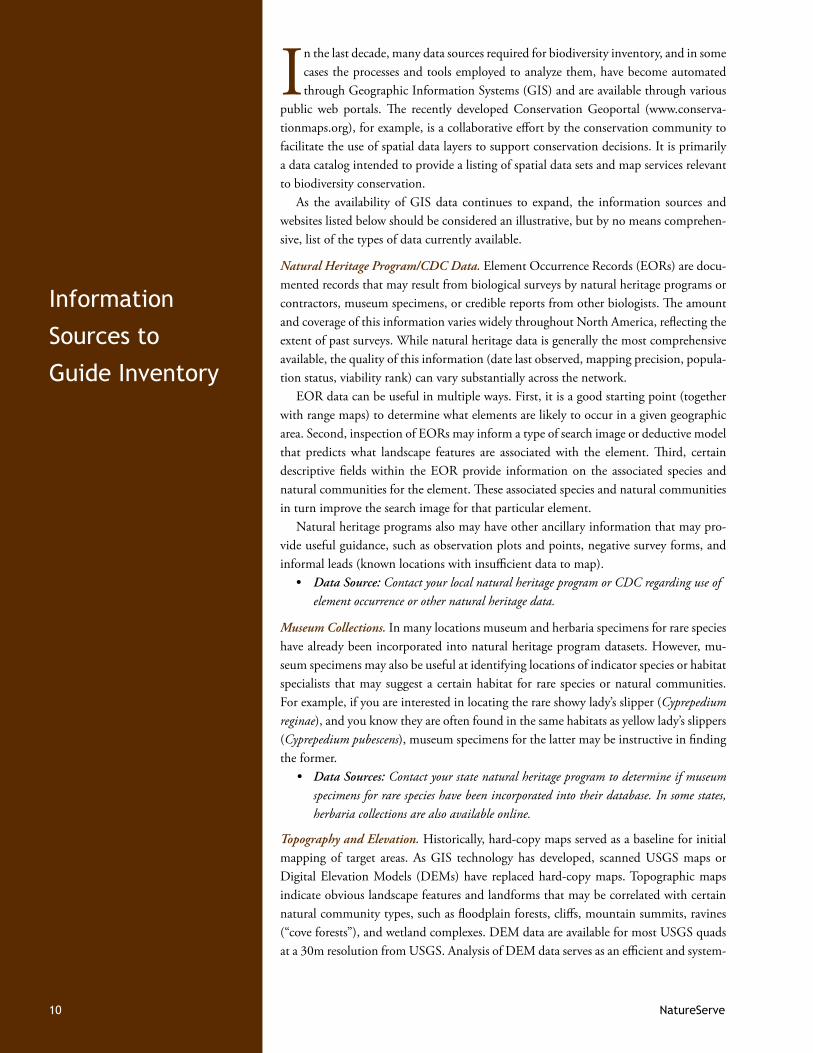
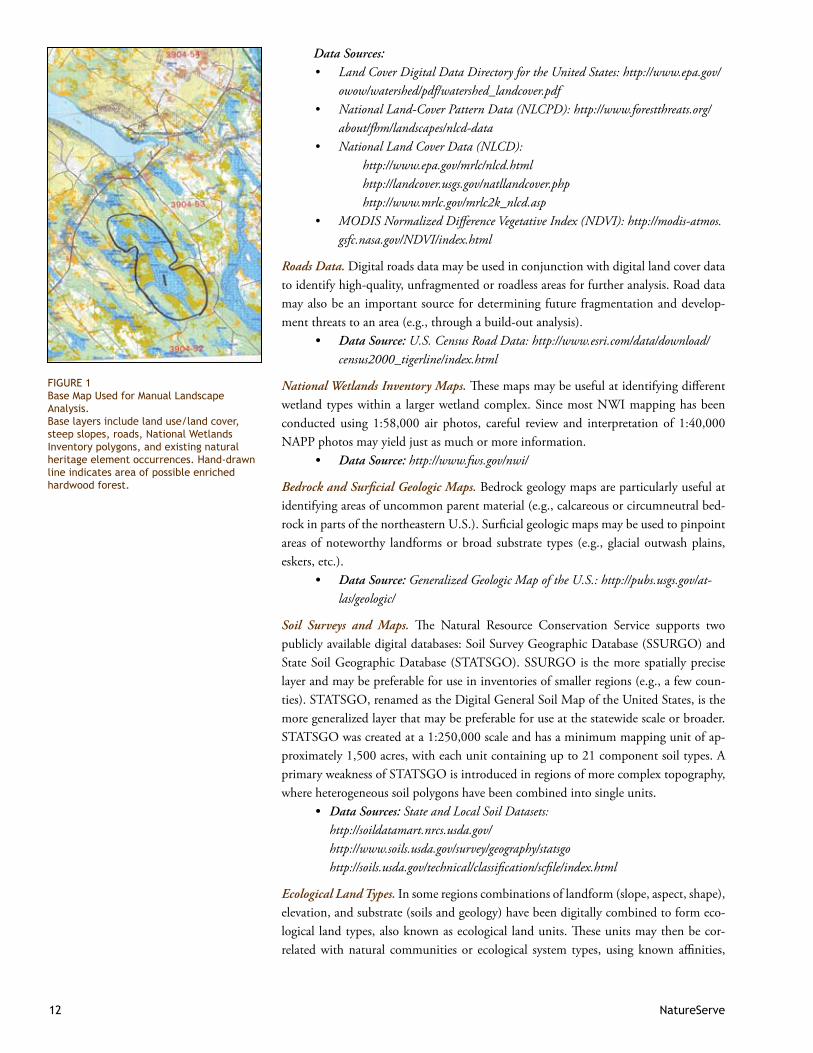
FIGURE 1Base Map Used for Manual Landscape Analysis. Base layers include land use/land cover, steep slopes, roads, National Wetlands Inventory polygons, and existing natural heritage element occurrences. Hand-drawn line indicates area of possible enriched hardwood forest.

Biodiversity Inventory of Natural Lands 13

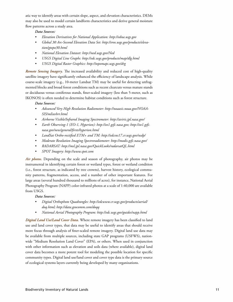
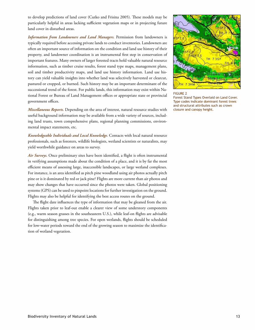
FIGURE 2Forest Stand Types Overlaid on Land Cover. Type codes indicate dominant forest trees and structural attributes such as crown closure and canopy height.

to develop predictions of land cover (Cutko and Frisina 2005). These models may be particularly helpful in areas lacking sufficient vegetation maps or in projecting future land cover in disturbed areas.

Information from Landowners and Land Managers. Permission from landowners is typically required before accessing private lands to conduct inventories. Landowners are often an important source of information on the condition and land use history of their property, and landowner coordination is an instrumental first step in conservation of important features. Many owners of larger forested tracts hold valuable natural resource information, such as timber cruise results, forest stand type maps, management plans, soil and timber productivity maps, and land use history information. Land use his-tory can yield valuable insights into whether land was selectively harvested or clearcut, pastured or cropped, or burned. Such history may be an important determinant of the successional trend of the forest. For public lands, this information may exist within Na-tional Forest or Bureau of Land Management offices or appropriate state or provincial government offices.

Miscellaneous Reports. Depending on the area of interest, natural resource studies with useful background information may be available from a wide variety of sources, includ-ing land trusts, town comprehensive plans, regional planning commissions, environ-mental impact statements, etc.

Knowledgeable Individuals and Local Knowledge. Contacts with local natural resource professionals, such as foresters, wildlife biologists, wetland scientists or naturalists, may yield worthwhile guidance on areas to survey.

Air Surveys. Once preliminary sites have been identified, a flight is often instrumental in verifying assumptions made about the condition of a place, and it is by far the most efficient means of assessing large, inaccessible landscapes, or large wetland complexes. For instance, is an area identified as pitch pine woodland using air photos actually pitch pine or is it dominated by red or jack pine? Flights are more current than air photos and may show changes that have occurred since the photos were taken. Global positioning systems (GPS) can be used to pinpoint locations for further investigation on the ground. Flights may also be helpful for identifying the best access routes on the ground.

The flight date influences the type of information that may be gleaned from the air. Flights taken prior to leaf-out enable a clearer view of some understory components (e.g., warm season grasses in the southeastern U.S.), while leaf-on flights are advisable for distinguishing among tree species. For open wetlands, flights should be scheduled for low-water periods toward the end of the growing season to maximize the identifica-tion of wetland vegetation.

14 NatureServe

Methods and

Tools to Guide

Inventory

The Coarse-filter/Fine-filter Approach to Inventory

A multi-tiered focus on ecological communities and systems (i.e., the coarse-filter elements of biodiversity) and on rare species (i.e., the fine-filter elements) forms a

coarse-filter/fine-filter approach to the identification and conservation of biological di-versity. This approach is based on the assumption that the coarse-filter approach will suc-cessfully conserve 80-95% of the biodiversity, while specific targeted actions are needed to protect the remaining species (Jenkins 1985, Maine Department of Inland Fisher-ies and Wildlife 2005). Consequently, the identification and conservation of fine- and coarse-filter elements of biodiversity across a landscape should efficiently conserve the ecological functions, processes and dynamics that support the overwhelming proportion of biodiversity in an area.

Conventional Landscape Analysis Methods

Landscape analysis is the traditional process by which biologists and ecologists iden-tify areas likely to support rare natural communities, outstanding examples of com-

mon communities, and/or habitat for rare plants. It is a common form of deductive modeling in which multiple data layers are overlaid and compared with air photos or other information to produce maps of targeted areas for field surveys. Prior to about 2000, this process was conducted manually, but in the last decade many of the manual components have been facilitated by GIS analyses, and in some cases this process has been almost entirely automated through tools such as predictive distribution modeling. In contrast to predictive approaches conducted for individual species, landscape analysis may be done collectively for a subset or for all the target elements within a study area.

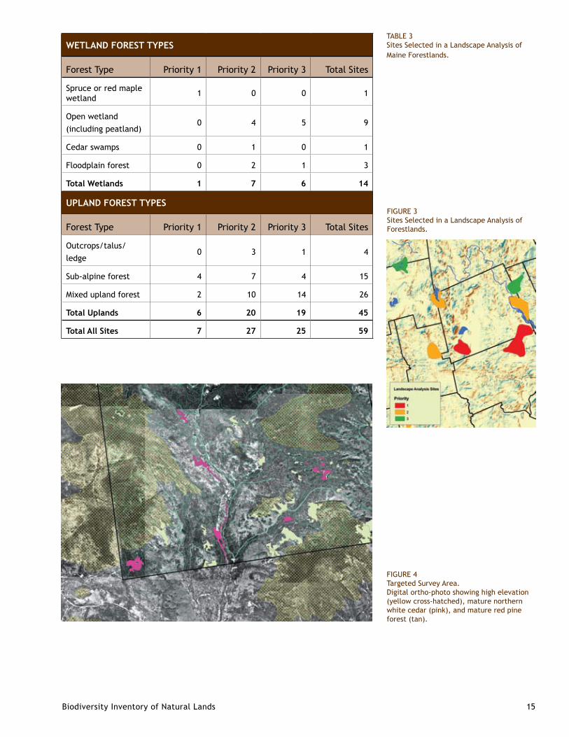
Because of the strong need for interpretation by a knowledgeable researcher, most landscape analyses are conducted using a combination of GIS-based and manual ap-proaches. Typically GIS base maps are generated and then reviewed, compared with air photos, and marked up by surveyors using local knowledge. The decision of how to interpret and weight different data layers depends on the type and scale of available data and the targeted elements. For example, high-resolution land cover or forest type data would be important for pinpointing uncommon forest communities but unnec-essary for identifying potential rivershore rare plant sites. Conversely, stream gradient and water quality might be important predictors for rare mussel species but irrelevant for rare forest types. Using some of the data layers described in the previous section of this manual, Figure 4 depicts how an ecologist might target an area to survey for intact northern white cedar or red pine natural communities.

Depending on the scale of the landscapes to be inventoried, and the species, com-munity types, or ecological systems of interest, sites targeted for field surveys may range from only a few acres to thousands of acres.

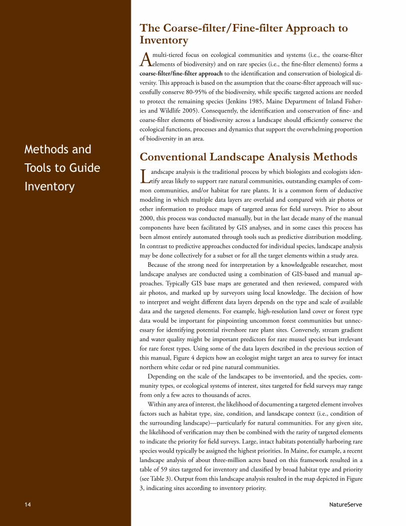
Within any area of interest, the likelihood of documenting a targeted element involves factors such as habitat type, size, condition, and lansdscape context (i.e., condition of the surrounding landscape)—particularly for natural communities. For any given site, the likelihood of verification may then be combined with the rarity of targeted elements to indicate the priority for field surveys. Large, intact habitats potentially harboring rare species would typically be assigned the highest priorities. In Maine, for example, a recent landscape analysis of about three-million acres based on this framework resulted in a table of 59 sites targeted for inventory and classified by broad habitat type and priority (see Table 3). Output from this landscape analysis resulted in the map depicted in Figure 3, indicating sites according to inventory priority.

Biodiversity Inventory of Natural Lands 15

TABLE 3 Sites Selected in a Landscape Analysis of Maine Forestlands.

FIGURE 4 Targeted Survey Area. Digital ortho-photo showing high elevation (yellow cross-hatched), mature northern white cedar (pink), and mature red pine forest (tan).

WETLAND FOREST TYPES

Forest Type Priority 1 Priority 2 Priority 3 Total Sites

Spruce or red maple wetland 1 0 0 1

Open wetland (including peatland)

0 4 5 9

Cedar swamps 0 1 0 1

Floodplain forest 0 2 1 3

Total Wetlands 1 7 6 14

UPLAND FOREST TYPES

Forest Type Priority 1 Priority 2 Priority 3 Total Sites

Outcrops/talus/ledge

0 3 1 4

Sub-alpine forest 4 7 4 15

Mixed upland forest 2 10 14 26

Total Uplands 6 20 19 45

Total All Sites 7 27 25 59

FIGURE 3 Sites Selected in a Landscape Analysis of Forestlands.

16 NatureServe

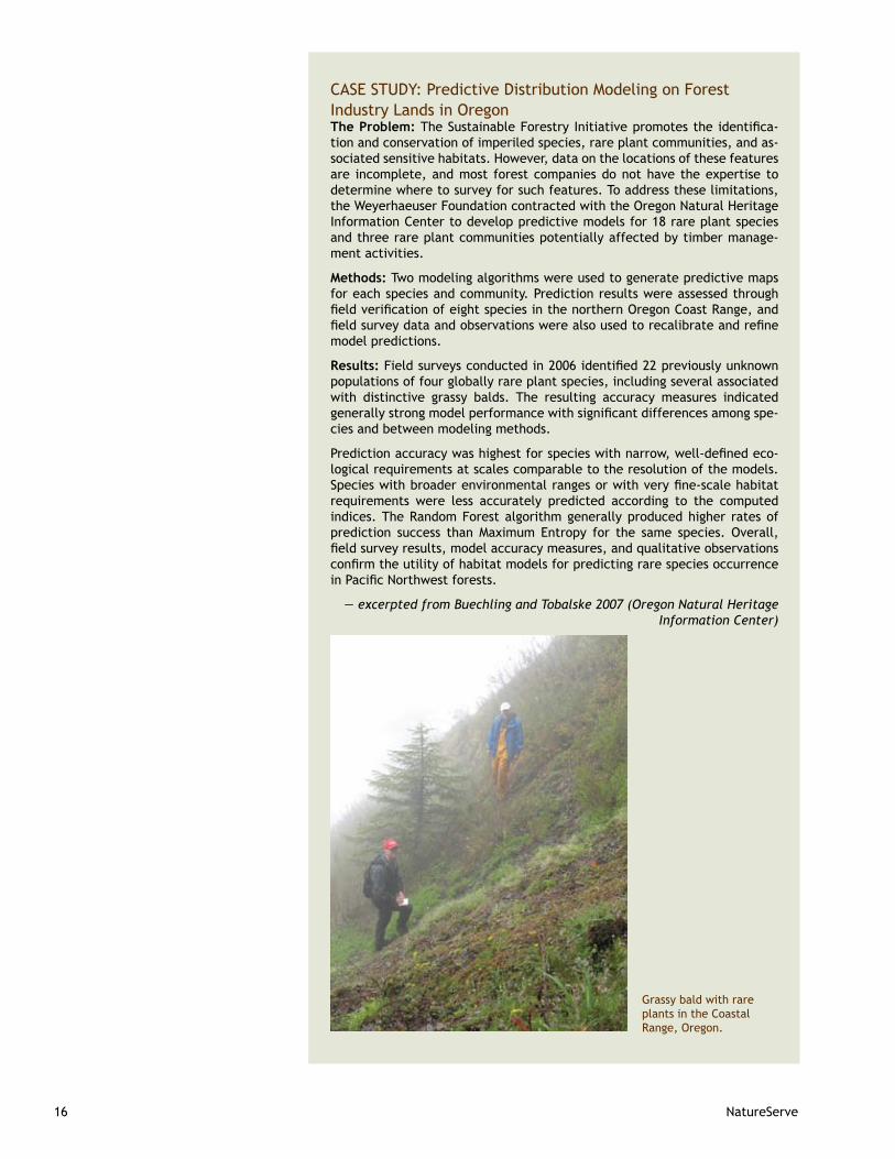
CASE STUDY: Predictive Distribution Modeling on Forest Industry Lands in Oregon The Problem: TheSustainableForestry Initiativepromotestheidentifica-tion and conservation of imperiled species, rare plant communities, and as-sociated sensitive habitats. However, data on the locations of these features are incomplete, and most forest companies do not have the expertise to determine where to survey for such features. To address these limitations, the Weyerhaeuser Foundation contracted with the Oregon Natural Heritage Information Center to develop predictive models for 18 rare plant species and three rare plant communities potentially affected by timber manage-ment activities.

Methods: Two modeling algorithms were used to generate predictive maps for each species and community. Prediction results were assessed through fieldverificationofeightspeciesinthenorthernOregonCoastRange,andfieldsurveydataandobservationswerealsousedtorecalibrateandrefinemodel predictions.

Results: Fieldsurveysconductedin2006identified22previouslyunknownpopulations of four globally rare plant species, including several associated with distinctive grassy balds. The resulting accuracy measures indicated generallystrongmodelperformancewithsignificantdifferencesamongspe-cies and between modeling methods.

Predictionaccuracywashighestforspecieswithnarrow,well-definedeco-logical requirements at scales comparable to the resolution of the models. Specieswithbroaderenvironmentalrangesorwithveryfine-scalehabitatrequirements were less accurately predicted according to the computed indices. The Random Forest algorithm generally produced higher rates of prediction success than Maximum Entropy for the same species. Overall, fieldsurveyresults,modelaccuracymeasures,andqualitativeobservationsconfirmtheutilityofhabitatmodelsforpredictingrarespeciesoccurrenceinPacificNorthwestforests.

— excerpted from Buechling and Tobalske 2007 (Oregon Natural Heritage Information Center)

Grassy bald with rare plants in the Coastal Range, Oregon.

Biodiversity Inventory of Natural Lands 17

Predictive Distribution Modeling

Predictive Distribution Modeling (PDM) is a relatively new GIS-based procedure that uses known habitat preferences of species or communities to predict addi-

tional possible occurrences. It has high potential to increase the efficiency of inventory and conservation projects in large landscapes where comprehensive, conventional field inventory efforts are not practical. PDM is based on the assumption that species and natural communities are linked to the landscape by recognizable biotic and abiotic predictors. Accordingly, PDM is a much more accurate method of estimating occur-rences than most more coarsely-scaled existing range or distribution maps developed by traditional methods. While the underlying concepts behind distribution modeling are not new, only recently have advances in GIS technology and remote-sensing enabled this technique to gain widespread application (Guisan and Zimmerman 2000, Rushton et al. 2004).

In addition to predicting element locations, PDM may also be used to suggest areas of negative occurrence (that is, maps showing where species or communities are not likely to occur). This ability to provide greater certainty about “negative” data is impor-tant for numerous forestry and development applications. In addition, PDM predic-tions do not necessarily need to be categorized as suitable or unsuitable but may depict suitability in varying degrees or gradients from “high” to “low.”

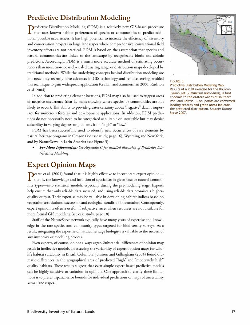
PDM has been successfully used to identify new occurrences of rare elements by natural heritage programs in Oregon (see case study, page 16), Wyoming and New York, and by NatureServe in Latin America (see Figure 5) .

For More Information:• SeeAppendixCfordetaileddiscussionofPredictiveDis-tributionModeling.

Expert Opinion Maps

Pearce et al. (2001) found that it is highly effective to incorporate expert opinion—that is, the knowledge and intuition of specialists in given taxa or natural commu-

nity types—into statistical models, especially during the pre-modeling stage. Experts help ensure that only reliable data are used, and using reliable data promises a higher-quality output. Their expertise may be valuable in developing habitat indices based on vegetation associations, succession and ecological condition information. Consequently, expert opinion is often a useful, if subjective, asset when resources are not available for more formal GIS modeling (see case study, page 18).

Staff of the NatureServe network typically have many years of expertise and knowl-edge in the rare species and community types targeted for biodiversity surveys. As a result, integrating the expertise of natural heritage biologists is valuable to the success of any inventory or modeling process.

Even experts, of course, do not always agree. Substantial differences of opinion may result in ineffective models. In assessing the variability of expert opinion maps for wild-life habitat suitability in British Columbia, Johnson and Gillingham (2004) found dra-matic differences in the geographical area of predicted “high” and “moderately high” quality habitats. These results suggest that even simple expert-based predictive models can be highly sensitive to variation in opinion. One approach to clarify these limita-tions is to present spatial error bounds for individual predictions or maps of uncertainty across landscapes.

FIGURE 5 Predictive Distribution Modeling Map.Results of a PDM exercise for the Bolivian Tyrannulet (Zimmerius bolivianus), a bird endemic to the eastern Andes of southern PeruandBolivia.Blackpointsareconfirmedlocality records and green areas indicate the predicted distribution. Source: Nature-Serve 2007.

18 NatureServe

Case Study: Expert Opinion Maps in Atlantic Canada The Problem:MostofCanadahasinsufficientdataonlocationsoffederallyand provincially listed Species at Risk (SAR). After trying to predict occur-rences of SAR using biophysical information and previous known locations, the Atlantic Canada Conservation Data Centre (AC CDC) concluded that thereisnoefficientwaytouseobservationalinformationalonetopredictwhere SAR might occur in the Maritime Provinces. As a result, staff of the AC CDC suggested that range maps developed through expert opinion would be much more useful at predicting occurrences of SAR.

Methods: To date the focus has been on federally and provincially listed SAR for New Brunswick and Nova Scotia. Team leaders for both botany and zoology identifiedtherecognizedregionalspecies-specificexpertsfortheapproximately 60 species of interest. Team leaders then worked with one or more species experts on the development of a map outlining where that species might be found in the Maritimes. These hard copy maps were trans-ferred into GIS, and resulting GIS maps were reviewed by the other identi-fied experts. Thesemaps result in similar information as deductive PDMmaps, although the inputs are qualitative and not digital.

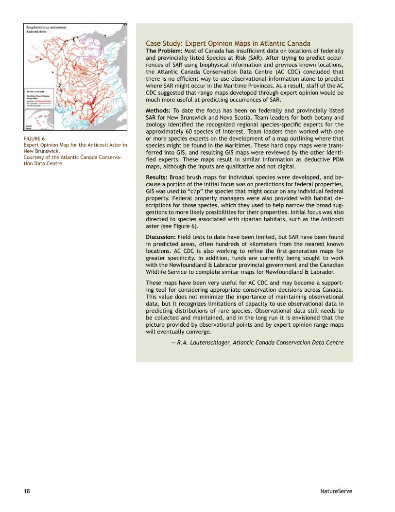
Results: Broad brush maps for individual species were developed, and be-cause a portion of the initial focus was on predictions for federal properties, GIS was used to “clip” the species that might occur on any individual federal property. Federal property managers were also provided with habitat de-scriptions for those species, which they used to help narrow the broad sug-gestions to more likely possibilities for their properties. Initial focus was also directed to species associated with riparian habitats, such as the Anticosti aster (see Figure 6).

Discussion: Field tests to date have been limited, but SAR have been found in predicted areas, often hundreds of kilometers from the nearest known locations.AC CDC is alsoworking to refine the first-generationmaps forgreater specificity. In addition, funds are currently being sought toworkwith the Newfoundland & Labrador provincial government and the Canadian Wildlife Service to complete similar maps for Newfoundland & Labrador.

These maps have been very useful for AC CDC and may become a support-ing tool for considering appropriate conservation decisions across Canada. This value does not minimize the importance of maintaining observational data, but it recognizes limitations of capacity to use observational data in predicting distributions of rare species. Observational data still needs to be collected and maintained, and in the long run it is envisioned that the picture provided by observational points and by expert opinion range maps will eventually converge.

— R.A. Lautenschlager, Atlantic Canada Conservation Data Centre

FIGURE 6 Expert Opinion Map for the Anticosti Aster in New Brunswick. Courtesy of the Atlantic Canada Conserva-tion Data Centre.

Biodiversity Inventory Manual 19

Inventory

Planning

Considerations

Along with identifying species and selecting information sources and inven-tory methods, conducting biodiversity inventories involves careful, up-front consideration of a number of practical issues that may affect both the ability

to conduct an inventory as well as its effectiveness. Several of these considerations are discussed below; others may arise that are more particular to specific inventories or organizations.

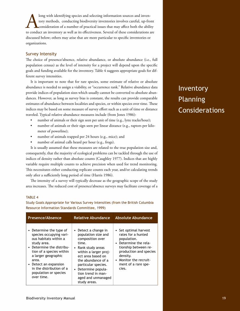
Survey IntensityThe choice of presence/absence, relative abundance, or absolute abundance (i.e., full population census) as the level of intensity for a project will depend upon the specific goals and funding available for the inventory. Table 4 suggests appropriate goals for dif-ferent survey intensities.

It is important to note that for rare species, some estimate of relative or absolute abundance is needed to assign a viability, or “occurrence rank.” Relative abundance data provide indices of population sizes which usually cannot be converted to absolute abun-dances. However, as long as survey bias is constant, the results can provide comparable estimates of abundance between localities and species, or within species over time. These indices may be based on some measure of survey effort such as a unit of time or distance traveled. Typical relative abundance measures include (from Jones 1986):

number of animals or their sign seen per unit of time (e.g., lynx tracks/hour);•number of animals or their sign seen per linear distance (e.g., raptors per kilo-•meter of powerline);number of animals trapped per 24 hours (e.g., mice); and•number of animal calls heard per hour (e.g., frogs).•

It is usually assumed that these measures are related to the true population size and, consequently, that the majority of ecological problems can be tackled through the use of indices of density rather than absolute counts (Caughley 1977). Indices that are highly variable require multiple counts to achieve precision when used for trend monitoring. This necessitates either conducting replicate counts each year, and/or calculating trends only after a sufficiently long period of time (Harris 1986).

The intensity of a survey will typically decrease as the geographic scope of the study area increases. The reduced cost of presence/absence surveys may facilitate coverage of a

Presence/Absence Relative Abundance Absolute Abundance

Determine the type of •species occupying vari-ous habitats within a study area. Determine the distribu-•tion of a species within a larger geographic area.Detect an expansion •in the distribution of a population or species over time.

Detect a change in •population size and composition over time. Rank study areas •within a larger proj-ect area based on the abundance of a particular species.Determine popula-•tion trend in man-aged and unmanaged study areas.

Set optimal harvest •rates for a hunted population.Determine the rela-•tionship between re-production and species density.Monitor the recruit-•ment of a rare spe-cies.

TABLE 4 Study Goals Appropriate for Various Survey Intensities (from the British Columbia Resource Information Standards Committee, 1999)

20 NatureServe

greater geographic area than more intensive methods. In contrast, collecting data to de-termine relative or absolute abundance requires higher levels of funding and expertise. Moreover, more elaborate sampling designs are required to collect abundance data to an adequate level of precision. Absolute abundance data is rarely collected because time and costs are often prohibitive.

Sampling Effort and Statistical RigorIf statistically valid conclusions are necessary (which is uncommon in typical natural heritage inventories), the sampling effort must balance the need to collect sufficient data for valid statistical inferences with the need to minimize cost and cover addition-al ground. Mathematical equations are available to estimate the number of samples required to produce a reliable estimate of a population within a given statistical accuracy.

Where time and budgets allow, more sophisticated monitoring studies may aim to detect changes over time. Statistical estimates of sampling effort required to detect changes or trends rely on the concept of statistical power. The power of a statistical test is influenced by the probability of Type 1 error (e.g. detecting change when none has occurred) and Type 2 error (not detecting change when one has occurred), sample size, population variability, and the strength of the trend (rate of change). Additionally, the relationships between these parameters depend on the ecological process producing the trend and the techniques used to detect it. For this reason, the selection of an appropri-ate study design to evaluate statistical power is critical (Gerrodette 1987).

Co-occurrence of ElementsInventory effectiveness is clearly maximized by targeting sites likely to support mul-tiple elements. The conventional landscape analysis methods described previously, for example, are designed to identify areas likely to support a variety of rare elements or ecological communities in outstanding condition. A similar result may be obtained by overlaying expert opinion maps or element distribution models for multiple species. Of course, simultaneous surveys of rare plants and rare animals require expertise in both disciplines, a combination which tends to be uncommon.

A focus on the co-occurrence of elements is often facilitated by using the coarse-filter approach to inventories. That is, by targeting rare ecological associations or systems, surveyors may be more likely to encounter rare plants, which tend to have strong affini-ties for rare community types.

Seasonality, Phenology, and Determining Presence/Absence As suggested above, depending on the goals of the inventory project, it may be just as important to determine that a species or community type is not present. Such deter-minations are often important in forest management or development projects where habitat alteration is planned. Unfortunately, such “negative data” is usually not recorded with the same rigor as presence data (if at all).

In general, ascertaining presence or absence can be done with confidence only if a number of factors are appropriate: the time of year, time of day, weather conditions, and experience level of observer. An inventory conducted in December that fails to find a rare bog orchid in Minnesota, for example, should not be construed as conclusive evi-dence that the orchid is not there! Recognition of phenologic factors, particularly in the context of the year’s weather patterns (e.g., an early spring), may be critical in identify-ing the appropriate time of survey for certain species groups. Many insects have short

Biodiversity Inventory of Natural Lands 21

flight seasons and may be visible only on sunny days when there is little wind. Some species such as orchids and some wildlife species go through yearly population fluctua-tions and multiple years may be required to definitively determine absence.

In some cases protocols have been developed to definitively determine presence or absence of listed species. For example, the U.S. Fish and Wildlife Service has issued specific trapping protocols for inventories of Preble’s meadow jumping mouse (Zapushudsoniuspreblei): if the protocol is applied for 750 trap-nights without capturing an individual, the USFWS is willing to consider the site “cleared” for the taxon (Beauvais et al 2006). Similar guidelines have been created for field inventories of other listed species.

Urgency It may be prudent to assign higher priorities to sites where management actions or pos-sible changes in ownership are impending. Inventorying and putting effective conserva-tion in place now may provide savings in the long run; it is much more cost-effective to enhance the persistence of a given population before it becomes threatened by manage-ment actions. From the land manager’s perspective, if a plant or animal is likely to be petitioned for protective listing, it is better to address the situation up front and pursue a cooperative conservation agreement. Once a species is listed, it may be more difficult and more expensive to put a management plan in place.

In the context of forest management, it may be most efficient to target sites planned for management activity in the six-month to three-year time frame. In Maine, for ex-ample, close coordination between the Maine Natural Areas Program and corporate landowners has been effective in targeting sites where harvesting was planned within the next two years. If sites are currently being harvested (or where harvesting is imminent), it may be too late to provide useful management guidance through inventory efforts. In geographic terms, forest managers are likely to focus inventory efforts on those elements that may pose operational constraints in forested settings, rather than those that occur on non-forested mountaintops or open bogs. Similarly, sites requiring management ac-tion to promote biodiversity values (invasive species control, use of prescribed fire) may also be high priorities for inventory.

Cost For biodiversity inventories in general, cost effectiveness may be described as the recov-ery of maximum data with minimal effort. For ecological community sampling, cost effectiveness may be defined as the recovery of all vegetation patterns found in an area with the smallest number of samples, smallest sampling crew, and shortest amount of time. Maximizing the cost effectiveness of inventories requires balancing the experience and physical capabilities of individuals, appropriate allocation of time (e.g., working long days when transport to and from the site is involved, whether to have surveyors working individually or in pairs, etc.), and use of efficient sampling techniques and data recording technology (e.g., automated data loggers.)

The cost of collecting data increases as the scale broadens, the focus intensifies, and/or the demand for detailed data increases. For this reason, data collected on a broad scale will likely need to be less comprehensive (i.e., reconnaissance level plots or pres-ence/absence surveys) than data collected on smaller study areas.

In addition, in budgeting for an inventory project it is important to recognize that the accurate mapping, post-processing, and quality control of data (e.g., using Nature-

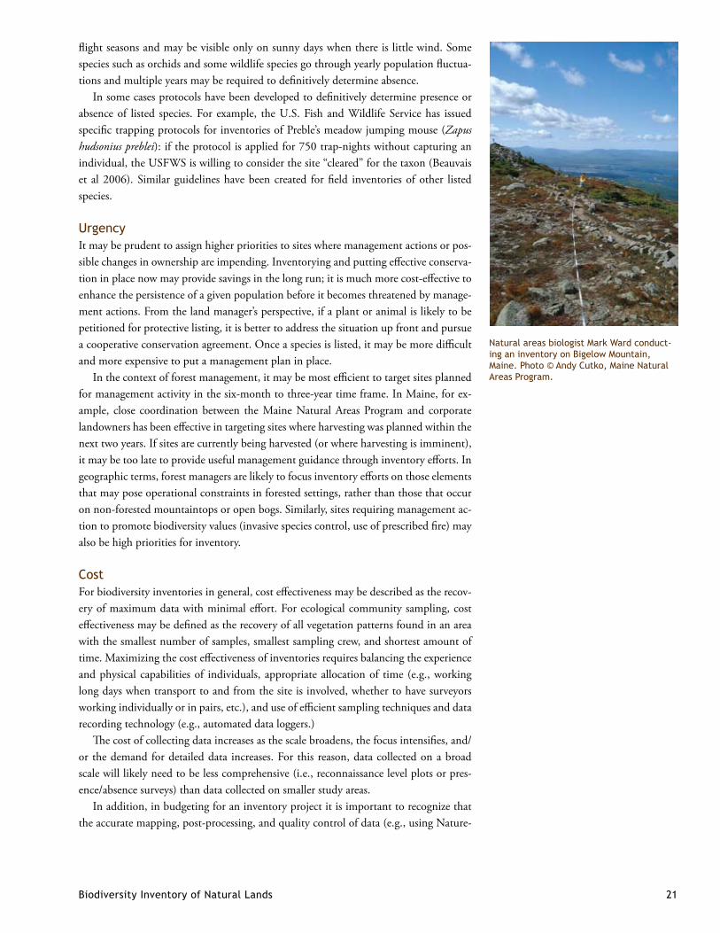
Natural areas biologist Mark Ward conduct-ing an inventory on Bigelow Mountain, Maine. Photo © Andy Cutko, Maine Natural Areas Program.

22 NatureServe

Typical Equipment List for Natural Heritage Inventories

global positioning system (GPS) •hard-copy topographic maps •automated data logger with GIS •capacityair photos and plastic photo •holderfieldnotebook•fieldforms•10x hand lens •tree corer •fieldmanualsforplantorani-•malidentificationnatural community guide or key •pencils •compass •road map •tape measure •colored survey tape (to mark •location or route if necessary) camera equipment •plastic bags for plant or speci-•men collectionwhistle (in case of trouble) •firstaidkit•cell phone and/or walkie-talkies •binoculars •food and water •rain gear•insect repellant •

Serve’s Biotics data management system) often requires as much time per element oc-currence as the field work itself.

Landowner Permission Permission from private landowners (preferably in writing) is required by most natural heritage programs prior to inventory work, and many programs follow up with land-owners about the results of inventory efforts. The landowner permission process adds considerable expense to inventory projects, but in some locations it is a legal require-ment, and it is often an effective initial step in conserving biodiversity. Conversely, lack of landowner permission may significantly inhibit the ability to document biodiversity values across a landscape.

Many state natural heritage programs have formalized the process of landowner con-tact, with landowner tracking databases, form letters, response post cards, and standard-ized text for phone calls.

For More Information: • TheNorthCarolinaNaturalHeritageProgram(2006)hasexamplesoflandownercorrespondencethatreflecttheapproachofmanynaturalheritageprograms.

Opportunity Although biodiversity inventories are often planned through some systematic process focused on geographic regions, species groups, or ecological community types, oppor-tunistic factors such as funding, landowner cooperation, joint projects with other enti-ties, and land protection needs are often a strong influence on inventory priorities. In this regard, an overall strategic plan for inventories (e.g., ecoregional surveys or county surveys) is useful to have in place so that as opportunities arise, they may be quickly evaluated in the context of overall regional inventory priorities.

Accessibility In remote areas, lack of accessibility may be a significant challenge due to lack of roads, steep terrain, water crossings, and other factors. In some cases these challenges may be overcome by adequate funds to cover the extra time or access costs (e.g., helicopter use, back-country equipment). However, because of these extra costs and safety consider-ations, it is not surprising that remote areas tend to have less data coverage than other areas.

In recent years GIS optimization capabilities have enabled remote determination of the most efficient access routes and sampling designs, assessing factors such as road ac-cess, distance, and condition, desired sampling locations, and terrain features.

Safety Safety should always supercede all other factors in conducting inventory work. Many natural heritage programs require teams of two in remote locations to account for safety factors, and researchers working in remote locations should have at least a basic first aid course and communication (cell phone, marine band radio, etc.). Access to habitat types such as cliffs or caves may require additional technical expertise.

Biodiversity Inventory Manual 23

Inventory

and Sampling

Techniques

Species Inventories

There are numerous guides and methods for inventorying and monitoring different species and species guilds, including protocols for sampling design, intensity, and

logistics. For animals, these methods include (to name a few) call-and-response aural surveys, mist netting, point counts, electrofishing, lepidoptera trapping (using mercury vapor lamps or a variety of baits), mark and recapture studies, small mammal trapping (using pitfall or funnel traps, and drift netting), motion-triggered photography and vid-eo surveys, and air surveys of wading birds. For rare plants, inventory techniques include “denovo presence/absence surveys” (a sophisticated way to describe wandering around the woods!), plot-based methods to yield relative abundance, demographic mapping, complete stem counts, and others.

Methods for measuring and monitoring mammals are described well in Wilson et al. (1996), and methods for amphibians are detailed in Donnelly et al. (1994). In addition, many other survey techniques for plants and animals have been perfected by natural heritage staff and remain unpublished. The materials referenced for British Columbia below provide just a few examples of the types of detailed methods used by NatureServe member programs.

For More Information: • TheBritishColumbiaResource Information StandardsCommitteeprovidesinventorymanualsthatdescribedetailedprotocolsforsamplinganddocumentingmorethan30groupsofanimalsandplants.SeeAppendixAforalist.Foranexampleoftheprotocolsforselectedbirdspecies,seetheboxonpage24.

Identification, Verification and Documentation of Specimens For rare specimens, it is often advisable that a voucher specimen is collected and pro-vided to a reputable museum or herbaria (often located at a university). Museums may provide specific guidance on how a specimen is prepared, but at a minimum the col-lection should note the species name and location information (including county, town and specific plant location including lat/long coordinates); habitat and any field charac-teristics that may not be seen on a dried specimen (flower color, habit, tree dimension etc.); date of collection; collector(s); collection number, if used; and who identified the specimen. The decision on whether to collect a specimen should be based on the rarity of the species (with rarer species given high priority) and the population size (collection should not jeopardize the viability of the population). Specimen collection may require obtaining collection permits, especially on land managed by government entities or con-servation organizations or for species that are on federal or state protected lists.

Photographs should be taken if there are only a few plants or as an addition to the specimen. Photos are useful to show natural colors, habit (erect, drooping, clumping etc.), and habitat. A close-up lens can be useful to record small parts of the plant that confirm its identity.

Multiple Species SurveysCertain survey techniques that result in complete species lists for species guilds (e.g., electrofishing, bat netting, numerous insect collection techniques) can be highly efficient because they document multiple elements with limited effort. Multi-species surveys may also enable collection of data on important non-targets (e.g., invasive species, species that are not listed but are in decline). The trade-off is that these efforts often involve the collection and/or identification of numerous common species that may not be of con-servation interest (which can be time consuming, in the case of insects and other taxa). As a result, multiple-species surveys are most useful in conducting de novo inventories where little data exists or for natural community characterization purposes.

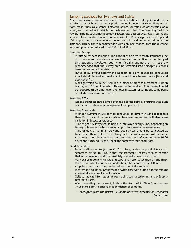
24 NatureServe

Sampling Methods for Swallows and Swifts Point counts involve one observer who remains stationary at a point and counts all birds seen or heard during a predetermined amount of time. Many varia-tions exist, such as distance between points, duration of observation at a point, and the radius in which the birds are recorded. The Breeding Bird Sur-vey,usingpointcountmethodology,successfullydetectsswallowsinsufficientnumbers to allow directional trend analysis. The BBS design has points spaced 800 m apart, with a three-minute count per point and an unlimited detection distance. This design is recommended with only one change, that the distance between points be reduced from 800 m to 400 m. …

Sampling DesignStratifiedrandomsampling:Thehabitatofanareastronglyinfluencesthe•distribution and abundance of swallows and swifts. Due to the clumped distributions of swallows, both when foraging and nesting, it is strongly recommendedthatthesurveyareabestratifiedintohomogenouszonesbased on expected densities. … Hutto et al. (1986) recommend at least 25 point counts be conducted •in a habitat. Individual point counts should only be used once [to avoid duplication] … A design which could be used in a number of areas is a transect 4 km in •length, with 10 point counts of three-minute duration. This transect could be repeated three times over the nesting season (ensuring the same point count stations were not used) …

Sampling EffortRepeat transects three times over the nesting period, ensuring that each •point count station is an independent sample points.

Sampling StandardsWeather: Surveys should only be conducted on days with wind speeds less •than 10 km/hr and no precipitation. Temperature and sun will also cause variation in insect emergence.Time of year: Surveys should begin in late May or early June, depending on •timing of breeding, which can vary up to four weeks between years.Time of day: … to minimize variance, surveys should be conducted at •times when there will be little change in the conspicuousness of the birds. All surveys must be conducted at the same time of day between 10:00 hours and 15:00 hours and under the same weather conditions.

Field ProcedureSelect a direct route (transect) 10 km long or shorter parallel transects •separated by 800 m. Ensure that the transect(s) passes through habitat that is homogenous and that visibility is equal at each point count.Markstartingpointwithflaggingtapeandnoteitslocationonthemap.•Points from which counts are made should be separated by 400 m …All point counts must be conducted outside of the vehicle.•Identify and count all swallows and swifts observed during a three-minute •interval at each point count station. Collect habitat information at each point count station using the Ecosys-•tem Field Form.When repeating the transect, initiate the start point 150 m from the pre-•vious start point to ensure independence of samples.

— excerpted from the British Columbia Resource Information Standards Committee

Biodiversity Inventory of Natural Lands 25

Natural Community and Vegetation Surveys

Natural community inventories may be conducted using a variety of approaches, depending on the project goals. In general, common goals of natural community

sampling include identification of element occurrences (which may be rare natural com-munity types or outstanding examples of common types), sampling to inform natural community classification, wall-to-wall natural community (or ecological system) map-ping, or combinations of all three.

In addition, there are a number of broader ecological objectives that may be ad-dressed by vegetation classification and mapping:

1) To describe vegetation types and establish their regional patterns of distribution; 2) To identify the fundamental relationships of the vegetation types to the physical

factors (e.g., landforms) and ecological processes that act upon them; 3) To analyze the role of natural processes (e.g., fire, windthrow) at regional and

landscape scales on local vegetation structure; and4) To use the identified classification units and processes in characterizing and

evaluating larger landscapes in terms of their vegetation patterns. Both remote and field-based methods are important for natural community surveys.

Factors such as natural community size and landscape context, for example, are often most effectively documented through remote imagery and modified by field visits. See Appendix D for a further discussion of Level 1 (remotely sensed), Level 2 (rapid or ex-tensive evaluation), and Level 3 (intensive measurement and evaluation) methods.

It is important to emphasize that while some ecological inventory work involves quantitative plot-based methods, much of the work carried out by natural heritage pro-grams may be accomplished by qualitative and/or descriptive methods (Levels 1 and 2). Moreover, most natural community classifications do not require quantitative sampling to identify the correct community type.

Some of the common approaches to sampling for natural community mapping and classification purposes are briefly described below.

Qualitative Approaches and Reconnaissance SurveysA considerable amount of natural community inventory work is accomplished through “reconnaissance” level surveys. These surveys involve traversing a site and recording bi-otic and abiotic conditions at various representative reconnaissance points that are doc-umented on field forms (or handheld data recorder) and a GPS. This method consists of qualitative and/or semi-quantitative assessments of features including community type and size, landscape position, vegetation composition and structure, soil characteristics, evidence of past or ongoing disturbance, and landscape context (condition of the sur-rounding lands). In this manner many data points can be recorded in a day, and much more ground may be covered than if quantitative, systematic plots are used. By covering more ground, a surveyor is able to develop a more complete assessment of the associa-tion and ecological system types and their patterns of coverage in a particular area.

For More Information:• Likemanynaturalheritageprograms,theMassachusettsNaturalHeritageandEndangeredSpeciesProgramusesanaturalcommunityfieldformthatincorporatesbothquantitativeandqualitativemethodsforassessingnatu-ralcommunities.Seewww.mass.gov/dfwele/dfw/nhesp/ncforms.pdffordetails.

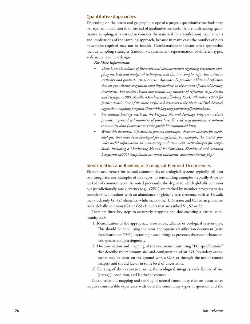
26 NatureServe

Quantitative ApproachesDepending on the intent and geographic scope of a project, quantitative methods may be required in addition to or instead of qualitative methods. Before undertaking quan-titative sampling, it is critical to consider the statistical (or classification) requirements and implications of the sampling approach, because in many cases the number of plots or samples required may not be feasible. Considerations for quantitative approaches include sampling strategies (random vs. systematic), representation of different types, scale issues, and plot design.

For More Information: Thereisanabundanceofliteratureanddocumentationregardingvegetationsam-•plingmethodsandanalyticaltechniques,andthisisacomplextopicbestsuitedtotextbooksandgraduateschoolcourses.AppendixDprovidesadditionalinforma-tiononquantitativevegetationsamplingmethodsinthecontextofnaturalheritageinventories,butreadersshouldalsoconsultanynumberofreferences(e.g.,AustinandHeyligers1989;Mueller-DomboisandEllenberg1974;Whittaker1977)forfurtherdetails.OneofthemoreusefulwebresourcesistheNationalParkService’svegetationmappingprogram(http://biology.usgs.gov/npsveg/fieldmethods).Fornatural heritagemethods, theVirginiaNaturalHeritageProgram’swebsite•providesageneralizedsummaryofproceduresforcollectingquantitativenaturalcommunitydata(www.dcr.virginia.gov/dnh/ncsumproced.htm).Whilethisdocumentisfocusedonforestedlandscapes,therearealsospecificmeth-•odologiesthathavebeendevelopedforrangelands.Forexample,theUSDApro-videsusefulinformationonmonitoringandassessmentmethodologiesforrange-lands,includingaMonitoringManualforGrassland,ShrublandandSavannaEcosystems(2005)(http://usda-ars.nmsu.edu/monit_assess/monitoring.php).

Identification and Ranking of Ecological Element OccurrencesElement occurrences for natural communities or ecological systems typically fall into two categories: any examples of rare types, or outstanding examples (typically A- or B-ranked) of common types. As noted previously, the degree to which globally common but jurisdictionally rare elements (e.g., G5S1) are tracked by member programs varies considerably. Locations with an abundance of globally rare elements, such as Hawaii, may track only G1-G3 elements, while many other U.S. states and Canadian provinces track globally common (G4 or G5) elements that are ranked S1, S2 or S3.

There are three key steps to accurately mapping and documenting a natural com-munity EO:

1) Identification of the appropriate association, alliance or ecological system type. This should be done using the most appropriate classification document (state classification or NVC), factoring in such things as presence/absence of character-istic species and physiognomy.

2) Documentation and mapping of the occurrence unit using “EO specifications” that describe the minimum size and configuration of an EO. Boundary assess-ments may be done on the ground with a GPS or through the use of remote imagery and should factor in some level of uncertainty.

3) Ranking of the occurrence, using the ecological integrity rank factors of size (acreage), condition, and landscape context.

Documentation, mapping and ranking of natural community element occurrences requires considerable experience with both the community types in question and the

Biodiversity Inventory of Natural Lands 27

appropriate mapping and ranking methodologies. For those reasons, identification and ranking are best accomplished by natural heritage staff.

For More Information: • Methodsofdocumentingandrankingspeciesandecologi-calcommunitieshaverecentlybeenrevisedbyNatureServe.SeeChapter4(Occur-renceSpecifications)andChapter5(RankingSpecifications)oftheElementOccur-renceDataStandard(www.natureserve.org/prodServices/eodata.jsp).

Collaboration with Natural Heritage Programs, Data Collection, and Reporting

As the central repository for data on biodiversity features, natural heritage programs play a critical role in evaluating the rarity of species and ecological elements within

a state or provincial context. Moreover, member program staff have unparalleled exper-tise in designing and conducting inventories, evaluating data, and providing the proper statewide or ecoregional context for presenting maps and results. Consequently, it is highly advisable to involve member programs in the planning and implementation of any inventory effort.

When such collaboration is not possible, at a minimum it is important that invento-ry data be shared with member programs. Natural heritage/CDC staff are well qualified to evaluate the accuracy and completeness of data. Furthermore, in some cases direct collaboration with member programs on inventory projects and results may lead to the downlisting of species that were previously thought to be rare.

Field FormsThe most useful guidance on information to gather during species or natural com-munity surveys is provided by natural heritage program rare plant, rare animal, and natural community survey forms. These forms prompt the surveyor with information on population size, condition (e.g., vigor of stems, signs of predation or disease), re-productive status, habitat characteristics, threats, and occurrence ranking. While there is no uniform field form common to all member programs, forms for many programs are quite similar. In many cases these forms are available from the program’s website. In addition, many programs have facilitated data contributions through web portals that use an abbreviated field form.

For More Information: • TheOntarioNaturalHeritageInformationCentre, forexample, solicits informationonspeciesandnaturalcommunities throughanab-breviatedonlinefieldform.Seehttp://nhic.mnr.gov.on.ca/MNR/nhic/communities/comm_report.cfm.Otherexamplesoffieldformsinclude:California:http://www.dfg.ca.gov/whdab/pdfs/natcom.pdfColorado:http://www.cnhp.colostate.edu/documents/field_forms/plant_EOR_digital_ext.pdf

Minnesota:http://nhic.mnr.gov.on.ca/MNR/nhic/communities/comm_report.cfmNevada:http://heritage.nv.gov/comm_w2k.docVermont:http://www.vtfishandwildlife.com/library/forms_and_applications/nongame_and_Natural_Heritage/natural_communities/NaturalCommuni-tyPCform.pdf

28 NatureServe

Automated Data LoggersSome natural heritage programs are now using automated field forms on hand-held data loggers (e.g., IPAQ). When coupled with ARC-PAD or similar mapping software and a GPS, the hand-held data logger provides an integrated field navigation and data col-lection system. The obvious advantage of this system is that it minimizes data transcrip-tion time and errors. The disadvantage is that transcription in the field may be slightly more time consuming than using paper field forms, and any lost data from technical problems may be difficult or impossible to recover.

Mapping Location Data It is highly desirable to document locational information using a global positioning system (GPS), noting the model used and accuracy represented. For linear features or large natural community polygons, multiple GPS points may be needed.

Regardless of the technology used, it is imperative that surveyors record the loca-tional uncertainty of the points or polygons delineated. This uncertainty is critical to accurate mapping and long-term monitoring. Most GPS units provide an estimate of locational uncertainty. The locational uncertainty for larger polygons (a 4,000-acre for-est patch, for example) may relate both to the intensity of the field survey as well as the ability to clearly delineate that stand through remote imagery.

When occurrences are mapped by member programs, there is an important dif-ference between observations, which consist of individual sightings (a mussel found beneath a river bridge, for instance), and an element occurrence, which is a depiction of the larger population of that mussel species (a 2 km reach of that same river). Read-ers should consult with member programs and the latest NatureServe guidance on this topic to ensure that observations and occurrences are being mapped correctly.

For More Information: • AusefuldocumentcontainingdetailsonusingGPSinnatural resource surveys isStandards,SpecificationsandGuidelines forResourceSurveysUsingGlobalPositioningSystem (GPS)Technology, available at http://ilmbwww.gov.bc.ca/bmgs/gsr/specs/index.htm.

nnn

Biodiversity Inventory of Natural Lands 29

Literature Cited

Alvo, R., and S. Ponomarenko. 2003. Vegetation classification standard for Canada workshop: 31 May – 2 June 2000. Canadian Field Naturalist 117(1): 125 –139.

Austin, M.P. and E.M. Adomeit. 1991. Sampling strategies costed by simulation. C.R. Margules and M.P. Austin (editors). Nature conservation: cost effective biological surveys and data analysis, pp. 167 175. Common-wealth Scientific and Industrial Research Or-ganization. Melbourne, Australia.

Austin, M.P., and P.C. Heyligers, P.C. 1989. Vegetation Survey Design for Conserva-tion: Gradsect Sampling of Forests in North-Eastern N.S.W. Biol. Cons. 50. pp. 13-32.

Beauvais, G., D. Kennaith, P. Hernandez, L. Master, and R. Rhurston. 2006. Element Distribution Modeling: A Primer. Unpub-lished manuscript by the Wyoming Natural Diversity Database (WY NDD) and Nature-Serve. Version 2.0. Laramie, WY.

British Columbia Ministry of the Envi-ronment, Resources Inventory Branch. 1998. Species Inventory Fundamentals Standards for Components of British Columbia’s Biodiver-sity; No. 1. 133 pp. Vancouver, B.C.

Brown, D. E. (editor). 1982. Biotic com-munities of the American Southwest-United States and Mexico. Desert Plants 4(1–4):1–342.

Brown, N., L. Master, D. Faber-Langen-doen, P. Comer, K. Maybury, M. Robles, J. Nichols, and B. Wigley. 2004. Managing Ele-ments of Biodiversity in Sustainable Forestry Programs: Status and Utility of NatureServe’s Information to Forest Resources. National Council on Air and Stream Improvement, Technical Bulletin 885.

Buechling, A., and C. Tobalske. 2007. Habitat Modeling of Rare Plant Species in Pa-cific Northwest Forests. A report to the Wey-erhaeuser Foundation by the Oregon Natural Heritage Information Center. Portland, OR.

Caughley, G. 1977. Analysis of Vertebrate Populations. Wiley, London.

Comer, P., D. Faber-Langendoen, R. Ev-ans, S. Gawler, C. Josse, G. Kittel, S. Menard, M. Pyne, M. Reid, K. Schulz, K. Snow, and J. Teague. 2003. Ecological systems in the Unit-ed States: A working classification of terrestrial systems. NatureServe, Arlington, VA.

Corsi, F., J. de Leeuw, and A.K. Skidmore. 2000. Modeling species distribution with GIS. Pages 389-434 in L. Boitani and T.K. Fuller (editors). Research techniques in animal ecolo-gy; controversies and consequences. Columbia University Press, New York, New York, USA.

Cowardin, L. W , V. Carter, F.C. Golet, and E. T. LaRoe. 1979. Classification of wetlands and deepwater habitats of the United States. Biological Service Program, U.S. Fish and W ildlife Service, FWS/OBS 79/31. Department of Interior, Office of Biological Services, Fish and Wildlife Service, Washington, DC.

Cutko, A., and R. Frisina. 2005. Saving All the Parts: A Conservation Vision for Maine Using Ecological Land Units. Maine Depart-ment of Conservation, Augusta, ME.

Dennis, R.L.H., T.G. Shreeve, and H. Van Dyck. 2003. Towards a functional resource-based concept for habitat: a butterfly biology viewpoint. Oikos 102:417-426.

Elith, J., and M.A. Burgman. 2003. Habi-tat models for PVA. Pages 203-235 in C.A. Brigham and M.W. Schwartz (editors). Popu-lation viability in plants: conservation, man-agement and modeling of rare plants. Spring-er-Verlag, New York, New York, USA.

Elith, J., C.H. Graham, R.P. Anderson, M. Dudık, S. Ferrier, A. Guisan, R.J. Hijmans, F. Huettmann, J. Leathwick, A. Lehmann, J. Li, L.G. Lohmann, B.A. Loiselle, G. Manion, C. Moritz, M. Nakamura, Y. Nakazawa, J. McC. Overton, A.T. Peterson, S.J. Phillips, K.S. Richardson, R. Scachetti-Pereira, R.E. Schap-ire, J. Soberon, S. Williams, M.S. Wisz, and N.E. Zimmermann. 2006. Novel methods im-prove prediction of species’ distributions from occurrence data. Ecography 29:129-151.

Eyre, F. H. (editor). 1980. Forest cover types of the United States and Canada. Soci-ety of American Foresters, Washington, DC.

Federal Geographic Data Committee (FGDC). 1997. Vegetation classification stan-dard. FGDCSTD- 005. Vegetation Subcom-mittee, Federal Geographic Data Committee. FGDC Secretariat, U.S.

Ferrier, S., G. Watson, J. Pearce, and M. Drielsma. 2002. Extended statistical ap-proaches to modeling spatial pattern in bio-diversity in northeast New South Wales I: species-level modeling. Biodiversity and Con-servation 11:2275-2307.

Forest Stewardship Council (FSC). 1999. Principle 9 of the FSC Principles and Criteria. Oaxaca, Mexico.

Gauch, H. G., Jr., and R. H. Whittaker. 1981. Hierarchical classification of commu-nity data. Journal of Ecology 69: 135–152.

Gerodette, T. 1987. A power analysis for detecting trends. Ecology 68: 1364-1372.

Gillison, A.N. and K.R.W. Brewer. 1985. The use of gradient directed transects or grad-

30 NatureServe

sects in natural resource survey. Journal of En-vironmental Management. 20:103 127.

Grossman, D.H., D. Faber-Langendoen, A.S. Weakley, M. Anderson, P . Bourgeron, R. Crawford, K. Goodin, S. Landaal, K. Met-zler, K.D. Patterson, M. Pyne, M. Reid, and L. Sneddon. 1998. International classification of ecological communities: Terrestrial vegetation of the United States. Volume I: The vegetation classification standard. The Nature Conservan-cy, Arlington, VA.

Grossman, S. Landaal, K. Metzler, K.D. Patterson, M. Pyne, M. Reid, L. Sneddon, and A.S. Weakley. 1998. International classification of ecological communities terrestrial vegetation of the United States. Volume II: The National Vegetation Classification System: list of types. The Nature Conservancy, Arlington, VA.

Guisan, A. and N.E. Zimmermann. 2000. Predictive habitat distribution models in ecol-ogy. Ecological Modeling 135: 147-186.

Harris, R.B. 1986. Reliability of trend lines obtained from variable counts. Journal of Wildlife Management. 50(1):167-171.

Helman, C. 1983. Inventory analysis of southern New South Wales rainforest vegeta-tion. M.S. thesis. University of New England.

IUCN. 1 996. IUCN Red List of Threat-ened Animals. IUCN, Gland, Switzerland.

Jenkins, R.E. 1985. The identification, ac-quisition, and preservation of land as a species conservation strategy. In: R.J. Hoage, ed. Ani-mal extinctions. Smithsonian Institution Press, Washington, DC.

Jennings, M., O. Loucks, D. Glenn-Lewin, R. Peet, D. Faber-Langendoen, D. Gross-man, A. Damman, M. Barbour, R. Pfister, M. Walker, S. Talbot, J. Walker, G. Hartshorn, G. Waggoner, M. Abrams, A. Hill, D. Roberts, and D. Tart. 2003. Guidelines for describing associations and alliances of the U.S. National Vegetation Classification. The Ecological So-ciety of America, Vegetation Classification Panel, Version 3.0 November 2003. 100 pp. (+ Appendices).

Johnson, Chris J. & Gillingham, Michael P. 2004. Mapping Uncertainty: Sensitivity Of Wildlife Habitat Ratings To Expert Opinion. Journal Of Applied Ecology 41(6), 1032-1041.

Jones, K.B. 1986. The Inventory and Mon-itoring Process. Pages 1-10 in A.Y Cooperrider, R.J. Boyd and H.R. Stuart eds. Inventory and Monitoring of Wildlife Habitat. WR208.

Josse, C., G. Navarro, P. Comer, R. Evans, D. Faber-Langendoen, M. Fellows, G. Kittel, S. Menard, M. Pyne, M. Reid, K. Schulz, K. Snow, and J. Teague. 2003. Ecological systems

of Latin America and the Caribbean: A work-ing classification of terrestrial systems. Nature-Serve, Arlington, VA.

Kartesz, J.T. 1999. A synonymized check-list and atlas with biological attributes for the vascular flora of the United States, Canada, and Greenland. First edition. In Kartesz, JT and CA Meacham. Synthesis of the North American flora [computer program ]. Version 1.0. North Carolina Botanical Garden, Chapel Hill, NC.

Keeton, W. T. and W.W. Gould. 1986. Bio-logical science, fourth edition. W. W. Norton and Co., New York.

Kimmins, J.P. 1997. Forest ecology: A foun-dation for sustainable management. Second edition. Prentice Hall, Upper Saddle River.

Krebs, C.J. 1989. Ecological methodology. Harper Collins, New York. 654 pp.

Lindenmayer, D.B. and J.F. Franklin. 2002. Conserving forest biodiversity: A com-prehensive multiscaled approach. Island Press, Washington, DC.

Master, L. L., L. E. Morse, A. S. Weakley, G. A. Hammerson, and D. Faber-Langendoen. 2003. NatureServe conservation status criteria. NatureServe, Arlington, VA.

McPeek, M. A., and T. E. Miller. 1996. Evolutionary biology and community ecology. Ecology 77: 1319–1320.

Mueller-Dombois, D. and H. Ellenberg. 1974. Aims and methods of vegetation ecol-ogy. John Wiley, New York.

National Research Council. 1993. A bio-logical survey for the Nation. National Acad-emy Press, Washington, DC.

NatureServe. 2004. Benchmark data stan-dards. Revised draft in review.

North Carolina Natural Heritage Program, 2006. Guidelines for Biologists Conducting a Natural Heritage Inventory. North Caro-lina Natural Heritage Program Department of Environment and Natural Resources. Unpub-lished document.

Orloci, L. and W. Stanek. 1979. Vegetation survey of the Alaska Highway, Yukon Territory: types and gradients. Vegetation. 41:1 56.

Pearce, J.L., K. Cherry, M. Drielsma, S. Ferrier, and G. Whish. 2001. Incorporating expert opinion and fine-scale vegetation map-ping into statistical models of faunal distribu-tion. Journal of Applied Ecology 38: 412-424.

Peet, R.K., T.R., Wentworth, R.P. Duncan, and P.S. White. 1997. The North Carolina Vegetation Survey Protocol: A Flexible, Mul-tipurpose Method for Recording Vegetation

Composition and Structure. Unpublished manuscript.

Pielou, E. C. 1984. The interpretation of ecological data: A primer on classification and o rdination. Wiley, New York.

Ponomarenko, S. and R. Alvo. 2000. Per-spectives on developing a Canadian classifi-cation of ecological communities. Canadian Forest Service, Science Branch, Information Report ST-X- 18E. Natural Resources Canada, Ottawa.

Rushton, S.P., S.J. Ormerod, and G. Kerby. 2004. New paradigms for modeling species distributions? Journal of Applied Ecology 41: 193-200.

Scott, J.M., P.J. Heglund, M.L. Morrison, J.B. Haufler, M.G. Raphael, W.A. Wall, and F.B. Samson (editors). 2002. Predicting spe-cies occurrences: issues of accuracy and scale. Island Press, Washington, DC.

Stein, B. A. and F. W. Davis. 2000. Dis-covering life in America: Tools and techniques of biodiversity inventory. In: B. A. Stein, L. S. Kutner, and J.S. Adams, eds. Precious heritage: The status of biodiversity in the United States. Oxford University Press, New York.

Vaughan, I.P. and S.J. Ormerod. 2003. Im-proving the quality of distribution models for conservation by addressing shortcomings in the field collection of training data. Conserva-tion Biology 17:1601-1611.

United Nations Educational, Scientific, and Cultural Organization (UNESCO). 1973. International classification and mapping of vegetation. Series 6. Ecology and conservation. United Nations Educational, Scientific and Cultural Organization, Paris.

Whittaker, R. H. 1962. Classification of natural communities. Botanical Review 28:1–239.

Whittaker, R. H. 1977. Gradient analysis of vegetation. Biological Reviews 49: 207–264.

References for Specific Inventory Methods

Braun, C.E., ed. 2005. Techniques for Wildlife Investigations and Management. The Wildlife Society, Bethesda. 974 pp.

Donnelly, A.M., R.W. Heyer, and W.R. Heyer, eds. 1994. Measuring and Monitoring Biodiversity: Standard Methods for Amphib-ians. Smithsonian Books, Washington, DC. 364 pp.

Hill, D., M. Fasham, G. Tucker, M. Shewry, and P. Shaw, eds. 2005. Handbook of Biodiversity Methods: Survey, Evaluation and

Biodiversity Inventory of Natural Lands 31

Monitoring. Cambridge University Press, New York. 588 pp.

Kirk, D.A. 2004. Guidance for Inventory and Monitoring of Species at Risk on Environ-ment Canada Federal Lands. Report prepared for Species at Risk Division, Recovery Science Canadian Wildlife Service Headquarters, En-vironment Canada by Aquila Applied Ecolo-gists, Ontario. 57 pp.

Marshall, S.A ., R.S . Anderson, R .E. Roughley, V . Behan-Pellletier, and H.V . Danks. 1994. Terrestrial Arthropod Biodi-versity: Planning a Study and Recommended Sampling Techniques. Entomological Society of Canada, Supplement to the Bulletin: 26 (1).

Murphy, B.R. and D.W. Willis, eds. 1996. Fisheries Techniques, Second Edition. Ameri-can Fisheries Society, Bethesda. 732 pp.

North Carolina Natural Heritage Program, 2006. Guidelines For Biologists Conducting A Natural Heritage Inventory, Department of Environment and Natural Resources. Raleigh, NC.

Resources Inventory Committee. 1998. Species Inventory Fundamentals, Standards

for Components of British Columbia’s Biodi-versity; No. 1; Version 2. Prepared by Ministry of Environment, Lands and Parks; Resources Inventory Branch for the Terrestrial Ecosys-tems Task Force, Resources Inventory Com-mittee, Province of British Columbia, Victoria. 119 pp.

Resources Inventory Committee. 1998. Live Animal Capture and Handling Guide-lines for Wild Mammals, Birds, Amphibians & Reptiles, Standards for Components of Brit-ish Columbia ’s Biodiversity; No. 3 ; Version 2 . Prepared by Ministry of Environment, Lands and Parks; Resources Inventory Branch for the Terrestrial Ecosystems Task Force, Resources Inventory Committee, Province of British Co-lumbia, Victoria. 48 pp.

Resources Inventory Committee. 1999. Voucher Specimen Collection, Preparation, Identification & Storage Protocol, Standards for Components of British Columbia’s Biodi-versity; No. 4a; Version 2. Prepared by Min-istry of Environment, Lands and Parks; Re-sources Inventory Branch for the Terrestrial Ecosystems Task Force, Resources Inventory Committee, Province of British Columbia, Victoria. 47 pp.

alliance: A physiognomically uniform group of plant associations sharing one or more dominant or diagnostic species, which as a rule are found in the uppermost stratum of the vegetation (see Grossman et al. 1998; for more recent proposed definitions see Jennings et al. 2003). Dominant species are often emphasized in the absence of detailed floristic information (such as quantitative plot data), whereas other diagnostic species (including characteristic species, dominant differential, and constant species groups) are used where detailed floristic data are available.

association: The finest level of the vegeta-tion classification hierarchy, as well as the basic unit for application of the International Vegetation Classification (IVC). It is defined as “a plant community of definite floristic composition, uniform habitat conditions, and uniform physiognomy” (see Flahault and Schröter 1910, in Grossman et al. 1998; for more recent proposed definitions see Jennings et al. 2003).

biological diversity or biodiversity: The va-riety and abundance of life forms, processes, functions, and structures of plants, animals and other living organisms, including the relative complexity of species, communities,

gene pools and ecosystems at spatial scales that range from local to regional to global.

coarse-filter/fine-filter approach: An ecosys-tem-based approach in which the conserva-tion of multiple, highly functional examples of all characteristic ecosystem types should account for the major ecological patterns and processes at work on the landscape and should adequately provide for habitat requirements of most common and charac-teristic species (“coarse-filter”), and in which a shorter list of vulnerable species assemblages or individual vulnerable species may then provide a practical “fine-filter” focus.

conservation status rank: A measure of the relative risk of extinction for an element at the global level (i.e., range-wide), or the risk of extirpation at the national or subnational level, based on a 1–5 scale. See Table 1, and www.natureserve.org/explorer/ranking.htm.

critically imperiled (G1): See Table 1.

de novo inventories: Ecological surveys of areas not previously inventoried or for species not previously surveyed.

ecological community or natural commu-nity: An assemblage of species that co-occur in defined areas at certain times and have the potential to interact with one another.

Glossary

Resources Inventory Committee. 1999. Voucher Specimen Collection, Preparation, Identification and Storage Protocol, Plants & Fungi, Standards for Components of British Columbia's Biodiversity; No. 4b; Version 2. Prepared by Ministry of Environment,

Lands and Parks; Resources Inventory Branch for the Terrestrial Ecosystems Task Force, Resources Inventory Committee, Prov-ince of British Columbia, Victoria. 37 pp.

United States Department of Interior, Na-tional Biological Survey and National Park Service. 1994. Final Draft Field Methods for Vegetation Mapping NBS/NPS Vegetation Mapping Program. Washington, DC.

Wilson, D .E, F .R. Cole , J.D . Nichols, R . Rudran, and M.S. Foster, eds. 1996. Mea-suring and Monitoring Biological Diversity: Standard Methods for Mammals. Smithsonian Books, Washington, DC. 480 pp.

U.S. Fish and Wildlife Service, Patuxent Wildlife Reearch Center: On-line guide on monitoring birds through point count meth-ods; http://www.pwrc.usgs.gov/bbs/.

32 NatureServe

Ecological communities are often formally classified into types based on vegetation criteria. See association and alliance.

ecological integrity (of communities and systems): The maintenance of structure, spe-cies composition, and the rate of ecological processes and functions within the bounds of normal disturbance regimes (Lindenmayer and Franklin 2002).

ecological system: Groups of plant commu-nities and sparsely vegetated habitats unified by similar ecological processes (e.g., fire, riv-erine flooding), substrates (e.g., shallow soils, serpentine geology), and/or environmental gradients (e.g., local climate, hydrology in coastal zones). They are explicitly defined by spatial and temporal criteria that influence the grouping of communities and habitats. The ecological system will typically manifest itself in a landscape as a spatial aggregation at an intermediate scale (10–100,000 hectares), persisting for at least 50–100 or more years. These and other considerations are intended to ensure that ecological systems form rela-tively robust, cohesive, and distinguishable units on the ground that can serve as practi-cal conservation targets.

element: A biodiversity unit of conservation attention and action for which a conserva-tion status rank is assigned. Elements may be recognized at any taxonomic level, although typically they are only recognized at the species level and below for organisms and the ecological system, alliance, and associa-tion levels for communities. Elements may also be recognized for biodiversity units for which there is no systematic hierarchy (e.g., animal assemblages, community complexes). Elements of conservation concern serve as the targets of natural heritage inventory and mapping. Typically, these targets include native, regularly occurring, vulnerable species (including infraspecific taxa and populations) and exemplary ecological communities and ecological systems.

element occurrence (EO): The spatial representation of a species or ecological com-munity at a specific location. An EO should have practical conservation value for the ele-ment as evidenced by potential continued (or historical) presence and/or regular recurrence at a given location. For species elements, the EO often corresponds with the local population, but, when appropriate, may be a portion of a population (e.g., long-distance dispersers) or a group of nearby populations. For community elements, the EO may repre-sent a stand or patch of a natural community, an ecological system, or a cluster of stands or patches of a natural community. Element occurrences may consist of principal EOs and

sub-EOs. For a full discussion, see http://www.natureserve.org/prodServices/eodata.jsp.

forest certification: A systematic and docu-mented verification process to objectively determine whether a program participant conforms to a particular set of sustainable forestry standards. See the Sustainable For-estry Initiative (SFI, at www.sfi.program.org), Forest Stewardship Council (FSC, at www.fsc.org), and the Canadian Standards Associa-tion (CSA, at www.csa.ca) for details.

formation: Vegetation types that share a defi-nite physiognomy or structure within broadly defined environmental factors, relative landscape positions, or hydrologic regimes. Structural factors such as crown shape and life form of the dominant stratum are used in addition to the physiognomic characters already specified at the higher levels. Hydro-logic modifiers, adapted from Cowardin et al. (1979), are used for wetlands.

imperiled (G2): See Table 1.

locational uncertainty: The recorded location of an observation of an element may vary from its true location due to many factors, including the level of expertise of the data collector, differences in survey techniques and equipment used, and the amount and type of information obtained. This inaccuracy is characterized as locational uncertainty, and is assessed for source features based on the uncertainty associated with the underlying information on the location of the observa-tion.

member programs: Members of the Nature-Serve network, generally known in the U.S. as natural heritage programs and in Canada as conservation data centres.

natural community: See ecologicalcommu-nity.

NatureServe Explorer: A public website (www.natureserve.org/explorer) that provides authoritative conservation information in a searchable database for the plants, animals, and ecological communities of the United States and Canada.

observation: A record that describes a sighting or historical account of a species, community, or ecological system. An obser-vation record on its own does not meet the minimum criteria established for defining an element occurrence, but with the accumula-tion of additional data it may eventually form the basis for an element occurrence.

occurrence rank: Also known as the “ecologi-cal integrity” or “viability” rank, this rank is an approximation of the vigor, health and persistence of a species or natural community. Occurrence ranks include A-D, E (extant), H

(historic), and X (extirpated). The SFI stan-dard refers to protection of “viable” examples of G1 and G2 species, which include all A- and B-ranked occurrences. C-ranked occur-rences are treated on a case-by-case basis, and E-ranked occurrences are considered viable until further information proves otherwise. For a full discussion, see www.natureserve.org/explorer/popviability.htm.

physiognomy: The outward appearance or structure of the vegetation. The upper levels of the International Vegetation Classifica-tion framework are a modification of the UNESCO World Physiognomic Classification of Vegetation (1973) that has been applied worldwide for a variety of natural resource and conservation purposes. Physiognomic levels in the IVC include formation class, for-mation subclass, formation group, formation subgroup, and formation.

species: A genetically distinct group of natural populations that share a common gene pool and that are reproductively isolated from all other such groups (Keeton and Gould 1986). The species’ name is a binomial, consisting of the genus (which groups an organism together with others based on shared traits) and the specific epithet (which denotes the species’ uniqueness from others) (Stein et al. 2000).

vulnerable (G3): See Table 1.

www.natureserve.org