BIOE 293Quantitative

ecology seminarMarm Kilpatrick

Steve MunchSpring Quarter 2015

Seminar Goal

For 5-10 quantitative methods:• To understand how the approach works by reading a

“methods” paper or book chapter on it. This includes the assumptions, strengths, weaknesses, and limitations.

• Read papers more critically. Assess whether an approach is potentially useful for your own work

• Try analyzing data using the approach and discuss challenges.

• Sadly, you likely won’t be an expert in any of the topics at the end, but you’ll have a start at becoming one

Potential Topics & Voting scheme!• 0. Generic intro stuff

• Statistical approaches• Maximum Entropy

• I. Linear models and apps

• Generalized linear models

• Path analysis/SEM• Correlated data• Phylogenetic methods

• II. Linear, multivariate• PCA, MCA, CCA

• III. Multi-layer models• Hierarchical models• Multi-state mark recapture

• IV. Nonlinear from linear

• GAMs• Wavelets

• V. Potpourri• Meta-analyses• Isotope mixing models• Ecological Niche models• Kriging• Machine learning • Occupancy modeling

Statistical approaches

• Frequentist, AIC, Bayesian – what questions are they answering, what advantages/disadvantages do each them have?

• Frequentist: P-values• AIC: Best fitting model(s)• Bayesian: Descriptions of posterior distributions

• Maximum Entropy (a different way of thinking about the same stuff, with different pros/cons)

p(x) is probability density; m(x) is “background probability distribution”

Most statistical methods start with a model for the probability of data (x) given parameters (q)

P(x|q)

a.k.a. the ‘Likelihood’

It’s what happens next that gets people so worked up:

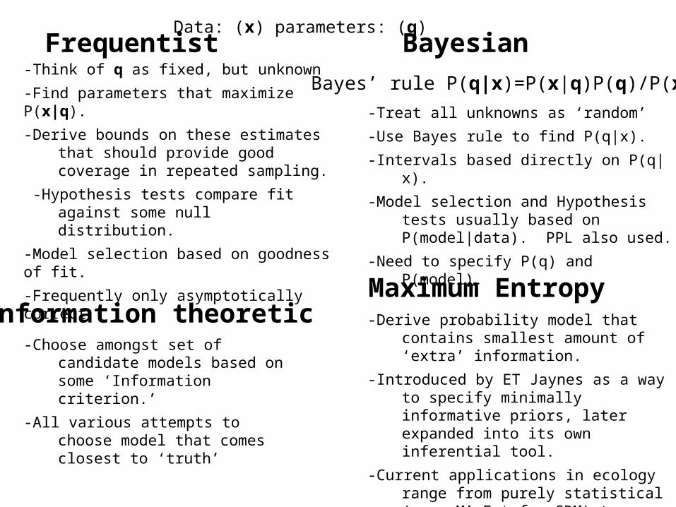
Frequentist Bayesian

Information theoreticMaximum Entropy

-Think of q as fixed, but unknown

-Find parameters that maximize P(x|q).

-Derive bounds on these estimates that should provide good coverage in repeated sampling.

-Hypothesis tests compare fit against some null distribution.

-Model selection based on goodness of fit.

-Frequently only asymptotically correct

-Treat all unknowns as ‘random’

-Use Bayes rule to find P(q|x).

-Intervals based directly on P(q|x).

-Model selection and Hypothesis tests usually based on P(model|data). PPL also used.

-Need to specify P(q) and P(model).

-Choose amongst set of candidate models based on some ‘Information criterion.’

-All various attempts to choose model that comes closest to ‘truth’

-Derive probability model that contains smallest amount of ‘extra’ information.

-Introduced by ET Jaynes as a way to specify minimally informative priors, later expanded into its own inferential tool.

-Current applications in ecology range from purely statistical (e.g. MAxEnt for SDM) to purely theoretical (Harte’s applications to size, area, density distributions)

Bayes’ rule P(q|x)=P(x|q)P(q)/P(x)

Data: (x) parameters: (q)

Linear Models and applications• Generalized linear models and data

transformations: distributions, links, leverage and more

• Correlated data – GLS for time series, spatial data

1940 1960 1980 2000

12

34

5#

mos

q. s

peci

es

NY

1940 1960 1980 2000

23

45

# m

osq.

spe

cies

NJ

1940 1960 1980 2000

1.5

2.0

2.5

3.0

3.5

# m

osq.

spe

cies

CA

Mosquitoes Temp. DDT Population Precip.

1940 1960 1980 2000

0.0

0.2

0.4

0.6

0.8

abun

danc

e

NY

68

1012

14T

emp

Pre

cip

0.0

1.0

2.0

DD

TP

op.

1940 1960 1980 2000

0.0

0.2

0.4

0.6

abun

danc

e

NJ

810

1214

Tem

pP

reci

p

0.0

1.0

2.0

DD

TP

op.

1940 1960 1980 2000

0.0

1.0

2.0

3.0

abun

danc

eCA

46

810

1214

Tem

pP

reci

p

0.0

1.0

2.0

DD

TP

op.

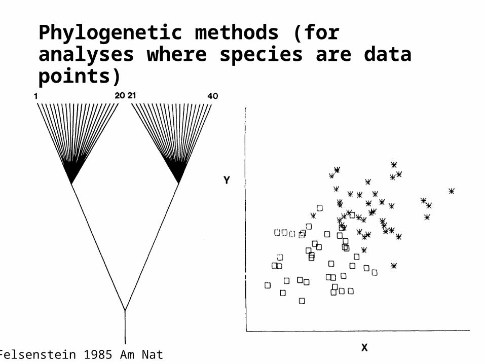
Phylogenetic methods (for analyses where species are data points)

Felsenstein 1985 Am Nat

Linear Models and applications• Path analysis/Structural equation modeling

Hypotheses The data Wootton 1994 Ecology

Multivariate correlational approaches• Principal components analysis (PCA), MCA (PCA

for categorical data), CCA (for exploring correlations between 2 sets of predictors (matrices))

• What people often do after they’ve collected lots of data but don’t know what to do with it

III. Multi-layer models (usually linear, but not necessarily)

• Hierarchical models (Mixed effects models, nested models, random effects models)

• For analyzing data that is influenced by variables that differ at more than one “level”

• Multi-state mark recapture models• Survival analyses• Allow for temporary emigration (temporary movement

to unvisited locations)• Allow for variable states/traits of individuals to

influence survival

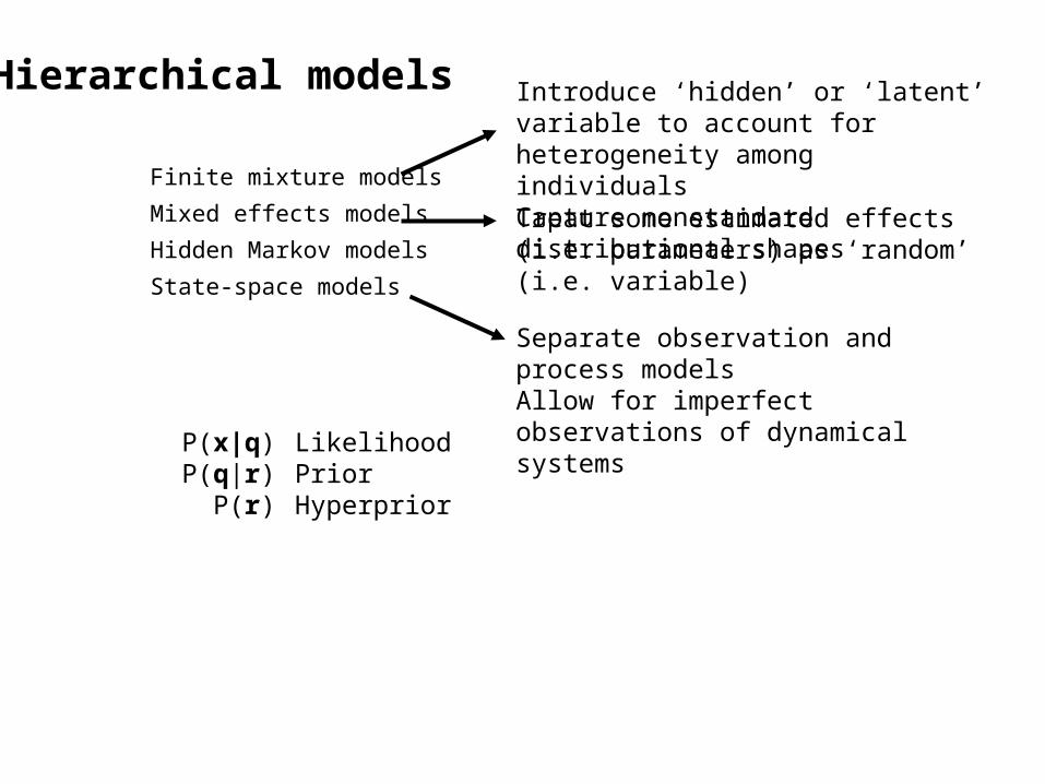
Hierarchical models

Finite mixture models

Mixed effects models

Hidden Markov models

State-space models

P(x|q)P(q|r)

P(r)

LikelihoodPriorHyperprior

Introduce ‘hidden’ or ‘latent’ variable to account for heterogeneity among individuals Capture nonstandard distributional shapes

Treat some estimated effects (i.e. parameters) as ‘random’ (i.e. variable)

Separate observation and process modelsAllow for imperfect observations of dynamical systems

Ecological Niche Models

Occurrence data Environmental variables Probability of occurrence

(Because everyone loves maps)

IV. Nonlinear models (out of linear ones)• Generalized additive models (GAMs)

j

jj xhaxf )()(

Where each f is represented as a ‘basis expansion’

hj(x) are fixed ‘basis functions’and aj are coefficients to be estimated.

Has same structure as a linear model

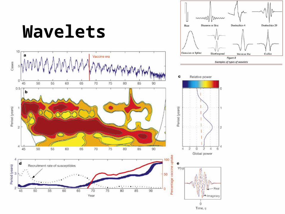
Wavelets

Potpourri(Other topics)

Meta-analyses

Assessing bias, modeling heterogeneity

A method for combining results from multiple studies

Salkeld et al 2013 Ecol Lett

Isotope mixing models

• Estimate the proportions of different food items in your diet

Kriging

Machine learning approaches – regression trees, random forests

• Regression tree: split data into successive groups• Random forests: Lots of regression trees to

minimize overfitting

De’ath&Fabricius 2000 Ecology

Occupancy modeling

• Measuring the occupancy and distribution of an organism when accounting for imperfect detection

• With additional assumptions, can be used to estimate abundance

• Uses repeated visitation of locations and presence/absence of species of interest