Bioecology and Spatial Distribution of the Pistachio

J. Agr. Sci. Tech. (2022) Vol. 24(1): 107-122

107

Bioecology and Spatial Distribution of the Pistachio

Leafhopper, Idiocerus stali Fieber

(Hemiptera: Cicadellidae) in Pistachio Orchards

A. Jamshidi1*

, H. A. Vahedi1, A. A. Zamani

1, and B. Farhadi Bansooleh

2

ABSTRACT

Worldwide, Iran is the first producer of pistachio, which is one of the most

economically important agricultural products for this country. Idiocerus stali Fieber

(Hemiptera: Cicadellidae) is one of the most important pests of this plant. Adults and

nymphs pest feed on leaf tissues and fruit clusters, and they cause damage by sucking the

sap. This pest has one generation per year. In this research, population fluctuations of the

pistachio leafhopper associated to the temperature and humidity changes and its spatial

distribution, using both statistical and geostatistical methods were studied in 2018-2019.

The spatial distribution of all life stages in both years was cumulative according to Iwao

model, whereas considering Taylor's power law model it was cumulative in 2018 and

random in 2019. Considering coefficients' values, both models of Taylor's power law (R2=

0.93) and Iwao model (R2= 0.92) are appropriate for estimating the type of spatial

distribution for this pest, however, Taylor model showed a better data fitting. Concerning

geostatistics models, Kriging interpolation method was more accurate than Inverse

Distance Weighting (IDW) and it was used to produce pest distribution maps. The

movement process of adults, nymphs, and the sites of laying areas per week was precisely

determined. Hence, contamination foci can be identified and used to apply appropriate

management methods at the right time at a low cost.

Keywords: Geostatistics, IPM, Iwao model, Kriging, Taylor's power law.

_____________________________________________________________________________ 1 Department of Plant Protection, College of Agriculture, Razi University, Kermanshah, Islamic Republic

of Iran. 2 Department of Water Engineering, College of Agriculture, Razi University, Kermanshah, Islamic

Republic of Iran.

*Corresponding author; e-mail: [email protected]

INTRODUCTION

Pistachio (Pistacia vera L.,

Anacardiaceae) is one of the indigenous

products in Iran with the highest export and

economic value (Abrishami, 1994).

Currently, Iran is the first largest pistachio

producer with 551307 tons per year (FAO,

2018). The pistachio leafhopper, Idiocerus

stali Fieber (Hemiptera: Cicadellidae) is one

of the important pests of pistachio trees

which reduces pistachio production by

feeding on the sap, making the tree weak

and susceptible to attack by other pests and

diseases.

Adult overwintering leafhopper are the

same color as pistachio tree bark and

females lay one or two eggs after the growth

of tree buds, under the bark of petiole or the

tail of cluster. This species has four nymphal

instars and one generation per year, and 70-

100 eggs per adult are laid (Zenouzi, 1958).

Another study was conducted on I. stali

biology in Qazvin Province. The results

indicated that the emergence of

overwintering adults occurred from the

second week of April, and hatching begins

[ D

OR

: 20.

1001

.1.1

6807

073.

2022

.24.

1.7.

7 ]

[ D

ownl

oade

d fr

om ja

st.m

odar

es.a

c.ir

on

2022

-01-

26 ]

1 / 16

https://dorl.net/dor/20.1001.1.16807073.2022.24.1.7.7

https://jast.modares.ac.ir/article-23-42924-en.html

______________________________________________________________________ Jamshidi et al.

108

in the third week of April. The emergence of

nymphs occurred since mid-May and the

emergence of new generation leafhopper

since mid-June. The average damage to each

cluster was 79.1% (Jalilvand and

Kashanizadeh, 2013).

In Greece, it was reported that high

populations of the pistachio leafhopper

cause the burning of young clusters and

atrophy of leaves (Mourikis et al., 1998).

Another study conducted on pistachio

pests in Turkey stated that overwintering

adults of I. stali were observed from the first

week of March until the buds were opened,

especially on sunny days. Nymphs appeared

from the second week of May, and they

increased in number until the end of May.

Adult appeared on the first week of June

(Yanik and Yucel, 2001).

Due to the significance of this pest on

pistachio trees and the fact that very little

information about this pest is presently

available, it is essential to study its different

biological and ecological aspects. In this

research, field biology and population

fluctuations as well as the spatial

distribution pattern of pistachio leafhopper

were investigated using classical and

geostatistical methods.

MATERIALS AND METHODS

This research was done in the 18-hectare

pistachio garden of the Faculty of

Agriculture, Razi University of Kermanshah

(34˚ 19’ 30.24’’ N - 47˚ 05’ 55.71’’ E and

1,200 meters above sea level) from 2018 to

2019. The distance between trees was five

meters. Sampling of leafhopper population

was investigated from 4 March to 4

November in 2018 and from 3 March to 3

November in 2019. To investigate pistachio

leafhopper's life cycle, 60 branches about 20

cm long containing several leafhopper's eggs

were selected and enclosed by a net and

checked every day, and the life span of the

pest was recorded.

To investigate the population fluctuations

of pistachio leafhopper, different pest life

stages were regularly sampled every week.

In 2018, 50 pistachio trees were selected

with a regular arrangement in five rows out

of 10. One branch was selected on each tree

at two heights of 1.5, and 2.5 m above the

ground in four main directions, and its tip

(the last 20 cm) was carefully examined, and

the number of eggs, nymphs, and adults

were counted and recorded. All four

branches in the four major geographical

directions at every elevation were

considered as a single sampling unit. The

selected 20 cm shoots were marked, and the

same shoots were examined weekly. In

2019, 50 pistachio trees were randomly

selected: on each tree, four 20 cm long

branches were marked, and the number of

eggs, nymphs, and adults were counted and

recorded.

Geographical coordinates (latitude and

longitude due to UTM) of 50 trees selected

in 2018 and 2019 were provided using GPS

for drawing Kriging and IDW maps. The

extracted information was prepared as an

Excel file to be able to transfer to ArcGIS

software after measuring the pest density

and determining the location's geographical

coordinates.

Taylor and Iwao's regressions were used to

determine the pest's spatial distribution

pattern at different life stages.

Regarding Taylor power law, there is a

relation between the population variance

(S2 and he a e age a i n den i ( .

S2 = a

b (1)

To convert the above equation to a linear

relationship and calculate the coefficients (a)

and (b), the sides of Equation (1) are

multiplied by logarithm, and the following

equation is obtained:

Log (s2) = log(a)+b log( ) (2)

Where, a: Width from an origin, which

depends on sample size, and b: The line

slope is an indicator of population

distribution type.

The values smaller, equal, and larger than

the slope of the line show, respectively,

uniform, random, and cumulative

distributions (Arlando and Torres, 2005).

[ D

OR

: 20.

1001

.1.1

6807

073.

2022

.24.

1.7.

7 ]

[ D

ownl

oade

d fr

om ja

st.m

odar

es.a

c.ir

on

2022

-01-

26 ]

2 / 16



Bioecology of Idiocerus stali Fieber ____________________________________________

109

Iwao index is a regression relationship

between Lloyd's mean cr ding ( and

he ean f he a i n ( ca c a ed a

the following equation.

+ m* = (3)

m* = + ( ) – 1 (4)

In he e eq a i n , α e e en he

population's tendency to accumulate (if

positive) or repulsion among individuals (if

nega i e , and β e e en a i n

distribution type. Significant differences

between regression line slope shaving b= 1

(Ta and β= 1 (I a inde e e

calculated with statistic t, equation (5) is

Obtained.

slopeSE

slopet

1 (5)

The value of the calculated t was

compared with t value on the tables

according to the degrees of freedom (n-2). If

the magnitude of the value of calculated t is

larger than t in the table, the difference

between Taylor and Iwao indices will be

important, and the spatial distribution of pest

will be cumulative. If the difference with the

number one is not important, the distribution

is random type (Feng and Nowierski, 1992).

The semi-variogram is used to describe the

spatial relationship of a regionalized variable

(e.g. population density of a pest) at

different locations. The semi-variogram ()

equation is as follows:

)(

1

2)]()([)(2

1)(

hN

i ii hxzxzhN

h

(6)

In this equation, z (xi) is a measured

sample point at xi, z (xi + h) is a measured

sample at point x+h, and N(h) is the number

of pairs separated by lag h. Each calculated

value of semi- variogram along with their

value h indicates a point in the coordinates

of h. The experimental semi- variogram

is obtained by fitting a model to these points

(Madani, 1994).

The ratio DD (Degree of Dependence)=

is a value used to classify the spatial

dependence of variables, where, is nugget

and c is partial sill. If this ratio is less than

25%, the spatial dependence of variable is

weak, whereas if it is from 25 to 75%, its

spatial dependence is moderate, and if it is

greater than 75%, its spatial dependence is

strong (Isaaks and Srivastava, 1989).

All models provided by the software were

used to calculate variograms. In variogram

analysis, the model type and values of

nugget, range, and partial sill were

determined. The ordinary Kriging method

was used for spatial interpolation and

Location map (12 lags were selected; the

amount of lag size at each sampling date

was different due to the different numbers of

insects per date). Kriging is a moving

average weight, that is an interpolation

technique of a variable in non-sampled areas

utilizing variable values at adjacent points

and weights determined by variogram model

(λi (Web e and O i e , 2000 .

= (7)

In this equation is the value estimated

at point , Z(xi) is the actual value of sample

at points xi, n the number of observations

which are in the neighborhood of the point

we want to estimate, andλi is the statistical

weight to sample Z(xi) adjacent to point

assigned.

IDW method is one of the interpolation

methods in which points close to a measured

point are given more weight than points

farther away. Unlike kriging, this method

does not follow the assumptions about the

spatial relation among data (no variogram).

It solely relies on the assumption that points

closer to estimation point are more similar to

farther points. In this study, an IDW with a

power 2 was chosen (Webster and Oliver,

2000).

The cross-validation method was used to

evaluate the efficiency of interpolation

methods. The Root Mean Square Error

[ D

OR

: 20.

1001

.1.1

6807

073.

2022

.24.

1.7.

7 ]

[ D

ownl

oade

d fr

om ja

st.m

odar

es.a

c.ir

on

2022

-01-

26 ]

3 / 16



______________________________________________________________________ Jamshidi et al.

110

(RMSE) was considered for assessment

models. Finally, population density maps of

different life stages of pistachio leafhopper

were drawn by using ArcGIS 10.6 version.

RESULTS

Field Biology of Idiocerus stali

This pest is overwintering as an adult, under

the bark and fissure of pistachio trees.

Overwintering adults were gray in color, and

in early March, with the warming of the

weather, left overwintering places and started

walking on the branches of pistachio trees.

They fed standing on buds, dropping sap. The

first egg laid was observed in late March.

Females create holes using their ovipositor in

petioles, fruit tails, or cluster tails, and in each

hole, one or two eggs were placed diagonally.

Then, the eggs were covered with secretions

that became black during the time, and laying

locations were identifiable as black dots. The

eggs were oval, milky in color and 0.8±0.07

mm in length (30 eggs were measured with a

ruler below the binocular). The average laying

period was two and a half months. Embryonic

development took from 15 to 20 days. Four

nymphal ages were observed. After hatching,

the first nymphs appeared, and they fed on

fruits, tail clusters, and petioles, and by

producing honeydew, making clusters and

leaves sticky. When they had completed their

growing period, they went back to leaves and

molted. The second instar nymphs appeared in

late April, third instar nymphs emerged in

early May, and the fourth instar nymphs

appeared in late May, and like the first

nymphs, fed on tail clusters and petioles and

they molted in the lower page of leaves. The

growth period of pistachio nymphs was 60

days on average, and the duration of the first,

second, third, and fourth instar were

7.48±0.11, 12.22±0.24, 12.43±0.21 and

12.62±0.12 days, respectively. After the last

molt, adult summer forms appeared in the late

May, and then they moved to overwintering

places.

Population Fluctuations of Idiocerus

stali

In 2018, the first instar nymphs peaked on 20

May with a mean population of 12.16±1.82

{mean per sampling unit [all four branches (the

last 20 cm) in four major geographical directions

in every elevation on each tree were considered

as a single sampling unit]± standard error} and

the second instar nymphs reached their peak with

an average population of 17.26±2.04 on 27 May

(Figure 1). The peak of the third instar nymphs

with a mean population of 25.74±3.5 was on 3

June, and the fourth nymphs with a mean

population of 14.88±1.58 reached their peak

on10 June. Egg peak date was 22 April, with a

mean population of 64.04±17.58 and adults

reached a peak on 1 July with a mean population

of 22.86± 1.6.

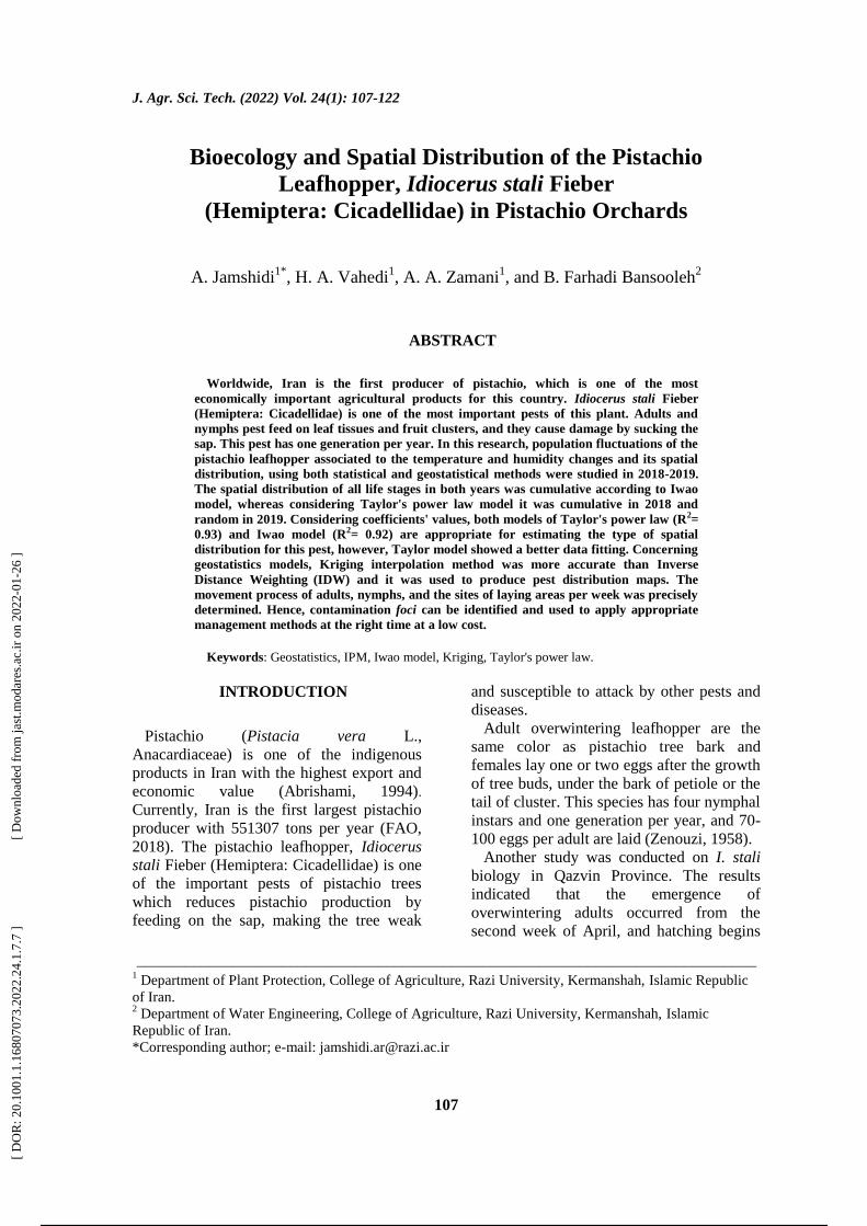
In 2019, population peaks for nymphs from the

first to the fourth instar were 9.52±1.71,

16.62±1.7, 23.22±3.27, and 9.58±1.57,

respectively, and occurred on 26 May, 2, 9, and

16 Jun, respectively. Eggs reached their peak on

28 April with mean population of 26.1±4.64, and

adults on 7 July with a mean population of

20.28±1.9. (Figure 2)

Relationship between Temperature and

Humidity with Population Fluctuation

In 2018, there was an important

relationship between temperature changes

and the adult population fluctuation, which

was a direct relation (Figure 1). There was no

important relationship among the population

fluctuations of the other life stages and whole

immature I. stali and temperature changes.

There was an important direct relation among

humidity changes and egg population

fluctuations, 1st instar, 2

nd instar, and whole

immature stages. There was an important and

inverse relation among humidity changes and

adults population fluctuations. Population

fluctuations in nymphs with age three and

four had no important relation with humidity

changes.

In 2019, there was an important relation and

inverse between temperature changes

[ D

OR

: 20.

1001

.1.1

6807

073.

2022

.24.

1.7.

7 ]

[ D

ownl

oade

d fr

om ja

st.m

odar

es.a

c.ir

on

2022

-01-

26 ]

4 / 16




111

Figure 1.The curve of average population fluctuations of total life stages Idiocerus stali and the average temperature and

humidity during different days of sampling in 2018.

[ D

OR

: 20.

1001

.1.1

6807

073.

2022

.24.

1.7.

7 ]

[ D

ownl

oade

d fr

om ja

st.m

odar

es.a

c.ir

on

2022

-01-

26 ]

5 / 16



______________________________________________________________________ Jamshidi et al.

112

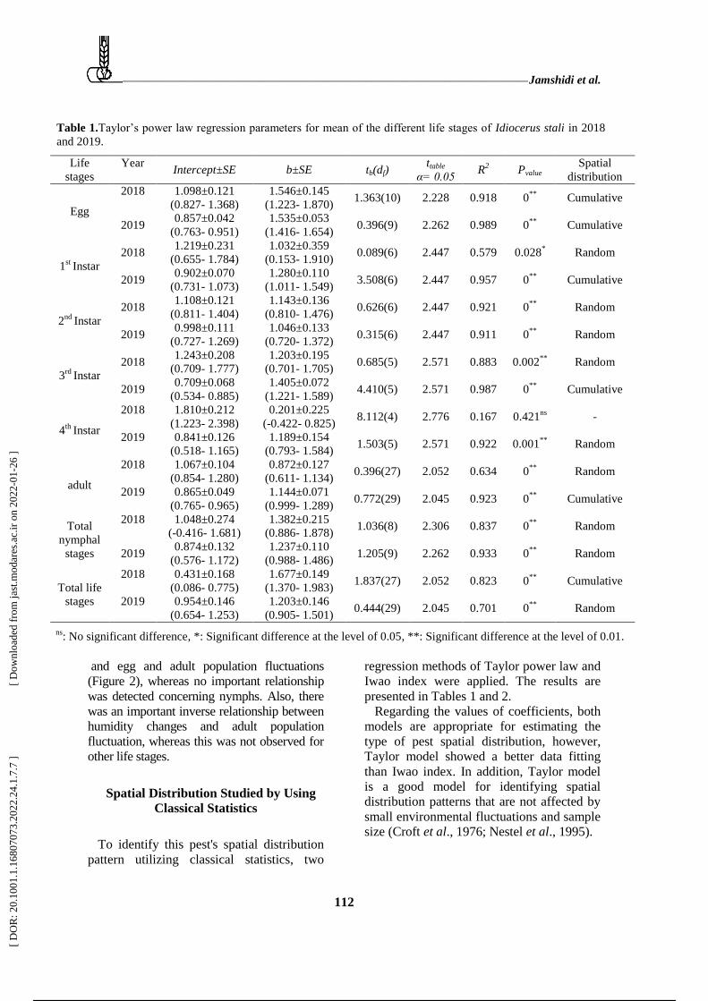
Table 1.Ta ’ e a eg e i n a a e e f ean f he diffe en ife age f Idiocerus stali in 2018

and 2019.

Spatial

distribution Pvalue R

2 ttable

α= 0.05 tb(df) b±SE

Intercept±SE

Year Life

stages

Cumulative 0**

0.918 2.228 1.363(10) 1.546±0.145

(1.223- 1.870)

1.098±0.121

(0.827- 1.368)

2018

Egg

Cumulative 0**

0.989 2.262 0.396(9) 1.535±0.053

(1.416- 1.654)

0.857±0.042

(0.763- 0.951) 2019

Random 0.028* 0.579 2.447 0.089(6)

1.032±0.359

(0.153- 1.910)

1.219±0.231

(0.655- 1.784) 2018

1st

Instar

Cumulative 0**

0.957 2.447 3.508(6) 1.280±0.110

(1.011- 1.549)

0.902±0.070

(0.731- 1.073) 2019

Random 0**

0.921 2.447 0.626(6) 1.143±0.136

(0.810- 1.476)

1.108±0.121

(0.811- 1.404) 2018

2nd

Instar

Random 0**

0.911 2.447 0.315(6) 1.046±0.133

(0.720- 1.372)

0.998±0.111

(0.727- 1.269) 2019

Random 0.002**

0.883 2.571 0.685(5) 1.203±0.195

(0.701- 1.705)

1.243±0.208

(0.709- 1.777) 2018

3rd

Instar

Cumulative 0**

0.987 2.571 4.410(5) 1.405±0.072

(1.221- 1.589)

0.709±0.068

(0.534- 0.885) 2019

- 0.421ns

0.167 2.776 8.112(4) 0.201±0.225

(-0.422- 0.825)

1.810±0.212

(1.223- 2.398)

2018

4th

Instar

Random 0.001**

0.922 2.571 1.503(5) 1.189±0.154

(0.793- 1.584)

0.841±0.126

(0.518- 1.165)

2019

Random 0**

0.634 2.052 0.396(27) 0.872±0.127

(0.611- 1.134)

1.067±0.104

(0.854- 1.280)

2018

adult

Cumulative 0**

0.923 2.045 0.772(29) 1.144±0.071

(0.999- 1.289)

0.865±0.049

(0.765- 0.965)

2019

Random 0**

0.837 2.306 1.036(8) 1.382±0.215

(0.886- 1.878)

1.048±0.274

(-0.416- 1.681)

2018 Total

nymphal

stages Random 0**

0.933 2.262 1.205(9) 1.237±0.110

(0.988- 1.486)

0.874±0.132

(0.576- 1.172) 2019

Cumulative 0**

0.823 2.052 1.837(27) 1.677±0.149

(1.370- 1.983)

0.431±0.168

(0.086- 0.775)

2018

Total life

stages Random 0

** 0.701 2.045 0.444(29)

1.203±0.146

(0.905- 1.501)

0.954±0.146

(0.654- 1.253)

2019

ns: No significant difference, *: Significant difference at the level of 0.05, **: Significant difference at the level of 0.01.

and egg and adult population fluctuations

(Figure 2), whereas no important relationship

was detected concerning nymphs. Also, there

was an important inverse relationship between

humidity changes and adult population

fluctuation, whereas this was not observed for

other life stages.

Spatial Distribution Studied by Using

Classical Statistics

To identify this pest's spatial distribution

pattern utilizing classical statistics, two

regression methods of Taylor power law and

Iwao index were applied. The results are

presented in Tables 1 and 2.

Regarding the values of coefficients, both

models are appropriate for estimating the

type of pest spatial distribution, however,

Taylor model showed a better data fitting

than Iwao index. In addition, Taylor model

is a good model for identifying spatial

distribution patterns that are not affected by

small environmental fluctuations and sample

size (Croft et al., 1976; Nestel et al., 1995).

[ D

OR

: 20.

1001

.1.1

6807

073.

2022

.24.

1.7.

7 ]

[ D

ownl

oade

d fr

om ja

st.m

odar

es.a

c.ir

on

2022

-01-

26 ]

6 / 16




113

Table 2. I a ’ eg e i n a a e e f ean f he diffe en ife age f Idiocerus stali in 2018 and 2019.

Spatial

distribution Pvalue R

2 ttable

α=

0.05

tb(df) ±Seβ ±SEα

Year Life

stages

Cumulative 0**

0.995 2.228 0.605(10) 4.639±0.110

(4.415- 4.864)

7.990±1.924

(3.702- 12.278)

2018

Egg

Cumulative 0**

0.930 2.262 0.396(9) 2.407±0.220

(1.910- 2.904)

6.886±2.416

(1.419- 12.352)

2019

- 0.895

ns 0.003 2.447 0.046(6) -0.415±3.012

(-7.784- 6.953)

29.837±17.803

(-13.725-

73.398)

2018

1stInstar

Random 0.002

**

0.824 2.447 0.293(6) 1.686±0.317

(0.910- 2.462)

7.805±1.658

(3.748- 11.862)

2019

- 0.134

ns 0.333 2.447 0.013(6) 1.164±0.672

(-0.480- 2.808)

15.904±7.045

(1.333- 33.142)

2018

2nd

Instar

Random 0.010

**

0.694 2.447 0.006(6) 0.976±0.264

(0.329- 1.622)

10.407±2.412

(4.506- 16.309)

2019

- 0.203

ns 0.300 2.571 0.021(5) 1.445±0.987

(-1.092- 3.981)

25.296±15.170

(-13.700-

64.292)

2018

3rd

Instar

Cumulative 0**

0.982 2.571 0.318(5) 1.678±0.101

(1.420- 1.937)

4.130±1.338

(0.692- 7.568)

2019

- 0.655

ns 0.054 2.776 0.436(4) -0.149±0.309

(-1.006- 0.708)

22.099±3.011

(13.738-

30.460)

2018

4th

Instar

Random 0.007

**

0.793 2.571 0.095(5) 1.278±0.292

(0.528- 2.028)

7.067±2.319

(1.107- 13.027)

2019

- 0.274

ns 0.044 2.052 0.044(27) 0.470±0.421

(-0.394- 1.334)

15.945±4.102

(7.529- 24.362)

2018

adult

Random 0**

0.711 2.045 0.035(29) 1.144±0.135

(0.867- 1.420)

7.059±1.015

(4.983- 9.136)

2019

Random 0.008

** 0.605 2.306 0.020(8) 1.609±0.459

(0.551- 2.667)

26.679±14.723

(-7.273- 60.631)

2018 Total

nymphal

stages Random 0**

0.926 2.262 0.021(9) 1.143±0.107

(0.900- 1.386)

11.032±3.057

(4.118- 17.947)

2019

Cumulative 0**

0.698 2.052 0.051(27) 2.984±0.377

(2.210- 3.759)

-8.419±10.226

(-29.401-

12.564)

2018

Total life

stages

Cumulative 0**

0.815 2.045 0.026(29) 1.281±0.113

(1.049- 1.512)

9.606±2.575

(4.340- 14.873)

2019

ns: No significant difference, *: Significant difference at the level of 0.05, **: Significant difference at the level of 0.01.

Spatial Distribution Studied by Using

Geostatistics Methods

To select the most appropriate

interpolation method, the best semi-

variogram function should be selected to

fit the data. The results for all life stages

of leafhopper are presented in Table 3 for

2018 and in Table 4 for 2019. For each

sampling date, the best semi-variogram

model of all models offered by ArcGIS is

identified, and its associated geostatistical

description was provided. After selecting

the appropriate semi-variogram functions,

Kriging interpolation methods and IDW

tested the RMSE of these two methods

[ D

OR

: 20.

1001

.1.1

6807

073.

2022

.24.

1.7.

7 ]

[ D

ownl

oade

d fr

om ja

st.m

odar

es.a

c.ir

on

2022

-01-

26 ]

7 / 16



______________________________________________________________________ Jamshidi et al.

114

Figure 2. The curve of average population fluctuations of total life stages Idiocerus stali and the average temperature and

humidity during different days of sampling in 2019.

[ D

OR

: 20.

1001

.1.1

6807

073.

2022

.24.

1.7.

7 ]

[ D

ownl

oade

d fr

om ja

st.m

odar

es.a

c.ir

on

2022

-01-

26 ]

8 / 16




115

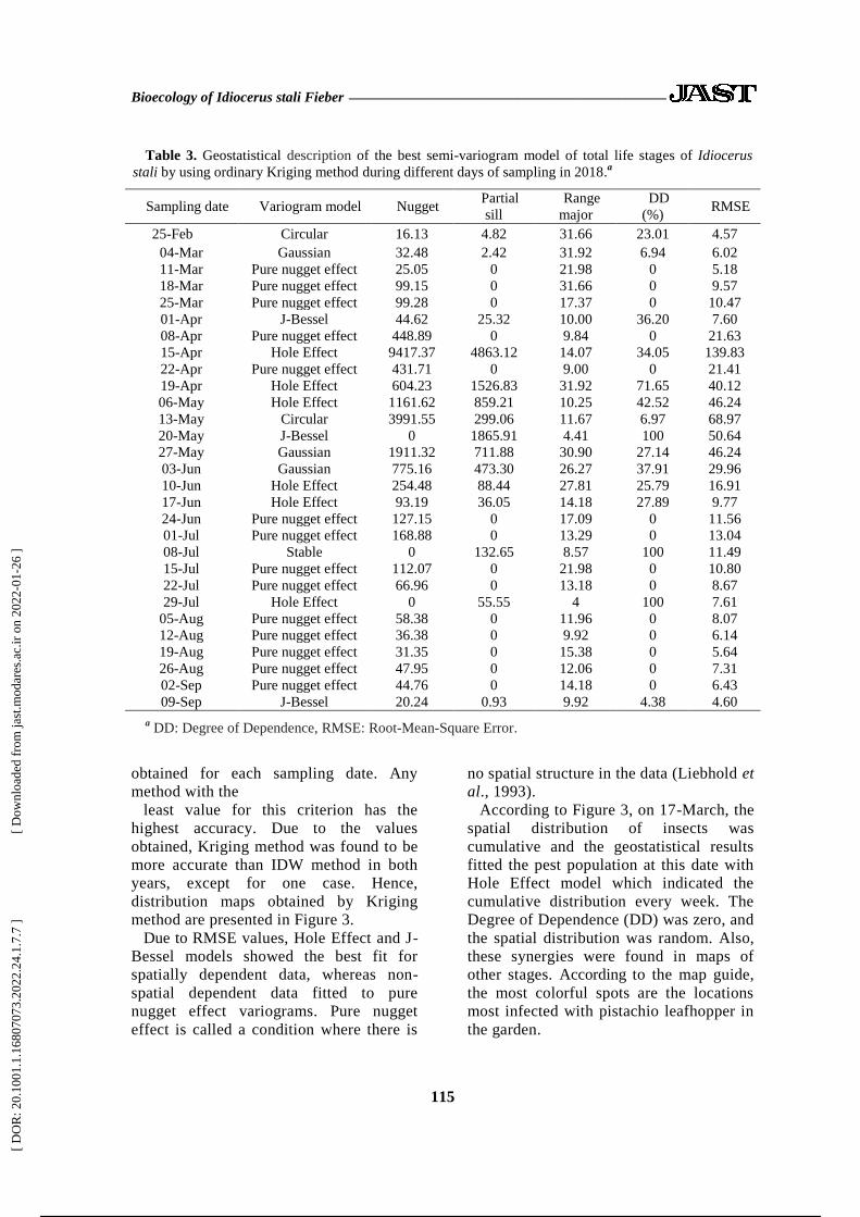
Table 3. Geostatistical description of the best semi-variogram model of total life stages of Idiocerus

stali by using ordinary Kriging method during different days of sampling in 2018.a

Sampling date Variogram model Nugget Partial

sill

Range

major

DD

(%) RMSE

25-Feb Circular 16.13 4.82 31.66 23.01 4.57

04-Mar Gaussian 32.48 2.42 31.92 6.94 6.02

11-Mar Pure nugget effect 25.05 0 21.98 0 5.18



01-Apr J-Bessel 44.62 25.32 10.00 36.20 7.60

08-Apr Pure nugget effect 448.89 0 9.84 0 21.63

15-Apr Hole Effect 9417.37 4863.12 14.07 34.05 139.83


19-Apr Hole Effect 604.23 1526.83 31.92 71.65 40.12

06-May Hole Effect 1161.62 859.21 10.25 42.52 46.24

13-May Circular 3991.55 299.06 11.67 6.97 68.97

20-May J-Bessel 0 1865.91 4.41 100 50.64

27-May Gaussian 1911.32 711.88 30.90 27.14 46.24

03-Jun Gaussian 775.16 473.30 26.27 37.91 29.96

10-Jun Hole Effect 254.48 88.44 27.81 25.79 16.91

17-Jun Hole Effect 93.19 36.05 14.18 27.89 9.77

24-Jun Pure nugget effect 127.15 0 17.09 0 11.56

01-Jul Pure nugget effect 168.88 0 13.29 0 13.04

08-Jul Stable 0 132.65 8.57 100 11.49



29-Jul Hole Effect 0 55.55 4 100 7.61

05-Aug Pure nugget effect 58.38 0 11.96 0 8.07




02-Sep Pure nugget effect 44.76 0 14.18 0 6.43

09-Sep J-Bessel 20.24 0.93 9.92 4.38 4.60

a DD: Degree of Dependence, RMSE: Root-Mean-Square Error.

obtained for each sampling date. Any

method with the

least value for this criterion has the

highest accuracy. Due to the values

obtained, Kriging method was found to be

more accurate than IDW method in both

years, except for one case. Hence,

distribution maps obtained by Kriging

method are presented in Figure 3.

Due to RMSE values, Hole Effect and J-

Bessel models showed the best fit for

spatially dependent data, whereas non-

spatial dependent data fitted to pure

nugget effect variograms. Pure nugget

effect is called a condition where there is

no spatial structure in the data (Liebhold et

al., 1993).

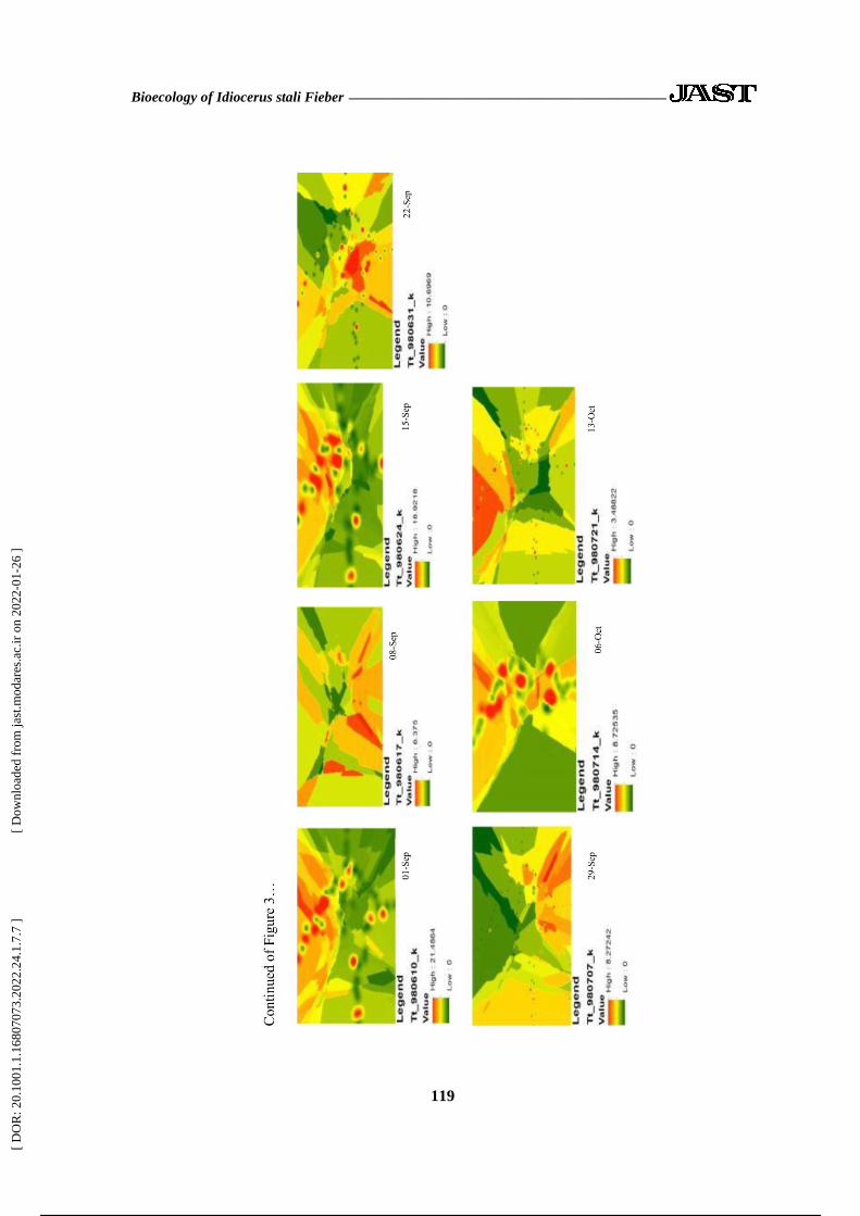
According to Figure 3, on 17-March, the

spatial distribution of insects was

cumulative and the geostatistical results

fitted the pest population at this date with

Hole Effect model which indicated the

cumulative distribution every week. The

Degree of Dependence (DD) was zero, and

the spatial distribution was random. Also,

these synergies were found in maps of

other stages. According to the map guide,

the most colorful spots are the locations

most infected with pistachio leafhopper in

the garden.

[ D

OR

: 20.

1001

.1.1

6807

073.

2022

.24.

1.7.

7 ]

[ D

ownl

oade

d fr

om ja

st.m

odar

es.a

c.ir

on

2022

-01-

26 ]

9 / 16



______________________________________________________________________ Jamshidi et al.

116

Table 4.Geostatistical description of the best semi-variogram model of total life stages of Idiocerus stali

by using ordinary Kriging method during different days of sampling in 2019.a

Sampling date Variogram model Nugget Partial sill Range major DD (%) RMSE

17-Mar Hole Effect 10.74 0.04 95.88 0.39 3.14



07-Apr J-Bessel 0 105.67 0.02 100 9.51


21-Apr Circular 1145.91 8.86 74.00 0.77 33.41


05-May Pure nugget effect 470.67 0 164.39 0 22.09



26-May J-Bessel 0 930.97 21.25 100 31.35

02-Jun Pure nugget effect 729.24 0 155.93 0 27.16

09-Jun Hole Effect 684.98 464.94 55.04 40.43 32.01

16-Jun Gaussian 1074.68 98.92 246.97 8.43 30.01

23-Jun Gaussian 205.76 84.17 210.75 29.03 15.39

30-Jun J-Bessel 157.97 35.82 55.04 18.49 13.03



21-Jul Gaussian 83.29 1.86 237.99 2.19 9.73

28-Jul J-Bessel 21.98 38.95 24.78 63.92 8.19

04-Aug Pentaspherical 54.72 1.33 64.16 2.37 7.72

11-Aug Gaussian 39.62 12.34 210.75 23.75 6.65


25-Aug K-Bessel 21.76 1.11 64.49 4.86 4.82

01-Sep Hole Effect 4.18 25.46 24.39 85.89 5.35

08-Sep J-Bessel 14.99 20.57 20.05 57.84 5.85




06-Oct Pure nugget effect 4.69 0 115.97 0 2.12

13-Oct Pure nugget effect 0.77 0 246.97 0 0.92

a DD: Degree of Dependence, RMSE: Root-Mean-Square Error.

DISCUSSION

In this research, four nymphal instars were

observed for I. stali, which is in accord with

Jalilvand and Kashanizadeh (2013). Zenouzi

(1958) also stated four nymphal instars,

whereas in another research three nymphal

instars were observed (Behdad, 1984).The

reason for this difference can be attributed to

weather conditions or differences in

nutrition quality.

In Behdad's (1984) studies, the life stage

duration of the first, second, and third instar

were from 7 to 9 days, from 10 to 15 days,

and from 12 to 15 days, respectively, which

corresponds to the times recorded in the

present study.

The average population of different life

stages of this pest was higher in 2018 than in

2019: this can be attributed to the

application of pesticides in 2019 (Confidor®

0.4 per thousand), which reduced pest

population. No spraying was done in the

study area in 2018. Moreover, the

emergence of overwintering adults started

two weeks earlier in 2018 (4 March, against

17 March in 2019). The reason for this

difference might be high rainfall in March

[ D

OR

: 20.

1001

.1.1

6807

073.

2022

.24.

1.7.

7 ]

[ D

ownl

oade

d fr

om ja

st.m

odar

es.a

c.ir

on

2022

-01-

26 ]

10 / 16




117

[ D

OR

: 20.

1001

.1.1

6807

073.

2022

.24.

1.7.

7 ]

[ D

ownl

oade

d fr

om ja

st.m

odar

es.a

c.ir

on

2022

-01-

26 ]

11 / 16



______________________________________________________________________ Jamshidi et al.

118

[ D

OR

: 20.

1001

.1.1

6807

073.

2022

.24.

1.7.

7 ]

[ D

ownl

oade

d fr

om ja

st.m

odar

es.a

c.ir

on

2022

-01-

26 ]

12 / 16




119

[ D

OR

: 20.

1001

.1.1

6807

073.

2022

.24.

1.7.

7 ]

[ D

ownl

oade

d fr

om ja

st.m

odar

es.a

c.ir

on

2022

-01-

26 ]

13 / 16



______________________________________________________________________ Jamshidi et al.

120

2019, which caused leafhoppers to leave

their overwintering places later.

According to Yanik and Yucel's (2001)

findings in Birecik region in Turkey,

overwintering adults appeared in garden

during the first week of March, but adults

were also observed in summer form on 1

June, consistent with our findings. The

reason can be the similar weather conditions

in the two regions.

According to the results, the range of

semi-variogram was different from 4 to 247

m and DD (Degree of Dependence) was

from 0 to 100% (Table 3). In geostatistics,

higher range values are more useful in pest

anage en . In a ing he e ’

population, the distance between samples

can be increased up to 75% of the range

value (Hassani Pak, 1997). For example, if

the range value is 100 m, we can collect the

samples at a distance of 75 m from each

other. Therefore, in a region with a specified

area, as the range value increases, fewer

samples are required to estimate the

population density of a pest. In other words,

the range of semi-variogram plays an

important role in determining the distance

between samples.

Iwao index was not important for adults

and all nymphs in 2018, and it could not

detect the spatial distribution of these steps.

In Taylor's power law method, the egg

stage's spatial distribution and the sum of all

life stages were recognized as cumulative,

and the rest of stages as random. In 2019, in

Iwao method, the eggs' spatial distribution,

third instar nymphs, and sum of whole life

stages were recognized cumulative and the

remaining stages as random. In Taylor's

power law method, the spatial distribution of

eggs, the first and third nymphs and adults,

appointed cumulative, and the rest of stages

were random. However, according to

geostatistical methods, the spatial

distributions of all stages were generally

random. However, the spatial distribution

per week was determined precisely.

Geostatistics is one of the most accurate

methods of estimation; it examines many

factors like distance among points,

anisotropy, and spatial variability. An

advantage of geostatistics is a careful survey

for spatial distribution and locations of

different life stages of a pest and

identification of contaminated places.

Different methods of pest control can be

accurately performed at low cost. The results

showed that Kriging method was highly

accurate for estimating population density of

this pest in non-data points.

For better management of pests, predicting

its abundance and population distribution is

very important (Trematerra et al., 2007).

Therefore, it requires careful monitoring,

and that is why spatial analysis methods,

like geostatistics, are widely used in

entomology (Liebhold et al., 1993,

Trematerra and Sciarretta, 2004). Following

the classical statistics, the indices usually

focus on the distribution of sample

abundance and measure the relation of

sample variance with its mean, but they

ignore insects' spatial location, which itself

produces undesirable effects; for example,

these indices usually cannot distinguish

among different spatial patterns (Hurlbert,

1990). Their interpretation of spatial pattern

largely depends on the size of sample units

(Sawyer, 1989). As a result, the methods

depend on samples' geographical location

for investigating their spatial location.

Geostatistical techniques are a good

alternative. Taylor and Iwao indicators can

only provide a distribution coefficient for

the whole season, and the sampling dates

cannot be separated by them (Southwood

and Henderson, 2000).The locations of

whole life stages, laying, and movement of

leafhopper adults and nymphs were

precisely determined each week. Therefore,

it is possible to identify contamination foci

and take over appropriate management

measures in the right time at low cost.

The present study shows the superiority of

geostatistical methods over classical

statistical methods in line with reducing the

pesticide consumption and site specific

integrated pest management. The

geostatistical method shows the places

where the pest has more accumulation, and

[ D

OR

: 20.

1001

.1.1

6807

073.

2022

.24.

1.7.

7 ]

[ D

ownl

oade

d fr

om ja

st.m

odar

es.a

c.ir

on

2022

-01-

26 ]

14 / 16




121

by spraying in that particular place, we can

avoid excessive consumption of pesticides;

as a result, we cause less damage to the

environment.

REFERENCES

1. Abrishami, M. H. 1994. Persian Pistachio, a

Comprehensive History. University

Publication Center, Iran, 669 pp.

2. Arlando, P. S. and Torres, L. M. 2005.

Spatial Distribution and Sampling of

Thaumetopoea pityocampa (Lep.:

Thaumetopoeidae) Populations on Pinus

Pinstar. For. Ecol. Manag.,210: 1-7.

3. Behdad, A. 1984. Pests of Iranian Fruit

Trees. Bina Pub, Isfahan Printed, Iran, 743

pp.

4. Croft, B. A., Welch, S. M. and Dover, M. J.

1976. Dispersion Statistics and Sample Size

Estimates for Populations of the Mite

Species, Panonychus ulmi and Amblyseius

fallacis on Apple. Environ. Entomol., 5(2):

227-233.

5. FAO. 2018. Food and Agricultural

Commodities Production. Available in:

http://www.fao.org/faostat/en/#data/QC.

6. Feng, M. G. and Nowierski, R. M. 1992.

Spatial Distribution and Sampling Plans for

Four Species Cereal Aphid (Hom,:

Aphididae) Infesting Spring Wheat in

Southwestern Idaho. J. Econ. Entomol., 85:

830-837.

7. Hassani Pak, A. A. 1997. Geostatistics

Tehran University Press 314 PP.

8. Hurlbert, S. H. 1990. Spatial Distribution of

the Montane Unicorn. Oikos,58: 257-271.

9. Isaaks, E. H. and Srivastava, R. M. 1989. An

Introduction to Applied Geostatistics.

Oxford University Press,New York USA,

592 PP.

10. Jalilvand, N. and Kashanizadeh, S. 2013.

Study on the Biology of Idiocerus stali

Qazvin Climate. Bull. Agr. Natur. Resour.

Res., 15: 22-30.

11. Liebhold, A. M., Rossi, R. E. and Kemp, W.

P. 1993. Geostatistics and Geographic

Information Systems in Applied Insect

Ecology. Annu. Rev. Entomol., 38: 303-327.

12. Madani, H. 1994. Fundamentals of

Geostatistics. First Edition, Amir Kabir

University of Technology, Tafresh Branch,

Iran, 668 PP.

13. Mourikis, P. A., Sourgianni, A. T. and

Chitzanidis, A. 1998. Pistachio Nut Insect

Pests and Means of Control in Greece. II

International Symposium Pistachio and

Almonds, Acta Hortic., 470: 604-611.

14. Nestel, D., Cohen, H., Saphir, N., Klein, M.

and Mendel, Z. 1995. Spatial Distribution of

Scale Insects: Comparative Study Using

Ta ’ P e La . Environ. Entomol.,

24(3): 506-512.

15. Sawyer, A. J. 1989. Inconstancy of Taylor's

b: Simulated Sampling with Different

Quadrat Sizes and Spatial Distributions. Res.

Popul. Ecol., 31: 11-24.

16. Southwood, T. R. E. and Henderson, P. A.

2000. Ecological Methods. 3rd

Edition

Blackwell Science, Oxford.

17. Trematerra, P., Gentile, P., Brunetti, A.,

Collins, L. E. and Chambers, J. 2007.

Spatio-Temporal Analysis of Trapcatches of

Tribolium confusum du Val in a

Semolinamill, with a Comparison of Female

and Male Distributions. J. Stor. Prod. Res.,

43: 315-322.

18. Trematerra, P. and Sciarretta, A. 2004.

Spatial Distribution of Some Beetles

Infesting a Feed Mill with Spatio-Temporal

Dynamics of Oryzaephiluss urinamensis,

Tribolium castaneum and Tribolium

confusum. J. Stor. Prod. Res., 40: 363-377.

19. Webster, R. and Oliver, M. A. 2000.

Geostatistics for Environmental Scientists.

ISBN: 0-41-96553-7, Wiley Press, 271 PP.

20. Yanik, E. and Yucel, A. 2001. The Pistachio

(P. vera L.) Pests, Their Population

Development and Damage State in Sanliurfa

P ince. In: “XI GREMPA Seminar on

Pistachios and Almonds”, (Ed. : Ak, B. E.,

CIHEAM, Zaragoza, PP. 301-309.

21. Zenouzi, H. 1958. Pistachio Leafhopper and

Way of Its Controling. Iran Agr. Promot.

Org., 34: 14.

[ D

OR

: 20.

1001

.1.1

6807

073.

2022

.24.

1.7.

7 ]

[ D

ownl

oade

d fr

om ja

st.m

odar

es.a

c.ir

on

2022

-01-

26 ]

15 / 16

http://www.fao.org/faostat/en/#data/QC



______________________________________________________________________ Jamshidi et al.

122

:.Idiocerus stali Fieber (Hem فضایی زنجرک پسته، توزیع بیواکولوژی و

Cicadellidae) پسته باغات رد

بانسوله فرهادی ب. و زمانی ع. ا. ، واحدی ح. ا. جمشیدی، .آ

چکیده

یي هحصلات کطبرسی ایزاى هحصلی صبدراتی ارس آر است.تزتزیي اقتصبدیپست اس هن

،Idiocerus stali Fieber (Hem., Cicadellidae) سجزکایزاى الیي تلیذ کذ پست است.

خض ببفت بزگ اس بی ایي سجزکحطزات کبهل پراست. ایي هحصلتزیي آفبت یکی اس هن

. بیاکلصی ایي آفت هطبلع ضذ کذهکیذى ضیز پزرد خسبرت ارد هی بب هی پست تغذی کزد

هطخص ضذ ک یک سل در سبل دارد. در ایي پضص سببت جوعیت سجزک پست در ارتببط بب

تغییزات درج حزارت رطبت هطبلع ضذ. تسیع فضبیی هجوع هزاحل سیستی بز اسبط هذل آیائ در

اس ع تجوعی، اهب در سبل 7931ع تجوعی بد بز اسبط هذل قبى تاى تیلر در سبل ز د سبل اس

= R2) تیلر قذرت قبى هذل هذل د ز ضزایب تبئیي، هقبدیز ب تج اس ع تصبدفی بد. بب 7931

ر در ستذ هذل تیل هبسب آفت فضبیی تسیع ع تخویي بزای (R2 = 0.92) هذل آیائ ( 0.93

کذ. ب را بزاسش هی ب داضت بتز اس ضبخص تیلر دادوبستگی بیطتزی بب داد هقبیس بب هذل آیائ

وچیي پزاکص فضبیی سجزک پست بب استفبد اس سهیي آهبر ن بزرسی ضذ. بز اسبط تبیج رش

تزی داضت قط بی دقت ببلا Inverse Distance Weighting (IDW)کزیجیگ در هقبیس بب رش

بی چیي هحلب نپزاکص آفت بب استفبد اس ایي رش تی ضذ. رذ حزکت حطزات کبهل پر

بی آلدگی را ضبسبیی تاى کبىگذاری در ز فت دقیقب هطخص ضذ ب ایي تزتیب هیتخن

بم داد.اقذاهبت هذیزیتی هبسب را در سهبى هبسب بب شی کن اج

[ D

OR

: 20.

1001

.1.1

6807

073.

2022

.24.

1.7.

7 ]

[ D

ownl

oade

d fr

om ja

st.m

odar

es.a

c.ir

on

2022

-01-

26 ]

Powered by TCPDF (www.tcpdf.org)

16 / 16



http://www.tcpdf.org

Documents

Bioecology and Spatial Distribution of the Pistachio