1

BIOL 434/509: Population genetics

Professor Dr. Michael Whitlock Zoology Department Biodiversity 216 whitlock@zoology.ubc.ca Office Hours: 1:30-2:30 Mondays and after class most days course web-page: http://www.zoology.ubc.ca/~whitlock/bio434/

2

BIOL  434/509:    POPULATION  GENETICS  ........................................................................  1  

WHAT  IS  POPULATION  GENETICS?  ...............................................................................  3  

REVIEW  OF  HARDY-­‐WEINBERG  .....................................................................................  4  

PROBABILITY  REVIEW  ................................................................................................  11  

RANDOM  GENETIC  DRIFT  ...........................................................................................  15  

THE  EFFECTIVE  POPULATION    SIZE  ..............................................................................  26  

MUTATION  ................................................................................................................  39  

SELECTION  .................................................................................................................  47  

INBREEDING  ...............................................................................................................  73  

SEX  RATIO  EVOLUTION  ...............................................................................................  86  

POPULATION  STRUCTURE  ..........................................................................................  88  

INTRODUCTION  TO  QUANTITATIVE  GENETICS  ..........................................................  110  

3

What is Population Genetics? The genetical study of the process of evolution (The study of the change of allele frequencies, genotype frequencies, and phenotype frequencies)

Population Genetics is… • About microevolution (evolution within species) • Strongly dependent on mathematical models (which have been more successful than

most areas of mathematical biology) • A relatively young science (most important discoveries are from after 1930)

Factors causing genotype frequency changes • Selection • Mutation • Random Drift • Migration • Recombination • Non-random Mating

What's the most important factor in evolution? SELECTION Natural selection causes evolution if (1) There is variation in fitness (selection) (2) That variation can be passed from one generation to the next (inheritance) This is the central insight of Darwin.

4

Review of Hardy-Weinberg

Allele Frequency The proportion of all alleles in all individuals in the group in question which are of a particular type. (often referred to as "gene frequency")

e.g. 40 individuals which are AA 47 individuals which are Aa 13 individuals which are aa

GENOTYPE AA Aa aa Total

# of individuals 40 47 13 100 # of A alleles 80 47 0 127 # of a alleles 0 47 26 73

Total # of alleles

200

Allele frequency of A = 127/200 = 0.635 pA=0.635 pa = 73/200 = 0.365 = 1- pA

Genotype Frequency The proportion of individuals in a group with a particular genotype. (Genotype can refer to one locus, two loci, or the whole genome, depending on the context) 40 AA 47 Aa 13 aa = 100 Total individuals pAA = 40/100 = 0.4 pAa = 47/100 = 0.47 paa = 13/100 = 0.13

Hardy-Weinberg Equilibrium How to predict genotype frequencies from allele frequencies • A useful null model • Actually predicts genotype frequencies quite well, quite often

5

Assumptions (1) Organism is diploid (2) Reproduction is sexual (3) Generations are non-overlapping (4) Mating occurs at random (5) Population size is very large (6) Migration is zero (7) Mutation is zero (8) Natural selection does not affect the gene in question

1-locus, 2-alleles pAA + pAa + paa = 1 Frequency of A allele?

€

pA =2pAA + pAa

2

€

pa =2paa + pAa

2

Mating Table – Random union of gametes Assume that all of the H-W conditions are met, and that gametes find each other at random.

Combination Freq. Offspring Frequencies

AA Aa aa A x A pA

2 1 A x a pApa 1 a x A papA 1 a x a pa

2 1 pA

2 2 pApa pa2

6

These are the Hardy-Weinberg frequencies. A (frequency p) a (frequency q=1–p) A

AA (pAA=p2)

Aa (pq)

a

Aa (pq)

aa (q2)

What if individuals (instead of gametes) pair at random? Pair Frequency Offspring

Frequency

AA Aa aa AA x AA pAA

2 1 AA x Aa 2pAApAa 1/2 1/2 AA x aa 2pAApaa 1 Aa x Aa pAa

2 1/4 1/2 1/4 Aa x aa 2pAapaa 1/2 1/2 aa x aa paa

2 1 pA

2 2pApa pa2

Note that we also get the Hardy-Weinberg frequencies, but we didn't specify that the parents were in Hardy-Weinberg.

7

Hardy-Weinberg Principle With the assumptions listed before, the frequencies of AA, Aa, and aa are p2, 2pq, and q2. Note: The allele frequency has not changed: p2 + pq = p (Early Mendelians believed that dominant alleles would sweep through populations without selection -- WRONG!) H-W proportions are necessary, but not sufficient to demonstrate that all of the assumptions are true.

0.2 0.4 0.6 0.8 1

0.2

0.4

0.6

0.8

1Fr

eque

ncy

p

q2 (paa)2pq (pAa)

p2 (pAA)

8

Example: Scarlet Tiger Moth (Panaxia dominula)

1469 white spotted (AA) 138 medium number of spots (AA') 5 few spots (A'A') 1612

€

p =14691612

+121381612" #

$ %

= 0.954

q = 0.046

Expected Frequency x N Observed

p2 = (0.954)2 = 0.9101 1467 1469

2pq = 2 (0.954)(0.046) 142 138 q2

= (0.046)2 = 0.0021 3 5

9

H-W with more than 2 alleles n alleles: A1, A2, A3, A4,… An frequencies: p1, p2, p3, p4,… pn

€

pii=1

n

∑ = 1

Frequency of AiAi homozygote is pi

2 Frequency of AiAj heterozygote is 2pipj Heterozygosity: H=1-Σpi

2

H-W for an X-linked locus

Allele frequency:

€

p =pm3

+2pf3

where pm is the allele frequency in males and pf is the allele frequency of females. Allele frequency change over generations:

€

" p m = pf

" p f =pm + pf

2

So the Hardy-Weinberg equilibrium is NOT reached in one generation for X-linked loci, if pm ≠ pf

10

Genotype frequencies for 2 loci Let pA be the frequency of allele A (so (1-pA) is the frequency of a) at the A locus and pB be the frequency of allele B (so (1-pB) is the frequency of b) at the B locus [Note: pA, pB are used differently in different contexts!] At Hardy-Weinberg equilibrium, the frequency of a 2-locus genotype is the product of the frequencies of the two 1-locus genotypes it contains. i.e. freq(Aabb) = 2pA(1-pA) x (1-pB)2 BUT, with two loci, this equilibrium is not reached immediately (unlike the one locus case) If recombination occurs between the 2 loci at rate r, then the frequency of the AB gamete in the next generation is given by:

€

" P AB = 1− r( )PAB + r pA pB The (1-r)PAB term comes from the non-recombinants, and the r pA pB term comes from the recombinants. So if PAB ≠ pA pB, then the system is not in equilibrium. This is called linkage disequilibrium. This term is a misnomer because it does not require physical linkage and it may have a non-zero value at equilibrium, when selection. migration or another process acts to create associations between alleles. D = PAB Pab - PAb PaB

€

PAB = pA pB + DPAb = pA pb − DPaB = pa pB − DPab = pa pb + D

€

Dt = 1− r( )t D0, where Dt is the linkage disequilibrium at time.

11

Probability Review

Distributions A distribution function describes the probability of any given outcome for some process There are continuous distributions (e.g. normal, χ2, Γ) and discrete distributions (e.g. binomial and Poisson).

Binomial Distribution

P x( ) = nx

!

"#

$

%& px (1− p)n−x

p: probability of a particular event n: number of trials P[x]: probability that the event occurs exactly x times in N trials.

Remember, nx

!

"#

$

%&=

n!n− x( )!x!

For example, the number of alleles of type A in one generation, taken as a sample from the alleles of the previous generation.

Poisson Distribution

P x[ ] = e−µµ x

x!

where e is the base of the natural log, and µ is the expected number of successes per unit time. x! is "x factorial" = x (x-1) (x-2) (x-3) …3 x 2 x 1 Discrete, like the binomial, but the number of trials is undefined e.g., the number of offspring per mother the number of flowers per m2

Normal Distribution

€

f x( ) =12πσ 2

e−x−µ( )2

2σ 2

where µ is the mean of the distribution and σ2 is the variance.

12

Continuous Very common in nature, because of the Central Limit Theorem e.g., distribution of heights or weights, sampling error

Expected Values, Means, Variances The expected value is the sum (or integral) of all possible values of quantity in question times their probabilities. Represented by E[y]

E[x] =

€

x f (x)all x∑ for discrete distributions

13

=

€

x f (x) dx−∞

∞

∫ for continuous distributions

The mean of x is the expected value of x.

µ or

€

x =

€

x f (x)all x∑ or

€

x f (x) dx−∞

∞

∫

The mean measures the central tendency of a distribution.

The variance is the expected value of

€

x − µ( )2

The variance measures the spread of the distribution.

V or σ2 or s2 =

€

E x − µ( )2[ ] =

€

x − µ( )2 f (x)all x∑ or

€

x − µ( )2 f (x) dx−∞

∞

∫

Mean and Variance of basic distributions Mean Variance Binomial pN Np(1-p) Poisson µ µ Normal µ σ2

Useful facts about means and variances Mean Variance

X + Y E[X] + E[Y] V[X] +V[Y] + 2COV[X,Y] -X - E[X] V[X] a X a E[X] a2 V[X]

X + a E[X] + a V[X] COV[X, Y] is the covariance of X and Y

€

Cov[X,Y ] = E x − µx( ) y − µy( )[ ]

14

Conditional Probability The probability that X is true, given that Y is true, is written as P[X | Y]. e.g. The probability that a 20 year-old is in college = 40% The probability that a 60 year-old is in college = 0.5% P[an individual is in college | that individual is 20 years old] = 0.4. We can find the probability of an event, if we know the probability of that event under each of possible scenarios and the probability of those scenarios:

€

P X[ ] = P X |Y[ ]all Y∑ P Y[ ]

e.g. Hardy- Weinberg: What is the probability that an allele drawn from an individual is type A? P[A | Individual is of genotype AA] = 1 P[A | Individual is of genotype Aa] = 1/2 P[A | Individual is of genotype aa] = 0 So P[A] = P[A |AA] P[AA] + P[A |Aa] P[Aa] + P[A |aa] P[aa]

= (1) p2 + (1/2) 2pq + (0) q2 =p2+ pq = p(p + q) = p

P(X and Y) = P(X) P(Y |X) If X and Y are independent, then P(X and Y) =P(X) P(Y) (Relate this to linkage disequilibrium.)

15

Random Genetic Drift Most populations are small enough that, by chance, sampling will result in a different allele frequency from one generation to the next. This is called "Genetic Drift".

16

The two founders of population genetics, Sewall Wright and Ronald Fisher disagreed most strongly about the importance of genetic drift. What happens in an individual population is unpredictable, but we can describe the distribution of allele frequencies among replicate populations.

Sampling Start with an ideal population (= all individuals have an equal probability of being the parent of an individual from the next generation). (We know that these are unreasonable assumptions. We'll fix this later with the idea of an effective population size.) With N individuals (or 2N alleles) With an ideal population, and two different alleles, the number of copies of a particular allele in the next generation follows a binomial distribution

P x( ) = 2Nx

!

"#

$

%& px (1− p)2N−x

Pop 1 Pop 2 Pop 3 Pop 4

...

...

...

Time t

t+1

t+2

.

.

.

(no migration)

17

Digression into the binomial distribution General Population Genetics for diploids n = # of trials 2N = # of alleles X = number of "successes" X = # of A alleles p = probability of success p = allele frequency E[X] = np E[X] = 2Np V[X]=np(1-p) V[X]=2Np(1-p) p' = X/(2N), so…

E[p'] = p

€

= E X2N" # $

% & '

=E[X]2N

=2Np2N

= p( ) *

+ , -

€

V " p [ ] =p 1− p( )2N

= V X2N$ % &

' ( )

=V X[ ]2N( )2

=2Np(1− p)2N( )2

=p 1− p( )2N

*

+ ,

-

. /

€

E " p [ ] = p V " p [ ] =pq2N

So with pure drift… • The expected value of the allele frequency doesn't change. • The amount of drift is inversely proportional to population size.

(For haploids, there are N alleles in the population, so E !p[ ] = p V !p[ ] = pqN

)

Drift over time Random genetic drift can continue until one allele is fixed (i.e. reaches a frequency of 1) or lost (reaches a frequency of 0). Without selection, mutation or migration, eventually every allele will be either fixed or lost. The probability of eventual fixation of an allele affected only by drift = p (its allele frequency) {Think about why.}

18

4 ways to model drift

1. Wright Fisher Model (Transition matrix) With drift, there is some probability that the allele frequency in the next generation could be any value. The binomial distribution gives the probability of drawing a certain number of alleles of a given type from the pool of available parental alleles. The probability of drawing j alleles of a particular type out of 2N, given that there are i alleles of that type in the parental generation (let's call this Tij) is:

€

Tij =2Nj

"

# $

%

& '

i2N" #

% &

j

1− i2N

" #

% &

2N − j

Remember that p is i/2N (and q = 1 – p), so Tij is really a function of p. So if we want to calculate the distribution of allele frequencies after one generation of drift, we can use Tij. This Tij is called a transition probability -- it is the probability of transitioning from i copies of the allele to j copies in one generation.

€

Pr j copies afterone generation[ ] = Tij Pr[icopiesnow]i=0

2N

∑

What if we wanted to know the probability of changing from i copies in one generation to k copies in two generations? Then we use conditional probability. The probability of having a certain number of copies in two generations depends on what happens in the next generation. So

€

P[k copies in 2 generations]

= P[k | j copies in 1 generation]P[ j copiesinonegeneration]j=0

2N

∑

=i=0

2N

∑ Tjk Tij( )j=0

2N

∑ Pr[icopiesat start]

This could be continued for as many generations as desired. Fortunately, this can be eased by noticing that the transition probabilities make up a matrix T, which can be manipulated by matrix algebra to find results. The Wright Fisher model has the advantages of (1) being exact, and (2) allowing the inclusion of other evolutionary forces like selection, mutation and migration, by

19

changing the form of T. It is an example of a Markov chain, which means that a whole range of mathematical techniques can be applied to population genetic problems.

20

2. Diffusion models (Continuous approximation of the Wright-Fisher model)

A continuous approximation to the Wright-Fisher model, largely due to Motoo Kimura. See Figures 3.6, 3.7 Time to fixation (assuming that the allele starts at frequency p and ultimately fixes) :

€

t 1 p( ) = −4N 1− pp

# $ %

& ' ( ln 1− p[ ]

(If the allele starts as a single copy, this is approximately 4N generations.) Time to loss (assuming that the allele starts at frequency p and ultimately is lost) :

€

t 0 p( ) = −4N p1− p# $ %

& ' ( ln p[ ]

(If the allele starts as a single copy, this is approximately 2 ln[2N] generations.)

3. Changes in Identity

21

22

Let F be the probability that two alleles drawn at random are the same. (This is called the probability of identity in state.)

€

" F =12N

+ 1− 12N

$ %

& '

F

The first term is the probability that two alleles descend from the same allele in the previous generation. The second term is the probability that they didn't, times the probability (F) that they were identical anyway. This is an example of using conditional probability: P[2 alleles are the same] =

P[2 alleles are the same | they came from the same parent allele] x P[they came from the same parent allele] + P[2 alleles are the same | they came from different parent alleles] x P[they came from different parent alleles] = (1) (1/(2N)) + F (1-1/(2N))

More generally

€

Ft =12N

+ 1− 12N

# $

% & Ft−1

1− Ft = 1− 12N

− 1− 12N

# $

% & Ft−1

1− Ft = 1− 12N

# $

% & 1− Ft−1( )

1− Ft = 1− 12N

# $

% & 1− 12N

# $

% & 1− Ft−2( )'

( ) *

+ ,

1− Ft = 1− 12N

# $

% &

t

1− F0( )

€

Ft = 1− 1− 12N

# $

% &

t

1− F0( )

(For haploids, 2N in the previous equation would be N.)

23

Genetic Variance among individuals If the population is polymorphic at a locus (the allele frequency is not 0 or 1), then there will be variance among individuals in that population in the number of copies of an allele that they have. With random mating, the variance in number of copies of an allele among individuals is given by the binomial distribution, with N=2 (for diploids) and p = the allele frequency. Thus this variance is 2pq. Later we will use talk about the genetic variance in terms of the phenotypic effects of these alleles, as well. We will also learn what happens to the genetic variance when we relax the assumption of random mating.

Identity by descent Similar equations also describe the probability of identity by descent, which we’ll call f here. We say that two alleles are identical by descent if they share a common ancestor within a set period of generations. For example, we might calculate the probability of two alleles sharing an ancestor between an arbitrary time 0 and time t. Identity by descent behaves like identity in state except that f0 =0 by definition.

Relationship between drift, genetic variance, and heterozygosity Note that the heterozygosity at time t (Ht) is

€

Ht = (1− f t )H0

Ht = 1− 12N

# $

% &

t

H0

With Hardy-Weinberg frequencies, heterozygosity is 2pq(1-f). Genetic variance among individuals is proportional to (1-f)2pq. The variance among populations is 2fpq. So, as drift progresses, • Heterozygosity decreases (inversely proportional to f) • Genetic variance within populations decreases (inversely proportional to f) • Genetic variance among populations increases (directly proportional to f)

24

4. The coalescent With coalescence, we look at the genealogy of alleles going backwards in time. We start with a sample of alleles taken at one point in time, and then calculated the possible patterns of ancestry of those alleles. The process is called "coalescence" because we watch the histories of independent alleles coalesce into the same historical path. That is because if two alleles ever share the same ancestor alleles, then all their history prior to that point in time is completely shared. So their histories "coalesce." The coalescent approach focuses much more on samples of alleles, rather than on entire populations, typically. As such it is designed and used to make inference about populations from a sample of individual taken at one point in time. The coalescent approach can be used to generate ideas about the process of evolution, but it is much more often used as a statistical tool for making inference about the history of a population. We'll do the coalescent with haploids. The diploid case is the same, but replace (N) with (2N) in each equation. Start by thinking of two alleles independently sampled from the population. The probability that they had a common ancestor one generation ago ( i.e., that they coalesce t

= 1 generations ago) is

€

1N

, because this is the probability that the second allele had the

same parent allele as the first allele. There is a (1-1/N) probability that they did not coalesce in that generation. The probability that the two alleles coalesce t = 2 generations ago is 1/N (1-1/N). For a pair of alleles to coalesce two generations ago, they had to not coalesce one generation ago (probability 1-1/N) and then do coalesce two generations ago (probability 1/N). Extending this, the probability that two alleles have their most recent common ancestor t

generations ago is

€

1N1− 1

N# $

% &

t−1

. This is the geometric probability distribution, and its

mean and variance are known: Mean = N and variance = N2. So on average it takes N generations for two randomly chosen alleles to coalesce, and there is a large variance around that expectation. Let’s look at larger samples, with n alleles in the sample. (We'll assume that n is much less than N, for most purposes.) The probability that there was a coalescent event in the previous generation is most easily calculated from the one minus the probability of a coalescent event, in this case. The probability that all n alleles had different parent alleles is given by :

€

P n[ ] = 1− iN

# $

% & i=1

n−1

∏

25

because the second allele has probability (1-1/N) of having a different parent from the first allele, the third allele has probability of (1-2/N) of having a different parent from the first two alleles, etc. That probability can be approximated (assuming that n << N) by

€

P n[ ] ≅ 1−

n2$

% & '

( )

N≅ exp −

n2$

% & '

( )

N

*

+

, , , ,

-

.

/ / / /

Following similar logic as above, the probability that the last coalescent event happened t generations ago when there are n alleles in the sample is given by a geometric distribution:

€

Pr[last coalescent event fromn alleleshappened t generationsago] = 1− P n[ ]( )P n[ ]t−1

The mean of this distribution is approximately

€

Nn2"

# $ %

& '

, which is much smaller with larger n.

Coalescent events are more common with more alleles, because there are more chances for alleles to have common ancestors. Therefore the most recent event in a larger sample is on average much more recent than when the sample is small. Coalescence also happens faster in small populations (when N is small). You can find the time to coalescence for all n alleles ( in other words until they all share the same common ancestor) by adding the time is take to go from n to n-1 alleles, to the time from n-1 to n -2, etc., all the way down to where there is only one ancestral allele left.

Expected time to coalescence of all n alleles =

€

Ni2"

# $ %

& '

i=2

n

∑ = 2N n −1n

. (Note that this reduces

to N for n=2.)

26

The effective population size The ideal population assumed before makes many simplifying assumptions, but the results are pretty straightforward. Can we relax these assumptions? The effective population size of a population is the size of an ideal population which acts the same as the real population in question.

The ideal population The ideal population assumes: (1) No selection (2) Random mating (3) Random chance of each offspring having a particular parent Assumption (3) is well-approximated by a Poisson distribution of reproductive success by the parents. Ne (as we abbreviate the effective size) can deal with assumptions 2 + 3. Later we will learn how to combine the effects of drift and selection.

What is an ideal population like? (Remember - each parent has an equal and independent chance of being the parent of each descendent allele.)

27

This is approximated by a Poisson distribution of reproductive success, because the Poisson describes the distribution that results when “successes” occur with equal probability and independently in each “block”. (Reproductive success = # of offspring per parent, or per parental allele.)

A more realistic distribution of reproductive success would have a higher variance in reproductive success:

0 1 2 3 4 5 6 7 8 9 10

0.05

0.1

0.15

0.2

0.25

# of offspr ing

Frequ ency

28

With this distribution, there is a much higher chance of an allele leaving no copes of itself, as well as a much higher chance of an allele leaving a lot of copies in the next generation. This the change in allele frequency from one generation to the next would be on average more pronounced.

Kinds of effective size • Variance effective size: predicts changes in genetic variance • Inbreeding effective size: predicts changes in heterozygosity • Eigenvalue effective size: predicts changes in allele frequencies In general the different Ne's are very similar (as you would expect, since genetic variance, heterozygosity, and allele frequencies are so related).

Factors which control effective size • Variance in reproductive success • Correlations in reproductive success (including non-random mating) Why does variance in reproductive success matter? Variance in reproductive success implies that some individuals get more offspring and some get less, therefore there is a higher probability that offspring have the same parents.

Extreme example: No variance in reproductive success (Haploids) All alleles have exactly one offspring allele:

29

€

Ft = Ft−1

so if Ft = 1− 1Ne

#

$ %

&

' ( Ft−1 +

1Ne

Ne = ∞

Time

30

Extreme example: Maximum variance in reproductive success (Haploids)

If all offspring descend from one parent, then the variance in reproductive success is maximized:

€

Ft = 1

so with Ft = 1− 1Ne

#

$ %

&

' ( Ft−1 +

1Ne

Ne = 1

Haploids The Ne for haploid populations is simple:

€

Ne =NV

Time

31

High Variance in reproductive success means low Ne

For diploids:

€

Ne =4N − 2V + 2

where V is the variance in reproductive success among diploid individuals. The reason for the more complicated formulae with diploids is that there is an extra source of variation in the success of gametes over and above the variance among individuals: the variance within individuals in which allele gets passed on.

(Note that the variance among individuals in reproductive success with a Poisson distribution is 2 in a steady-state population, so that Ne = N-1/2.) Note also that Ne can also be as great as 2N-1, if there is no variance in reproductive success. This fact is often used in animal and plant breeding to slow the loss of genetic material.

Unequal sex ratios A special case of the variance in reproductive success comes from unequal sex ratios.

€

Ne =4NmN f

Nm + N f

20 40 60 80 100

50

100

150

200

Variance in reproductive success

Ne N=100

32

Can be derived from

€

12Ne

=14

12Nm

"

# $

%

& ' +

14

12N f

"

# $

%

& ' +

120( )

 Implications  of  the  relationship  between  V  and  Ne

Almost all natural populations have more variance in reproductive success than expected by random

Therefore, Ne is almost always lower than N.

20 40 60 80 100

20

40

60

80

100

N=100

Nm

Ne

33

Ne can be kept artificially higher than N (For diploids, as high as 2N.) By equalizing reproductive success (Animal and plant breeders do this to preserve genetic variation.)

Selection causes variance in reproductive success. So strong selection can cause genetic drift! Genetic variance in reproductive success causes correlations across generations in reproductive success, which further decrease Ne.. This is called genetic hitchhiking.

For many (if not most species) Ne is reduced, because the number of breeding males is much less than the number of breeding females.

Unequal sex ratios = lower Ne.

34

Correlations in reproductive success Inbreeding cause alleles in the same individual to be correlated (i.e. more similar than average --more likely to be identical by descent) This correlation magnifies drift. Imagine the case of complete selfing • As we have seen, with selfing heterozygosity quickly goes to zero - almost all

individuals carry two identical alleles • With selfing, sampling is effectively among N individuals instead of 2N alleles.

Ne is reduced in proportion to the amount of inbreeding.

Variable population size Population size in natural populations does not remain constant

35

€

1− Ft = 1− 12Nt−1

#

$ %

&

' ( 1−

12Nt−2

#

$ %

&

' ( 1−

12Nt−3

#

$ %

&

' ( ... 1− F0( )

We want to find Ne so that

€

1− Ft = 1− 12Ne

#

$ %

&

' (

t

1− F0( )

Ne with population size fluctuations is approximately the harmonic mean of N over time:

€

˜ N = 11t

1Nii

∑

36

The harmonic mean is very sensitive to small values. (Ne <<

€

N ) if N is variable

Example

€

N1 = 1,000,000,000N2 = 2N3 = 1,000,000,000

N = 2,000,000,0023

= 666,666,667.3

˜ N = 5.999999976 ≅ 6

˜ N << N

37

Population bottlenecks A population bottleneck is a severe temporary reduction in population size. They cause strong effects on Ne and therefore on genetic variance.

Implications Since Ne << N (because V>2 and

€

˜ N << N ) the effective populations size is usually much less than the census size. Homozygosity (and therefore genetic variance) is strongly correlated with population size in nature:

Time

N

Bottleneck

38

Examples A population of Drosophila is kept at a constant population size and starts with 4% of its individuals heterozygous, on average, for any given locus. Every generation 4 males and 20 females are transferred to a new container. What is the expected heterozygosity after 10 generations? If the variance in reproductive success among diploid individuals is 6, and there are 40 individuals per population per generation, what should the genetic variance within populations be after 30 generations (relative to the starting genetic variance)?

€

Ne =4N − 2V + 2

=4 40( ) − 26 + 2

= 19.75

Vt = 1− 12Ne

#

$ %

&

' (

t

V0

= 1− 12 19.75( )

#

$ %

&

' (

30

V0

= 0.463V0

39

Mutation Mutation is the ultimate source of genetic variation and therefore of evolution.

Types of mutations

Nucleotide mutations same as "point mutation"

Transitions are more common than transversions.

A

G

C

T

A

T

A

C

T

G

C

G

G

A

T

C

T

A

C

A

G

T

G

C

} Transistions

} Transversions

40

Estimated mutation rates in humans (Nachman and Crowell 2003, Genetics): Mutation type Mutation

rate Transition at CpG 1.6 × 10−7 Transversion at CpG 4.4 × 10−8 Transition at non-CpG 1.2 × 10−8 Transversion at non-CpG 5.5 × 10−9 All nucleotide substitutions

2.3 × 10−8

Length mutations 2.3 × 10−9 All mutations 2.5 × 10−8 As estimated by substitutions in pseudogenes. The genetic code is redundant, so different codons can code for the same amino acid. Mutations which result in a different codon for the same amino acid are called synonymous mutations or silent mutations. Mutations which affect the amino acid sequence are called nonsynonymous mutations.

Deletions and Insertions Deletions are loss of genetic material …GAACTG à ...GACTG… Insertions are a gain of genetic material …GAACTG à ...GAATCTG… Both insertions and deletions can result in frameshift mutations.

41

Chromosomal mutations Inversions 1 2 3 4 5 6 7 8 à 1 2 6 5 4 3 7 8 Translocations

Mutational causes and rates

Causes of mutations Mutations are caused by a variety of factors: chemical mutagens, radiation (x-rays, gamma rays, UV), and transposable elements

Mutation rates Mutation rates per generation

Per base pair ~10-8 - 10-9 Per gene ~10-6 - 10-5 Per genome ~0.02 - 1

BUT -- These are highly variable from gene to gene, individual to individual, species to species

Modeling mutation

Equilibrium frequency with mutation - the bi-allelic case Let µ be the mutation rate from A à a, and ν be the mutation rate from a à A

42

(µ is "mu" and ν is "nu") pt = the frequency of A at time t pt = (1-µ) pt-1 + ν (1- pt-1) (1-µ) is the probability that an A allele remains an A allele; ν is the probability that an a allele mutates to become an A allele. ̂ p ≡ equilibrium frequency of A At equilibrium,

€

pt = pt−1 = ˆ p ( ) so… pt = (1-µ) pt-1 + ν (1- pt-1) becomes

€

ˆ p = 1− µ( ) ˆ p + ν 1− ˆ p ( )

ˆ p = 1− µ −ν( ) ˆ p + ν

ˆ p µ + ν( ) = ν

ˆ p = νµ + ν

And it can be shown that

€

pt = ˆ p + p0 − ˆ p ( ) 1− µ −ν( )t Because µ and ν are usually very small, reaching equilibrium can take a very long time (tens of thousands of generations).

Infinite alleles models Simplification of reality -- assumes that each gene has infinitely many possible alleles

43

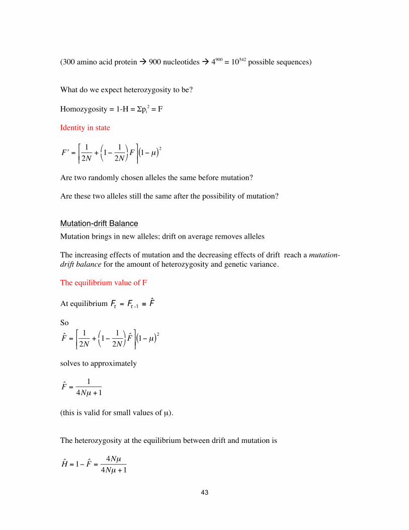
(300 amino acid protein à 900 nucleotides à 4900 = 10542 possible sequences) What do we expect heterozygosity to be? Homozygosity = 1-H = Σpi

2 = F Identity in state

€

" F =12N

+ 1− 12N

$ %

& '

F(

) * +

, - 1− µ( )2

Are two randomly chosen alleles the same before mutation? Are these two alleles still the same after the possibility of mutation?

Mutation-drift Balance Mutation brings in new alleles; drift on average removes alleles The increasing effects of mutation and the decreasing effects of drift reach a mutation-drift balance for the amount of heterozygosity and genetic variance. The equilibrium value of F At equilibrium Ft = Ft −1 ≡ ˆ F So

€

ˆ F = 12N

+ 1− 12N

# $

% &

ˆ F '

( ) *

+ , 1− µ( )2

solves to approximately

€

ˆ F = 14Nµ +1

(this is valid for small values of µ). The heterozygosity at the equilibrium between drift and mutation is

€

ˆ H = 1− ˆ F =4Nµ

4Nµ +1

44

Neutral Theory The idea that many mutations have little or no effect Due to Motoo Kimura. For neutral alleles, the substitution rate equals the mutation rate. Why? The substitution rate can be found by multiplying the number of new mutations per locus per population per generation times the probability that a single new mutation fixes. For a new mutation, the allele frequency is p = 1/2N. For a neutral allele, the probability of fixation is p. # of new mutations/locus/population/generation = 2Nµ. New mutation fixed per generation = 2N µ (1/2N) = µ.

Measuring mutation rates Possible ways:

• Directly observe changes from one genotype to another • Assume selective neutrality - measure substitution rates • Accumulate mutations over many generations to magnify the effects

Mutation accumulation experiments A way to measure mutational effects on fitness or some other quantitative character (both the rate of mutation and the effects of those mutations) Therefore it is important to eliminate selection (to keep and measure the deleterious mutations as well). One way is to use balancer chromosomes.

• Contain inversions, which suppress recombination • Have dominant alleles for some easily seen phenotype • Have recessive lethal allele (to kill homozygotes of the balancer)

45

These balancer chromosomes were developed to more easily maintain sick chromosomes in culture Cy (Curly) is a balancer for the 2nd chromosome in Drosophila melanogaster. Pm (Plum) is a dominant mutation in D. melanogaster, also on the 2nd chromosome. (Male Drosophila don't have recombination.)

...CyPm

CyPm

Pm+

multiple lines with exactly the same 2nd chromosome

Pm+

Pm+

Pm+

Pm+

Pm+

Pm+

MUTATION

for 70 generations

x

x

x CyPm

x CyPm

CyPm

x

x CyPm

x CyPm

46

Next, test the relative fitness of each mutation accumulation line:

The results:

Pm+

x CyPm

i

+Cy

i+

Cy

ix

+Cy

i +i

CyCy

+i

1 2 1: :

Die

Heterozygous Effects

Homozygous effects

47

Selection

Natural Selection The central idea of modern evolutionary biology, and Darwin's great contribution • There is almost always reproductive excess (more offspring are produced than can

survive and reproduce) • Organisms vary in their ability to survive and reproduce (i.e. in their fitness) • Genotypes with higher fitness leave more offspring, therefore these genotypes

increase in frequency

48

Fitness and Fitness Components

Zygote

Adult

Mating Pair

Gametes

Zygotes

Viability, survivorship

Sexual selection, mating success

FecundityFertility

Gametic selectionMeiotic Drive

49

Relative Fitness Fitness of a genotype, standardized to a reference genotype

Genotype Absolute Fitness Relative Fitness * AA 1.4 1.4/1.4 = 1 Aa 1.2 1.2/1.4 = 0.86 aa 0.8 0.8/1.4 = 0.57

* In this case, the fitnesses were standardized relative to the fitness of AA.

Measuring Selection Measuring the fitness of different genotypes can be very difficult • Each fitness component can be important, so all must be accounted for • Must eliminate random effects • Fitness can be genetically complex: dominance effects, interactions between loci, etc. • Statistical problems: 1% fitness difference can be very important, but very difficult to

reliably measure • Fitness effects can be very environmentally dependent, and therefore vary over time

and space

Simple Models of selection

Haploid selection 1 gene, 2 alleles Let A and B be the numbers of the 2 alleles with growth rates a and b, so

At = (1+a)t A0

Bt = (1+b)t B0

€

At

Bt

=1+ a( )t

1+ b( )tA0B0

= wt A0B0

where

€

w =1+ a( )1+ b( )

is the relative fitness of A.

50

Selection happens if a≠b.

If a > b , then the relative frequency of A will increase through time.

€

pt =At

At + Bt

=ptNt

ptNt + 1− pt( )Nt

€

pt =w pt−1

w pt−1 + 1− pt−1( )

Proof:

€

pt =At

At + Bt

=1+ a( )At−1

1+ a( )At−1 + 1+ b( )Bt−1

pt =w At−1

w At−1 + Bt−1

Divide the top and bottom by (At-1 + Bt-1):

€

pt =w pt−1

w pt−1 + (1− pt−1)

So population size cancels out in modeling the effects of selection (when the relative fitness is not a function of population size)

51

Change in allele frequency (haploids)

€

Δp = pt − pt−1 =w p

w p + q− p

=pq w −1( )w p + q

The Δp notation refers to " the change in p"

Diploid selection Let w11, w12, and w22 be the relative fitnesses of AA, Aa, and aa. Life cycle: Random mating à Hardy-Weinberg frequencies

p2 : 2pq : q2 à Differential survivorship

w11 p2 : w12 2pq : w22 q2 àStandardize to sum to 1

(w11 /

€

w ) p2 : (w12 /

€

w ) 2pq : (w22 /

€

w ) q2 where

€

w is the mean fitness of the genotypes:

€

w = w11 p2 + w12 2pq + w22 q2 The new allele frequencies are then found from these new genotype frequencies:

€

" p = " p 11 +" p 122

=p2w11 + pqw12

w

" q =q2w22 + pqw12

w

We can also write this as !p = p pw11 + qw12w

"

#$

%

&'

52

Additive effects Let's look at the case with no dominance (i.e. the heterozygote is exactly intermediate to the homozygotes in fitness) w11 = 1+2 s, w12 = 1+ s and w22 = 1 We refer to s as the selection coefficient.

!p =p2 1+ 2s( )+ pq 1+ s( )

p2 1+ 2s( )+ 2pq 1+ s( )+ q2 (1)

=p 1+ s+ sp( )1+ 2ps

Δ𝑝 = 𝑝! − 𝑝 =𝑝 1+ 𝑠 + 𝑠𝑝1+ 2𝑠𝑝 − 𝑝 =

𝑠𝑝𝑞1+ 2𝑝𝑠 ≈ 𝑠𝑝𝑞

Notice that Δp is a function of two aspects of biology: the strength of selection and the amount of genetic variation.

53

Response to Selection depends on the strength of selection and the genetic variance, so the rate of change of allele frequency increases with • greater selective differences • intermediate p

Equilibria Let the equilibrium allele frequency under selection be

€

ˆ p With no mutation or migration bringing in new alleles, p = 0 and p = 1 are always possible equilibria If w11 < w12 < w22 then pà0 If w11 > w12 > w22 then pà1 If w11 < w12 > w22 then there will be a stable intermediate allele frequency (overdominance) If w11 > w12 < w22 then pà1 or pà0, depending on the initial allele frequency (underdominance) Nature of equilibria: Unstable v. stable

Stable equilibrium: system moves to this point from nearby Unstable equilibrium: system doesn't change if exactly at this point, but moves away with a small perturbation. e.g. If w11 < w12 < w22 then p=0 is a stable equilibrium point, but p=1 is an unstable equilibrium point.

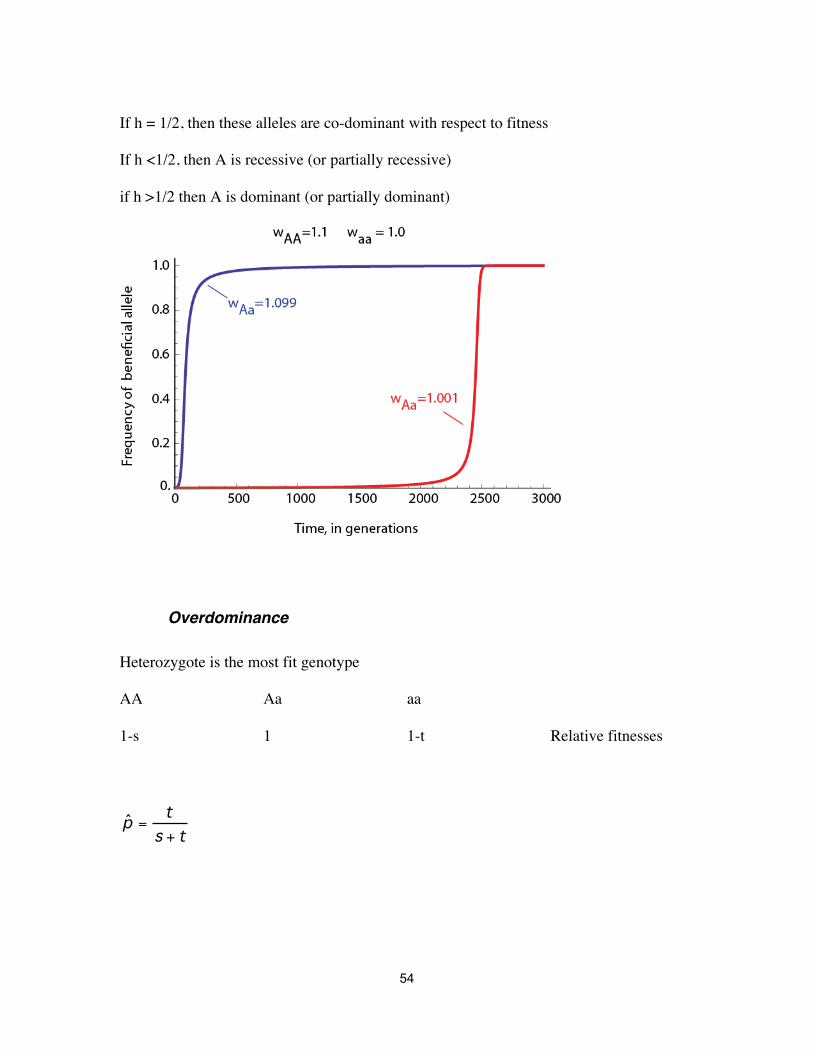
Dominance AA Aa aa 1+s 1+hs 1 Relative fitnesses

54

If h = 1/2, then these alleles are co-dominant with respect to fitness If h <1/2, then A is recessive (or partially recessive) if h >1/2 then A is dominant (or partially dominant)

Overdominance Heterozygote is the most fit genotype AA Aa aa 1-s 1 1-t Relative fitnesses

ˆ p = t

s + t

55

56

Overdominance can maintain genetic variation --- but relatively few examples are known. The classic example is β hemoglobin in humans: Two of the alleles of the β hemoglobin locus are A and S. Fitness * AA "normal" sensitive to malaria 0.89 AS heterozygote resistant to malaria,

slight sickling of red blood cells

1

SS sickle cell sickle cell anemia 0.2 • These are the fitnesses as measured in West Africa, in a malarial area

Multiple alleles and marginal fitness n alleles with frequencies p1, p2, p3, …pn Σpi = 1 Use the marginal fitnesses of the alleles

€

wi = wij p jj∑

57

which is the average fitness of an individual with allele i.

€

" p i =piwi

w

Fisher's Fundamental Theorem The rate of increase of mean fitness is equal to the additive genetic variance for fitness

€

Δw = VA The overall variance in fitness can be partitioned into genetic variance and environmental variance: VA and VE For fitness, VE >> VA The major implication of the fundamental theorem is that mean fitness increases by selection (so we can find equilibria by finding the maximum w .)

58

59

Assumptions of the fundamental theorem • No migration, mutation, or drift • Genes interact additively • Fitness effects are measured by the marginal effects of the alleles

wA = p wAA + q wAa

Sex specific selection Selection on alleles can vary between sexes Different ranks of fitness in males and females can act to maintain polymorphism.

Frequency - dependent selection Fitness of an allele depends upon the frequency of that allele e.g. coiling in snails or butterfly mimicry patterns Frequency dependence can be positive or negative

Positive Frequency dependence - Allele becomes more favored as it becomes more common

Negative Frequency dependence - Allele becomes less fit as it becomes more common

60

61

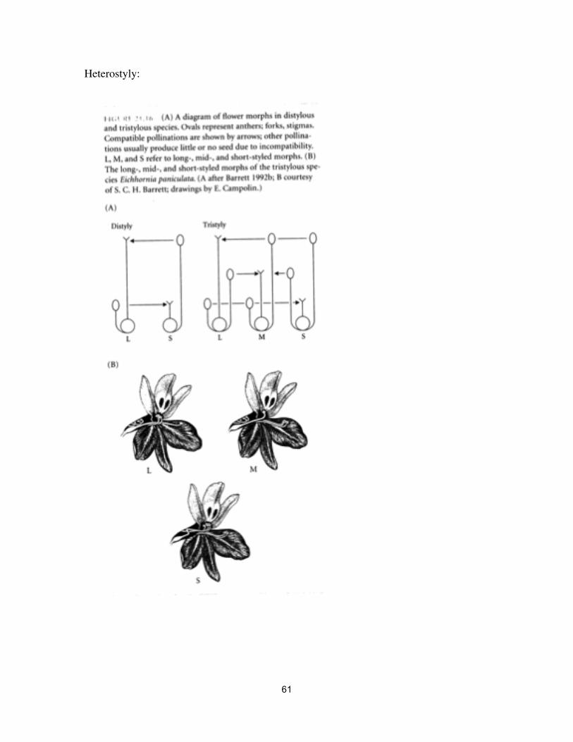
Heterostyly:

62

Density - dependent selection Relative fitnesses depend on population size e.g. Selection on reproductive strategy Feeding strategies

Sexual Selection Differential mating success 2 types

• Intrasexual competition (Usually male-male competition) e.g. stags fighting over mates

• Choice

(Usually female choice -- females choosing male mates) e.g. female peahens choosing peacocks with longer tails

63

Female choice in male traits can lead to exaggerated secondary sexual characteristics: e.g. tail length, waddle size, plumage coloration, louder calls, etc. Traits which increase mating success can evolve, even if they have some deleterious effects on survivorship e.g. Forked fungus beetles Males with longer horns on their back have higher mating success, but lower survivorship

Fecundity selection Relative fitnesses of alleles depend on producing differential numbers of offspring Models of fecundity selection are not generally solvable and are much more difficult

Meiotic drive Non-Mendelian production of gametes by heterozygotes

€

" p = p2 + 2kpq If k≠1/2, then meiotic drive is occurring. Meiotic drive has been observed many times: e.g. t alleles in mice Segregation distorter (SD) in flies

Aa

A a

adults

gametes

k 1-k

64

Gametic selection • differential success of gametes e.g. pollen survival

sperm competition (including sperm displacement, differential swimming rate, etc.)

Differential selection on different fitness components e.g. Meiotic drive can be opposed by natural selection Selection can be different in gametes and diploid phases Viability selection can be different from fertility selection

Mutation-selection Balance Most mutations are deleterious and decrease in frequency by selection

What is the equilibrium allele frequency? AA Aa aa 1 1-hs 1-s Relative fitnesses e.g. Huntington's Disease w11 = 1, w12 = 0.81 and w22 = 0, so s= 1 and h = 0.19. a = deleterious allele

Frequency of abad alleleMutation Selection

65

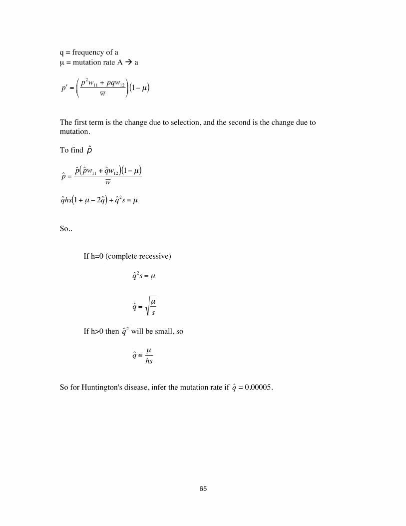
q = frequency of a µ = mutation rate A à a

€

" p =p2w11 + pqw12

w #

$ %

&

' ( 1− µ( )

The first term is the change due to selection, and the second is the change due to mutation. To find ̂ p

€

ˆ p =ˆ p ˆ p w11 + ˆ q w12( ) 1− µ( )

w

€

ˆ q hs 1+ µ − 2ˆ q ( ) + ˆ q 2s = µ So..

If h=0 (complete recessive)

€

ˆ q 2s = µ

ˆ q = µs

If h>0 then

€

ˆ q 2 will be small, so

€

ˆ q ≅ µhs

So for Huntington's disease, infer the mutation rate if

€

ˆ q = 0.00005.

66

€

ˆ q ≅µhs

0.00005 ≅ µ1( ) 0,19( )

µ ≅ 9.5x10−6

Mutation Load The reduction in the mean fitness of a population due to deleterious mutations w no mutations( ) ≡1w with mutations( ) =1− q2s for h = 0( )

q2 = µs

#

$%

&

'(

2

=µs

)

*

++

,

-

.

.

so

w h = 0( ) =1− µs

#

$%

&

'(s =1−µ

€

Load = w no mutations( ) − w mutations( )= µ

Note that this load is independent of s. (What's the load for mutations with h>0? 2μ ) In general the load is the number of mutations that come in per individual (2μ ) divided by the number of mutations killed by an average selection event. This number of mutations removed per selective death is 2 for homozygous effects and 1 for heterozygous effects.

Drift and Selection Genetic drift can obscure the deterministic process of selection. (In finite populations, the most fit allele does not always go to its deterministic equilibrium)

67

In small populations, drift can allow a deleterious allele to fix in a population. The reduction in fitness this causes is called drift load.

68

69

Fixation of beneficial alleles Even in large (or infinite) populations, a new mutation is present in only a few copies and is therefore likely to be lost by chance The probability of fixation of a new beneficial allele is only 2s, where s is the increase in fitness of the heterozygotes. In a non-ideal population, this probability becomes 2s Ne / N. Note that by “new beneficial allele” we mean an allele that is present as a signle copy, i.e. at frequency p = 1/(2N).

Fixation more generally Probability of fixation of a new mutation (present initially as a single copy):

u ≅1− exp −2sNe / N[ ]1− exp −4sNe[ ]

with fitnesses 1:1+s:1+2s. Even when the allele is deleterious (i.e. s<0) there is some probability of fixation by chance.

70

Selection at multiple loci If the fitness effects of two loci interact multiplicatively, then the 2-locus dynamics are completely described by the dynamics of each locus separately i.e. wAaBB = wAa wBB etc.

Epistasis If the genes interact in some other way, we say that there is epistasis, and the changes at one locus affect what happens at the other à This tends to cause linkage disequilibrium (with an excess of the most fit genotypes), which is in turn broken down by recombination So the fundamental theorem need not apply (because the genes are interacting in complex ways). Mean fitness need not be maximized. BUT -- it turns out that if selection is weak and recombination is strong, then the fundamental theorem is very close to the right answer.

Example: Moraba scurra, a grasshopper from Australia polymorphic for two inversions on two different chromosomes. Fitnesses

BB BB' B'B' AA 0.79 1.00 0.83 AA' 0.67 1.006 0.90 A'A' 0.66 0.66 1.07

71

Detecting selection on proteins There are many tests of selection at the protein level. One very commonly used approach is the McDonald-Kreitman test, which asks whether there are more coding changes between species than you would expect based on the variation within species. The McDonald-Kreitman test compares synonymous and non-synonymous differences within and among species, looking for an excess of coding changes between species. The null model of the McDonald-Kreitman test, with no selection causing divergence between the species: Within species

(Polymorphism) Among species (Divergence)

Synonymous

4 Ne μS

2 t (μS)

Non-synonymous

4 Ne μN f

2 t (μN) f

where

Ne is the effective population size μS is the mutation rate to synonymous codons μN is the mutation rate to non-synonymous codons

72

f is the fraction of mutations which are not deleterious (the method assumes that deleterious alleles are efficiently removed from the population and are not observed.)

t is the number of generations since the common ancestor of the two species (so that there have been 2t generation s of evolution separating them, because both species have been evolving separately for t generations.)

These calculations assume that the polymorphism of a particular type is predicted by 4 Ne μ, and that the substitution rate per generation of neutral mutations is the mutation rate per individual, as shown by Kimura. (Hence the divergence is proportional to the number of generations in which a substitution could have occurred(2t) times the substitution rate per generation (μ).) Note that the rows and columns of this table can be constructed by the product of a term for the column (4Ne or 4t) and a term for the row (μS or μN f). This means that to test this null model, we can use a contingency analysis; we can count the number of differences between individuals within or between species, and separate those into synonymous or non-synonymous differences. A contingency test allows a statistical test of whether this null model fits. For example, McDonald and Kreitman (1991) looked at the Alcohol dehydrogenase gene in Drosophila melanogaster. Looking at the DNA sequence in the coding region of this gene (and comparing it to the sequence form other Drosophila species), they found: Within species

(Polymorphism) Among species (Divergence)

Synonymous

42

17

Non-synonymous

2

7

This shows a statistical significant excess of non-synonymous changes between species (P = 0.006), and so evidence of adaptive evolution at this locus. Adam Eyre-Walker and his colleagues have taken this one step further. Comparing synonymous and non-synonymous changes across many genes in many species, they have estimated the fraction of amino acid changes between species that are due to positive selection. Their estimates range from about 0% in some plants to 10% in humans to up to 50% in rodents or flies.

73

Inbreeding Inbreeding is the mating of relatives - a form of non-random mating Inbreeding alone does not change allele frequencies, but inbreeding does change genotype frequencies. Inbreeding can affect allele frequencies, by changing how selection operates f: Inbreeding coefficient: the probability that 2 alleles in the same individual are identical by descent.

Calculation of F from pedigrees Inbreeding—and the probability of identity by descent of two alleles in an individual—comes from cases when the two alleles in an individual may have the same ancestor. For example, in the following pedigree, the individual at the bottom descends has two great-grandparents which are the same individual.

74

The probability that 2 alleles in individual I are identical by descent is (1/2)5(1+fA). There can be multiple paths through a pedigree: f is the sum of the probabilities from all of these paths

1/2 (1+FA)

1/2

1/2

1/2

1/2

A

B C

D E

I

75

fI = (1/2)5(1+fA) +(1/2)5(1+fB)

A B

C D

E G

I

A B

C D

E G

I

A B

C D

E G

I

76

Genotype frequency changes with inbreeding Main result: Excess Homozygotes Remember the example of self-fertilization:

We can measure inbreeding by the reduction of heterozygosity

f = (H0 −H )H0

,

where H0 is the heterozygosity of a randomly mating population with the same allele frequencies. For the bi-allelic case, H0 = 2 pq, so H = 2pq(1-f).

Genotype frequencies with inbreeding

AA Aa aa

Genotype

Genotype frequencies

Self-fertilization

Genotype frequencies next generation

AA Aa aa

x y z

AA x AA Aa x Aa aa x aa

AA Aa aa

x+y/4 y/2 z+y/4

1/41/2

1/4

77

p2 + fpq 2pq(1-f) q2 + fpq pF +(1-f)p2 2pq(1-f) qf+(1-f)q2

i.e. 1/2 the "missing" heterozygotes become AA and 1/2 become aa, which leave the allele frequency unchanged: p = p2 + pqf +pq (1-f) = p2 + pq = p(p + q) = p

Relationship between inbreeding and drift As a population is divided into separate groups, each of size N, mating becomes non-random (i.e. mating only occurs within groups) Therefore the probability that an individual has 2 alleles which are identical by descent goes up as f' = 1/2N +(1-1/2N)f

Inbreeding and fitness Inbred individuals usually have lower fitness than outbred individuals. This reduction in fitness with inbreeding is called inbreeding depression.

€

δ =woutbred − winbred

woutbred

78

Why is there inbreeding depression? 2 possible reasons: (1) deleterious recessive alleles (2) overdominance In both cases, heterozygotes are more fit than the average of the homozygotes, and inbreeding increases homozygosity

Inbreeding depression by deleterious recessives Genotype AA Aa aa Frequency in outbreds

p2 2pq q2

Frequency in inbreds

p2 + fpq 2pq(1-f) q2+ fpq

Fitness 1 1 1-s

€

w outbred = p2 + 2pq + q2 1− s( )= 1− sq2

79

winbred = p2 + fpq+ 2pq 1− f( )+ q2 + fpq( ) 1− s( )

=1− s q2 + fpq( ) < woutbred

The effects of inbreeding on selection Inbreeding alone does not affect allele frequency; but it can influence the outcome of selection Why? Because an excess number of homozygotes are produced, and selection on homozygotes can be different from that on heterozygotes

e.g. Selfing A fraction S of a population selfs each generation, and 1-S outcross (mate at random): Let x, y, and z be the frequencies of AA, Aa, and aa:

€

" x =1− S( ) p2 + S x +

y4

$ % &

' ( )

* + ,

- . / w11

w

" y =1− S( )2pq + S

y2$ % & ' ( )

* + ,

- . /

w12

w

" z =1− S( )q2 + S z +

y4

$ % &

' ( )

* + ,

- . / w22

w

where

€

w = 1− S( )w outbred + S w inbred

w inbred = w11 x +y4

# $

% &

+ w12y2# $ % &

+ w22 z +y4

# $

% &

80

With sufficient selfing in a population, the internal equilibrium with overdominance moves towards more of the allele with the fitter homozygote, and the internal equilibrium can disappear. This is because the homozygote fitness matters more and more with selfing, because more alleles are expressed in homozygotes than expected with random mating.

81

Hybrid Vigor = Heterosis Increased fitness of outcrossed individuals e.g. hybrid corn increases yield 15-30%

Mixed Mating Model Some individuals self S Some outcross 1-S With complete selfing: ft+1 = 1/2 (1+ft) With partial selfing: ft+1 = 1/2 (1+ft) S At equilibrium:

f̂ = S 12!

"#$

%& 1+ f̂( )

f̂ = S2− S

which is used to estimate selfing rates.

Evolution of Inbreeding and inbreeding avoidance Many adaptations have evolved to avoid inbreeding (and inbreeding depression) e.g. tristyly, self-incompatibility alleles, sequential hermaphrodism, sex-biased dispersal There are also many adaptations for selfing; e.g. cleistogamous (closed) flowers), small flowers, anthers close to stigma, etc.

Evolution of selfing There are obvious costs to selfing (inbreeding depression) But also advantages: • Reproductive assurance (don’t need others to reproduce) • Cost of outcrossing (producing offspring is expensive - why share with other genes?) Individuals which self and act as males to other individuals get 3/2 as many alleles into the next generation, all else being equal

82

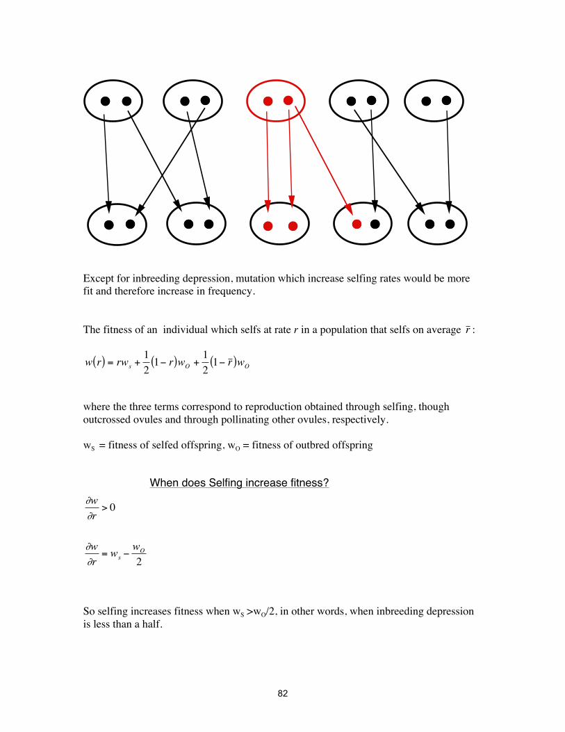
Except for inbreeding depression, mutation which increase selfing rates would be more fit and therefore increase in frequency. The fitness of an individual which selfs at rate r in a population that selfs on average

€

r :

€

w r( ) = rws +121− r( )wO +

121− r ( )wO

where the three terms correspond to reproduction obtained through selfing, though outcrossed ovules and through pollinating other ovules, respectively. wS = fitness of selfed offspring, wO = fitness of outbred offspring

When does Selfing increase fitness?

€

∂w∂r

> 0

∂w∂r

= ws −wO

2

So selfing increases fitness when wS >wO/2, in other words, when inbreeding depression is less than a half.

83

Inbreeding changes the frequency of deleterious mutations For deleterious recessives, selfing exposes the homozygous alleles to selection much more often

€

ˆ q selfing ≈µs

< ˆ q outcrossin g ≈µhs

So inbreeding depression will lessen with selection à "purging"

84

85

Therefore repeated inbreeding can create the conditions for selfing to evolve -- But this says that you have to have selfing to evolve selfing!

Other factors can allow for, or select for selfing • Isolation à A colonizing individual may have no one else to mate with (most weeds

are selfers) • Other inbreeding à small population size can also result in a reduction in inbreeding

depression

Assortative mating Positive assortative mating à "like mates with like"à positive correlation of mates e.g. flowering time, human height, IQ

Negative assortative mating à negative correlation of parents e.g. heterostyly, self-incompatibility alleles

86

Positive assortative mating tends to increase homozygosity Negative assortative mating tends to increase heterozygosity, and usually acts as negative frequency dependence

Sex Ratio Evolution A population of nearly all females with just enough males to allow fertilization has the highest possible intrinsic growth rate.

So -- Why so many males? Because • All offspring have one male parent and one female parent • If males are rare, than males will have a high fitness relative to females (males would

contribute more of the genes of the next generation • Same in reverse, if females are rare Fisher showed that this causes an equal sex ratio

versus

87

Subsequently it has been shown that this result holds regardless of the mechanism of sex determination (e.g. chromosomal sex determination, genic sex determination, environmental sex determination) More precisely, mothers will equalize investment in reproductive male and female offspring (which resolves the apparent contradictions in the Hymenoptera) Exceptions: If mating occurs among close relatives before mixing with the general population, this selects for female-biased sex ratios • This is called local mate competition e.g. fig wasps, Nasonia parasitic wasps

88

Population Structure

Migration and Population Structure deme - semi-isolated sub-population

Wahlund Effect The number of homozygotes in 2 separate populations is equal to or greater than the number in a randomly mating mixture of these 2 populations

F in subdivided populations AA Aa aa Population 1 p1

2 2 p1 q1 q12

Population 2 p22 2 p2 q2 q2

2

Pooled Populations (p12+ p2

2)/2 p1 q1 + p2 q2 (q12 + q2

2)/2 Pooled (in terms of F)

p2 1− f( )+ pf 2pq 1− f( ) q 2 1− f( )+ qf

This F we call FST.

€

p12 + p2

2

2= p 2 1− FST( ) + p FST

E p2[ ] = p 2 + FST p − p 2( )E p2[ ]− p 2 = FST p q

Var p[ ] = FST p q

0.2 0.4 0.6 0.8 1

0.1

0.2

0.3

0.4

0.5

p2p1

2pq

89

€

FST =Var p( )p 1− p ( )

90

2-locus Wahlund Effect Differences in allele frequencies at 2 loci in multiple populations generates linkage disequilibrium

Wright's F-statistics Population structure leads to increased homozygosity Inbreeding within subpopulations also increases homozygosity Wright's F-statistics can describe the effects of both Definitions: HI : heterozygosity of an individual in a subpopulation (averaged over subpopulations) HS : Expected heterozygosity of an individual in a randomly mating subpopulation with the same allele frequencies (averaged over subpopulations) = 2 pi qi HT: Expected heterozygosity of an individual in a randomly mating total population (given the average allele frequency of the total population)

€

= 2p q

91

FIS

Inbreeding coefficient within subpopulations

€

FIS =H S − HI

H S

FIS à inbreeding coefficient of individuals within subpopulations

FST

Measure of the non-random mating among subpopulations

€

FST =HT − H S

HT

FST à inbreeding among subpopulations (S) within the total population (T) GST is another measure of the genetic differences among subpopulations, but which allows for multiple alleles

FIT

Overall inbreeding coefficient

€

FIT =HT − HI

HT

€

1− FIT( ) = 1− FST( ) 1− FIS( ) For outcrossing organisms, FIS is usually small (<0.01) FST is variable among species (0 à 0.4)

Nei's D (Note - this D does not mean linkage disequilibrium) Another measure of the genetic differentiation of 2 populations "Genetic distance"

92

Migration and Selection Consider the simple situation where there is one-way migration from a mainland to an island. The mainland is fixed for an allele A, which is less fit on the island than another allele a.

What is the allele frequency on the island?

€

Δqmig = −mq

Δqsel =pqw12 + q2w22

w − q

There will be an equilibrium when

€

Δqmig + Δqsel = 0 a will be able to invade the island if s > m, where s is the selective benefit on the island of Aa over AA

93

Migration and Drift

Migration -drift balance; the island model

Each deme has N individuals and a proportion m of the individuals are migrants. Assumptions: • No selection • No mutation • All populations are the same size: N • All populations contribute m of their individuals to the migrant pool • All populations have m of their individuals arriving as migrants per generation • Migration is random with respect to distance

€

" F ST =12N

+ 1− m( )2 1− 12N

$ %

& '

FST

94

€

FST =12N

+ 1− m( )2 1− 12N

# $

% & FST

# $ '

% & (

FST 1− 1− m( )2 1− 12N

# $

% &

# $ '

% & ( =

12N

FST =1

2N 1− 1− m( )2( ) 1− 12N

# $

% &

≅1

4Nm +1

FST is often related to the number of migrants per generation by the formula

€

FST =1

4Nm +1

Migration is a potent way of reducing the genetic variance among populations. e.g. if Nm = 1 (one migrant per generation) then FST =0.2, which is not as much inbreeding as one generation of sib-mating. So in principle, we can estimate something about the rate of dispersal:

€

Nm =1 FST −1

4

95

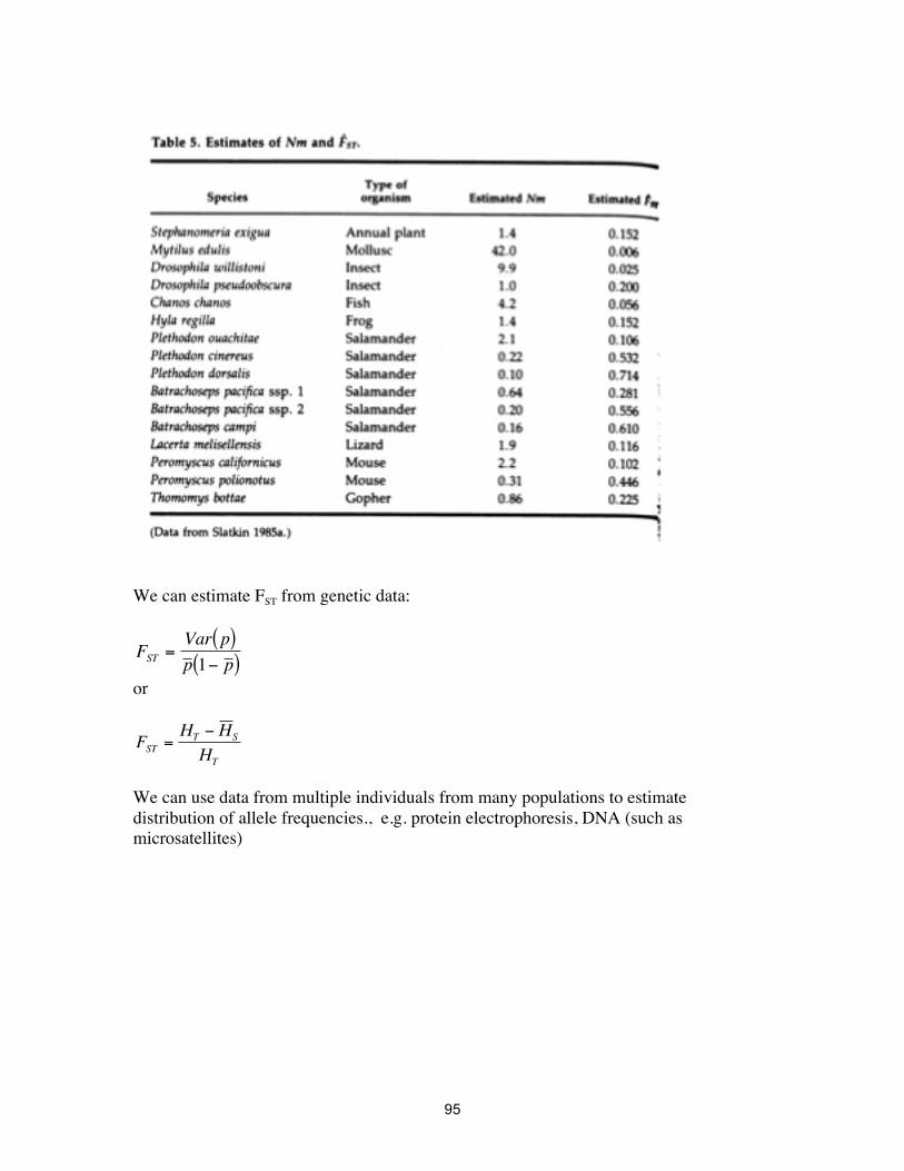
We can estimate FST from genetic data:

€

FST =Var p( )p 1− p ( )

or

€

FST =HT − H S

HT

We can use data from multiple individuals from many populations to estimate distribution of allele frequencies., e.g. protein electrophoresis, DNA (such as microsatellites)

96

BUT..... there are two problems: • The real world is not like the island model • Even the island model is not always like the island model: statistical problems

97

The real world is not like the Island model-- take the assumptions one by one:

• All populations are created equal, with N individuals and equal contributions to the migrant pool -

⇒ Population sizes are extremely variable, both in space and time

⇒ Populations are variable in their contributions to the migrant pool (e.g. sources and sinks)

⇒ populations vary through time in migration rates

• There is NO spatial structure: in effect all populations are equally close to all other populations (no isolation by distance)

⇒ Dispersal is almost always distance related; there is isolation by distance

⇒ Dispersal is also often affected by other factors: rivers, roads, mountains, etc.

• Everything is at equilibrium, nothing is changing. ⇒ Populations often go extinct, and new ones form by

colonization ⇒ History matters -- often the circumstances which determine

the current population structure are the conditions of the past, which may have changed

⇒ There may be migration in from outside the study system, changing allele frequencies over time

• No selection ⇒ There’s ALWAYS selection

• no mutation ⇒ Mutation can be at very fast rates, for example in

microsatellites

98

The island model is not always like the island model

• For mitochondrial markers (or others inherited uniparentally) FST = 1/(2Nm+1)

• The statistical properties of FST are not well worked out, but they’re ugly - see the figures

• Dispersal rates for genetic purposes are often quite different than what is

needed for ecological studies ⇒ Genetic dispersal only counts if the migrants reproduce effectively ⇒ Genetic dispersal only counts if the reproduction of migrant

individuals is equal to resident individuals (i.e., migrants have to move before their reproductive life starts)

⇒ Selection can over-amplify migrant genetic contributions • Problems of scale : Genetic analysis only tells you about migration at the

geographical scale at which the samples are drawn from.

99

Island Model with Migration, Mutation, Selection, and Drift

€

ψ p( ) = C p4 Nµ +4Nmp −1q4Nν +4Nmq −1W 2N

This is Wright's distribution.

100

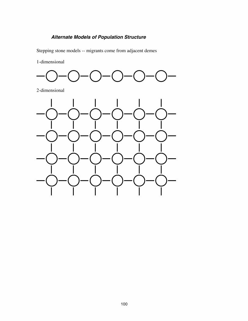
Alternate Models of Population Structure Stepping stone models -- migrants come from adjacent demes 1-dimensional

2-dimensional

101

Local adaptation Environments are heterogeneous at many spatial scales One patch of habitat will be different from any other patch Populations may adapt to local conditions Cline - a steady change in allele frequency across a geographic region

Step cline - a cline with a more sudden change in allele frequency

p

N S

p

N S

102

Trifolium

Cyanide production reduces herbivory, but when cells freeze and burst, this releases cyanide to within the clover itself.

103

Agrostis tenuis - bent grass

These plants were taken from seeds on plants only 7 m apart, in mine tailings and just outside Strong selection Agrostis selfs, so reduced recombination with other types

104

Culex pipiens Organophosphate pesticides applied near south coast of France beginning in 1972 In 1973, a resistant allele of esterase appeared which could metabolize the pesticide In the 1980's, the broad scale application of the pesticide stopped In 1987, an allele of acetocholineesterase appeared which was even more resistant.

105

106

Evolution on complex landscapes Adaptive landscape - graph of the function which relates mean fitness of a population to its genotype or phenotype frequencies Q: If mean fitness always increases as a result of selection, AND there is a valley between two peaks, how can a population evolve from one local fitness maximum to another?

Possible answers: (1) Mean fitness function changes as a result of environmental changes (2) Changes in other loci may change fitness interactions (3) Wright's shifting balance process

-2 -1 0 1 2

0.20.40.60.81

1.21.4

MeanFitness

Mean Phenotypic Value

107

Wright's Shifting Balance theory suggests that drift in local populations can allow a shift from one adaptive peak to another. Three phases:

Phase I: Drift

0.20.40.60.81

1.21.4

MeanFitness

Mean Phenotypic Value

x'x

108

Phase II: Selection within demes

Phase III: Interdemic selection

Problems with the SBT • Sufficient drift probably occurs very rarely • Response to interdemic selection is weak

0.20.40.60.81

1.21.4

MeanFitness

Mean Phenotypic Value

x'x

109

Kin Selection Any event which increases the frequency of an allele due to the properties of that allele is selection. If the effect of this selection is to increase the fitness of relatives, this is called kin selection. e.g. worker ants, parental care r = coefficient or relationship of 2 individuals (= 2F/(1+F) where F is the inbreeding coefficient of offspring of those two individuals) A trait will evolve by kin selection if c < r b c: cost to its own fitness b: benefit to relative's fitness

Group selection Kin selection is a special case of group selection Groups of organisms may have differential survivorship (i.e. different extinction rates) and/or differential fertility (i.e. different emigration rates) If groups are genetically differentiated, this allows for gene frequency change as a result of the properties of groups. Broad scale group selection is probably a small factor in allele frequency change Because FST's are relatively small, change in allele frequency due to group selection is likely much smaller than the change due to individual selection

110

Introduction to Quantitative Genetics

What’s a “quantitative character”? A quantitative character is a trait which exhibits continuous variation.

Why study continuous variation, when we know the genetic basis of traits is discrete?

Even with a relatively small number of genes involved, the variation for a character will often appear continuous, due to measurement error and, more importantly, environmental effects.

Who cares? • Most characters are continuously distributed. • We do not fully understand the genetic basis of most traits, therefore we must describe them statistically. • Even with better understanding of the genetic basis of a trait, a statistical description of that trait can be extremely useful. • Quantitative genetic understanding has allowed substantial gains in agricultural output. • QG concepts has allowed new understanding of evolutionary processes.

111

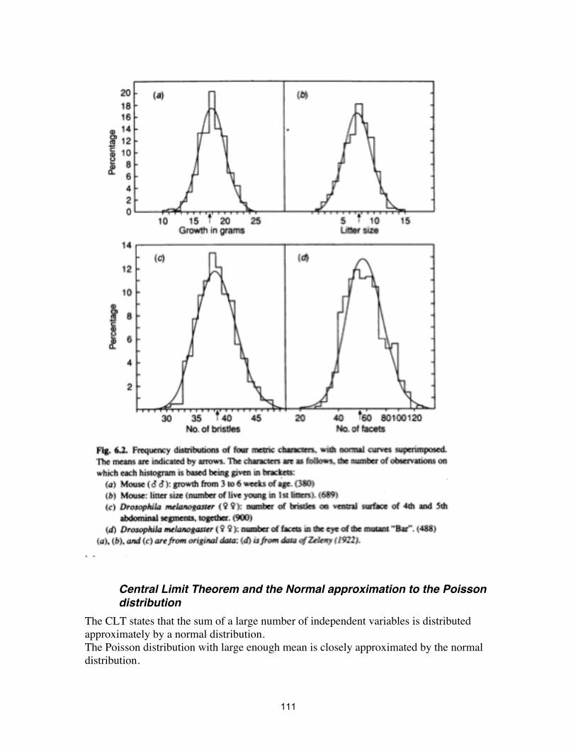
Central Limit Theorem and the Normal approximation to the Poisson distribution

The CLT states that the sum of a large number of independent variables is distributed approximately by a normal distribution. The Poisson distribution with large enough mean is closely approximated by the normal distribution.

112

Resemblance between relatives is in part a function of sharing alleles

113

Response to Selection and the correlation of relatives The response to selection is predicted by the heritability and the selection differential: R = h2 S. Truncation Selection Truncation selection is simply taking all of the individuals above a certain threshold value.

114

Definitions: regression and correlations The correlation of X and Y is defined as the covariance of X and Y divided by the standard deviations of X and Y. (This is the square root of the coefficient of determination.)

ρXY =

Cov X, Y[ ]SD X[ ]SD Y[ ] .

The regression coefficient of Y on X is the covariance of X and Y divided by the variance of X. This is the slope of the regression of Y on X.

115

bXY =

Cov X ,Y[ ]Var X[ ]

Mid-parent offspring regression Define the mean of the two parents as the mid-parent.

€

bOP =Cov[O,P ]

Var[P ]=

VA

VP

Heritability The heritability is one of the most important quantitative genetic properties. It predicts the response to selection, and expresses the reliability of the phenotype in determining the breeding value. Definitions Heritability is represented by h2. The narrow-sense heritability is defined as

€

h2 =VA

VP

Variance is a property of the population; therefore the heritability is a function of the population, as well as of the character. Variances must be non-negative. VA ≤ VP. Therefore, the heritability must be between 0 and 1.

116

Predicting response to selection

Components of the phenotypic variance

Average Effect

The average effect is the mean deviation from the population mean of individuals which received that allele from on parent, when the other allele is chosen at random from the population.

Breeding Value

The value of an individual, as measured by the average value of its offspring, is called its breeding value. This is twice the deviation of the offspring from the population mean (since the individual only contributes half of the alleles to its offspring). This is also the sum of the average effects of the individual. With random mating, the mean breeding value is zero.

Dominance

The genetic effects (G) can be further partitioned. Ignoring interactions among loci, G=A+D. In this equation, the A refers to the additive effects, which is the sum of the breeding values, and the D refers to dominance deviations. These dominance deviations refer to the deviation of diploid genotypic values from the sum of the average effects of those genotypes, due to the interaction between alleles at the same locus.

Interaction

If different loci interact to form the phenotype, then there is epistasis, and this interaction affects the composition of phenotypes in the population.

117

Components of variance

€

VP = VG +VE

= VA +VD +VI +VE

VP= Phenotypic Variance VG= Genetic Variance VE= Environmental Variance VA= Additive genetic Variance VD= Dominance Variance VI= Epistatic Variance

Heritability: the proportion of variance which is determined by genetics. Broad-sense heritability: VG/VP. Narrow-sense heritability: VA/VP. *** This is the important one, generally.

Analysis of variance

The partitioning of variance follows an ANOVA kind of logic. In fact ANOVA’s were invented for exactly this reason by R. A. Fisher.

Additive, dominance, epistatic variance

Having the additive variance be greater than zero does not imply that alleles interact additively. Even with complete dominance, or with complete epistasis, there will usually be additive variance.

118

Correlations and interactions between G and E

G and E can be correlated (i.e. “good” offspring being provisioned more); more importantly, there can be interaction terms.

Estimating heritability by the resemblance among relatives There are two ways of estimating heritability. 1. By examining the covariance among relatives. 2. By measuring the response to selection. There are various problems with using correlations of relatives to estimating heritability: 1. There can be common environmental effects. 2. There can be maternal effects. 3. All of the covariances include epistatic variance terms; many also include dominance variance. 4. Measurement error. 5. Assortative mating can skew results. 6. Differences in the variance of the different sexes must be accounted for.

• Consider the problems of each type of relatives Intuition: Relatives resemble one another. Why? Because they share genes and because they share environments.

119

Genetic Covariance among relatives

Parent-offspring

The regression of the mean value of offspring on the value in a parent:

€

bOP =Cov[O,P]Var[P]

=12VA

VP

Notice that this is equal to half the heritability! Define the mean of the two parents as the mid-parent. In this case, the covariance of offspring with the mid-parent is also 1/2 VA. But the variance among mid-parents is equal to VP/2, so the regression of offspring on mid-parent is equal to the heritability:

€

bOP =Cov[O,P ]

Var[P ]=

VA

VP

Half-sibs

The covariance among half-sibs is

€

Cov Half − sibs[ ] =14VA .

Full-sibs (Dominance rears its ugly head)

The covariance among full sibs turns out to be:

Cov Full sibs[ ] = 12VA +14VD

This is because full sibs share not only alleles, but also can have the same genotype at a greater than random rate. Think of it as this: full sibs have a 1/2 probability of sharing alleles, so the contribution of the additive variance (i.e. that due to single allelic effects) to the covariance is half the additive variance. Furthermore, they have a 1/4 chance of sharing the same genotype, therefore they “share” 1/4 of the dominance variance.

Identical Twins

Identical (or monozygotic) twins share all of their genes and genotype, so the genetic covariance among twins is equal to VG.

120

Environmental covariance among relatives Here’s a problem: family members are likely to experience similar environments as well. Therefore there is likely to be some covariance among relatives which is due to environmental effects, not genetical effects. Hence we can naïvely overestimate heritability and VA.

Common environmental effects

Common environmental effects are those environmental effects which different groups (such as families) experience in common. Represented by VEc. These can be huge. Examples: varying food quality, common density, cultural effects (i.e. wealth in humans) These can completely skew genetic variance component estimations. The covariance among any class of relatives is equal to the genetic covariance plus the common environment variance. Thus if we measure VA in half sibs by multiplying the covariance times 4, we would also be multiplying the error introduced by VEc by a factor of 4 as well. This is a huge problem for studies on humans, where these sorts of environmental covariances cannot be controlled for. Controlling for VEc in other experiments is a major source of expense, since it requires offspring to be raised separately. Competition is a particularly bad source of common environmental effects; it can even cause negative covariances.

Maternal effects

Maternal effects are the covariances that result from the maternal environment. Mothers contribute not only genes to their offspring, but also cytoplasm, nutrients, and sometimes parental care. These factors can co-vary with the mother’s condition, and therefore a source of environmental variation can result in pernicious covariance. This can be controlled for partially by using half-sib designs, with the sire as the common parent, by cross-fostering, and by comparing maternal covariance to paternal covariance.

Assortative mating Assortative mating, the mating of like with like, results in inflated estimates of heritability. For example, the covariance of parents and offspring is inflated by a factor of (1+r) where, confusingly, r is the correlation of phenotypic values of mates. Intuition: If mates are correlated, then the offspring of those individuals will be not only correlated with parents because of the alleles they inherit from that parent, but also because the alleles they inherit from the other parent have a higher than average probability of being the same as well.

121

Response to Selection The response to selection (i.e. the difference in the mean of one generation from the mean of the previous generation) is directly proportional to the heritability. Selection on Quantitative Characters

122

123

Response to selection The response to selection is the change in the population mean after selection. -> R Selection Differential The selection differential is the difference in the mean of the selected parents from the mean of the population as a whole. -> S

Intensity of Selection This is just a standardized version of the selection differential; i.e., the selection differential divided by the standard phenotypic deviation of the trait. -> i

Measuring the response to selection

Variability among generations Selected lines vary substantially in their response to selection even from one generation to the next. WHY?

Error

Measurement error can result in substantially variable results. Selection on behavioral traits, or other traits with low repeatability, result in noise among generations in means.

Drift

Selection experiments are normally done with relatively small population sizes, because of the resource costs of measuring individuals. Therefore, there is a lot of latitude for genetic drift.

124

Environmental variance

Environmental conditions vary through time: this is why it is essential to have controls.

Asymmetry of response

Selection experiments are often done in both directions; i.e. up and down for the same trait. It is often the case that there is an asymmetry of the response to selection. In morphology, the lines for increased size often show more response than those for decreased size. There are several reasons for this asymmetry.

125

Drift

Drift can cause the cumulative response in one direction to be greater than the other. This often cannot explain a repeated bias in response in one direction across replicate lines, but must be rejected as a null hypothesis.

Natural selection

If there is stronger natural selection for the trait in one direction than the other, then natural selection will aid artificial selection n direction and hinder it in another.

Scale effects: the variance may change as a function of the mean

The genetic variance may scale as a function of the mean of the trait, and therefore the variance may be reduced in one direction, and therefore the response to selection.

Inbreeding depression

As lines become more selected in selection experiments, then the lines also typically become more inbred, for a variety of reasons. If there is directional dominance then this will result in a bias in response to selection.

“Genetical asymmetry”: Gene frequencies divergent from p=0.5

If allele frequencies for genes which affect the trait are on average different from p = q = 0.5, then there will be an asymmetry of the amount to which selection can respond and how fast.

Special case: Genes of large effects If much of the variance for a trait is due to a few important loci, then if the frequencies of even just those loci deviate from p = 0.5, then the asymmetry of response will also be seen

Non-linear interactions of genes and environments

Genotype-by-environment interactions can result in different effects of genes at different allele frequencies.

126

Long-term selection

Selection limits

Theoretical limits: the sum of the best alleles in the starting population

This depends on the number of loci contributing to the genetic variance.

Changes in phenotypic variance Phenotypic variance often increases as a result of selection. This may be due to inbreeding effects on the environmental variance.

Mutation generates new variance At equilibrium, the long-term response to selection allowed by mutation is R= S 2Ne VM/VP. This is because the variance coming into the population per generation is 2Ne VM, where VM is the mutational variance per haplotype per generation. A typical value for VM is approximately 10-3 VE.

What limits selection response?

Physical or logical constraints The value in question cannot be greater or less than a certain physical limit, such as a proportion cannot be greater than 1 or less than 0.

Natural, or correlated, selection Natural selection can limit the response to artificial selection.

Changes in the partitioning of variance (i.e. variance due to recessive alleles)

Dominance When the unfavored recessives reach low frequencies, much of the variance is non-additive, and therefore not available for selection response.

Overdominance In the (unlikely) event that the favored phenotype is produced by heterozygotes, then this also results in a lack of additive variance.

Exhaustion of genetic variance -- the effect of population size Obviously, if selection “uses up” all of the genetic variance, then the response will slow. Larger populations allow more genetic variance.

127

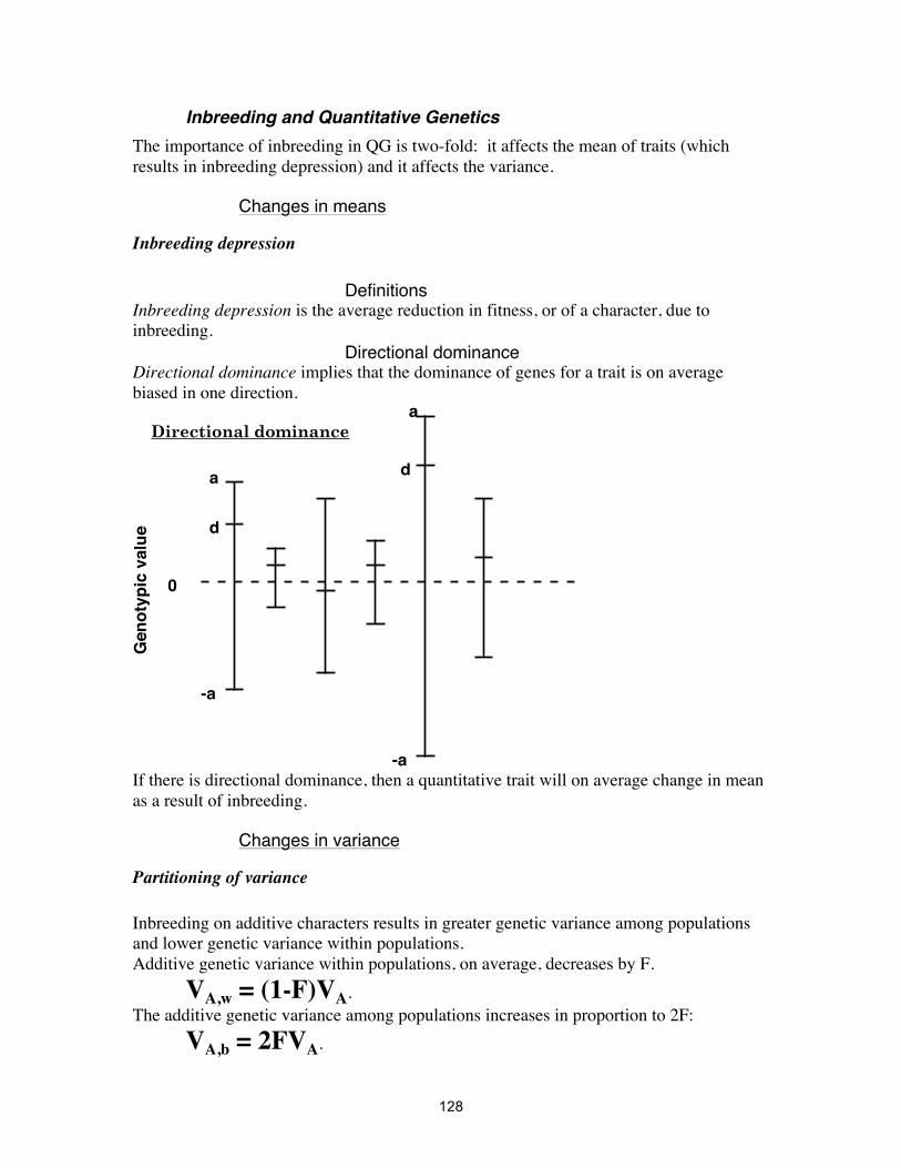
128

Inbreeding and Quantitative Genetics The importance of inbreeding in QG is two-fold: it affects the mean of traits (which results in inbreeding depression) and it affects the variance.

Changes in means

Inbreeding depression

Definitions Inbreeding depression is the average reduction in fitness, or of a character, due to inbreeding.

Directional dominance Directional dominance implies that the dominance of genes for a trait is on average biased in one direction.

If there is directional dominance, then a quantitative trait will on average change in mean as a result of inbreeding.

Changes in variance

Partitioning of variance

Inbreeding on additive characters results in greater genetic variance among populations and lower genetic variance within populations. Additive genetic variance within populations, on average, decreases by F.

VA,w = (1-F)VA. The additive genetic variance among populations increases in proportion to 2F:

VA,b = 2FVA.

0

a

-a

d

a

-a

d

Directional dominance

Gen

otyp

ic v

alue

129

The total additive genetic variance is therefore VA,w + VA,b = (1+F)VA.

The heritability within lines is expected to decrease as a result of this reduction in VA.

Changes in VE

Sensitivity to environmental perturbations increases with inbreeding; in other words, there is inbreeding depression for homeostasis.

130

Correlated Characters Characters are often correlated, that is, the phenotypic value of one character in an individual is correlated with the phenotypic value of another character on that individual. (The circumference of your head is about 1/3 of your height.) These correlations can also be due to environmental effects or genetic effects. The genetic causes of correlation are pleiotropy (that genes affect more than one character) and linkage disequilibrium. This need not be constant across genes: some genes can cause positive pleiotropy and others negative pleiotropy; the balance determines the genetic correlation of the two characters. The sign of the genetic correlation need not be the same as the phenotypic correlation.

131

Correlated response to selection Selection on one trait will often result in response for another trait. This is due to genetic correlations. Selection on one trait can cause an apparent selection differential at another trait, because of both the genetic and environmental correlations. This is a particularly huge problem when studying natural selection in natural conditions.

Indirect selection Selecting for one character to get a response in another.

132

133

Evolutionary Quantitative Genetics

Fisher’s Fundamental Theorem of Natural Selection So the response to selection for fitness is given by

RW =VA W[ ]

Correlated Response to Natural Selection By a similar derivation, the correlated response to selection on fitness for a character is given by

CRY = Cov A Y ,W[ ]

Evolutionary QG in a nutshell

Trait vectors and the G matrix

z is the vector of phenotypic values (i.e. {z1, z2, z3, ...} where each of these z’s is the value of some character. G is the genetic variance-covariance matrix:

VA X[ ] Cov A X,Y[ ]Cov A X ,Y[ ] VA Y[ ]!

" #

$

% &

The P matrix, similarly, is the phenotypic variance-covariance matrix.

134

The Response to Selection

The strength of selection on can be described for multivariate selection as well:

s = z * − z where the * indicates the value after selection. Then there is a formula which describes the change in the mean from one generation to the next, analogous to R=h2 S:

Δz = GP−1s The value β = P-1 s is called the selection gradient. It is equivalent to the vector of partial regression coefficients of relative fitness on character states.

Measuring the Strength of Selection Two basic problems to all methods of measuring selection: (1) There are always unmeasured characters, which may explain the true relationship of fitness and phenotype and have correlated effects on the characters studied. (2) Fitness is hugely difficult to measure.

135

Stabilizing Selection

Definition

Selection for some intermediate value of the trait.

Effects

Stabilizing selection acts to reduce the phenotypic variance of the trait. It does this by increasing the canalization of the trait, as well as by reducing the genetic variance for the trait. Canalization is the reduced sensitivity of an organism to noise from the environment. Genetic variance can be reduced in two ways:

• By creating negative correlations of allelic effects: linkage disequilibrium. • By changing gene frequencies to be closer to fixation.

136

Disruptive selection

Selection against intermediates

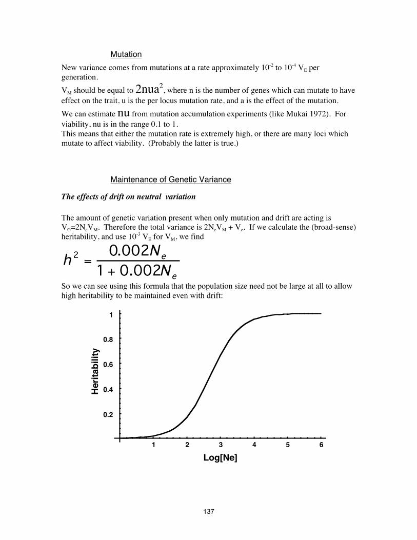
137

Mutation New variance comes from mutations at a rate approximately 10-2 to 10-4 VE per generation. VM should be equal to 2nua2, where n is the number of genes which can mutate to have effect on the trait, u is the per locus mutation rate, and a is the effect of the mutation. We can estimate nu from mutation accumulation experiments (like Mukai 1972). For viability, nu is in the range 0.1 to 1. This means that either the mutation rate is extremely high, or there are many loci which mutate to affect viability. (Probably the latter is true.)

Maintenance of Genetic Variance

The effects of drift on neutral variation

The amount of genetic variation present when only mutation and drift are acting is VG=2NeVM. Therefore the total variance is 2NeVM + Ve. If we calculate the (broad-sense) heritability, and use 10-3 VE for VM, we find

h 2 =

0.002Ne1 + 0.002Ne

So we can see using this formula that the population size need not be large at all to allow high heritability to be maintained even with drift:

1 2 3 4 5 6

0.2

0.4

0.6

0.8

1

Log[Ne]

Heritability