Biologically Inspired AdaptiveControl of Quadcopter Flight

by

Brent Komer

A thesispresented to the University of Waterloo

in fulfillment of thethesis requirement for the degree of

Master of Mathematicsin

Computer Science

Waterloo, Ontario, Canada, 2015

c© Brent Komer 2015

I hereby declare that I am the sole author of this thesis. This is a true copy of the thesis,including any required final revisions, as accepted by my examiners.

I understand that my thesis may be made electronically available to the public.

ii

Abstract

This thesis explores the application of a biologically inspired adaptive controller toquadcopter flight control. This begins with an introduction to modelling the dynamics of aquadcopter, followed by an overview of control theory and neural simulation in Nengo. TheVirtual Robotics Experimentation Platform (V-REP) is used to simulate the quadcopterin a physical environment. Iterative design improvements leading to the final controller arediscussed. The controller model is run on a series of benchmark tasks and its performance iscompared to conventional controllers. The results show that the neural adaptive controllerperforms on par with conventional controllers on simple tasks but exceeds far beyond thesecontrollers on tasks involving unexpected external forces in the environment.

iii

Acknowledgements

First off, I would like to thank my supervisor, Chris Eliasmith, for his guidance andsupport throughout my research. My thanks extends to the rest of the members of theCentre for Theoretical Neuroscience, for all of their help and for making this lab a greatenvironment to work in. I would also like to thank Jeff Orchard and Edith Law for takingthe time to read through this thesis. Finally, I’d like to thank my friends and family. Inparticular Sally Siu for all of her support and encouragement.

iv

Dedication

To my family, for their unending support and love.

v

Table of Contents

List of Tables ix

List of Figures x

Glossary xii

1 Introduction 1

1.1 Motivation . . . . . . . . . . . . . . . . . . . . . . . . . . . . . . . . . . . . 1

1.2 Quadcopters . . . . . . . . . . . . . . . . . . . . . . . . . . . . . . . . . . . 2

2 Background Information 4

2.1 Flight Control . . . . . . . . . . . . . . . . . . . . . . . . . . . . . . . . . . 4

2.2 Dynamics . . . . . . . . . . . . . . . . . . . . . . . . . . . . . . . . . . . . 5

2.3 Simulation . . . . . . . . . . . . . . . . . . . . . . . . . . . . . . . . . . . . 8

3 Control 10

3.1 PID Control . . . . . . . . . . . . . . . . . . . . . . . . . . . . . . . . . . . 10

3.2 Adaptive Control . . . . . . . . . . . . . . . . . . . . . . . . . . . . . . . . 11

3.3 Neural Simulation . . . . . . . . . . . . . . . . . . . . . . . . . . . . . . . . 12

3.4 Adaptive Control in Nengo . . . . . . . . . . . . . . . . . . . . . . . . . . . 14

vi

4 Design 15

4.1 Derivation of Non-Neural Adaptive Controller . . . . . . . . . . . . . . . . 15

4.2 Controller Implementation . . . . . . . . . . . . . . . . . . . . . . . . . . . 18

4.3 Iterations . . . . . . . . . . . . . . . . . . . . . . . . . . . . . . . . . . . . 19

4.3.1 Gain Tuning . . . . . . . . . . . . . . . . . . . . . . . . . . . . . . . 24

4.3.2 Using Hyperopt . . . . . . . . . . . . . . . . . . . . . . . . . . . . . 25

4.3.3 Improving Adaptation to Horizontal Forces . . . . . . . . . . . . . . 26

4.3.4 Shortcomings of the Error Signal . . . . . . . . . . . . . . . . . . . 27

4.3.5 Additional State Information . . . . . . . . . . . . . . . . . . . . . 30

4.4 Software Simulation . . . . . . . . . . . . . . . . . . . . . . . . . . . . . . . 31

5 Simulations and Results 33

5.1 Experiments . . . . . . . . . . . . . . . . . . . . . . . . . . . . . . . . . . . 33

5.1.1 Metrics . . . . . . . . . . . . . . . . . . . . . . . . . . . . . . . . . 33

5.1.2 Benchmarks for Simple Environments . . . . . . . . . . . . . . . . . 35

5.1.3 Benchmarks for Complex Environments . . . . . . . . . . . . . . . . 39

5.1.4 Improvement over Time . . . . . . . . . . . . . . . . . . . . . . . . 41

5.2 Results . . . . . . . . . . . . . . . . . . . . . . . . . . . . . . . . . . . . . . 41

6 Discussion and Future Work 44

6.1 Contributions . . . . . . . . . . . . . . . . . . . . . . . . . . . . . . . . . . 44

6.2 Discussion . . . . . . . . . . . . . . . . . . . . . . . . . . . . . . . . . . . . 44

6.3 Future Work . . . . . . . . . . . . . . . . . . . . . . . . . . . . . . . . . . . 46

6.3.1 Adaptive Prediction System . . . . . . . . . . . . . . . . . . . . . . 46

6.3.2 Integrated Navigation and Planning System . . . . . . . . . . . . . 47

6.3.3 Detailed Modelling . . . . . . . . . . . . . . . . . . . . . . . . . . . 47

6.3.4 Realistic Sensors . . . . . . . . . . . . . . . . . . . . . . . . . . . . 47

6.3.5 Running on Physical Hardware . . . . . . . . . . . . . . . . . . . . 48

6.4 Conclusion . . . . . . . . . . . . . . . . . . . . . . . . . . . . . . . . . . . . 48

vii

APPENDICES 49

A Link to the Source Code 50

References 51

viii

List of Tables

2.1 Robotic Simulator Candidates . . . . . . . . . . . . . . . . . . . . . . . . . 8

4.1 Gain Values Obtained Through Hyperopt . . . . . . . . . . . . . . . . . . . 26

5.1 Controller Models . . . . . . . . . . . . . . . . . . . . . . . . . . . . . . . . 34

5.2 Benchmark Tasks . . . . . . . . . . . . . . . . . . . . . . . . . . . . . . . . 36

5.3 Forcing Functions . . . . . . . . . . . . . . . . . . . . . . . . . . . . . . . . 39

5.4 Mean Controller Performance . . . . . . . . . . . . . . . . . . . . . . . . . 43

ix

List of Figures

2.1 Four Primary Quadcopter Movements. Taken from [17] . . . . . . . . . . . 5

2.2 The Inertial and Body Frames of a Quadcopter. Taken from [23] . . . . . 6

2.3 Simulation Environment in V-REP . . . . . . . . . . . . . . . . . . . . . . 9

4.1 Basic Quadcopter Controller Network . . . . . . . . . . . . . . . . . . . . . 20

4.2 Simplified Quadcopter Controller Network . . . . . . . . . . . . . . . . . . 20

4.3 Quadcopter Controller Network with Adaptation . . . . . . . . . . . . . . 21

4.4 Performance of Original Adaptive Controller . . . . . . . . . . . . . . . . . 22

4.5 Zero Control Signal Region . . . . . . . . . . . . . . . . . . . . . . . . . . . 23

4.6 Quadcopter Controller Network with Adaptive Transformation . . . . . . . 24

4.7 Performance of Basic Adaptive Controller . . . . . . . . . . . . . . . . . . 27

4.8 Quadcopter Controller Network with Angle Correction . . . . . . . . . . . 28

4.9 Performance of Angle Correction Controller . . . . . . . . . . . . . . . . . 28

4.10 Quadcopter Controller Network with Target Modulated Control . . . . . . 29

4.11 Performance of Filtered Angle Correction Controller . . . . . . . . . . . . . 30

4.12 Quadcopter Controller Network with Allocentric Target Modulated Control 31

5.1 Controllers used in Benchmarking . . . . . . . . . . . . . . . . . . . . . . . 36

5.2 Performance on Horizontal Movement Tasks . . . . . . . . . . . . . . . . . 37

5.3 Performance on Vertical Movement Tasks . . . . . . . . . . . . . . . . . . . 37

5.4 Performance on Rotational Movement Tasks . . . . . . . . . . . . . . . . . 38

x

5.5 Performance on Horizontal Movement Through Wind Tasks . . . . . . . . 38

5.6 Performance on Benchmarks under different External Force Conditions . . 40

5.7 Path of Quadcopter between Two Points with External Forces . . . . . . . 41

5.8 Controller Performance Ranking . . . . . . . . . . . . . . . . . . . . . . . . 42

6.1 Horizontal Motion with Noise . . . . . . . . . . . . . . . . . . . . . . . . . 45

6.2 Circular Path with External Forces . . . . . . . . . . . . . . . . . . . . . . 46

xi

Glossary

Connection A link between the output of one Ensemble or Node to the input of anotherEnsemble or Node.

Decoders Weightings applied to neural activities to produce a vector.

Encoders Functions applied to a vector to produce neural activities.

Ensemble A group of neurons representing a single vector.

Nengo A Python software package that implements algorithms from the Neural Engineer-ing Framework.

Network A group of Ensembles, Nodes, Connections, and other Networks within a Nengomodel.

Neural Engineering Framework A set of methods for performing computations withsimulated ensembles of neurons.

Node A component of a Nengo network that executes Python code rather than represent-ing a value.

Synapse A filter applied to a connection between two representational components inNengo.

Tuning Curve Response characteristics of a neuron.

xii

Chapter 1

Introduction

1.1 Motivation

Humans have an exceptional ability to be able to adapt to their surroundings. In particularthe human motor control system is able to compensate for changes in forces, torques, andinertial effects on the body. For example, when picking up an object such as a hammer,the weight of the hammer will apply external forces to the hand. This will change thedynamic properties of the hand and arm movements, yet the human motor control systemis able to easily compensate for these changes and accurately control movement with theobject. Even if an object has never been encountered before, the human brain is able tocalculate the correct changes in timing and muscle tensions in order to skilfully manipulatethe object. The predictive capabilities of the brain, along with the plasticity of neuralconnections in the motor area help guide these sophisticated behaviours.

This ability for quick and easy adaptation to new dynamic properties of a system wouldbe extremely useful in robotics. Applying similar methods of control that have been devel-oped over millions of years of evolution in the brain to a robotic control system could resultin major improvements. This is especially useful now that the demands of many roboticsystems are now more general purpose than they were in the past. Robots started outmainly performing simple and repetitive tasks in stable environments, such as automationin manufacturing [15]. Now they are being used increasingly in more complex situationsrequiring a diverse amount of control, such as search and rescue missions, performing med-ical procedures, and assisting the elderly [15, 20, 25, 22]. When the precise environmentthat the robot will operate in is not fully known, it is useful for any control system thatthe robot uses to be adaptable to those environments.

1

Another advantage the brain has when it comes to control, is that it uses very littlepower, about 20 Watts on average [18]. Hardware inspired by the brain is being designed totake advantage of this low power paradigm. This style of hardware, known as neuromorphichardware, is typically massively parallel and consumes much less power than traditionalhardware. The algorithms explored in this thesis focus on being adaptive and biologicallyinspired in order to take advantage of such hardware.

1.2 Quadcopters

Quadcopters are very versatile aerial vehicles, typically consisting of a central body withfour upright rotors equally spaced around the body. This configuration allows them to belightweight and simplifies construction. They also have the ability to take off and landvertically without external assistance, meaning they can be used in a lot more situationsthan aircraft that require a runway or other particular conditions to take off. They canalso change directions fairly easily mid flight, and have the ability to hover at a particularlocation. Due to their low cost, light weight, and ease of use, they are an excellent aircraftto use for research purposes.

Despite all of these positive qualities, one of the main weaknesses of quadcopters istheir short battery life. Small and simple quadcopters used by hobbyists typically lastonly 5 to 10 minutes before they run out of power [2]. The more expensive industrialgrade quadcopters typically last up to 30 minutes before they need to be recharged, butthis duration is still not long enough for some applications. For example, if a quadcopteris being used in a search and rescue mission it may need to remain flying for a long timewithout recharging, especially if it is operating in a remote area. Battery weight is oneof the main issues hindering the maximum flight time of quadcopters. If a larger batteryis used in attempts to increase the maximum flight time, the quadcopter will be heavierand therefore require more power to fly, which in turn will drain the battery faster. Twopossible solutions to this problem are lighter batteries and more energy-efficient operation.The latter can be achieved by the use of neuromorphic hardware to run the flight controlsystem. While the majority of the power consumed by a quadcopter goes towards therotors, some is still used by the on-board control system. As the sophistication of thecontrol system increases, the computational demands will follow, leading to less overallflight time. Computational efficiency improvements in traditional digital computation isbeginning to stagnate and is expected to soon approach a limit where minimal improvementis expected. On the contrary, computational power efficiency for biological systems is 8-9orders of magnitude better than the power efficiency for digital computation [19]. Reducing

2

the power required for the control system can allow more of the power from the batteriesto be used for the rotors.

In addition to the low power consumption of neuromorphic hardware, they also have theadvantage of using various types of neural algorithms that can be extremely useful for con-trol. In particular, the learning capabilities of brain-like algorithms can be used to developcontrollers that are able to adapt to unknown environments with non-linear dynamics.This thesis explores an adaptive control algorithm for quadcopter flight constructed usingsimulated biologically plausible neurons.

Chapter 2 gives an overview of how quadcopters are able to fly, followed by a sectiondetailing the mathematics underlying the dynamics of a quadcopter system. Followingthe mathematical characterization is a description of how the quadcopter is modelled in asimulation environment. Chapter 3 gives an overview of the control theory used in devel-oping the control system, including standard PID control, adaptive control, and adaptivecontrol in a simulated biological neural system. Chapter 4 covers the initial design of thecontroller model, as well as many of the iterations of improvements leading to the finaldesign. Chapter 5 describes the set of experiments performed and metrics used to quantifyperformance of the various controllers. The final section discusses the results and outlinesareas of future work.

3

Chapter 2

Background Information

2.1 Flight Control

The system state of a quadcopter is six dimensional: three for position (x, y, and z)and three for orientation (roll, pitch, and yaw). There are four control inputs, which aretypically taken to be the rotational velocity of each of the four rotors. For a physicalquadcopter, these inputs are the voltages applied to each of these rotors. A transformationin these voltages can be obtained using the physical rotor parameters to estimate the rotorvelocity. For simplicity of the simulation, the velocity is used directly as the control inputin this thesis.

The rotors will always generate a thrust that is perpendicular to the body of the aircraft.In addition to this thrust, torque is generated by each rotor based on their spin directionas well as their distance from the center of the body. For the quadcopter to be able tocontrol its orientation, half of the rotors spin clockwise and the other half spin counter-clockwise. The pairs diagonally opposite each other across the body spin in the samedirection, allowing the torques to balance one another out and the quadcopter to maintaina steady orientation. By varying the relative speeds of each rotor, the quadcopter is ableto create a net torque in a specific direction, causing a rotation about any axis.

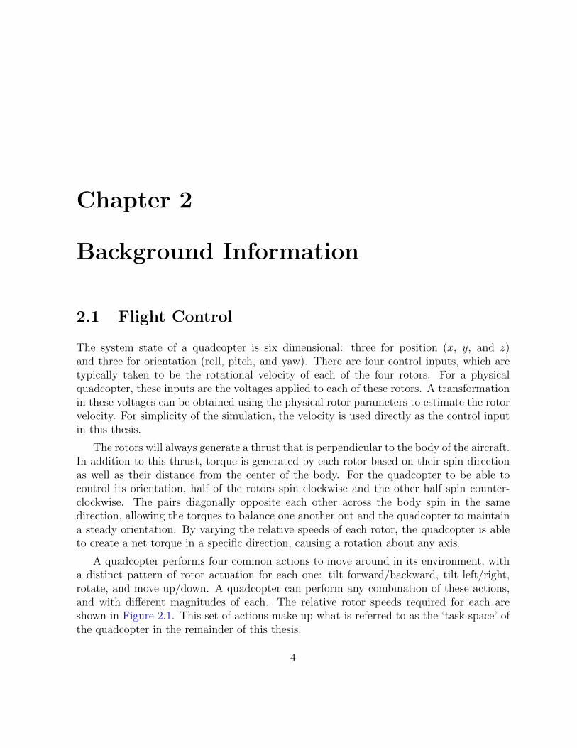
A quadcopter performs four common actions to move around in its environment, witha distinct pattern of rotor actuation for each one: tilt forward/backward, tilt left/right,rotate, and move up/down. A quadcopter can perform any combination of these actions,and with different magnitudes of each. The relative rotor speeds required for each areshown in Figure 2.1. This set of actions make up what is referred to as the ‘task space’ ofthe quadcopter in the remainder of this thesis.

4

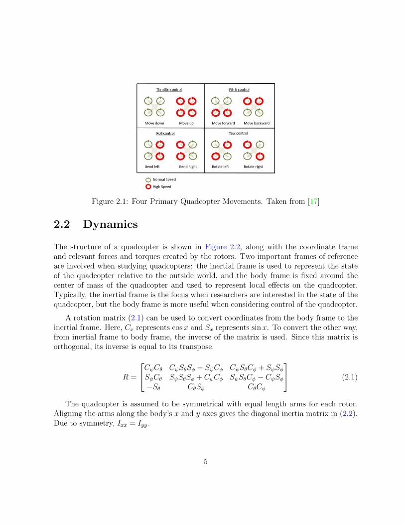
Figure 2.1: Four Primary Quadcopter Movements. Taken from [17]

2.2 Dynamics

The structure of a quadcopter is shown in Figure 2.2, along with the coordinate frameand relevant forces and torques created by the rotors. Two important frames of referenceare involved when studying quadcopters: the inertial frame is used to represent the stateof the quadcopter relative to the outside world, and the body frame is fixed around thecenter of mass of the quadcopter and used to represent local effects on the quadcopter.Typically, the inertial frame is the focus when researchers are interested in the state of thequadcopter, but the body frame is more useful when considering control of the quadcopter.

A rotation matrix (2.1) can be used to convert coordinates from the body frame to theinertial frame. Here, Cx represents cosx and Sx represents sinx. To convert the other way,from inertial frame to body frame, the inverse of the matrix is used. Since this matrix isorthogonal, its inverse is equal to its transpose.

R =

CψCθ CψSθSφ − SψCφ CψSθCφ + SψSφSψCθ SψSθSφ + CψCφ SψSθCφ − CψSφ−Sθ CθSφ CθCφ

(2.1)

The quadcopter is assumed to be symmetrical with equal length arms for each rotor.Aligning the arms along the body’s x and y axes gives the diagonal inertia matrix in (2.2).Due to symmetry, Ixx = Iyy.

5

Figure 2.2: The Inertial and Body Frames of a Quadcopter. Taken from [23]

Ixx 0 00 Iyy 00 0 Izz

(2.2)

The angular velocity of each rotor generates a thrust force perpendicular to the bodyframe, as well as a torque about the rotor axis. This relationship is shown in (2.3) and(2.4), where ω is the angular velocity of the ith rotor, k is the lift constant, b is the dragconstant, and IM is the rotor’s moment of inertia.

fi = kw2i (2.3)

τMi= bω2

i + IM ωi (2.4)

Typically the effect of the angular acceleration is considered small and is omitted inmost analyses, so it will not be present in the remainder of the dynamics derivations. Thisis because during steady state flight the rotors will be maintaining a constant (or almostconstant) velocity and will have approximately zero acceleration [16].

Note that the forces and torques generated are always proportional to the square ofthe rotor’s angular velocity, thus working with this term instead of the angular velocityitself is simpler. The set of values making up the square of the rotor angular velocities isreferred to as the ‘rotor space’ in the remainder of this thesis.

Combining the forces of all four rotors leads to (2.5), where T is the thrust in thedirection of the z-axis of the body. Combining the torques of all four rotors leads to (2.6),

6

where the vector τB represents the torques across each of the principal body axes (τφ forroll, τθ for pitch, and τψ for yaw). The distance between the rotor and the center of massof the quadcopter is denoted by l.

T =4∑i=1

fi = k

4∑i=1

w2i , TB =

00T

(2.5)

τB =

τφτθτψ

=

lk(−w22 + w2

4)lk(−w2

1 + w23)∑4

i=1 τMi

(2.6)

The governing equation for translational motion is (2.7); where ξ is the linear positionvector, TB is the thrust from (2.5), R is the rotation matrix from (2.1), A(ξ) is a matrixcontaining the drag force, and G is the gravitational force.

mξ = TBR− A(ξ)ξ −G (2.7)

Expanding (2.7) and setting the equation in terms of translational acceleration leadsto (2.8). xy

z

=T

m

CψSθCφ + SψSφSψSθCφ − SψSφ

CθCφ

− 1

m

Ax|x| 0 00 Ay|y| 00 0 Az|z|

xyz

−0

0g

(2.8)

The governing equation for rotational motion is (2.10); where η is the Euler anglevector, I is the inertia matrix from (2.2), τB is the applied torque from (2.6), and C(η)ηis the centripetal force.

Iη = C(η)η + τB (2.9)

Expanding (2.9) and setting the equation in terms of angular acceleration leads to(2.10). φθ

ψ

=

(Iyy − Izz)θψ/Ixx(Izz − Ixx)φψ/Iyy(Ixx − Iyy)φθ/Izz

+

τφ/Ixxτθ/Iyyτψ/Izz

(2.10)

Equations (2.8) and (2.10) are used throughout the remainder of this thesis to modelthe dynamics of the quadcopter during flight.

7

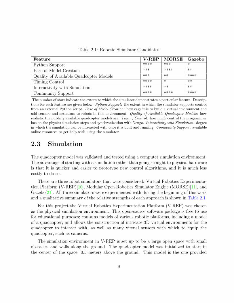
Table 2.1: Robotic Simulator Candidates

Feature V-REP MORSE GazeboPython Support **** *** *Ease of Model Creation *** **** **Quality of Available Quadcopter Models *** ** ****Timing Control **** * **Interactivity with Simulation **** ** **Community Support **** **** ****

The number of stars indicate the extent to which the simulator demonstrates a particular feature. Descrip-tions for each feature are given below. Python Support : the extent in which the simulator supports controlfrom an external Python script. Ease of Model Creation: how easy it is to build a virtual environment andadd sensors and actuators to robots in this environment. Quality of Available Quadcopter Models: howrealistic the publicly available quadcopter models are. Timing Control : how much control the programmerhas on the physics simulation steps and synchronization with Nengo. Interactivity with Simulation: degreein which the simulation can be interacted with once it is built and running. Community Support : availableonline resources to get help with using the simulator.

2.3 Simulation

The quadcopter model was validated and tested using a computer simulation environment.The advantage of starting with a simulation rather than going straight to physical hardwareis that it is quicker and easier to prototype new control algorithms, and it is much lesscostly to do so.

There are three robot simulators that were considered: Virtual Robotics Experimenta-tion Platform (V-REP)[10], Modular Open Robotics Simulator Engine (MORSE)[11], andGazebo[21]. All three simulators were experimented with during the beginning of this workand a qualitative summary of the relative strengths of each approach is shown in Table 2.1.

For this project the Virtual Robotics Experimentation Platform (V-REP) was chosenas the physical simulation environment. This open-source software package is free to usefor educational purposes; contains models of various robotic platforms, including a modelof a quadcopter; and allows the construction of intricate 3D virtual environments for thequadcopter to interact with, as well as many virtual sensors with which to equip thequadcopter, such as cameras.

The simulation environment in V-REP is set up to be a large open space with smallobstacles and walls along the ground. The quadcopter model was initialized to start inthe center of the space, 0.5 meters above the ground. This model is the one provided

8

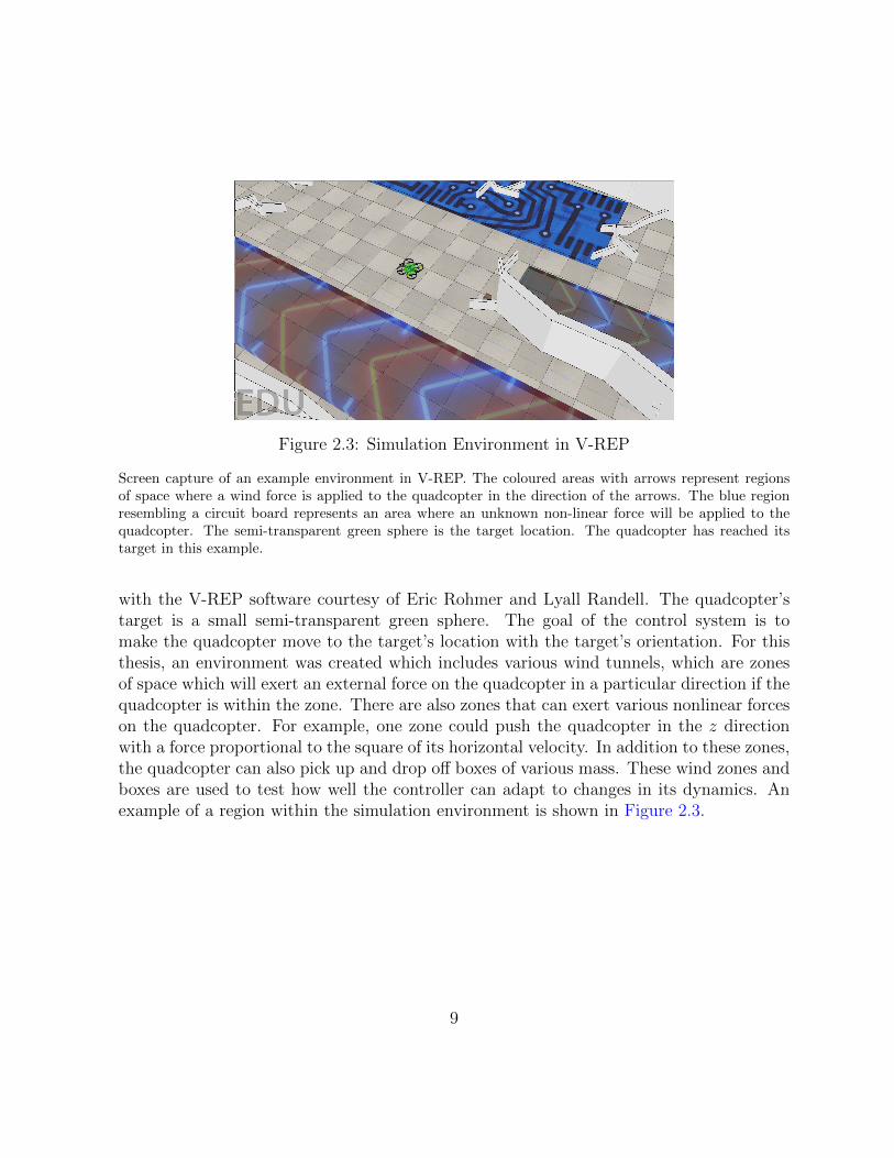
Figure 2.3: Simulation Environment in V-REP

Screen capture of an example environment in V-REP. The coloured areas with arrows represent regionsof space where a wind force is applied to the quadcopter in the direction of the arrows. The blue regionresembling a circuit board represents an area where an unknown non-linear force will be applied to thequadcopter. The semi-transparent green sphere is the target location. The quadcopter has reached itstarget in this example.

with the V-REP software courtesy of Eric Rohmer and Lyall Randell. The quadcopter’starget is a small semi-transparent green sphere. The goal of the control system is tomake the quadcopter move to the target’s location with the target’s orientation. For thisthesis, an environment was created which includes various wind tunnels, which are zonesof space which will exert an external force on the quadcopter in a particular direction if thequadcopter is within the zone. There are also zones that can exert various nonlinear forceson the quadcopter. For example, one zone could push the quadcopter in the z directionwith a force proportional to the square of its horizontal velocity. In addition to these zones,the quadcopter can also pick up and drop off boxes of various mass. These wind zones andboxes are used to test how well the controller can adapt to changes in its dynamics. Anexample of a region within the simulation environment is shown in Figure 2.3.

9

Chapter 3

Control

3.1 PID Control

The canonical method for building a control system is to use a PID controller. This is aclosed loop controller that works by applying gains to an error signal and feeding the resultas input to the plant (system being controlled). PID stands for Proportional, Integral, andDerivative, referring to the three types of gains used. One gain is applied directly to theerror (proportional); a second gain is applied to the derivative of the error, and the thirdgain is applied to the integral of the error. Each of these gains serves a unique purpose, andthe careful tuning of all three is required to get the desired performance of the controller.The proportional gain is the main driver of the system and responds directly to the error tobring the system towards its target point. The larger the gain, the faster this response willbe. However, using only this gain will not account for any inertia in the system and willoften cause the system being controlled to overshoot its target, especially when the gainis large. In some cases, the overshoot can be so large that the system becomes unstableand oscillates out of control. Thus, the derivative gain is usually used in addition, becauseit is sensitive to the rate of change of the error, and attempts to bring this rate towardszero. The faster the system is moving towards its target state, the more this gain acts toslow it down, by effectively providing a form of damping and so reducing the amount ofovershoot. Depending on how this parameter is tuned, and the properties of the systemat hand, it can remove overshooting entirely. Due to unmodelled disturbances or changingexternal inputs, there may be a steady-state error in the system, wherein the controllerhas reached a stable state, yet there is still an error being measured. The integral term isdesigned to account for this steady-state error by keeping a running sum of the error over

10

time. Eventually, this integral error should be large enough that it will drive the systemto close the steady-state error gap.

3.2 Adaptive Control

Sometimes the kinematics and dynamics of the system being controlled are unknown, orchange over time in an unknown fashion. A controller that works well for the systeminitially may not be well suited when the system undergoes changes. In this situation, itis useful to have a controller that can adapt to these changes.

The foundation of adaptive control is based on parameter estimation. First, a math-ematical model of the system to be controlled is generated based on physical laws. Thismodel is typically of the form shown in (3.1), where q is the vector of state variables, M(q)is a mass/inertia matrix, C(q, q) is the coriolis-drag term, g(q) is the gravitational force,and τ is a vector representing the input force/torque to the system.

M(q)q + C(q, q)q + g(q) = τ (3.1)

The goal of the controller is to bring the system to a particular target state. Typicallythe state as well as its derivative is desired to be controlled. Thus, the second derivativeof the state will be zero when the system has arrived at the target state. Setting q to bezero gives the relationship of the inputs to the rest of the state shown in (3.2).

τ = C(q, q)q + g(q) (3.2)

An estimate of q and q can typically be measured, leaving the only potentially unknownquantities in the right-hand side of the equation to be the physical parameters of the system.If these physical parameters are constant and linear with respect to the system state, theequation can be reorganized as in (3.3). Here θ is a vector of constant system parametersand Y (q, q) is a known matrix dependent on the system state. τ is the input required tokeep the system in a steady state.

τ = C(q, q)q + g(q) = Y (q, q)θ (3.3)

Often the system parameters are not fully known and an estimate needs to be usedinstead. Many control applications also require the system to be able to transition to

11

different states, rather than remain at a particular state. The adaptive control law in (3.4)uses an estimate of the parameter vector, θ, along with a standard control law to computethe desired input to the system. Here e is the state error and K is a gain matrix. Moredetail on this style of adaptive control law can be found in [28, 29, 9].

τ = Y (q, q)θ +Ke (3.4)

The parameter estimates can be initialized to any stable value and are updated ac-cording to the relationship in (3.5). L is a learning rate parameter that determines howquickly the parameter estimates change over time in proportion to the measured error.The parameter estimates will eventually converge on values that allow the system to becontrolled with minimal error. Given sufficient exploration of the state space, the param-eter estimates are guaranteed to converge to the real values if the real values are requiredfor optimal control [28].

˙θ = LY (q, q)TKe (3.5)

Creating a mathematical model of a system with enough detail to account for everythingis difficult. Assumptions and approximations must be made if the model is to be tractable.Moreover, external forces from the environment may influence the model, and their formmay be unknown as the environment can be largely unknown. One way to overcomethis problem is to use a set of basis functions as the model, and the weights applied toeach element of the basis as the constant parameters. If the basis is designed such thatit can represent any computable function to a reasonable degree of accuracy, it will beeffective in the adaptive control problem. Gaussian basis functions are commonly used inadaptive control [26], but neural networks may be used as well [4]. This thesis explores theapplication of this form of control law using basis functions that are biologically plausiblespiking neurons.

3.3 Neural Simulation

The Neural Engineering Framework (NEF)[14] provides a means of representing arbitraryvectors using the properties of neurons as a basis. This is done through a nonlinear encodingmechanism carried out by the tuning curves of the neurons, and a weighted linear decodingof the responses of the neurons to retrieve an approximation of the vector being encoded.A transformation can be applied to the underlying representation by specifying different

12

weights on the linear decoding. Any computable function can be approximated througha transform, and the degree of accuracy of the decoding is dependent on the number ofneurons used and the complexity of the function. The neurons themselves are a part ofa dynamical system where timing effects and filters across connections play a role in thebehaviour of the system. For more detail on the NEF, see [12, 30, 13].

Simulation of biological neurons is carried out by the software package Nengo [5]. Thissoftware implements the algorithms in the NEF and provides an easy to use Python inter-face for building complex models under this framework. The core components of Nengoare networks, nodes, ensembles, and connections. A network is a container for all of thecomponents, it can contain any number of nodes, ensembles, connections, and even othernetworks. There is always one base network from which the rest of the model is built.Ensembles are groups of neurons representing a single vector. The dimensionality of thisvector can be any positive integer. Nodes are used when a particular part of the networkis doing a computation without using neurons as the underlying representation. Typicallynodes are used as the inputs and outputs to a neural system. Connections specify trans-formations between representational components (ensembles and nodes) through one-waylinks where the information flows from the output of the first representational component(origin) to the input of the second representational component (termination). Connectionsmay have a synapse model applied to them, where the information from one end of theconnection is delayed by a time-step before reaching the other end and a filter with a par-ticular time constant may be applied. If no synaptic filter is applied, the value from theorigin of the connection is sent directly to the termination of the connection during thesame time step.

Nengo supports a variety of underlying neuron models for its Ensembles. The mostcommonly used is the Leaky Integrate-and-Fire (LIF) neuron [8]. Ensembles can also berun in direct mode, in which functions are computed explicitly rather than with neurons.However, models in this mode are not implementable directly on neuromorphic hardware,and the behaviour of the system can be significantly different. Nevertheless, it can be usefulfor constructing working prototypes in simulation before converting the entire system toan underlying neural model.

Once the network structure has been specified, Nengo can build and run a simulationof this network for either a specified duration of time, or until a stop signal is generated.All timing is measured as ‘simulated time’ with a specific time-step. If the time-step isshort, the simulation can capture minute timing details more accurately, but the systemas a whole will run slower with respect to real-time. A default time step of 1ms is typicallyused in Nengo models, which provides a reasonable trade-off between accuracy and run-time.

13

3.4 Adaptive Control in Nengo

In this thesis, we use the adaptive control methods described above to build a quadcoptercontroller using Nengo. An ensemble of simulated neurons is used as the set of basisfunctions for the physical model, and the decoders of these neurons are used as the vectorof unknown constant parameters. A biologically plausible learning rule known as thePrescribed Error Sensitivity (PES) rule is used to update the decoder values [6].

This learning method works by first creating a connection from an ensemble of spikingneurons representing the state of the system to an ensemble or node representing theoutput of the controller. This is known as the ‘learned connection’ and can be initially setto perform any transformation, but is typically initialized for the output to be random orzero. If the designer has an approximation of what the final learned transformation shouldlook like, they can set this as the initial transformation. Doing so will allow the system toconverge to the final transformation more quickly.

The learned connection will be modulated by an error signal, which can come fromanywhere in the network. The PES learning rule will attempt to reduce the error signalby changing the value of the decoders on the learned connection. The direction in whichthe decoder values change is dependent on the sign of the error. The magnitude of thechange in decoder values at each time step is dependent on both the magnitude of the errorand a learning-rate parameter. The learning rate is a dimensionless parameter that needsto be tuned for the specific application. It is dependent on the simulation time step, thenumber of neurons in the state ensemble, as well as how responsive the model needs to beto changes. A larger learning rate will cause larger reactions to error, effectively makingthe system trust its current measurements more than historical ones. A smaller time-stepmeans that these changes will occur more frequently, so the net change over time will begreater. A larger number of neurons means that the changes will be greater, as there willbe more decoders changing. The overall transformation is a sum of these decoders.

14

Chapter 4

Design

4.1 Derivation of Non-Neural Adaptive Controller

Based on the dynamics equations in section 2.2 and the adaptive control theory presentedin section 3.2, an adaptive controller for a quadcopter can be generated using the methodsdescribed in [9]. The first step is to set up the governing equation for the system (4.1), andrearrange it so that the right side is in terms of the second derivative of the state (4.2).

M(q)q + C(q, q)q + g(q) = B(q)u (4.1)

q = M(q)−1(−C(q, q)q − g(q) +B(q)u) (4.2)

We can then choose the relationship in (4.3) which allows q to be zero, given the valuesof the terms in (4.4) and (4.5).

B(q)u = C(q, q)q + g(q) (4.3)

C(q, q) =

Ax|x| 0 0 0 0 00 Ay|y| 0 0 0 00 0 Az|z| 0 0 0

0 0 0 0 Izzψ −Iyyθ0 0 0 −Izzψ 0 Ixxφ

0 0 0 Iyyθ −Ixxφ 0

(4.4)

15

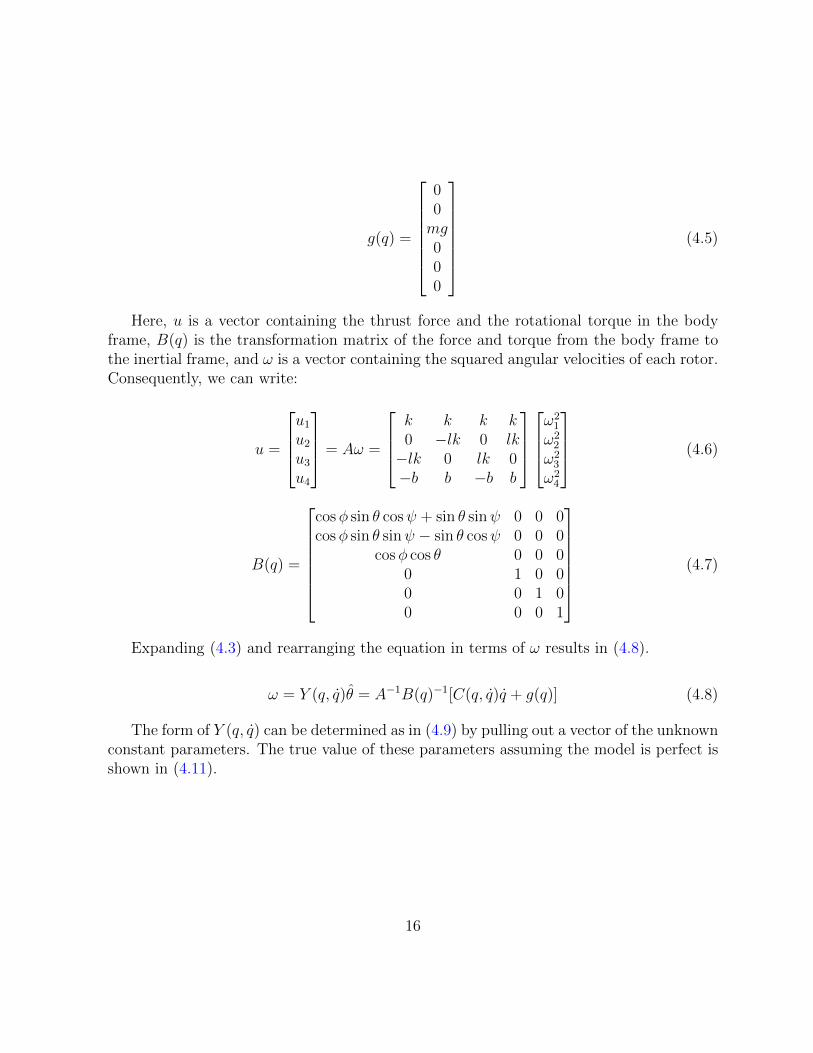
g(q) =

00mg000

(4.5)

Here, u is a vector containing the thrust force and the rotational torque in the bodyframe, B(q) is the transformation matrix of the force and torque from the body frame tothe inertial frame, and ω is a vector containing the squared angular velocities of each rotor.Consequently, we can write:

u =

u1u2u3u4

= Aω =

k k k k0 −lk 0 lk−lk 0 lk 0−b b −b b

ω21

ω22

ω23

ω24

(4.6)

B(q) =

cosφ sin θ cosψ + sin θ sinψ 0 0 0cosφ sin θ sinψ − sin θ cosψ 0 0 0

cosφ cos θ 0 0 00 1 0 00 0 1 00 0 0 1

(4.7)

Expanding (4.3) and rearranging the equation in terms of ω results in (4.8).

ω = Y (q, q)θ = A−1B(q)−1[C(q, q)q + g(q)] (4.8)

The form of Y (q, q) can be determined as in (4.9) by pulling out a vector of the unknownconstant parameters. The true value of these parameters assuming the model is perfect isshown in (4.11).

16

Y (q, q)θ =

a|x|x b|y|y c|z|z c 0 −φψ −φθa|x|x b|y|y c|z|z c −θψ 0 φθ

a|x|x b|y|y c|z|z c 0 φψ −φθa|x|x b|y|y c|z|z c θψ 0 φθ

θ1θ2θ3θ4θ5θ6θ7

(4.9)

d = (cosφ sin θ cosψ+sin θ sinψ)2 +(cosφ sin θ sinψ− sin θ cosψ)2 +(cosφ cos θ)2 (4.10a)

a = (cosφ sin θ cosψ + sin θ sinψ)/d (4.10b)

b = (cosφ sin θ sinψ − sin θ cosψ)/d (4.10c)

c = (cosφ cos θ)/d (4.10d)

θ =

Ax/4kAy/4kAz/4kmg/4k

(Izz − Iyy)/2kl(Ixx − Izz)/2kl(Iyy − Ixx)/2kl

(4.11)

The adaptive controller and parameter update equations are shown in (4.12) and (4.13)respectively. K is the control gain matrix (4.14), TR is the transformation from task spaceto rotor space (4.15), e is the state error, and L is the learning rate. The value of L caneither be a constant or a 4x4 matrix. For simplicity a constant value of one is used.

ω = Y (q, q)θ + TRKe (4.12)

˙θ = LY TTRKe (4.13)

17

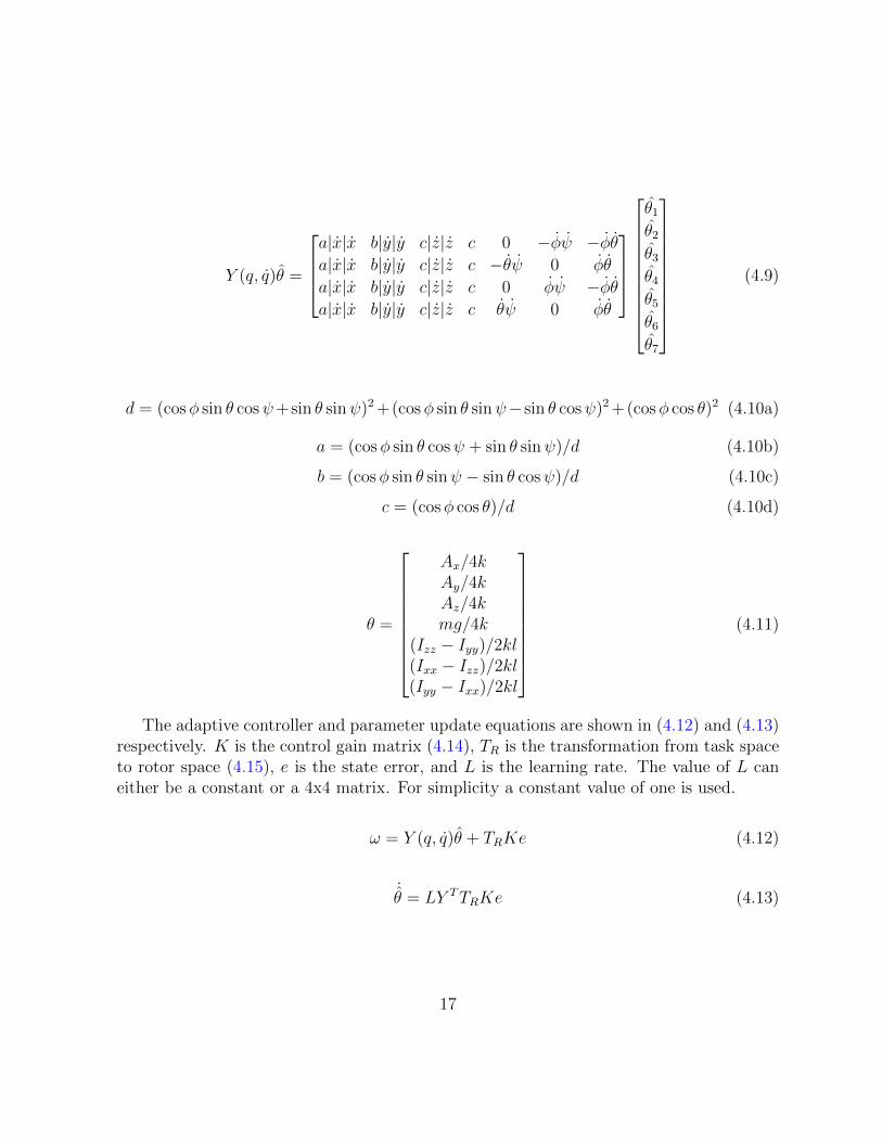
4.2 Controller Implementation

The goal of the controller is to actuate the quadcopter in such a way that it travels to adesired position in a reasonable amount of time. This position is specified as a set of x, y,and z coordinates and a particular yaw direction. The controller is given the state errorof the quadcopter and its target, as well as the current linear and angular velocities of thequadcopter. It needs to use this information to generate a suitable control signal.

The adaptive controller here consists of two parts. The first is a standard PD controllerthat generates a four-dimensional output signal in the space of possible quadcopter motions(task space). The gain matrix that performs this operation can be seen in (4.14). Thissignal is then multiplied by the matrix in (4.15) to transform it into the four dimensionalrotor velocity space, providing the actuation associated with the desired movement com-mands. The design of this matrix depends upon the orientation of the rotor blades to thex and y axes. This transformation matrix assumes that the rotor axes are offset from thex and y axes by 45 degrees as the V-REP model used here.

K =

0 0 k2 0 0 −k4 0 0 0 0 0 00 k1 0 0 −k3 0 −k5 0 0 k7 0 0−k1 0 0 k3 0 0 0 −k5 0 0 k7 0

0 0 0 0 0 0 0 0 −k6 0 0 k8

(4.14)

TR =

1 −1 1 11 −1 −1 −11 1 −1 11 1 1 −1

(4.15)

u =

w2

1

w22

w23

w24

= TRK

xyzxyzφθψ

φ

θ

ψ

(4.16)

18

Translation in the x and y directions is dependent on the states of both x and y aswell as roll and pitch, because a roll in the quadcopter causes a component of thrust to beapplied in the y direction, and a pitch causes a component of thrust to be applied in thex direction. A delicate balance needs to be found between each of the gains in order tocreate a stable, functioning controller. The setpoint for each of the velocities as well as forroll and pitch is zero.

The state error is measured relative to the body frame because most sensors on a realquadcopter would return measurements relative to the sensor device itself, which is locatedon the quadcopter. Absolute measurements could still be obtained with a GPS device, butwould typically be much less accurate and such devices are harder to use for fine-tunedcontrol. Using localized sensors, the state of the quadcopter can be defined relative to itstarget, making the state in the same coordinates as the error.

Here the controller is implemented with a Nengo network, in which a 12-dimensionalensemble representing the state error can be projected to a 4-dimensional ensemble rep-resenting the desired control command. The transformation done through this projectionwill be by the 12x4 PD gain matrix of the controller (4.14). This 4-dimensional ensemble isthen projected to another 4-dimensional ensemble which represents the four desired angu-lar velocities of the quadcopter’s rotors. This projection is done through a transformationby the 4x4 rotor matrix (4.15). This rotor velocity ensemble is connected to a node rep-resenting the physical quadcopter, which in turn feeds back into the state error ensemble.The network diagram is shown in Figure 4.1. The network can be simplified further bymultiplying the gain matrix with the rotor matrix to give a single transformation matrixfrom state error to rotor velocity. This simplified and functionally equivalent network isshown in Figure 4.2. The larger network is used in the remainder of this thesis because itis more explicit regarding how each signal is used, and allows greater flexibility for designimprovements and system debugging.

4.3 Iterations

The first version of the controller uses an adaptive ensemble to influence the task spacecommand. A projection from the adaptive ensemble to the task ensemble is modulatedby the state error undergoing the control transform. The PES learning rule is applied tothis connection, which seeks to build a transformation that minimizes the error comingin from this modulatory connection. The effect is similar to that of the I term in a PIDcontroller, except that it uses all state information to come up with the integral gain, andcan perform nonlinear transforms to accomplish this. Without this adaptive component,

19

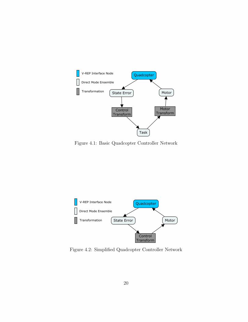
Figure 4.1: Basic Quadcopter Controller Network

Figure 4.2: Simplified Quadcopter Controller Network

20

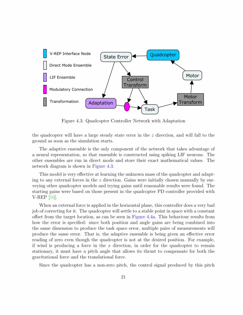
Figure 4.3: Quadcopter Controller Network with Adaptation

the quadcopter will have a large steady state error in the z direction, and will fall to theground as soon as the simulation starts.

The adaptive ensemble is the only component of the network that takes advantage ofa neural representation, so that ensemble is constructed using spiking LIF neurons. Theother ensembles are run in direct mode and store their exact mathematical values. Thenetwork diagram is shown in Figure 4.3.

This model is very effective at learning the unknown mass of the quadcopter and adapt-ing to any external forces in the z direction. Gains were initially chosen manually by sur-veying other quadcopter models and trying gains until reasonable results were found. Thestarting gains were based on those present in the quadcopter PD controller provided withV-REP [10].

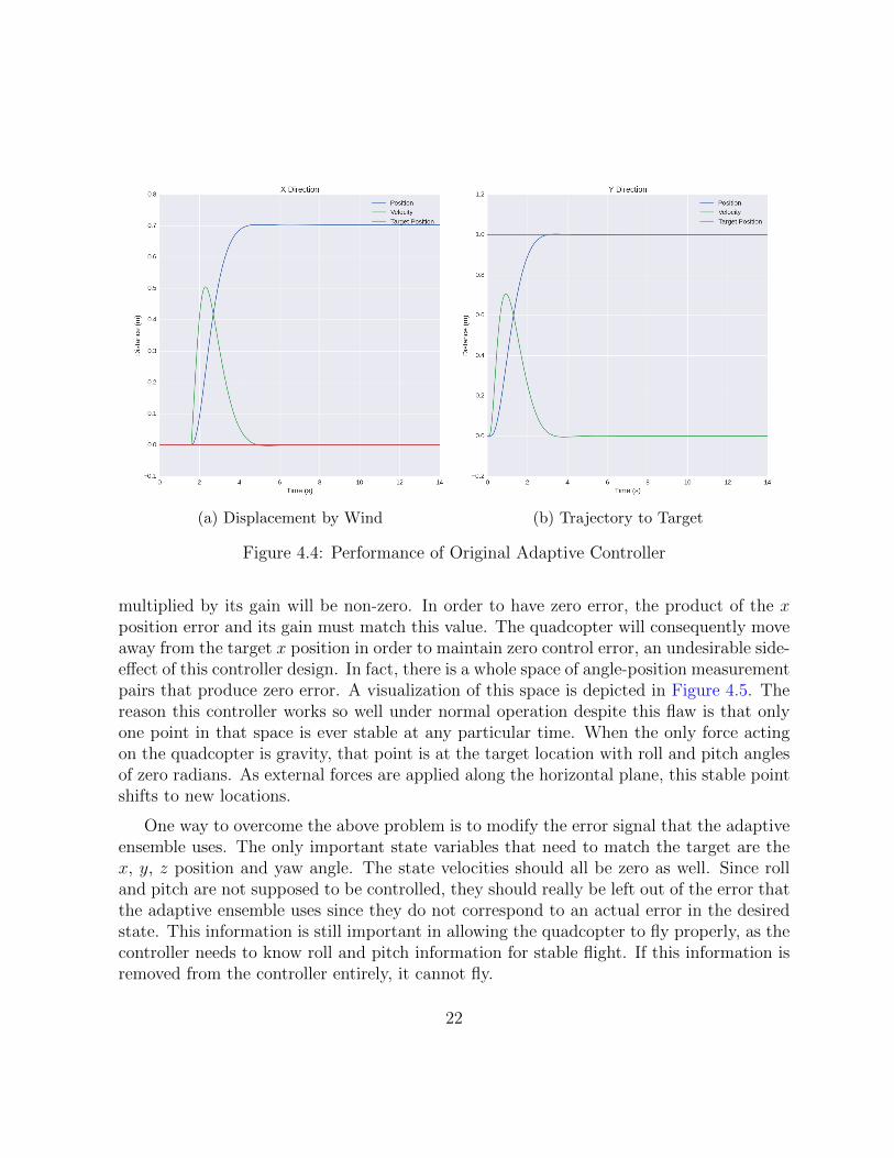
When an external force is applied in the horizontal plane, this controller does a very badjob of correcting for it. The quadcopter will settle to a stable point in space with a constantoffset from the target location, as can be seen in Figure 4.4a. This behaviour results fromhow the error is specified: since both position and angle gains are being combined intothe same dimension to produce the task space error, multiple pairs of measurements willproduce the same error. That is, the adaptive ensemble is being given an effective errorreading of zero even though the quadcopter is not at the desired position. For example,if wind is producing a force in the x direction, in order for the quadcopter to remainstationary, it must have a pitch angle that allows its thrust to compensate for both thegravitational force and the translational force.

Since the quadcopter has a non-zero pitch, the control signal produced by this pitch

21

(a) Displacement by Wind (b) Trajectory to Target

Figure 4.4: Performance of Original Adaptive Controller

multiplied by its gain will be non-zero. In order to have zero error, the product of the xposition error and its gain must match this value. The quadcopter will consequently moveaway from the target x position in order to maintain zero control error, an undesirable side-effect of this controller design. In fact, there is a whole space of angle-position measurementpairs that produce zero error. A visualization of this space is depicted in Figure 4.5. Thereason this controller works so well under normal operation despite this flaw is that onlyone point in that space is ever stable at any particular time. When the only force actingon the quadcopter is gravity, that point is at the target location with roll and pitch anglesof zero radians. As external forces are applied along the horizontal plane, this stable pointshifts to new locations.

One way to overcome the above problem is to modify the error signal that the adaptiveensemble uses. The only important state variables that need to match the target are thex, y, z position and yaw angle. The state velocities should all be zero as well. Since rolland pitch are not supposed to be controlled, they should really be left out of the error thatthe adaptive ensemble uses since they do not correspond to an actual error in the desiredstate. This information is still important in allowing the quadcopter to fly properly, as thecontroller needs to know roll and pitch information for stable flight. If this information isremoved from the controller entirely, it cannot fly.

22

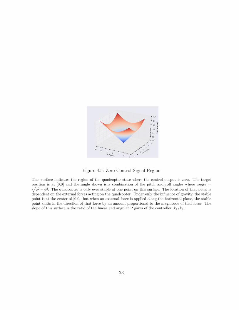
Figure 4.5: Zero Control Signal Region

This surface indicates the region of the quadcopter state where the control output is zero. The targetposition is at [0,0] and the angle shown is a combination of the pitch and roll angles where angle =√φ2 + θ2. The quadcopter is only ever stable at one point on this surface. The location of that point is

dependent on the external forces acting on the quadcopter. Under only the influence of gravity, the stablepoint is at the center of [0,0], but when an external force is applied along the horizontal plane, the stablepoint shifts in the direction of that force by an amount proportional to the magnitude of that force. Theslope of this surface is the ratio of the linear and angular P gains of the controller, k1/k5.

23

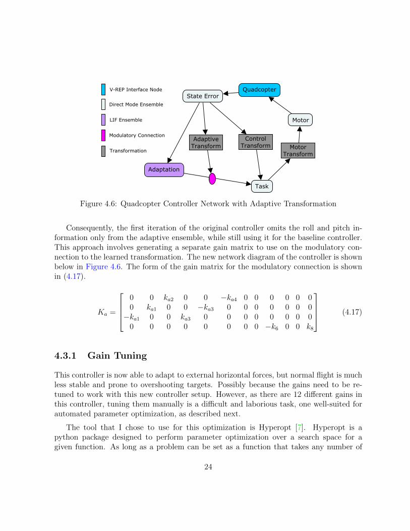
Figure 4.6: Quadcopter Controller Network with Adaptive Transformation

Consequently, the first iteration of the original controller omits the roll and pitch in-formation only from the adaptive ensemble, while still using it for the baseline controller.This approach involves generating a separate gain matrix to use on the modulatory con-nection to the learned transformation. The new network diagram of the controller is shownbelow in Figure 4.6. The form of the gain matrix for the modulatory connection is shownin (4.17).

Ka =

0 0 ka2 0 0 −ka4 0 0 0 0 0 00 ka1 0 0 −ka3 0 0 0 0 0 0 0−ka1 0 0 ka3 0 0 0 0 0 0 0 0

0 0 0 0 0 0 0 0 −k6 0 0 k8

(4.17)

4.3.1 Gain Tuning

This controller is now able to adapt to external horizontal forces, but normal flight is muchless stable and prone to overshooting targets. Possibly because the gains need to be re-tuned to work with this new controller setup. However, as there are 12 different gains inthis controller, tuning them manually is a difficult and laborious task, one well-suited forautomated parameter optimization, as described next.

The tool that I chose to use for this optimization is Hyperopt [7]. Hyperopt is apython package designed to perform parameter optimization over a search space for agiven function. As long as a problem can be set as a function that takes any number of

24

parameters and returns a single error metric to be minimized, that problem can be usedwith Hyperopt. Hyperopt uses a technique known as Sequential Model-Based Optimization(SMBO) for function optimization. SMBO methods are typically used when the goal is tooptimize a function that is costly to evaluate as they invest more time between functionevaluations than other methods, such as conjugate gradient descent, in order to reducethe overall number of evaluations [24, 7]. Since each set of gains to evaluate requires acontroller model to be generated and physics simulation to be run for a fixed amount oftime (on the order of seconds), the evaluations are costly to compute time-wise, leading toSMBO as the preferred choice of optimization method.

4.3.2 Using Hyperopt

In order to use Hyperopt, the controller model must be encapsulated in a function thatreturns a useful metric of how well the controller works. This was done by creating a set oftarget points for the quadcopter to move through over a period of time and an additionalensemble computing a scalar measure of the error of the quadcopter from the target. Thiserror metric was taken to be a weighted Euclidean norm of each of the dimensions of thestate. States that were deemed more important (such as the x, y, and z position) weregiven higher weights in this calculation. States that were less important (such as roll andpitch) were given lower weights. Paired with this error was a status signal of whether thequadcopter should be at the target at a given time or en-route. As the quadcopter cannotbe expected to move instantaneously between targets, it should not be penalized for havingan error when it has just been told to move to a different location. This status signal is setto 0 right after a new target is introduced, and then set to 1 again about the time whenthe quadcopter is expected to have reached the new target. The error at each time stepis multiplied by this status signal before being recorded. The delay in switching back onthe status signal can be used to indicate how important it is for the quadcopter to reachthe target quickly. A longer delay means the optimization will find parameters that allowthe quadcopter to reach the target very precisely with little oscillation, but reaching thetarget could take a long time. A shorter delay will prefer controllers that get to the targetquickly, but may overshoot, have a steady state error, or jitter once they reach the target.

Model creation, running the physics simulator, sending the target commands, stoppingthe physics simulator, and returning the error metric were all encapsulated in a singlePython function. This function was then given to Hyperopt, which ran it many timesand kept track of the parameters used for the best result. There were 3000 evaluations ofdifferent parameter sets, and each run took about 30 seconds to complete. Hyperopt isable to go through a set number of evaluation points in one run, and then pick up where

25

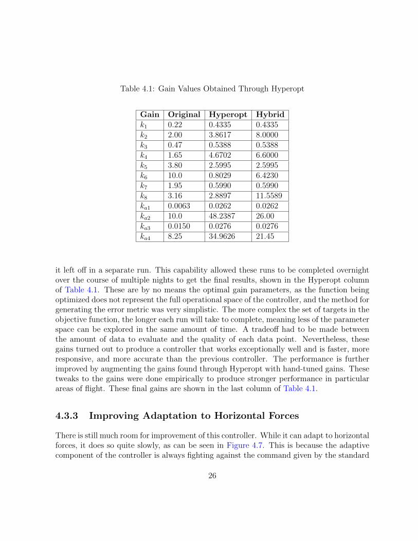
Table 4.1: Gain Values Obtained Through Hyperopt

Gain Original Hyperopt Hybridk1 0.22 0.4335 0.4335k2 2.00 3.8617 8.0000k3 0.47 0.5388 0.5388k4 1.65 4.6702 6.6000k5 3.80 2.5995 2.5995k6 10.0 0.8029 6.4230k7 1.95 0.5990 0.5990k8 3.16 2.8897 11.5589ka1 0.0063 0.0262 0.0262ka2 10.0 48.2387 26.00ka3 0.0150 0.0276 0.0276ka4 8.25 34.9626 21.45

it left off in a separate run. This capability allowed these runs to be completed overnightover the course of multiple nights to get the final results, shown in the Hyperopt columnof Table 4.1. These are by no means the optimal gain parameters, as the function beingoptimized does not represent the full operational space of the controller, and the method forgenerating the error metric was very simplistic. The more complex the set of targets in theobjective function, the longer each run will take to complete, meaning less of the parameterspace can be explored in the same amount of time. A tradeoff had to be made betweenthe amount of data to evaluate and the quality of each data point. Nevertheless, thesegains turned out to produce a controller that works exceptionally well and is faster, moreresponsive, and more accurate than the previous controller. The performance is furtherimproved by augmenting the gains found through Hyperopt with hand-tuned gains. Thesetweaks to the gains were done empirically to produce stronger performance in particularareas of flight. These final gains are shown in the last column of Table 4.1.

4.3.3 Improving Adaptation to Horizontal Forces

There is still much room for improvement of this controller. While it can adapt to horizontalforces, it does so quite slowly, as can be seen in Figure 4.7. This is because the adaptivecomponent of the controller is always fighting against the command given by the standard

26

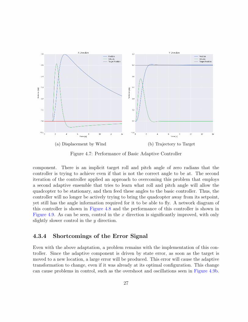
(a) Displacement by Wind (b) Trajectory to Target

Figure 4.7: Performance of Basic Adaptive Controller

component. There is an implicit target roll and pitch angle of zero radians that thecontroller is trying to achieve even if that is not the correct angle to be at. The seconditeration of the controller applied an approach to overcoming this problem that employsa second adaptive ensemble that tries to learn what roll and pitch angle will allow thequadcopter to be stationary, and then feed these angles to the basic controller. Thus, thecontroller will no longer be actively trying to bring the quadcopter away from its setpoint,yet still has the angle information required for it to be able to fly. A network diagram ofthis controller is shown in Figure 4.8 and the performance of this controller is shown inFigure 4.9. As can be seen, control in the x direction is significantly improved, with onlyslightly slower control in the y direction.

4.3.4 Shortcomings of the Error Signal

Even with the above adaptation, a problem remains with the implementation of this con-troller. Since the adaptive component is driven by state error, as soon as the target ismoved to a new location, a large error will be produced. This error will cause the adaptivetransformation to change, even if it was already at its optimal configuration. This changecan cause problems in control, such as the overshoot and oscillations seen in Figure 4.9b.

27

Figure 4.8: Quadcopter Controller Network with Angle Correction

(a) Displacement by Wind (b) Trajectory to Target

Figure 4.9: Performance of Angle Correction Controller

28

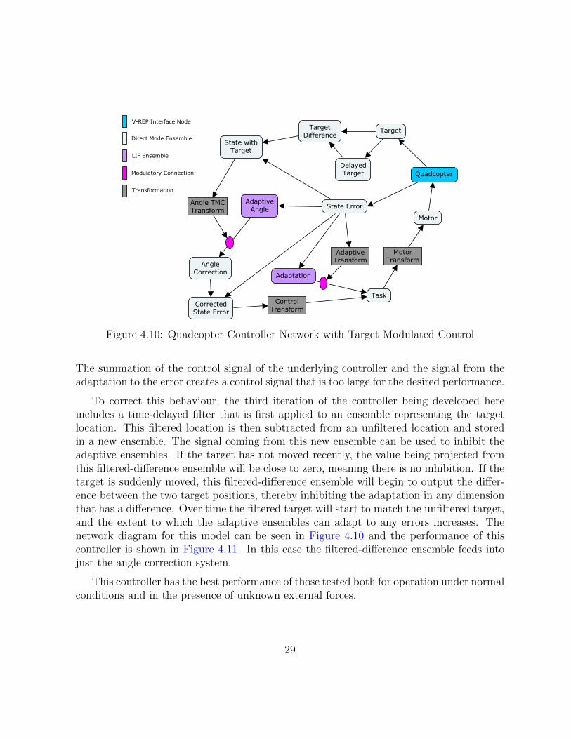
Figure 4.10: Quadcopter Controller Network with Target Modulated Control

The summation of the control signal of the underlying controller and the signal from theadaptation to the error creates a control signal that is too large for the desired performance.

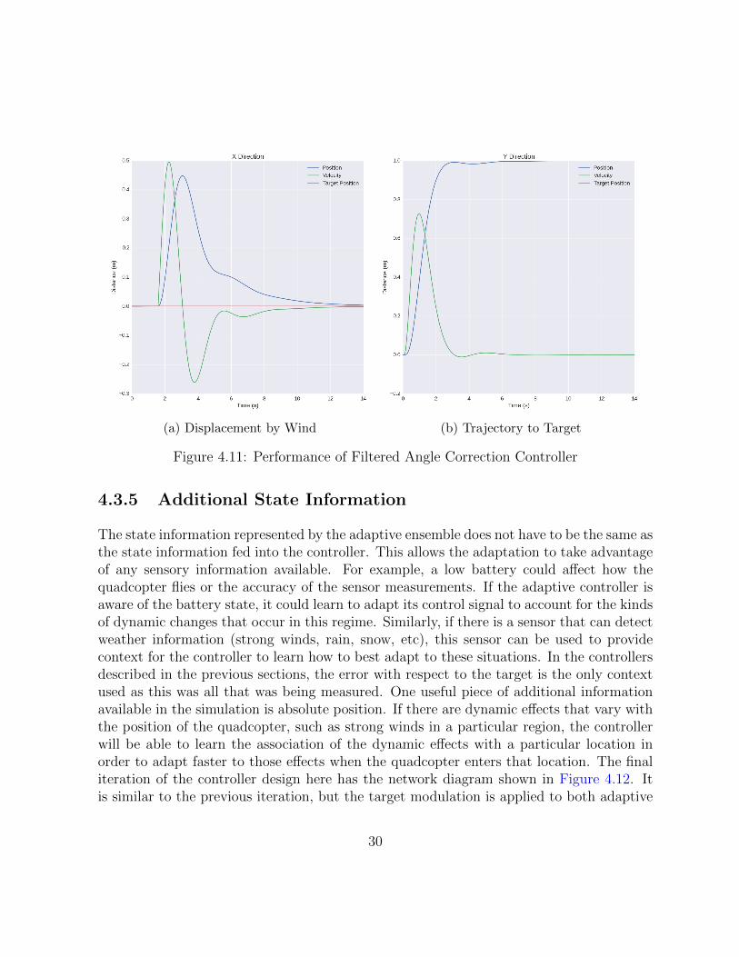
To correct this behaviour, the third iteration of the controller being developed hereincludes a time-delayed filter that is first applied to an ensemble representing the targetlocation. This filtered location is then subtracted from an unfiltered location and storedin a new ensemble. The signal coming from this new ensemble can be used to inhibit theadaptive ensembles. If the target has not moved recently, the value being projected fromthis filtered-difference ensemble will be close to zero, meaning there is no inhibition. If thetarget is suddenly moved, this filtered-difference ensemble will begin to output the differ-ence between the two target positions, thereby inhibiting the adaptation in any dimensionthat has a difference. Over time the filtered target will start to match the unfiltered target,and the extent to which the adaptive ensembles can adapt to any errors increases. Thenetwork diagram for this model can be seen in Figure 4.10 and the performance of thiscontroller is shown in Figure 4.11. In this case the filtered-difference ensemble feeds intojust the angle correction system.

This controller has the best performance of those tested both for operation under normalconditions and in the presence of unknown external forces.

29

(a) Displacement by Wind (b) Trajectory to Target

Figure 4.11: Performance of Filtered Angle Correction Controller

4.3.5 Additional State Information

The state information represented by the adaptive ensemble does not have to be the same asthe state information fed into the controller. This allows the adaptation to take advantageof any sensory information available. For example, a low battery could affect how thequadcopter flies or the accuracy of the sensor measurements. If the adaptive controller isaware of the battery state, it could learn to adapt its control signal to account for the kindsof dynamic changes that occur in this regime. Similarly, if there is a sensor that can detectweather information (strong winds, rain, snow, etc), this sensor can be used to providecontext for the controller to learn how to best adapt to these situations. In the controllersdescribed in the previous sections, the error with respect to the target is the only contextused as this was all that was being measured. One useful piece of additional informationavailable in the simulation is absolute position. If there are dynamic effects that vary withthe position of the quadcopter, such as strong winds in a particular region, the controllerwill be able to learn the association of the dynamic effects with a particular location inorder to adapt faster to those effects when the quadcopter enters that location. The finaliteration of the controller design here has the network diagram shown in Figure 4.12. Itis similar to the previous iteration, but the target modulation is applied to both adaptive

30

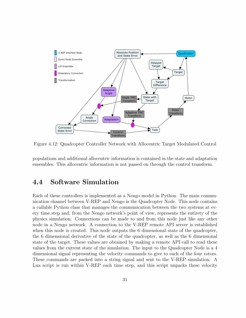
Figure 4.12: Quadcopter Controller Network with Allocentric Target Modulated Control

populations and additional allocentric information is contained in the state and adaptationensembles. This allocentric information is not passed on through the control transform.

4.4 Software Simulation

Each of these controllers is implemented as a Nengo model in Python. The main commu-nication channel between V-REP and Nengo is the Quadcopter Node. This node containsa callable Python class that manages the communication between the two systems at ev-ery time step and, from the Nengo network’s point of view, represents the entirety of thephysics simulation. Connections can be made to and from this node just like any othernode in a Nengo network. A connection to the V-REP remote API server is establishedwhen this node is created. This node outputs the 6 dimensional state of the quadcopter,the 6 dimensional derivative of the state of the quadcopter, as well as the 6 dimensionalstate of the target. These values are obtained by making a remote API call to read thesevalues from the current state of the simulation. The input to the Quadcopter Node is a 4dimensional signal representing the velocity commands to give to each of the four rotors.These commands are packed into a string signal and sent to the V-REP simulation. ALua script is run within V-REP each time step, and this script unpacks these velocity

31

commands. It then issues them to the physical quadcopter model. The physics enginecalculates the appropriate forces and torques that will be applied to the quadcopter as wellas the resulting changes in state (position, velocity, orientation, and angular velocity) afterone time-step. This new state will now be read by the Nengo script in its next time-step.

Nengo is run with a time-step of 1ms, as this is the standard time-step for most modelsand is sufficient for modelling spike timing effects in ensembles of LIF neurons while stillrunning at a reasonable speed on most computer processors. The V-REP simulation onthe other hand is run at a 10ms time-step. Ideally it would also be run at 1ms, but thesimulator has trouble rendering and making calculations that quickly. To account for this,Nengo only communicates with V-REP every 10 of its time-steps. A synchronization triggercommand is also issued every 10 time-steps from Nengo. The V-REP simulation can moveforward only after a trigger is issued, and only by one time-step. Nengo pauses simulationuntil V-REP has completed this time-step. This sequence ensures that the timing of eachsimulation is always synchronized. Some processing overhead is incurred in ensuring thesynchronization of these two systems, but the improved accuracy of the overall simulationjustifies this expense.

32

Chapter 5

Simulations and Results

5.1 Experiments

To get a sense of how well the neural adaptive controller performs, some reference imple-mentations were created to use as benchmarks. Five different non-neural controllers wereused: a standard PD controller, a standard PID controller, an improved PID controller,an improved PID controller with a faster integral gain, and an adaptive controller. Severaliterations of the neural adaptive controller are used in the benchmarking: the basic neuraladaptive controller, the angle corrective controller, the target modulated controller (TMC),and the target modulated controller with allocentric information (TMCA). The controllersused in the benchmarking are listed in Table 5.1

For each non-adaptive reference implementation, a gravity compensation term had tobe calculated and applied to the controllers in order to obtain reasonable performance.The magnitude of this term was determined empirically and is proportional to the massof the quadcopter. The rotor velocity signal is the sum of the gravity compensation termand the output of the controller. The adaptive controllers do not need this extra term asthey are able to learn how to compensate for the effects of gravity very quickly.

5.1.1 Metrics

Three metrics are used to evaluate performance on these tasks. The first is the Root MeanSquared (RMS) error of the difference between the quadcopter’s current state and itstarget state. The quadcopter’s state consists of position, velocity, orientation, and angular

33

Table 5.1: Controller Models

Controller Name DescriptionNeural Adaptive Simple adaptive neural controller. Uses an ensem-

ble of LIF neurons to augment a PD control signalto adapt to an unknown environment. The net-work diagram can be seen in Figure 4.6.

Neural Adaptive Angle Correction Adaptive neural controller with an additionaladaptive neural ensemble for determining stableroll and pitch. The network diagram can be seenin Figure 4.8.

Neural Adaptive TMC The difference between the current target stateand a time delayed target modulates the error sig-nal that drives the learning. The network diagramcan be seen in Figure 4.10.

Neural Adaptive TMCA The same as above, but absolute position and ori-entation information is projected into the adaptiveensembles along with the relative error to the tar-get. The delayed target affects the error signal forboth adaptive ensembles as well. The network di-agram can be seen in Figure 4.12.

Non-Neural Adaptive Adaptive controller using an analytical modelwithout neurons. Derivation shown in section 4.1.

PD Standard PD controller with gravity compensationterm.

PID Standard PID controller with gravity compensa-tion term.

PIDt PID controller where the error signal for the I termis in task space rather than state space. Uses theadaptive transform to calculate this error.

PIDtf PIDt controller with a greater integral gain.

34

velocity. These state variables are combined by computing the length of the resulting12-dimensional error vector to produce a single quantity. This value is calculated at eachtime-step for the duration of the run and then averaged by the number of time-steps in therun. For point to point control this error is sometimes not the most informative becauseas soon as the target point has changed a large error value will be recorded even if thequadcopter is moving optimally towards its target.

The second metric is a modified version of the RMS error designed to take the desiredtrajectory into account. This works by ignoring any error along the direction to the targetas long as the current velocity is also in that direction. It also ignores any error caused bythe velocity in the correct direction as long as the quadcopter is not currently at its target.There are also weights placed on specific types of errors to reflect an increased desire tominimize those errors. For example, errors caused by overshooting the target are weightedmore heavily.

The third metric is the time taken for the quadcopter to reach its target within aparticular tolerance. This metric favours controllers that can reach the target quickly. Thismetric does not worry about overshoot and non-optimal trajectories as long as steady stateis achieved at the target in the end. The particular tolerance chosen for these experimentsis maintaining an RMS error of less than 0.001 for a duration of one second.

The majority of the benchmarks performed in this thesis will report results using thetrajectory RMS error and the time-to-target metric. The RMS metrics were recorded overa 30 second simulation time. The time-to-target trials were also run for a total of 30seconds and a value of 30 is recorded if the quadcopter never reaches its target withintolerance over that duration.

5.1.2 Benchmarks for Simple Environments

A series of simple point-to-point control tasks were used to give an indication of perfor-mance: movement in the vertical direction, movement in the horizontal direction, rotationabout the yaw axis, and horizontal movement into a wind tunnel. These tasks are summa-rized in Table 5.2 below. Each task with translational motion was completed across fourdifferent target distances (every meter from 1m to 4m) and the task with rotational mo-tion was completed across three different target angles (every 45 degrees from 45◦ to 135◦).Experimental results (mean and standard error) obtained from the reference controllersand the neural adaptive controllers are shown for each of these tasks in Figures 5.2 to 5.5.The legend for all of the bar plots in the remainder of this thesis is shown in Figure 5.1.

35

Table 5.2: Benchmark Tasks

Task DescriptionVertical Fly upwards (between one and four meters)Horizontal Fly in the x direction (between one and four me-

ters)Rotation Rotate about the yaw axis (between 45 and 135

degrees)Wind Fly in the y direction (between one and four me-

ters). Enter a wind tunnel after 0.75 meters. Thiswind tunnel exerts a force of 0.6 N in the x direc-tion

Figure 5.1: Controllers used in Benchmarking

36

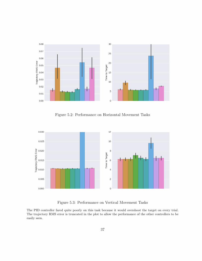
Figure 5.2: Performance on Horizontal Movement Tasks

Figure 5.3: Performance on Vertical Movement Tasks

The PID controller fared quite poorly on this task because it would overshoot the target on every trial.The trajectory RMS error is truncated in the plot to allow the performance of the other controllers to beeasily seen.

37

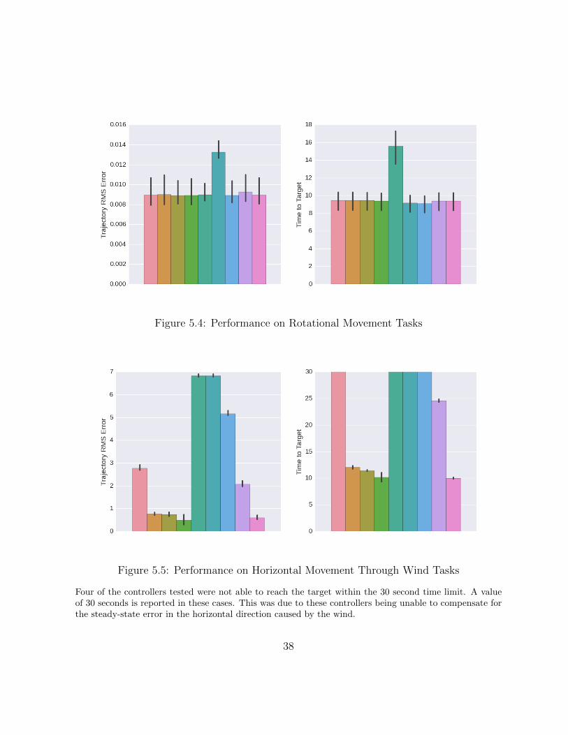
Figure 5.4: Performance on Rotational Movement Tasks

Figure 5.5: Performance on Horizontal Movement Through Wind Tasks

Four of the controllers tested were not able to reach the target within the 30 second time limit. A valueof 30 seconds is reported in these cases. This was due to these controllers being unable to compensate forthe steady-state error in the horizontal direction caused by the wind.

38

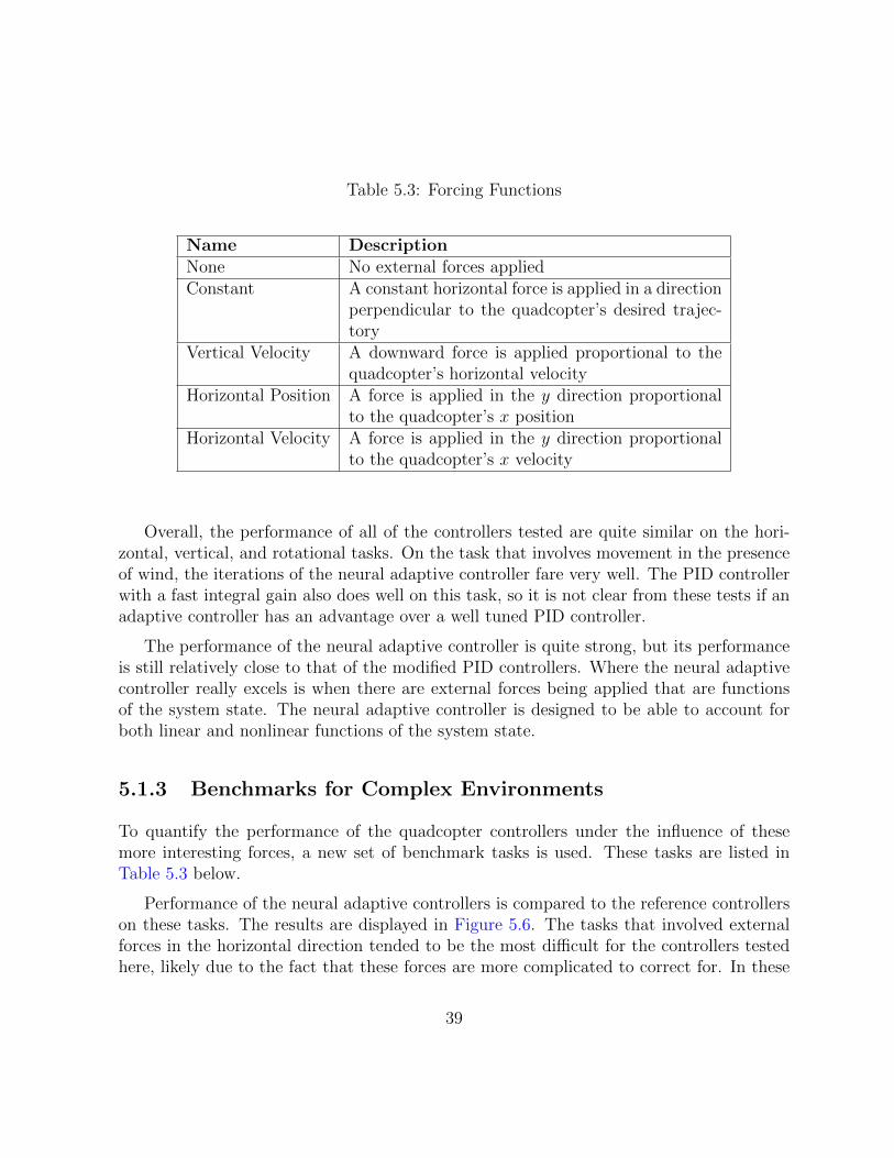
Table 5.3: Forcing Functions

Name DescriptionNone No external forces appliedConstant A constant horizontal force is applied in a direction

perpendicular to the quadcopter’s desired trajec-tory

Vertical Velocity A downward force is applied proportional to thequadcopter’s horizontal velocity

Horizontal Position A force is applied in the y direction proportionalto the quadcopter’s x position

Horizontal Velocity A force is applied in the y direction proportionalto the quadcopter’s x velocity

Overall, the performance of all of the controllers tested are quite similar on the hori-zontal, vertical, and rotational tasks. On the task that involves movement in the presenceof wind, the iterations of the neural adaptive controller fare very well. The PID controllerwith a fast integral gain also does well on this task, so it is not clear from these tests if anadaptive controller has an advantage over a well tuned PID controller.

The performance of the neural adaptive controller is quite strong, but its performanceis still relatively close to that of the modified PID controllers. Where the neural adaptivecontroller really excels is when there are external forces being applied that are functionsof the system state. The neural adaptive controller is designed to be able to account forboth linear and nonlinear functions of the system state.

5.1.3 Benchmarks for Complex Environments

To quantify the performance of the quadcopter controllers under the influence of thesemore interesting forces, a new set of benchmark tasks is used. These tasks are listed inTable 5.3 below.

Performance of the neural adaptive controllers is compared to the reference controllerson these tasks. The results are displayed in Figure 5.6. The tasks that involved externalforces in the horizontal direction tended to be the most difficult for the controllers testedhere, likely due to the fact that these forces are more complicated to correct for. In these

39

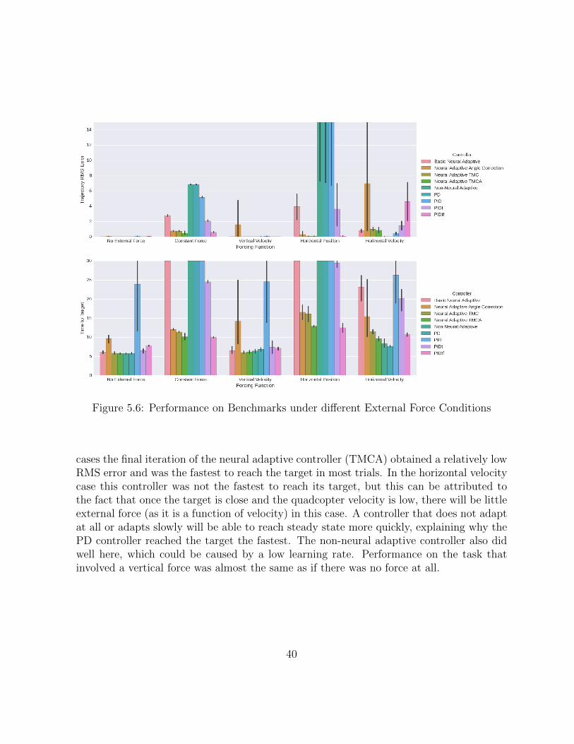
Figure 5.6: Performance on Benchmarks under different External Force Conditions

cases the final iteration of the neural adaptive controller (TMCA) obtained a relatively lowRMS error and was the fastest to reach the target in most trials. In the horizontal velocitycase this controller was not the fastest to reach its target, but this can be attributed tothe fact that once the target is close and the quadcopter velocity is low, there will be littleexternal force (as it is a function of velocity) in this case. A controller that does not adaptat all or adapts slowly will be able to reach steady state more quickly, explaining why thePD controller reached the target the fastest. The non-neural adaptive controller also didwell here, which could be caused by a low learning rate. Performance on the task thatinvolved a vertical force was almost the same as if there was no force at all.

40

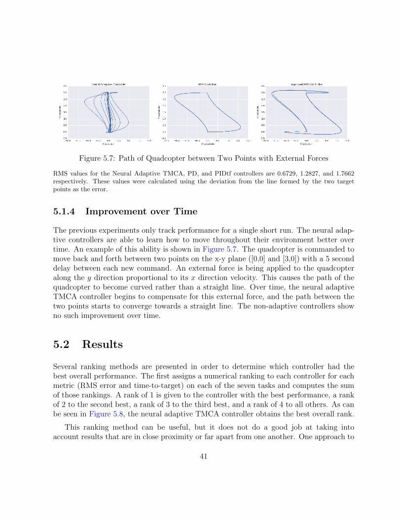
Figure 5.7: Path of Quadcopter between Two Points with External Forces

RMS values for the Neural Adaptive TMCA, PD, and PIDtf controllers are 0.6729, 1.2827, and 1.7662respectively. These values were calculated using the deviation from the line formed by the two targetpoints as the error.

5.1.4 Improvement over Time

The previous experiments only track performance for a single short run. The neural adap-tive controllers are able to learn how to move throughout their environment better overtime. An example of this ability is shown in Figure 5.7. The quadcopter is commanded tomove back and forth between two points on the x-y plane ([0,0] and [3,0]) with a 5 seconddelay between each new command. An external force is being applied to the quadcopteralong the y direction proportional to its x direction velocity. This causes the path of thequadcopter to become curved rather than a straight line. Over time, the neural adaptiveTMCA controller begins to compensate for this external force, and the path between thetwo points starts to converge towards a straight line. The non-adaptive controllers showno such improvement over time.

5.2 Results

Several ranking methods are presented in order to determine which controller had thebest overall performance. The first assigns a numerical ranking to each controller for eachmetric (RMS error and time-to-target) on each of the seven tasks and computes the sumof those rankings. A rank of 1 is given to the controller with the best performance, a rankof 2 to the second best, a rank of 3 to the third best, and a rank of 4 to all others. As canbe seen in Figure 5.8, the neural adaptive TMCA controller obtains the best overall rank.

This ranking method can be useful, but it does not do a good job at taking intoaccount results that are in close proximity or far apart from one another. One approach to

41

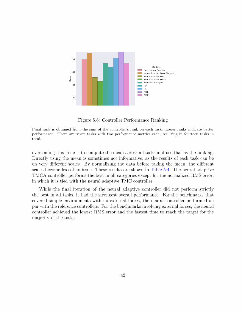
Figure 5.8: Controller Performance Ranking

Final rank is obtained from the sum of the controller’s rank on each task. Lower ranks indicate betterperformance. There are seven tasks with two performance metrics each, resulting in fourteen tasks intotal.

overcoming this issue is to compute the mean across all tasks and use that as the ranking.Directly using the mean is sometimes not informative, as the results of each task can beon very different scales. By normalizing the data before taking the mean, the differentscales become less of an issue. These results are shown in Table 5.4. The neural adaptiveTMCA controller performs the best in all categories except for the normalized RMS error,in which it is tied with the neural adaptive TMC controller.

While the final iteration of the neural adaptive controller did not perform strictlythe best in all tasks, it had the strongest overall performance. For the benchmarks thatcovered simple environments with no external forces, the neural controller performed onpar with the reference controllers. For the benchmarks involving external forces, the neuralcontroller achieved the lowest RMS error and the fastest time to reach the target for themajority of the tasks.

42

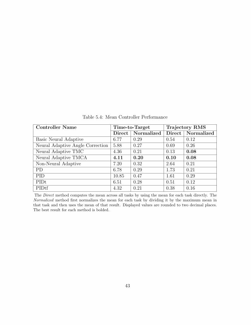
Table 5.4: Mean Controller Performance

Controller Name Time-to-Target Trajectory RMSDirect Normalized Direct Normalized

Basic Neural Adaptive 6.77 0.29 0.54 0.12Neural Adaptive Angle Correction 5.88 0.27 0.69 0.26Neural Adaptive TMC 4.36 0.21 0.13 0.08Neural Adaptive TMCA 4.11 0.20 0.10 0.08Non-Neural Adaptive 7.20 0.32 2.64 0.21PD 6.78 0.29 1.73 0.21PID 10.85 0.47 1.61 0.29PIDt 6.51 0.28 0.51 0.12PIDtf 4.32 0.21 0.38 0.16

The Direct method computes the mean across all tasks by using the mean for each task directly. TheNormalized method first normalizes the mean for each task by dividing it by the maximum mean inthat task and then uses the mean of that result. Displayed values are rounded to two decimal places.The best result for each method is bolded.

43

Chapter 6

Discussion and Future Work

6.1 Contributions

The main contribution of this thesis is an adaptive control system for a quadcopter us-ing simulated biological neurons. This is a proof-of-concept that an ensemble of spikingneurons can be used to improve quadcopter control in the face of uncertain and changingenvironments through a biologically realistic learning mechanism. Using this methodol-ogy, state of the art control can be implemented on the low power and highly parallelarchitecture of neuromorphic hardware.

A second contribution is the integration of the Nengo neural simulation software withthe robotics and physics simulation capacity of V-REP. This union allows complex neu-ral models to be embodied in a physical environment in a straightforward manner. Thevarious tools developed over the course of this thesis work to support the integration ofthe simulated quadcopter with Nengo are general purpose enough to be applied to othersimulated robotic models. These tools include a standard method for opening and closingthe communication channel for the simulators, synchronization of simulation time betweenthe two simulators, an interface for using sensors and actuators from Nengo, and methodfor displaying data from a Nengo network using V-REP’s plotting interface.

6.2 Discussion

While the majority of this work was conducted in an ideal environment with no sensornoise, the neural adaptive controller can still function with noisy measurements. A few

44

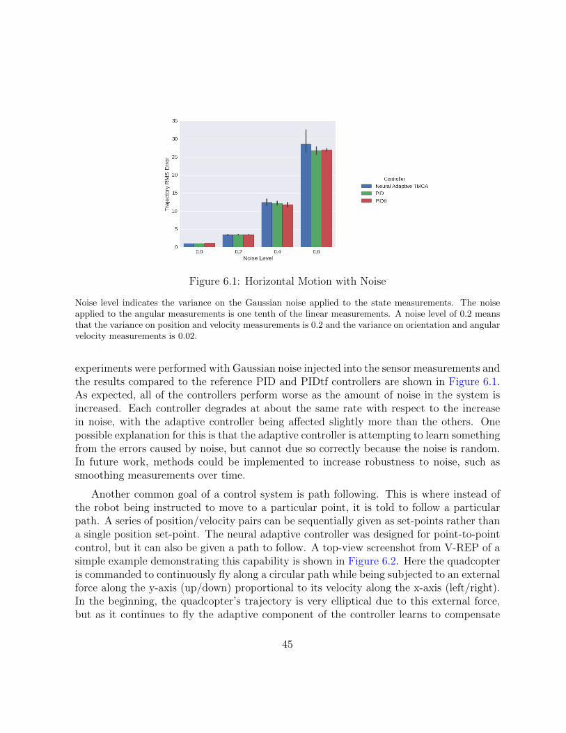
Figure 6.1: Horizontal Motion with Noise

Noise level indicates the variance on the Gaussian noise applied to the state measurements. The noiseapplied to the angular measurements is one tenth of the linear measurements. A noise level of 0.2 meansthat the variance on position and velocity measurements is 0.2 and the variance on orientation and angularvelocity measurements is 0.02.

experiments were performed with Gaussian noise injected into the sensor measurements andthe results compared to the reference PID and PIDtf controllers are shown in Figure 6.1.As expected, all of the controllers perform worse as the amount of noise in the system isincreased. Each controller degrades at about the same rate with respect to the increasein noise, with the adaptive controller being affected slightly more than the others. Onepossible explanation for this is that the adaptive controller is attempting to learn somethingfrom the errors caused by noise, but cannot due so correctly because the noise is random.In future work, methods could be implemented to increase robustness to noise, such assmoothing measurements over time.

Another common goal of a control system is path following. This is where instead ofthe robot being instructed to move to a particular point, it is told to follow a particularpath. A series of position/velocity pairs can be sequentially given as set-points rather thana single position set-point. The neural adaptive controller was designed for point-to-pointcontrol, but it can also be given a path to follow. A top-view screenshot from V-REP of asimple example demonstrating this capability is shown in Figure 6.2. Here the quadcopteris commanded to continuously fly along a circular path while being subjected to an externalforce along the y-axis (up/down) proportional to its velocity along the x-axis (left/right).In the beginning, the quadcopter’s trajectory is very elliptical due to this external force,but as it continues to fly the adaptive component of the controller learns to compensate

45

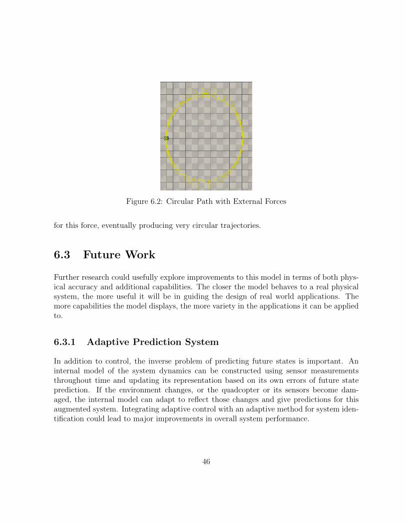
Figure 6.2: Circular Path with External Forces

for this force, eventually producing very circular trajectories.

6.3 Future Work

Further research could usefully explore improvements to this model in terms of both phys-ical accuracy and additional capabilities. The closer the model behaves to a real physicalsystem, the more useful it will be in guiding the design of real world applications. Themore capabilities the model displays, the more variety in the applications it can be appliedto.

6.3.1 Adaptive Prediction System

In addition to control, the inverse problem of predicting future states is important. Aninternal model of the system dynamics can be constructed using sensor measurementsthroughout time and updating its representation based on its own errors of future stateprediction. If the environment changes, or the quadcopter or its sensors become dam-aged, the internal model can adapt to reflect those changes and give predictions for thisaugmented system. Integrating adaptive control with an adaptive method for system iden-tification could lead to major improvements in overall system performance.

46

6.3.2 Integrated Navigation and Planning System

A useful extension of the adaptive controller would be to embed it within a larger navigationand planning system. Currently the quadcopter will only fly in a direct path towards aspecified point, but it would be useful for it to be able to detect obstacles in its pathand calculate a new route to avoid those obstacles. The adaptive ensemble of neurons inthe controller could be set up to be able to recognize certain obstacles and learn to avoidthem in an effective manner. An internal representation of the environment along witha memory for changes in the environment could be used to allow dynamic planning ofoptimal trajectories to a target.

6.3.3 Detailed Modelling

Under special conditions, the dynamics of a quadcopter can change dramatically from theideal model presented in this thesis. One such condition is known as vortex ring state,which can arise when the quadcopter descends too quickly [27]. The quadcopter’s rotorblades may enter the turbulent downwash of the air beneath the craft, causing a severeloss of lift. A vortex forms in a circular ring around the rotors’ path of rotation, bringingturbulent air from beneath the rotors to above them. Increasing the throttle at this pointonly makes the vortex stronger, eventually causing a total loss of lift. This is a dangeroussituation to encounter, so it could be highly beneficial to include some properties of thisstate as well as signs of entering this state (typically wobbling of the craft during descent)in the model. With this extra information, the adaptive controller should have an easiertime learning how to recover from this state and avoid entering it entirely.

Another condition that was not modelled in simulation is blade flapping. This conditionoccurs when the rotor blades undergo translational motion; the advancing blade experiencesa higher tip velocity while the retreating blade experiences a lower tip velocity [3]. Thisdifferential results in an increase in lift in the advancing blade and a decrease in lift in theretreating blade, applying a torque to the rotor disk. The rotor tip path flaps up as theblade advances, and down as the blade retreats to balance the aerodynamic forces. Theadaptive controller is designed to be able to account for external non-linear effects, so thiswould be a good condition to test the controller with in the future.

6.3.4 Realistic Sensors

The current implementation of the simulation is able to directly read the exact state in-formation of the quadcopter. A more realistic scenario would be to use a set of sensors

47

that provide measurements that can be used to estimate the state. Each of these sensorscan have different noise properties and accuracy that can change depending on the situa-tion. The robustness of the adaptive control algorithm to changes in the sensor propertiesand estimation algorithm can be important to characterize when looking into purchasingcomponents to implement the controller on physical hardware.

6.3.5 Running on Physical Hardware

The most practical extension to this work would be to move beyond simulation and runthe control system on physical hardware. Many challenges will arise in this undertaking,including selection of the particular hardware platform, sensors to use, and real-time re-quirements of the control algorithm. Overcoming these challenges to produce an adaptiveneural quadcopter that can interact with the real world will be highly beneficial for explor-ing both practical applications of this work as well as guiding future research direction.

6.4 Conclusion

This project was undertaken to design an adaptive quadcopter controller capable of beingimplemented on neuromorphic hardware and evaluate its performance with respect toconventional controller design methods. The results obtained in simulation are highlypromising and warrant future investigation of more sophisticated neural navigation andplanning systems as well as implementation on physical hardware.

48

APPENDICES

49

Appendix A

Source Code for Thesis Work

All of the source code used to create the quadcopter controllers presented in this thesis isavailable for download at: https://github.com/bjkomer/masters-thesis

Instructions for downloading and installing the necessary software to run the simula-tions and benchmarks are also provided at this link.

50

References

[1] N. H. El-Amary A. I. Hashad A. Y. Elruby, M. M. El-khatib. Dynamic modeling andcontrol of quadrotor vehicle.

[2] Richard Baguley. Best drones 2015.

[3] Moses Bangura and Robert Mahony. Nonlinear dynamic modeling for high perfor-mance control of a quadrotor. In Australasian conference on robotics and automation,pages 1–10, 2012.

[4] Andrew G Barto, Richard S Sutton, and Charles W Anderson. Neuronlike adap-tive elements that can solve difficult learning control problems. Systems, Man andCybernetics, IEEE Transactions on, (5):834–846, 1983.

[5] Trevor Bekolay, James Bergstra, Eric Hunsberger, Travis DeWolf, Terrence C Stewart,Daniel Rasmussen, Xuan Choo, Aaron Russell Voelker, and Chris Eliasmith. Nengo:a python tool for building large-scale functional brain models. Frontiers in neuroin-formatics, 7, 2013.

[6] Trevor Bekolay, Carter Kolbeck, and Chris Eliasmith. Simultaneous unsupervisedand supervised learning of cognitive functions in biologically plausible spiking neuralnetworks. In Proceedings of the 35th annual conference of the cognitive science society,pages 169–174, 2013.

[7] James Bergstra, Dan Yamins, and David D Cox. Hyperopt: A python library foroptimizing the hyperparameters of machine learning algorithms. In Proceedings of the12th Python in Science Conference, pages 13–20, 2013.

[8] Anthony N Burkitt. A review of the integrate-and-fire neuron model: I. homogeneoussynaptic input. Biological cybernetics, 95(1):1–19, 2006.

51

[9] Chien-Chern Cheah, Chao Liu, and Jean-Jacques E Slotine. Adaptive tracking controlfor robots with unknown kinematic and dynamic properties. The International Journalof Robotics Research, 25(3):283–296, 2006.

[10] M. Freese E. Rohmer, S. P. N. Singh. V-rep: a versatile and scalable robot simula-tion framework. In Proc. of The International Conference on Intelligent Robots andSystems (IROS), 2013.

[11] Gilberto Echeverria, Nicolas Lassabe, Arnaud Degroote, and Severin Lemaignan.Modular open robots simulation engine: Morse. In Robotics and Automation (ICRA),2011 IEEE International Conference on, pages 46–51. IEEE, 2011.

[12] Chris Eliasmith. How to build a brain: From function to implementation. Synthese,159(3):373–388, 2007.

[13] Chris Eliasmith. How to build a brain: A neural architecture for biological cognition.Oxford University Press, 2013.

[14] Chris Eliasmith and Charles H Anderson. Neural engineering: Computation, repre-sentation, and dynamics in neurobiological systems. MIT press, 2004.

[15] Elena Garcia, Maria Antonia Jimenez, Pablo Gonzalez De Santos, and Manuel Ar-mada. The evolution of robotics research. Robotics & Automation Magazine, IEEE,14(1):90–103, 2007.

[16] Andrew Gibiansky. Quadcopter dynamics, simulation, and control, 2012.

[17] Sree Harsha, Balaji, and Divya Kamath. Quadcopter, 2014.

[18] Leslie A Hart. How the brain works: A new understanding of human learning, emotion,and thinking. Basic Books, 1975.

[19] Jennifer Hasler and Bo Marr. Finding a roadmap to achieve large neuromorphichardware systems. Frontiers in neuroscience, 7, 2013.

[20] NG Hockstein, CG Gourin, RA Faust, and DJ Terris. A history of robots: fromscience fiction to surgical robotics. Journal of robotic surgery, 1(2):113–118, 2007.

[21] Nathan Koenig and Andrew Howard. Design and use paradigms for gazebo, an open-source multi-robot simulator. In Intelligent Robots and Systems, 2004.(IROS 2004).Proceedings. 2004 IEEE/RSJ International Conference on, volume 3, pages 2149–2154. IEEE, 2004.

52

[22] Gerard Lacey and Kenneth M Dawson-Howe. The application of robotics to a mobilityaid for the elderly blind. Robotics and Autonomous Systems, 23(4):245–252, 1998.

[23] Teppo Luukkonen. Modelling and control of quadcopter. Independent research projectin applied mathematics, Espoo, 2011.

[24] Jonas Mockus, Vytautas Tiesis, and Antanas Zilinskas. The application of bayesianmethods for seeking the extremum. Towards Global Optimization, 2(117-129):2, 1978.

[25] Illah R Nourbakhsh, Katia Sycara, Mary Koes, Mark Yong, Michael Lewis, and SteveBurion. Human-robot teaming for search and rescue. Pervasive Computing, IEEE,4(1):72–79, 2005.

[26] Robert M Sanner and Jean-Jacques E Slotine. Gaussian networks for direct adaptivecontrol. Neural Networks, IEEE Transactions on, 3(6):837–863, 1992.

[27] Quadcopter Flight School. Vortex ring state (the wobble of death), 2014.

[28] Jean-Jacques E Slotine and Weiping Li. On the adaptive control of robot manipulators.The international journal of robotics research, 6(3):49–59, 1987.

[29] Jean-Jacques E Slotine, Weiping Li, et al. Applied nonlinear control, volume 199.Prentice-hall Englewood Cliffs, NJ, 1991.

[30] Terrence C Stewart, Trevor Bekolay, and Chris Eliasmith. Neural representations ofcompositional structures: Representing and manipulating vector spaces with spikingneurons. Connection Science, 23(2):145–153, 2011.

53