Ubiquitous Pattern Matching and Its Applications(Biology, Security, Multimedia)

W. Szpankowskiy

Department of Computer SciencePurdue University

W. Lafayette, IN 47907

May 16, 2003

This research is supported by NSF and NIH.

yJoint work with P. Flajolet, A. Grama, R. Gwadera, M. Regnier, B. Vallee.

Outline of the Talk

1. Pattern Matching Problems

String Matching

Subsequence Matching (Hidden Words)

Self-Repetitive Pattern Matching

2. Biology – String Matching

Analysis (Languages and Generating Functions)

Finding Weak Signals and Artifacts in DNA

3. Information Security – Subsequence Matching

Some Theory (De Bruijn Automaton)

Reliable Threshold in Intrusion Detection

4. Multimedia Compression — Self-Repetitive Matching

Theoretical Foundation (Renyi’s Entropy)

Data Structures and Algorithms

Video Compression (Demo)

Pattern Matching

Let W and T be (set of) strings generated over a finite alphabet A.

We call W the pattern and T the text. The text T is of length n and isgenerated by a probabilistic source.

We shall write

Tn

m = Tm : : : Tn:

The pattern W can be a single stringW = w1 : : : wm; wi 2 A

or a set of strings

W = fW1; : : : ;Wdg

withWi 2 Ami being a set of strings of length mi.

Basic Parameters

Two basic questions are:

how many times W occurs in T ,

how long one has to wait until W occurs in T .

The following quantities are of interest:

On(W) — the number of times W occurs in T :

On(W) = #fi : T iim+1 =W; m i ng:

WW — the first timeW occurs in T :

WW := minfn : T nnm+1 =Wg:

Relationship:

WW > n , On(W) = 0:

Various Pattern Matching

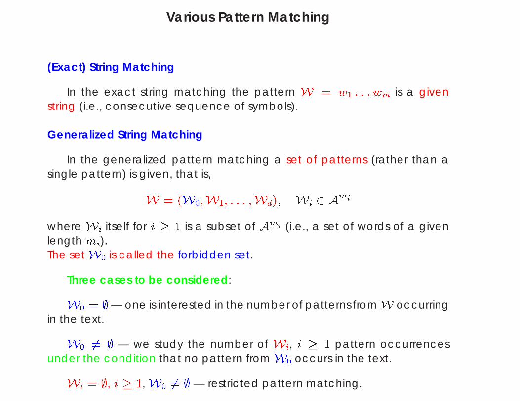
(Exact) String Matching

In the exact string matching the pattern W = w1 : : : wm is a givenstring (i.e., consecutive sequence of symbols).

Generalized String Matching

In the generalized pattern matching a set of patterns (rather than asingle pattern) is given, that is,

W = (W0;W1; : : : ;Wd); Wi 2 Ami

where Wi itself for i 1 is a subset of Ami (i.e., a set of words of a givenlength mi).The set W0 is called the forbidden set.

Three cases to be considered:

W0 = ;— one is interested in the number of patterns fromW occurringin the text.

W0 6= ; — we study the number of Wi, i 1 pattern occurrencesunder the condition that no pattern from W0 occurs in the text.

Wi = ;, i 1, W0 6= ; — restricted pattern matching.

Pattern Matching Problems

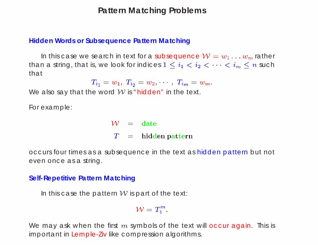
Hidden Words or Subsequence Pattern Matching

In this case we search in text for a subsequence W = w1 : : : wm ratherthan a string, that is, we look for indices 1 i1 < i2 < < im n suchthat

Ti1 = w1; Ti2 = w2; ; Tim = wm:

We also say that the word W is “hidden” in the text.

For example:W = date

T = hidden pattern

occurs four times as a subsequence in the text as hidden pattern but noteven once as a string.

Self-Repetitive Pattern Matching

In this case the patternW is part of the text:

W = Tm

1 :

We may ask when the first m symbols of the text will occur again. This isimportant in Lemple-Ziv like compression algorithms.

Example

Let T = bababababb, andW = abab.

W occurs exactly three times as a string at positions f2; 4; 6g

babab| z ababb:

If W = fabab; babbg, then W occurs four times.

bababababb:

W = abab occurs many times as a subsequence.Here is one subsequence occurrence:

bababababb:

W occurs first time at position 2, i.e., WW = 2:

bababababb:

W = T1T2T3 = bab occurs again (repeats itself) at position 5

bababababb:

Probabilistic Sources

Throughout the talk I will assume that the text is generated by a randomsource.

Memoryless SourceThe text is a realization of an independently, identically distributedsequence of random variables (i.i.d.), such that a symbol s 2 A occurswith probability P (s).

Markovian SourceThe text is a realization of a stationary Markov sequence of order K, thatis, probability of the next symbol occurrence depends on K previoussymbols.

Basic Thrust of our Approach

When searching for over-represented or under-represented patterns we must assure that such apattern is not generated by randomness itself (toavoid too many false positives).

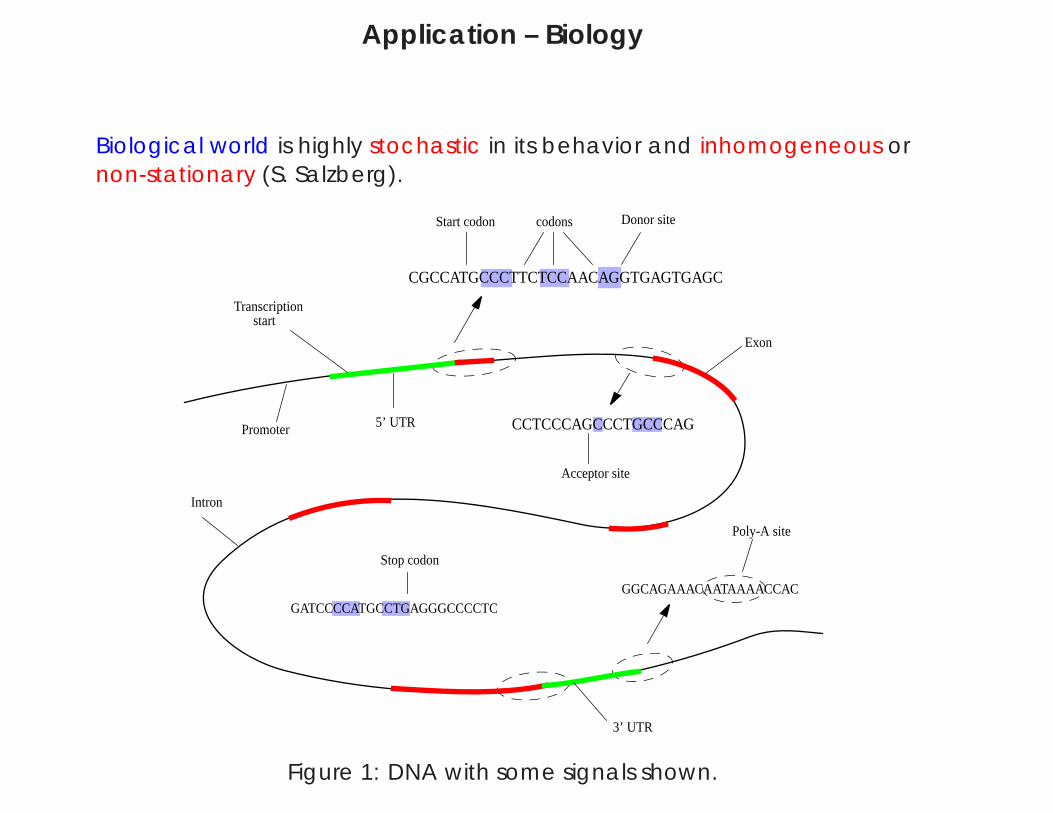
Application – Biology

Biological world is highly stochastic in its behavior and inhomogeneous ornon-stationary (S. Salzberg).

Start codon codons Donor site

CGCCATGCCCTTCTCCAACAGGTGAGTGAGC

Transcription start

Exon

Promoter 5’ UTR CCTCCCAGCCCTGCCCAG

Acceptor site

Intron

Stop codon

GATCCCCATGCCTGAGGGCCCCTCGGCAGAAACAATAAAACCAC

Poly-A site

3’ UTR

Figure 1: DNA with some signals shown.

Some Observations

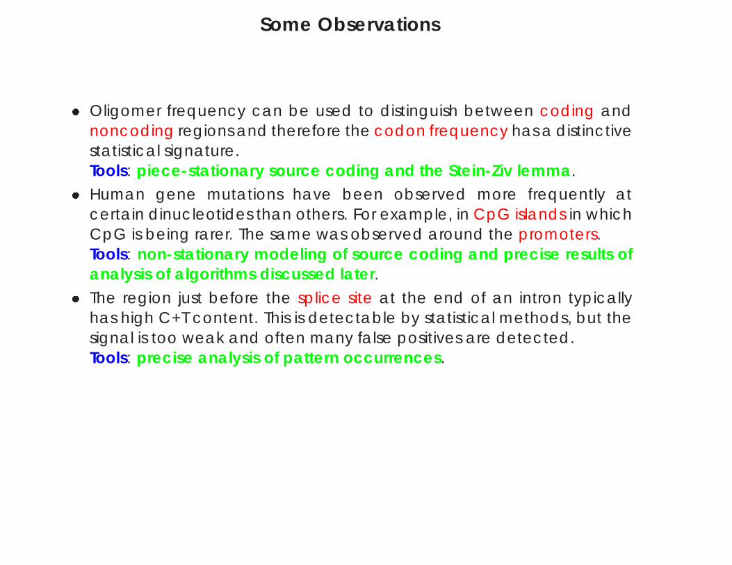
Oligomer frequency can be used to distinguish between coding andnoncoding regions and therefore the codon frequency has a distinctivestatistical signature.Tools: piece-stationary source coding and the Stein-Ziv lemma.

Human gene mutations have been observed more frequently atcertain dinucleotides than others. For example, in CpG islands in whichCpG is being rarer. The same was observed around the promoters.Tools: non-stationary modeling of source coding and precise results ofanalysis of algorithms discussed later.

The region just before the splice site at the end of an intron typicallyhas high C+T content. This is detectable by statistical methods, but thesignal is too weak and often many false positives are detected.Tools: precise analysis of pattern occurrences.

Z Score vs p-values

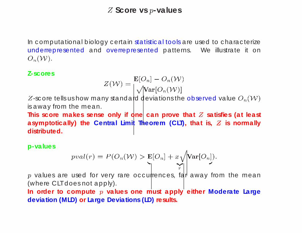
In computational biology certain statistical tools are used to characterizeunderrepresented and overrepresented patterns. We illustrate it on

On(W).

Z-scores

Z(W) =

E[On]On(W)pVar[On(W)]

Z-score tells us how many standard deviations the observed value On(W)

is away from the mean.This score makes sense only if one can prove that Z satisfies (at leastasymptotically) the Central Limit Theorem (CLT), that is, Z is normallydistributed.

p-values

pval(r) = P (On(W) > E[On] + xq

Var[On]| z

r

):

p values are used for very rare occurrences, far away from the mean(where CLT does not apply).In order to compute p values one must apply either Moderate Largedeviation (MLD) or Large Deviations (LD) results.

CLT vs LD

P On µ xσ+>( ) 1

2π---------- e

t2 2⁄

–td

x

∞

∫=1x---e

x2 2⁄

–∼1

x-------e

λx–∼

pval r( ) P On r>( )=

ZE On( ) On–

var On[ ]------------------------------=

CLT MLD LD

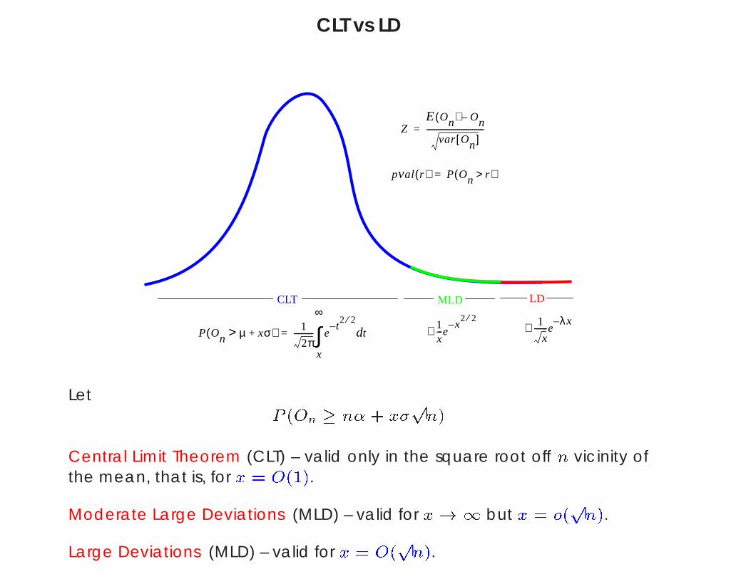
Let

P (On n+ xp

n)

Central Limit Theorem (CLT) – valid only in the square root off n vicinity ofthe mean, that is, for x = O(1).

Moderate Large Deviations (MLD) – valid for x!1 but x = o(p

n).

Large Deviations (MLD) – valid for x = O(p

n).

Z-scores and p values for A.thaliana

Table 1: Z score vs p-value of tandem repeats in A.thaliana.

Oligomer Obs. p-val Z-sc.(large dev.)

AATTGGCGG 2 8:059 104 48.71

TTTGTACCA 3 4:350 105 22.96ACGGTTCAC 3 2:265 106 55.49

AAGACGGTT 3 2:186 106 48.95

ACGACGCTT 4 1:604 109 74.01ACGCTTGG 4 5:374 1010 84.93

GAGAAGACG 5 0:687 1014 151.10

Remark: p values were computed using large deviations results of Regnierand S. (1998), and Denise and Regnier (2001) as we discuss below.

Some Theory

Here is an incomplete list of results on string pattern matching (given apattern W find statistics of its occurrences):

Feller (1968),

Guibas and Odlyzko (1978, 1981),

Prum, Rodolphe, and Turckheim (1995) – Markovian model, limitingdistribution.

Regnier & W.S. (1997,1998) – exact and approximate occurrences(memoryless and Markov models).

P. Nicodeme, Salvy, & P. Flajolet (1999) – regular expressions.

E. Bender and F. Kochman (1993) – general pattern matching.

Languages and Generating Functions

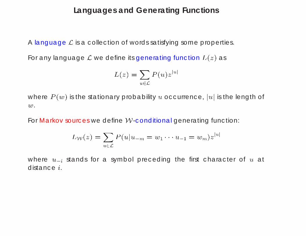
A language L is a collection of words satisfying some properties.

For any language L we define its generating function L(z) as

L(z) =X

u2LP (u)zjuj

where P (w) is the stationary probability u occurrence, juj is the length of

w.

For Markov sources we defineW-conditional generating function:

LW(z) =X

u2LP (ujum = w1 u1 = wm)zjuj

where ui stands for a symbol preceding the first character of u atdistance i.

Autocorrelation Set and Polynomial

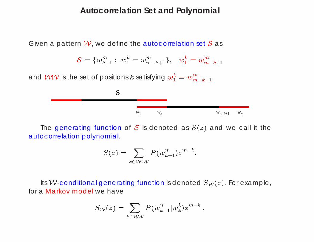
Given a patternW , we define the autocorrelation set S as:

S = fwmk+1 : wk

1 = wmmk+1g; wk1 = wmmk+1

and WW is the set of positions k satisfying wk1 = wmmk+1.

w1 wk wm-k+1 wm

S

The generating function of S is denoted as S(z) and we call it theautocorrelation polynomial.

S(z) =

Xk2W!W

P (wmk+1)zmk:

ItsW-conditional generating function is denoted SW(z). For example,for a Markov model we have

SW(z) =

Xk2WW

P (wmk+1jwkk)zmk :

Example

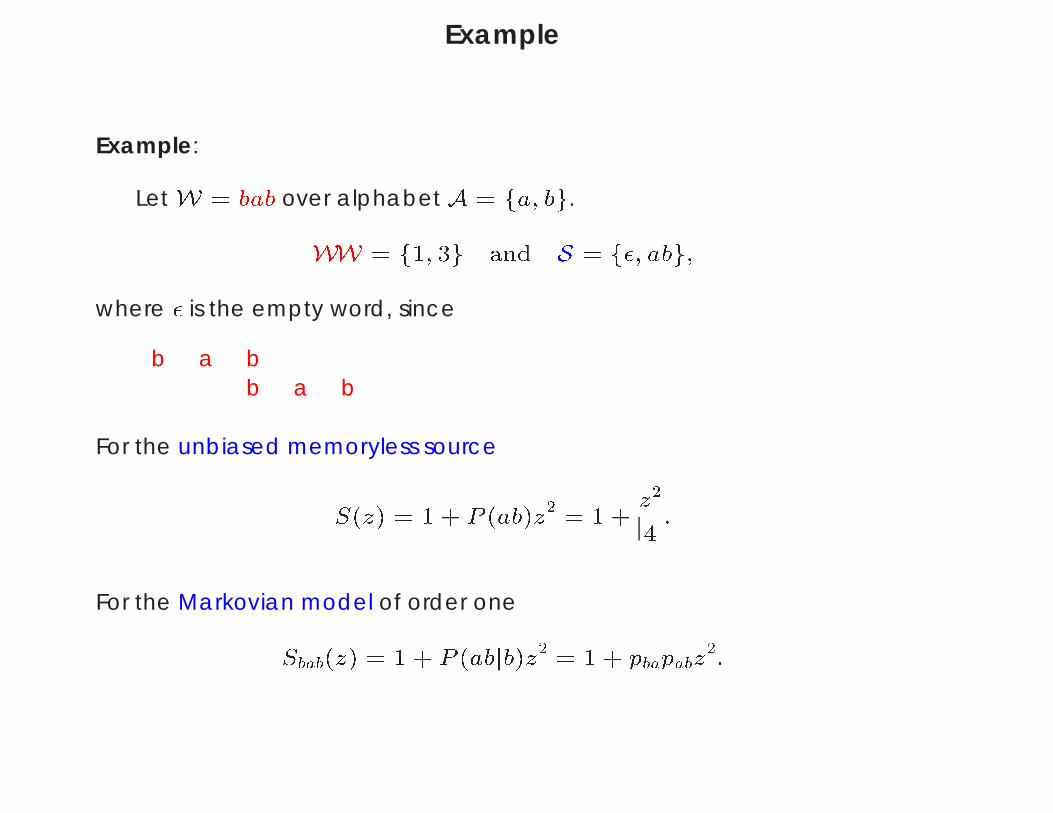
Example:

Let W = bab over alphabetA = fa; bg.

WW = f1; 3g and S = f; abg;

where is the empty word, since

b a bb a b

For the unbiased memoryless source

S(z) = 1 + P (ab)z2= 1 +z2

4:

For the Markovian model of order one

Sbab(z) = 1 + P (abjb)z2 = 1 + pbapabz2:

Language Tr

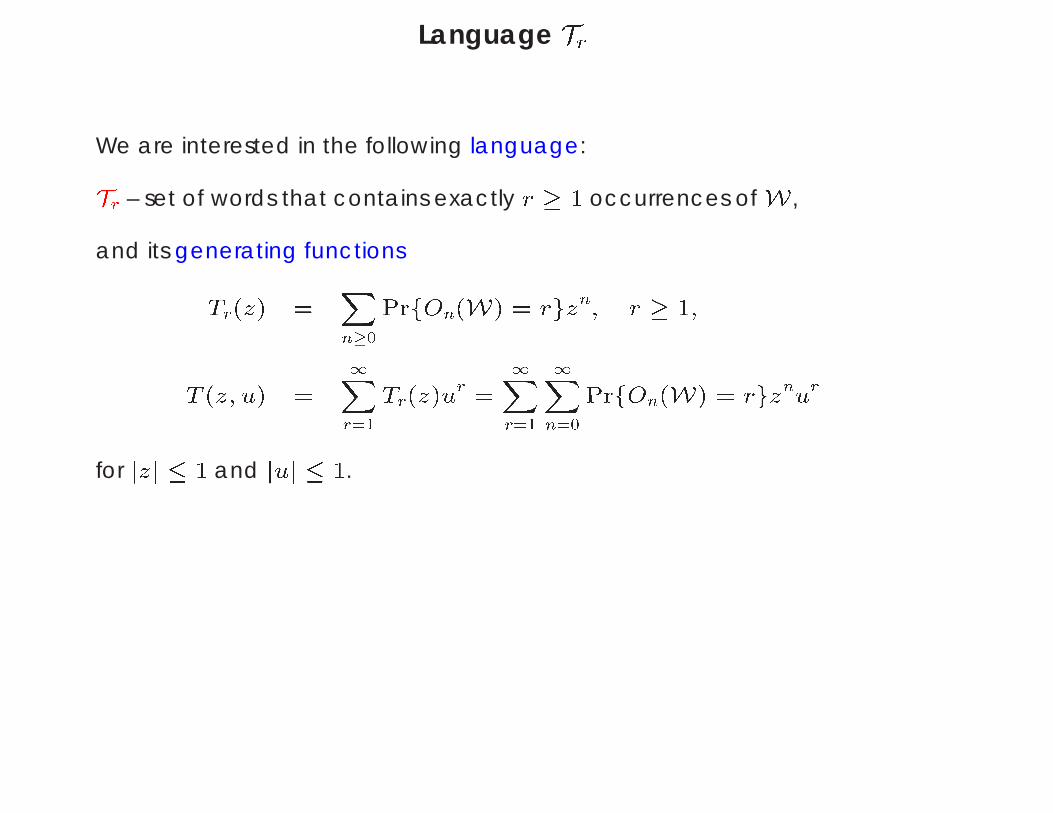
We are interested in the following language:

Tr – set of words that contains exactly r 1 occurrences of W ,

and its generating functions

Tr(z) =

Xn0

PrfOn(W) = rgzn; r 1;

T (z; u) =

1Xr=1Tr(z)ur =

1Xr=1

1Xn=0PrfOn(W) = rgznur

for jzj 1 and juj 1.

More Languages

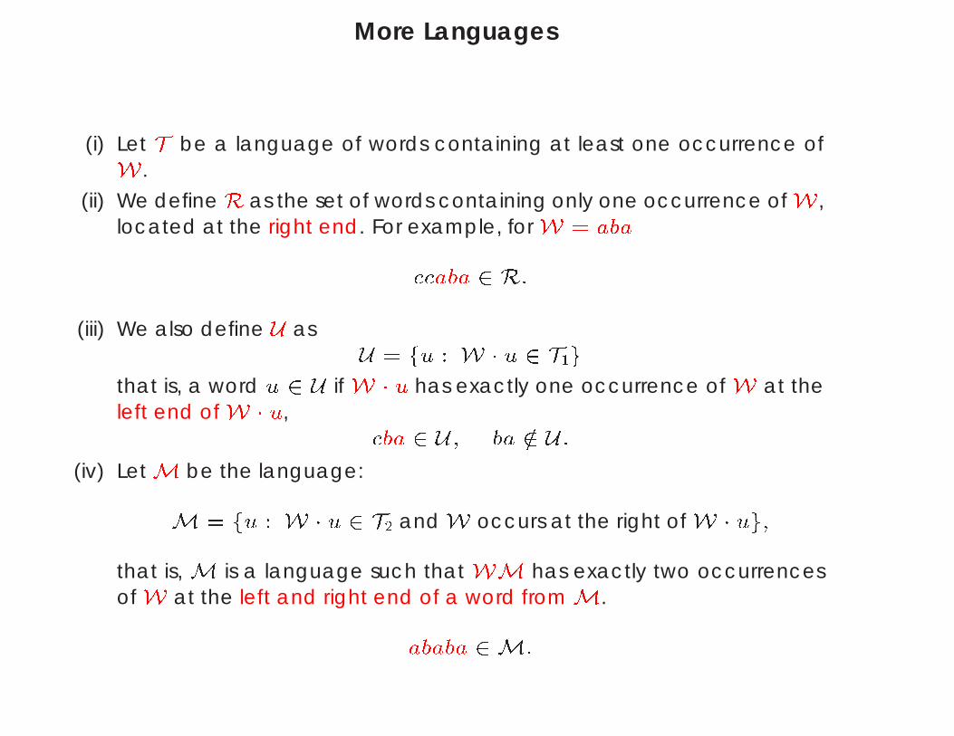
(i) Let T be a language of words containing at least one occurrence of

W .

(ii) We defineR as the set of words containing only one occurrence ofW ,located at the right end. For example, for W = aba

ccaba 2 R:

(iii) We also define U asU = fu : W u 2 T1g

that is, a word u 2 U if W u has exactly one occurrence of W at theleft end ofW u,

cba 2 U ; ba =2 U :

(iv) Let M be the language:

M = fu : W u 2 T2 andW occurs at the right of W ug;

that is, M is a language such that WM has exactly two occurrencesofW at the left and right end of a word from M.

ababa 2 M:

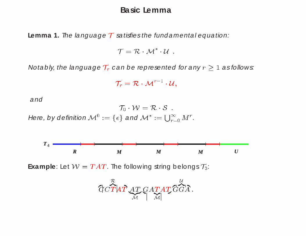
Basic Lemma

Lemma 1. The language T satisfies the fundamental equation:

T = R M U :

Notably, the language Tr can be represented for any r 1 as follows:

Tr = R Mr1 U ;

and

T0 W = R S :

Here, by definitionM0 := fg andM :=S1

r=0Mr.

R M M M UT4

Example: Let W = TAT . The following string belongs T3:

Rz |

CCTAT AT|zM

GATAT| z M

Uz | GGA :

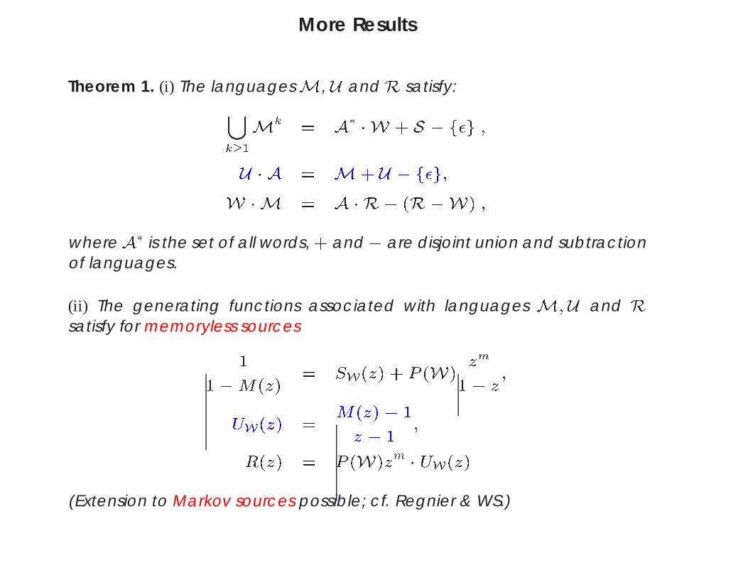
More Results

Theorem 1. (i) The languagesM, U andR satisfy:

[k1Mk

= A W + S fg ;

U A = M+ U fg;

W M = A R (RW) ;

whereA is the set of all words, + and are disjoint union and subtractionof languages.

(ii) The generating functions associated with languages M;U and R

satisfy for memoryless sources

1

1M(z)

= SW(z) + P (W)zm

1 z;

UW(z) =

M(z) 1

z 1

;

R(z) = P (W)zm UW(z)

(Extension to Markov sources possible; cf. Regnier & WS.)

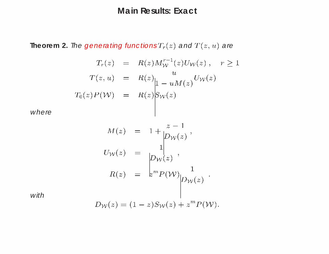
Main Results: Exact

Theorem 2. The generating functions Tr(z) and T (z; u) are

Tr(z) = R(z)Mr1

W (z)UW(z) ; r 1

T (z; u) = R(z)

u

1 uM(z)UW(z)

T0(z)P (W) = R(z)SW(z)

whereM(z) = 1 +

z 1

DW(z);

UW(z) =

1

DW(z);

R(z) = zmP (W)

1

DW(z):

with

DW(z) = (1 z)SW(z) + zmP (W):

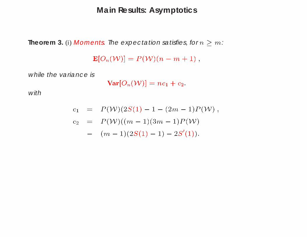
Main Results: Asymptotics

Theorem 3. (i) Moments. The expectation satisfies, for n m:

E[On(W)] = P (W)(n m+ 1) ;

while the variance is

Var[On(W)] = nc1 + c2:

with

c1 = P (W)(2S(1) 1 (2m 1)P (W) ;

c2 = P (W)((m 1)(3m 1)P (W)

(m 1)(2S(1) 1) 2S0(1)):

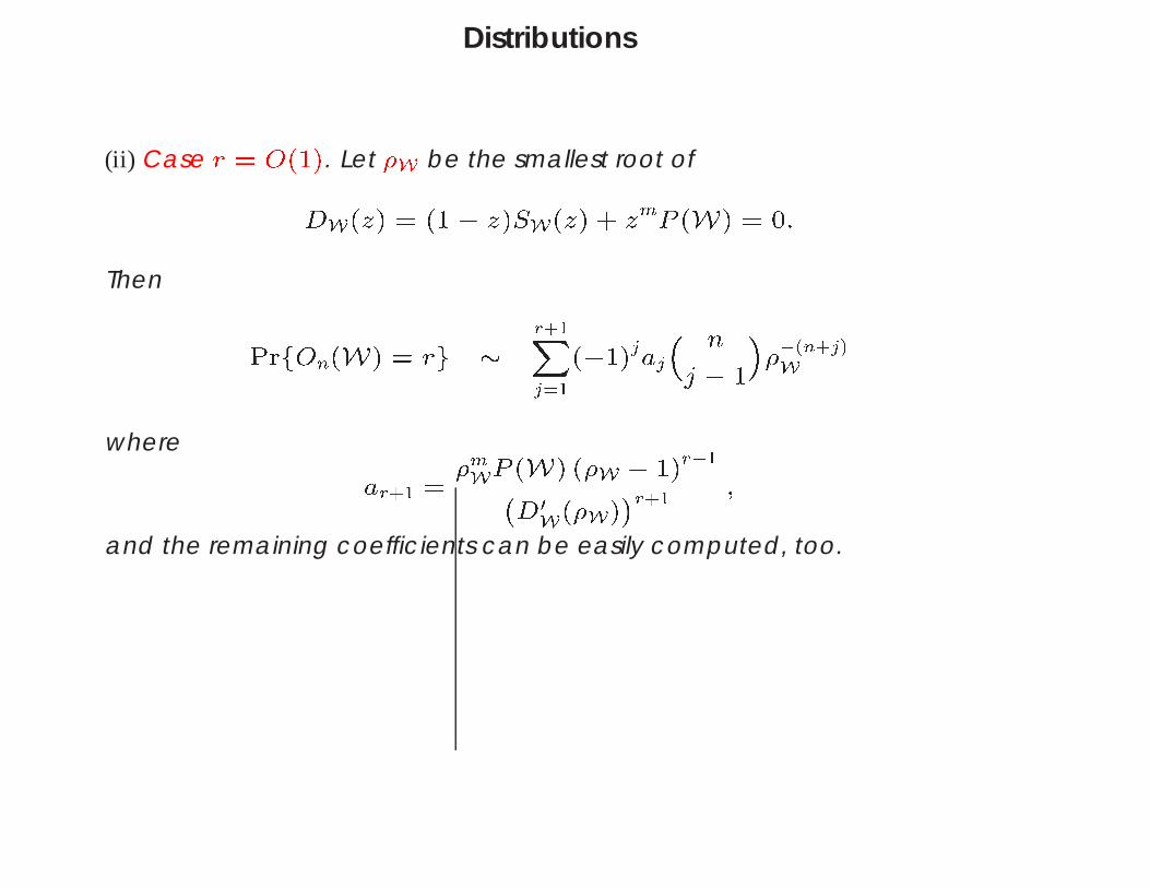
Distributions

(ii) Case r = O(1). Let W be the smallest root of

DW(z) = (1 z)SW(z) + zmP (W) = 0:

Then

PrfOn(W) = rg

r+1Xj=1(1)jaj n

j 1

(n+j)

W

where

ar+1 =

mWP (W) (W 1)r1D0W(W)r+1 ;

and the remaining coefficients can be easily computed, too.

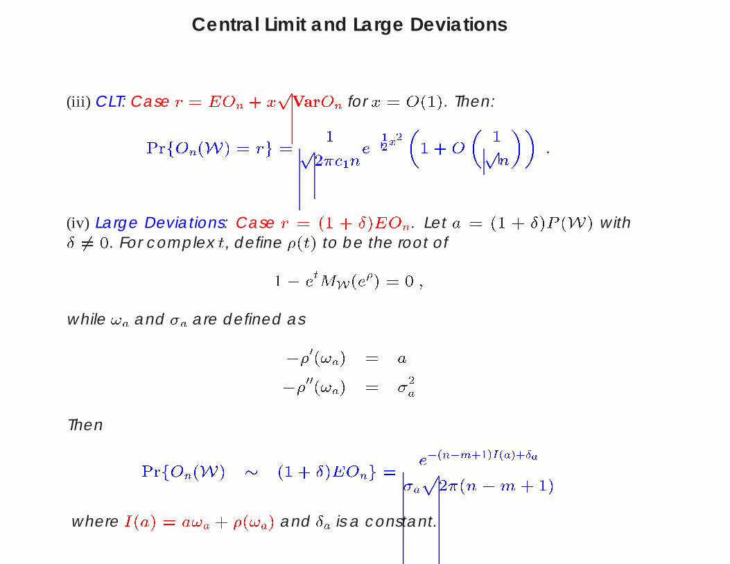
Central Limit and Large Deviations

(iii) CLT: Case r = EOn + xp

VarOn for x = O(1). Then:

PrfOn(W) = rg = 1p2c1ne12x2

1 +O

1pn

:

(iv) Large Deviations: Case r = (1 + Æ)EOn. Let a = (1 + Æ)P (W) with

Æ 6= 0. For complex t, define (t) to be the root of1 etMW(e) = 0 ;

while !a and a are defined as

0(!a) = a

00(!a) = 2a

Then

PrfOn(W) (1 + Æ)EOng =

e(nm+1)I(a)+Æa

ap

2(n m+ 1)where I(a) = a!a + (!a) and Æa is a constant.

Biology – Weak Signals and Artifacts

It has been observed (in biological sequences) that whenever a word isoverrepresented, then its subwords are also overrepresented.For example, if W1 = AATAAA, then

W2 = ATAAAN

is also overrepresented.

Overrepresented subword is called artifact.

It is important to disregard automatically noise created by artifacts.

Example:1. Popular Alu sequence introduces artifacts noise.

2. Another example is -sequence GNTGGTGG in H.influenzae(Nicodeme, 2000).

Discovering Artifacts

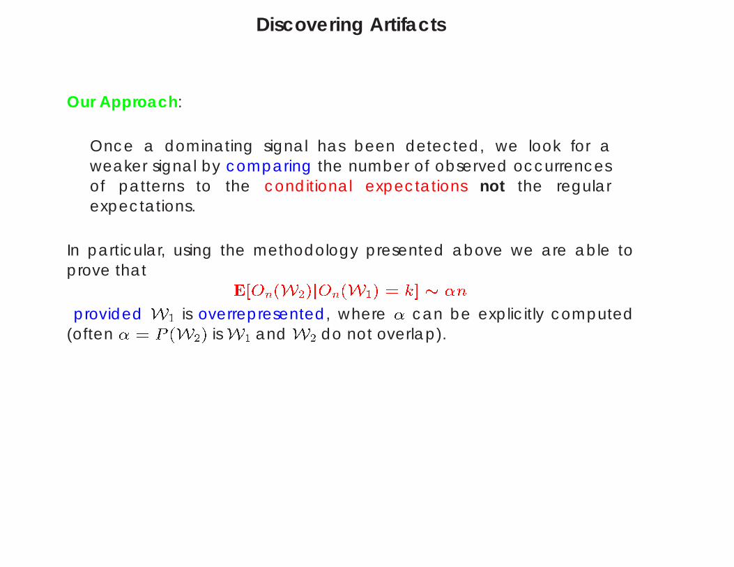
Our Approach:

Once a dominating signal has been detected, we look for aweaker signal by comparing the number of observed occurrencesof patterns to the conditional expectations not the regularexpectations.

In particular, using the methodology presented above we are able toprove that

E[On(W2)jOn(W1) = k] n

provided W1 is overrepresented, where can be explicitly computed(often = P (W2) is W1 and W2 do not overlap).

Polyadenylation Signals in Human Genes

Beaudoing et al. (2000) studied several variants of the well known AAUAAApolyadenylation signal in mRNA of humans genes. To avoid artifactsBeaudoing et al cancelled all sequences where the overrepresentedhexamer was found.

Using our approach Denise and Regnier (2002) discovered/eliminatedall artifacts and found new signals in a much simpler and reliable way.

Hexamer Obs. Rk Exp. Z-sc. Rk Cd.Exp. Cd.Z-sc. RkAAUAAA 3456 1 363.16 167.03 1 1AAAUAA 1721 2 363.16 71.25 2 1678.53 1.04 1300AUAAAA 1530 3 363.16 61.23 3 1311.03 6.05 404

UUUUUU 1105 4 416.36 33.75 8 373.30 37.87 2

AUAAAU 1043 5 373.23 34.67 6 1529.15 12.43 4078

AAAAUA 1019 6 363.16 34.41 7 848.76 5.84 420UAAAAU 1017 7 373.23 33.32 9 780.18 8.48 211AUUAAA 1013 l 373.23 33.12 10 385.85 31.93 3AUAAAG 972 9 184.27 58.03 4 593.90 15.51 34UAAUAA 922 10 373.23 28.41 13 1233.24 –8.86 4034

UAAAAA 922 11 363.16 29.32 12 922.67 9.79 155

UUAAAA 863 12 373.23 25.35 15 374.81 25.21 4CAAUAA 847 13 185.59 48.55 5 613.24 9.44 167AAAAAA 841 14 353.37 25.94 14 496.38 15.47 36

UAAAUA 805 15 373.23 22.35 21 1143.73 –10.02 4068

Application – Information Security

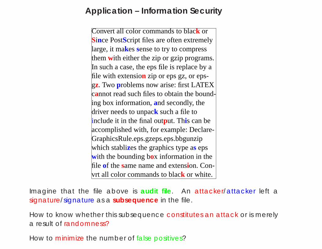
Convert all color commands to black orSince PostScript files are often extremelylarge, it makessense to try to compressthemwith either the zip or gzip programs.In such a case, the eps file is replace by afile with extension zip or eps gz, or eps-gz. Two problems now arise: first LATEXcannot read such files to obtain the bound-ing box information,and secondly, thedriver needs to unpack such a file toinclude it in the final output. This can beaccomplished with, for example: Declare-GraphicsRule.eps.gzeps.eps.bbgunzipwhich stablizes the graphics type as epswith the bounding box information in thefile of thesame name and extension. Con-vrt all color commands to black or white.

Imagine that the file above is audit file. An attacker/attacker left asignature/signature as a subsequence in the file.

How to know whether this subsequence constitutes an attack or is merelya result of randomness?

How to minimize the number of false positives?

Subsequence Matching (Hidden Words)

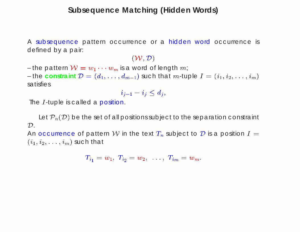
A subsequence pattern occurrence or a hidden word occurrence isdefined by a pair:

(W;D)

– the patternW = w1 wm is a word of length m;– the constraint D = (d1; : : : ; dm1) such that m-tuple I = (i1; i2; : : : ; im)

satisfies

ij+1 ij dj;

The I-tuple is called a position.

LetPn(D) be the set of all positions subject to the separation constraint

D.An occurrence of pattern W in the text Tn subject to D is a position I =

(i1; i2; : : : ; im) such that

Ti1 = w1; Ti2 = w2; : : : ; Tim = wm:

Basic Equation

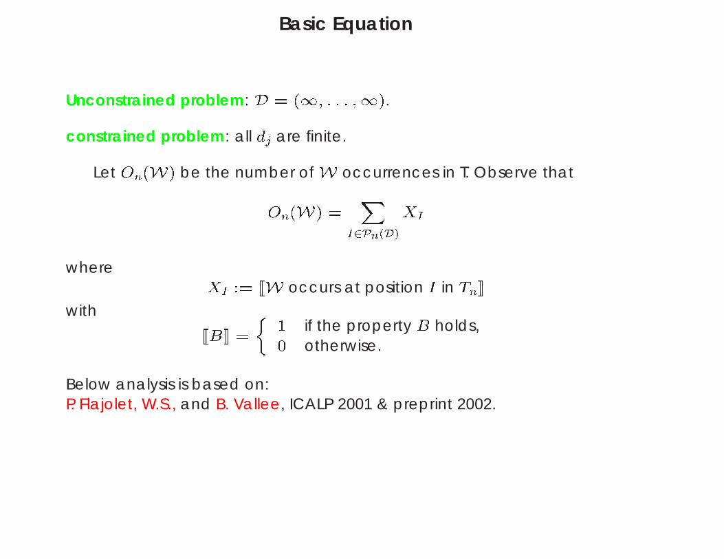
Unconstrained problem: D = (1; : : : ;1).

constrained problem: all dj are finite.

Let On(W) be the number of W occurrences in T. Observe that

On(W) =

XI2Pn(D)XI

where

XI := [[W occurs at position I in Tn]]

with

[[B]] =

1 if the property B holds,

0 otherwise.

Below analysis is based on:P. Flajolet, W.S., and B. Vallee, ICALP 2001 & preprint 2002.

Very Little Theory – Constrained Problem

Let us analyze the constrained subsequence problem. We reduce it to thegeneralized string matching problem using the de Bruijn automaton.

1. The (W;D) constrained subsequence problem will be viewed as thegeneralized string matching problem by assuming that W is the set of allpossible patterns.Example: If (W;D) = a#2b, then

W = fab; aab; abbg:

2. de Bruijn Automaton.Let M = maxflength(W)g 1 (e.g., M = 2 in the above example).Define

B = AM :

De Bruijn automaton is built over B.

De Bruijn Automaton and Analysis

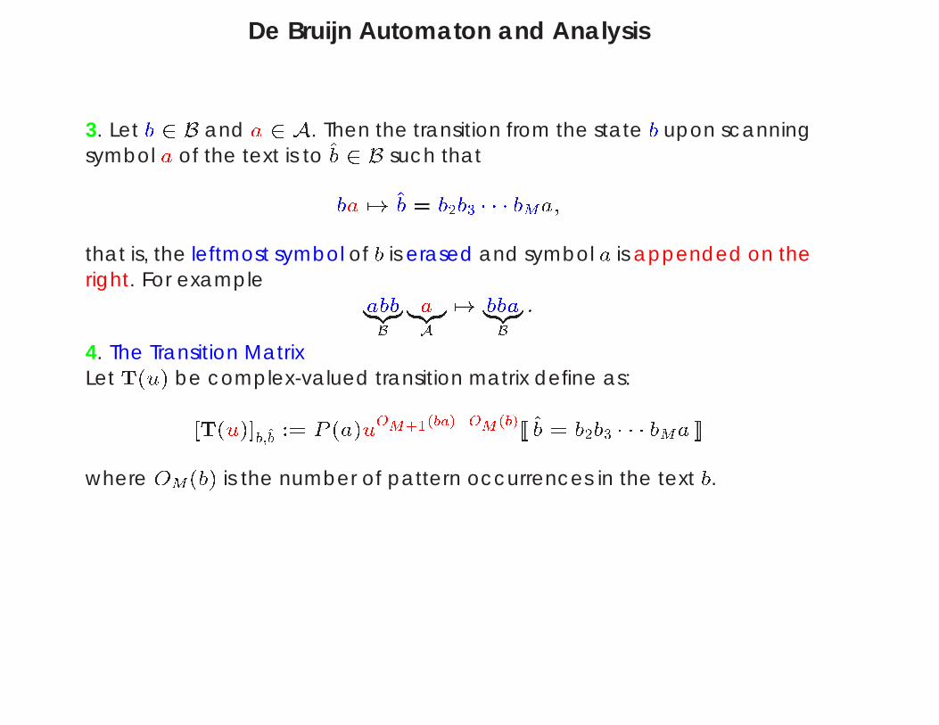
3. Let b 2 B and a 2 A. Then the transition from the state b upon scanningsymbol a of the text is to ^b 2 B such that

ba 7! ^b = b2b3 bMa;

that is, the leftmost symbol of b is erased and symbol a is appended on theright. For example

abb|zB

a|zA

7! bba|zB

:

4. The Transition MatrixLet T(u) be complex-valued transition matrix define as:

[T(u)]b;^b := P (a)uOM+1(ba)OM (b)[[ ^b = b2b3 bMa ]]

where OM(b) is the number of pattern occurrences in the text b.

Example

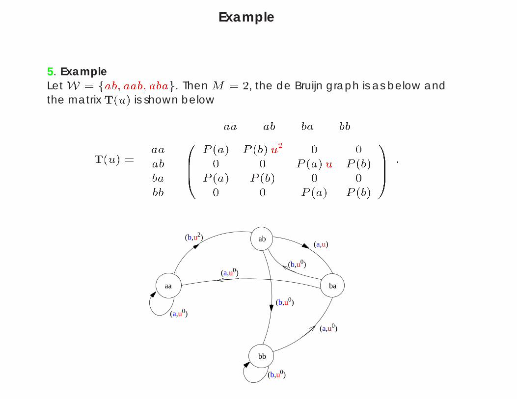
5. ExampleLet W = fab; aab; abag. Then M = 2, the de Bruijn graph is as below andthe matrix T(u) is shown below

T(u) =

aa ab ba bb

aaab

babb

0BB@P (a) P (b)u2 0 0

0 0 P (a) u P (b)

P (a) P (b) 0 0

0 0 P (a) P (b)1

CCA:

ab

aa

bb

ba

(b,u2)

(b,u0)

(a,u)

(a,u0)

(b,u0)

(a,u0)

(b,u0)

(a,u0)

Generating Functions

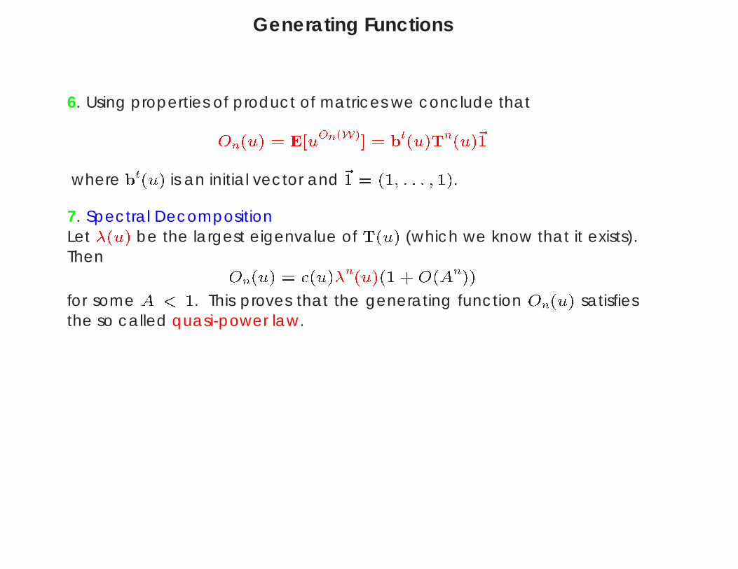
6. Using properties of product of matrices we conclude that

On(u) = E[uOn(W)] = bt(u)Tn(u)~1

where bt(u) is an initial vector and ~1 = (1; : : : ; 1).

7. Spectral DecompositionLet (u) be the largest eigenvalue of T(u) (which we know that it exists).Then

On(u) = c(u)n(u)(1 +O(An))

for some A < 1. This proves that the generating function On(u) satisfiesthe so called quasi-power law.

Final Results

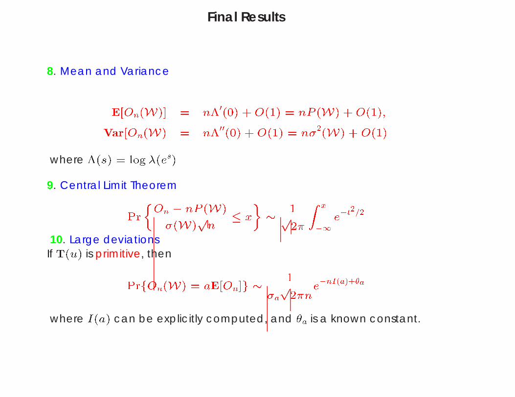
8. Mean and Variance

E[On(W)] = n0(0) +O(1) = nP (W) +O(1);

Var[On(W) = n00(0) +O(1) = n2(W) +O(1)

where (s) = log (es)

9. Central Limit Theorem

PrOn nP (W)

(W)p

n

x

1p2

Z x1

et2=2

10. Large deviationsIf T(u) is primitive, then

PrfOn(W) = aE[On]g

1

ap

2nenI(a)+a

where I(a) can be explicitly computed, and a is a known constant.

Reliable Threshold for Intrusion Detection

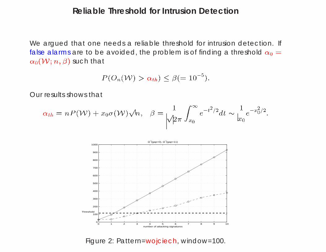
We argued that one needs a reliable threshold for intrusion detection. Iffalse alarms are to be avoided, the problem is of finding a threshold 0 =

0(W;n; ) such that

P (On(W) > th) (= 105):

Our results shows that

th = nP (W) + x0(W)p

n; =

1p2

Z 1x0

et2=2dt 1

x0ex20=2:

0 1 2 3 4 5 6 7 8 9 100

100

200

300

400

500

600

700

800

900

1000

number of attacking signatures

Ω∃(gap=0), Ω∃(gap=11)

Threshold

Figure 2: Pattern=wojciech, window=100.

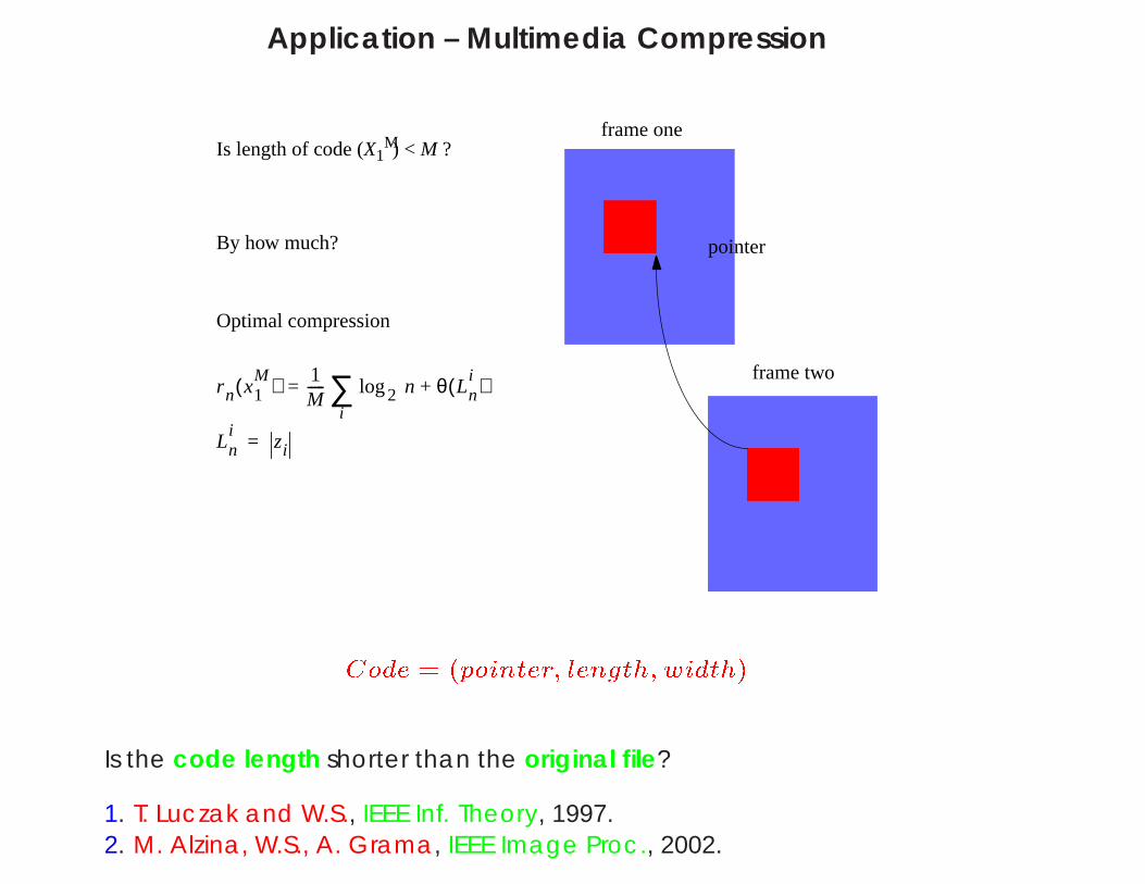
Application – Multimedia Compression

frame one

frame two

pointer

Is length of code (X1M) < M ?

By how much?

Optimal compression

rn x1M( ) 1

M----- log2 n θ Ln

i( )+i

∑=

Lni

zi=

Code = (pointer; length; width)

Is the code length shorter than the original file?

1. T. Luczak and W.S., IEEE Inf. Theory, 1997.2. M. Alzina, W.S., A. Grama, IEEE Image Proc., 2002.

Lossy Lempel-Ziv Scheme

z1 z2 z3( ( (

)

) ) )

z3

z2z1 z3

z2z1

)(

( ))

(

(

source sequenceX1M

of length M

fixed data baseX1n

of lengthn

decoder sequence

X1M

X1M or

)(

(

)

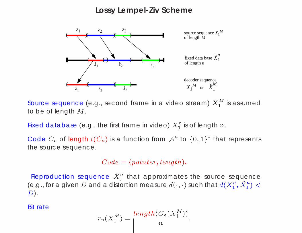
Source sequence (e.g., second frame in a video stream) XM1 is assumed

to be of length M .

Fixed database (e.g., the first frame in video) Xn1 is of length n.

Code Cn of length l(Cn) is a function from An to f0; 1g that representsthe source sequence.

Code = (pointer; length):Reproduction sequence ^Xn

1 that approximates the source sequence(e.g., for a givenD and a distortion measure d(; ) such that d(Xn

1 ;^Xn

1 ) <

D).

Bit rate

rn(XM

1 ) =

length(Cn(XM

1 ))

n

:

Some Definitions

Lossy Lempel-Ziv algorithm partitions according to n the sourcesequence XM

1 into variable phrases Z1; : : : ; Zjnj of length L1n; : : : ; Ljnj

n .

Code length: Since Code=(ptr, length) the length of the code for thesource sequence XM

1 is

ln(XM

1 ) =jnjX

i=1log n+(logLi

n)

and hence the bit rate is

rn(XM

1 ) =

1M

jnjXi=1log n+(logLin):

How much do we gain?

How much do we compress?

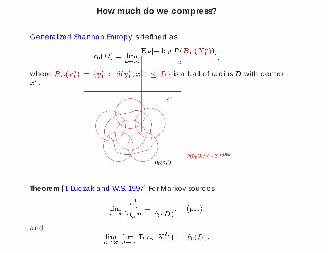
Generalized Shannon Entropy is defined as

^r0(D) = limn!1

EP [ logP (BD(Xn

1 ))]

n

;

where BD(xn

1) = fyn1 : d(yn1 ; xn

1) Dg is a ball of radius D with center

xn1 .

An

BD(X1n)

P(BD(X1n)) ~ 2-r0(D)⋅n

Theorem [T. Luczak and W.S, 1997] For Markov sources

limn!1

L1n

log n=

1^r0(D); (pr:):

and

limn!1

limM!1

E[rn(XM

1 )] = ^r0(D):

Data Structures and Algorithms

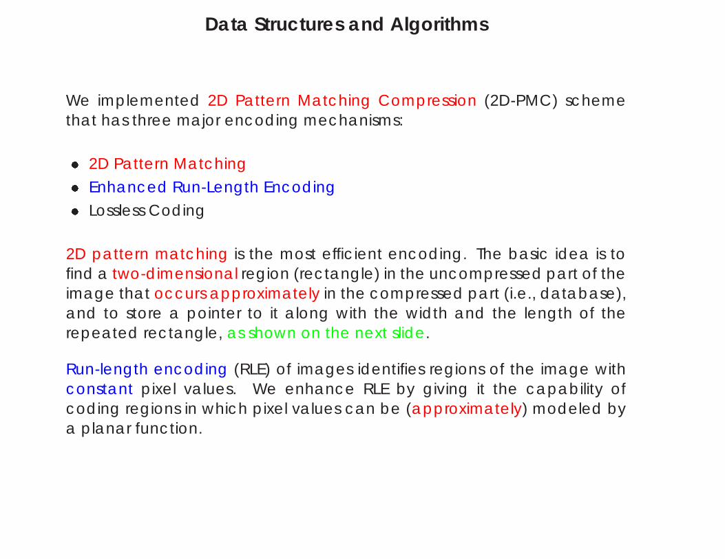
We implemented 2D Pattern Matching Compression (2D-PMC) schemethat has three major encoding mechanisms:

2D Pattern Matching

Enhanced Run-Length Encoding

Lossless Coding

2D pattern matching is the most efficient encoding. The basic idea is tofind a two-dimensional region (rectangle) in the uncompressed part of theimage that occurs approximately in the compressed part (i.e., database),and to store a pointer to it along with the width and the length of therepeated rectangle, as shown on the next slide.

Run-length encoding (RLE) of images identifies regions of the image withconstant pixel values. We enhance RLE by giving it the capability ofcoding regions in which pixel values can be (approximately) modeled bya planar function.

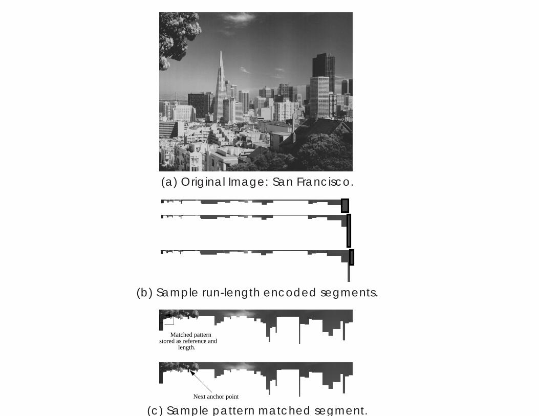
(a) Original Image: San Francisco.

(b) Sample run-length encoded segments.

Matched patternstored as reference and

length.

Next anchor point

(c) Sample pattern matched segment.

Templates

Anchor point

65 18

65 18

105

63 105

65 18

65 18

65 18

105 63

63 105

65 18

63

102 103 65 65 20 219 220 219

17 19 220 221

100 63 65 221

65 65

103 65 65 18

65 65

103

63

65 18

64

65

63

65 18

105

65 18

64

65

63

65 18

64

65

105Template 1: (100, 63, 65, 63, 105, 65)

Template 2: (100, 63, 63, 105, 65, 18)

To identify candidate seed points, we consider a template of k pixelsaround the anchor point.

For example, assume that this template is a 3 2 region with theanchor point as the top-left pixel in the template. The resulting templatecorresponds to a 6-dimensional vector. Figure above illustrates the vectorsfor two templates of dimension 2 3 and 3 2. The problem of findingcandidate seed points then becomes one of finding all vectors in a 6-Dspace that match these vectors at the anchor point in an approximatesense.In the example above, this corresponds to finding all approximateinstances of vectors [100; 63; 65; 63; 105; 65] and [100; 63; 63; 105; 65; 18]

and flagging them as candidate seed points for pattern matches.

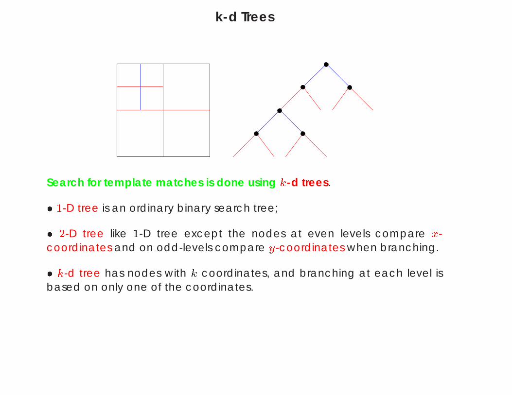
k-d Trees

Search for template matches is done using k-d trees.

1-D tree is an ordinary binary search tree;

2-D tree like 1-D tree except the nodes at even levels compare x-coordinates and on odd-levels compare y-coordinates when branching.

k-d tree has nodes with k coordinates, and branching at each level isbased on only one of the coordinates.

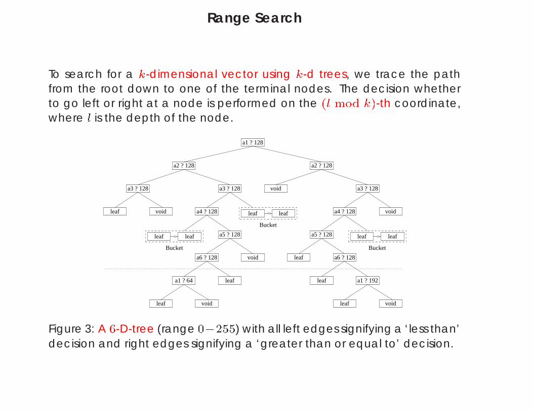
Range Search

To search for a k-dimensional vector using k-d trees, we trace the pathfrom the root down to one of the terminal nodes. The decision whetherto go left or right at a node is performed on the (l mod k)-th coordinate,where l is the depth of the node.

a1 ? 128

a2 ? 128 a2 ? 128

a3 ? 128 a3 ? 128 void a3 ? 128

leaf void a4 ? 128 leaf leaf a4 ? 128 void

Bucket

leaf leaf a5 ? 128 a5 ? 128 leaf leaf

Bucket

a6 ? 128leaf

Bucket

a1 ? 64 leaf

leaf void leaf void

a1 ? 192leaf

a6 ? 128 void

Figure 3: A 6-D-tree (range 0255) with all left edges signifying a ‘less than’decision and right edges signifying a ‘greater than or equal to’ decision.

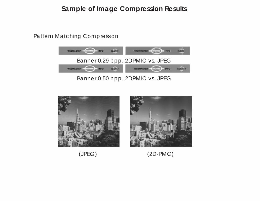
Sample of Image Compression Results

Pattern Matching Compression

Banner 0.29 bpp, 2DPMIC vs. JPEG

Banner 0.50 bpp, 2DPMIC vs. JPEG

(JPEG) (2D-PMC)

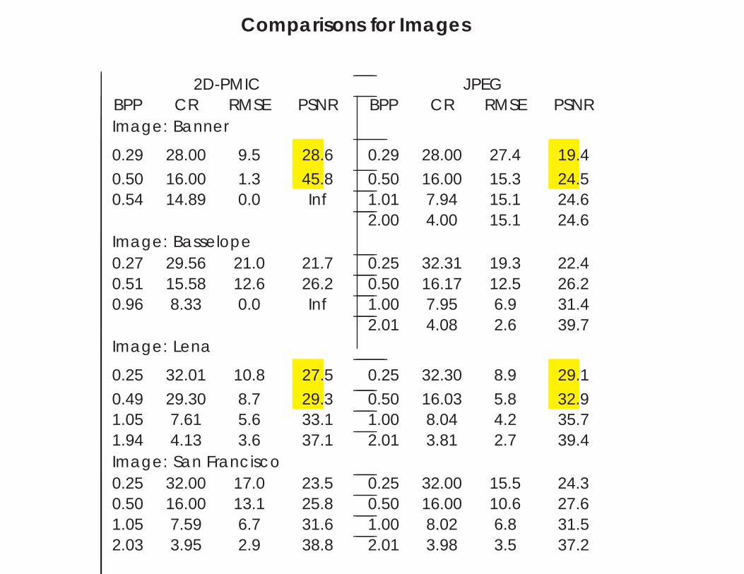
Comparisons for Images

2D-PMIC JPEGBPP CR RMSE PSNR BPP CR RMSE PSNRImage: Banner

0.29 28.00 9.5 28.6 0.29 28.00 27.4 19.4

0.50 16.00 1.3 45.8 0.50 16.00 15.3 24.50.54 14.89 0.0 Inf 1.01 7.94 15.1 24.6

2.00 4.00 15.1 24.6Image: Basselope0.27 29.56 21.0 21.7 0.25 32.31 19.3 22.40.51 15.58 12.6 26.2 0.50 16.17 12.5 26.20.96 8.33 0.0 Inf 1.00 7.95 6.9 31.4

2.01 4.08 2.6 39.7Image: Lena

0.25 32.01 10.8 27.5 0.25 32.30 8.9 29.1

0.49 29.30 8.7 29.3 0.50 16.03 5.8 32.91.05 7.61 5.6 33.1 1.00 8.04 4.2 35.71.94 4.13 3.6 37.1 2.01 3.81 2.7 39.4Image: San Francisco0.25 32.00 17.0 23.5 0.25 32.00 15.5 24.30.50 16.00 13.1 25.8 0.50 16.00 10.6 27.61.05 7.59 6.7 31.6 1.00 8.02 6.8 31.52.03 3.95 2.9 38.8 2.01 3.98 3.5 37.2

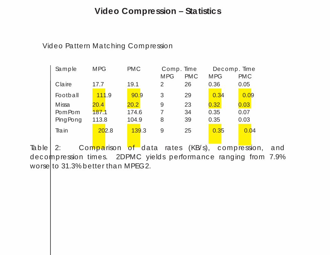
Video Compression – Statistics

Video Pattern Matching Compression

Sample MPG PMC Comp. Time Decomp. TimeMPG PMC MPG PMC

Claire 17.7 19.1 2 26 0.36 0.05

Football 111.9 90.9 3 29 0.34 0.09

Missa 20.4 20.2 9 23 0.32 0.03PomPom 187.1 174.6 7 34 0.35 0.07PingPong 113.8 104.9 8 39 0.35 0.03

Train 202.8 139.3 9 25 0.35 0.04

Table 2: Comparison of data rates (KB/s), compression, anddecompression times. 2DPMC yields performance ranging from 7.9%worse to 31.3% better than MPEG2.