Embed Size (px)
Citation preview

HAL Id: tel-01255290https://tel.archives-ouvertes.fr/tel-01255290
Submitted on 13 Jan 2016
HAL is a multi-disciplinary open accessarchive for the deposit and dissemination of sci-entific research documents, whether they are pub-lished or not. The documents may come fromteaching and research institutions in France orabroad, or from public or private research centers.
L’archive ouverte pluridisciplinaire HAL, estdestinée au dépôt et à la diffusion de documentsscientifiques de niveau recherche, publiés ou non,émanant des établissements d’enseignement et derecherche français ou étrangers, des laboratoirespublics ou privés.
Biomass gasification under high solar heat fluxVictor Pozzobon
To cite this version:Victor Pozzobon. Biomass gasification under high solar heat flux. Thermics [physics.class-ph]. Ecoledes Mines d’Albi-Carmaux, 2015. English. �NNT : 2015EMAC0004�. �tel-01255290�
et discipline ou spécialité
Jury :
le
École Nationale Supérieure des Mines d'Albi-Carmaux conjointement avec l'INP Toulouse
Victor POZZOBON
17 novembre 2015
Biomass gasification under high solar heat flux
ED MEGEP : Génie des procédés et de l'Environnement
Centre RAPSODEE, CNRS UMR 5302, cole des Mines d'Albi-Carmaux
Michel QUINTARD - Directeur de Recherche CNRS - Institut de Mécanique des Fluides deToulouse - Président du jury
Jean-François THOVERT - Directeur de Recherche CNRS - Institut Pprime - RapporteurLaurent VAN DE STEENE - Chargé de Recherche - Laboratoire CIRAD - Rapporteur
Gilles FLAMANT - Directeur de Recherche CNRS - Laboratoire PROMES - ExaminateurFabrice PATISSON - Professeur - cole des Mines de Nancy - Examinateur
Sylvain SALVADOR - Professeur - cole des Mines d'Albi-Carmaux - Directeur de thèseJean-Jacques BEZIAN - Ingénieur - cole des Mines d'Albi-Carmaux - Directeur de thèse
Sylvain SALVADOR et Jean-Jacques BEZIAN


Biomass gasification under high solar heat flux
Victor POZZOBON
Under the direction of
Sylvain SALVADOR and Jean-Jacques BEZIAN
PhD thesis defended on the 17th of November 2015
This work was funded by the French "Investments for the future" program managed by the
National Agency for Research under contract ANR-10-LABX-22-01.
——————————
École Nationale Supérieure des Mines d’Albi-Carmaux


To my father,the man who passed
his appreciation of personal effort andlove of work well done on to me.
A mon père,l’homme qui m’a transmis
son goût de l’effort etson amour du travail bien fait.


Abstract / Résumé
Biomass gasification under high solar heat flux
Abstract:
Concentrated solar energy is as an alternative energy source to power thethermochemical conversion of biomass into energy or materials with highadded value. Production of syngas from lignocellulosic biomass is an example,
as well as the production of carbonaceous residues with controlled properties.This work focuses on the study of the behaviour of a thermally thick beech wood
sample under high solar heat flux (higher than 1000 kW/m2). Two approaches havebeen undertaken at the same time: an experimental study and the development of anumerical model.
Experiments have highlighted a specific behaviour of beech wood under high solarheat flux. Indeed, a char crater, symmetrical to the incident heat flux distribution,forms in the sample. This study has also shown that biomass initial moisture contenthas a strong impact on its behaviour. The dry sample can achieve an energeticconversion efficiency of 90 %, capturing up to 72 % of the incident solar power inchemical form. While, high initial moisture content samples produce more hydrogen,at the price of an energetic conversion efficiency around 59 %. Furthermore, tarthermal cracking and steam reforming are enabled by the temperatures reached(higher than 1200 °C) and the presence of water. Finally, wood fiber orientation hasbeen shown to have only a minor impact on its behaviour.
At the same time, a modelling of the coupled reactions, heat and mass transfersat stake during solar gasification was undertaken. The development of this modelhas highlighted the necessity to implement innovative strategies to take into accountradiation penetration into the medium as well as its deformation by gasification.Numerical model predictions are in good agreement with experimental observations.Based on the model predicted behaviour, further understanding of biomass behaviourunder high solar heat flux was derived. In addition, sensitivity analyses revealed thatArrhenius type models are not fitted for precise intra-particular water behaviourdescription and that the choice of the pyrolysis scheme is key to properly modelbiomass behaviour under high solar heat flux.
Keywords: Solar energy, Pyrolysis, Gasification, High heat flux, Drying, Wood.
v

vi
Gazéification de biomasse sous haute densité de flux solaire
Résumé :
L’énergie solaire concentrée est une source d’énergie alternative pour la conver-sion thermochimique de biomasse en vecteurs énergétiques ou en matériaux àhaute valeur ajoutée. La production d’un gaz de synthèse à partir de biomasse
lignocellulosique en est un exemple, de même que la production de résidus carbonésà propriétés contrôlées.
Ces travaux portent sur l’étude du comportement d’un échantillon de hêtre ther-miquement épais sous de hautes densités de flux solaire (supérieures à 1000 kW/m2).Deux approches ont été développées en parallèles : une étude expérimentale et ledéveloppement d’un modèle numérique.
Les expériences ont permis de mettre en lumière le comportement particulier duhêtre sous de hautes densités de flux solaire. En effet, un cratère de char, dont laforme correspond à celle de la distribution du flux incident, se forme dans l’échantillon.Cette étude a aussi montré que la teneur en eau initiale de la biomasse a un fort impactsur son comportement. Les échantillons secs peuvent atteindre un rendement deconversion énergétique de 90 %, capturant jusqu’à 72 % de l’énergie solaire incidentesous forme chimique. Quant aux échantillons humides, ils produisent nettement plusd’hydrogène, au prix d’un rendement de conversion énergétique aux alentours de59 %. De plus, le craquage thermique et le reformage des goudrons produits par lapyrolyse sont rendus possibles par les températures atteintes (supérieures à 1200 °C)et la présence d’eau. Enfin, il a été montré que l’orientation des fibres du bois n’aqu’un impact mineur sur son comportement.
En parallèle, une modélisation des transferts couplés chaleur matière et desréactions chimiques mis en jeu lors de la gazéification solaire d’un échantillon a étédéveloppée. La construction du modèle a mis en avant la nécessité de recourir à desstratégies innovantes pour prendre en compte la pénétration du rayonnement dansla matière ainsi que la déformation du milieu par la gazéification. Les prédictionsdu modèle montrent un bon accord avec les observations expérimentales. Elles ontainsi permis de mieux comprendre les couplages mis en jeu lors de la dégradation debiomasse sous haute densité de flux solaire. De plus, des analyses de sensibilités ontrévélé que les modèles de type Arrhenius ne permettent pas de décrire finement lecomportement de l’eau à l’intérieur de l’échantillon et que le choix du modèle depyrolyse était capital pour décrire correctement le comportement la biomasse soushaute densité de flux solaire.
Mots-clés : Energie solaire, Pyrolyse, Gazéification, Haute densité de flux,Séchage, Bois.
Table of contents
Abstract / Résumé v
Table of contents ix
Nomenclature xi
Introduction 1
1 State of the art 7Introduction . . . . . . . . . . . . . . . . . . . . . . . . . . . . . . . . . . . 81.1 Solar energy and wood . . . . . . . . . . . . . . . . . . . . . . . . . . 8
1.1.1 Solar energy: electricity and heat . . . . . . . . . . . . . . . . 81.1.2 Wood: a complex material . . . . . . . . . . . . . . . . . . . . 9
1.2 Biomass thermochemical conversion . . . . . . . . . . . . . . . . . . . 111.2.1 Wood drying . . . . . . . . . . . . . . . . . . . . . . . . . . . 111.2.2 Pyrolysis . . . . . . . . . . . . . . . . . . . . . . . . . . . . . . 121.2.3 Gasification of char . . . . . . . . . . . . . . . . . . . . . . . . 141.2.4 Tar cracking and steam reforming . . . . . . . . . . . . . . . . 15
1.3 Solar reactors for biomass gasification . . . . . . . . . . . . . . . . . . 151.4 Modelling . . . . . . . . . . . . . . . . . . . . . . . . . . . . . . . . . 17
1.4.1 Drying . . . . . . . . . . . . . . . . . . . . . . . . . . . . . . . 171.4.2 Pyrolysis . . . . . . . . . . . . . . . . . . . . . . . . . . . . . . 181.4.3 Gasification of char . . . . . . . . . . . . . . . . . . . . . . . . 19
Conclusion . . . . . . . . . . . . . . . . . . . . . . . . . . . . . . . . . . . . 21
2 Materials and methods 23Introduction . . . . . . . . . . . . . . . . . . . . . . . . . . . . . . . . . . . 242.1 Objectives . . . . . . . . . . . . . . . . . . . . . . . . . . . . . . . . . 242.2 Samples . . . . . . . . . . . . . . . . . . . . . . . . . . . . . . . . . . 25
2.2.1 Samples design . . . . . . . . . . . . . . . . . . . . . . . . . . 262.2.2 Samples properties . . . . . . . . . . . . . . . . . . . . . . . . 27
2.3 Experimental apparatus . . . . . . . . . . . . . . . . . . . . . . . . . 292.3.1 Reaction chamber . . . . . . . . . . . . . . . . . . . . . . . . . 292.3.2 The radiation source: an artificial sun . . . . . . . . . . . . . . 36
vii

viii Table of contents
2.4 Artificial sun calibration . . . . . . . . . . . . . . . . . . . . . . . . . 382.4.1 Experimental setup . . . . . . . . . . . . . . . . . . . . . . . . 382.4.2 Experimental procedure . . . . . . . . . . . . . . . . . . . . . 402.4.3 Experimental precautions . . . . . . . . . . . . . . . . . . . . 402.4.4 Screen heating up direct model . . . . . . . . . . . . . . . . . 412.4.5 Screen heating up inverse model . . . . . . . . . . . . . . . . . 422.4.6 Calibration method validation . . . . . . . . . . . . . . . . . . 442.4.7 Results . . . . . . . . . . . . . . . . . . . . . . . . . . . . . . . 472.4.8 Comments on the calibration method . . . . . . . . . . . . . . 48
2.5 Experimental procedures . . . . . . . . . . . . . . . . . . . . . . . . . 482.6 Data processing . . . . . . . . . . . . . . . . . . . . . . . . . . . . . . 50
2.6.1 Gas, tar, water and char final yields . . . . . . . . . . . . . . . 502.6.2 Mass and energy balances . . . . . . . . . . . . . . . . . . . . 51
Conclusion . . . . . . . . . . . . . . . . . . . . . . . . . . . . . . . . . . . . 53
3 Experimental results 55Introduction . . . . . . . . . . . . . . . . . . . . . . . . . . . . . . . . . . . 563.1 Reference case processing . . . . . . . . . . . . . . . . . . . . . . . . . 56
3.1.1 Experimental observations . . . . . . . . . . . . . . . . . . . . 563.1.2 Char properties . . . . . . . . . . . . . . . . . . . . . . . . . . 61
3.2 Crater formation . . . . . . . . . . . . . . . . . . . . . . . . . . . . . 643.3 Impact of fiber orientation . . . . . . . . . . . . . . . . . . . . . . . . 663.4 Impact of initial moisture content . . . . . . . . . . . . . . . . . . . . 683.5 Energy balance . . . . . . . . . . . . . . . . . . . . . . . . . . . . . . 71Conclusion . . . . . . . . . . . . . . . . . . . . . . . . . . . . . . . . . . . . 73
4 Numerical model 75Introduction . . . . . . . . . . . . . . . . . . . . . . . . . . . . . . . . . . . 764.1 Objectives . . . . . . . . . . . . . . . . . . . . . . . . . . . . . . . . . 774.2 Phenomena at stake . . . . . . . . . . . . . . . . . . . . . . . . . . . 774.3 Dimensionless numbers and assumptions . . . . . . . . . . . . . . . . 78
4.3.1 Dimensionless numbers . . . . . . . . . . . . . . . . . . . . . . 784.3.2 Assumptions . . . . . . . . . . . . . . . . . . . . . . . . . . . . 80
4.4 Numerical model . . . . . . . . . . . . . . . . . . . . . . . . . . . . . 824.4.1 Computational domain . . . . . . . . . . . . . . . . . . . . . . 824.4.2 Governing equations . . . . . . . . . . . . . . . . . . . . . . . 834.4.3 Drying model . . . . . . . . . . . . . . . . . . . . . . . . . . . 864.4.4 Biomass degradation scheme . . . . . . . . . . . . . . . . . . . 86
4.5 Physical properties . . . . . . . . . . . . . . . . . . . . . . . . . . . . 884.5.1 Solid phases . . . . . . . . . . . . . . . . . . . . . . . . . . . . 894.5.2 Gas phase . . . . . . . . . . . . . . . . . . . . . . . . . . . . . 91
4.6 Moving mesh strategy . . . . . . . . . . . . . . . . . . . . . . . . . . 914.7 Radiation penetration strategies . . . . . . . . . . . . . . . . . . . . . 95
4.7.1 Near surface penetration . . . . . . . . . . . . . . . . . . . . . 954.7.2 In depth penetration . . . . . . . . . . . . . . . . . . . . . . . 95
4.8 Numerical methods . . . . . . . . . . . . . . . . . . . . . . . . . . . . 98Conclusion . . . . . . . . . . . . . . . . . . . . . . . . . . . . . . . . . . . . 99

Table of contents ix
5 Numerical results 101Introduction . . . . . . . . . . . . . . . . . . . . . . . . . . . . . . . . . . . 1025.1 Assumptions validation . . . . . . . . . . . . . . . . . . . . . . . . . . 1025.2 Comparison with experimental observations . . . . . . . . . . . . . . 1035.3 General behaviour . . . . . . . . . . . . . . . . . . . . . . . . . . . . 105
5.3.1 Drying . . . . . . . . . . . . . . . . . . . . . . . . . . . . . . . 1065.3.2 Tar production . . . . . . . . . . . . . . . . . . . . . . . . . . 1075.3.3 Char steam gasification . . . . . . . . . . . . . . . . . . . . . . 109
5.4 Sensitivity analyses . . . . . . . . . . . . . . . . . . . . . . . . . . . . 1105.4.1 Sensitivity to the drying model . . . . . . . . . . . . . . . . . 1105.4.2 Sensitivity to b fitting parameter . . . . . . . . . . . . . . . . 1135.4.3 Sensitivity to the pyrolysis model . . . . . . . . . . . . . . . . 114
Conclusion . . . . . . . . . . . . . . . . . . . . . . . . . . . . . . . . . . . . 115
Conclusion 117
Appendices 121A Tar analysis . . . . . . . . . . . . . . . . . . . . . . . . . . . . . . . . 123B Wood, char and ash physical properties . . . . . . . . . . . . . . . . . 129C Gaseous species and liquid water physical properties . . . . . . . . . . 133D Radiation near surface penetration model . . . . . . . . . . . . . . . . 137E French extended abstract / Résumé long . . . . . . . . . . . . . . . . 141
Bibliography 155
List of figures 173
List of tables 176

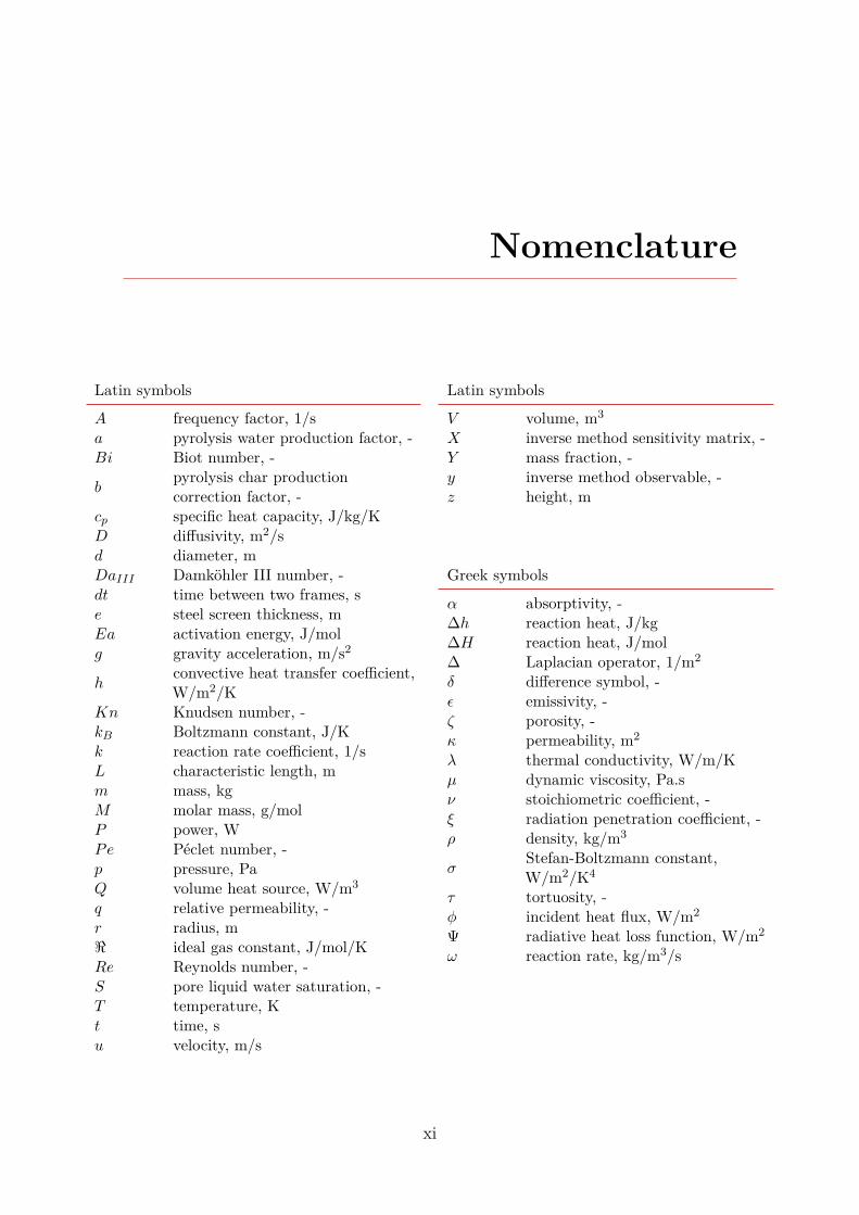
Nomenclature
Latin symbols
A frequency factor, 1/sa pyrolysis water production factor, -Bi Biot number, -
bpyrolysis char productioncorrection factor, -
cp specific heat capacity, J/kg/KD diffusivity, m2/sd diameter, mDaIII Damköhler III number, -dt time between two frames, se steel screen thickness, mEa activation energy, J/molg gravity acceleration, m/s2
hconvective heat transfer coefficient,W/m2/K
Kn Knudsen number, -kB Boltzmann constant, J/Kk reaction rate coefficient, 1/sL characteristic length, mm mass, kgM molar mass, g/molP power, WPe Péclet number, -p pressure, PaQ volume heat source, W/m3
q relative permeability, -r radius, mℜ ideal gas constant, J/mol/KRe Reynolds number, -S pore liquid water saturation, -T temperature, Kt time, su velocity, m/s
Latin symbols
V volume, m3
X inverse method sensitivity matrix, -Y mass fraction, -y inverse method observable, -z height, m
Greek symbols
α absorptivity, -∆h reaction heat, J/kg∆H reaction heat, J/mol∆ Laplacian operator, 1/m2
δ difference symbol, -ǫ emissivity, -ζ porosity, -κ permeability, m2
λ thermal conductivity, W/m/Kµ dynamic viscosity, Pa.sν stoichiometric coefficient, -ξ radiation penetration coefficient, -ρ density, kg/m3
σStefan-Boltzmann constant,W/m2/K4
τ tortuosity, -φ incident heat flux, W/m2
Ψ radiative heat loss function, W/m2
ω reaction rate, kg/m3/s
xi

xii Nomenclature
Subscripts
benzene benzenebw bound watercap capillarychamber reaction chamberchar charcond with tar condenserD Darcyeff effectivefin finalfs focal spotg gas phasegas light gasgasi gasificationI gaseous species indexi frame pixel index in x directionini initial
intrinsicintrinsic
is intermediate solidJ solid species indexj frame pixel index in y directionK reaction indexlim limitlong longitudinalloss losslw liquid watermass massmax maximumno cond without tar condenser
olsestimated using ordinary leastsquare
p paintingpen penetrationpore porepyro pyrolysisrad radiativereac reactions solid phasesand sandsat saturationsp samplest steelsteam steamsur surroundingtar tarth thermalwater waterwood wood
Superscripts
k frame time indexM total number of solid specien total number of frameN total number of gaseous specieO total number of reactionT matrix transposition operatorˆ ordinary least square estimator
Other symbols
. scalar product× matrix productA vector and matrix notationI unit tensorH homothetic center, -n normal vector, -U uniform density law∇ nabla operator, 1/m∏
product∑
sum< > mean‖ ‖ normlim limit

Introduction
Introduction
World primary energy consumption has dramatically grown over the lastthirty years, from 7.14 Gtoe (Giga ton of oil equivalent) in 1980 to13.2 Gtoe in 2012 (Fig. 1). This increase heavily rested upon fossil fuels
(oil, coal and natural gas) and led to the emission of important quantities of greenhouse effect gases in the atmosphere [1]. In turn, these gases induced global warmingand climate change [2]. If not stopped, climate change will lead to more frequentextreme meteorological events. Furthermore global warming will induce a decrease inagricultural yields in tropical and temperate regions, thus endangering food security.It is therefore mandatory to keep, in the coming century, global warming below 2 ◦Cabove pre-industrial temperatures in order to avoid its most dire consequences.
At the same time, a major increase in primary energy consumption is foreseen.In its central scenario, the International Energy Agency predicts a 37 % growth inglobal energy demand by 2040 [3]. While the US Energy Information Administrationprojects a 56 % increase over the same period [4]. This rise will be driven by aincreasing energy consumption in Asia, Africa, the Middle East and Latin America,which will put the world on a path consistent with a 3.6 ◦C global warming. Mankindshould therefore reduce its reliance on fossil fuels and switch to renewable carbonneutral energy sources such as wind, hydraulic, solar power or biomass.
Among these sources, solar energy is believed to be a promising candidatebecause of its versatility and growth potential. Indeed, solar power can directlyproduce electricity thanks to photovoltaic panels. It can also generate low tohigh temperature heat and therefore be used in many domestics and industrialapplications, ranging from producing sanitary water to cracking water moleculesto produce hydrogen [5]. Nevertheless, solar energy is in essence an intermittentenergy source and its storage still remains a challenge to be faced in the years to come.
Biomass is also of interest. This name groups renewable carbonaceous feedstockranging from algae to municipal wastes. Biomass can undergo various transforma-tions in order to be valorized, for instance, as heat via combustion, as methanevia methanation or as syngas via gasification. Syngas is a mixture of hydrogen
1

2 Introduction
1980
1990
2000
2010
2020
2030
2040
0
5
10
15
Year
Worldprimary
energyconsumption(G
toe)
Figure 1: World primary energy consumption. Continuous lines: history, dashed lines: projections.Black: OECD, gray: non-OECD [4]
and carbon monoxide which has a wide number of applications. These applicationsinclude solid oxide fuel cell, gas turbine combustion, running engines, firing in bricksfactory or glass kiln, Fisher Tropsch synthesis, sorted from high to low H2/CO ratio[6]. Gasification is highly endothermic and requires temperatures higher than 800 ◦Cto be led. Classically, the required heat is supplied by burning a fraction of the inletbiomass feed. Two main drawbacks come with this technique: the efficiency withrespect to the biomass is lowered and the produced syngas is diluted by nitrogenfrom the combustion air.
The combination of biomass and solar energy may yield several benefits. Indeed,a synergy of these two energy sources can be envisioned. It is possible to useconcentrated solar energy to power biomass gasification. The produced syngas couldtherefore be considered as a new vector of solar energy. It would also allow to avoidthe biomass combustion associated drawbacks.
After the first oil crisis, studies on the combination of biomass gasification andconcentrated solar power have been undertaken [7]. Yet, the appeal of this fieldof science deflated with the decrease of the the oil barrel price [8]. Nowadays, theinterest in the combination of biomass and solar energy is rising again. Economicalassessments have shown the potential viability of this approach [9], while techni-cal studies have aimed at increasing the efficiency of solar gasification reactors [10, 11].
However, these studies mainly focused on reactor scale experiments and modeling,in fixed bed [7, 12–14], fluidized bed [15, 16] and cyclonic reactors [17–19]. Yet, theydo not permit understanding of biomass and solar power interaction in a scientificvision.

3
The combination of solar energy and biomass still raises several questions atthe sample scale. Radiative power has long been seen only as a way to achievehigh heating rates [20–24] in laboratory scale experiments. It is only recently thatsolar pyrolysis has been studied in order to assess produced char properties [25].The study featured agglomerated wood powder pellets that were suitable to lead athermally thin experiment, but not to understand the interaction between biomassand solar energy. Furthermore, the behaviour of a virgin piece of biomass under highsolar heat flux has never been studied.
In addition to the general behaviour of biomass in itself, the combination ofbiomass and concentrated solar energy raises several questions. For instance, underhigh solar heat flux, biomass would experience high heating rates and high finaltemperature. High heating rates could lead to:
• a very quick vaporisation of the water inside the sample, leading to a sharpincrease of the internal pressure, which may, in turn, induce mechanical failure.This kind of phenomena would depend on sample heating rate, wood structureand initial moisture content
• fast pyrolysis yielding very small amounts of residual carbon solid and therapid surface ablation of the medium
High temperature could enable:
• in situ tar thermal thermal cracking and steam reforming, as well as chargasification
• char thermal annealing
• carbon sublimation, if reached temperatures are high enough
This work aims at tackling these questions. First, literature was reviewed. Ona very practical level, this review of literature has oriented toward to use beechwood (Fagus sylvatica) as model biomass, because it is commonly used whichhas two considerable advantages: allowing for comparison with other studies andincreasing the availability of thermo-physical properties mandatory for numericalmodelling. Then, biomass behaviour under high solar heat flux was investigatedvia an experimental approach as well as a numerical one. On one hand, a newexperimental device allowing the exposure of a thermally thick beech wood sam-ple to heat flux higher than 1000 kW/m2 was built and calibrated. Then, theimpact of wood initial moisture content and wood fiber orientation relative tothe incident heat flux was explored. On the other hand, a new numerical modelwas developed. It features momentum, heat and mass conservation equationsas well as radiation penetration inside of the reacting medium. The agreementbetween experimental observations and numerical predictions is good enoughfor us to be confident in the numerical model descriptive capacities. It was thenused to derive a better understanding of biomass behaviour under high solar heat flux.

4 Introduction
First of all, experimental investigations have highlighted an unreported behaviourof biomass under high solar heat flux. Indeed, a char crater appears at the center ofthe sample. Its shape corresponds to the heat flux distribution at the focal spot of theconcentrating device. Wood initial moisture content is shown to be a key parameterthat has a major impact on every aspect of biomass degradation under high solarheat flux. Surprisingly, wood fiber orientation relative to the incident heat flux isshown to have almost no influence on biomass behaviour. Numerical investigationsyielded valuable insight on the phenomena at stake during solar gasification. Forinstance, they confirm that achieved temperatures lead to tar thermal cracking andthat radiation penetration inside of the sample has to be taken into account.
Manuscript structure
This manuscript is divided into five chapters presenting the work accomplishedduring this PhD. For the sake of readability, it was chosen to keep this manuscriptas short as possible.
Chapter 1 presents a review of the literature dealing with biomass pyrolysis andgasification. As this topic is very wide, a focus was set on solar energy and biomasspyro-gasification combination. The first part briefly presents the main subjects atstake in this work: solar energy and wood. The second part of this chapter highlightsthe mechanisms of biomass thermochemical degradation, from drying to gasification.In the third part, this chapter presents a review of the existing reactors used forbiomass solar gasification. The last part of this chapter brings to light the existingmodel for biomass pyrolysis and gasification.
Chapter 2 deals with the experimental apparatus and data processing methods.It is broken into three thematics. The first one aims at describing extensivelythe new experimental device that was designed during this work. The secondone focuses on a new method of flux mapping at the focal spot of a solar con-centrating device that was developed in order to calibrate the new experimentalapparatus. The last one deals with experimental procedure as well as data processing.
Chapter 3 describes the results obtained thanks to the experimental device. Itreports an unseen behaviour of beech wood under high solar heat flux. Then, itdescribes the effect of two key parameters on biomass solar gasification: wood fiberorientation relative to the incident heat flux and wood initial moisture content.Finally, mass and energy balance closures are reported.
Chapter 4 deals with the numerical model of biomass pyro-gasification thatwas developed during this PhD. This chapter can be divided into three mainparts. The first one presents the phenomena at stake and the assumptions thatwere made in order to model these phenomena. The second part reports theactual equations used to build the model. The last part explains special strate-gies that had to be used to describe the interaction between biomass and solar energy.

5
Chapter 5 presents the results produced by the numerical model. First, thevalidity of the assumptions made is verified and model predictions are comparedto experimental observations. Then, the general behaviour of biomass under highsolar heat flux is commented on. Further insights into the phenomena at stake arederived from the model predictions. Finally, the robustness of the choices made forthe construction of the model are assessed through sensitivity analyses.


CHAPTER 1State of the art
Introduction . . . . . . . . . . . . . . . . . . . . . . . . . . . . . . 8
1.1 Solar energy and wood . . . . . . . . . . . . . . . . . . . . 8
1.1.1 Solar energy: electricity and heat . . . . . . . . . . . . . . 8
1.1.2 Wood: a complex material . . . . . . . . . . . . . . . . . . 9
1.2 Biomass thermochemical conversion . . . . . . . . . . . . 11
1.2.1 Wood drying . . . . . . . . . . . . . . . . . . . . . . . . . 11
1.2.2 Pyrolysis . . . . . . . . . . . . . . . . . . . . . . . . . . . 12
1.2.3 Gasification of char . . . . . . . . . . . . . . . . . . . . . . 14
1.2.4 Tar cracking and steam reforming . . . . . . . . . . . . . 15
1.3 Solar reactors for biomass gasification . . . . . . . . . . . 15
1.4 Modelling . . . . . . . . . . . . . . . . . . . . . . . . . . . . 17
1.4.1 Drying . . . . . . . . . . . . . . . . . . . . . . . . . . . . . 17
1.4.2 Pyrolysis . . . . . . . . . . . . . . . . . . . . . . . . . . . 18
1.4.3 Gasification of char . . . . . . . . . . . . . . . . . . . . . . 19
Conclusion . . . . . . . . . . . . . . . . . . . . . . . . . . . . . . . 21
7

8 Chapter 1. State of the art
Introduction
This chapter aims at providing the required background for understanding thefollowing work. It does not claim to be an extensive review of literature. Theexplored fields, i.e. solar energy and biomass conversion, are extremely wide.
It would therefore be utopian to hope to review them here.
The first part introduces solar energy in terms of technology and potential. Then,it focuses on wood: its composition and properties. The concepts developed here willremain on the general level. The only aim is to familiarize the uninformed readerwith knowledge of solar energy and wood.
The second part describes wood transformation with temperature. Indeed, our ap-plication temperature ranges from 20 °C to more than 1200 °C. Over this range, woodevolution can be broken down into three main steps: drying, pyrolysis and gasification.
The third part presents the past works in the field of biomass solar pyrolysis andgasification. Most of the studies focusing on biomass solar gasification were led atthe reactor scale. It will be an opportunity to present the most conventional solarreactor designs. Studies at the sample scale are also reported. Yet, they remain scarce.
The last part of this chapter focuses on the modelling of the previously describedphenomena. It presents the main description approaches that can be found inliterature. When diverse approaches are available, the advantages and drawbacks ofeach are weighted.
1.1 Solar energy and wood
1.1.1 Solar energy: electricity and heat
The applications of solar can be divided into two main categories: producingelectricity and producing heat. Among the challenges mankind faces in order to usethis energy, storage is of note. Indeed, the incident solar power is intermittent. Itvaries from hour to hour because of the weather. It varies on a daily basis becauseof the day over night cycle. It also varies throughout the year and is not distributeduniformly on the planet.
There are two ways to convert sunlight into electricity. The first way is the useof photovoltaic panels. Photovoltaic panels use the ability of semiconductor, siliconmost of the time, to absorb photons of specific wavelength and convert them intoelectrons. These panel produce direct-current electricity. Depending on its utilization,this electricity can be kept as it is or be transformed into alternative-current, to besent on the grid, for instance. Photovoltaic installation size ranges from a few panelson a rooftop, producing a few kilowatts to large scale utility systems producingseveral megawatts. This versatility leads to a wide potential for installation in sunny

1.1. Solar energy and wood 9
regions [26]. Photovoltaic electricity can be stored using hydroelectric energy storageor battery, yet progress remains to be done in this field of science.
The second way to produce electricity using solar energy is much more clas-sical. Using a solar concentrating device, mirrors and/or lenses, solar beams areconcentrated to produce intense heat. Industrially, heat flux above 1000 kW/m2
(1000 suns) can be achieved. This heat is used to warm up a fluid, for instance steam.It is then recovered from the fluid and turned into electricity via a thermal energyconversion process, e.g. channelling it through a turbine in the case of steam. Thislast part is common with many other power plant technology. Concentrated SolarPower (CSP) plants usually are of large scale and feature storage tanks that allowto store the heated up fluids. This kind of storage allow CSP plants to face solarenergy irregularity and enable them to produce electricity during the late afternoonand evening hours [27].
Process heat is the major consumer of the energy sector [26]. This heat can bedivided into three categories depending on its temperature level:
• low temperature heat, below 100 °C. It is mainly used by the food, the textileand the chemical industries, for activities such as cleaning and drying. Itrepresented 30 % of the heat used in Europe in 2005-2006
• medium temperature heat, above 100 °C and below 400 °C. The main usersare still the food, the textile and the chemical industries. The activities arealso similar as the one using low temperature heat: drying, cleaning, cooking.It accounted for 27 % of the heat used in Europe in 2005-2006
• high temperature heat, above 400 °C. It is used in a wide variety of industriesworking with high temperature processes; examples will be detailed below. Itaccounted for remaining 43 % of the heat used in Europe in 2005-2006
High temperature solar heat is of interest from an industrial point of view becauseis can easily reach fossil fuel firing temperatures without their drawbacks. Indeed,solar energy is clean in the sense that it does not add combustion residues to theprocess. This is why it is used to power pottery firing kilns. This heat can alsobe used to lead high temperature or highly endothermic processes that have animportant carbon footprint, for instance the calcination reaction for lime production[28–31]. Finally, high temperature enable to break the water molecule into hydrogenand oxygen [5]. This could produce the hydrogen required by the rising number offuel cell vehicles [26].
1.1.2 Wood: a complex material
Wood is a complex material that can be considered at several scales. At the molecularlevel, wood is mainly composed of three polymers: cellulose, hemicelluloses andlignin. In addition to them, water, mineral materials (also referred as ash) and lowmolecular weight organic species (referred as extraneous materials) can be found inthe wood. The composition of wood in terms of cellulose, hemicelluloses and lignin

10 Chapter 1. State of the art
plays a major role in determining its properties [32].
Woods are classified into two board categories: hardwoods and softwoods. Thedifferences between these two categories lies at the cellular scale (Fig. 1.1). Hard-woods contain wood cells with open ends. These cells stack on top of one another,forming a channel called a vessel. The vessels serve for sap transportation in thetree. Softwoods do not produce this type of cells, they therefore have no vessels. Insoftwoods, sap transportation is ensured by another type of channel, the tracheids,which are also present in hardwoods. Softwoods are therefore less porous thanhardwoods.
(a) Hardwoods (b) Softwoods
Figure 1.1: Hardwoods and softwoods anatomy [33]
At the macroscopic scale, wood can be considered as an homogeneous porousmedia with anisotropic physical properties. Indeed, transport properties of wooddepend on the direction. It is easy to understand when considering that its structureis made of long parallel tubes. Three directions have to be considered: longitudinal(parallel to the fiber, the tree growth direction), radial (from the heart of the trunktoward the bark), orthoradial (perpendicular to longitudinal and radial). For a givenwood structure, heat and mass transfers are favoured in the longitudinal direction.For instance, the longitudinal permeability is as much as five thousand times higherthan the radial permeability [34]. Most of the time, radial and orthoradial propertiescan be assumed to be equal.

1.2. Biomass thermochemical conversion 11
1.2 Biomass thermochemical conversion
With an increase in temperature wood undergoes several transformations (Fig. 1.2).The first one is drying, which takes place around 100 °C. Then comes torrefaction,close to 250 °C, which can be seen as the very beginning of pyrolysis. Even thoughthis field of science receives more and more attention, it will not be consideredin this review. From 400 °C to 800 °C, wood undergoes pyrolysis. During thistransformation, it will turn into three main products: light gases, tar and char.Above 800 °C, char can be oxidized by steam and/or carbon dioxide to producesyngas. This step is referred as gasification. For further reading on biomass thermaldegradation, one can refer to the pioneering work on Grønli [35].
Figure 1.2: The different steps of biomass degradation
1.2.1 Wood drying
Water can be found in wood under three forms: gaseous (water vapour), free liquidand bounded to the solid matrix (mainly to cellulose). At room temperature, watercan move out of the wood porous matrix by diffusion. Around 100 °C, it is drivenout by a pressure gradient induced by the boiling of liquid water. The distributionof water between these three forms is governed by a liquid-vapour equilibrium.Drying is the first major transformation undergone by the wood. This endothermictransformation is very complex. For the sake of simplicity, only drying near 100 °Cwill be considered. This type of drying is often referred as high temperature drying.
Consider a wood sample homogeneous in temperature. At 100 °C, and ambientpressure, liquid water inside of wood starts boiling. The pressure increases locally

12 Chapter 1. State of the art
and drives the steam out of the sample. Thus, water leaves the wood. Once all ofthe liquid water has been vaporised, bounded water starts separating from the woodmatrix and evaporates until none remains. This is, of course, a simplified description.One should keep in mind that liquid and bounded water can move inside of thewood cavities [36]. Depending on the local temperature and pressure steam cancondense. Furthermore, drying has an impact on the wood structure (contraction,distortions, cracks). It can locally lead to mechanical failure hindering the woodrobustness [37–39].
High temperature drying has been shown to have an impact on the subsequentsteps of biomass degradation. It modifies the yields of the pyrolysis step by increasingthe proportions of light gases as well as char, therefore lowering tar production[21, 40]. This trend is consistent with an increase in wood initial moisture content:the more water, the more light gases and char are produced. Finally, the presenceof water also changes the nature of produced tars. Indeed, the tar produced bypyrolysis after high temperature drying have been reported to be less acidic thanthose produced after a softer drying [40].
1.2.2 Pyrolysis
Pyrolysis takes place from 400 °C to 800 °C. During this transformation, the drybiomass polymers are broken down into a solid carbon residue called char and morethan 300 different molecules [41]. These molecules can be sorted into two categories.Light gases (or simply gas) appellation covers the light hydrocarbons that remainsgaseous at ambient temperature, usually from H2 to C3H8. Tar encompass theremaining molecules that are gaseous at pyrolysis temperature, but liquid at roomtemperature. The proportions and compositions of these three products can varydepending on the pyrolysis conditions, for instance reported char yields range from7 to 50 % [42, 43]. The three main factors influencing pyrolysis products distributionare: the pyrolysis final temperature and heating rate and biomass initial composition[41, 44–50]. The main trends are (Fig. 1.3):
• a high initial lignin content in wood leads to an increased char yield, whilehigh cellulose and hemicellulose content lead to more important gas and taryields [51–53]. Thus, hardwoods produce more gas and tar but less char thansoftwoods. Furthermore, minor components may also modify pyrolysis outcome.Alkali salts contained in wood ash tends to catalyse pyrolysis reactions andfavour CO2 production over CO [51, 54].
• the higher the heating rate, the more tar is produced. It is explained by thefact that at high heating rates, the produced tar are quickly expelled from thebiomass. This prevents them from undergoing substantial cracking. However,low heating rate conditions can even allow for a tar to condense [55] whichincreases tar residence time inside of the sample and therefore their probabilityof undergoing cracking and repolymerisation. Liquid tar are called intermediate

1.2. Biomass thermochemical conversion 13
liquid compound [22, 56] or metaplastic phase because of its very high viscosity[57].
• the higher the pyrolysis final temperature, the less tar is produced. Indeed, hightemperatures favour tar decomposition into gas and char. This phenomenon isknown as tar thermal cracking.
Heating rate
Low Medium Fast Flash
Final
temperature
500
◦C
1000
◦C
Figure 1.3: Pyrolysis products distribution [58]. Black: char, gray: tar, white: gas
In addition, it is commonly known that pyrolysis produces water. Yet, onlyfew authors deal with water production during pyrolysis by considering it as anindividual specie [59–63]. Most of the time, water produced by pyrolysis is takeninto account as tar because it condenses at room temperature. It can be estimatedthat between 8 and 37 % of the initial dry biomass turns into water during pyrolysis.
As glimmered, pyrolysis is a complex and wide topic. In addition to the varietyof its operating conditions, reviewing the subject is made even more difficult bythe variety of feedstock (ranging from algae to tire scraps [64, 65]). Neverthe-less, beech wood is the most commonly studied feedstock after coal. For thesake of readability, it was chosen to focus this review on fast pyrolysis of wood(heating rates higher than 100 K/min) and its impact on subsequent char gasification.
The way pyrolysis is led has an impact on gasification. It was shown that charreactivity during gasification varies depending on pyrolysis conditions. High heatingrates tend to produce more reactive chars. These chars internal geometry offers

14 Chapter 1. State of the art
a higher specific surface area [46, 47, 49]. It is explained by the rapid escape ofgas and tar from the sample preventing tar cracking reactions from occurring thusthe deposit of char coming from tar repolymerisation reactions [23]. Their oxygenand hydrogen contents are also higher which indicates that more reaction sites areavailable for gasification [66].
High temperature and high pressure during pyrolysis tend to limit char reactivity.High temperature favours a reorganising of char matrix and pore coalescence.It decreases the number of reaction sites and specific surface area available forgasification [44, 50]. This phenomenon is referred as thermal annealing. Highpressure during pyrolysis yields similar effect on char reactivity [67].
Solar heating allows to achieve high heating rates as well as high final tem-peratures. To this date, only one study has focused on the wood solar pyrolysis[25]. The authors focused on the chemical properties of char obtained by solarpyrolysis of beech wood pellets. They have shown that solar pyrolysis of woodleads to highly reactive char with high specific surface area. They also foundthe limit: final temperature above 1600 °C has an adverse effect on char reac-tivity, which can be explained by thermal annealing. Apart from this study, thebehaviour of a biomass sample in itself under high solar heat flux remains unexplored.
1.2.3 Gasification of char
Gasification is a group of heterogeneous chemical reactions consuming carbonaceousfeedstock. During gasification reactions, an oxidative reagent, most of the time steamand/or carbon dioxide, reacts with char to create hydrogen and carbon monoxide(Eq. 1.1 to 1.3). At the end of this stage, only syngas and ash remain.
Cs + H2O −→ CO + H2, ∆Hreac = −131.1 kJ/mol, water reforming reaction (1.1)
Cs + CO2 −→ 2CO, ∆Hreac = −172.5 kJ/mol, Boudouard reaction (1.2)
Cs + 2H2 −→ CH4, ∆Hreac = +74.4 kJ/mol, one of the methanation reactions (1.3)
CO + H2O ←→ CO2 + H2, ∆Hreac = +41.1 kJ/mol, Water Gas Shift reaction (1.4)
Char-steam and char-carbon dioxide gasification are the ones that have been themost widely studied [7, 12–15, 17, 19, 43, 46, 47, 49, 68–71]. It has been highlightedthat char-steam gasification is kinetically 2 to 5 times faster than char-carbon dioxidegasification. In addition, it yields a hydrogen richer syngas. Studies on the combinedsteam and carbon dioxide gasification have shown an interaction between the tworeagents leading to a reaction rate higher than just the sum on the two individualones [52, 72].
As discussed earlier, char reactivity is influenced by pyrolysis conditions: thehigher the specific surface area, the higher the reaction rate. Minor species play an

1.3. Solar reactors for biomass gasification 15
important role in determining the gasification reaction rate. Alkali salts found in thewood can have a strong catalytic effect on the gasification reactions [47, 69, 70, 73],while silicon has an inhibitory effect [69].
1.2.4 Tar cracking and steam reforming
Tar produced by the pyrolysis of biomass are classified in two ways according to theirmolecular weight and their degree of breakdown. The first classification considerslight, medium and heavy molecular weight tar. The second classifies tar as primary,secondary and tertiary tar depending on the extent of thermal cracking that theyhave undergone. Two broad kinds of tar breakdown reactions exist: thermal crackingand steam reforming. Both of them require temperatures higher than 800 °C to beof considerable importance.
Tar thermal cracking reactions breakdown the main part of medium and heavytar into light tar (light aromatics) and gas. Some tar recombine to form thermallystable heavy tar (PolyAromatic Hydrocarbons or PAH), the refractory tar [74, 75].This phenomenon grows in importance with an increase in temperature: 90 % ofthe tar produced by a pyrolysis at 600 °C have undergone thermal cracking once1200 °C is reached.
Tar steam reforming includes a wide range of chemical reactions which transformtar into carbon monoxide and hydrogen (Eq. 1.5) [76, 77]. These are kineticallyfavoured by high temperatures; with temperature below 800 °C, only light andmedium tar can be reformed, while temperatures above 1200 °C enable the reformingof the majority of the heavy tar.
CxHyOz + (x− z)H2O −→ xCO + (x− z +y
2)H2 (1.5)
1.3 Solar reactors for biomass gasification
Solar pyrolysis and gasification have been led in a wide variety of reactor designs.The aim of these reactors is to offer the best heat transfer of the concentrated solarenergy to the biomass, while controlling the reactive atmosphere. A review of theliterature has recently been proposed [78].
• fluidized bed reactors are of interest because they can achieve a good thermalhomogeneity and high heat exchange rates [23, 79]. Furthermore, ash can beadded to the bed, hence, catalysing gasification reactions. These reactors alsohave drawbacks. Most of the time the steam used as fluidizing agent has to beinjected in excess, hence, lowering the system efficiency. Fluidized bed reactorsrequire a narrow particle size distribution of the input feedstock [12, 43] or theuse of a fluidizing medium, such as sand [80]. Furthermore, this reactor designshows a poor capacity in cracking the tar [56]

16 Chapter 1. State of the art
• fixed bed reactors are well known and robust reactors [7, 12–14, 43, 47, 81].Yet, their use for solar gasification exhibits a very specific problem. Gasificationtakes place on the top of the bed, at the focal spot, leaving only ash. Ash canaccumulate here. Because of ash low absorptivity and thermal conductivity[81–83], it forms a radiative shield on the top of the bed which reduces thequantity of radiation absorbed by the reactor [12, 16, 43]
• vortex reactors expose the feedstock in suspension in a swirling vector gas[17–19, 28, 29]. The main drawback of this setup is the need for a very finelyground feedstock (< 200 µm)
• tubular reactors have also been used to lead a more unconventional type ofchar gasification: gasification in supercritical water [68, 73, 84]. The mainadvantage of this technique is that carbon dioxide dissolves into water, thereforefacilitating the separation of syngas from other products
• rotary kilns reactors have also been used for both solar biomass gasification[56, 72] and limestone solar decarbonatation [30, 31]
Independent of the reactor design, the way in which the feedstock is exposed tothe incident heat flux has an impact on the reactor behaviour. The first way is todirectly expose the feedstock to the incident heat flux: the solar beams enter thereactor through a window and are directly absorbed by the reacting medium. Thesecond way is to use an absorber heated up by the incident heat flux which emitspart of the incident energy towards the inside of the reactor.
Direct heating allows to precisely locate the focal spot inside the reactor(Fig. 1.4 A). At the focal spot, very high heating rates can be achieved around1000 K/s [7, 14, 17, 18, 56, 86]. A window is set through the aperture that theincident heat flux crosses in order to prevent the reagents or the products to freelyescape the reactor and maintain a controlled atmosphere. This window induces adecrease of about 10 % of the maximum incident heat flux [87]. Furthermore, itneeds to be protected from any soiling. Indeed, darking the window would increaseits absorption of the incident power, increasing its temperature and potentiallyleading to its mechanical failure.
Indirect heating relies on an intermediary absorber that mediates the transfer ofconcentrated solar energy to the feedstock (Fig. 1.4 B) [12, 15, 43, 68, 72, 84]. Theabsorber makes uniform the emission inside of the reactor. It can also have a betterspectral absorption than the feedstock, thus increasing solar energy absorption.Nevertheless, it induces heat losses by radiative emission towards the surrounding.
Regarding solar reactor design, it can be noted that the larger the reactor, thegreater its thermal inertia. This is important for solar reactors because it enablesthem to keep working even without sun for a limited period of time [43].

1.4. Modelling 17
(a) A vortex reactor allowing direct heat of the feed-stock [85]
(b) A packed bed reactor equipped with anintermediary absorber [81]
Figure 1.4: Two reactor designs featuring direct and indirect feedstock heating
1.4 Modelling
Modelling each of the aforementioned phenomena is a challenge in itself. For each ofthem, several approaches exist depending on the needs it has to answer. It partlyexplains why there are only few attempts to build models that couple these complexphenomena [21, 88].
1.4.1 Drying
Three broad categories of models can be found in literature. The models of the firstcategory take into account the actual liquid-vapour equilibrium [89]. These modelscan finely predict the transport of steam as well as free and bounded water. Theyare able to properly capture condensation. However, they have two limitations: theirimplementation might be challenging and their computational cost is much higher
18 Chapter 1. State of the art
than that of the other models.
The second kind of models, or Arrhenius type models, describe water vaporisationas a thermally activated phenomenon taking place around 100 °C [88, 90–93]. Thesemodels are used when drying is not the main focus of the study. Most of the timetemperature of the medium will rise far above 100 °C. Hence, the model only aimsat removing water from the medium. Nevertheless, some refinement might be addedto them, by adding the possibility for steam to condense if the temperature is lowenough [94].
The last type of models is referred as thermal models. They consider that dryingtake place at fixed temperature (usually 100 °C). If moisture is still present, allsupply heat will be consumed by drying. Once moisture has been removed, thetemperature is allowed to raise again. This kind of modelling induces sharp dryingfront that may lead to numerical problems [95].
For further detail on the methods used to model wood drying, one can refer tothe discussion in [91].
1.4.2 Pyrolysis
Predicting the outcome of the pyrolysis of any feedstock is a particularly difficulttask. As mentioned before, the parameters of influence are many and the expectedproducts can be considered at different levels: mass dynamic and thermal behaviourof the sample or gaseous products composition.
Most of the models solve a heat and mass transfer problem coupled with biomassdegradation. Some models neglect mass transfer [96] while others use a Darcy lawto describe the gas flow inside of the sample. Authors generally do not discussthe possibility to correct Darcy’s law using Forchheimer equation [97, 98] nor thepossibility to use one or two temperatures approaches [99]. Furthermore, onlyfew authors defend their assumptions. Very few authors use characteristic timesapproach to weigh the relative role of phenomena at stake beforehand [23, 100, 101],even less use dimensionless numbers [23].
Accurately describing biomass degradation into char, tar and gas is key[12, 88, 102, 103]. Indeed, poorly predicting biomass degradation leads to a biasedprediction of the heat consumed by the biomass pyrolysis, having in turn an impacton the temperature field prediction, which controls biomass degradation.
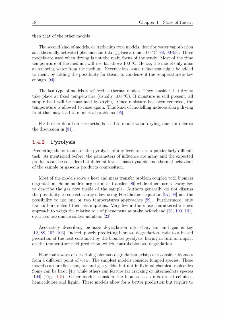
Four main ways of describing biomass degradation exist; each consider biomassfrom a different point of view. The simplest models consider lumped species. Thesemodels can predict char, tar and gas yields, but not individual chemical molecules.Some can be basic [45] while others can feature tar cracking or intermediate species[104] (Fig. 1.5). Other models consider the biomass as a mixture of cellulose,hemicellulose and lignin. These models allow for a better prediction but require to
1.4. Modelling 19
know the different product yields beforehand [105]. The third category are capableof predicting the production of individual species considering 10 to 50 chemicalreactions, the most renowned being Ranzi model [106]. The last ones, referredas FG-DVC (for Functional Group-Depolymerization, Vaporisation, Crosslinking)were first used for coal pyrolysis prediction. They describe biomass cellulose,hemicelluloses and lignin as group monomers linked by chemical bonds. Thesemodels then predict depolymerisation and repolymerisation at the monomers levelbased on temperature and pressure conditions [107].
For all of these models, limitations exist. The main one is that they are validatedagainst given sets of experimental measurements, making them depend on theconditions in which the experiments were conducted. For instance, a degradationscheme may yield very good predictions for slow, low temperature pyrolysis andbe unable to properly predict the products distribution in the case fast, hightemperature pyrolysis. Sadly, few experimental studies have dealt with combinedhigh heating rate and high final temperature conditions [42]. Furthermore, to ourknowledge, no biomass degradation scheme as been established for these particularconditions. This lack of studies might be explained by the adverse effect of highheating rate and high final temperature. It makes this configuration unappealing forboth people who would like to maximise tar production or to enhance char yield.
Besides, biomass geometry changes during pyrolysis. The volume of the charresidue is around 35 % of the volume of the initial sample [108, 109]. This change ingeometry has an impact on heat and mass transfer through the sample, thus, modi-fying the pyrolysis products’ distribution [110, 111]. Nevertheless, this phenomenonis neglected most of the time. It is only recently that some authors have been ableto take it into account using a prescribed deformation method [88].
Gas
Wood Tar
Char
(a) A simple lumpedspecies scheme [45]
Gas Secondary tar
Wood Tar
Intermediate solid Char
(b) A more complex lumped specie scheme [103]
Figure 1.5: Different types of lumped species biomass degradation schemes
1.4.3 Gasification of char
There are two main interests behind modelling gasification reaction: predicting theproducts distribution and predicting the gasification reaction rate.

20 Chapter 1. State of the art
Predicting the distribution of the products of char gasification can been reasonablywell done using the principle of minimum energy of Gibbs free energy [17, 52, 68].This method assumes that the system has reached its thermodynamic equilibrium.It may not always be the case in actual reactors, yet this approach allows to draw ageneral behaviour: a higher temperature favours carbon monoxide and hydrogenover methane. Over 1100 °C, only carbon monoxide and hydrogen remain. Pressurehas an adverse effect on hydrogen production. The higher the pressure, the moremethane is produced.
Predicting char gasification reaction rate is a more challenging task. It can beundertaken at two levels: the particle scale in thermally thin thermogravimetricanalyses or the reactor scale. The first one aims at better understanding thephenomena taking place during gasification, while the second produces kineticparameters readily usable to describe feedstock behaviour inside a reactor.
As stated before, gasification heterogeneous reactions are influenced by oxidativeatmosphere composition, sample specific surface area and mineral content. Thechemistry at stake is quite complex. Proper description requires serial and parallelreactions, reactions between the products themselves, inhibitory effects of theproducts, catalytic effects of minerals and structure evolution [14, 19, 46, 47, 52, 71].
Simplified, macroscopic approaches have also been proposed. They aim atoffering simple kinetic parameters that can be used to describe gasification reactionat the reactor scale [14, 112, 113]. These kinetics only consider the reaction ratedependency on the main oxidative reagent, i.e. steam or carbon dioxide. A review ofthe available kinetics can be found in [46].
Reactor scale modelling allows to compute species distribution in time andspace [13, 15]. Numerous models have been proposed for reactor scale gasification[16, 114]. For more specific modelling of solar gasification reactors, one can refer to[7, 13, 15, 19, 43, 47, 68, 81].
Few authors have undertaken the modelling of the behaviour of a single thermallythick char sample undergoing gasification. Modelling such a phenomenon is chal-lenging because the model has to take into account the deformation of the samplegeometry. Indeed, in this configuration, the external layer of the reacting medium inconsumed first while the core remains unconsumed. This configuration falls intothe shrinking core model category which is known to be challenging to model usingstandard modelling approaches. Most of the proposed model are restricted to 1Dconfigurations.
To this date, in the pyrolysis and gasification field, few models are able to describesuch a phenomenon in 2D or 3D. Three of them are of note. The first one considersthe gasification of a char pellet (agglomerated char particles) taking the fragmentationof the pellet into account [115]. The number of fragments produced by the pellet isprescribed, while their consumption is described using a phase function approach.

1.4. Modelling 21
The second model describes the combustion of a biomass sphere in a grate furnace.The particle is decomposed into four layers that shrink as the biomass undergoescombustion. The last one describes the pyrolysis and ablation of the thermal shieldof a space shuttle during is entry in the atmosphere [116]. Under these conditions,char is not ablated by gasification but by the high shear stress air flow. Nevertheless,the configurations are very similar. In this particular case, the deformation is notprescribed: front tracking method is coupled with Arbitrary Lagrangian Euleriantechnique [117].
Conclusion
This chapter aimed at providing a basic background on solar energy and biomassthermal degradation. The key point of this chapter is that concentrated solar energyallows to produce high heat flux and to reach temperatures above 1200 °C. Exposinga wood sample to such a heat flux leads to its thermal degradation. The three mainsteps of this degradation are: drying, pyrolysis and gasification. These steps arecomplex in essence and influence one another. Only few experimental and numericalworks report an in depth investigation of biomass behaviour under high solar heatflux. This PhD aims at contributing to the reduction of this gap in literature. Afterthis literature review, beech wood (Fagus sylvatica) was chosen as the model biomass.Indeed, this feedstock is commonly used which has two considerable advantages:allowing for comparison with other studies and increasing the availability of thermo-physical properties mandatory for numerical modelling. Given the chosen focus, i.e.thermally thick samples, this work may more easily apply to other technologies suchas packed bed reactors or ablative heat shields.


CHAPTER 2Materials and methods
Introduction . . . . . . . . . . . . . . . . . . . . . . . . . . . . . . 24
2.1 Objectives . . . . . . . . . . . . . . . . . . . . . . . . . . . . 24
2.2 Samples . . . . . . . . . . . . . . . . . . . . . . . . . . . . . 25
2.2.1 Samples design . . . . . . . . . . . . . . . . . . . . . . . . 26
2.2.2 Samples properties . . . . . . . . . . . . . . . . . . . . . . 27
2.3 Experimental apparatus . . . . . . . . . . . . . . . . . . . 29
2.3.1 Reaction chamber . . . . . . . . . . . . . . . . . . . . . . 29
2.3.2 The radiation source: an artificial sun . . . . . . . . . . . 36
2.4 Artificial sun calibration . . . . . . . . . . . . . . . . . . . 38
2.4.1 Experimental setup . . . . . . . . . . . . . . . . . . . . . . 38
2.4.2 Experimental procedure . . . . . . . . . . . . . . . . . . . 40
2.4.3 Experimental precautions . . . . . . . . . . . . . . . . . . 40
2.4.4 Screen heating up direct model . . . . . . . . . . . . . . . 41
2.4.5 Screen heating up inverse model . . . . . . . . . . . . . . 42
2.4.6 Calibration method validation . . . . . . . . . . . . . . . 44
2.4.7 Results . . . . . . . . . . . . . . . . . . . . . . . . . . . . 47
2.4.8 Comments on the calibration method . . . . . . . . . . . 48
2.5 Experimental procedures . . . . . . . . . . . . . . . . . . . 48
2.6 Data processing . . . . . . . . . . . . . . . . . . . . . . . . 50
2.6.1 Gas, tar, water and char final yields . . . . . . . . . . . . 50
2.6.2 Mass and energy balances . . . . . . . . . . . . . . . . . . 51
Conclusion . . . . . . . . . . . . . . . . . . . . . . . . . . . . . . . 53
23

24 Chapter 2. Materials and methods
Introduction
The following chapter describes the experimental device designed and theprocessing methods developed to explore the behaviour of beech wood underhigh solar heat flux. It can be divided into fives parts.
The first part sums up the objectives that were to be met by the experimentaldevice and by the results processing methods. Two goals lie behind these objectives:better understanding of biomass behaviour by direct observation and producingresults that will later be used to confront model predictions.
The second part presents the samples and their design strategy. Samples arethermally thick pieces of beech wood. Two sets of samples with two different fiberorientations relative to the incident heat flux are used in this study. Furthermore,initial moisture content of the samples is a key parameter and will therefore be varied.
The third part describes the experimental device in detail. It is composed of twodifferent pieces: the reaction chamber and the radiative source. Building a devicecapable of exposing biomass to high radiative heat flux is known to be challenging.That is why, along with the description of the device, some problems faced duringthe conception are discussed and solution strategies are presented here.
Part four focuses on a particular problem that was faced during the conceptionof the experimental device: the calibration of the artificial sun. A new heat fluxmeasurement method specific to high radiative heat flux mapping was developed[118]. This method is based on an inexpensive apparatus and basic inverse methods.They are used to compute the heat flux distribution from IR camera recordings.This technique is not specific to the experimental device developed in this work andcould be used to calibrate any solar concentrating system.
The fifth part presents the experimental protocols that were followed for everyrun made.
The last part details the data processing methods that were used to deriveinformation on the biomass behaviour from the measurements. Two processes aredescribed: how pyrolysis yields are obtained from experimental data and how massand energy balances are derived.
2.1 Objectives
The objectives that the experimental device had to meet fall into two categories:primary and secondary objectives. Primary objectives encompass the very basicfeatures that allow for biomass exposure to high radiative heat flux.

2.2. Samples 25
The primary objectives are:
a. Exposing a thermally thick biomass sample to heat flux higher or equal to1000 kW/m2. Even though it seems really basic, this objective might turn outto be challenging. Indeed, reaching heat flux as high 1000 kW/m2 is uncommon
b. Preventing the presence of oxygen in the vicinity of the sample. Given the levelof temperature at stake during pyrolysis and gasification, oxygen would reactwith volatile matters and char. This combustion would bias the observationsand induce safety problems
c. Avoiding the spoilage of the window crossed by the incident heat flux, in orderto prevent its heating and mechanical failure. This constraint is identical tothe one found in direct heating solar reactors
The secondary objectives have a wider scope. They cover additional features thatallow further investigation of biomass behaviour and later confrontation of modelpredictions to experimental observations.
The secondary objectives are:
a. Following the sample mass throughout a run. It should, in principle, allow forthe identification of phenomena by attributing to them a trend in the massloss curve
b. Monitoring temperatures at the sample surface as well as inside the sampleitself. Indeed, reported temperature levels are correlated to the phenomena atstake in the biomass degradation process
c. Computing sample transformation mass yields in terms of drying water, gastar and char
d. Analysing gas composition
e. Analysing tar composition. This should allow to investigate tar thermal history,i.e. whether they have undergone thermal cracking or not
f. Establishing mass and energy balances of the system. Achieving closure wouldindeed be a token of the quality of the experiments
2.2 Samples
The samples were first designed then characterized. The objective lying behind thesample design is to explore as much as possible biomass behaviour under high solarheat flux. As identified before, sample fiber orientation relative to the incident heatflux may be a key parameter, as well as its initial moisture content. Samples weremade out of beech wood only. The influence of wood type was not studied in this work.

26 Chapter 2. Materials and methods
2.2.1 Samples design
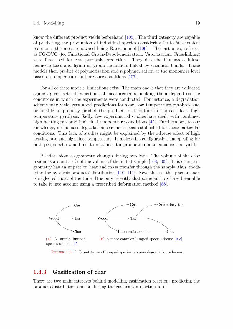
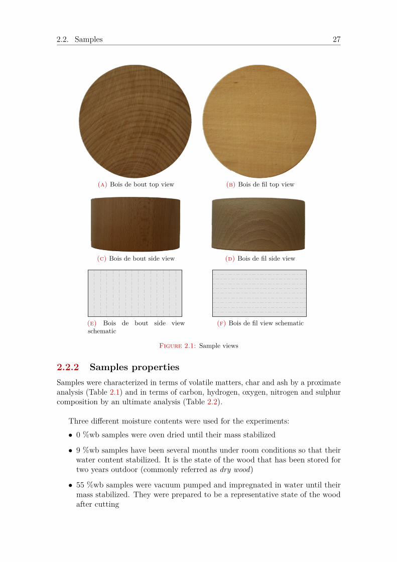
The sample design faces two major constraints: producing thermally thick sampleand allowing to easily model the sample geometry. As the first constraint is obvious,the second is more subtle. Because of the wood anisotropy and the scale of thestudy, i.e. the sample scale, it is important to anticipate how to model the feedstock.Indeed, if the wood fibers are randomly oriented from sample to sample, the futurenumerical model should be able to handle this problem. In order to facilitatemodelling of the sample, it was chosen to first work with wood cylinders whose fibersare parallel to the revolution axis of the cylinder (Fig. 2.1). The top surface ofthe cylinders would be exposed to the incident heat flux. Hence, this configurationwould allow for a 2D axysymmetrical modelling of the sample geometry under theassumption that radial and orthoradial physical properties of the wood are equal.Such samples fall into the special category of wood pieces: bois de bout. Bois de boutare pieces for which a special care is taken so that the wood fibers would be per-pendicular to a desired surface, in our case the top and bottom surfaces of the cylinder.
The sample size was determined using a pre-model1 of biomass thermal degrada-tion. The design criterion was that the lateral and bottom surfaces of the sampletemperature would not exceed 50 °C after a 5 minutes exposure. This designprocedure leads to the choice of 10 cm diameter, 5 cm high samples.
Bois de bout samples represent a very specific configuration; it would be bold tothink that this configuration is representative of the behaviour of biomass under highsolar heat flux whatever the orientation of the wood fibers relative to the incidentheat flux. So, in order to assess this configuration impact, another set of sampleswas prepared: bois de fil samples (Fig. 2.1). Bois de fil samples have their fibersperpendicular to the cylinder revolution axis. They can be seen as the extremeopposite of bois de bout samples in terms of fiber orientation.
For practical reasons, it was not possible to carve bois de bout and bout de filsamples out of the same tree. Tree composition can vary depending on where itgrew or the weather it was exposed to. In order to assess the potential differencesbetween the two used trees, proximate and ultimate analysis (Tables 2.1 and 2.2, seenext section) can be used. The results between the two beech woods are very closeand in good agreement with values reported in literature [119]. The samples cantherefore be considered to be made of the same material.
One should note that the modelling of bois de fil samples is not possible using a2D axisymmetrical geometry. They indeed require to be described using 3D geometry.
1This numerical model describes beech wood drying and pyrolysis. It was implemented underComsol. This model was used during the experimental device design stages for sizing purposes.Yet, because of this software intrinsic limitations, its development was stopped in favour of animplementation of the model using OpenFOAM CFD toolbox.
2.2. Samples 27
(a) Bois de bout top view (b) Bois de fil top view
(c) Bois de bout side view (d) Bois de fil side view
(e) Bois de bout side viewschematic
(f) Bois de fil view schematic
Figure 2.1: Sample views
2.2.2 Samples properties
Samples were characterized in terms of volatile matters, char and ash by a proximateanalysis (Table 2.1) and in terms of carbon, hydrogen, oxygen, nitrogen and sulphurcomposition by an ultimate analysis (Table 2.2).
Three different moisture contents were used for the experiments:
• 0 %wb samples were oven dried until their mass stabilized
• 9 %wb samples have been several months under room conditions so that theirwater content stabilized. It is the state of the wood that has been stored fortwo years outdoor (commonly referred as dry wood)
• 55 %wb samples were vacuum pumped and impregnated in water until theirmass stabilized. They were prepared to be a representative state of the woodafter cutting

28 Chapter 2. Materials and methods
Bois de bout Bois de fil
Volatile matters 15.2 14.2Char 84.3 85.0Ash 0.5 0.8
Table 2.1: Wood proximate analysis (%wt)
Bois de bout Bois de fil
Carbon 48.78 49.96Hydrogen 5.98 5.62Oxygen 43.93 44.10Nitrogen 0.35 0.32Sulphur 0.96 -
Table 2.2: Wood ultimate analysis (%wt)
A change in wood moisture content induces a change in its geometry. Dryinginduces shrinkage, while water impregnation induces swelling. Because of the inducedswelling or shrinkage, the wood density varies with moisture content. By measuringsample mass and volume, it is possible to calculate its apparent density. Table 2.3reports the different wood apparent density and porosity assuming beech wood bulkdensity being 1500 kg/m3 [120, 121]. These measurements were repeated at least 6times in order to derive a standard deviation.
Moisture content Density (kg/m3) Porosity (%)
0 %wb 652 ± 40 57 ± 2.69 %wb 579 ± 38 61 ± 2.655 %wb 535 ± 8.0 65 ± 1.2
Table 2.3: Sample density and porosity versus moisture content
Sample spectral properties are also of importance. Indeed, they govern theamount of radiative energy that is absorbed and emitted by the sample. Beechwood reflectivity was measured for both bois de bout and bois de fil configurations(Fig. 2.2). Furthermore, given the fact that the sample will undergo pyrolysis, after afew seconds the exposed surface will be made of char and not wood. Char reflectivitywas therefore also measured (Fig. 2.2). Finally, the absorptivities of the materialswere computed with respect to the lamp spectrum (see Section 2.3.2). Bois debout and bois de fil have the same absorptivity of 0.37, while char absorptivity is 0.88.

2.3. Experimental apparatus 29
0 2 4 6 8 100
0.2
0.4
0.6
0.8
1
Wavelength (µm)
Reflectivity
Figure 2.2: Beech wood and char reflectivities. Gray lines: beech wood, black line: char
2.3 Experimental apparatus
During a run, the sample is placed in an enclosure referred to as the reaction chamber.The reaction chamber allows to expose the sample to the concentrated solar heatflux. It also ensures that no oxygen is allowed in the vicinity of the sample, monitorssample mass and temperature, captures tar and permits to analyse the gas.
For this study, no solar concentrating system was readily available. Therefore anartificial sun was used instead. This kind of radiative source has long been used toemulate solar energy in terms of density and spectrum. They are now becomingmore and more widespread because they allow to study high temperature phenomena[28, 87, 122, 123] without suffering from the main drawback of solar energy, i.e.intermittence. The applications of this kind of device were recently and extensivelyreviewed in [124]. One should note that these devices are also referred to as imagefurnaces.
The reaction chamber is positioned on a scale (Fig. 2.3). Special care wastaken in ensuring scale stability. It was placed on a massive independent stain-less steel table so that it is not subject to vibrations. Furthermore, the artificialsun is placed above the reaction chamber, yet, no contact point exists between the two.
The reaction chamber is described first, then the radiative heat source is presented.
2.3.1 Reaction chamber
The objectives of the reaction chamber are numerous. The main idea behind thereaction chamber design (Fig. 2.4 and 2.5) is that: placing the sample in a sweptchannel allows to expose the sample through a windowed aperture, evacuate the

30 Chapter 2. Materials and methods
2
1
3
4 5
6
Figure 2.3: Picture of the experimental device. 1: artificial sun, 2: reaction chamber, 3: gassampling device, 4: scale, 5: stainless steel table, 6: temperature recording devices
produced gas and tar, condense the tar just downstream of the sample in a condenserand analyse the remaining gas. The following parts describe how the reactionchamber fulfils these objectives.
2.3.1.1 Controlling the atmosphere and exposing the sample
The atmosphere around the sample can be easily controlled by sweeping it with aninert gas such as nitrogen. Furthermore, purging the reaction chamber with morethan 10 times its volume before a run would ensure that no oxygen remains in thevicinity of the sample.
The reaction chamber has to allow for a continuous exposure of the samplethroughout a 5 minutes run. The main problem is that, while undergoing pyrolysis,the sample produces abruptly gas and tar. Because of wood fiber orientation, these

2.3. Experimental apparatus 31
12
4
6
7
5
3
810
9
11
Figure 2.4: Schematic of the reaction chamber. 1: nitrogen inlet, 2: porous medium, 3: quartzwindow, 4: sample, 5: incident heat flux, 6: thermocouples, 7: static mixer, 8: condenser,9: insulating material, 10: cotton trap, 11: gas sampling probe
12
34
5
67
Figure 2.5: Schematic of the reaction chamber, cut view, without insulating material. 1: nitrogeninlet, 2: porous medium, 3: sample, 4: static mixer, 5: condenser, 6: cotton trap, 7: gas samplingprobe
gases are expelled toward the quartz window. If the tar would come in contact withthe window, they would undergo thermal cracking and leave a carbon layer on thewindow. It would increase the window absorptivity, hence its temperature, andquickly lead to its mechanical failure, allowing oxygen to enter the reaction chamber.
In order to prevent this kind of incident from happening, the nitrogen sweep flowrate has to be high enough to drive gas and tar away from the window. Yet, the flowshould be laminar in order to prevent turbulent mixing. Furthermore, it was alsothought that maximizing sweeping flow shear stress on the sample surface wouldfurther increase its capability to drive away the produced gas and tar (Fig. 2.6).Hence, a porous medium was set on the sweeping flow trajectory upstream to the

32 Chapter 2. Materials and methods
sample, so that a sweeping flow would be in a laminar plug flow configuration uponreaching the sample. In order to save the time and cost of a trial and error approach,this concept was first tested using numerical models: the pyrolysis pre-modelproduced the gas and tar flow rate expelled by the sample. Fluent was used tocalculate the required nitrogen flow rate and the porous media length so that thewindow would stay clean. Numerical design advised a sweeping flow rate of 60 l/min.Experiments showed it could be safely lowered to 40 l/min. Lowering the sweepinggas flow rate comes with advantages: produced gases are less diluted which facilitatesits analysis, reducing the condenser payload (Section 2.3.1.2) and being more costefficient. Therefore, the nitrogen flow rate was set to 40 l/min for all experimentsusing a mass flow meter and a controller.
The porous medium is a packed bed of 2 mm diameter alumina spheres. It hasbeen observed that these spheres absorb water contained in air. Therefore, thisporous medium should be dried before a run in order to prevent its drying frombiasing the mass monitoring.
(a) Poiseuille flow (b) Plug flow
Figure 2.6: Nitrogen sweeping flow configurations
2.3.1.2 Condenser
Once driven away from the sample, the gas, tar and water are forced into a tarand water condensing device referred to as condenser. This condenser aims atcapturing all the tar and water produced by the sample during a run. Hence,the downstream flow would be free of tar and water. It could thus be analysedfor gas composition. Regarding water, one point arises. Water stopped by thecondenser is the sum of water coming from the sample drying as well as thewater produced by the pyrolysis. In this study, water produced by the pyrolysiswill be accounted as tar. Water will refer to the water coming from the sample drying.
The condenser takes advantage of the fact that tar is by definition a liquid atroom temperature. By lowering the flow temperature below 0 °C, tar and watercondense into small droplets. These droplets can then be captured using a cottonfilter. To ensure that tar condenses throughout a run, the condenser temperature hasto remain below 0 °C. This could be achieved in two ways: by continuously cooling

2.3. Experimental apparatus 33
the condenser or by cooling the condenser before the start of a run at a temperaturelow enough so that it would not reach 0 °C before the end of that run. These twomethods have their own drawbacks. The first one implies supplying cool liquid tothe condenser and therefore hanging tubes from the reaction chamber. This mightbe a problem for the continuous weighing of the reaction chamber (Section 2.3.1.4).The second implies that the condenser would be efficient only for a certain amountof time. The second method was thought to be the best. Thus, a transient condenserwas designed for 5 minutes run.
The condenser is removable, so that it can be immersed in cold liquid before a run.Liquid nitrogen was chosen as cooling medium (77 K, or -196 °C). For conveniencesake, the condenser should not be too heavy. Hence, its volumetric heat capacityhas to be high enough so that enough negative calories could be stored for a run.After a search, it was found that aluminium was the best available solution becauseof its high heat capacity, low density, thermal stability and availability. Hence, thecondenser was made out of aluminium.
The main part of the condenser is a porous media made of aluminium spheres.This design was chosen because it enables a good solid gas contact and a low pressuredrop. The main fraction of the negative calories is stored in the aluminium spheres.Upstream of the aluminium spheres packing is a static mixer made of a set ofunevenly perforated plates. Indeed, the sweeping flow being laminar, hot tar, waterand gas do not mix with nitrogen. If sent with no mixing inside of the condenser,this hot core flow would heat up only the central part of the condenser, leaving thelateral parts as thermally dead volume (Fig. 2.7). Downstream of the aluminiumspheres is a cotton trap. This trap is set to capture tar droplets and aerosols escapingthe condenser. Indeed, preliminary runs have shown that the aluminium spheres donot intercept all of the tar droplets. It was therefore mandatory to place a filter tostop them.
Finally, the reaction chamber was surrounded by insulating material in order toprevent water contained in air to condense on the reaction chamber outer surfacenear the condenser.
2.3.1.3 Gas and tar analysis
A continuous gas analysis throughout a run was too complex. It was chosen to resorton batch sampling. Three gas samples were taken at the outlet of the cotton trapover different time laps during a run: t = 0 to 1 minute, 2 to 3 minutes and 4 to 5minutes. Gas were stored in Tedlar bags and then analyzed using a microGC. Thereported species are: H2, CO, CO2, CH4, C2H2, C3H8, C2H6 and C2H4. These speciesare thought to represent more than 95 % of the gas emission [100, 125]. Becauseof the sweeping flow, these species are diluted by nitrogen. Nitrogen represents 90%vol of the analyzed gas feed, which is low enough not to hinder measurements quality.
In addition to providing the gas composition, gas analysis is a way of computing

34 Chapter 2. Materials and methods
(a) Without static mixer
(b) With static mixer
Figure 2.7: Schematic of the flow pattern inside of the condenser
sample gas yield. Indeed, average gas composition can be also used to calculate theaverage gas production rate. As the nitrogen flow rate and the stream compositionare known, it is possible to compute the average gas flow rate and thus sample gasproduction rate.
Cotton containing tar was stored in air tight boxes and sent to CIRAD laboratoryfor tar composition analysis. Tar was desorbed in acetone before being analysed usinggas chromatography coupled with mass spectrometry. Four analyses were performed:tar produced by bois de bout sample for the three initial moisture contents. 9 %wbinitial moisture content samples tar were analysed twice in order to assess the run torun repeatability of the results.
2.3.1.4 Mass and temperature monitoring
During a run, the whole system is weighed using a scale. Therefore, the systemmass loss can be accounted for. A bichromatic radiometer is set in such a waythat it measures sample surface temperature at the focal spot. A set of threethermocouples is placed inside of the sample in order to monitor its core temperature.

2.3. Experimental apparatus 35
A Precisa EP 2220M scale was used to monitor the reaction chamber mass. It hasa range of 2.220 kg and a precision of 1 mg. In order not to perturb the mass signal,special care was taken in using long, loose and flexible cables for thermocouplesconnections and nitrogen feeding. Because the condenser is removable, the scale canbe used to determine different quantities:
• when the condenser is not fitted into the reaction chamber, gas, tar and waterfreely escape the reaction chamber. Under these conditions, the mass signalaccounts for the sample mass loss evolution
• when the condenser is fitted into the reaction chamber, tar and water arestopped. Therefore, only gas escapes the system. The mass signal onlyaccounts for the gas production rate
As a complement to continuous mass monitoring, mass measurements weretaken before and after a run. They allow to calculate wood consumption, water,char, gas and tar average production rates. Before a run, sample mass msample, ini
and reaction chamber mass mchamber, ini were measured. After a run, samplemass msample, fin and reaction chamber mass mchamber, fin were measured again.Exposed samples contain a char residue produced by pyrolysis which was notconsumed by gasification (Fig. 2.8). This char was scratched away from thesample and its mass mchar was taken. Then, the void left by the char was filledwith thin sand in order to measure the volume of the crater in the wood. Themass of this sand msand was taken. Knowing, the sand and the wood density, itis possible using Eq. 2.1 to determine the mass of wood mwood consumed during a run.
mwood = msandρwood
ρsand
(2.1)
Figure 2.8: Schematic cut view of a sample after exposure. Dark gray: moist wood area, lightgray: dry wood area, black: char residue
Sand density was measured every day, right before using it to measure the cratervolume. Indeed, sand is an hygroscopic material and could therefore absorb waterwhich would change its density.
In addition to mass measurements, temperatures were also recorded. Holes weredrilled into the samples and type K and S thermocouples were used to monitortemperatures at several points inside of the samples. The thermocouples were placed2 cm below the exposed surface one on the sample revolution axis and two 1 cmaway from the axis (Fig. 2.4). Surface temperature was also monitored using a
36 Chapter 2. Materials and methods
bichromatic radiometer. Its measurement capacity ranges from 600 to 1800 °C.Finally, a thermocouple was set at the outlet of the reaction chamber, so that outletflow temperature could be monitored.
2.3.2 The radiation source: an artificial sun
Artificial suns are basically made of xenon arc lamp and a concentrating mirror(Fig. 2.9). The lamp is placed at the first focal point of an elliptical mirror. Themirror intercepts the radiation coming from the lamp and redirects it toward itssecond focal point. The system is enclosed in a casing for both safety and technicalreasons. Firstly, because the lamp produces very intense radiations that can damagethe eyes of the people looking at it. Secondly, the whole system dissipates atremendous amount of heat. Half of the lamp electric consumption is directlyconverted to heat and half of the produced radiation (one quarter of the lamp electricconsumption) is intercepted by the casing. Air fans are used to remove this heat.The casing helps to properly direct the air flow around the lamp. Furthermore, ashutter is placed on the casing so that exposure can be controlled without turningon and off the lamp.
In our case, a former cinema lantern was used as casing. Inside of it, a 4 kWelamp xenon arc lamp (OSRAM XBO 4000 W/HS) was used. According to themanufacturer, the efficiency of the conversion to radiation is about 50 %. In order tointercept the maximum amount of radiation, the largest mirror available was used(semi major axis: 430 mm, semi minor axis: 205 mm). It has a 12.98° aperture angle.This aluminium coated mirror was supplied by Edmund Optics (Ref. 90-972).
The spectrum of the radiation coming out of the casing was measured usingOcean Optics USB2000 spectrometer (Fig. 2.10). It can be seen that the incidentradiation spectral distribution is close to the solar spectrum at sea level through oneair mass. Both distributions exhibit a thermal continuum, yet they differ by someabsorption and emission band associated to gases. The spectrum produced by theartificial sun is slightly shifted toward low wavelength and features emission rays ofxenon between 400 and 600 nm. While solar spectrum features absorption rays ofH2O and CO2.
Determining the incident heat flux at the focal spot of the artificial sun is achallenging task. This problem has been approached using various methods. Insome cases a radiometer [127] or equivalent [128] is used to map the focal spot. Thismethod is time consuming and offers a low spatial resolution map. Yet, it yields anabsolute value of the incident heat flux and requires no external scaling factor. Inother cases a CCD camera is used to record a gray value image of a water-cooledtarget [123, 124]. Then using an external measurement, often a radiometer reading,a scaling factor is applied to the recorded image. This method allows for a highresolution but relies entirely on the external scaling factor and the use of a high-endwater-cooled target. One last way of mapping the heat flux distribution is to run

2.3. Experimental apparatus 37
(1)
(2)
(3)
(4)
(5)
(6)
(7)
Figure 2.9: Schematic of the artificial sun. 1: 4 kW xenon arc lamp, 2: elliptical mirror, 3: a ray,4: shutter, 5: casing, 6: air inflow, 7: air outflow
400 600 800 1000 1200 1400 1600 1800 2000
Wavelength (nm)
Figure 2.10: Power spectral distribution (y axis: arbitrary units). Black: solar spectrum at sealevel through 1 air mass [126], gray: incident radiation spectrum
the device at minimal power, for example using the moon instead of the sun for anoutdoor dish [129]. Pictures can be taken and processed to yield high resolutionincident heat flux map. Then, the actual map can be computed using the ratio ofthe two source powers. Sadly, this is not possible for certain devices such as xenonarc lamps because their minimal power is very close to their nominal operatingcondition.
The former methods being out of reach, it was therefore mandatory to develop anew method that would allow to map the incident heat flux distribution at the focal

38 Chapter 2. Materials and methods
spot of solar concentrating systems.
2.4 Artificial sun calibration
The idea behind the method2 that is described in this section is quite simple. Itis thought that by placing a screen on the artificial sun beams trajectory andmonitoring its warming up, it would be possible to determine the incident heat fluxintercepted by the screen.
Heat flux distribution mapping is a widespread problem that can be foundin numerous industrial situations. Among the various methods that have beendeveloped for the determination of the incident heat flux, the inverse methods are ofparticular interest. Inverse methods associate a problem, a mathematical model andexperimental measurements to compute quantities of interest. They adopt a reversepoint of view in comparison to the classical approaches. For example, a classicalheat transfer problem is the determination of a temperature field from knownboundary condition, heat source and material properties. This is called a directproblem. On the contrary, an inverse problem is the determination of boundaryconditions, heat source and/or material properties from temperature measurements.A model linking the measurements to the desired value is built; it is called an inversemodel. This approach has been applied with success to a wide variety of problems,such as the design of insulation protection [130], or the sizing of a heat exchanger [131].
The following sections present: the experimental setup used to collect data, themathematical treatment of the data and the results, i.e. the heat flux distribution.
2.4.1 Experimental setup
To map the incident heat flux, a screen is set in front of the artificial sun (Fig. 2.11).Thus, the beams coming out of it are intercepted by the screen. As beams energyis absorbed by the screen, its temperature rises. The temperature variations arerecorded by a 320x240 IR camera with a working range between 8 and 12 µm. Screenexposure is controlled by a shutter placed on the light trajectory before the focalspot. The focal spot of this device is known to be 32 cm away from the lamp housecasing.
In order to have a flat emissivity of 0.79 in the camera working range, oneside of the screen was painted with a black paint. Temperature was monitoredon the painted side of the screen. Far from the focal spot, the painted side of thescreen was illuminated (Fig. 2.11). At the focal spot, the bare steel side of thescreen was illuminated reducing the absorbed energy by a factor of about 2 (Fig. 2.12).
2 This method was published in Solar Energy journal (DOI: 10.1016/j.solener.2015.04.021 ). Itis reproduced with the editor authorisation.

2.4. Artificial sun calibration 39
(1)
(2)
(3)
(5)
(6)
(4)
y x
z
Figure 2.11: Calibration apparatus schematics, defocused configuration. 1: 4 kWe xenon arclamp, 2: elliptical mirror, 3: a ray, 4: camera, 5: shutter, 6: screen, black line: paint
(1)
(2)
(3)
(4)
(5)
(6)
Figure 2.12: Calibration apparatus schematics, focal spot configuration. 1: 4 kWe xenon arclamp, 2: elliptical mirror, 3: a ray, 4: shutter, 5: screen, 6: camera, black line: paint

40 Chapter 2. Materials and methods
2.4.2 Experimental procedure
The proposed inverse method requires transient screen temperature measurements.Indeed, it uses the recording of the screen temperature elevation to yield a map of theincident heat flux. Incident heat flux is mapped at the focal spot and also at severaldistances from the focal spot: 50, 75, 100, 125 and 150 cm. Focal spot measurementsare the one of interest here. Indeed, they will allow to compute the incident heatflux on the sample. More specifically, what is of interest is focal spot measurementswith the quartz window of the reaction chamber. Under these conditions, twotypes of focal spot mapping are produced: with and without additional quartzwindow on the beams trajectory. Measurements with the window yield the heat fluxdistribution on the sample. While measurements without the window are combinedwith those far from the focal spot to assess beam energy conservation over thedistance. Furthermore, measurements far from the focal spot can be compared withGardon radiometer readings for comparison. In order to assess repeatability, eachmeasurement was repeated twice.
For every run the following experimental procedure was observed:
• the screen and the camera are positioned
• the shutter is closed
• lamp is turned on
• 10 minutes are allowed for the lamp and lamp house to be thermally stable
• the camera is started
• the shutter is opened
• the acquisition is turned off once critical temperatures are reached
• the shutter is closed
2.4.3 Experimental precautions
Because the camera was off the optical axis of the system, the pictures had tobe corrected using a projective transformation before computing the incident heat flux.
In order to later simplify the problem, the screens were chosen to be thin andmade out of a conductive material, so that temperature is almost constant alongtheir thickness. Here, a 0.8 mm thick stainless steel square plate (304L steel) wasused to produce the screens.
In cases where the screen is far from the focal spot (Fig. 2.11), its temperaturedoes not increase much and its physical properties are assumed to remain constant.This assumption implies that the screen temperature does not increase beyondreasonable bounds: 80 °C. This temperature was chosen to keep the screen thermalconductivity variation below 10 %. In this configuration, under moderate heat flux,

2.4. Artificial sun calibration 41
the exposed side of the screen is painted in black.
At the focal spot (Fig. 2.12), screen temperature increases sharply up to 300 °Cwithin 3 seconds after which acquisition is stopped. Screen physical propertiesvariations was taken into account. Bare steel was exposed to incident heat flux,in order to take advantage of its reduced surface absorptivity and reduce thetemperature increase speed so that enough frames could be acquired before thescreen reached 300 °C. Temperature was monitored on the other side that waspainted in black.
A Gardon radiometer was used to measure incident heat flux on the screen atdifferent positions. These measurements allowed to validate the inverse methodresults.
In our problem, it is critical to know several key spectral properties: the screenabsorptivities with respect to the lamp spectrum and the screen emissivity withrespect to the camera range. These properties were measured using a spectrometerand are available in Table 2.4.
Symbol Property Value Dimension
αp Paint absorptivity 0.90 -αst Steel absorptivity 0.48 -ǫp Paint emissivity 0.79 -ǫst Steel emissivity 0.48 -ρs Steel density 7900 kg/m3
λst, 20 ◦C Steel thermal conductivity 15 W/m/Kcpst, 20 ◦C Steel heat capacity 500 J/kg/K
e Steel screen thickness 0.80 mm
Table 2.4: Physical properties of the screen
2.4.4 Screen heating up direct model
In order to accurately describe the screen temperature evolution, the direct model hasto account for interception of the incident heat flux, conduction inside of the screen,convective and radiative heat loss on the two faces. In this case, the temperature ofthe screen is governed by a classic 3D transient conduction model:
ρstcpst
∂T
∂t= λst∆T (2.2)
The set of boundary conditions are based on the the heat flux continuity. On theupper surface of the screen, incident heat flux, convective and radiative heat losscontribute to the heat flux:

42 Chapter 2. Materials and methods
− λst∇T.n = −αpφ + h(T − Tsur) + ǫpσ(T 4 − T 4sur) (2.3)
With a surrounding temperature Tsur of 20 °C.
On the lower surface of the screen, convective and radiative heat losses governthe heat flux:
− λst∇T.n = h(T − Tsur) + ǫstσ(T 4 − T 4sur) (2.4)
On the side of the screen, thermal insulation can be assumed:
− λst∇T.n = 0 (2.5)
This classical conduction model can be simplified. Indeed, temperature inside thescreen might be uniform in its thickness because the screen is very thin and madeout of conductive material. Radiative Biot number based on the screen thicknesscan be calculated (Eq. 2.6). Under the most severe circumstances using φmax, theBiot number remains below 0.1. Therefore, the temperature of the screen can beassumed to be homogeneous in its thickness.
Birad, st =αstφmaxe
λstδT= 0.090 (2.6)
The direct model can be simplified into a 2D transient model by inserting upperand lower surface boundary conditions (Ep. 2.3 and 2.4) as source terms in Eq. 2.2:
ρstcpst
∂T
∂t= λst∆T +
αpφ
e− 2h
e(T − Tsur)−
(ǫp + ǫst)σ
e(T 4 − T 4
sur) (2.7)
With the boundary condition on the side of the screen:
− λst∇T.n = 0 (2.8)
2.4.5 Screen heating up inverse model
The inverse model (Eq. 2.9) was built based on the direct model. It enables thecalculation of the incident heat flux φ and the convective heat transfer coefficient hfor each pixel. Thus it yields a map of the incident heat flux. The idea behind theinverse model is to calculate the gap (called observable yk
i,j) between the measuredincrease in temperature and the contribution of heat diffusion and radiation losses.This gap is directly associated to the contribution of the incident heat flux andthe convective loss. Then using ordinary least square method [132], heat flux andconvective heat transfer coefficient are computed to minimize this gap. Thus, thebest fitting heat flux φi,j and convective heat transfer coefficient hi,j are determinedfor each pixel. In the present work, for the sake of simplicity, it is assumed that both

2.4. Artificial sun calibration 43
φ and h are constant in time for a given pixel.
The observable yki,j can be written for each pixel at each time step as follows:
yki,j = T k+1
i,j −T ki,j−dt
λst
ρstcpst
∆T ki,j−dt
(ǫp + ǫst)σ
ρstcpste((T k
i,j +273)4− (Tsur +273)4) (2.9)
Where, the Laplacian operator is computed using central finite differences scheme:
∆T ki,j = T k
i+1,j + T ki−1,j − 4T k
i,j + T ki,j+1 + T k
i,j−1 (2.10)
For a given pixel, the observable is written as follows:
yi,j =
y1i,j...
yki,j...
yn−1i,j
(2.11)
A sensitivity matrix Xi,j has to be built and inversed for each pixel. This matrixis the mathematical object which contains the contribution of the incident heat fluxand the convective loss.
Xi,j =
dtαρstcpst e
− 2dtρstcpst e
(T 1i,j − Tsur)
......
dtαρstcpst e
− 2dtρstcpst e
(T ki,j − Tsur)
......
dtαρstcpst e
− 2dtρstcpst e
(T n−1i,j − Tsur)
(2.12)
Then, the system can be inverted using simple matrix operations yielding theincident heat flux and the convective coefficient maps:
(
φi,j
hi,j
)
= (XTi,jXi,j)
−1XTi,jyi,j (2.13)
The inverse method approach has two major advantages that are underlined here.First, on the contrary to CCD camera heat flux measurements, it does not require anexternal scaling factor. This factor being most of the time provided by a radiometer[87, 124]. Second, distance-temperature measurement encounters a reflexion problem.Indeed when the target is exposed to an incident heat flux, a fraction of this heatflux is reflected toward the captor. Thus the measured temperature is the sumof the actual temperature and the reflected heat flux contribution. Precaution

44 Chapter 2. Materials and methods
has to be taken in order to accurately monitor temperature [133, 134]. In thepresent work, by building the observable using temperature differences, the ad-ditive contribution of the reflected heat flux to the monitored temperature is nullified.
The thermal properties of the screen material were set as follows. As statedbefore, far from the focal spot, the screen temperature remains relatively low. Itallows to reasonably assume that screen physical properties are constant. Values ofthe screen thermal conductivity and heat capacity can be found in Table 2.4. Onthe contrary, at the focal spot, screen temperature increases sharply up to 300 °C.Thus physical properties could not be assumed to be constant and the followingcorrelations [135] were used to describe screen thermal conductivity and specific heatcapacity evolution with temperature:
λst(T (K)) = 7.9318 + 0.023051 T − 6.4166× 10⁻⁶T 2 W/m/K (2.14)
cpst(T (K)) = 426.7 + 1.700× 10⁻¹T + 5.200× 10⁻⁵T 2 J/kg/K (2.15)
2.4.6 Calibration method validation
It is common in the inverse method field to check the inverse algorithm capabilitieswith simulated values [136]. The direct model was computed with a prescribed heatflux. Then noise was added to the produced temperature data and finally the inversealgorithm was run. The agreement between actual values and estimated values of theincident heat flux was very good. From there, heat flux distribution were estimatedfrom IR measurements for various distances ranging from z = 0 to z = 150 cm fromthe focal spot.
Figure 2.13 reports the determined heat flux contour map 100 cm away from thefocal spot. One can see that the incident heat flux has a ring shape with a higherheat flux on the right hand side of the map. These discrepancies are attributed toerror in the geometrical adjustment of the lamp and the mirror.
A Gardon radiometer was used to measure heat flux along the horizontal andvertical axes as a test to validate the inverse method estimation. Figure 2.14compares the inverse method results with Gardon radiometer measurements. Bothmethods yield very close results. Moreover the inverse method provides at a timehigher spatial resolution heat flux map than the Gardon radiometer measurements.
The beam total power is obtained by integrating the heat flux over the screensurface. Figure 2.15 reports the beam power variation as a function of the distanceof the target to the focal spot. The incident power exhibits small variations of ± 5 %around an average value of 966 W. The accuracy of the presented measurements are

2.4. Artificial sun calibration 45
x (m)
y (
m)
Incident heat flux (W/m²)
500
10002000
4000
6000
6000
6000
6000
40002000
1000
500
1000
20004000
4000
2000
−0.4 −0.3 −0.2 −0.1 0 0.1 0.2 0.3 0.4
−0.4
−0.3
−0.2
−0.1
0
0.1
0.2
0.3
0.4
Incident heat flux (W/m2)
Figure 2.13: Heat flux mapping 1 m away from the focal spot
−30 −20 −10 0 10 20 300
2
4
6
x axis (cm)
Incidentheatflux(kW
/m2)
−30 −20 −10 0 10 20 300
2
4
6
y axis (cm)
Incidentheatflux(kW
/m2)
Figure 2.14: Heat flux 1 m away from the focal spot. Continuous line: from inverse method,crosses with error bars: from Gardon radiometer
thought to be very good.
Repeatability was assessed using the two measurements made for each distance.Figure 2.16 reports the deviation between two runs: it is lower than 5 % in

46 Chapter 2. Materials and methods
−25 0 25 50 75 100 125 150 175800
900
1000
1100
Distance from the focal spot (cm)
Pow
er(W
)
Figure 2.15: Incident power for all runs. Dot: individual value, continuous line: average value
x (m)
y (
m)
−0.4 −0.3 −0.2 −0.1 0 0.1 0.2 0.3 0.4
−0.4
−0.3
−0.2
−0.1
0
0.1
0.2
0.3
0.4
Deviation (%)
0 5 10 15 20 25 30
Figure 2.16: Typical deviation between two runs 1 m away from the focal spot
the regions where signal-to-noise ratio is good i.e. area with high incident heatflux. The discrepancy increases in low heat flux areas, which can be explainedby the fact that the temperature rise is small in these regions: in this case,the sensibility coefficient associated to convective heat loss tends towards zero
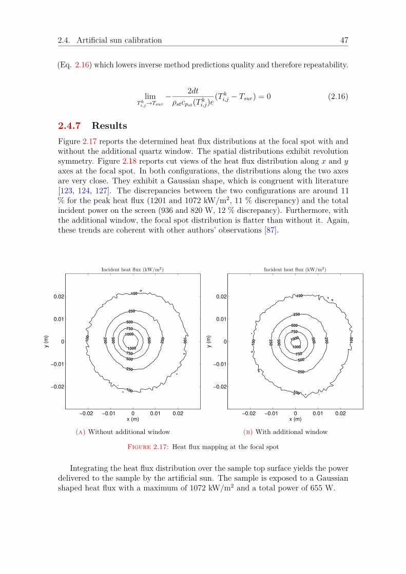
2.4. Artificial sun calibration 47
(Eq. 2.16) which lowers inverse method predictions quality and therefore repeatability.
limT k
i,j→Tsur
− 2dt
ρstcpst(Tki,j)e
(T ki,j − Tsur) = 0 (2.16)
2.4.7 Results
Figure 2.17 reports the determined heat flux distributions at the focal spot with andwithout the additional quartz window. The spatial distributions exhibit revolutionsymmetry. Figure 2.18 reports cut views of the heat flux distribution along x and yaxes at the focal spot. In both configurations, the distributions along the two axesare very close. They exhibit a Gaussian shape, which is congruent with literature[123, 124, 127]. The discrepancies between the two configurations are around 11% for the peak heat flux (1201 and 1072 kW/m2, 11 % discrepancy) and the totalincident power on the screen (936 and 820 W, 12 % discrepancy). Furthermore, withthe additional window, the focal spot distribution is flatter than without it. Again,these trends are coherent with other authors’ observations [87].
x (m)
y (
m)
Incident heat flux (kW/m²)
100
250
500
750
1000
1000
750
500
250
100
500
250
100
2501
00 5
00
−0.02 −0.01 0 0.01 0.02
−0.02
−0.01
0
0.01
0.02
Incident heat flux (kW/m2)
(a) Without additional window
x (m)
y (
m)
Incident heat flux (kW/m²)
100
250
500
750
1000
1000
750
500
250
100
500
250
1005
00
250
100
−0.02 −0.01 0 0.01 0.02
−0.02
−0.01
0
0.01
0.02
Incident heat flux (kW/m2)
(b) With additional window
Figure 2.17: Heat flux mapping at the focal spot
Integrating the heat flux distribution over the sample top surface yields the powerdelivered to the sample by the artificial sun. The sample is exposed to a Gaussianshaped heat flux with a maximum of 1072 kW/m2 and a total power of 655 W.

48 Chapter 2. Materials and methods
−4 −2 0 2 40
250
500
750
1000
1250
Axis length (cm)
Incidentheatflux(kW
/m
2)
(a) Without additional window
−4 −2 0 2 40
250
500
750
1000
1250
Axis length (cm)
Incidentheatflux(kW
/m
2)
(b) With additional window
Figure 2.18: Heat flux distributions at the focal spot. Continuous line: along x axis, dashed line:along y axis
2.4.8 Comments on the calibration method
This calibration method uses inverse methods on a basic level. Using more advancedtechniques, the incident heat flux can be further characterized. Among the criticalpossible improvements, time variability of the heat flux is of note. Indeed using moresophisticated approaches [130, 137, 138], it would be possible to compute a timedependent incident heat flux and convective heat transfer coefficient for each pixel.
Nevertheless, it is thought that the method used here can be trusted. Indeed,the set of results obtained far from the focal spot were validated by comparison withGardon radiometer readings: the agreement between the two methods is very good.Furthermore, the computed beam total power has also been shown to be the samefor several distances of the screen to the focal spot. Finding that total power isconservative is a token of the good quality of the proposed method.
2.5 Experimental procedures
Two different, yet similar, protocols were followed depending on whether or not thecondenser was used.
Without condenser, the following steps were strictly followed for each run:
• drying the porous media upstream of the sample using a dry nitrogen flowuntil its mass stabilised (usually 2 hours)
• weighing of the sample and the reaction chamber

2.5. Experimental procedures 49
• fitting of the sample inside of the reaction chamber
• purging the system with nitrogen
• placing the cell at the focal spot
• starting mass and temperatures recordings
• opening of the shutter
• exposing the sample for 5 min
• closing of the shutter
• cooling the sample under nitrogen sweep for 5 min
• extracting the sample
• weighing the sample and the reaction chamber
• cleaning every part using isopropanol
With the condenser, some specific steps were added:
• drying the porous media upstream of the sample using a dry nitrogen flowuntil its mass stabilised (usually 2 hours)
• weighing the sample, the reaction chamber, the condenser and the cotton trap
• immersing condenser into liquid nitrogen
• fitting of the sample inside of the reaction chamber
• fitting the liquid nitrogen cooled condenser and the cotton trap into the reactionchamber
• purging the system with nitrogen
• placing the cell at the focal spot
• starting mass and temperatures recordings
• opening of the shutter
• exposing the sample for 5 minutes while collecting gas sample
• closing of the shutter
• cooling the sample under nitrogen sweep for 5 min
• extracting the sample and the condenser
• weighing the sample, the reaction chamber, the condenser and the cotton
• placing tar soiled cotton in air tight recipient

50 Chapter 2. Materials and methods
• cleaning every part using isopropanol
In order to assess the run to run repeatability, each run was repeated at leastthree times.
2.6 Data processing
To go from raw data to information, mass and temperature measurements needrefinement. The mass signal processing into wood consumption and also dryingwater release, char gas and tar average production rates is described below. Then,the next step is taken by calculating mass and energy balances.
2.6.1 Gas, tar, water and char final yields
To derive gas, tar, water and char final yields, different parts of the experimentaldevice were weighed before and after a run (Section 2.3.1.4). These measurementsare used to calculate mass variations over a run. Then, these mass variations aredivided by the run time in order to obtain consumption and production rates.
Samples were exposed to radiative power in two configurations: with and withoutcondenser. During a run without the condenser, gas, tar and water freely escaped fromthe reaction chamber. Thus, the reaction chamber mass variation δmchamber, no cond
accounts for the mass of gas produced by the sample mgas, the mass of evaporatedwater from the sample mwater and the mass of tar produced by the sample mtar
(Eq. 2.17).
δmchamber, no cond = mchamber, fin no cond−mchamber, ini no cond = mgas + mwater + mtar
(2.17)During a run with the condenser, gas alone escapes from the reaction chamber.
Thus, the reaction chamber mass variation δmchamber, cond only accounts for the massof gas produced by the sample mgas (Eq. 2.18).
δmchamber, cond = mchamber, fin cond −mchamber, ini cond = mgas (2.18)
The question of the validity of the comparison between δmchamber, no cond andδmchamber, cond may arise. Indeed, these two values are not determined using the samesample. Comparing the reaction chamber mass variation in the two configurations(i.e. δmchamber, no cond and δmchamber, cond) is possible thanks to the good run to runrepeatability of the mass signal (Fig. 2.19).
From these various measurements, it is possible now to determine the mass ofevaporated water released by the sample mwater. First of all, mwood, mchar, msample, ini,msample, fin, mgas and δmchamber, no cond are known. We now consider the samplemass variation δmsample. It accounts for the mass loss of wood mwood, mass loss by

2.6. Data processing 51
0 1 2 3 4 5−30
−20
−10
0
Time (min)
Mass
(g)
Figure 2.19: Six mass signals of reference case samples (9 %wb, bois de bout). Black: withcondenser (stopping tar and water), gray: without condenser
drying mwater and mass gain by char formation mchar (Eq. 2.19). It possible toaccess mwater using Eq. 2.19. By knowing mwater, it is now possible to access mtar
using Eq. 2.20.
δmsample = msample, fin −msample, ini = mchar −mwood −mwater (2.19)
mtar = mchamber, fin no cond −mchamber, ini no cond −mgas −mwater (2.20)
It is therefore possible to calculate the average wood consumption and alsodrying water release, char, gas and tar average production rates by dividing themasses by the total run time of 5 minutes. These time averaged production rates areto be considered with caution. Indeed, one should bear in mind that actual, timedependent, production rates may not be constant over time.
Furthermore, by continuously weighing the reaction chamber during a run withthe condenser, it is possible to monitor the evolution of gas production rate over time.
2.6.2 Mass and energy balances
Knowing the different species production rates, it is easy to derive the mass balanceby comparing gas, tar and char production rates to wood consumption rate. In orderto go further, energy balance is computed.
The considered system is the reaction chamber enclosing the sample. In order tocompute energy balance, it is mandatory to identify energy inlets, outlets, sources,sinks and storages. There are two energy inflows and sources:

52 Chapter 2. Materials and methods
• the incident radiative power
• the chemical power of the pyrolysed wood
Four energy outflows and sinks can be counted:
• the chemical energy stored in gas and tar
• the sensible heat contained in the flue gas
• the water vaporisation heat
• the power emitted by the exposed surface of the sample
The system can store energy in two ways:
• the chemical energy stored in the produced char
• the sensible heat contained in the remains of the sample
Knowing the production rates of the different species, it is possible to calculatethe chemical power contained in their flows using their Higher Heating Value(HHV). Wood, tar and char HHVs were taken from literature with values of 19.0,19.0 and 32.1 MJ/kg respectively [139–141]. Gas HHV was calculated based onits composition using individual species HHV (Table 2.5). Using temperaturemeasurements, the sensible heat contained in the flue gas and the remains of thesample can be evaluated. Sensible heat evaluation requires to know the specificheat capacity of the flue gas and the remains of the sample. Those were esti-mated, as the nitrogen specific heat capacity at the flue gas temperature for theflue gas, and as the wood specific heat capacity at 50 °C for the remains of the sample.
Species HHV (MJ/kg)
Beech wood 19.0Tar 19.0Char 32.1H2 142CO 10.1CO2 0CH4 55.5C2H2 49.9C2H4 50.3C2H6 51.9C3H8 50.4
Table 2.5: Species Higher Heating Value (HHV) [139–142]
Evaluating the radiative heat loss is more challenging. The power emitted by thesample (Prad,loss) can be estimated using Eq. 2.21. Yet, one needs to determine thesurface and the temperature of the power emitting area. The temperature is taken as
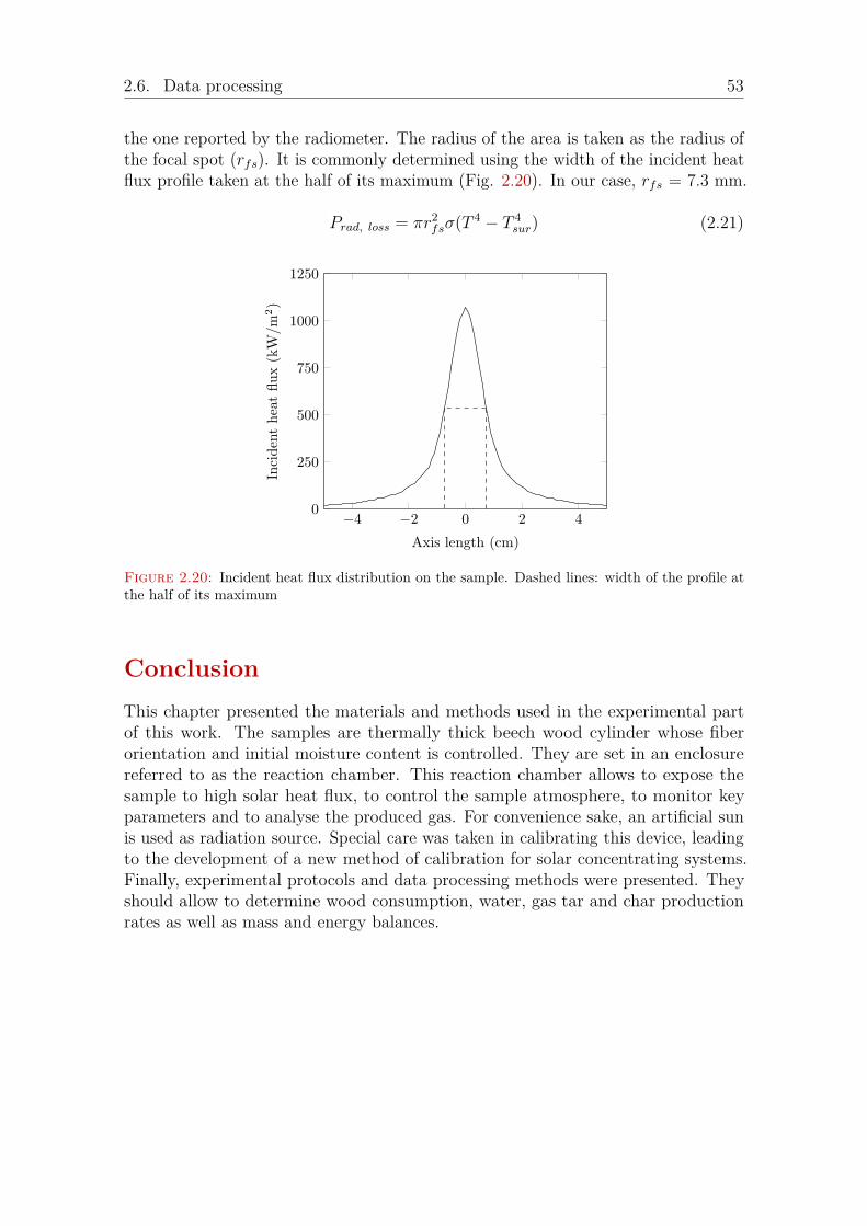
2.6. Data processing 53
the one reported by the radiometer. The radius of the area is taken as the radius ofthe focal spot (rfs). It is commonly determined using the width of the incident heatflux profile taken at the half of its maximum (Fig. 2.20). In our case, rfs = 7.3 mm.
Prad, loss = πr2fsσ(T 4 − T 4
sur) (2.21)
−4 −2 0 2 40
250
500
750
1000
1250
Axis length (cm)
Incidentheatflux(kW
/m
2)
Figure 2.20: Incident heat flux distribution on the sample. Dashed lines: width of the profile atthe half of its maximum
Conclusion
This chapter presented the materials and methods used in the experimental partof this work. The samples are thermally thick beech wood cylinder whose fiberorientation and initial moisture content is controlled. They are set in an enclosurereferred to as the reaction chamber. This reaction chamber allows to expose thesample to high solar heat flux, to control the sample atmosphere, to monitor keyparameters and to analyse the produced gas. For convenience sake, an artificial sunis used as radiation source. Special care was taken in calibrating this device, leadingto the development of a new method of calibration for solar concentrating systems.Finally, experimental protocols and data processing methods were presented. Theyshould allow to determine wood consumption, water, gas tar and char productionrates as well as mass and energy balances.


CHAPTER 3Experimental results
Introduction . . . . . . . . . . . . . . . . . . . . . . . . . . . . . . 56
3.1 Reference case processing . . . . . . . . . . . . . . . . . . 56
3.1.1 Experimental observations . . . . . . . . . . . . . . . . . . 56
3.1.2 Char properties . . . . . . . . . . . . . . . . . . . . . . . . 61
3.2 Crater formation . . . . . . . . . . . . . . . . . . . . . . . . 64
3.3 Impact of fiber orientation . . . . . . . . . . . . . . . . . . 66
3.4 Impact of initial moisture content . . . . . . . . . . . . . 68
3.5 Energy balance . . . . . . . . . . . . . . . . . . . . . . . . . 71
Conclusion . . . . . . . . . . . . . . . . . . . . . . . . . . . . . . . 73
55
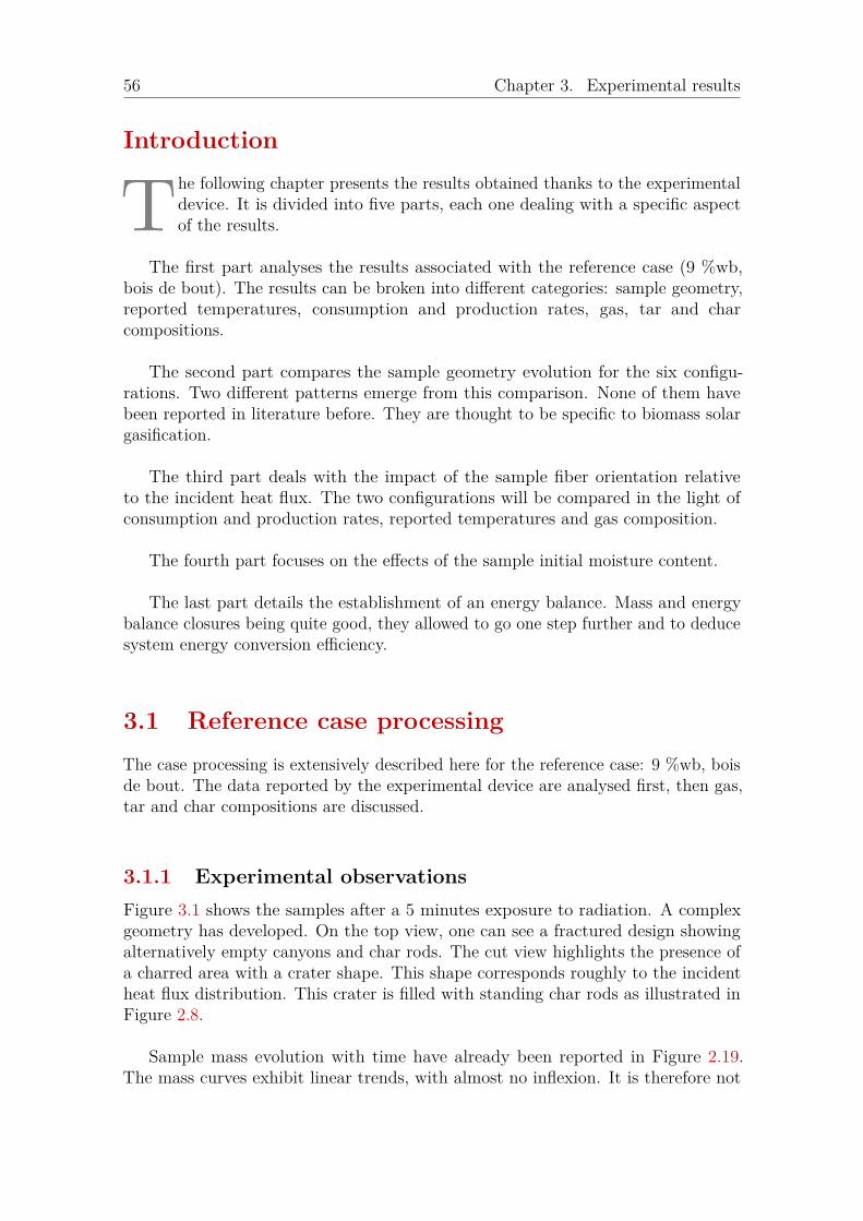
56 Chapter 3. Experimental results
Introduction
The following chapter presents the results obtained thanks to the experimentaldevice. It is divided into five parts, each one dealing with a specific aspectof the results.
The first part analyses the results associated with the reference case (9 %wb,bois de bout). The results can be broken into different categories: sample geometry,reported temperatures, consumption and production rates, gas, tar and charcompositions.
The second part compares the sample geometry evolution for the six configu-rations. Two different patterns emerge from this comparison. None of them havebeen reported in literature before. They are thought to be specific to biomass solargasification.
The third part deals with the impact of the sample fiber orientation relativeto the incident heat flux. The two configurations will be compared in the light ofconsumption and production rates, reported temperatures and gas composition.
The fourth part focuses on the effects of the sample initial moisture content.
The last part details the establishment of an energy balance. Mass and energybalance closures being quite good, they allowed to go one step further and to deducesystem energy conversion efficiency.
3.1 Reference case processing
The case processing is extensively described here for the reference case: 9 %wb, boisde bout. The data reported by the experimental device are analysed first, then gas,tar and char compositions are discussed.
3.1.1 Experimental observations
Figure 3.1 shows the samples after a 5 minutes exposure to radiation. A complexgeometry has developed. On the top view, one can see a fractured design showingalternatively empty canyons and char rods. The cut view highlights the presence ofa charred area with a crater shape. This shape corresponds roughly to the incidentheat flux distribution. This crater is filled with standing char rods as illustrated inFigure 2.8.
Sample mass evolution with time have already been reported in Figure 2.19.The mass curves exhibit linear trends, with almost no inflexion. It is therefore not

3.1. Reference case processing 57
(a) Top view (b) Cut view
Figure 3.1: Sample views after a 5 minutes exposure for the reference case (9 %wb, bois de bout)
possible to identify phenomena at stake from mass readings. Yet, these curves canbe processed to yield averaged production/consumption rates.
On average, wood consumption rate is 5.76 g/min (Table 3.1). It is mainlytransformed into gas (3.65 g/min) and char (1.37 g/min). The production oftar is quite low with only 9 % (0.50 g/min) of the dry wood being turned intotar. This low tar yield is later explained by tar thermal cracking and steam reforming.
Radiometer surface temperature measurements are reported in Figure 3.2. Duringthe first few seconds of the run, the reading exhibits an overshoot. This overshootis explained by the high reflectivity of virgin wood around 63 % [109] that blindsthe radiometer with reflected light from the xenon arc lamp. Once the surface ischarred, the reflectivity drops to near zero and allows for a proper measurement ofthe surface temperature. During a run, surface temperature is around 1530 °C, witha slightly downward trend. Between runs, measurements exhibit the same trend, yet± 120 °C variations are observed. It is known from literature that temperatureshigher than 800 °C are required to achieve tar thermal cracking [75] and tar steamreforming [76]. Here, the reported temperature is much higher than 800 °C, makingtar thermal cracking and tar steam reforming kinetically favoured.
Figure 3.3 presents in depth thermocouple temperature measurements. Thesemeasurements show a wide run to run variation. Indeed, thermocouples are locatedin a fractured medium. Depending on the thermocouple location, i.e. inside achar rod or in between two rods, the reported temperatures differ. When locatedin between two rods, the thermocouple is directly exposed to the incident heat,therefore its temperature increases sharply. When concealed inside of a char rod, thetemperature history shows a plateau around 100 °C, associated to drying, and thensteadily increases. Nevertheless, it yields some information on the sample heatingrate. From thermocouple inside a rod readings, heating rate inside of the sample is

58 Chapter 3. Experimental results
Tim
eav
eragedrate
(g/min
)T
emp
erature
Wood
Water
Char
Gas
Tar
(°C)
Bois
de
bou
t
0%
wb
7.05±
0.480.49
±0.49
1.74±
0.0024.12
±0.07
1.63±
0.88
1594±
1239
%w
b5.76
±0.42
1.57±
0.431.37
±0.002
3.65±
0.07
0.50±
0.82
1530±
12055
%w
b0.99
±0.02
5.89±
0.060.09
±0.002
1.70±
0.55
-0.8
7±
0.93
1317±
98
Bois
de
fil
0%
wb
7.09±
0.480.06
±0.49
1.48±
0.0023.64
±0.1
91.8
4±
0.981616
±46
9%
wb
5.68±
0.421.09
±0.42
1.38±
0.0023.58
±0.2
30.4
9±
0.831605
±90
55%
wb
1.49±
0.032.57
±0.04
0.17±
0.0021.94
±0.2
0-0.80
±0.98
1426±
20
Ta
ble
3.1:T
ime
avera
ged
wood
consu
mptio
n,
water,
char,
gasan
dtar
pro
duction
ratesan
daverage
surface
temp
erature
forth
esix
configu
rations
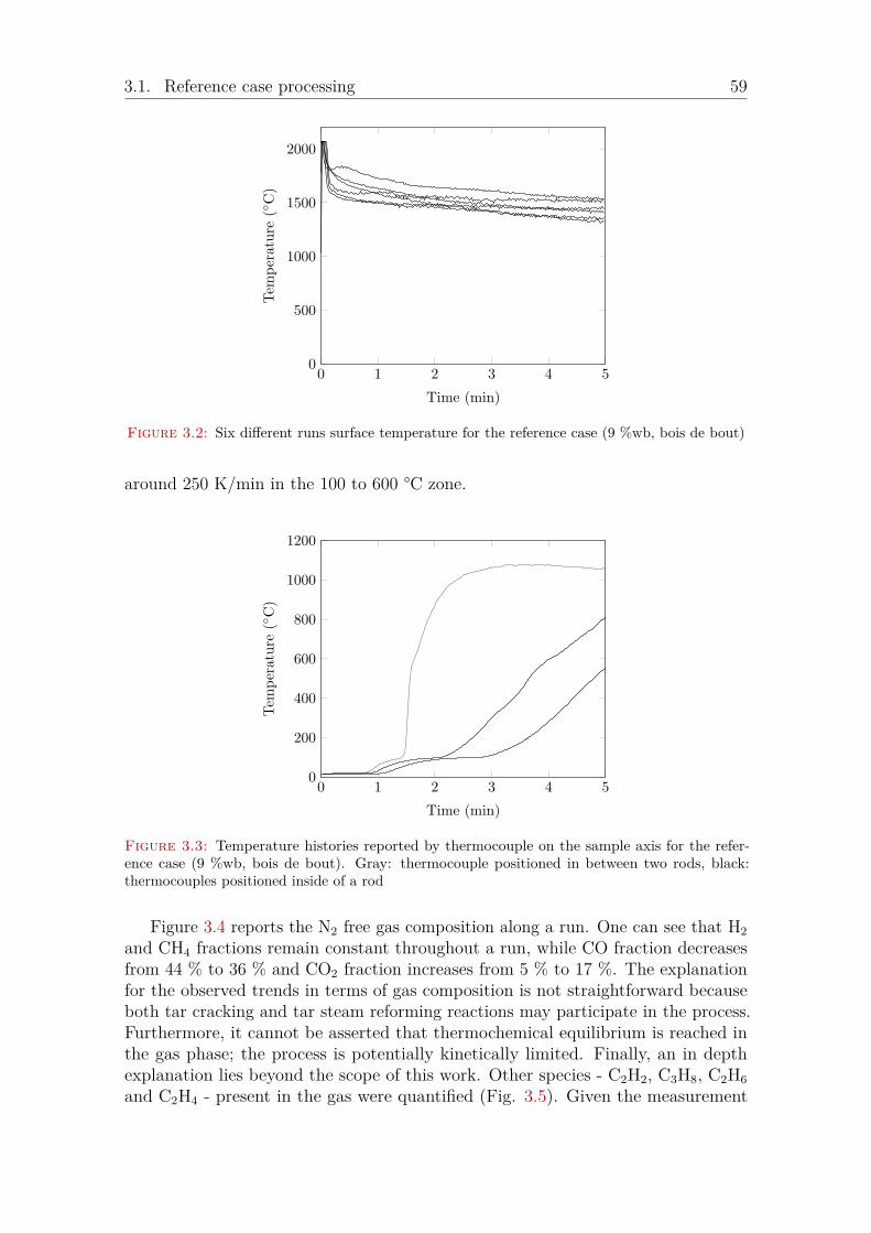
3.1. Reference case processing 59
0 1 2 3 4 50
500
1000
1500
2000
Time (min)
Tem
perature
(◦C)
Figure 3.2: Six different runs surface temperature for the reference case (9 %wb, bois de bout)
around 250 K/min in the 100 to 600 °C zone.
0 1 2 3 4 50
200
400
600
800
1000
1200
Time (min)
Tem
perature
(◦C)
Figure 3.3: Temperature histories reported by thermocouple on the sample axis for the refer-ence case (9 %wb, bois de bout). Gray: thermocouple positioned in between two rods, black:thermocouples positioned inside of a rod
Figure 3.4 reports the N2 free gas composition along a run. One can see that H2
and CH4 fractions remain constant throughout a run, while CO fraction decreasesfrom 44 % to 36 % and CO2 fraction increases from 5 % to 17 %. The explanationfor the observed trends in terms of gas composition is not straightforward becauseboth tar cracking and tar steam reforming reactions may participate in the process.Furthermore, it cannot be asserted that thermochemical equilibrium is reached inthe gas phase; the process is potentially kinetically limited. Finally, an in depthexplanation lies beyond the scope of this work. Other species - C2H2, C3H8, C2H6
and C2H4 - present in the gas were quantified (Fig. 3.5). Given the measurement

60 Chapter 3. Experimental results
uncertainty, their fractions can be considered stable during a run. Gas readings showa good repeatability from run to run. Therefore, the averaged total gas productionrate was computed from the average gas composition. The obtained values are 10% close to the one obtained using mass measurements. It is thought to be a verysatisfactory agreement.
0 1 2 3 4 50
10
20
30
40
50
CO
H2
CH4
CO2
Time (min)
Fraction(%
vol)
Figure 3.4: Gas composition downstream the condenser for the reference case (9 %wb, bois debout), major species. Triangle: H2, circle: CO, diamond: CO2, square: CH4
0 1 2 3 4 50
1
2
3
C2H4
C2H2
C3H8
C2H6
Time (min)
Fraction(%
vol)
Figure 3.5: Gas composition downstream the condenser for the reference case (9 %wb, bois debout), minor species. Triangle: C3H8, circle: C2H6, diamond: C2H4, square: C2H4
Tar analyses show that they are mainly composed of primary (acetic acid, phenol,hydroxyethanal, 1-hydroxy-2-propanone) and tertiary (naphthalene, acenaphthalene,phenanthrene) organic tar [74] (Appendix A). This configuration, where primaryand tertiary tar are found together with no significant amount of secondary tar, isknown to be a sign of intense thermal cracking [75]. Furthermore, the analyses show

3.1. Reference case processing 61
a good run to run repeatability even though tar were stored for a long time beforebeing analysed.
Until now, we only considered time averaged value of production rates. Theexperimental device allows to go one step further and study the gas productionrate evolution with time. Gas production rates for the reference case is available inFigure 3.6. Gas production clearly increases with time. It is thought that as thechar crater grows the residence time of tars inside of it increases. Therefore, thecontact time between steam and tar before quenching by nitrogen sweep increases,favouring tar thermal cracking and tar steam reforming leading to gas formation.
0 1 2 3 4 50
1
2
3
4
5
Time (min)
Productionrate
(g/min)
Figure 3.6: Gas production rate for the reference case (9 %wb, bois de bout) with estimated errorbars
3.1.2 Char properties
In order to get more insight on char composition and structure, char rods were takenfrom the sample and ground. Nevertheless, one should keep in mind that the charmay not be homogeneous throughout the sample. Therefore, obtained results reflectaverage char properties.
Table 3.2 reports the ultimate analysis for char obtained from bois de bout withdifferent initial moisture content. These char compositions are similar. They allexhibit high oxygen and hydrogen contents. Oxygen fractions can be as high as18.11 % for 55 %wb initial moisture content sample. Yet, these results are in goodagreement with the existing study on solar pyrolysis [25]. High oxygen and hydrogenfractions of are signs that these chars have not undergone thermal annealing [46]even though they were produced at high temperature. It might be explained by thefact that the char does not spend enough time at high temperature to undergo asignificant amount of annealing.

62 Chapter 3. Experimental results
Wood initial moisture content 0 %wb 9 %wb 55 %wb
Carbon 85.06 87.82 78.5Hydrogen 2.94 2.75 3.05Oxygen 11.99 9.43 18.11Nitrogen - - 0.34Sulphur - - -
Table 3.2: Char ultimate analysis (%wt)
A TriStar II 3020 BET was used to determine the chars specific surface areaand pore volume (Table 3.3). These values are in good agreement with literature[25]. Furthermore, two trends emerge from these measurements: a higher initialmoisture content leads to higher specific surface area and pore volume and bout de filconfigurations exhibit higher specific surface area and pore volume than bois de boutconfigurations. The first trend can be explained by the fact that high initial moisturecontent enables char steam gasification to a higher extent than low initial moisturecontent cases. Gasification turns char into gas, and hence increases the specificsurface area and pore volume. Thus a higher amount of char steam gasificationinduces a higher specific surface area and pore volume. Regarding the impact offiber orientation, it can be noted that in bois de fil configurations, gases escape bythe rear of the char rods while they escape by the top of the rods in bois de boutconfigurations. Hence, the residence time of tar inside of the rods is shorter in boutde fil configurations than in bois de bout configurations. Thus, less time is offeredto tar repolymerisation reactions, carbon deposit is therefore less important whichleads to higher surface area and pore volume.
Specific surface area (m2/g) Pore volume (cm3/g)
Bois debout
0 %wb 44.13 0.011509 %wb 76.56 0.0241555 %wb 86.61 0.04905
Boisde fil
0 %wb 93.16 0.040879 %wb 69.86 0.0305355 %wb 122.38 0.08774
Table 3.3: Chars BET specific surface area and BJH adsorption pore volume
The structure of a char rod was also analysed using scanning electron microscope(SEM) (Fig. 3.7). From the top view, one can see that the char has kept the woodchannel structure. Special structures can be found at the end of these channels.They look like solidified liquid. They are thought to be intermediate liquid compound[22, 56], that was molten during the run and that solidified during the samplecooling. On the side view, it is possible to see minerals (white dots) uniformly spreadthroughout the surface.
Finally, char spectral properties have already been reported in Section 2.2.2.

3.1. Reference case processing 63
(a) Top view
(b) Side view
Figure 3.7: Char rod SEM pictures for the reference case (9 %wb, bois de bout)
They are in good agreement with values found in literature.

64 Chapter 3. Experimental results
3.2 Crater formation
Top and cut views of 0, 9 and 55 %wb initial moisture content samples in both fiberdirections are reported in Figures 3.8 and 3.9. The 0 %wb initial moisture contentsamples cut views are close to those of 9 %wb initial moisture content samples.During a run, sample geometry is significantly modified. Two main behavioursemerge from these observations. For low initial moisture content samples, char rodsstand inside the crater. For high initial moisture content samples, a smaller crater isformed, yet no rods stand inside of it. Moreover, cut views show that the transitionbetween wood and char is very sharp. It is therefore possible to consider that thesides of the crater are in fact the location of a pyrolysis front. Sadly, no transitionbetween wet and dry wood can be observed. Thus, it is not possible to locate apotential drying front.
In the case of low initial moisture content samples, wood shrinkage and mechanicalfailure are thought be at the origin of the char rods formation. Indeed, it is knownthat during pyrolysis wood shrinks as it turns into char loosing about 65 % ofits initial volume [108, 109]. In this case, under radiative heat flux, the mediumundergoes pyrolysis and starts shrinking. As the mechanical constraint grows, someweak spots in the wood structure break. These breaks yield char rods on one handand canyons on the other. Then the canyons allow the radiation to penetrate evenfurther inside of the sample, providing energy for in depth pyrolysis. In the end,this mechanism yields a crater zone which has a shape close to incident heat fluxdistribution. Moreover, it is possible using the cut view pictures to determine thepyrolysis front thickness. The front thickness is about 4 mm for 0 %wb samples and3 mm for 9 %wb samples
In the case of high initial moisture content samples, steam coming from drying isthought to play a major role in the geometrical evolution of the sample. In the caseof low initial moisture content samples, the amount of water released by drying isnot high enough to allow for complete char gasification. For high initial moisturecontent samples, the drying provides enough steam to gasify the char producedby the pyrolysis. Indeed, in order to escape from the sample, the steam has to gothrough the char which is at a temperature far higher than 800 °C. Therefore, charundergoes steam gasification which explains why no char rods are found inside of thecrater. Furthermore, the pyrolysis front thickness is small, about 0.5 mm. Indeed,pyrolysis is thought to be shortly preceded by a drying front and is closely followed bya gasification front which immediately consumes the char produced by the pyrolysisfront
There are also similarities in the crater shapes between bois de bout and boisde fil sample (Fig. 3.9). In the case of 0 and 9 %wb initial moisture samples, thechar rods inside of the crater are standing upward in both cases. This is surprisinggiven the fact that in the bois de fil cases, the wood fibers are orthogonal to theincident heat flux. Nevertheless, some minor discrepancies remain. One can alsonote that the average diameter of the char rods is more important for bois de filsamples. Bois de bout samples exhibit a deeper and narrower crater than bois de filsamples. This is due to the fact that wood is an anisotropic material. In the boisde bout cases, the fiber orientation favours heat conduction towards the bottom of

3.2. Crater formation 65
(a) 0 %wb bois de bout (b) 0 %wb bois de fil
(c) 9 %wb bois de bout (d) 9 %wb bois de fil
(e) 55 %wb bois de bout (f) 55 %wb bois de fil
Figure 3.8: Sample top views after 5 minutes exposure

66 Chapter 3. Experimental results
(a) 0 %wb bois de bout (b) 0 %wb bois de fil
(c) 9 %wb bois de bout (d) 9 %wb bois de fil
(e) 55 %wb bois de bout (f) 55 %wb bois de fil
Figure 3.9: Sample cut views after 5 minutes exposure
the crater inducing sharper shapes. In the bois de fil cases, the fiber orientationfavours heat conduction towards the sides of the crater inducing flatter shapes. Charinternal geometry also differs between the two configurations. As aforementioned,bois de fil samples exhibits higher specific surface area and pore volume than bois debout samples (Table 3.3).
3.3 Impact of fiber orientation
Sample fiber orientation varies between two extreme configurations: bois de bout(vertical fibers) and bois de fil (horizontal fibers). This difference was expected tohave an impact on the behaviour of the samples because wood is an anisotropicmaterial. Indeed, the ratio of longitudinal to radial thermal conductivity is about 2[143] and the ratio of the permeability for the same directions is about five thousand[34].
Figure 3.10 allows for a direct confrontation of the production/consumption ratesbetween the two fiber orientations (data can be found in Table 3.1). The woodconsumption, drying water release, gas, tar and char production rates exhibit closevalues with only one exception for the 55 %wb cases. In these particular cases, waterreleased is much higher for vertical fiber samples than for horizontal ones. It can be

3.3. Impact of fiber orientation 67
explained by the fact that these saturated samples dry in pure nitrogen. Indeed, thechannels of the wood come out directly on a dry nitrogen sweeping flow. This setupdramatically promotes drying. In the case of bois de fil samples, the channels of thewood come out on the side of the sample, where there is no sweep. The discrepancybetween bois de bout and bois de fil water release rate for 55 %wb samples isexplained by a more efficient drying in the first case. This was checked in special ex-periments where samples were expose to the nitrogen sweep without radiative heating.
Wood Water Char Gas Tar0
2
4
6
8
Production/con
sumption
rate
(g/m
in)
0 %wb
9 %wb
55 %wbBois de boutBois de fil
Figure 3.10: Production/consumption rates for the six configurations
Figure 3.11 reports the fractions of the major components of the gas at the outletof the condenser (data can be found in Table 3.4). The gas composition for the twofiber orientations are very close for CO, CO2 and CH4. The fraction of H2 may seemto be slightly more important for bois de fil, yet, given the uncertainty, no solidconclusion can be drawn. The same can be stated for minor gas components asreported in Table 3.5.
Finally, average surface temperatures are very close for bois de bout and bois defil configurations (Table 3.1).

68 Chapter 3. Experimental results
H2 CO CO2 CH4
0
10
20
30
40
50
Fraction(%
vol)
Bois de boutBois de fil
Figure 3.11: Fractions of major components in the gas for 9 %wb moisture content samples. Darkgray: bois de bout, light gray: bois de fil
Fraction (%vol)H2 CO CO2 CH4
Bois debout
0 %wb 25.85 ± 2.06 43.16 ± 2.37 11.09 ± 2.59 13.22 ± 0.539 %wb 27.79 ± 2.31 39.88 ± 2.13 9.45 ± 2.29 11.63 ± 0.4455 %wb 37.81 ± 3.42 30.95 ± 3.12 12.15 ± 2.41 8.47 ± 0.95
Boisde fil
0 %wb 30.52 ± 3.32 40.53 ± 1.17 11.23 ± 2.01 11.23 ± 0.499 %wb 31.35 ± 0.89 40.01 ± 3.04 11.78 ± 2.81 10.76 ± 0.7555 %wb 36.83 ± 1.69 33.42 ± 2.36 13.51 ± 2.13 8.71 ± 0.53
Table 3.4: Fractions of major components in the N2 free gas at the outlet of the condenseraveraged throughout a run
Fraction (%vol)C2H2 C3H8 C2H6 C2H4
Bois debout
0 %wb 1.69 ± 0.48 0.31 ± 0.13 0.34 ± 0.05 2.73 ± 0.299 %wb 1.41 ± 0.28 0.27 ± 0.08 0.26 ± 0.06 2.29 ± 0.3155 %wb 1.70 ± 0.38 0.03 ± 0.02 0.11 ± 0.02 1.80 ± 0.32
Boisde fil
0 %wb 1.33 ± 0.19 0.20 ± 0.08 0.32 ± 0.05 2.26 ± 0.399 %wb 1.58 ± 0.51 0.22 ± 0.11 0.29 ± 0.04 2.08 ± 0.2055 %wb 1.65 ± 0.26 0.10 ± 0.05 0.20 ± 0.03 1.97 ± 0.12
Table 3.5: Fractions of minor components in the N2 free gas at the outlet of the condenseraveraged throughout a run
3.4 Impact of initial moisture content
The comparison of production/consumption rates between different initial moisturecontents cases is not direct. For instance, the amount of gas produced by a highinitial moisture sample is lower than for an initially dry sample. Yet, the amount ofconverted wood is not the same between these two. In order to solve this problem,

3.4. Impact of initial moisture content 69
the water, char, gas and tar production rates were divided by the wood consumptionrate, giving yields on dry wood basis (Table 3.6).
Water Char Gas Tar Closure (%)
Bois debout
0 %wb 0.07 ± 0.07 0.25 ± 0.02 0.58 ± 0.05 0.23 ± 0.14 1069 %wb 0.27 ± 0.09 0.24 ± 0.02 0.63 ± 0.06 0.09 ± 0.15 9655 %wb 5.97 ± 0.20 0.09 ± 0.01 1.73 ± 0.60 -0.89 ± 0.93 105
Boisde fil
0 %wb 0.01 ± 0.07 0.21 ± 0.01 0.51 ± 0.06 0.26 ± 0.16 989 %wb 0.19 ± 0.09 0.24 ± 0.02 0.63 ± 0.09 0.09 ± 0.15 9655 %wb 1.73 ± 0.07 0.11 ± 0.01 1.31 ± 0.17 -0.54 ± 0.65 88
Table 3.6: Time averaged yields on dry wood basis and mass closure
Firstly, as one can see from Table 3.6, the closure of the mass balance is between88 and 106 % which is quite good. Then, as stated before, fiber orientation inducesonly minor variations in terms of yields. Figure 3.12 reports the relative productionyields for bout de fil samples; two main trends emerge from these results:
0 10 20 30 40 500
0.5
1
1.5
2
Initial moisture content (%wb)
Relativeproductionrate
Figure 3.12: Relative production rate for bout de fil samples over the range of initial moisturecontent. Triangle: drying water, square: char, circle: gas, diamond: tar
• an increase in sample initial moisture content leads to a significant reductionof tar production. For 0 %wb initial moisture content samples, about 25 % ofthe wood is transformed into tar. Whereas the tar yield is only 9 % for 9 %wbinitial moisture content samples. Tar steam reforming is thought to play arole in this reduction. Indeed, both tar and steam have to escape the mediumpassing through the crater where temperature is high enough to promote tarsteam reforming
• an increase in sample initial moisture content leads to a major increase in gasproduction, relative to the wood consumption. The gas yield even exceeds 1 for

70 Chapter 3. Experimental results
55 %wb initial moisture content samples. This means that the produced gasmass exceeds the consumed dry wood mass. It is possible if steam contributesto gas mass through char steam gasification, tars or methane steam reforming
The reported tar production rates are negative for 55 %wb initial moisturecontent samples (Table 3.1). The error associated with these measurements is quitehigh. Two observations are to be added. It has been qualitatively observed thattar production during these runs is actually very low. Indeed, at the end of theseruns the condenser contains only water; no sign of tar (in terms of deposit, color norsmell) can be found in it. Furthermore, the tar cotton trap is superficially colouredin light brown, suggesting that only few tars were produced and trapped.
As one can see in Figure 3.13, gas composition varies with sample initial moisturecontent. Given the error bars, it is possible to consider that gas from 0 and 9 %wbinitial moisture content samples have the same composition. Increasing the initialmoisture content to 55 %wb leads to an increase in H2 fraction from 26 to 38 %vol,a decrease in CO and CH4 fractions from 43 to 31 %vol and from 13 to 8.5 %volrespectively, while CO2 fractions remains stable. Yet, one should keep in mindthat the total gas mass production dramatically increases at the same time. Therise in H2 production is thought to be associated with syngas production by steamgasification of char.
H2 CO CO2 CH4
0
10
20
30
40
50
Fraction(%
vol)
0 %wb
9 %wb
55 %wb
Figure 3.13: Major components of the gas for 0, 9 and 55 %wb moisture content bois de boutsamples
Tar captured in cotton traps were analysed for 0 and 9 %wb initial moisture boisde bout samples. It was not possible to analyse tar produced by 55 %wb initialmoisture content samples. Indeed, as aforementioned, the cotton traps containedalmost no tar. Analysed tar compositions are similar. In the two configurations,the main products are primary and tertiary tar which are indicators of intense tarthermal cracking. Yet, 0 %wb initial moisture content sample tars exhibit a slightlywider variety of PAH. Steam reforming takes place to a greater exten for 9 % initialmoisture content samples, which might explain the reduction in number of PAH

3.5. Energy balance 71
found in 9 %wb initial moisture content sample cotton traps.
Finally, average surface temperatures drops from about 1600 °C down to 1300 °Cas biomass initial moisture content increases from 0 to 55 %wb (Table 3.1). This isthought to be a consequence of the endothermic char steam gasification reaction.
3.5 Energy balance
Energy balance of the system was calculated based on the method described inSection 2.6.2. In order to evaluate specific heat capacities and powers, it is mandatoryto know the temperatures of the flue gas, the focal spot and the sample. Flue gastemperature was taken as 150 °C, in agreement with thermocouples measurements.Radiometer reported temperatures were used to calculate sample emitted power.Sample sensible heat is more challenging to evaluate. Indeed, temperature is notuniform throughout the sample. It was chosen to rely the pre-model predictions aswell as thermocouple readings. Therefore, the sample sensible heat was determinedconsidering a 250 g sample of which average temperature is about 50 °C. Table 3.7reports the values of the different contributions to the energy balance as well asclosure of this balance. The closure of the energy balance ranges from 87 to 104 %which is thought to be satisfactory.
Considering that at the process scale, gas, tar and char are the recoverable outputenergy carriers, it is interesting to evaluate the fraction of the input energy theseproducts can contain. We consider the two energy inputs - incident radiative powerand chemical power contained in wood - and the three energy outputs - chemicalpowers contained in gas, tar and char. Table 3.8 provides the fraction of the inputpower sources transferred to the three outputs for the six configurations. One cansee that the total power contained in the outputs ranges as high as 94 % for drysamples down to 59 % for high initial moisture content samples. Gas contain about45 % of the input power in any of the configurations. For high initial moisturecontent sample, the output power is only around half of the input power. It is indeedhindered by drying endothermicity.
For the six configurations, the total power contained in the outputs is higher thanthe wood input power, meaning that a fraction of the incident radiative power wasconverted into chemical form. The amount of converted radiative power is calculatedby subtracting the wood HHV input from the total HHV output. Table 3.9 reportsthe amount of radiative power retained by the system outputs. The fraction of theinput radiative power converted into chemical form ranges from 24 % for 9 %wb,bois de fil samples to 72 % for 0%wb, bois de bout samples. Furthermore, as for theenergy conversion efficiency, bois de bout samples exhibit better performances thanbois de fil samples.
Finally, in order to generalize the produced results, the wood consumption, water,char, gas and tar production rates for 1 kW of radiative power were calculated and

72 Chapter 3. Experimental results
Rad
iative
Wood
Gas
Tar
Char
Em
ittedW
aterF
lue
gas
Sam
ple
Closu
rein
put
HH
VH
HV
HH
VH
HV
pow
ervap
orisation
sensib
lesen
sible
(%)
(W)
input
(W)
outp
ut
(W)
outp
ut
(W)
outp
ut
(W)
(W)
pow
er(W
)hea
t(W
)heat
(W)
Bois
de
bou
t
0%
wb
6552233
1254517
93311
618
101
38103
9%
wb
6551825
1137159
73210
159
99
3894
55%
wb
655312
5290
4961
222
104
38104
Bois
de
fil
0%
wb
6552246
1095584
79212
22
99
3894
9%
wb
6551798
1066154
73811
941
98
3892
55%
wb
655470
5760
8980
9797
38
87
Ta
ble
3.7:In
puts
pow
ersdistrib
ution
betw
eench
emical
outp
uts
and
losses

3.5. Energy balance 73
Gas HHV Tar HHV Char HHV Sumoutput (%) output (%) output (%) (%)
Bois debout
0 %wb 43 18 32 949 %wb 46 6 30 8255 %wb 55 0 5 60
Boisde fil
0 %wb 38 20 27 859 %wb 43 6 30 8055 %wb 51 0 8 59
Table 3.8: Power distribution in system chemical outputs. All percentages are on a total powerinput basis (radiative + wood)
Radiative Wood HHV Total HHV Converted radiative Converted radiativeinput (W) input (W) output (W) power (W) power fraction (%)
Bois debout
0 %wb 655 2233 2704 471 729 %wb 655 1825 2028 203 3155 %wb 655 312 578 266 41
Boisde fil
0 %wb 655 2246 2471 225 349 %wb 655 1798 1958 160 2455 %wb 655 470 665 195 30
Table 3.9: Stored radiative power in the system outputs
Initial moisture Production/consumption rate (g/min/kW)content Wood Water Char Gas Tar
0 %wb 10.8 ± 0.73 0.41 ± 0.74 2.46 ± 0 5.92 ± 0.2 2.65 ± 1.429 %wb 8.73 ± 0.64 2.03 ± 0.65 2.1 ± 0 5.52 ± 0.23 0.76 ± 1.2655 %wb 1.89 ± 0.04 6.46 ± 0.07 0.2 ± 0 2.78 ± 0.58 -1.28 ± 1.46
Table 3.10: Averaged wood consumption, water, char, gas and tar production rates per unit ofincident power
reported in Table 3.10 for the different initial moisture contents. This approachshould facilitate reactor design for instance. These data were produced by averagingbois de bout and bois de fil contributions because in a reactor samples are generallyrandomly oriented. In addition, the total outputs power is 90, 81 and 60 % of thetotal inputs power for 0, 9 and 55 %wb initial moisture content samples, respectively.
Conclusion
Thermally thick beech wood samples were exposed to radiative heat flux comparableto the ones found in solar power towers. To do so, a new experimental device wasbuilt. It allowed to investigate the behaviours of the biomass under heat fluxes

74 Chapter 3. Experimental results
higher than 1000 suns.
An original behaviour has been highlighted. Under high radiative heat flux,sample geometry evolves dramatically during a run. A crater which mirrors incidentheat flux distribution is formed. Two mechanisms of crater formation have beenproposed: one involving sample shrinkage and mechanical failure for low initialmoisture content samples, the other relying on char steam gasification for high initialmoisture content samples.
It was shown that, even for high initial moisture content sample, water vaporisa-tion did not suffice to lead to sample mechanical failure. Furthermore, producedchars do not undergo thermal annealing and exhibit high oxygen and hydrogencontents. Finally, achieved temperatures were high enough to promote tar thermalcracking, but not sufficient to induce carbon sublimation.
The effect of wood fiber orientation relative to the incident heat flux wasquestioned. Samples in bois de bout and bois de fil were used to address thisquestion. Surprisingly, the produced results show that varying the sample orientationbetween these two extrema has only a minor effect on the sample behaviour.
The influence of the sample initial moisture content was investigated. It washighlighted that samples containing high initial moisture content undergo chargasification. They produce 2.6 times more gas - per unit of converted dry wood- than low initial moisture content samples. Furthermore, this gas is richer inH2 - 36 %vol instead of 26 %vol. Nevertheless, the input power retained in theproducts is quite low, around 59 %. The tar yield is close to zero. It has alsobeen shown that samples containing no water produce much more tar than moistsamples. For these samples solar pyro-gasification exhibits a very good energyconversion efficiency: the recoverable products contain 90 % of the inputs (solar +wood) power. Furthermore, the power recovered in the outputs exceeds the woodinput power alone, in every configuration. It means that some of the incidentradiative power has been converted into chemical form. The fraction of the inci-dent radiative power captured can be as high as 72 % for 0 %wb, bois de bout samples.
It can be concluded that the solar pyro-gasification of moist biomass is interestingfor enhanced direct H2 production with reduced tar yield, while solar pyro-gasificationof dry biomass is advantageous in the perspective of solar to fuel conversion.
Furthermore, this experimental work yields substantial data which can be usedto validate numerical model predictions.

CHAPTER 4Numerical model
Introduction . . . . . . . . . . . . . . . . . . . . . . . . . . . . . . 76
4.1 Objectives . . . . . . . . . . . . . . . . . . . . . . . . . . . . 77
4.2 Phenomena at stake . . . . . . . . . . . . . . . . . . . . . . 77
4.3 Dimensionless numbers and assumptions . . . . . . . . . 78
4.3.1 Dimensionless numbers . . . . . . . . . . . . . . . . . . . 78
4.3.2 Assumptions . . . . . . . . . . . . . . . . . . . . . . . . . 80
4.4 Numerical model . . . . . . . . . . . . . . . . . . . . . . . . 82
4.4.1 Computational domain . . . . . . . . . . . . . . . . . . . 82
4.4.2 Governing equations . . . . . . . . . . . . . . . . . . . . . 83
4.4.3 Drying model . . . . . . . . . . . . . . . . . . . . . . . . . 86
4.4.4 Biomass degradation scheme . . . . . . . . . . . . . . . . 86
4.5 Physical properties . . . . . . . . . . . . . . . . . . . . . . 88
4.5.1 Solid phases . . . . . . . . . . . . . . . . . . . . . . . . . . 89
4.5.2 Gas phase . . . . . . . . . . . . . . . . . . . . . . . . . . . 91
4.6 Moving mesh strategy . . . . . . . . . . . . . . . . . . . . 91
4.7 Radiation penetration strategies . . . . . . . . . . . . . . 95
4.7.1 Near surface penetration . . . . . . . . . . . . . . . . . . . 95
4.7.2 In depth penetration . . . . . . . . . . . . . . . . . . . . . 95
4.8 Numerical methods . . . . . . . . . . . . . . . . . . . . . . 98
Conclusion . . . . . . . . . . . . . . . . . . . . . . . . . . . . . . . 99
75

76 Chapter 4. Numerical model
Introduction
This chapter describes the different steps that were followed during thedevelopment of the numerical model. The first parts of the chapter areclassical model building stages, the last ones, on the contrary are specific to
the modelling of biomass gasification under high solar heat flux.
The first part presents the objectives that were to be met by the model. Inaddition to properly describing biomass behaviour, the model aims at yielding abetter understanding of the couplings at stake during biomass solar pyro-gasification.
The second part lists the different phenomena taking place during biomassdegradation under high solar heat flux. It also explains why some of them are notconsidered in the model.
The third part reports the preliminary study that was conducted before buildingthe model. This study is mainly based on dimensionless numbers. They are used toassess the validity of assumptions that are made, for instance the use of the Darcy’slaw and of one common temperature for the solid and gas phases.
The fourth part presents the numerical domain and the equations that are used tobuild the model. They can be summed up as classical convection diffusion equationsin a reacting porous medium. The 2D axysymmetrical assumption used to modelthe geometry prevents the model from being able to describe bois de fil samples,hence, it is limited to bois de bout configurations.
The fifth part explains how the physical properties supplied to the model werechosen. Indeed, the model has to describe biomass behaviour over a large range oftemperature. Therefore, a special care was taken in using temperature dependentcorrelations instead of constant values.
The sixth part introduces the method used to describe sample deformation. In-deed, the char produced by the pyrolysis is partially consumed by steam gasification,leaving sometimes no solid phase behind. In order to take this effect properly intoaccount, the medium geometry has to evolve accordingly.
The seventh part presents how radiation penetration was taken into account.Radiation penetrates into the medium by two mechanisms: penetration through thesample porosity and penetration in between the char rods.
The last part describes the numerical methods that were used to solve thegoverning equations and the challenge faced for solving pressure equation.
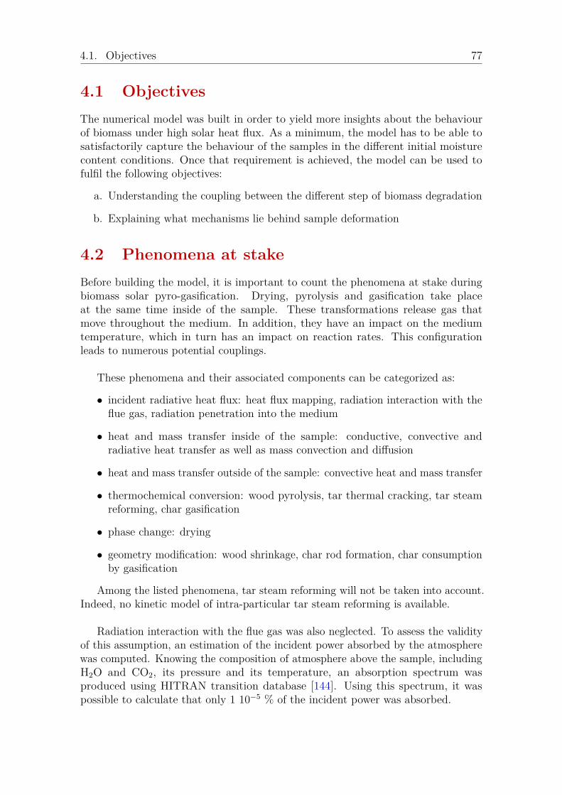
4.1. Objectives 77
4.1 Objectives
The numerical model was built in order to yield more insights about the behaviourof biomass under high solar heat flux. As a minimum, the model has to be able tosatisfactorily capture the behaviour of the samples in the different initial moisturecontent conditions. Once that requirement is achieved, the model can be used tofulfil the following objectives:
a. Understanding the coupling between the different step of biomass degradation
b. Explaining what mechanisms lie behind sample deformation
4.2 Phenomena at stake
Before building the model, it is important to count the phenomena at stake duringbiomass solar pyro-gasification. Drying, pyrolysis and gasification take placeat the same time inside of the sample. These transformations release gas thatmove throughout the medium. In addition, they have an impact on the mediumtemperature, which in turn has an impact on reaction rates. This configurationleads to numerous potential couplings.
These phenomena and their associated components can be categorized as:
• incident radiative heat flux: heat flux mapping, radiation interaction with theflue gas, radiation penetration into the medium
• heat and mass transfer inside of the sample: conductive, convective andradiative heat transfer as well as mass convection and diffusion
• heat and mass transfer outside of the sample: convective heat and mass transfer
• thermochemical conversion: wood pyrolysis, tar thermal cracking, tar steamreforming, char gasification
• phase change: drying
• geometry modification: wood shrinkage, char rod formation, char consumptionby gasification
Among the listed phenomena, tar steam reforming will not be taken into account.Indeed, no kinetic model of intra-particular tar steam reforming is available.
Radiation interaction with the flue gas was also neglected. To assess the validityof this assumption, an estimation of the incident power absorbed by the atmospherewas computed. Knowing the composition of atmosphere above the sample, includingH2O and CO2, its pressure and its temperature, an absorption spectrum wasproduced using HITRAN transition database [144]. Using this spectrum, it waspossible to calculate that only 1 10−5 % of the incident power was absorbed.

78 Chapter 4. Numerical model
Wood shrinkage resulting from drying or pyrolysis was not taken into account.Shrinkage induced by drying was neglected because it is thought that once dried,wood quickly undergoes pyrolysis, therefore limiting the amount of shrunk driedwood. Furthermore, wood shrinkage induced by drying is known to be anisotropicand of little magnitude [37]. It can reach up to 10 % on the tangential directionwhile remaining close to 0 on the longitudinal one [145]. Shrinkage induced bypyrolysis was not taken into account strictly speaking, yet its main consequence, i.e.char rods formation, was described using an homogeneous approach as described inSection 4.7.2.
4.3 Dimensionless numbers and assumptions
In order to get a first insight about the problems at hand, dimensionless numberswere calculated using characteristic values. They should be of help in determiningthe general behaviour of the sample. Then, they are used as guides to chose relevantassumptions during the model construction stage.
4.3.1 Dimensionless numbers
First, a radiative Biot number was calculated for wood (Eq. 4.1) using characteristicvalues of the physical properties available in Table 4.1. As expected, its value isgreater than 1. The sample is therefore not thermally homogeneous.
Bi =φmaxLsp
λwoodδT= 357 (4.1)
Then, Damköhler III numbers were calculated for pyrolysis and gasification(Eq. 4.2 and 4.3). Both of them are greater than 1. Combined with the fact thatBiot number is greater than 1, one can expect the presence of chemical fronts inducedby thermal inhomogeneity for both pyrolysis and gasification.
DaIII, pyro =φ
kpyroρwood∆hpyroLsp
= 75 (4.2)
DaIII, gasi =φ
kgasiρchar∆hgasiLsp
= 116 (4.3)
In addition, pore Reynolds number was calculated (Eq. 4.4). It is around 1,when evaluated in the most unfavourable case. Darcy’s law can therefore be used toderive gas phase velocity with no need for inertial correction [97, 98].
Repore =ρg‖ug‖dpore
µg
= 1.2 (4.4)

4.3. Dimensionless numbers and assumptions 79
Symbol Property Value Dimension
cpg gas phase heat capacity 1004 J/kg/K
dbenzene benzene molecule diameter [146] 5.27 Adpore pore diameter 55.3 µmkB Boltzmann constant 1.380 10−23 J/K
kgasi gasification reaction rate at 800 °C 2.0 10−4 1/skpyro pyrolysis reaction rate at 400 °C 6.2 10−3 1/sLsp sample characteristic length 0.05 mp pressure 101325 Pa
‖ug‖gas phase Darcy’s velocity magnitude(computed as ‖ug‖ = κchar
µg
∆pLsp
) 0.33 m/s
∆hgasi gasification reaction heat 1093.5 kJ/kg∆hpyro pyrolysis reaction heat 80 kJ/kg
∆p maximal internal overpressure [101] 30000 PaδT characteristic temperature difference 1500 Kζ porosity 0.61 -
κchar char permeability [48] 1.0 10−11 m2
λg gas phase thermal conductivity 0.026 W/m/Kλwood sample thermal conductivity 0.1 W/m/K
µg gas phase viscosity 1.8 10−5 Pa.sρchar char density 85 kg/m3
ρg gas phase density 1.2 kg/m3
ρwood wood density 579 kg/m3
φmax max incident heat flux 1072 kW/m2
Table 4.1: Physical properties used for dimensionless numbers calculations

80 Chapter 4. Numerical model
Pore thermal Péclet number was also calculated (Eq. 4.5). Its value is below 1.This has two main consequences: dispersive regime can be ignored [147] andlocal thermal equilibrium can be considered as achieved in the medium [99, 148].Therefore, a single temperature field can be used to describe both solid and gasphase temperatures.
Pepore =ζρgcpg‖ug‖dpore
λg
= 0.52 (4.5)
Finally, Knudsen number was calculated for different conditions: wood at roomtemperature and char at 2000 K. The maximum value is far below 0.01 (Eq. 4.6). Itis therefore possible to use continuum mechanics laws to describe the problem andneglected Knudsen diffusion.
Kn =kBT√
2πd2benzenepdpore
= 4.0 10−3 (4.6)
Based on the different dimensionless numbers values, a schematic diagram ofthe sample during its degradation can be drawn (Fig. 4.1). Drying, pyrolysis andgasification take place at different depths inside of the sample. The gases theyproduce escape the porous medium though a high temperature char layer and aredriven away by the nitrogen sweep.
4.3.2 Assumptions
Assumptions were drawn in order to build the numerical model. Most of them areclassical assumptions used to model transport in porous medium; others are morespecific to biomass degradation:
• wood and char are considered as anisotropic homogeneous porous media
• as discussed before, bois de bout samples are modelled using a 2D axisymmetri-cal geometry. It is made possible because wood and char radial and tangentialphysical properties values are close
• Darcy’s law is used to derive gas phase velocity. This assumption is backed upby pore Reynolds number value
• a single temperature is used to describe solid and gas phase temperatures. Thissimplification is supported by pore thermal Péclet number value
• dispersive regimes are ignored, which is defended by pore thermal Péclet numbervalue
• gases are assumed as ideal
• drying is described using a liquid-vapour equilibrium model
• pyrolysis is described using a pseudo-species model

4.3. Dimensionless numbers and assumptions 81
Figure 4.1: Schematic view of the sample during its degradation
• nine different species are considered: wood, gas, tar, refractory tar, intermediatesolid, char, water, steam and air
• ash is not considered
• model molecules are used to set the physical properties of the different gaseousspecies: benzene is used as model molecule for tar, carbon monoxide for gasand nitrogen for air
• reaction heats are assumed to be constant even though temperature increases
• wood and char are assumed to be gray and diffuse materials, meaning thattheir emissivities equals their absorptivities

82 Chapter 4. Numerical model
4.4 Numerical model
The numerical model aims at describing bois de bout samples under high solar heatflux. As stated before, these samples can be modelled as a 2D axsymmetrical domaininto which conservation equations are solved.
4.4.1 Computational domain
The sample cylinder shape was reduced to wedge under the assumption that it canbe modelled as 2D axsymmetrical (Fig. 4.2). Only bois de bout samples can bemodelled using this method. Furthermore, it is only possible because a special carewas taken in ensuring that the samples fibers were parallel to the incident heat flux.Nevertheless, some limitations to this approach exist; for instance, the nitrogen sweep-ing has a straight direction which is not compatible with 2D axsymmetrical modelling.
The sample is exposed to the incident heat flux on its top boundary. Thetop boundary also allows the gas phase to escape the medium. Side and bottomboundaries are adiabatic gas outlets.
P = 101325 Pa−λeff .∇T.n = −(1− ζ)(1− ξ)αsφ(r, z)
−Ψ(αs, ǫs, r, z, T4, T 4
sur)− h(Tsur − T )∇YI .n = 0
P = 101325 Pa∇T.n = 0∇YI .n = 0
P (r, z, t = 0) = 101325 PaT (r, z, t = 0) = 293 KYI(r, z, t = 0) = YI, ini
ρJ(r, z, t = 0) = ρJ, ini
z
r
Figure 4.2: Computational domain, initial and boundary conditions
The mesh is made of regular prismal and tetrahedral cells. A mesh convergencestudy was led. It demonstrated that 4440 cells is the optimum.

4.4. Numerical model 83
4.4.2 Governing equations
The model is built around the three main equations: mass, momentum and heatconservations.
4.4.2.1 Mass balance
Solid species are immobile. They are governed by classical balance equations(Eq. 4.7):
∂ρJ
∂t=
O∑
K=1
νJ,KωK (4.7)
Gaseous species move through convection and diffusion. They are governed byclassical convection-diffusion equations (Eq. 4.8):
∂ζρgYI
∂t+∇.(ρgugYI) = −∇.(−ρgDs × qg∇YI) +
O∑
K=1
νI,KωK (4.8)
The sample boundaries considered as purely convective outlets (Eq. 4.9).
∇YI .n = 0 (4.9)
Initial wood and water densities are set as measured in Section 2.2.2. One shouldnote that for convenience reasons, Ysteam, ini is calculated by the model. Speciesinitial values are summed up in Table 4.2.
ρJ(r, z, t = 0) = ρJ, ini (4.10)
YI(r, z, t = 0) = YI, ini (4.11)
Species Initial density (kg/m3) Initial mass fraction
Wood Variable (Table 2.3) -Water Variable (Table 2.3) -
Intermediate solid 0 -Char 0 -Gas - 0Tar - 0
Refractory tar - 0Steam - Model calculated
Air - 1 – Ysteam, ini
Table 4.2: Solid, liquid and gaseous phases initial conditions

84 Chapter 4. Numerical model
4.4.2.2 Momentum balance
Gas flow through the sample is described using continuity (Eq. 4.12) combined withideal gas assumption and Darcy’s law.
∂ζρg
∂t+∇.(ρgug) =
O∑
K=1
ωK (4.12)
The gas is assumed to behave as an ideal gas, thus its density can be expressedas:
ρg =pMg
ℜT(4.13)
Combining Eq. 4.12 and 4.13, we obtain Eq. 4.14:
∂
∂t
ζMg
ℜTp +∇.(ρgug) =
O∑
K=1
ωK (4.14)
ug = −κg × qg
µg
(∇p− ρgg) (4.15)
Then, combining Eq. 4.14 and 4.15, we obtain Eq. 4.16:
∂
∂t
ζMg
ℜTp−∇.(ρg
κg × qg
µg
(∇p− ρgg)) =O∑
K=1
ωK (4.16)
The sample boundaries are considered to be outlets at atmospheric pressure(Eq. 4.17).
p = 101325 Pa (4.17)
Initially, the pressure inside of the sample is equal to the atmospheric pressure(Eq. 4.18).
p(r, z, t = 0) = 101325 Pa (4.18)
4.4.2.3 Heat balance
Temperature inside of the medium is governed by Eq. 4.19. It takes into account:heat convection, conduction, radiation with a special formulation of λeff , heatsources and sinks associated with the medium transformation, radiation penetrationinto the medium as a source term (Qpen, see Section 4.7.2) and heat transported bymass diffusive flux.

4.4. Numerical model 85
∂(cpsρs + ζcpgρg + cplw(ρlw + ρbw))T
∂t+∇.(cplw
ρlwulwT ) +∇.(cpgρgugT ) =
−∇.(−λeff∇T ) +O∑
K=1
ωK∆hK −N∑
I=1
∇.(−cpgTρgDs × qg∇YI)
−∇.(−cplwTDbw∇ρbw) + Qpen
(4.19)
Properly predicting temperature is important because it has an impact onbiomass degradation rate and thus on the global behaviour of the model. Therefore,a special care was taken in selecting the medium thermal conductivity model. A widevariety of models exist, ranging from simple classical weighed average estimation[149] to complex consideration on wood pore structure [150]. It was chosen torely on the most advanced model (Eq. 4.20 [143]), which is a modified version ofSaastamoinen and Richard model, in order to include high temperature char thermalconductivity measurements.
λeff =
(1− ζ2/3) λs
1.9+ ζ2/3
1−ζ1/3
2λs1.9
+ ζ1/3
λg
0
0 (1− ζ2/3)λs + ζ2/3
1−ζ1/3
2λs+ ζ1/3
λg
(4.20)
The temperature top boundary condition accounts for radiative heating, aswell as radiative and convective losses (Eq. 4.21). Coefficients multiplying theincident heat flux account for radiation absorption and penetration into the medium(see Section 4.7). Ψ(r, z, T 4, T 4
sur) account for radiative losses. Yet, Ψ is a functiontaking into account the top surface shape. Indeed, when a the crater forms, the cellsinside of the crater to do not have the same view factor toward the surrounding.They also emit and receive energy from the crater inner surface. In order to take thisphenomenon into account, the crater internal view factor are computed assuming ithas a cone shape [151]. The convective heat loss coefficient was chosen as h = 7.0W/m2/K according to the correlation for average heat transfer coefficient over flatplate for a laminar flow provided in [152].
−λeff .∇T.n = −(1−ζ)(1−ξ)αsφ(r, z)−Ψ(αs, ǫs, r, z, T 4, T 4sur)−h(Tsur−T ) (4.21)
Side and bottom boundaries are considered to be adiabatic (Eq. 4.22).
∇T.n = 0 (4.22)
Initially, the temperature is the ambient temperature throughout the sample(Eq. 4.23).
T (r, z, t = 0) = 20 °C (4.23)

86 Chapter 4. Numerical model
4.4.3 Drying model
During a run, water vaporises and moves through the sample. Some of the producedsteam travels to a colder area where it could condense. It was thought that thermalmodels and Arrhenius type models would be too simplistic to accurately describethese phenomena. Drying was therefore modelled using liquid-vapour equilibriumfeaturing liquid, bound water and steam transport. This model is extensivelydescribed in [89]. Only its main features will be described here.
The liquid-vapour equilibrium was described using Eq. 4.24:
psat(T (K)) = exp(7.3649 101 +−7.2582 103
T− 7.3037 log(T ) + 4.1653 10−6T 2) Pa
(4.24)Water motion throughout the sample can be divided into bound water diffusion
(according to the diffusion coefficient Dbw) and liquid water convection under liquidpressure gradient (Eq. 4.25, with δpcap the capillary pressure drop).
ulw = −κlw × qlw
µlw
(∇(p− δpcap)− ρlwg) (4.25)
Where q represents the relative permeability tensors (Eq. 4.26 and 4.27). qg andqlw take into account the fact that when a pore is full of water (S = 1), the gaspermeability tends toward 0.
qg =
(
1 + (2S − 3)S2 00 1 + (4S − 5)S4
)
(4.26)
qlw =
(
S3 00 S8
)
(4.27)
4.4.4 Biomass degradation scheme
Four alternative models are available to describe beech wood degradation: pseudo-species models, cellulose, hemicellulose and lignin models, Ranzi model and FG-DVCmodels. Among them, the two last options seemed over qualified for the task athand. Indeed, given the uncertainty associated with medium physical properties,the quality of their predictions would be hindered by slight misprediction of thetemperature field and species transport. Between, the two first options, it was chosento resort on comparison led in literature [104] which advised a pseudo-species model.
Pyrolysis is described using a pseudo-species model which is the combinationof existing models (Fig. 4.3). One should note that even if the degradation modelcomponents were chosen with care, it was not possible to find in literature kineticparameters derived for our conditions, i.e. 250 K/min heating rate and highfinal temperature. The closest available kinetic parameters were therefore chosen

4.4. Numerical model 87
[55, 63, 103, 104]. These parameters been validated against 50 to 100 K/min heatingrates experiments, with a pyrolysis final temperature around 600 °C. Furthermore,this model does not predict gas nor tar compositions.
The specificity of the chosen model is the use of an intermediate solid pseudo-specie to mimic lignin. Indeed, lignin is the main precursor of char and its degradationis known to be exothermic. Intermediate solid behaviour is set accordingly, i.e. itdegrades into char releasing heat.
Water Steam
Gas
Wood Tar
Refractory tar
Intermediate solid Char
k2
k3
k4
k5
k7
k6
k8
k9
k1
Figure 4.3: Biomass drying model and pyrolysis scheme
Number Reaction A (1/s) Ea (kJ/mol) ∆h (kJ/kg) Reference
1 Wood 7→ steam 4.38 109 × a 152.7 -80 [63, 104]2 Wood 7→ gas 4.38 109 152.7 -80 [104]3 Wood 7→ tar 1.08 1010 × (1-a) 148.0 -80 [63, 104]4 Wood 7→ intermediate solid 3.75 106 × b 111.7 -80 [104]5 Tar 7→ gas 2.15 1011 141.0 42 [103]6 Tar 7→ char 1.0 105 108.0 42 [103]7 Tar 7→ refractory tar 1.16 1011 141.0 42 [103]8 Intermediate solid 7→ char 1.38 1010 161.0 300 [104]
Table 4.3: Kinetic parameter for beech wood pyrolysis. a = 0.219 [63] and b = 2
Reaction rates follow first order kinetics. They are therefore obtained by multi-plying reaction rate coefficients (Eq. 4.28) by reagent density and νI,J coefficients,according to Eq. 4.29 for gases reagents and to Eq. 4.30 for solid reagents. νI,J,K
are stoichiometric coefficients taking the value of 0 or 1 according to the degradationscheme (Fig. 4.3).
kK = AK exp(EaK
ℜT) (4.28)
ωK = kKρg
N∏
I=1
νI,KζYI (4.29)

88 Chapter 4. Numerical model
ωK = kK
M∏
J=1
νJ,KρJ (4.30)
Gasification reaction rate features both char density and steam mass fractiondependency (Eq. 4.31). It was established for the steam gasification of char obtainedfrom flash beech wood pyrolysis [113].
ωgasi = ω9 = 4.20 104 exp(150750
ℜT)ρ0.58
charζYsteam (4.31)
Modifications were applied to the kinetic schemes found in literature. The firstone is the introduction of water production in the pyrolysis scheme. According to[63], 21.9 % of the tar produced by beech wood flash pyrolysis is in fact water. Arepartition factor, called a, was therefore applied to derive pyrolysis water production.
In order to get credible results, it was mandatory to modify pyrolysis schemechar production. Indeed, the initially produced amount of char was extremely lowand led to a 98 % porosity char, which is not credible. One should keep in mind thatthe used kinetic scheme has not been tested for high pyrolysis final temperature.The char production kinetic parameter was corrected by a factor called b, taken as 2.Given the intrinsic weakness that is the dependency on these kinetic schemes, it waschosen to keep the correction factor with only one significant digit. This correctionyields char with 95 % porosity, which is in agreement with the literature dealingwith high temperature pyrolysis [42].
4.5 Physical properties
In order to accurately model the solar pyro-gasification of wood, it is key to knowits physical properties. As stated before, there is a wide range of variability hiddenbehind the name wood. Physical properties can vary by one order of magnitude fromspecies to species [18].
The model developed in this work is based on heat, momentum and massbalances. Therefore, the physical properties of interest are : porosity, density,thermal conductivity, specific heat capacity, radiation absorptivity, permeability andmass diffusivity. As for other porous media, porosity is the central physical propertybecause is has an impact on every other physical properties at the Darcy’s scale.
Finally, one should keep in mind that wood is an anisotropic material. Heat andmass transfers are favoured in the fiber direction. Yet, the apparition of cracks inthe structure can locally modify heat and mass transfer patterns [153].

4.5. Physical properties 89
4.5.1 Solid phases
4.5.1.1 Wood
Dry wood porosity ranges from 40 to 60% [121]. Regarding beech wood, the poremean diameter is 55.3 ± 11.7 µm [154] while the largest pores have a diameter of500 µm [34].
Because of its anisotropy, measuring wood thermal conductivity is a challengingtask that was undertaken by several authors. Thermal conductivity is deduced fromheat diffusion coefficient and specific heat capacity measurements [155]. Authorshave gathered measurements over a wide range of wood species and conditions suchas temperature or moisture [32]. Some of them make an explicit difference betweenthe directions, others not. As a general rule, one can state that wood thermalconductivity is around 0.1 W/m/K in the fiber direction. This value can be dividedby 2 in the two other directions.
Wood radiation absorptivity is usually considered to be high. Measurements inboth IR and visible ranges show a wide spectral variation of the absorptivity. In theIR range, absorptivity was reported to vary between 0.80 and 0.90 depending on theradiation source temperature [82, 156]. While is was reported to be close to 0.50in the visible range [157]. It was therefore chosen to rely on the values that werecalculated based on our measurements (Section 2.2.2). Wood absorptivity was alsoexamined with respect to wood thermal breakdown level. It was shown to flattendramatically by increasing in the visible range while slightly decreasing in the IR [157].
The chosen values of beech wood the physical properties are available in Table4.4. The properties that could not be measured were taken from literature. When achoice had to be made between two correlations, the one with the wider validityrange was preferred. A summary of a wood physical properties literature survey canbe found in Tables B.1 and B.2 in Appendix B.
4.5.1.2 Char
Char is a porous material. Its porosity is therefore a key parameter that controlsevery physical property of this material. However, char porosity is known to varywith pyrolysis conditions, i.e. heating rate and final temperature. For instance, forthe same final temperature, a porosity of 88 was reported % with a heating rate of900 K/min while it was 73 % for a heating rate of 2.6 K/min [47]. Furthermore,during gasification char porosity increases until char is fully consumed.
Classically, reported value of char thermal conductivity are about 0.1 W/m/Kat room temperature. It is important to note that because char is a very porousmaterial, radiative heat transfer occurs inside of it and thus increases its effectivethermal conductivity. For an insulating material similar to char, a multiplication by6 of the thermal conductivity between 20 and 1127 °C was reported [159]. There is

90 Chapter 4. Numerical model
a wide variety of models taking this contribution into account ranging from basicRossland [160] and to more complex models [150, 161]. To this date, only one studyreports measurement of char thermal conductivity at high temperature (900 °C)[143]; others are limited to 300 °C.
Char physical properties are also modified by its geometry at a higher level thanthe pore scale. At the macroscopic scale, both high heating rate and gasificationcan induce cracks [14, 47]. These cracks have an impact on local thermal andhydrodynamic properties, yet no work could be found on that subject.
Char emissivity is considered to be close to 1 because of its dark color and thenumerous cavities it exhibits on its surface. Nevertheless, only two measurements forbeech could be found in literature: 0.94 in [162] and 0.88 [109]. These values arecoherent with an in depth study led on plywood [163].
The chosen values of char physical properties are available in Table 4.5. Exceptabsorptivity, all the values come from literature. A summary of a char physicalproperties literature survey can be found in Tables B.3 and B.4 in Appendix B.Some needed physical properties of char are not readily available in literature; theyhave therefore been estimated.
Char porosity being unknown and varying thoughout the medium, is calculatedusing char intrinsic density taken as ρchar, intrinsic = 1700 kg/m3 [49] according toEq. 4.32.
ζchar = 1− ρchar
ρchar, intrinsic
(4.32)
Only longitudinal values were available for char permeability [48]. It was chosento keep wood permeability anisotropic ratio to build char permeability tensor (Eq.4.33).
κchar = 1 10−11
(
99.7 10−6 00 1
)
(4.33)
Char mass diffusion coefficient was not available in literature. It was chosen tokeep wood diffusivity tensor and correct it by char/wood porosity ratio (Eq. 4.34).
Dchar =ζchar
ζwood
Dwood (4.34)
4.5.1.3 Solid phase properties evaluation
Solid phase properties are calculated as the weighed average of wood and charproperties (Eq. 4.35). Intermediate solid phase is considered as char when calculatingthe physical properties.

4.6. Moving mesh strategy 91
κs =ρwoodκwood + (ρis + ρchar)κchar
ρwood + ρis + ρchar
(4.35)
Ds is the mass diffusion coefficient. Being directly measured in wood [34],it does not need to be multiplied by the classical ζ/τ correction that is used toevaluate the diffusion coefficient in porous medium based on gas diffusivity. Massdiffusion coefficient are known to evolve with temperature [164]. Unfortunately,no law governing the evolution of this coefficient was found in literature. It wastherefore chosen to affect a classical temperature dependency for diffusion coefficient(Eq. 4.36 [165]).
Ds(T (K)) = Ds|293 K(T
293)1.5 (4.36)
4.5.2 Gas phase
Gas phase properties are calculated as the weighed average of every single gaseousspecies properties (Eq. 4.37). Individual gas phase properties are available inAppendix C.
cpg =N∑
I=1
cpIYI (4.37)
In order to take into account the fact that the pore can be full of water (S = 1),a special equation is used for gas phase thermal conductivity (Eq. 4.38).
λg = Sλlw + (1− S)N∑
I=1
λIYI (4.38)
4.6 Moving mesh strategy
As experimentally observed, steam gasification consumes the char produced bypyrolysis, leading to a disappearance of the medium. In terms of numerical modelling,this translates into the fact that solid phase density can reach 0 kg/m3 at the topboundary cells. In order to correctly take this phenomenon into account, a solidmedium deformation strategy has to be implemented.
Phase field method has successfully been used in literature for a similar case[115]. This kind of method assigns a field to the solid medium, generally varyingbetween 0 and 1. This field can move on a fixed mesh, describing the solid mediumshape evolution. Yet, it did not seem adapted to radiative heat transfer in the wayit is described in this model. Indeed, in order to properly take into account theradiative heating contribution, penalized cells with very high thermal conductivitywould be required in order to transfer radiative heat to the solid medium boundaryas fast as possible.
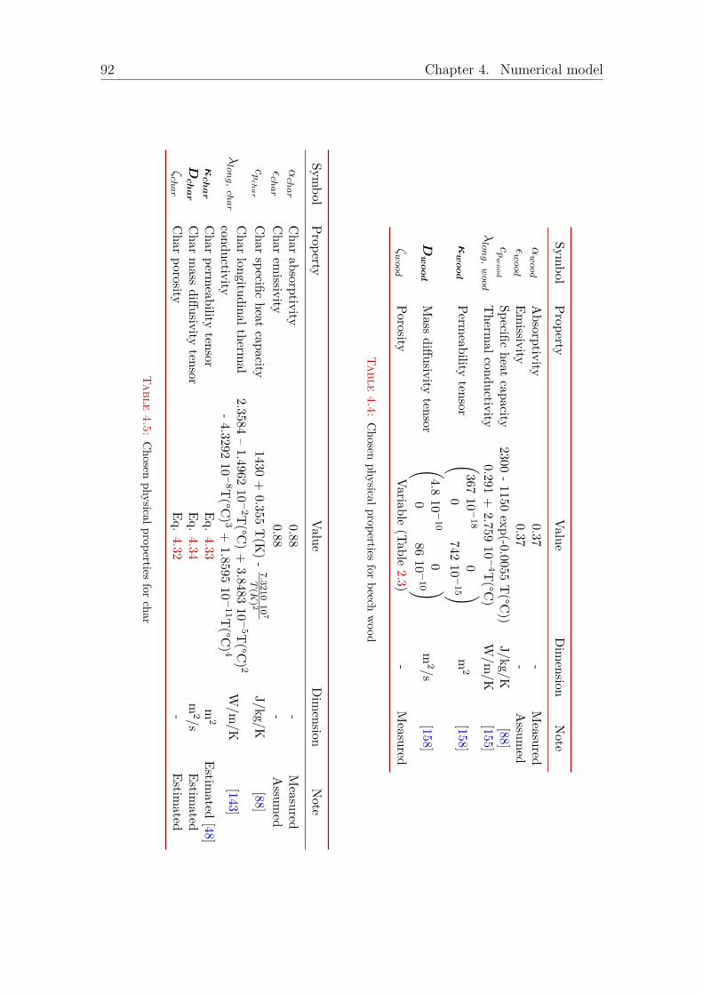
92 Chapter 4. Numerical model
Sym
bol
Prop
ertyV
alue
Dim
ensio
nN
ote
αw
ood
Absorp
tivity
0.37-
Measu
redǫw
ood
Em
issivity
0.37-
Assu
med
cp
wo
od
Sp
ecific
heat
capacity
2300-
1150ex
p(-0.0055
T(°C
))J/k
g/K
[88]λ
lon
g,
wood
Therm
alcon
ductiv
ity0.291
+2.759
10−
4T(°C
)W
/m/K
[155]
κw
oo
dP
ermeab
ilityten
sor
(
36710
−18
00
74210
−15
)
m2
[158
]
Dw
oo
dM
assdiff
usiv
ityten
sor
(
4.810
−10
00
8610
−10
)
m2/s
[ 158]
ζw
ood
Porosity
Variab
le(T
able
2.3)-
Measu
red
Ta
ble
4.4:C
hosen
physical
prop
ertiesfor
beech
wood
Sym
bol
Prop
ertyV
alue
Dim
ension
Note
αch
ar
Char
absorp
tivity
0.88-
Mea
sured
ǫch
ar
Char
emissiv
ity0.88
-A
ssum
ed
cp
ch
ar
Char
specifi
cheat
capacity
1430+
0.355T
(K)
-7.3
210
10
7
T(K
)2
J/k
g/K
[ 88]
λlo
ng,
cha
rC
har
longitu
din
alth
ermal
2.3584–
1.496210
−2T
(°C)
+3.8483
10−
5T(°C
)2
W/m
/K
[ 143]
conductiv
ity-
4.329210
−8T
(°C)3
+1.8595
10−
11T
(°C)4
κch
ar
Char
perm
eability
tensor
Eq.
4.33m
2E
stimated
[48]
Dch
ar
Char
mass
diff
usiv
ityten
sorE
q.
4.34m
2/sE
stimated
ζch
ar
Char
porosity
Eq.
4.32-
Estim
ated
Ta
ble
4.5:C
hosen
physical
prop
ertiesfor
char

4.6. Moving mesh strategy 93
Arbitrary Lagrangian Eulerian technique [117] allows to deform a mesh andcan therefore be a solution to property take into account the radiative boundarycondition. With this technique, the velocity is affected to mesh cells and solved fieldsare corrected to prevent the mesh velocity from inducing errors. This approach wassuccessfully used to model space shuttle ablative thermal shield behaviour [116]. Yet,it requires an heavy reformulation of the model equations and the determination ofa mesh velocity properly describing solid phase geometry evolution.
A third way was chosen: mesh interpolation, for it does not require governing equa-tions reformulation nor mesh velocity determination. With this technique an ablationcriterion is set, in our case when char porosity exceeds 0.975 (or ρchar < 42.5 kg/m3,Fig. 4.4, A). When a cell satisfies this criterion, the mesh evolves in such a way thatit simulates solid phase ablation (Fig. 4.4, B and C).
Once the mesh has been updated, the solved fields need to be recalculated so thatthey would reflect char ablation. First, the cells overlapping volumes between theformer and the current mesh are computed. Then, the solved fields are interpolatedbased on the overlapping volumes (Fig. 4.4, D). In order to ensure that mass andenergy are conserved, the special treatment has to be applied to the top row cells.The solid mass and energy remaining in the ablated cell is added to the cell below,therefore, no mass nor energy disappears. The same is done with the two cells thatneighbours the ablated cell. Indeed, in the process of moving the ablated cell, halfof their volumes disappears. It is taken into account to prevent mass or energydisappearance. Finally, when interpolating the solved fields, gaseous species are leftfree to escape the medium.
Once the mesh has been updated and the solved fields interpolated, the simulationcarries on using the modified geometry (Fig. 4.4, E).
This technique is quite easy to understand and allows for great flexibility. Yet, ithas one main drawback: it is heavy to implement (or even impossible to implementin closed-source solvers). Implementing this technique required to use a numericalsolver allowing for a great level of freedom in terms of source code modifying. Thisis why the open source OpenFOAM CFD framework was chosen to implement themodel.

94 Chapter 4. Numerical model
ρchar > ρchar, lim
ρchar > ρchar, lim
ρchar > ρchar, lim
ρchar > ρchar, lim
ρchar > ρchar, lim
ρchar > ρchar, lim
ρchar > ρchar, lim
ρchar > ρchar, lim
ρchar > ρchar, lim
(a) No cell satisfies the ablation criterion
ρchar > ρchar, lim
ρchar > ρchar, lim
ρchar > ρchar, lim
ρchar > ρchar, lim
ρchar > ρchar, lim
ρchar > ρchar, lim
ρchar > ρchar, lim
ρchar > ρchar, lim
ρchar > ρchar, limρchar < ρchar, lim
(b) Gray cell satisfies the ablation criterion
ρchar = ρ1 ρchar = ρ2 ρchar = ρ3
ρchar = ρ4 ρchar = ρ5 ρchar = ρ6
ρchar = ρ7 ρchar = ρ8 ρchar = ρ9
(c) Fields before mesh motion are stored for futurerecalculation
ρchar = ρ′1
ρchar = ρ10
ρchar = ρ′3
ρchar = ρ′4
ρchar = ρ′5
ρchar = ρ′6
ρchar = ρ′7
ρchar = ρ8
ρchar = ρ′9
+δV1ρ1
+V2ρ2
+δV3ρ3
δV1
ρ1
V2
ρ2
δV3
ρ3
(d) Mesh is moved and fields are interpolated
ρchar > ρchar, lim
ρchar > ρchar, lim
ρchar > ρchar, lim
ρchar > ρchar, lim
ρchar > ρchar, lim
ρchar > ρchar, lim
ρchar > ρchar, lim
ρchar > ρchar, lim
ρchar > ρchar, lim
(e) No cell satisfies the ablation criterion, the simula-tion carries on
Figure 4.4: Mesh motion technique

4.7. Radiation penetration strategies 95
4.7 Radiation penetration strategies
Radiation penetrates the medium at two levels: close to the surface, inside of woodand char porosity (referred as near surface penetration); in between char rods directlyto the bottom of the crater (referred as in depth penetration). The radiative powerthat penetrates the medium is taken into account as a source term: Qpen.
4.7.1 Near surface penetration
The incident radiation penetrates the medium thought wood and char porosity.Indeed, beech wood pores mean diameter (55.3 µm [154]) is much greater than theincident radiation wavelength: radiation behaves ballistically in the medium porousgeometry.
Radiation penetration length was estimated to be around 52 µm into wood and66 µm into char (Appendix D). Near surface penetration has been implementedinto model. If the penetration depth is larger than the cell height, the penetratingincident power is uniformly distributed over the cells until the penetration depth isreached.
4.7.2 In depth penetration
The incident radiation also penetrates the medium in between char rods. Deformingthe mesh in order to describe each and every rod was not accessible. Therefore,an homogeneous approach was chosen. The crater is considered to be char and isdescribed using char physical properties. A volume field (Qpen) is built in order totake into account, in the heat balance equation, the radiative power which penetratesinto the sample. This field is constructed considering that a fraction (ξ) of theincident power reaching the top boundary of the sample propagates ballisticallythrough the char crater. The remaining fraction (1 − ξ) of the incident radiativepower is distributed between the top boundary and the char upper surface porosityfollowing the near surface penetration model (see Section 4.7.1). The in depthpenetrating power propagates into the medium until it reaches the pyrolysis front,defined as the first cell where ρwood > ρis + ρchar. Half of it is uniformly absorbed onits way to the bottom of the crater. The remaining half is absorbed once it reachesthe pyrolysis front. There, it is distributed following the radiation near surfacepenetration model. Then, the Qpen field is built by dividing, in every cell, the localamount of penetrating power by the cell volume. Once built, the Qpen field is treatedas a source term in the heat balance equation (Eq. 4.19).
Four different approaches were tested in order to model in depth radiationpenetration. These approaches are detailed in Figure 4.5. Then their results arecompared to experimental observations (Fig. 3.9). For the sake of simplicity, meshmotion was deactivated while producing illustrating results (Fig. 4.6). 0 %wb initial

96 Chapter 4. Numerical model
(a) No in depth radiation penetration (b) Collimated in depth radiation penetra-tion
(c) Collimated in depth radiation penetra-tion with internal emission
(d) Uncollimated in depth radiation penetra-tion
Figure 4.5: Radiation penetration strategies. Light gray: wood, dark gray: char
moisture content cases were chosen to illustrate the different penetration strategiesbecause the initial lack for water reduces the error induced by mesh deformationand char gasification deactivation.
At first, no radiation penetration was considered (Fig. 4.5 A), i.e. ξ = 0 andQpen(r, z, t) = 0. As a result, a layer of char appears on the upper part of the sample(Fig. 4.6 A). This layer has a low thermal conductivity and acts as a thermal shield,preventing the pyrolysis of the major part of the sample. This approach fails toreproduce experimentally observed sample behaviour.
Then, radiation is considered to be vertical and collimated. It is allowed topenetrate the medium until it reaches the pyrolysis front (Fig. 4.5 B). The amountof radiation penetrating the medium is determined considering usual wood tochar shrinkage proportion. It is known that char volume is 65 % lower than theinitial wood volume. Thus, for a surface, the contraction would be around 50 %

4.7. Radiation penetration strategies 97
ρchar (kg/m3)
(a) No in depth radiation penetration (b) Collimated in depth radiation pene-tration
(c) Collimated in depth radiation pene-tration with internal emission
(d) Uncollimated in depth radiation pen-etration
Figure 4.6: Radiation penetration strategies results for 0 %wb initial moisture content boisde bout cases after a 5 minutes exposure (mesh deformation and char gasification deactivated).Colormap: char density
(ξ = 0.50). This value was confirmed by image processing method of char craterpicture (Fig. 3.8). The numerical results show a char crater (Fig. 4.6 B). Yet, itsshape and depth do not match experimental observations. The crater is too sharp.
Two mechanisms were envisioned to explain the flattening of the crater. The firstone is internal rod to rod radiation which could greatly enhance radial heat transfer(Fig. 4.5 C). By considering that the gap between the char rods is negligible beforetheir height and by linearising radiative heat transfer, using Rossland model [160],it is possible to associate a thermal conductivity to internal radiation. Then, aneffective radial thermal conductivity is built considering that char and radiativethermal conductivities are in serial configuration. Taking internal radiation intoaccount did change the results by 2 % in terms of crater depth (Fig. 4.6 C). It istherefore thought that it is not the main crater flattening mechanism.
Finally, in the actual configuration, the incident radiation is not collimated. The12.98° aperture angle of the incident beam was taken into account (Fig. 4.5 D).Considering that all the beams cross at the same point and knowing the beamaperture angle and the focal spot radius, it is possible to determine this crossingpoint. This point is used as a homothetic center (H) to project the incident heat fluxon the pyrolysis front (Fig. 4.7). The predicted crater shape is in good agreement

98 Chapter 4. Numerical model
rfs
12.98◦
H
Figure 4.7: Radiation in depth penetration strategy. On the left: homothetic center construction,on the right: incident heat flux projection
with experimental observations (Fig. 4.6 D). It is therefore though that incidentradiation aperture angle is the crater flattening phenomenon.
4.8 Numerical methods
The governing equations were implemented and solved using the open sourceOpenFOAM CFD framework [166, 167]. It was chosen because the accessibilityof its source code allowed for the implementation of moving mesh and radiationpenetration strategies.
OpenFOAM offers a wide variety of numerical schemes for time and spacedifferencing. A second order backward scheme was chosen for time integration.Source terms were solved implicitly when possible.
Linear differencing was used for spatial differencing. Regarding divergencedifferencing, off-centred limited schemes, such as Van Leer or Gamma schemes, weretried. Despite their high computational cost, they did not improve the results quality.
After a solver tolerance convergence study, equations solvers tolerances wereset to 10−12, except for pressure which was set to 10−18. Solving pressure equationis a challenging task in this particular case. Indeed, sharp porosity discontinuity,induced by the pyrolysis front, creates spurious fluxes in the pressure matrix.These fluxes can, in turn, lead to artefacts in the pressure fields (Fig. 4.8). Thisproblem can be solved for a given range of Darcy’s number in the case isotropicporous media, without mass source term [168]. The method mainly consists in

4.8. Numerical methods 99
implicitly solving the flow resistance. Applying this method to our case did notproduce any improvement. According to the creator of the proposed method,it remains a state of the art problem for anisotropic cases with mass sourceterms. Nevertheless, it was checked that, at the sample scale, mass conversationwas not hindered by this problem. Yet, regarding individual mass fractions, 10 %errors may be induced with a sum of the mass fractions varying between 0.90 and 1.10.
p (Pa)
(a) A pressure field without artefact (b) A pressure field with artefacts
Figure 4.8: Two pressure fields in the reference case (9 %wb, bois de bout)
Time step was constrained by a Courant number and a maximum vaporisationrate. The Courant number was the most restrictive criterion. A time step conver-gence study showed that no further improvement could be obtained by loweringthe maximum Courant number below 0.5, which was therefore chosen as maximumCourant number value.
Conclusion
This chapter presented the numerical model used in the modelling part of this work.This model is based on three main conservation equations: mass, momentum andheat balances. These equations are coupled with liquid-vapour equilibrium dryingmodel and pseudo-species biomass degradation model. Assumptions made to writethese equations are defended using dimensionless numbers. Because of biomass solarpyro-gasification specific nature, i.e. medium gasification and radiation penetration,special strategies have been implemented to describe medium shape evolution andincident heat flux penetration into the crater geometry. Finally, it was shown thatbeam spreading is the mechanism that controls the crater shape.


CHAPTER 5Numerical results
Introduction . . . . . . . . . . . . . . . . . . . . . . . . . . . . . . 102
5.1 Assumptions validation . . . . . . . . . . . . . . . . . . . . 102
5.2 Comparison with experimental observations . . . . . . . 103
5.3 General behaviour . . . . . . . . . . . . . . . . . . . . . . . 105
5.3.1 Drying . . . . . . . . . . . . . . . . . . . . . . . . . . . . . 106
5.3.2 Tar production . . . . . . . . . . . . . . . . . . . . . . . . 107
5.3.3 Char steam gasification . . . . . . . . . . . . . . . . . . . 109
5.4 Sensitivity analyses . . . . . . . . . . . . . . . . . . . . . . 110
5.4.1 Sensitivity to the drying model . . . . . . . . . . . . . . . 110
5.4.2 Sensitivity to b fitting parameter . . . . . . . . . . . . . . 113
5.4.3 Sensitivity to the pyrolysis model . . . . . . . . . . . . . . 114
Conclusion . . . . . . . . . . . . . . . . . . . . . . . . . . . . . . . 115
101

102 Chapter 5. Numerical results
Introduction
This chapter presents the results produced by the numerical model. Thetwo first parts assess the validity of the model predictions. Once thevalidity of the model has been established, further insights on biomass solar
pyro-gasification are derived from its predictions. Finally, the robustness of thechoices made for the construction of the model is assessed through sensitivity analyses.
The first part deals with the validation of the assumptions that were made inorder to build the model. Key dimensionless number values are verified to be withinreasonable bounds so that assumptions validity is not hindered.
The second part compares numerical model predictions with experimentalobservations. The numerical model results are analysed qualitatively by comparingnumerical and experimental geometries and quantitatively by confronting predictedand observed temperature and time averaged production/consumption rates.
The third part analyses the predicted behaviour of biomass. Using the model,further insights on biomass behaviour under high solar heat flux are derived andcouplings between different phenomena at stake are highlighted.
The last part reports the results of different sensitivity analyses. Drying andpyrolysis models were modified in order to assess their impact on the model results.Furthermore, the impact of the fitting parameter b on the general behaviour of themodel was analysed using a sensitivity analysis.
5.1 Assumptions validation
In order to assess the model construction assumptions validity, key dimensionlessnumbers were extracted at every time step. Their maximum values were thenconfronted with the critical values that they should not exceed.
The maximum reported value for pore Reynolds number is 0.15. It remains belowthe critical value of 1 and thus validates the choice of the uncorrected Darcy’s lawfor deriving velocity from pressure gradient.
The maximum value taken by the pore Péclet number is 7.1 10−2 which is below1. It validates the use of one temperature field to describe both solid and gas phasetemperatures.
The highest reported value of Knudsen is 3.3 10−3. This value being below0.01; the laws of continuum mechanics could be used without any need for corrections.
In addition, and as a token of the quality of this model, mass and energy

5.2. Comparison with experimental observations 103
conservation were checked at the sample scale. Over a run, mass and energy areconserved at more than 99.9 %.
5.2 Comparison with experimental observations
Before analysing model predictions in depth, numerical results are compared toexperimental observations in order to assess their validity.
ρchar (kg/m3)
Experimental observations Numerical predictions
(a) 0 %wb initial moisture content (b) 0 %wb initial moisture content
(c) 9 %wb initial moisture content (d) 9 %wb initial moisture content
(e) 55 %wb initial moisture content (f) 55 %wb initial moisture content
Figure 5.1: Experimental and numerical crater cut views. Colormap: char density
On a qualitative level, the predicted sample geometries and the char densityfields are compared with the experimental observations for the three different initialmoisture contents (Fig. 5.1). The predicted crater depths and widths are close tothe ones experimentally observed. It is a token of the quality of the solid fields
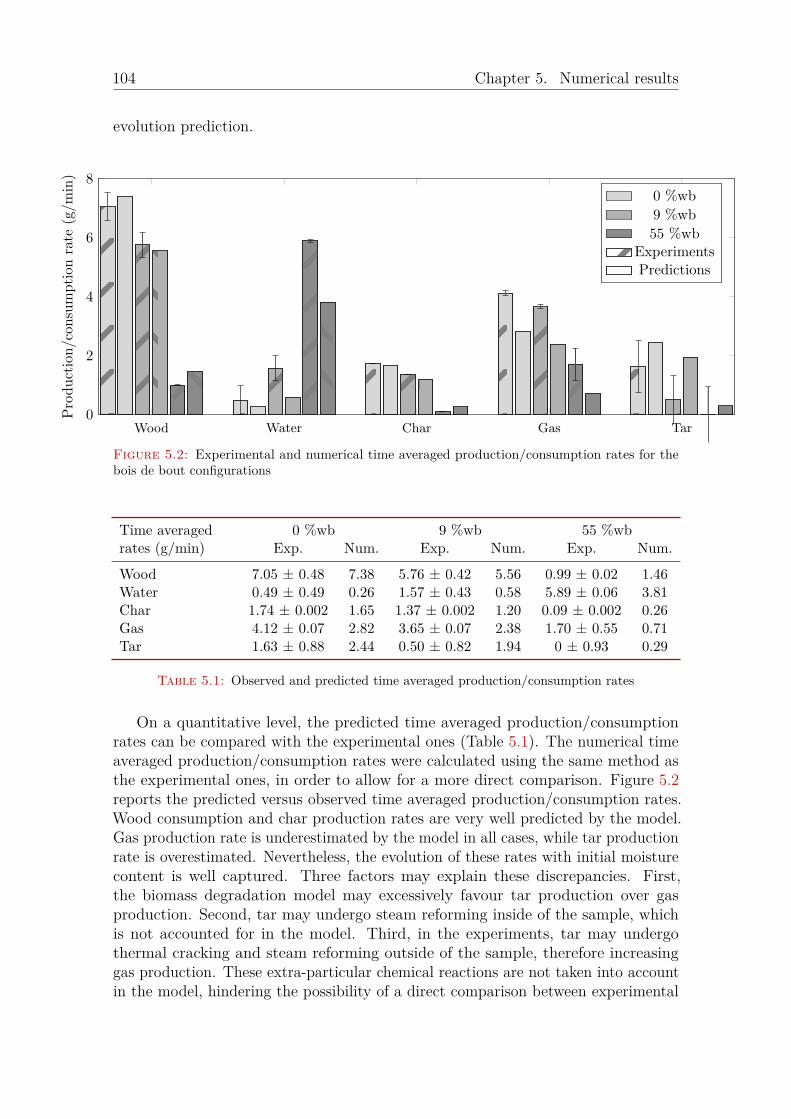
104 Chapter 5. Numerical results
evolution prediction.
Wood Water Char Gas Tar0
2
4
6
8
Production/con
sumption
rate
(g/m
in)
0 %wb
9 %wb
55 %wbExperimentsPredictions
Figure 5.2: Experimental and numerical time averaged production/consumption rates for thebois de bout configurations
Time averagedrates (g/min)
0 %wb 9 %wb 55 %wbExp. Num. Exp. Num. Exp. Num.
Wood 7.05 ± 0.48 7.38 5.76 ± 0.42 5.56 0.99 ± 0.02 1.46Water 0.49 ± 0.49 0.26 1.57 ± 0.43 0.58 5.89 ± 0.06 3.81Char 1.74 ± 0.002 1.65 1.37 ± 0.002 1.20 0.09 ± 0.002 0.26Gas 4.12 ± 0.07 2.82 3.65 ± 0.07 2.38 1.70 ± 0.55 0.71Tar 1.63 ± 0.88 2.44 0.50 ± 0.82 1.94 0 ± 0.93 0.29
Table 5.1: Observed and predicted time averaged production/consumption rates
On a quantitative level, the predicted time averaged production/consumptionrates can be compared with the experimental ones (Table 5.1). The numerical timeaveraged production/consumption rates were calculated using the same method asthe experimental ones, in order to allow for a more direct comparison. Figure 5.2reports the predicted versus observed time averaged production/consumption rates.Wood consumption and char production rates are very well predicted by the model.Gas production rate is underestimated by the model in all cases, while tar productionrate is overestimated. Nevertheless, the evolution of these rates with initial moisturecontent is well captured. Three factors may explain these discrepancies. First,the biomass degradation model may excessively favour tar production over gasproduction. Second, tar may undergo steam reforming inside of the sample, whichis not accounted for in the model. Third, in the experiments, tar may undergothermal cracking and steam reforming outside of the sample, therefore increasinggas production. These extra-particular chemical reactions are not taken into accountin the model, hindering the possibility of a direct comparison between experimental
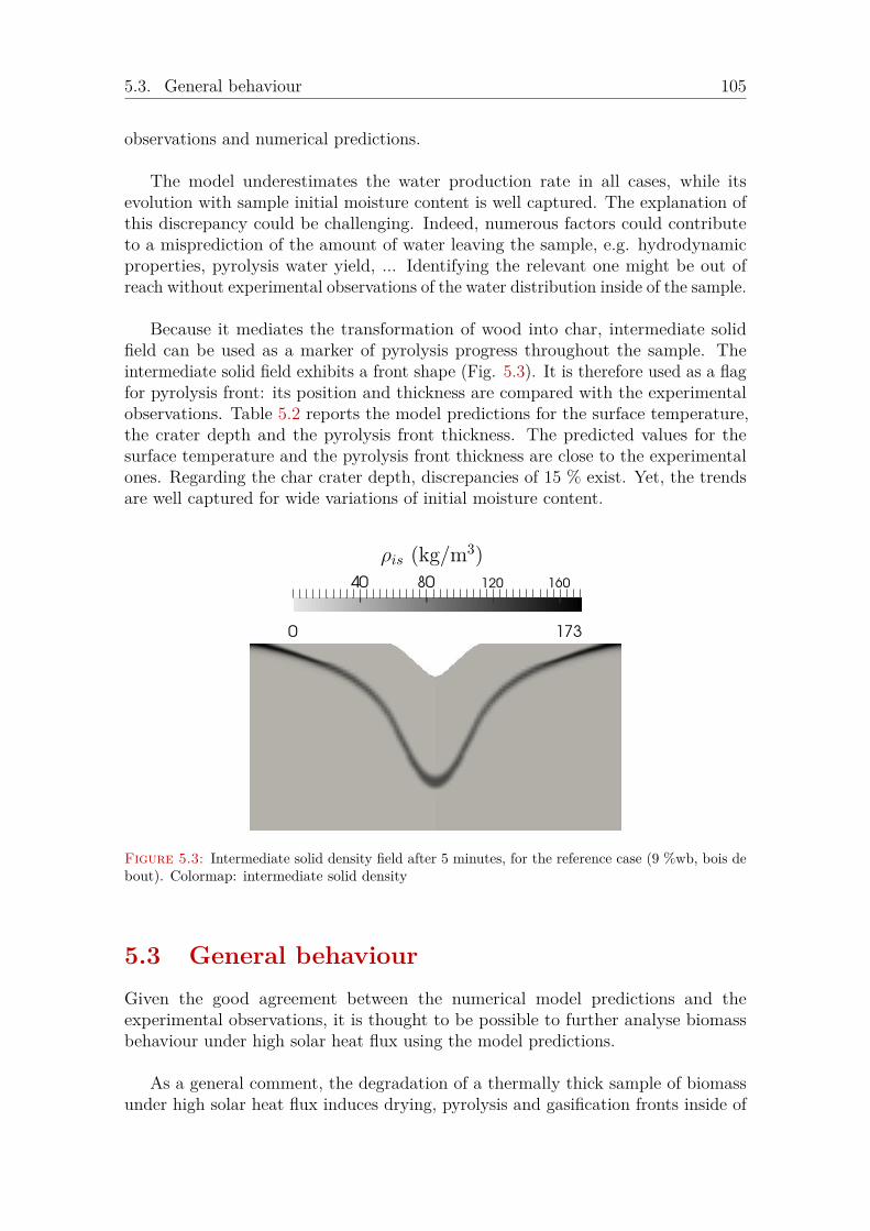
5.3. General behaviour 105
observations and numerical predictions.
The model underestimates the water production rate in all cases, while itsevolution with sample initial moisture content is well captured. The explanation ofthis discrepancy could be challenging. Indeed, numerous factors could contributeto a misprediction of the amount of water leaving the sample, e.g. hydrodynamicproperties, pyrolysis water yield, ... Identifying the relevant one might be out ofreach without experimental observations of the water distribution inside of the sample.
Because it mediates the transformation of wood into char, intermediate solidfield can be used as a marker of pyrolysis progress throughout the sample. Theintermediate solid field exhibits a front shape (Fig. 5.3). It is therefore used as a flagfor pyrolysis front: its position and thickness are compared with the experimentalobservations. Table 5.2 reports the model predictions for the surface temperature,the crater depth and the pyrolysis front thickness. The predicted values for thesurface temperature and the pyrolysis front thickness are close to the experimentalones. Regarding the char crater depth, discrepancies of 15 % exist. Yet, the trendsare well captured for wide variations of initial moisture content.
ρis (kg/m3)
Figure 5.3: Intermediate solid density field after 5 minutes, for the reference case (9 %wb, bois debout). Colormap: intermediate solid density
5.3 General behaviour
Given the good agreement between the numerical model predictions and theexperimental observations, it is thought to be possible to further analyse biomassbehaviour under high solar heat flux using the model predictions.
As a general comment, the degradation of a thermally thick sample of biomassunder high solar heat flux induces drying, pyrolysis and gasification fronts inside of

106 Chapter 5. Numerical results
0 %wb 9 %wb 55 %wbExp. Num. Exp. Num. Exp. Num.
Surface temperature (°C) 1594 ± 123 1515 1530 ± 120 1526 1317 ± 98 1337Crater depth (cm) 4.5 3.9 3.2 3.7 2.4 2.2Pyrolysis front thickness(mm)
4 4 3 4 0.5 0.5
Table 5.2: Observed and predicted surface temperature, crater depth and pyrolysis front finalthickness
the sample. This general behaviour is in good agreement with the dimensionlessnumber predictions. The main part (about 90 %) of the produced gases are forcedtoward the top boundary and therefore go through a high temperature char layerbefore escaping from the medium. This configuration is very likely to lead to physicalcouplings between the phenomena at stake during biomass degradation under highsolar heat flux.
5.3.1 Drying
During a run, a drying front can be observed for the three initial moisture contents.The water density field exhibits the same shape in all cases. The field can be dividedinto three zones (Fig. 5.4 and Fig. 5.5):
• a dry zone (in light gray on Fig. 5.4), where the temperature is far above100 °C
• a condensation zone (in black on Fig. 5.4), in which steam is forced bythe pressure gradient. In this zone, steam condenses. Condensation beingexothermic, steam condenses until the temperature reaches a value close to100 °C and moisture content rises to an equilibrium value of 84 kg/m3
• an unmodified zone (in dark gray on Fig. 5.4), where the moisture is equal tothe initial moisture content, because no steam has condensed in this zone
For 0 %wb initial moisture content samples, water originates from wood pyrolysisonly. Indeed, pyrolysis produces steam that is forced, for a part, toward cold regionsof the sample where it condenses. For 9 and 55 %wb initial moisture contentsamples, water is both initially present in the medium and produced by pyrolysis.Nevertheless, one should keep in mind that, even if it is credible, this describedbehaviour cannot be validated by direct experimental observation.
Finally, as experimentally observed, the overpressures induced by fast dryingremain low, with a characteristic value of 10000 Pa which remains far below beechwood radial tensile strength of 75 MPa [169]. These overpressures are therefore notsufficient to lead to sample mechanical failure.

5.3. General behaviour 107
ρwater (kg/m3)
Figure 5.4: Water density field after 5 minutes, for the reference case (9 %wb, bois de bout).Colormap: water density
0 20 40 60 80 1000
1
2
3
4
5
Water density (kg/m3)
z(cm)
0 100 200 300 400 500 600 700 800
0
1
2
3
4
5
Temperature (◦C)
Figure 5.5: Water density and temperature along the vertical axis at r = 2.5 cm after 5 minutes,for the reference case (9 %wb, bois de bout). Black line: water density, gray line: temperature
5.3.2 Tar production
During a run, the degrading sample releases tar. If temperature is high enough, tarcan undergo thermal cracking, turning them into gas and refractory tar. The modelreports that both tar and refractory tar are produced during a run. The cohabitationof tar and refractory tar could result from:
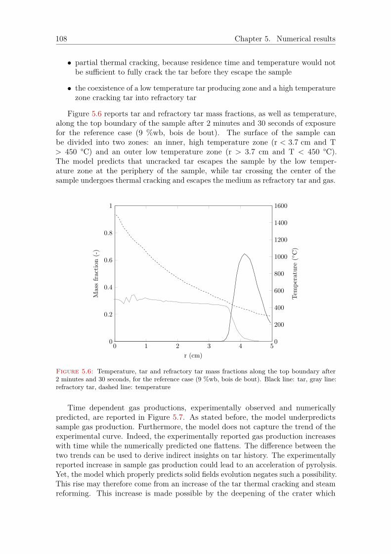
108 Chapter 5. Numerical results
• partial thermal cracking, because residence time and temperature would notbe sufficient to fully crack the tar before they escape the sample
• the coexistence of a low temperature tar producing zone and a high temperaturezone cracking tar into refractory tar
Figure 5.6 reports tar and refractory tar mass fractions, as well as temperature,along the top boundary of the sample after 2 minutes and 30 seconds of exposurefor the reference case (9 %wb, bois de bout). The surface of the sample canbe divided into two zones: an inner, high temperature zone (r < 3.7 cm and T> 450 °C) and an outer low temperature zone (r > 3.7 cm and T < 450 °C).The model predicts that uncracked tar escapes the sample by the low temper-ature zone at the periphery of the sample, while tar crossing the center of thesample undergoes thermal cracking and escapes the medium as refractory tar and gas.
0 1 2 3 4 50
0.2
0.4
0.6
0.8
1
r (cm)
Massfraction
(-)
0
200
400
600
800
1000
1200
1400
1600
Tem
perature
(◦C)
Figure 5.6: Temperature, tar and refractory tar mass fractions along the top boundary after2 minutes and 30 seconds, for the reference case (9 %wb, bois de bout). Black line: tar, gray line:refractory tar, dashed line: temperature
Time dependent gas productions, experimentally observed and numericallypredicted, are reported in Figure 5.7. As stated before, the model underpredictssample gas production. Furthermore, the model does not capture the trend of theexperimental curve. Indeed, the experimentally reported gas production increaseswith time while the numerically predicted one flattens. The difference between thetwo trends can be used to derive indirect insights on tar history. The experimentallyreported increase in sample gas production could lead to an acceleration of pyrolysis.Yet, the model which properly predicts solid fields evolution negates such a possibility.This rise may therefore come from an increase of the tar thermal cracking and steamreforming. This increase is made possible by the deepening of the crater which

5.3. General behaviour 109
induces a higher tar residence time in a high temperature medium. Yet, the model,which only accounts for intra-particular tar thermal cracking, does not predict thisincrease. Altogether, this leads to think that extra particular tar cracking andtar steam reforming play a major role in the evolution of the gaseous productsdistribution. External CFD study would thus be required in order to improvegaseous products distribution prediction.
0 1 2 3 4 50
1
2
3
4
5
Time (min)
Productionrate
(g/min)
Figure 5.7: Experimental and numerical time dependent gas productions, for the reference case(9 %wb, bois de bout). Black line: experimental result, gray line: numerical prediction
Figures 5.6 and 5.7 exhibit oscillations on the numerically predicted tar curves.They are thought to come from pressure solving artefacts presented in Section 4.8.It is especially true for Figure 5.6, where oscillations are limited to the left part ofthe curve. Indeed, this part corresponds to a zone where biomass has undergonepyrolysis and therefore a strong porosity gradient exists.
5.3.3 Char steam gasification
The numerical model confirms that water is forced out of the sample through thehigh temperature char layer. This configuration could allow char steam gasificationto take place inside of the char crater.
Two different mechanisms could explain the computational domain deformation:very low char production, i.e. the produced amount of char would not be sufficientto overpass the deformation criterion (ζ > 0.975) or steam gasification of the charproduced by pyrolysis.
In order to differentiate the importance of the two phenomena, gasificationwas deactivated for a set of simulations. In this condition, no deformation of thecomputational domain could be observed. It can therefore be concluded that theamount of char produced by pyrolysis is sufficient to prevent the porosity to exceed

110 Chapter 5. Numerical results
ωgasi (kg/m3/s)
(a) 9 %wb initial moisture content (b) 55 %wb initial moisture content
Figure 5.8: Gasification reaction rate fields for 9 and 55 %wb initial moisture content cases, after2 minutes and 30 seconds. Colormap: gasification reaction rate
0.975.
Figure 5.8 reports the char steam gasification reaction rate for both 9 and55 %wb initial moisture content cases after 2 minutes and 30 seconds of exposure.Char steam gasification exclusively consumes char very close to the upper boundary,where temperature is high enough. Gasification is therefore the main phenomenonbehind medium ablation.
Char steam gasification is much more intense for high initial moisture contentsamples, with a maximum rate of 8.5 kg/m3/s, while it peaks at 2.5 kg/m3/s for9 %wb initial moisture content samples. Given char steam gasification endother-micity, this difference of intensity explains the lower top surface temperature bothexperimentally observed and numerically predicted for high initial moisture contentsamples (Table 5.2).
5.4 Sensitivity analyses
Three key choices were made during the building steps of the model: the choice ofthe drying model, the choice of the pyrolysis model and the correction to the chosenpyrolysis model. The impact of these choices is here investigated through sensitivityanalyses. For the model choices, it was done by implementing other models andcomparing their predictions. For the correction factor, it was done, classically, bymodifying its value.
5.4.1 Sensitivity to the drying model
The chosen drying model is based on a liquid-vapour equilibrium approach. It isknown to produce high quality results at the price of an heavy implementation anda considerable CPU time load during the simulation. It was chosen to compare

5.4. Sensitivity analyses 111
its predictions to an Arrhenius type drying model featuring vaporisation andcondensation [94]. This model uses a temperature threshold of 95 °C above whichwater evaporates and below which it can condense (Eq. 5.1 and 5.2). Yet, this modeldoes not make the distinction between bound and free waters and does not considertheir motions. Finally, in this model, mass transport physical properties are notaffected by pore water content, i.e. qg = I.
ωlw 7→steam = 5.13 106 exp(87900
ℜT)ρlw if T > 95 ◦C (5.1)
ωsteam 7→lw = 21500 ‖ug‖ρgYsteam if T < 95 ◦C (5.2)
Table 5.3 reports the results of the benchmark between the two drying models(variations being calculated according to Eq. 5.3). For 0 %wb initial moisture contentcase, only minor differences (under 4 %) appear on a global level between the two pre-dictions. Figure 5.9 shows the repartition of the water inside of the sample predictedby the two models. The Arrhenius type model overpredicts the thickness of the areawhere water condenses inside of the sample, while the total amount of water re-tained in the sample is in agreement with liquid-vapour equilibrium model prediction.
Variation =Altertative value - Reference value
Reference value(5.3)
Initial moisture content0 %wb 9 %wb 55 %wb
Surface temperature -0.4 -0.9 3.5Crater depth -2.6 0.0 5Pyrolysis front thickness 0.0 0.0 0.0Time averaged rates:Wood -1.9 -0.5 4.1Water 3.8 -22.4 -38.4Char -1.8 0.0 3.8Gas -1.4 -2.5 5.8Tar -2.5 -1.0 45.2
Table 5.3: Variations (in %) between liquid-vapour equilibrium model and Arrhenius type model
For 9 and 55 %wb initial moisture content cases, Arrhenius type model substan-tially underpredicts the amount of water leaving the sample (-22.4 and -38.4 %,respectively). These underpredictions are explained by the fact that for these casesArrhenius type model overpredicts the amount of water that condenses inside of thesample (Fig. 5.10). Indeed, the Arrhenius type model is not capable of limiting theamount that condenses at a given point because it does not take into account thelimit imposed by the liquid-vapour equilibrium. Therefore, even if the same amountof water is initially vaporised, a higher amount of water is retained by the sample
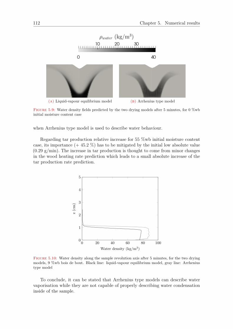
112 Chapter 5. Numerical results
ρwater (kg/m3)
(a) Liquid-vapour equilibrium model (b) Arrhenius type model
Figure 5.9: Water density fields predicted by the two drying models after 5 minutes, for 0 %wbinitial moisture content case
when Arrhenius type model is used to describe water behaviour.
Regarding tar production relative increase for 55 %wb initial moisture contentcase, its importance (+ 45.2 %) has to be mitigated by the initial low absolute value(0.29 g/min). The increase in tar production is thought to come from minor changesin the wood heating rate prediction which leads to a small absolute increase of thetar production rate prediction.
0 20 40 60 80 1000
1
2
3
4
5
Water density (kg/m3)
z(cm)
Figure 5.10: Water density along the sample revolution axis after 5 minutes, for the two dryingmodels, 9 %wb bois de bout. Black line: liquid-vapour equilibrium model, gray line: Arrheniustype model
To conclude, it can be stated that Arrhenius type models can describe watervaporisation while they are not capable of properly describing water condensationinside of the sample.

5.4. Sensitivity analyses 113
5.4.2 Sensitivity to b fitting parameter
During the building of the model a fitting parameter b was added to correct the charyield predicted by the pyrolysis scheme (Fig. 4.3 and Table 4.3). In order to assessfor the impact of this choice, a sensitivity analysis to this parameter was led. The bparameter was varied between -50 to +50 %, with a reference value of 2. One shouldnote that the -50 % case corresponds to b = 1, which is the actual pyrolysis schemewithout modification.
b factor variation-50 % -20 % -10 % +10 % +20 % +50 %
Surface temperature -5.0 -1.0 0.0 0.0 0.0 -1.0Crater depth 5.0 3.0 0.0 0.0 -3.0 -3.0Pyrolysis front thickness -25 0 0 25 25 50Time averaged rates:Wood -6.0 -2.0 -1.0 1.0 2.0 5.0Water -5.0 -1.0 -1.0 1.0 1.0 3.0Char -49.0 -19.0 -9.0 10.0 19.0 46.0Gas 5.0 2.0 1.0 -1.0 -2.0 -5.0Tar 8.0 2.0 1.0 -1.0 -2.0 -6.0
Table 5.4: Variations (in %) for different b parameter values with respect to the reference valueb = 2
Table 5.4 reports variations for different b parameter values in the reference caseconditions, i.e. 9 %wb, bois de bout. The observed outputs can be divided into twobroad categories: the ones strongly varying with b and the ones robust with respectof b.
b factor has a strong impact on char production rate and pyrolysis front thickness.An increase of b implies, as expected, an increase in char production rate. Thedependency between b and the char production is linear. The pyrolysis front alsothickens with an increase of the b factor. These two results are explained by the factthat the b factor directly increase the intermediate solid production and therefore thechar production. Pyrolysis front thickness exhibits strong variations. Even thoughthe trend is reasonable, absolute variation values have to be mitigated consideringtheir front thickness calculation method. Indeed front thickness is evaluated withonly one significant digit, therefore rounding error can yield important variation. e.g.+25 % for an increase from 4 to 5 mm.
b factor has a minor, yet existing, impact on crater depth, wood consumption rateand water, gas and tar production rates. An increase of b induces a reduction in thecrater depth, which is thought to be a consequence of the thickening of the pyrolysisfront. It also modifies the product distribution: with an increase of b, more wood inconsumed, more water is released while less gas and tar are produced. The increasein wood consumption and water release can be explained by the exothermicity

114 Chapter 5. Numerical results
of the intermediate solid to char conversion reaction. Therefore, producing moreintermediate solid leads to an increase of the heat released inside of the sample. Thisheat, in turn, is used to power drying and pyrolysis.
b factor impact on gas and tar production rate is surprisingly low. Even if bmodifies the distribution of wood pyrolysis primary products, gas and tar productionrates are very robust, with variations below 8 % for ±50 % variations of b value.This result shows that the addition of b did not drastically modify the model results.Therefore, it can be stated that the b factor modifies the char production with noside effects on the simulation results.
The next step would be to determine a best fitting value for the correction factorb. Yet, given the fact that b lacks experimental validation, it was chosen not todetermine it with more than one significant digit. It was therefore chosen to keep itsvalue to 2.
5.4.3 Sensitivity to the pyrolysis model
Similarly to the impact of the choice of the drying model, the importance of thechoice of the pyrolysis model has been assessed by using an alternative pyrolysismodel (Fig. 5.11 and Table 5.5). The alternative model was derived for beech woodand was validated against experimental results for lower pyrolysis temperatures andheating rates than the one chosen to build the model [20]. The production of waterby wood pyrolysis was taken into account using the same method as for the referencemodel [63]. Except for the frequency factors and activation energy values, severaldifferences exists between the two models, the second model:
• does not feature an intermediate solid pseudo-specie that mediates char pro-duction
• describes pyrolysis as an entirely endothermic process with no exothermic lignindegradation
• does not take tar repolymerisation reactions into account
Number Reaction A (1/s) Ea (kJ/mol) ∆h (kJ/kg) Reference
1’ Wood 7→ steam 2.0 108 × a 133 -418 [20, 63]2’ Wood 7→ gas 1.3 108 140 -418 [20]3’ Wood 7→ tar 2.0 108 × (1-a) 133 -418 [20, 63]4’ Wood 7→ char 1.08 107 121 -418 [20]5’ Tar 7→ gas 9.6 105 144 42 [20, 55]6’ Tar 7→ refractory tar 5.2 105 144 42 [20, 55]
Table 5.5: Alternative kinetic parameters for beech wood pyrolysis. a = 0.219 [63]
Table 5.6 reports the results of the benchmark between the two pyrolysismodels. Significant discrepancies arise from this comparison. The alternative model

5.4. Sensitivity analyses 115
Water Steam
Gas
Wood Tar
Refractory tar
Char
k′
2
k′
3
k′
4
k′
5
k′
7
k9
k′
1
Figure 5.11: Alternative biomass pyrolysis scheme
substantially underpredicts wood consumption, water, char and gas production rates,as well as crater depth, while it overpredicts tar production rate.
The poor quality of the predictions is attributed to the endothermic latent heatsassociated with biomass degradation in the alternative model. Indeed, the alternativemodel does not take into account lignin exothermic degradation. Hence, the pyrolysisis endothermic, while it should be athermic. Pyrolysis acting as an heat sink, itreduces the amount of power available to dry the medium and degrade wood. Hence,wood consumption, water, char and gas production rates and crater depth are lowered.
Tar production rate overprediction is thought to be linked to a skewed repartitionof the pyrolysis gaseous products highly favouring tar over gas.
Initial moisture content0 %wb 9 %wb 55 %wb
Surface temperature 0.0 -0.1 3.7Crater depth -17.9 -18.9 -20.0Pyrolysis front thickness 0.0 0.0 100Time averaged rates:Wood -26.7 -23.7 -15.8Water -26.9 -10.3 -3.4Char -18.2 -14.2 -3.8Gas -67.0 -66.4 -61.3Tar 13.5 22.2 66.6
Table 5.6: Variations (in %) between the two pyrolysis models
Conclusion
This chapter presented the numerical model predictions. First, the model con-struction assumptions were validated. Key dimensionless numbers were shown

116 Chapter 5. Numerical results
not to exceed critical values. Then, numerical predictions were confronted to theexperimental observations. The agreement between the numerical and experimentalresults is good. Based on the model predicted behaviour of biomass, furtherunderstanding of biomass degradation under high solar heat flux was derived.
Drying, pyrolysis and gasification fronts are present at the same time inside ofthe sample. The coexistence of these three thermochemical fronts leads to physicalcouplings. The major coupling being char gasification by the steam produced fromdrying of the sample. The model confirms that char-steam gasification is the mainphenomenon behind medium ablation. The model also allows to envision the factthat tar thermal history is not limited to the residence time inside of the sample. Itis very likely that they undergo thermal cracking and steam reforming after leavingthe sample.
From a modelling perspective, it can be concluded from sensitivity analysesresults that Arrhenius type models are not fitted for precise intra-particular waterbehaviour description. Indeed, they tend to mispredict the amount of water thatcondenses in the cold zones of the sample. These models may still be useful todescribe high temperature drying whenever steam condensation is not possible.
Furthermore, the influence of the char yield correction factor was assessed. Thisadjustment has only a minor impact on the model behaviour, i.e. it modifies theamount of char that is produced by the sample with no side-effects on the otheroutputs predicted by the model. Sensitivity analyses have also shown that the choiceof the biomass degradation scheme is key to properly model biomass behaviour underhigh solar heat flux. The use of a model validated for experimental conditions whichare far from the simulated conditions leads to erroneous predictions.

Conclusion
Conclusion
Over the last three years, this PhD work tried to offer a better understanding of theinteraction between biomass and concentrated solar energy. It started with an idea:combining these two energy sources so that they could compensate one another’sweaknesses, i.e. biomass endothermic gasification and solar energy intermittence.In addition to the general behaviour of biomass in itself, the potentiality of thiscombination raised several questions. Biomass high heating rates could indeed leadto:
• fast sample drying, inducing to high internal pressure and potential mechanicalfailure
• very little char production and therefore rapid ablation of the medium
High achieved temperatures could enable:
• tar thermal cracking and steam reforming, while produced char could undergosteam gasification
• char thermal annealing
• carbon sublimation
It was chosen to resort on a classical approach to tackle these questions. First,literature on biomass and concentrated solar energy was reviewed. As a first step, anexperimental device allowing to expose the biomass to concentrated radiative powerwas built. Then, this device was calibrated and operated and experimental resultswere analysed. As a second step, a numerical model describing biomass degradationunder high solar heat flux was developed. This model was validated against theexperimental results before being used to derive a better understanding of biomassbehaviour under high solar heat flux.
The review of existing literature showed a lack of previous work on the specificsubject of biomass degradation under high solar heat flux at the sample scale. Itnevertheless emphasizes the three steps of biomass degradation: drying, pyrolysis
117

118 Conclusion
and gasification. These three main steps are complex in essence and influencingone another. Each of them has been widely studied. Yet, few studies focuses ontwo at the same time, while none encompassed the three of them in their scopes.This review of literature has allowed for a better understanding of these individualsteps and the potential couplings between them. It has also been the opportunity tohighlight the different modelling strategies developed to describe these phenomena.Finally, on a very practical level, this review of literature has oriented toward to usebeech wood (Fagus sylvatica) as model biomass, because it is commonly used, whichhas two considerable advantages: allowing for comparison with other studies andincreasing the availability of thermo-physical properties mandatory for numericalmodelling.
A new experimental device allowing to expose thermally thick beech wood samplesto radiative heat flux higher than 1000 kW/m2 was built from scratch. Sampleswere designed in such a way that they would allow to explore the impact of fiberorientation and initial moisture content on beech wood behaviour under high solarheat flux. Samples representing two extreme wood fiber orientations were designed:bois de bout and bois de fil configurations. Samples with three different initialmoisture contents were produced: 0 %wb corresponding to oven dried samples, 9 %wbaccounting for samples stabilized under ambient conditions and 55 %wb emulatingwood after cutting. Finally, special care was taken in calibrating this device, lead-ing to the development of a new method of calibration for solar concentrating systems.
Using this experimental device, an original behaviour has been highlighted.Under high radiative heat flux, sample geometry evolves dramatically over a run. Acrater which mirrors incident heat flux distribution is formed. Two mechanisms ofcrater formation have been proposed: one involving sample shrinkage and mechanicalfailure for low initial moisture content sample, the other relying on char steamgasification for high initial moisture content samples. Furthermore, produced charsdo not undergo thermal annealing and exhibit high oxygen and hydrogen contents.Finally, achieved temperatures were high enough to promote tar thermal cracking,but not sufficient to achieve carbon sublimation.
Regarding the effect of wood fiber orientation relative to the incident heat flux, theproduced results show that varying the sample orientation between the two extremahas only a minor effect on the sample behaviour. On the contrary, sample initialmoisture content was shown to be of considerable importance. It was highlightedthat samples containing high initial moisture content undergo char gasification.They produce 2.6 times more gas - per unit of converted dry wood - than low initialmoisture content samples. Furthermore, this gas is richer in H2. Nevertheless, theinput power retained in the products of high initial moisture content samples isquite low, around 59 %. The tar yield is close to zero. It has also been shown thatsamples containing no water produce much more tar than moist samples. For thesesamples solar pyro-gasification exhibits a very good energy conversion efficiency: therecoverable products contain 90 % of the inputs (solar + wood) power. Furthermore,the power recovered in the outputs exceeds the wood input power alone, in every
119
configuration. It means that some of the incident radiative power has been convertedinto chemical form. The fraction of the incident radiative power captured can be ashigh as 72 % for 0 %wb, bois de bout samples.
In order to derive further insights on biomass behaviour under high solar heat flux,a numerical model describing samples under high heat flux exposure was developed.This model is based on three main conservation equations: mass, momentum andheat balances. These equations are coupled with liquid-vapour equilibrium dryingmodel and pseudo-species biomass degradation model. Assumptions made to writethese equations are defended using dimensionless numbers. Because of biomass solargasification specific nature, i.e. medium gasification and radiation penetration, itwas mandatory to develop and implement special strategies to describe mediumshape evolution and incident heat flux penetration into the crater geometry.
As a validation step, the model construction assumptions were validated andthe numerical predictions were confronted to the experimental observations. Theagreement between the numerical and experimental results is good. Based on themodel predicted behaviour, further understanding of biomass behaviour under highsolar heat flux was derived. The model confirms that the gasification of char bythe steam produced during drying of the sample is the main phenomenon behindmedium ablation. It also allows to envision the fact that tar thermal history isnot limited to the residence time inside of the sample. It is very likely that theyundergo thermal cracking and steam reforming after leaving the sample. In addition,sensitivity analyses revealed that Arrhenius type models are not fitted for preciseintra-particular water behaviour description and that the choice of the pyrolysisscheme is key to properly model biomass behaviour under high solar heat flux.
In this attempt to better understand beech wood behaviour under high solar heatflux, it was shown that:
• even for high initial moisture content samples, water vaporisation did not sufficeto lead to sample mechanical failure
• the achieved heating rates were not high enough for the pyrolysis to yieldalmost no char
• tar thermal cracking and steam reforming, as well as char gasification play amajor role during biomass exposition to high solar heat flux
• an exposure time of several minutes is too short for char to undergo thermalannealing even under high radiative heat flux
• reached temperatures were not high enough to enable carbon sublimation
As a general conclusion, based on the results of this work, it can be stated thatthe solar pyro-gasification of moist biomass is interesting for enhanced direct H2
production with reduced tar yield, while solar pyro-gasification of dry biomass isadvantageous in the perspective of solar to fuel energy conversion. In any of these

120 Conclusion
configurations, solar pyro-gasification process allows to capture solar energy inchemical form.

121
Appendices

APPENDIX ATar analysis
Tar collected in the cotton trap were analysed at CIRAD laboratory. They werefirst desorbed in acetone then analysed using gas chromatography coupled with massspectrometry. Cotton was analysed to provide blank test results (Fig. A.1). 0 and9 %wb initial moisture content samples tar were analysed twice in order to asses forrun to tun repeatability (Fig. A.2 to A.5).
123

124 Appendix A. Tar analysis
RAPPORT D'ANALYSE GC-MS
Nom de l'échantillon : Blanc
Date de l'expérience : 24 février 2015
Date de l'analyse : 24 février 2015
Date de traitement : 15 juillet 2015
Colonne : DB1701 - Cpsil19CB 14% cyanopropylphényl et 86% dimethylpolysiloxanne
Chromatographe : GC Agilent 6890
Détecteur : Spectromètre de Masse Agilent 5975
CAS Alcools [] mg/L CAS Phenols [] mg/L
67-56-1 Methanol <LQ (200) 108-95-2 Phenol <LQ (1)
95-48-7 Phenol-2-methyl <LQ (1)
Total Alcools 0.00 106-44-5 et 108-39-4 Phenol-3-methyl+Phenol-4-methyl <LQ (2)
95-65-8 3,4-dimethylphenol <LQ (1)
CAS Aldehydes et cétones [] mg/L 105-67-9 2,4-dimethylphenol <LQ (1)
50-00-0 Formaldehyde 68.71 90-15-3 1-naphthalenol <LQ (1)
75-07-0 Acetaldehyde 40.67 135-19-3 2-naphthalenol <LQ (1)
23147-58-2 Glycolaldehyde <LQ (50) 123-31-9 Hydroquinone <LQ (1)
116-09-6 2-Propanone,1-hydroxy- <LQ (50)
930-30-3 2-cyclopenten-1-one <LQ (1) Total phénols 0.00
2758-18-1 2-cyclopenten-1-one-3-methyl <LQ (1)
5077-67-8 2-Butanone,1-hydroxy- <LQ (50) CAS Guaiacols [] mg/L
765-70-8 3-methyl-1,2-cyclopentanedione <LQ (1) 90-05-1 Phenol-2-methoxy <LQ (1)
10493-98-8 2-hydroxy-2-cyclopenten-1-one <LQ (1) 93-51-6 Phenol-2-methoxy-4-methyl <LQ (1)
592-20-1 1-acetyloxy-2-propanone <LQ (1) 91-10-1 2,6-dimethoxyphenol <LQ (1)
2785-89-9 Phenol-4-ethyl-2-methoxy <LQ (1)
Total Aldehydes et cétones 109.38 97-53-0 Eugenol <LQ (1)
97-54-1 Isoeugenol <LQ (1)
CAS Acides [] mg/L 7786-61-0 2-methoxy-4-vinylphenol <LQ (1)
64-18-6 Formic_acid <LQ (100) 4812-20-8 2-isopropoxyphenol <LQ (1)
64-19-7 Acetic_acid <LQ (50)
79-09-4 Propionic_acid <LQ (50) Total Guaiacols 0.00
Total acides 0.00 CAS HAPs [] mg/L
91-20-3 Naphthalene <LQ (1)
CAS Furanes [] mg/L 90-12-0 Naphthalene-1-methyl <LQ (1)
98-01-1 Furfural <LQ (1) 91-57-6 Naphthalene-2-methyl <LQ (1)
98-00-0 2-furanmethanol <LQ (1) 208-96-8 Acenaphthylene <LQ (1)
271-89-6 Benzofuran <LQ (1) 83-32-9 Acenaphthene <LQ (1)
620-02-0 2-furancarboxaldehyde,5-methyl <LQ (1) 86-73-7 Fluorene <LQ (1)
625-86-5 2,5-dimethylfuran <LQ (1) 85-01-8 Phenanthrene <LQ (1)
67-47-0 5-hydroxymethylfurfural <LQ (10) 120-12-7 Anthracene <LQ (1)
206-44-0 Fluoranthene <LQ (1)
Total furanes 0.00 129-00-0 Pyrene <LQ (1)
56-55-3 Benzo(a)anthracene <LQ (1)
CAS Aromatiques azotés [] mg/L 218-01-9 Chrysene <LQ (1)
110-86-1 Pyridine <LQ (4) 205-99-2 Benzo(b)luoranthene <LQ (1)
109-06-8 Pyridine-2-methyl <LQ (1) 207-08-9 Benzo(k)luoranthene <LQ (1)
91-22-5 Quinoline <LQ (1) 50-32-8 Benzo(a)pyrene <LQ (1)
119-65-3 Isoquinoline <LQ (1) 191-24-2 Benzo(ghi)perylene <LQ (1)
53-70-3 Dibenzo(ah)anthracene <LQ (1)
Total aromatiques azotés 0.00 193-39-5 Indeno(123cd)pyrene <LQ (1)
CAS Aromatiques [] mg/L Total HAPs 0.00
71-43-2 Benzene <LQ (2)
108-88-3 Toluene <LQ (1) CAS Terpenes [] mg/L
100-41-4 Ethylbenzene <LQ (2) 7785-70-8 1-R-a-pinene <LQ (1)
108-38-3 et 106-42-3 (m+p)-xylene <LQ (1)
95-47-6 O-xylene <LQ (1) Total Sucres 0.00
100-42-5 Styrene <LQ (1)
95-13-6 Indene <LQ (1) [] mg/L
2177-47-1 2-methylindene <LQ (1)
536-74-3 Phenylethyne <LQ (1)
Total général 109.38Total aromatiques 0.00
CAS Sucres [] mg/L
Figure A.1: Virgin cotton analysis

125
RAPPORT D'ANALYSE GC-MS
Nom de l'échantillon : Run 68
Date de l'expérience : 29/06/2015
Date de l'analyse : 29 juin 2015
Date de traitement : 15 juillet 2015
Colonne : DB1701 - Cpsil19CB 14% cyanopropylphényl et 86% dimethylpolysiloxanne
Chromatographe : GC Agilent 6890
Détecteur : Spectromètre de Masse Agilent 5975
CAS Alcools [] mg/L CAS Phenols [] mg/L
67-56-1 Methanol <LQ (200) 108-95-2 Phenol 31.39
95-48-7 Phenol-2-methyl 6.05
Total Alcools 0.00 106-44-5 et 108-39-4 Phenol-3-methyl+Phenol-4-methyl 10.98
95-65-8 3,4-dimethylphenol <LQ (1)
CAS Aldehydes et cétones [] mg/L 105-67-9 2,4-dimethylphenol 2.42
50-00-0 Formaldehyde <LQ (50) 90-15-3 1-naphthalenol <LQ (1)
75-07-0 Acetaldehyde 30.34 135-19-3 2-naphthalenol <LQ (1)
23147-58-2 Glycolaldehyde <LQ (200) 123-31-9 Hydroquinone 2.80
116-09-6 2-Propanone,1-hydroxy- <LQ (50)
930-30-3 2-cyclopenten-1-one 6.47 Total phénols 53.64
2758-18-1 2-cyclopenten-1-one-3-methyl 3.44
5077-67-8 2-Butanone,1-hydroxy- <LQ (50) CAS Guaiacols [] mg/L
765-70-8 3-methyl-1,2-cyclopentanedione 9.14 90-05-1 Phenol-2-methoxy 1.83
10493-98-8 2-hydroxy-2-cyclopenten-1-one <LQ (4) 93-51-6 Phenol-2-methoxy-4-methyl 1.44
592-20-1 1-acetyloxy-2-propanone <LQ (1) 91-10-1 2,6-dimethoxyphenol 3.97
2785-89-9 Phenol-4-ethyl-2-methoxy 0.74
Total Aldehydes et cétones 49.39 97-53-0 Eugenol <LQ (1)
97-54-1 Isoeugenol 0.62
CAS Acides [] mg/L 7786-61-0 2-methoxy-4-vinylphenol 2.29
64-18-6 Formic_acid <LQ (100) 4812-20-8 2-isopropoxyphenol <LQ (1)
64-19-7 Acetic_acid 198.54
79-09-4 Propionic_acid <LQ (50) Total Guaiacols 10.89
Total acides 198.54 CAS HAPs [] mg/L
91-20-3 Naphthalene 1.27
CAS Furanes [] mg/L 90-12-0 Naphthalene-1-methyl <LQ (1)
98-01-1 Furfural 5.76 91-57-6 Naphthalene-2-methyl <LQ (1)
98-00-0 2-furanmethanol <LQ (1) 208-96-8 Acenaphthylene 2.02
271-89-6 Benzofuran <LQ (1) 83-32-9 Acenaphthene 0.84
620-02-0 2-furancarboxaldehyde,5-methyl 1.38 86-73-7 Fluorene <LQ (1)
625-86-5 2,5-dimethylfuran <LQ (1) 85-01-8 Phenanthrene 4.05
67-47-0 5-hydroxymethylfurfural <LQ (10) 120-12-7 Anthracene 1.04
206-44-0 Fluoranthene 3.11
Total furanes 7.14 129-00-0 Pyrene 3.56
56-55-3 Benzo(a)anthracene <LQ (1)
CAS Aromatiques azotés [] mg/L 218-01-9 Chrysene <LQ (1)
110-86-1 Pyridine <LQ (4) 205-99-2 Benzo(b)luoranthene <LQ (1)
109-06-8 Pyridine-2-methyl <LQ (1) 207-08-9 Benzo(k)luoranthene <LQ (1)
91-22-5 Quinoline <LQ (1) 50-32-8 Benzo(a)pyrene <LQ (1)
119-65-3 Isoquinoline <LQ (1) 191-24-2 Benzo(ghi)perylene <LQ (1)
53-70-3 Dibenzo(ah)anthracene <LQ (1)
Total aromatiques azotés 0.00 193-39-5 Indeno(123cd)pyrene <LQ (1)
CAS Aromatiques [] mg/L Total HAPs 15.89
71-43-2 Benzene <LQ (2)
108-88-3 Toluene <LQ (1) CAS Terpenes [] mg/L
100-41-4 Ethylbenzene <LQ (2) 7785-70-8 1-R-a-pinene <LQ (1)
108-38-3 et 106-42-3 (m+p)-xylene <LQ (1)
95-47-6 O-xylene <LQ (1) Total Sucres 0.00
100-42-5 Styrene <LQ (1)
95-13-6 Indene <LQ (1) [] mg/L
2177-47-1 2-methylindene <LQ (1)
536-74-3 Phenylethyne <LQ (1)
Total général 352.81Total aromatiques 0.00
CAS Sucres [] mg/L
Figure A.2: 0 %wb initial moisture content sample tar analysis, run 1

126 Appendix A. Tar analysis
RAPPORT D'ANALYSE GC-MS
Nom de l'échantillon : Run 69
Date de l'expérience : 29/06/2015
Date de l'analyse : 29 juin 2015
Date de traitement : 15 juillet 2015
Colonne : DB1701 - Cpsil19CB 14% cyanopropylphényl et 86% dimethylpolysiloxanne
Chromatographe : GC Agilent 6890
Détecteur : Spectromètre de Masse Agilent 5975
CAS Alcools [] mg/L CAS Phenols [] mg/L
67-56-1 Methanol <LQ (200) 108-95-2 Phenol 27.51
95-48-7 Phenol-2-methyl 5.12
Total Alcools 0.00 106-44-5 et 108-39-4 Phenol-3-methyl+Phenol-4-methyl 8.71
95-65-8 3,4-dimethylphenol <LQ (1)
CAS Aldehydes et cétones [] mg/L 105-67-9 2,4-dimethylphenol 1.78
50-00-0 Formaldehyde <LQ (50) 90-15-3 1-naphthalenol <LQ (1)
75-07-0 Acetaldehyde <LQ (50) 135-19-3 2-naphthalenol <LQ (1)
23147-58-2 Glycolaldehyde <LQ (200) 123-31-9 Hydroquinone 3.27
116-09-6 2-Propanone,1-hydroxy- <LQ (50)
930-30-3 2-cyclopenten-1-one 6.46 Total phénols 46.40
2758-18-1 2-cyclopenten-1-one-3-methyl 2.22
5077-67-8 2-Butanone,1-hydroxy- <LQ (50) CAS Guaiacols [] mg/L
765-70-8 3-methyl-1,2-cyclopentanedione <LQ (1) 90-05-1 Phenol-2-methoxy <LQ (1)
10493-98-8 2-hydroxy-2-cyclopenten-1-one <LQ (4) 93-51-6 Phenol-2-methoxy-4-methyl 0.88
592-20-1 1-acetyloxy-2-propanone <LQ (1) 91-10-1 2,6-dimethoxyphenol 4.16
2785-89-9 Phenol-4-ethyl-2-methoxy <LQ (1)
Total Aldehydes et cétones 8.68 97-53-0 Eugenol <LQ (1)
97-54-1 Isoeugenol 0.37
CAS Acides [] mg/L 7786-61-0 2-methoxy-4-vinylphenol <LQ (1)
64-18-6 Formic_acid <LQ (100) 4812-20-8 2-isopropoxyphenol <LQ (1)
64-19-7 Acetic_acid 195.87
79-09-4 Propionic_acid <LQ (50) Total Guaiacols 5.41
Total acides 195.87 CAS HAPs [] mg/L
91-20-3 Naphthalene 1.21
CAS Furanes [] mg/L 90-12-0 Naphthalene-1-methyl <LQ (1)
98-01-1 Furfural 5.74 91-57-6 Naphthalene-2-methyl <LQ (1)
98-00-0 2-furanmethanol <LQ (1) 208-96-8 Acenaphthylene 1.10
271-89-6 Benzofuran <LQ (1) 83-32-9 Acenaphthene <LQ (1)
620-02-0 2-furancarboxaldehyde,5-methyl 1.12 86-73-7 Fluorene <LQ (1)
625-86-5 2,5-dimethylfuran <LQ (1) 85-01-8 Phenanthrene 4.65
67-47-0 5-hydroxymethylfurfural <LQ (10) 120-12-7 Anthracene 1.09
206-44-0 Fluoranthene 3.92
Total furanes 6.87 129-00-0 Pyrene 4.55
56-55-3 Benzo(a)anthracene <LQ (1)
CAS Aromatiques azotés [] mg/L 218-01-9 Chrysene <LQ (1)
110-86-1 Pyridine <LQ (4) 205-99-2 Benzo(b)luoranthene <LQ (1)
109-06-8 Pyridine-2-methyl <LQ (1) 207-08-9 Benzo(k)luoranthene <LQ (1)
91-22-5 Quinoline <LQ (1) 50-32-8 Benzo(a)pyrene <LQ (1)
119-65-3 Isoquinoline <LQ (1) 191-24-2 Benzo(ghi)perylene <LQ (1)
53-70-3 Dibenzo(ah)anthracene <LQ (1)
Total aromatiques azotés 0.00 193-39-5 Indeno(123cd)pyrene <LQ (1)
CAS Aromatiques [] mg/L Total HAPs 16.51
71-43-2 Benzene <LQ (2)
108-88-3 Toluene <LQ (1) CAS Terpenes [] mg/L
100-41-4 Ethylbenzene <LQ (2) 7785-70-8 1-R-a-pinene <LQ (1)
108-38-3 et 106-42-3 (m+p)-xylene <LQ (1)
95-47-6 O-xylene <LQ (1) Total Sucres 0.00
100-42-5 Styrene <LQ (1)
95-13-6 Indene <LQ (1) [] mg/L
2177-47-1 2-methylindene <LQ (1)
536-74-3 Phenylethyne <LQ (1)
Total général 295.93Total aromatiques 0.00
CAS Sucres [] mg/L
Figure A.3: 0 %wb initial moisture content sample tar analysis, run 2

127
RAPPORT D'ANALYSE GC-MS
Nom de l'échantillon : Run 42
Date de l'expérience : 25 février 2015
Date de l'analyse : 25 février 2015
Date de traitement : 15 juillet 2015
Colonne : DB1701 - Cpsil19CB 14% cyanopropylphényl et 86% dimethylpolysiloxanne
Chromatographe : GC Agilent 6890
Détecteur : Spectromètre de Masse Agilent 5975
CAS Alcools [] mg/L CAS Phenols [] mg/L
67-56-1 Methanol <LQ (200) 108-95-2 Phenol 9.40
95-48-7 Phenol-2-methyl <LQ (1)
Total Alcools 0.00 106-44-5 et 108-39-4 Phenol-3-methyl+Phenol-4-methyl 4.52
95-65-8 3,4-dimethylphenol <LQ (1)
CAS Aldehydes et cétones [] mg/L 105-67-9 2,4-dimethylphenol 0.71
50-00-0 Formaldehyde <LQ (50) 90-15-3 1-naphthalenol 0.86
75-07-0 Acetaldehyde <LQ (50) 135-19-3 2-naphthalenol 0.77
23147-58-2 Glycolaldehyde <LQ (50) 123-31-9 Hydroquinone 2.21
116-09-6 2-Propanone,1-hydroxy- <LQ (50)
930-30-3 2-cyclopenten-1-one <LQ (1) Total phénols 18.48
2758-18-1 2-cyclopenten-1-one-3-methyl 0.96
5077-67-8 2-Butanone,1-hydroxy- <LQ (50) CAS Guaiacols [] mg/L
765-70-8 3-methyl-1,2-cyclopentanedione 5.54 90-05-1 Phenol-2-methoxy <LQ (1)
10493-98-8 2-hydroxy-2-cyclopenten-1-one <LQ (1) 93-51-6 Phenol-2-methoxy-4-methyl <LQ (1)
592-20-1 1-acetyloxy-2-propanone <LQ (1) 91-10-1 2,6-dimethoxyphenol 3.56
2785-89-9 Phenol-4-ethyl-2-methoxy <LQ (1)
Total Aldehydes et cétones 6.50 97-53-0 Eugenol <LQ (1)
97-54-1 Isoeugenol 1.96
CAS Acides [] mg/L 7786-61-0 2-methoxy-4-vinylphenol <LQ (1)
64-18-6 Formic_acid <LQ (100) 4812-20-8 2-isopropoxyphenol <LQ (1)
64-19-7 Acetic_acid 142.37
79-09-4 Propionic_acid <LQ (50) Total Guaiacols 5.52
Total acides 142.37 CAS HAPs [] mg/L
91-20-3 Naphthalene <LQ (1)
CAS Furanes [] mg/L 90-12-0 Naphthalene-1-methyl <LQ (1)
98-01-1 Furfural <LQ (1) 91-57-6 Naphthalene-2-methyl <LQ (1)
98-00-0 2-furanmethanol <LQ (1) 208-96-8 Acenaphthylene 6.08
271-89-6 Benzofuran <LQ (1) 83-32-9 Acenaphthene 1.15
620-02-0 2-furancarboxaldehyde,5-methyl <LQ (1) 86-73-7 Fluorene 3.26
625-86-5 2,5-dimethylfuran <LQ (1) 85-01-8 Phenanthrene 12.83
67-47-0 5-hydroxymethylfurfural <LQ (10) 120-12-7 Anthracene 3.16
206-44-0 Fluoranthene 5.93
Total furanes 0.00 129-00-0 Pyrene 6.24
56-55-3 Benzo(a)anthracene <LQ (1)
CAS Aromatiques azotés [] mg/L 218-01-9 Chrysene <LQ (1)
110-86-1 Pyridine <LQ (4) 205-99-2 Benzo(b)luoranthene <LQ (1)
109-06-8 Pyridine-2-methyl <LQ (1) 207-08-9 Benzo(k)luoranthene <LQ (1)
91-22-5 Quinoline <LQ (1) 50-32-8 Benzo(a)pyrene <LQ (1)
119-65-3 Isoquinoline <LQ (1) 191-24-2 Benzo(ghi)perylene <LQ (1)
53-70-3 Dibenzo(ah)anthracene <LQ (1)
Total aromatiques azotés 0.00 193-39-5 Indeno(123cd)pyrene <LQ (1)
CAS Aromatiques [] mg/L Total HAPs 38.64
71-43-2 Benzene <LQ (2)
108-88-3 Toluene <LQ (1) CAS Terpenes [] mg/L
100-41-4 Ethylbenzene <LQ (2) 7785-70-8 1-R-a-pinene <LQ (1)
108-38-3 et 106-42-3 (m+p)-xylene <LQ (1)
95-47-6 O-xylene <LQ (1) Total Sucres 0.00
100-42-5 Styrene <LQ (1)
95-13-6 Indene <LQ (1) [] mg/L
2177-47-1 2-methylindene <LQ (1)
536-74-3 Phenylethyne <LQ (1)
Total général 211.50Total aromatiques 0.00
CAS Sucres [] mg/L
Figure A.4: 9 %wb initial moisture content sample tar analysis, run 1

128 Appendix A. Tar analysis
RAPPORT D'ANALYSE GC-MS
Nom de l'échantillon : Run 44
Date de l'expérience : 25 février 2015
Date de l'analyse : 25 février 2015
Date de traitement : 15 juillet 2015
Colonne : DB1701 - Cpsil19CB 14% cyanopropylphényl et 86% dimethylpolysiloxanne
Chromatographe : GC Agilent 6890
Détecteur : Spectromètre de Masse Agilent 5975
CAS Alcools [] mg/L CAS Phenols [] mg/L
67-56-1 Methanol <LQ (200) 108-95-2 Phenol 13.05
95-48-7 Phenol-2-methyl 0.77
Total Alcools 0.00 106-44-5 et 108-39-4 Phenol-3-methyl+Phenol-4-methyl 6.25
95-65-8 3,4-dimethylphenol <LQ (1)
CAS Aldehydes et cétones [] mg/L 105-67-9 2,4-dimethylphenol 1.02
50-00-0 Formaldehyde <LQ (50) 90-15-3 1-naphthalenol 1.07
75-07-0 Acetaldehyde <LQ (50) 135-19-3 2-naphthalenol 1.07
23147-58-2 Glycolaldehyde 149.37 123-31-9 Hydroquinone 3.64
116-09-6 2-Propanone,1-hydroxy- 48.01
930-30-3 2-cyclopenten-1-one 1.37 Total phénols 26.87
2758-18-1 2-cyclopenten-1-one-3-methyl 1.78
5077-67-8 2-Butanone,1-hydroxy- <LQ (50) CAS Guaiacols [] mg/L
765-70-8 3-methyl-1,2-cyclopentanedione 9.92 90-05-1 Phenol-2-methoxy <LQ (1)
10493-98-8 2-hydroxy-2-cyclopenten-1-one <LQ (1) 93-51-6 Phenol-2-methoxy-4-methyl <LQ (1)
592-20-1 1-acetyloxy-2-propanone <LQ (1) 91-10-1 2,6-dimethoxyphenol 5.91
2785-89-9 Phenol-4-ethyl-2-methoxy <LQ (1)
Total Aldehydes et cétones 210.45 97-53-0 Eugenol 0.33
97-54-1 Isoeugenol 2.93
CAS Acides [] mg/L 7786-61-0 2-methoxy-4-vinylphenol <LQ (1)
64-18-6 Formic_acid <LQ (100) 4812-20-8 2-isopropoxyphenol <LQ (1)
64-19-7 Acetic_acid 244.03
79-09-4 Propionic_acid <LQ (50) Total Guaiacols 9.17
Total acides 244.03 CAS HAPs [] mg/L
91-20-3 Naphthalene <LQ (1)
CAS Furanes [] mg/L 90-12-0 Naphthalene-1-methyl <LQ (1)
98-01-1 Furfural <LQ (1) 91-57-6 Naphthalene-2-methyl <LQ (1)
98-00-0 2-furanmethanol <LQ (1) 208-96-8 Acenaphthylene 10.33
271-89-6 Benzofuran <LQ (1) 83-32-9 Acenaphthene 1.78
620-02-0 2-furancarboxaldehyde,5-methyl <LQ (1) 86-73-7 Fluorene 5.50
625-86-5 2,5-dimethylfuran <LQ (1) 85-01-8 Phenanthrene 20.66
67-47-0 5-hydroxymethylfurfural <LQ (10) 120-12-7 Anthracene 4.64
206-44-0 Fluoranthene 8.80
Total furanes 0.00 129-00-0 Pyrene 9.34
56-55-3 Benzo(a)anthracene 1.10
CAS Aromatiques azotés [] mg/L 218-01-9 Chrysene 0.97
110-86-1 Pyridine <LQ (4) 205-99-2 Benzo(b)luoranthene <LQ (1)
109-06-8 Pyridine-2-methyl <LQ (1) 207-08-9 Benzo(k)luoranthene <LQ (1)
91-22-5 Quinoline <LQ (1) 50-32-8 Benzo(a)pyrene <LQ (1)
119-65-3 Isoquinoline <LQ (1) 191-24-2 Benzo(ghi)perylene <LQ (1)
53-70-3 Dibenzo(ah)anthracene <LQ (1)
Total aromatiques azotés 0.00 193-39-5 Indeno(123cd)pyrene <LQ (1)
CAS Aromatiques [] mg/L Total HAPs 63.12
71-43-2 Benzene <LQ (2)
108-88-3 Toluene 1.20 CAS Terpenes [] mg/L
100-41-4 Ethylbenzene <LQ (2) 7785-70-8 1-R-a-pinene <LQ (1)
108-38-3 et 106-42-3 (m+p)-xylene <LQ (1)
95-47-6 O-xylene <LQ (1) Total Sucres 0.00
100-42-5 Styrene <LQ (1)
95-13-6 Indene <LQ (1) [] mg/L
2177-47-1 2-methylindene <LQ (1)
536-74-3 Phenylethyne <LQ (1)
Total général 554.83Total aromatiques 1.20
CAS Sucres [] mg/L
Figure A.5: 9 %wb initial moisture content sample tar analysis, run 2

APPENDIX BWood, char and ash physical
properties
In order to chose the physical properties correlations that are used in the model, asurvey of literature was conducted. Tables B.1 and B.2 sum up wood thermal andhydrodynamic physical properties, while Tables B.3 and B.4 deal with those of char.
Ashes are known to be able to agglomerate and form a radiative heat shield atreactor scale because of their low absorptivity and thermal conductivity. Values oftheir physical properties were encountered during the survey, it was though to beinteresting to report them, even though ashes were not taken into account in thedeveloped model.
Ash thermal conductivity dramatically depends on ash geometry. In the porousconfiguration, it has been reported to be 0.31 W/m/K with a porosity of 0.72. Thesemeasurements were done at 650 °C [170]. In bulk configuration, thermal conductivitywas estimated to be around 3 W/m/K [170]. A short review of ash specific heatcapacity and thermal conductivity is proposed in [81].
Ash emissivity varies dramatically with temperature, from 0.7 at 327 °C to 0.3 at1527 °C. It also exhibits a strong spectral variability as demonstrated by the reporteddependency with heat source temperature [83]. Finally, when taken into account,ash emissivity is taken a flat value of 0.4 [82].
129

130 Appendix B. Wood, char and ash physical properties
cp
(kJ/k
g/K)
λ(W
/m/K
)D
th(10
−6
m2/s)
ρ(k
g/m3)
α(ab
sorptiv
ity)
Wood
typ
eN
oteand
reference
Lon
g.R
adial/O
rtho.
Lon
g.R
adial/O
rtho.
(species
num
ber)
1.2-
1.80.094
-0.21
-0.16
-310
-780
-B
oth(68
)f(T
)[3
2]1.0
-1.7
-0.05
-0.20
0.15-
0.23360
-504
-Softw
ood
(5)f(T
,ρ
wood )
[155]
1.0-
1.7-
0.05-
0.200.15
-0.23
286-
788-
Hard
wood
(8)f(T
,ρ
wood )
[ 155]
--
--
--
0.50
-0.86
?(2)
f(T)
[157]
2.30.1046
--
--
[171]0.670
-2.50
-0.0986
-0.2050
-360
-4820.8
Softw
ood
(3)f(T
)[ 172
]1.51
-1.60
0.156-
0.2780.074
-0.176
1.95-
3.570.92
-2.32
510-
690-
Both
(9)
[173]
--
--
--
0.5
Model
material
[ 174
]-
--
--
-0.93
-[8
2,
156]
Ta
ble
B.1:
Wood
therm
alprop
erties
κ(10
−12
m2)
Dm
ass
(10−
9m
2/s)W
ood
typ
eR
eference
Lon
g.R
adial/O
rtho.
Lon
g.R
adial/O
rtho.
(species
num
ber)
9.410
−2
-1.75
4.8210
−6
-1.65
10−
34.0
-14.3
1.310
−1
-4.8
10−
1D
ur
(4)[34]
1.010
−2
--
--
[48]1.0
10−
2-
--
-[94]
410
−4
-5.55
10−
23
10−
9-
8.610
−6
610
−2
-1.03
110
−2
-7
10−
2D
ur
(4)
[ 158]
110
−5
--
--
[171]2.3
10−
2-
5.410
−1
6.910
−7
-7.3
10−
5-
-?
(4)[17
5]
Ta
ble
B.2:
Wood
hydro
dynam
icprop
erties

131
c p(k
J/k
g/K
)λ
(W/m
/K)
Dth
(10−
6m
2/s
)ρ
(kg/m
3)
α(a
bso
rpti
vit
y)
Wood
typ
eN
ote
and
refe
rence
Long.
Radia
l/O
rtho.
(sp
ecie
snum
ber
)
-0.
04
-71
0-
Har
dw
ood
(1)
[125
]-
0.25
-0.
47
0.15
-0.2
5-
--
Har
dw
ood
(1)
f(T
)[ 1
43]
1.1
0.104
6-
--
-[1
71]
0.76
8-
1.50
6-
0.09
46
-29
90.
95Sof
twood
(3)
f(T
)[1
72]
-0.7
-1.7
-12
00-
Coa
l[ 1
76]
Ta
ble
B.3
:C
har
ther
mal
pro
per
ties
κ(1
0−12
m2)
Dm
ass
(10−
9m
2/s
)R
efer
ence
Lon
g.
Rad
ial/
Ort
ho.
Lon
g.R
adia
l/O
rtho.
10
--
-[4
8]1
--
-[ 9
4]10
--
-[1
71]
Ta
ble
B.4
:C
har
hydro
dynam
icpro
per
ties

APPENDIX CGaseous species and liquid water
physical properties
Given the wide temperature range covered by the model, gaseous species physicalproperties values have to evolve with temperature in order to get the best descriptionpossible. The correlations used in this work have been validated against experimentalresults. When possible, it was chosen to rely on JANAF correlations [177] becauseof their wide validity range and known quality. Yet, some of the correlations areused out of their validity range. To ensure that they provide plausible values, theirtrends were plotted and verified.
C.1 Nitrogen
λN2= - 6.4704 10−9T2 + 6.9270 10−5T + 4.7757 10−3, W/m/K, [178]
For T ≤ 500 K:
cpN2= (28.98641 + 1.853978 x - 9.647459 x2 + 16.63537 x3 + 0.000117 x−2)/MN2
with x = T/1000, J/kg/K [177]
For 500 < T ≤ 1300 K:
cpN2= (19.50583 + 19.88705 x - 8.598535 x2 + 1.369784 x3 + 0.527601 x−2)/MN2
with x = T/1000, J/kg/K [177]
For T > 1300 K:
cpN2= (35.51872 + 1.128728 x - 0.196103 x2 + 0.014662 x3 - 4.553760 x−2)/MN2
with x = T/1000, J/kg/K [177]
133

134 Appendix C. Gaseous species and liquid water physical properties
µN2= 14.002 T 3/2
T +106.910−7, Pa.s [179]
C.2 Steam
λsteam =√
x(0.0102811 + 0.029962 x + 0.0156146 x2 - 0.00422464 x3)+ ( - 0.397070 + 0.400302 E + 1.060000 exp( - 0.171587 (E + 2.392190)2))with x = T/647.3 and E = ρvap/317.7, W/m/K [177]
For T ≤ 1700 K:
cpsteam = (30.09200 + 6.832514 x + 6.793435 x2 - 2.534480 x3
+ 0.082139 x−2)/Msteam with x = T/1000, J/kg/K [177]
For T > 1700 K:
cpsteam = (41.96426 + 8.622053 x - 1.499780 x2 + 0.098119 x3
- 11.15764 x−2)/Msteam with x = T/1000, J/kg/K [177]
µsteam = 39.73 T 3/2
3315−T +0.001158 T 2 10−7, Pa.s [179]
C.3 Carbon monoxide
Carbon monoxide and nitrogen are very close at a molecular level. They have thesame structure, molar mass. It has been shown that they have the same thermalconductivity [180]. Nitrogen thermal conductivity was therefore used to describecarbon monoxide thermal conductivity.
λCO = - 6.4704 10−9T2 + 6.9270 10−5T + 4.7757 10−3, W/m/K, [178]
For T ≤ 1300 K:
cpCO= (25.56759 + 6.096130 x + 4.054656 x2 - 2.671301 x3 + 0.131021 x−2)/MCO
with x = T/1000, J/kg/K [177]
For T > 1300 K:
cpCO= (35.15070 + 1.300095 x - 0.205921 x2 + 0.013550 x3 - 3.282780 x−2)/MCO
with x = T/1000, J/kg/K [177]
µCO = 2.0260−14T3 - 4.7989 10−11T2 + 6.8955 10−8T + 9.2809 10−7, Pa.s [181]

C.4. Benzene 135
C.4 Benzene
λbenzene = 2.3010 10−8T2 + 8.3038 10−5T - 1.7156 10−2, W/m/K [182]
cpbenzene= RGP
Mbenzene(4 + (34.383386 + 129.858849 x−1 + 415.777762 x−2
- 1066.57015 x−3 + 1697.12898 x−4) exp( - 8.60/x)) with x = T/100, J/kg/K [183]
µbenzene = 2.3289 10−11T2 + 7.3938 10−9T + 3.3796 10−6, Pa.s [184]
C.5 Liquid water
λlw = 0.6065 ( - 1.48445 + 4.12292 T298.15
- 1.63866 T 2
298.152 ), W/m/K, [185]
cplw= 4183, J/kg/K
µlw = 1.0 10−3, Pa.s


APPENDIX DRadiation near surface penetration
model
Considering that the incident radiation wavelength is much smaller than the woodmean pore diameter, radiation ballistically penetrates into the porous medium. It isinteresting to evaluate the depth of this penetration. To do this, basic geometricalconsiderations are used.
D.1 Penetration into the wood
Beech wood is considered to be made of parallel channels. Their mean diameter isdpore, wood = 55.3 µm [154] and their tortuosity is τ = 1.5 [34]. Radiation penetrationis considered in two different geometrical configurations: a channel parallel to theincident heat flux with a geometrical accident (Fig. D.1 A) and a channel tiltedrelative to the incident heat flux (Fig. D.1 B). These two representations are, ofcourse, ideal views of the actual geometry. Nevertheless, they allow to assess theradiation penetration depth (Lpen).
D.1.1 Geometrical accident
Considering the that L is the length of the porous medium and dpore is the length ofthe geometrical accident, it is possible to link them to the tortuosity (Eq. D.1 andD.2). The probability of the geometrical accident is uniformly distributed along thechannel length, following the distribution U [0,L], with a mean of L/2. Radiationpenetration depth has therefore to be evaluated taking the distribution into account(Eq. D.3).
τ =L + dpore
L(D.1)
137

138 Appendix D. Radiation near surface penetration model
τLL
dpore
(a) Geometrical accident
τLL
dpore
(b) Tilted channel
Figure D.1: Radiation near surface penetration geometrical configurations
L =dpore
τ − 1(D.2)
< Lpen >=dpore
2(τ − 1)(D.3)
In this configuration, the radiation penetration depth is around 55.3 µm.
D.1.2 Tilted channel
Using Pythagoras’ theorem, on can express the tortuosity as a function of the mediumlength and pore diameter (Eq. D.4) and deduce the penetration length (Eq. D.5).
τ =
√
L2 + d2pore
L(D.4)
Lpen =dpore√τ 2 − 1
(D.5)
In this configuration, the radiation penetration depth is around 49.5 µm. Thisvalue is close to the one found in the first configuration. An order of magnitude ofthe radiation penetration depth can therefore be derived. Radiation penetrationdepth in wood is thus considered to be 53 µm.

D.2. Penetration into the char 139
D.2 Penetration into the char
Soon after the beginning of the transformation, the sample surface is charred.Therefore, it is important to assess the depth of the radiation penetration throughthe char layer. Char is considered to have the same parallel channels structure aswood, with the same tortuosity. Yet, its porosity differs which has an impact onits pore mean diameter. The char pore mean diameter is evaluated using Eq. D.6.Then, radiation penetration depth is calculated with the same method used for wood.The radiation penetration depth is about 69.6 µm in the first configuration and 62.2µm in the second. Radiation penetration depth in char is considered to be 66 µm.
dpore, char = dpore, wood
√
ζchar
ζwood
(D.6)


APPENDIX EFrench extended abstract /
Résumé long
Introduction
La consommation mondiale d’énergie primaire a considérablement augmentédurant les 30 dernières années, passant de 7.14 GTep (Giga tonne équivalentpétrole) en 1980 à 13.2 GTep en 2012 (Fig. 1). Cette augmentation s’est
fortement appuyée sur les énergies fossiles ce qui a conduit à la libération de grandesquantités de gaz à effet de serre dans l’atmosphère [1]. Ces gaz ont induit leréchauffement global de la planète ainsi que le changement de son climat [2]. S’iln’est pas stoppé, le changement climatique conduira à une plus grande occurrenced’événements météorologiques extrêmes. Alors que, parallèlement, le réchauffementplanétaire fera chuter les rendements agricoles dans les zones tropicales et tempérées,mettant ainsi en danger la sécurité alimentaire. A la lueur de ces projections, il estimpératif de limiter au cours du siècle à venir le réchauffement climatique à 2 °C,par rapport au niveau préindustriel, pour en éviter les conséquences les plus lourdes.
Dans le même temps, une forte augmentation de la consommation d’énergieprimaire est anticipée. Dans son scénario médian, l’Agence Internationale del’Energie prévoit une croissance de 37 % de la demande en énergie primaire d’ici2040. Sur la même période, US Energy Information Administration prévoit elleune augmentation de 56 % [4]. Un tel accroissement de la consommation, tiré parl’augmentation des besoins en Asie, Afrique, Moyen Orient et Amérique Latine,conduirait à un réchauffement global de 3.6 °C. L’humanité doit donc réduire sadépendance vis à vis des énergies fossiles et avoir recours à des sources d’énergiesrenouvelables et neutre en gaz à effet de serre comme l’énergie éolienne, hydraulique,solaire ou la biomasse.
Parmi ces sources d’énergie, l’énergie solaire se détache par sa versatilité : elle peutaussi bien produire directement de l’électricité que de la chaleur à haute température.
141

142 Appendix E. French extended abstract / Résumé long
De plus, l’énergie solaire à un fort potentiel croissance. Cependant, elle est par essenceintermittente et son stockage reste un défit qu’il faudra relever dans les années à venir.
Le terme biomasse regroupe les matières premières carbonées d’origine re-nouvelable. La biomasse peut subir de nombreuses transformations (combustion,méthanisation, gazéification, ...) et être ainsi valorisée sous différentes formes,i.e. chaleur, biogaz, gaz de synthèse, ... Le gaz de synthèse est un mélange dedihydrogène et de monoxyde de carbone. Selon sa composition, il peut être utilisécomme carburant dans les piles à combustible, les turbines à gaz, les moteurs, lesfours industriels ou pour synthétiser du carburant liquide via le procédé FisherTropsch [6]. Néanmoins, la gazéification de la biomasse est fortement endothermiqueet nécessite d’atteindre des températures d’au moins 800 °C. Habituellement,l’énergie nécessaire est fournie par la combustion d’une partie de la biomasse injectéedans le réacteur. Cette technique a deux inconvénients : le rendement par rapport àla biomasse en entrée est abaissé et le gaz de synthèse produit est dilué par l’azoteprovenant de l’air de combustion.
La combinaison de la biomasse et de l’énergie solaire pourrait répondre auxproblèmes inhérents à chacune de ces sources d’énergie. En effet, l’énergie solaireconcentrée pourrait être utilisée pour fournir de l’énergie à haute température àla réaction de gazéification. Le gaz de synthèse ainsi produit pourrait donc êtreconsidéré comme un vecteur de l’énergie solaire.
L’étude du couplage de ces deux sources d’énergie a débuté après le premier chocpétrolier, mais l’intérêt suscité est retombé avec la baisse du prix du baril de pétrole.Aujourd’hui, ce champ de recherche connaît un renouveau. La viabilité économiquede cette approche a été établie [9] et des études techniques voient le jour [10, 11].
Cependant, les efforts de recherche se concentrent sur un couplage à l’échelle réac-teur et ne permettent malheureusement pas une compréhension fine de l’interactionentre la biomasse et le rayonnement solaire concentré. Les rares études à l’échelle dulaboratoire couplant biomasse et énergie solaire n’ont, pendant longtemps, considérél’énergie solaire que comme une technique permettant d’atteindre de fortes vitessesde chauffes [20–24]. Ce n’est que récemment que la pyrolyse solaire a été étudiéeen elle-même pour déterminer les propriétés des chars produits avec ce mode dechauffage particulier [25].
En plus du comportement général de la biomasse, la combinaison de ces deuxsources d’énergie soulève des questions. Une forte vitesse de chauffe pourrait conduireà :
• une vaporisation rapide de l’eau contenue par l’échantillon, induisant uneforte surpression interne qui pourrait engendrer une rupture mécanique del’échantillon
• une pyrolyse rapide ne produisant que très peu de char et favorisant l’ablationrapide du solide produit

143
Des températures élevées pourraient mener à :
• des craquages thermiques et au reformage des goudrons, ainsi que la gazéificationdu char à l’intérieur même de l’échantillon
• la désactivation thermique du char
• la sublimation du carbone, si les températures atteintes sont suffisammentimportantes
En plus de l’étude générale de l’interaction entre le rayonnement solaire concentréet la biomasse, ce travail a aussi pour but de répondre à ces questions. Dans unpremier temps, l’état de l’art sur ce sujet a été dressé, ce qui a permis de choisir lehêtre comme biomasse modèle. Dans un second temps, un dispositif expérimentalpermettant d’exposer la biomasse à des flux supérieurs à 1000 kW/m2 a été conçuet réalisé. Il a ainsi été possible d’explorer l’impact de l’orientation des fibres dubois par rapport au flux incident et l’influence de la teneur en eau initiale de labiomasse. Dans un troisième temps, un modèle numérique décrivant le comportementde la biomasse sous haute densité de flux solaire a été développé. L’accord entreles prédictions du modèle et les observations expérimentales est bon. Dans cesconditions, le modèle a été utilisé pour mieux comprendre les phénomènes mis enjeu lors de la dégradation de la biomasse sous haute densité de flux solaire.
Etat de l’art
Une revue de l’état de l’art met en lumière les trois étapes successives de ladégradation de la biomasse : le séchage, la pyrolyse et la gazéification du char(Fig. E.1).
Le séchage d’un échantillon peut avoir lieu selon deux processus différents :
• par diffusion, l’eau quittant le milieu sous l’effet d’un gradient de concentrationen vapeur d’eau entre l’échantillon et son environnement
• par ébullition, la température de l’échantillon s’élevant à 100 °C, l’eau boue,crée une surpression et un courant gazeux éjectant la vapeur d’eau s’instaure
La pyrolyse a lieu entre 400 et 800 °C. Au cours de cette transformation, lespolymères qui composent la biomasse se dégradent en trois grandes espèces : le char,un résidu carboné solide, les goudrons, un mélange plus de 300 molécules gazeusesà température de pyrolyse mais liquides à température ambiante (qui inclue l’eaule plus souvent) et les gaz légers, qui restent sous forme gazeuse à températureambiante (de H2 à C3H8). Les proportions relatives et la compositions de ces troisproduits varient selon les conditions dans lesquelles la pyrolyse a été menée [41, 44–50](Fig. 1.3). Les grandes tendances sont :
• plus une pyrolyse est rapide, plus elle produit de goudrons au détriment duchar et des gaz légers

144 Appendix E. French extended abstract / Résumé long
Figure E.1: Les différentes étapes de la dégradation de la biomasse
• plus la température finale de la pyrolyse est élevée, plus la pyrolyse produit dechar et de gaz légers
La gazéification regroupe des réactions chimiques hétérogènes qui consomment lecomposé carboné. Durant ces réactions, un agent oxydant, le plus souvent la vapeurd’eau ou le dioxyde de carbone, réagit avec le char pour produire du dihydrogèneet du monoxyde de carbone. A la fin de cette étape, il ne reste plus que du gaz desynthèse et des cendres.
L’expérience a mis en lumière, qu’en plus de la complexité inhérente à chacunde ces trois phénomènes, chacun d’eux a une influence sur les étapes qui lui succèdent.
Tout comme leur compréhension intrinsèque, modélisation des trois étapes dedégradation de la biomasse est un défi. Pour chacun de ces phénomènes, différentesmodélisations sont possibles selon le niveau de précision requis.
Il existe trois grandes catégories de modèle pour décrire le séchage de la biomasse.Les premiers basent leurs prédictions sur la courbe d’équilibre liquide-vapeur de l’eau.Ils sont connus pour donner de très bon résultats, mais au prix d’une implémentationlourde et d’un temps de calcul élevé. Les seconds considèrent le séchage commeun phénomène thermiquement activé décrit avec une loi d’Arrhenius permettant lavaporisation de l’eau liquide aux alentours de 100 °C. Le dernier type de modèledécrit le séchage comme un puits d’énergie à une température fixée de 100 °C, tantqu’il reste de l’eau liquide toute l’énergie apportée sert à vaporiser l’eau. Une foisl’eau vaporisée, le chauffage du milieu peut reprendre.
Il existe quatre grandes approches pour décrire la pyrolyse de la biomasse. La

145
première considère des pseudo-espèces. Elle décrit la transformation du bois enchar, gaz et goudrons, mais n’est pas capable de prédire la composition de chacunede ces pseudo-espèces [104]. La seconde considère la biomasse comme un mélangede cellulose, hémicelluloses et lignines. Elle offre de meilleures prédictions, maisnécessite de connaître finement la composition de la biomasse [105]. La troisièmeest capable de prédire la production de différentes espèces en considérant entre 10et 50 réactions chimiques. Le modèle le plus connu est le modèle de Ranzi [106].La dernière catégorie, appelée FG-DVC (pour Functional Group-Depolymerization,Vaporisation, Crosslinking) a été initialement développée et appliquée aux charbons.Elle décrit la cellulose, les hémicelluloses et les lignines comme des groupes demonomères reliés par des liaisons chimiques. Sous l’effet de la température et dela pression, ces liaisons peuvent se rompre et se reformer ; c’est ainsi que sontpris en compte les réactions de dépolymérisation et de repolymérisation au sein del’échantillon [107].
Cette revue de l’état de l’art a mis en lumière le manque d’étude, expérimentalecomme numérique, sur le comportement de la biomasse sous haute densité de fluxsolaire. Ces travaux de thèse ont donc pour but de contribuer à la réduction de cemanque.
Matériels et méthodes
Pour mener à bien cette étude, il a été nécessaire de mettre au point undispositif expérimental permettant d’exposer la biomasse à de fortes densités de flux(supérieures à 1000 kW/m2) tout en contrôlant l’atmosphère autour de l’échantillon.Le dispositif expérimental se divise en trois parties : les échantillons, la chambrede réaction et la source radiative. Lors d’un essai, l’échantillon est placé dans lachambre de réaction qui l’isole de environnement, puis il est éclairé à l’aide d’unsoleil artificiel (Fig. E.2).
Les échantillons ont été conçus de façon à être thermiquement épais et à secomporter comme un mur semi-infini lors d’une exposition durant 5 minutes. Cesont des cylindres de hêtre de 10 cm de diamètre et 5 cm de haut. Le bois étant unmatériaux anisotrope, une attention particulière a été apportée à l’orientation desfibres du bois par rapport à la direction du flux de chaleur incident. Pour déterminerl’impact de ce paramètre sur le comportement de la biomasse sous haute densité deflux solaire, deux séries d’échantillons ont été fabriquées (Fig. 2.1) : l’une en bois debout, dont les fibres sont verticales et parallèles au flux de chaleur incident, et l’autreen bois de fil, dont les fibres sont horizontales et perpendiculaires au flux de chaleurincident. La teneur en eau initiale des échantillons étant un paramètre potentielle-ment important, son influence a aussi été étudiée. Ainsi, trois teneurs en eau initialesdifférentes ont été testées : 0 %wb (wet basis : base humide) correspondant à un boisséché en étuve, 9 %wb, représentant un bois séché en extérieur et 55 %wb simulantun bois après l’abattage. Les différents échantillons ont été caractérisés par des anal-yses immédiates et ultimes, mais aussi des mesures de densités (Tables 2.1, 2.2 et 2.3).

146 Appendix E. French extended abstract / Résumé long
2
1
3
4 5
6
Figure E.2: Photographie du dispositif expérimental. 1: soleil artificiel, 2: chambre de réaction,3: système d’échantillonnage des gaz, 4: balance, 5: table en acier, 6: système d’acquisition destempératures
La chambre de réaction a été conçue avec une idée simple : placer l’échantillondans un canal balayé par de l’azote permettrait d’exposer l’échantillon au traversd’une fenêtre, tout en évacuant les gaz produits vers un dispositif condensant lesgoudrons et analysant les gaz restants (Fig. 2.4 et 2.5).
La chambre de réaction est donc un canal balayé par un courant laminairede diazote. Le caractère laminaire de l’écoulement permet de s’assurer que lesgoudrons produits par la pyrolyse de l’échantillon n’entrent pas en contact avecle hublot permettant le passage du flux radiatif. En effet, en s’y déposant, lesgoudrons l’obscurciraient, ce qui aurait pour conséquence de faire augmenter satempérature jusqu’à sa rupture. Une fois évacués de la proximité immédiate del’échantillon, les gaz produits traversent un mélangeur statique. Ce mélangeura pour but d’homogénéiser la température de l’écoulement avant son passage autravers d’un condenseur à goudrons. Le condenseur à goudrons est une partie

147
amovible du dispositif. Il est principalement constitué de billes d’aluminium quisont refroidies à l’azote liquide avant chaque essai. En traversant le condenseur, lecourant gazeux refroidi et des gouttelettes de goudrons se forment ; ces gouttelettessont ensuite arrêtées par un filtre en coton placé à la sortie du condenseur. Le gazainsi épuré des goudrons est analysé par une microGC. Enfin, le système est peséen permanence par une balance, ce qui permet de suivre l’évolution de sa masse.Des thermocouples ainsi qu’un pyromètre bichromatique permettent quant à euxl’acquisition de différentes températures.
Pour des raisons pratique, un soleil artificiel a été utilisé pour mener cette étude.Ce dispositif est composé d’une lampe à arc au xénon et d’un miroir focalisant(Fig. 2.9). La lampe est placée au premier foyer d’un miroir elliptique. Ainsi, lerayonnement émis par la lampe est dirigé vers le second foyer, où se trouve la surfacesupérieure de l’échantillon. La lampe utilisée durant cette étude a une puissanceélectrique nominale de 4 kWe avec un rendement de conversion en énergie radiativede 50 %. Pour intercepter un maximum d’énergie, le miroir le plus grand du marchéa été utilisé pour concentrer le rayonnement émis.
Il a été nécessaire d’étalonner le dispositif. Cependant, l’étalonnage d’un teldispositif se révèle assez difficile. En effet, les méthodes conventionnelles de mesuresde flux (telles que les fluxmètres Gardon) ne permettent pas de caractériser desflux aussi élevés que ceux produits par le soleil artificiel. Une nouvelle méthoded’étalonnage a donc été développée. Cette méthode consiste, dans un premiertemps, à exposer au flux incident un écran en acier (acier inoxydable 304L) dontles propriétés physiques et radiatives sont connues. Une caméra infrarouge estutilisée pour suivre l’évolution de la température de l’acier au cours du temps. Dansun second temps, les cartes de température obtenues sont traitées par méthodesinverses, ce qui permet de décorréler l’élévation locale de température associée à laconduction de celle induite par le flux incident. Il est ainsi possible de déterminer leflux incident. Cette méthode a été validée par d’autres techniques de mesures pourdes flux modérés ; elle donne de très bons résultats.
Après avoir conçu, réalisé et étalonné le dispositif expérimental, l’étape suivantea tout naturellement été la réalisation de campagnes d’essais.
Résultats expérimentaux
Six configurations différentes ont été testées : les trois teneurs en eau initiales(0, 9 et 55 %wb) pour chacune des deux orientations des fibres (bois de bout et boisde fil).
Après exposition, la géométrie de l’échantillon a fortement évolué. Un cratère,ayant une forme semblable à celle du flux incident, s’est développé au sein du milieu(Fig. E.3). Selon la teneur en eau initiale de la biomasse, ce cratère peut contenir ounon des bâtonnets de char (Fig. 3.8 et 3.9). Nous montrons que deux mécanismesdifférents de formation du cratère sont à l’œuvre selon les cas. Pour les échantillons

148 Appendix E. French extended abstract / Résumé long
ne contenant que peu d’eau initialement (0 et 9 %wb), le char se contracte en seformant. Cette contraction induit des contraintes qui finissent par conduire à larupture du milieu. Ainsi, le milieu se disloque laissant place à des bâtonnets. Pourles échantillons ayant une forte teneur en eau initiale (55 %wb), le char produit parla pyrolyse est consommé par la vapeur d’eau provenant du séchage au cours d’uneréaction de gazéification. Ainsi, un cratère se forme, mais sans bâtonnets de char.
(a) Vue de dessus (b) Vue en coupe
Figure E.3: Vues de l’échantillon après 5 minutes d’exposition, pour le cas de référence (9 %wb,bois de bout)
Etonnement, l’orientation des fibres du bois par rapport au flux incident n’aqu’un effet mineur sur le comportement de la biomasse sous haute densité deflux solaire. Les taux de production/consommation entre les deux configurationsextrêmes (bois de bout et bois de fil) sont proches (Fig. E.4). Il en va de mêmepour les températures relevées (Table 3.1) et la composition des gaz produits(Tables 3.4 et 3.5). Les rares différences sont : la forme du cratère, la taille desbâtonnets de char, ou leur structure interne (Table 3.3).
Quant à elle, la teneur en eau initiale de la biomasse a une influence importantesur son comportement lors de son exposition à un fort flux radiatif. Les échantillonsayant une forte teneur en eau initiale produisent plus de gaz - pour une mêmequantité de bois sec convertie - que les autres échantillons. Pas ailleurs, ce gaz estplus riche en dihydrogène. Cela s’explique par le fait que la gazéification du charpar l’eau de séchage produit du dihydrogène. Enfin, les échantillons ayant une forteteneur en eau initiale ne produisent que très peu de goudrons, ce qui permet de penserque les goudrons produits par la pyrolyse subissent un reformage par l’eau de séchage.
Un bilan énergétique du système a été dressé. Il met en lumière que le rendementde conversion énergétique, i.e. la sommes des puissances utiles en sortie (contenuesdans les gaz, les goudrons et le char) par rapport aux puissances en entrée (contenuedans la biomasse et l’énergie solaire), est de l’ordre de 90% pour les échantillons secs,là où il n’est que de 59 % pour les échantillons humides.

149
Bois Eau Char Gaz Goudrons0
2
4
6
8
Tauxdeproduction/consomation(g/min)
0 %wb
9 %wb
55 %wbBois de boutBois de fil
Figure E.4: Taux de production/consommation pour les six configurations
Modèle numérique
Un modèle numérique décrivant le comportement des échantillons a été construitdans le but de mieux comprendre les phénomènes mis en jeu lors de la dégradationde la biomasse sous haute densité de flux solaire (Fig. E.5).
Ce modèle s’appuie sur trois grandes équations de conservation : masse, quantitéde mouvement et chaleur (Eq. 4.7, 4.8, 4.16 et 4.19). Les choix des formesutilisées (loi de Darcy, modèle à une température) sont défendus par des nombresadimensionnels (nombre de Reynolds de pores, nombre de Péclet de pores).
La dégradation de la biomasse est décrite en utilisant un schéma à pseudo-espèces[104] (Fig. E.6 et Table 4.3). Le séchage est décrit à l’aide d’une courbe d’équilibreliquide vapeur [89]. Deux modifications ont été apportées aux données issues de lalittérature : le schéma a été modifié pour prendre en compte l’eau produite par lapyrolyse et la quantité de char produit prédite par le modèle a été corrigée à la hausse.
Au vue de l’étendue de la plage de température mise en jeu dans ce modèle, une at-tention particulière a été portée au choix des propriétés physiques décrivant le milieu.Autant que faire se peut, il a été choisi d’avoir recours à des corrélations décrivantl’évolution des propriétés physiques avec la température (Tables 4.4, 4.5 et Annexe B).
La construction de ce modèle a soulevé deux points cruciaux en terme demodélisation : la déformation du milieu, ainsi que la pénétration du rayonnementà l’intérieur du cratère, doivent être prise en compte pour prédire correctement lecomportement de la biomasse sous haute densité de flux solaire. La déformation dudomaine de calcul est basée sur un critère simple : quand la porosité excède 0.975,le domaine de calcul se déforme pour prendre en compte la consommation de lamatière. Le maillage est alors déformé et les champs résolus sont interpolés entre

150 Appendix E. French extended abstract / Résumé long
Figure E.5: Schéma de principe d’un échantillon lors de sa dégradation
Eau Vapeur
Gaz
Bois Goudrons
Goudrons refractaires
Solide intermediaire Char
k2
k3
k4
k5
k7
k6
k8
k9
k1
Figure E.6: Modèle de séchage et de pyrolyse de la biomasse
l’ancien et le nouveau maillage (Fig. 4.4).

151
Différentes stratégies ont été mises en œuvre pour prendre en compte la péné-tration du rayonnement dans le milieu (Fig. 4.5 et 4.7). In fine, il est nécessaire dedécrire la divergence du faisceau lumineux au sein de l’échantillon pour correctementprédire l’évolution de la géométrie du milieu (Fig. 4.6).
Résultats numériques
Dans un premier temps les hypothèses de construction du modèle ont été validées.Puis, les prédictions obtenues ont été confrontées aux observations expérimentales.L’accord entre le modèle et les expériences est bon sur un plan qualitatif, i.e.apparition de fronts de séchage, pyrolyse et gazéification, et correct sur un planquantitatif (Fig. E.7 et Table 5.1). Le modèle capture bien l’évolution des champssolides, mais seulement la tendance pour les produits gazeux.
ρchar (kg/m3)
Observations expérimentales Prédictions numériques
(a) Teneur en eau initiale de 0 %wb (b) Teneur en eau initiale de 0 %wb
(c) Teneur en eau initiale de 9 %wb (d) Teneur en eau initiale de 9 %wb
(e) Teneur en eau initiale de 55 %wb (f) Teneur en eau initiale de 55 %wb
Figure E.7: Vues en coupe des cratères observés expérimentalement et prédis numériquement.Echelle de couleur : masse volumique du char

152 Appendix E. French extended abstract / Résumé long
Les prédictions du modèle mettent en lumière la forte probabilité que l’histoirethermique des goudrons ne s’arrête pas à la sortie de l’échantillon. Ces dernierssubissent très probablement des craquages thermiques et du reformage après avoirquitté l’échantillon. En outre, le modèle valide l’explication du creusement du cratèrepar la gazéification pour les échantillons à forte teneur en eau initiale.
Trois analyses de sensibilités, ayant pour but d’évaluer la pertinence des décisionsprises lors de la construction du modèle, ont été menées. Le modèle de séchage choisi(équilibre liquide-vapeur) a été confronté à un modèle de type Arrhenius. Il apparaîtque le modèle de type Arrhenius ne prédit pas correctement la condensation de lavapeur dans les zones froides de l’échantillon. Il surestime la quantité d’eau retenuepar l’échantillon.
L’influence du facteur de correction appliqué à la production de char a étéanalysée. Cet ajustement n’a qu’un impact mineur sur le comportement du modèle.Il modifie effectivement la quantité de char produit, mais n’a pas d’effet indésirablesur les autres grandeurs prédites par le modèle.
Comme pour le modèle de séchage, l’importance du choix du modèle de pyrolysea été évaluée en utilisant un autre modèle de dégradation de la biomasse. Lesprédictions du modèle alternatif sont de nettement moins bonne qualité que cellesdu modèle choisi pour cette étude. Le choix du modèle de pyrolyse s’avère doncdéterminant.
Conclusion
Durant ces trois dernières années, ce travail a essayé de contribuer à une meilleurecompréhension du comportement de la biomasse sous haute densité de flux solaire.Au cours de ce travail, il a été montré que :
• même pour les échantillons ayant une forte teneur en eau initiale, les surpressionsinternes induites par le séchage ne provoquent pas rupture mécanique del’échantillon
• les vitesses de chauffe atteintes ne sont pas assez importantes pour donner lieuà une pyrolyse ne produisant pas de char
• le craquage thermique et le reformage des goudrons, ainsi que la gazéificationdu char produit par la pyrolyse, ont lieu pendant l’exposition de la biomasse àde forts flux solaires
• un temps d’exposition de quelques minutes n’est pas suffisant pour que le charsubisse une désactivation thermique, même sous de forts flux solaires
• les températures mises en jeu ne permettent pas la sublimation du carbone
De façon synthétique, ces travaux permettent de tirer deux grandes conclusions.D’une part, la pyro-gazéification solaire de biomasse humide promeut la production

153
d’un gaz riche en dihydrogène tout en réduisant la quantité de goudrons produits.D’autre part, la pyro-gazéification solaire de biomasse sèche offre un très bon rende-ment dans une optique de conversion énergétique.


Bibliography
[1] 2014 Key World Energy Statistics. Technical report, International EnergyAgency, 2015.
[2] Climate change 2014 - Synthesis report. Technical report, International Panelon Climate Change, 2014.
[3] World Energy Outlook 2014. Technical report, International Energy Agency,November 2014.
[4] International Energy Outlook 2013. DOE/EIA-0484(2013), United StatesEnergy Information Administration, Washington, D.C., 2013.
[5] Robert F. Service. Sunlight in Your Tank. Science, 326(5959):1472–1475,December 2009. WOS:000272623600010.
[6] Heidi C. Butterman and Marco J. Castaldi. CO2 as a Carbon Neutral FuelSource via Enhanced Biomass Gasification. Environmental Science & Technol-ogy, 43(23):9030–9037, December 2009.
[7] Abdelhamid Belghit. Etude théorique et expérimentale d’un gazéifieur solairede matière carbonées en lit poreux mobile. PhD thesis, Université de Perpignan,1986.
[8] M Morris and L Waldheim. Energy recovery from solid waste fuels using ad-vanced gasification technology. Waste Management, 18(6–8):557–564, October1998.
[9] Edgar G. Hertwich and Xiangping Zhang. Concentrating-Solar Biomass Gasifi-cation Process for a 3rd Generation Biofuel. Environmental Science & Tech-nology, 43(11):4207–4212, June 2009. WOS:000266546700039.
[10] Nicolas Piatkowski, Christian Wieckert, Alan W. Weimer, and Aldo Stein-feld. Solar-driven gasification of carbonaceous feedstock-a review. Energy &Environmental Science, 4(1):73–82, January 2011. WOS:000285748400006.
[11] Ange Nzihou, Gilles Flamant, and Brian Stanmore. Synthetic fuels frombiomass using concentrated solar energy – A review. Energy, 42(1):121–131,June 2012.
155
156 Bibliography
[12] Nicolas Piatkowski, Christian Wieckert, and Aldo Steinfeld. Experimental inves-tigation of a packed-bed solar reactor for the steam-gasification of carbonaceousfeedstocks. Fuel Processing Technology, 90(3):360–366, March 2009.
[13] E.D. Gordillo and A. Belghit. A downdraft high temperature steam-onlysolar gasifier of biomass char: A modelling study. Biomass and Bioenergy,35(5):2034–2043, 2011.
[14] Martin Flechsenhar and Christian Sasse. Solar gasification of biomass usingoil shale and coal as candidate materials. Energy, 20(8):803–810, 1995.
[15] E.D. Gordillo and A. Belghit. A bubbling fluidized bed solar reactor modelof biomass char high temperature steam-only gasification. Fuel ProcessingTechnology, 92(3):314–321, March 2011.
[16] X.T. Li, J.R. Grace, C.J. Lim, A.P. Watkinson, H.P. Chen, and J.R. Kim.Biomass gasification in a circulating fluidized bed. Biomass and Bioenergy,26(2):171–193, 2004.
[17] P.v. Zedtwitz and A. Steinfeld. The solar thermal gasification of coal — energyconversion efficiency and CO2 mitigation potential. Energy, 28(5):441–456,2003.
[18] Colomba Di Blasi, Carmen Branca, Antonio Santoro, and Raul AlbertoPerez Bermudez. Weight loss dynamics of wood chips under fast radiativeheating. Journal of Analytical and Applied Pyrolysis, 57(1):77–90, January2001.
[19] A. Z’Graggen and A. Steinfeld. Hydrogen production by steam-gasificationof carbonaceous materials using concentrated solar energy – V. Reactor mod-eling, optimization, and scale-up. International Journal of Hydrogen Energy,33(20):5484–5492, October 2008.
[20] Wai-Chun R. Chan, Marcia Kelbon, and Barbara B. Krieger. Modelling andexperimental verification of physical and chemical processes during pyrolysisof a large biomass particle. Fuel, 64(11):1505–1513, November 1985.
[21] Antonio Galgano and Colomba Di Blasi. Modeling the propagation of dryingand decomposition fronts in wood. Combustion and Flame, 139(1–2):16–27,October 2004.
[22] Jacques Lédé, Fabrice Blanchard, and Olivier Boutin. Radiant flash pyrolysisof cellulose pellets: products and mechanisms involved in transient and steadystate conditions. Fuel, 81(10):1269–1279, 2002.
[23] Olivier Authier, Monique Ferrer, Guillain Mauviel, Az-Eddine Khalfi, andJacques Lede. Wood Fast Pyrolysis: Comparison of Lagrangian and EulerianModeling Approaches with Experimental Measurements. Industrial & Engineer-ing Chemistry Research, 48(10):4796–4809, May 2009. WOS:000266081300016.

Bibliography 157
[24] Mélina Christodoulou, Guillain Mauviel, Jacques Lédé, Pascal Beaurain, Math-ieu Weber, Hervé Legall, and Francis Billaud. Novel vertical image furnace forfast pyrolysis studies. Journal of Analytical and Applied Pyrolysis, 103:255–260,September 2013.
[25] Kuo Zeng, Doan Pham Minh, Daniel Gauthier, Elsa Weiss-Hortala, AngeNzihou, and Gilles Flamant. The effect of temperature and heating rate onchar properties obtained from solar pyrolysis of beech wood. BioresourceTechnology, 182:114–119, April 2015.
[26] Solar Energy Perspectives. Technical report, International Energy Agency,2011.
[27] Department of Energy. SunShot Vision Study. Technical report, U.S. Depart-ment of Energy, Washington, D.C., 2012.
[28] A. Imhof. Decomposition of limestone in a solar reactor. Renewable Energy,10(2–3):239–246, 1997.
[29] A IMHOF. THE CYCLONE REACTOR - AN ATMOSPHERIC OPENSOLAR REACTOR. Solar Energy Materials, 24(1-4):733–741, December 1991.WOS:A1991HH26900065.
[30] A Meier, E Bonaldi, GM Celia, and W Lipinski. Multitube rotary kiln forthe industrial solar production of lime RID A-3700-2010. Journal of SolarEnergy Engineering-Transactions of the Asme, 127(3):386–395, August 2005.WOS:000231452400012.
[31] Anton Meier, Enrico Bonaldi, Gian Mario Cella, Wojciech Lipinski, and DanielWuillemin. Solar chemical reactor technology for industrial production of lime.Solar Energy, 80(10):1355–1362, October 2006.
[32] Wood Handbook, Wood as an Engineering Material. U.S. Department ofAgriculture, usda edition, 2010.
[33] Donny L. Hamilton. Methods of Conserving Underwater Archaeological MaterialCulture. Texas A&M University, conservation of cultural resources i. nauticalarchaeology program edition, 1998.
[34] Eusebe Agoua and Patrick Perre. Mass Transfer in Wood: Identificationof Structural Parameters from Diffusivity and Permeability Measurements.Journal of Porous Media, 13(11):1017–1024, 2010. WOS:000285561200008.
[35] Morten Gunnar Grønli. A theoretical and experimental study of the thermaldegradation of biomass. dissertation, Norwegian University of Science and Tech-nology, 1996. A theoretical and experimental study of the thermal degradationof biomass.
[36] Harvey D. Erickson and Western Dry Kiln Clubs. Mechanisms of moisturemovement in woods. College of Forestry, 1954.

158 Bibliography
[37] Marc Borrega and Petri P. Karenlampi. Three mechanisms affecting themechanical properties of spruce wood dried at high temperatures. Journal ofWood Science, 56(2):87–94, April 2010. WOS:000276910300001.
[38] F. Thuvander, L. Wallström, L. A. Berglund, and K. A. H. Lindberg. Effectsof an impregnation procedure for prevention of wood cell wall damage due todrying. Wood Science and Technology, 34(6):473–480, 2001.
[39] Mihaela Campean, Ion Marinescu, and Mihai Ispas. Influence of dryingtemperature upon some mechanical properties of beech wood. Holz Als Roh-Und Werkstoff, 65(6):443–448, December 2007. WOS:000250631100005.
[40] Galina Dobele, Igors Urbanovich, Aleksandr Volpert, Valdis Kampars, andEriks Samulis. FAST PYROLYSIS - EFFECT OF WOOD DRYING ON THEYIELD AND PROPERTIES OF BIO-OIL RID A-8235-2012. Bioresources,2(4):699–706, November 2007. WOS:000263689700017.
[41] C. Branca, P. Giudicianni, and C. Di Blasi. GC/MS characterization of liquidsgenerated from low-temperature pyrolysis of wood. Industrial & EngineeringChemistry Research, 42(14):3190–3202, July 2003. WOS:000183991400003.
[42] J. M. Commandré, H. Lahmidi, S. Salvador, and N. Dupassieux. Pyrolysisof wood at high temperature: The influence of experimental parameters ongaseous products. Fuel Processing Technology, 92(5):837–844, May 2011.
[43] Nicolas Piatkowski and Aldo Steinfeld. Solar gasification of carbonaceouswaste feedstocks in a packed-bed reactor—Dynamic modeling and experimentalvalidation. AIChE Journal, 57(12):3522–3533, December 2011.
[44] M. Guerrero, M.P. Ruiz, M.U. Alzueta, R. Bilbao, and A. Millera. Pyrolysisof eucalyptus at different heating rates: studies of char characterization andoxidative reactivity. Journal of Analytical and Applied Pyrolysis, 74(1–2):307–314, 2005.
[45] Ca Koufopanos, G Maschio, and A Lucchesi. Kinetic Modeling of the Pyrol-ysis of Biomass and Biomass Components. Canadian Journal of ChemicalEngineering, 67(1):75–84, February 1989. WOS:A1989T381400010.
[46] Colomba Di Blasi. Combustion and gasification rates of lignocellulosic chars.Progress in Energy and Combustion Science, 35(2):121–140, 2009.
[47] Floriane Mermoud. Gazéification de charbon de bois à la vapeur d’eau: de laparticule isolée au lit fixe continu. PhD thesis, Institut National Polytechniquede Toulouse, 2006.
[48] Morten G. Grønli and Morten C. Melaaen. Mathematical Model for WoodPyrolysisComparison of Experimental Measurements with Model Predictions.Energy Fuels, 14(4):791–800, 2000.
Bibliography 159
[49] F. Mermoud, S. Salvador, L. Van de Steene, and F. Golfier. Influence of thepyrolysis heating rate on the steam gasification rate of large wood char particles.Fuel, 85(10–11):1473–1482, July 2006.
[50] Rolando Zanzi, Krister Sjöström, and Emilia Björnbom. Rapid high-temperature pyrolysis of biomass in a free-fall reactor. Fuel, 75(5):545–550,1996.
[51] Carole Couhert, Jean-Michel Commandre, and Sylvain Salvador. Is it possibleto predict gas yields of any biomass after rapid pyrolysis at high temperaturefrom its composition in cellulose, hemicellulose and lignin? Fuel, 88(3):408–417,March 2009.
[52] Heidi C. Butterman and Marco J. Castaldi. CO2 enhanced steam gasificationof biomass fuels. In 16th Annual North American Waste-to-Energy Conference,pages 157–172. American Society of Mechanical Engineers, 2008.
[53] Colomba Di Blasi, Carmen Branca, Antonio Santoro, and Elier Gonzalez Her-nandez. Pyrolytic behavior and products of some wood varieties. Combustionand Flame, 124(1–2):165–177, January 2001.
[54] G. Varhegyi, Mj Antal, T. Szekely, and P. Szabo. Kinetics of the Thermal-Decomposition of Cellulose, Hemicellulose, and Sugar-Cane Bagasse. Energy& Fuels, 3(3):329–335, June 1989. WOS:A1989U746700012.
[55] Eric M. Suuberg, Ivan Milosavljevic, and Vahur Oja. Two-regime global kineticsof cellulose pyrolysis: The role of tar evaporation. Symposium (International)on Combustion, 26(1):1515–1521, 1996.
[56] Jacques Lédé. Comparison of contact and radiant ablative pyrolysis of biomass.Journal of Analytical and Applied Pyrolysis, 70(2):601–618, 2003.
[57] Anthony Dufour, Bajil Ouartassi, Roda Bounaceur, and André Zoulalian.Modelling intra-particle phenomena of biomass pyrolysis. Chemical EngineeringResearch and Design, 89(10):2136–2146, October 2011.
[58] Xavier Deglise and André Donnot. Bois énergie. Techniques de l’ingénieur BE,8535:1–21, 2004.
[59] T. Cornelissen, J. Yperman, G. Reggers, S. Schreurs, and R. Carleer. Flashco-pyrolysis of biomass with polylactic acid. Part 1: Influence on bio-oil yieldand heating value. Fuel, 87(7):1031–1041, June 2008.
[60] Ayhan Demirbas. Pyrolysis of ground beech wood in irregular heating rateconditions. Journal of Analytical and Applied Pyrolysis, 73(1):39–43, March2005.
[61] Colomba Di Blasi. Dynamic behaviour of stratified downdraft gasifiers. Chem-ical Engineering Science, 55(15):2931–2944, August 2000.
160 Bibliography
[62] Yufu Xu, Wendong Li, Xianguo Hu, and Yinyan Shi. Preparation and charac-terization of bio-oil from biomass. INTECH Open Access Publisher, 2011.
[63] Olivier Beaumont and Yvan Schwob. Influence of physical and chemicalparameters on wood pyrolysis. Industrial & Engineering Chemistry ProcessDesign and Development, 23(4):637–641, 1984.
[64] Ayhan Demirbas. Oily products from mosses and algae via pyrolysis. EnergySources Part a-Recovery Utilization and Environmental Effects, 28(10):933–940,July 2006. WOS:000239323200004.
[65] Pt Williams, S. Besler, and Dt Taylor. The Pyrolysis of Scrap Automotive Tires- the Influence of Temperature and Heating Rate on Product Composition.Fuel, 69(12):1474–1482, December 1990. WOS:A1990EL23500002.
[66] C. Guizani, F. J. Escudero Sanz, and S. Salvador. Influence of temperatureand particle size on the single and mixed atmosphere gasification of biomasschar with H2o and CO2. Fuel Processing Technology, 134:175–188, June 2015.
[67] Dong Zeng, Michael Clark, Todd Gunderson, William C. Hecker, and Thomas H.Fletcher. Swelling properties and intrinsic reactivities of coal chars producedat elevated pressures and high heating rates. Proceedings of the CombustionInstitute, 30(2):2213–2221, January 2005.
[68] Tom Melchior, Christopher Perkins, Paul Lichty, Alan W. Weimer, and AldoSteinfeld. Solar-driven biochar gasification in a particle-flow reactor. ChemicalEngineering and Processing: Process Intensification, 48(8):1279–1287, 2009.
[69] Capucine Dupont, Timothée Nocquet, José Augusto Da Costa Jr., and ChristèleVerne-Tournon. Kinetic modelling of steam gasification of various woodybiomass chars: Influence of inorganic elements. Bioresource Technology,102(20):9743–9748, October 2011.
[70] F. Marquez-Montesinos, T. Cordero, J. Rodrı?guez-Mirasol, and J.J. Ro-drı?guez. CO2 and steam gasification of a grapefruit skin char. Fuel, 81(4):423–429, March 2002.
[71] I.I. Ahmed and A.K. Gupta. Kinetics of woodchips char gasification withsteam and carbon dioxide. Applied Energy, 88(5):1613–1619, 2011.
[72] V Minkova, S.P Marinov, R Zanzi, E Björnbom, T Budinova, M Stefanova,and L Lakov. Thermochemical treatment of biomass in a flow of steam or in amixture of steam and carbon dioxide. Fuel Processing Technology, 62(1):45–52,January 2000.
[73] Y.J. Lu, H. Jin, L.J. Guo, X.M. Zhang, C.Q. Cao, and X. Guo. Hydrogenproduction by biomass gasification in supercritical water with a fluidizedbed reactor. International Journal of Hydrogen Energy, 33(21):6066–6075,November 2008.

Bibliography 161
[74] Thomas A. Milne, Nicolas Abatzoglou, and Robert J. Evans. Biomass gasi-fier" tars": Their nature, formation, and conversion, volume 570. NationalRenewable Energy Laboratory Golden, CO, 1998.
[75] T. Wongchang, S. Patumsawad, and B. Fungtammasan. An Analysis of WoodPyrolysis Tar from High Temperature Thermal Cracking Process. EnergySources, Part A: Recovery, Utilization, and Environmental Effects, 35(10):926–935, May 2013.
[76] Hirotatsu Watanabe, Yosuke Morinaga, and Ken Okazaki. Steam-ReformingCharacteristics of Heavy and Light Tars Derived from Cellulose. Journal ofThermal Science and Technology, 7(1):180–189, 2012. WOS:000305075400013.
[77] Baofeng Zhao, Xiaodong Zhang, Lei Chen, Rongbo Qu, Guangfan Meng, XiaoluYi, and Li Sun. Steam reforming of toluene as model compound of biomasspyrolysis tar for hydrogen. Biomass and Bioenergy, 34(1):140–144, January2010.
[78] M. Puig-Arnavat, E. A. Tora, J. C. Bruno, and A. Coronas. State of the art onreactor designs for solar gasification of carbonaceous feedstock. Solar Energy,97:67–84, November 2013.
[79] G. Baud, J. J. Bezian, M. El Hafi, and G. Olalde. A theoretical and experimentalstudy of the time-dependent radiative properties of a solar bubbling fluidizedbed receiver. Solar Energy, 105:341–353, July 2014.
[80] X. Q. Wang, S. R. A. Kersten, W. Prins, and W. P. M. van Swaaij. Biomasspyrolysis in a fluidized bed reactor. Part 2: Experimental validation of model re-sults. Industrial & Engineering Chemistry Research, 44(23):8786–8795, Novem-ber 2005. WOS:000233214000040.
[81] Nicolas Piatkowski and Aldo Steinfeld. Solar-driven coal gasification in athermally irradiated packed-bed reactor. Energy & Fuels, 22(3):2043–2052,June 2008. WOS:000256057600086.
[82] A. Gómez-Barea, P. Ollero, and R. Arjona. Reaction-diffusion model of TGAgasification experiments for estimating diffusional effects. Fuel, 84(12–13):1695–1704, September 2005.
[83] Tf Wall and Hb Becker. Total Absorptivities and Emissivities of ParticulateCoal Ash from Spectral Band Emissivity Measurements. Journal of Engineeringfor Gas Turbines and Power-Transactions of the Asme, 106(4):771–776, 1984.WOS:A1984TP58000009.
[84] Jingwei Chen, Youjun Lu, Liejin Guo, Ximin Zhang, and Peng Xiao. Hydrogenproduction by biomass gasification in supercritical water using concentratedsolar energy: System development and proof of concept. International Journalof Hydrogen Energy, 35(13):7134–7141, 2010.

162 Bibliography
[85] A. Z’Graggen, P. Haueter, G. Maag, A. Vidal, M. Romero, and A. Steinfeld. Hy-drogen production by steam-gasification of petroleum coke using concentratedsolar power—III. Reactor experimentation with slurry feeding. InternationalJournal of Hydrogen Energy, 32(8):992–996, 2007.
[86] Syed Shabbar Raza and Isam Janajreh. Solar Assisted Gasification of SolidFeedstock: Optical Arrangement and Numerical Simulation. InternationalJournal of Thermal & Environmental Engineering, 7(2):65–72, 2014.
[87] C. Guesdon, I. Alxneit, H. R. Tschudi, D. Wuillemin, and M. Sturzenegger. 1kW imaging furnace with in situ measurement of surface temperature. Reviewof Scientific Instruments, 77(3):035102, March 2006. WOS:000236739100040.
[88] Julien Blondeau and Hervé Jeanmart. Biomass pyrolysis at high temperatures:Prediction of gaseous species yields from an anisotropic particle. Biomass andBioenergy, 41:107–121, June 2012.
[89] Patrick Perré and Ian W. Turner. A 3-D version of TransPore: a comprehensiveheat and mass transfer computational model for simulating the drying of porousmedia. International Journal of Heat and Mass Transfer, 42(24):4501–4521,December 1999.
[90] Gary L. Borman and Kenneth W. Ragland. Combustion engineering. McGraw-Hill, January 1998.
[91] Richard B. Bates and Ahmed F. Ghoniem. Modeling kinetics-transport interac-tions during biomass torrefaction: The effects of temperature, particle size, andmoisture content. Fuel, 137:216–229, December 2014. WOS:000341303300027.
[92] S. Salvador, M. Quintard, and C. David. Combustion of a substitution fuel madeof cardboard and polyethylene: Influence of the mix characteristics-Modeling.Fire and Materials, 32(7):417–444, November 2008. WOS:000261118100003.
[93] D. K. Shen, M. X. Fang, Z. Y. Luo, and K. F Cen. Modeling pyrolysis of wetwood under external heat flux. Fire Safety Journal, 42(3):210–217, April 2007.
[94] Kenneth M. Bryden, Kenneth W. Ragland, and Christopher J. Rutland. Mod-eling thermally thick pyrolysis of wood. Biomass and Bioenergy, 22(1):41–53,January 2002.
[95] Ramin Mehrabian, Selma Zahirovic, Robert Scharler, Ingwald Obernberger,Stefan Kleditzsch, Siegmar Wirtz, Viktor Scherer, Hong Lu, and Larry L.Baxter. A CFD model for thermal conversion of thermally thick biomassparticles. Fuel Processing Technology, 95:96–108, March 2012.
[96] Saeed Danaei Kenarsari and Yuan Zheng. Fast Pyrolysis of Biomass PelletsUsing Concentrated Solar Radiation: A Numerical Study. Journal of SolarEnergy Engineering-Transactions of the Asme, 136(4):041004, November 2014.WOS:000344346600004.

Bibliography 163
[97] Adrian Bejan. Convection Heat Transfer. Wiley, August 1984.
[98] G Chauveteau and C Thirriot. Sur les pertes de charge en écoulement laminairedans quelques géométries simple et dans le milieu poreux. Trieste, trieste edition,1965.
[99] N. Puiroux, M. Prat, and M. Quintard. Non-equilibrium theories for macroscaleheat transfer: ablative composite layer systems. International Journal ofThermal Sciences, 43(6):541–554, June 2004.
[100] Capucine Dupont. Vapogazéification de la biomasse : contribution a létudede la phénomènologie entre 800 et 1000 °C. PhD thesis, Université ClaudeBernard, 2006.
[101] B. Moghtaderi. The state-of-the-art in pyrolysis modelling of lignocellulosic solidfuels. Fire and Materials, 30(1):1–34, February 2006. WOS:000235521800001.
[102] R. Chan and B. B. Krieger. Modeling of Physical and Chemical ProcessesDuring Pyrolysis of a Large Biomass Pellet with Experimental Verification.Prepr. Pap., Am. Chem. Soc., Div. Fuel Chem.; (United States), 28:5, January1983.
[103] Pious O. Okekunle, Teeranai Pattanotai, Hirotatsu Watanabe, and KenOkazaki. Numerical and Experimental Investigation of Intra-Particle HeatTransfer and Tar Decomposition during Pyrolysis of Wood Biomass. Journal ofThermal Science and Technology, 6(3):360–375, 2011. WOS:000295920800004.
[104] Won Chan Park, Arvind Atreya, and Howard R. Baum. Experimental andtheoretical investigation of heat and mass transfer processes during woodpyrolysis. Combustion and Flame, 157(3):481–494, March 2010.
[105] Dinesh Mohan, Charles U. Pittman, and Philip H. Steele. Pyrolysis ofWood/Biomass for Bio-oil: A Critical Review. Energy & Fuels, 20(3):848–889,May 2006.
[106] Eliseo Ranzi, Alberto Cuoci, Tiziano Faravelli, Alessio Frassoldati, GabrieleMigliavacca, Sauro Pierucci, and Samuele Sommariva. Chemical Kinetics ofBiomass Pyrolysis. Energy & Fuels, 22(6):4292–4300, November 2008.
[107] J. M. Jones, M. Pourkashanian, A. Williams, and D. Hainsworth. A com-prehensive biomass combustion model. Renewable Energy, 19(1–2):229–234,January 2000.
[108] Th. Damartzis, G. Ioannidis, and A. Zabaniotou. Simulating the behavior of awire mesh reactor for olive kernel fast pyrolysis. Chemical Engineering Journal,136(2–3):320–330, March 2008.
[109] Victor Pozzobon, Sylvain Salvador, Jean Jacques Bézian, Mouna El-Hafi,Yannick Le Maoult, and Gilles Flamant. Radiative pyrolysis of wet woodunder intermediate heat flux: Experiments and modelling. Fuel ProcessingTechnology, 128:319–330, December 2014.
164 Bibliography
[110] Colomba Di Blasi. Heat, momentum and mass transport through a shrinkingbiomass particle exposed to thermal radiation. Chemical Engineering Science,51(7):1121–1132, April 1996.
[111] J. Larfeldt, B. Leckner, and M. C. Melaaen. Modelling and measurements ofheat transfer in charcoal from pyrolysis of large wood particles. Biomass &Bioenergy, 18(6):507–514, 2000. WOS:000087546500007.
[112] T. Kojima, P. Assavadakorn, and T. Furusawa. Measurement and evaluationof gasification kinetics of sawdust char with steam in an experimental fluidizedbed. Fuel Processing Technology, 36(1–3):201–207, December 1993.
[113] Hyung Chul Yoon, Peter Pozivil, and Aldo Steinfeld. Thermogravimetricpyrolysis and gasification of lignocellulosic biomass and kinetic summativelaw for parallel reactions with cellulose, xylan, and lignin. Energy & Fuels,26(1):357–364, 2011.
[114] Capucine Dupont, Li Chen, Julien Cances, Jean-Michel Commandre, AlbertoCuoci, Sauro Pierucci, and Eliseo Ranzi. Biomass pyrolysis: Kinetic modellingand experimental validation under high temperature and flash heating rateconditions. Journal of Analytical and Applied Pyrolysis, 85(1–2):260–267, 2009.
[115] Kamil Kwiatkowski, Konrad Bajer, Agnieszka Celińska, Marek Dudyński,Jakub Korotko, and Marta Sosnowska. Pyrolysis and gasification of a thermallythick wood particle – Effect of fragmentation. Fuel, 132:125–134, September2014.
[116] Jean Lachaud and Nagi Mansour. Porous-material Analysis Toolbox basedon OpenFOAM-extend and Applications. In 44th AIAA Thermophysics Con-ference, Fluid Dynamics and Co-located Conferences. American Institute ofAeronautics and Astronautics, June 2013.
[117] J. Donea, Antonio Huerta, J.-Ph Ponthot, and A. Rodriguez-Ferran. Encyclope-dia of Computational Mechanics Vol. 1: Fundamentals., Chapter 14: ArbitraryLagrangian-Eulerian Methods. Wiley & Sons, 2004.
[118] Victor Pozzobon and Sylvain Salvador. High heat flux mapping using infraredimages processed by inverse methods: an application to solar concentratingsystems. Solar Energy, 117C:29–.35, 2015.
[119] Ayhan Demirbas. Combustion characteristics of different biomass fuels. Progressin energy and combustion science, 30(2):219–230, 2004.
[120] K. W. Ragland, D. J. Aerts, and A. J. Baker. Properties of wood for combustionanalysis. Bioresource technology, 37(2):161–168, 1991.
[121] Michael Ploetze and Peter Niemz. Porosity and pore size distribution ofdifferent wood types as determined by mercury intrusion porosimetry. Eu-ropean Journal of Wood and Wood Products, 69(4):649–657, November 2011.WOS:000295787600018.

Bibliography 165
[122] C. Guesdon, I. Alxneit, H. R. Tschudi, D. Wuillemin, J. Petrasch, Y. Brunner,L. Winkel, and M. Sturzenegger. PSI’s 1 kW imaging furnace—A tool forhigh-temperature chemical reactivity studies. Solar Energy, 80(10):1344–1348,October 2006.
[123] Joerg Petrasch, Patrick Coray, Anton Meier, Max Brack, Peter Haeberling,Daniel Wuillemin, and Aldo Steinfeld. A novel 50 kW 11,000 suns high-fluxsolar simulator based on an array of xenon arc lamps. Journal of SolarEnergy Engineering-Transactions of the Asme, 129(4):405–411, November 2007.WOS:000250637900008.
[124] Jawad Sarwar, Grigoris Georgakis, Robert LaChance, and Nesrin Ozalp. De-scription and characterization of an adjustable flux solar simulator for solarthermal, thermochemical and photovoltaic applications. Solar Energy, 100:179–194, February 2014. WOS:000331007700018.
[125] Li Chen. Fast pyrolysis of millimetric wood particles between 800°C and 1000°C.Lyon 1, December 2009.
[126] Christian Gueymard. SMARTS2: a simple model of the atmospheric radiativetransfer of sunshine: algorithms and performance assessment. Florida SolarEnergy Center Cocoa, FL, 1995.
[127] J. Llorente, J. Ballestrin, and A. J. Vazquez. A new solar concentrating system:Description, characterization and applications. Solar Energy, 85(5):1000–1006,May 2011. WOS:000290644000029.
[128] Daniel S. Codd, Andrew Carlson, Jennifer Rees, and Alexander H. Slocum. Alow cost high flux solar simulator. Solar Energy, 84(12):2202–2212, December2010.
[129] N.D. Kaushika and S. Kaneff. Flux distribution and intercept factors in thefocal region of paraboloidal dish concentrators. In Proc. ISES Solar WorldCongress, volume 2, pages 1607–1611, Hamburg, 1987.
[130] M. Mohammadiun, A. B. Rahimi, and I. Khazaee. Estimation of the time-dependent heat flux using the temperature distribution at a point by conjugategradient method. International Journal of Thermal Sciences, 50(12):2443–2450,December 2011.
[131] Zhaohong Fang, Donglai Xie, Nairen Diao, John R. Grace, and C. Jim Lim.A new method for solving the inverse conduction problem in steady heat fluxmeasurement. International Journal of Heat and Mass Transfer, 40(16):3947–3953, October 1997.
[132] Helcio R. B. Orlande, Olivier Fudym, Denis Maillet, and Renato M. Cotta,editors. Thermal Measurements and Inverse Techniques. CRC Press, BocaRaton, FL, May 2011.
166 Bibliography
[133] D. Hernandez, G. Olalde, J. M. Gineste, and C. Gueymard. Analysis andexperimental results of solar-blind temperature measurements in solar furnaces.Journal of Solar Energy Engineering-Transactions of the Asme, 126(1):645–653,February 2004. WOS:000189287100013.
[134] J. Ballestrín, M. Rodríguez-Alonso, J. Rodríguez, I. Cañadas, F. J. Barbero,L. W. Langley, and A. Barnes. Calibration of high-heat-flux sensors in a solarfurnace. Metrologia, 43(6):495, December 2006.
[135] R. S. Graves, T. G. Kollie, D. L. McElroy, and K. E. Gilchrist. The thermal con-ductivity of AISI 304l stainless steel. International Journal of Thermophysics,12(2):409–415, March 1991.
[136] Chunli Fan, Fengrui Sun, and Li Yang. Simple Numerical Method forMultidimensional Inverse Identification of Heat Flux Distribution. Jour-nal of Thermophysics and Heat Transfer, 23(3):622–629, September 2009.WOS:000268300300023.
[137] You-An Shi, Lei Zeng, Wei-Qi Qian, and Ye-Wei Gui. A data processingmethod in the experiment of heat flux testing using inverse methods. AerospaceScience and Technology, 29(1):74–80, August 2013.
[138] H. M. Park and W. S. Jung. On the solution of multidimensional inverseheat conduction problems using an efficient sequential method. Journal ofHeat Transfer-Transactions of the Asme, 123(6):1021–1029, December 2001.WOS:000172645400001.
[139] Ayhan Demirbas. Determination of calorific values of bio-chars and pyro-oilsfrom pyrolysis of beech trunkbarks. Journal of Analytical and Applied Pyrolysis,72(2):215–219, November 2004.
[140] P. M. Mortensen, J. D. Grunwaldt, P. A. Jensen, K. G. Knudsen, and A. D.Jensen. A review of catalytic upgrading of bio-oil to engine fuels. AppliedCatalysis A: General, 407(1–2):1–19, November 2011.
[141] L.P.L.M. Rabou, R.J.C. van Leijenhorst, and J.H.O. Hazewinkel. High effi-ciency power production from biomass and waste. ECN Biomass, Coal andEnvironmental Research, November 2008.
[142] Lars Waldheim and Torbjörn Nilsson. Heating value of gases from biomassgasification. Report prepared for: IEA bioenergy agreement, Task, 20, 2001.
[143] Guillaume Gauthier. Synthèse de biocarburants de deuxième génération : Etudede la pyrolyse à haute température de particules de bois centimétriques. PhDthesis, INPT EMAC, 2013.
[144] HITRAN on the Web.
[145] Eric. Dimensional Shrinkage.

Bibliography 167
[146] Je Hirschfelder. Molecular Theory of Gases and Liquids. New York: JohnWiley & Sons, Inc.(a) p, 165:562, 1957.
[147] M. Quintard, M. Kaviany, and S. Whitaker. Two-medium treatment of heattransfer in porous media: numerical results for effective properties. Advancesin Water Resources, 20(2–3):77–94, April 1997.
[148] Fabrice Golfier and Michel Quintard. Heat and mass transfer in tubes: Ananalysis using the method of volume averaging. Journal of Porous Media,5(2):169–185, 2002.
[149] Ej Kansa, He Perlee, and Rf Chaiken. Mathematical-Model of Wood PyrolysisIncluding Internal Forced-Convection. Combustion and Flame, 29(3):311–324,1977. WOS:A1977DU60400010.
[150] Jaakko Saastamoinen and Jean-Robert Richard. Simultaneous drying andpyrolysis of solid fuel particles. Combustion and Flame, 106(3):288–300, August1996.
[151] Czesław Buraczewski and Jan Stasiek. Application of generalized Pythagorastheorem to calculation of configuration factors between surfaces of channels ofrevolution. International journal of heat and fluid flow, 4(3):157–160, 1983.
[152] Theodore L. Bergman, Frank P. Incropera, and Adrienne S. Lavine. Funda-mentals of heat and mass transfer. John Wiley & Sons, 2011.
[153] Y. Chen and T. C. Bond. Light absorption by organic carbon from woodcombustion. Atmos. Chem. Phys., 10(4):1773–1787, 2010.
[154] Philipp Hass, Falk K. Wittel, Sam A. McDonald, and Federica Marone. Porespace analysis of beech wood: The vessel network. Holzforschung, 64:639–644,2010.
[155] Toshiro Harada, Toshimitsu Hata, and Shigehisa Ishihara. Thermal constantsof wood during the heating process measured with the laser flash method.Journal of Wood Science, 44(6):425–431, 1998.
[156] S. Youcef-Ali and J.Y. Desmons. Numerical and experimental study of a solarequipped with offset rectangular plate fin absorber plate. Renewable Energy,31(13):2063–2075, October 2006.
[157] Michael Forsth and Arne Roos. Absorptivity and its dependence on heatsource temperature and degree of thermal breakdown. Fire and Materials,35(5):285–301, September 2011. WOS:000294175800003.
[158] Adam L. Redman, Henri Bailleres, Ian Turner, and Patrick Perré. MASSTRANSFER PROPERTIES (PERMEABILITY AND MASS DIFFUSIVITY)OF FOUR AUSTRALIAN HARDWOOD SPECIES. BioResources, 7(3):3410–3424, June 2012.

168 Bibliography
[159] W. Y. Walter, T. Ezra, and C. George. Combined conductive/radiative heattransfer in high porosity fibrous insulation materials: theory and experiment.In The 6th ASME-JSME thermal engineering joint conference, 2003.
[160] John C. Chen and Stuart W. Churchill. Radiant heat transfer in packed beds.AIChE Journal, 9(1):35–41, January 1963.
[161] Isaac I Kantorovich and Ezra Bar-Ziv. Heat transfer within highly porouschars: a review. Fuel, 78(3):279–299, February 1999.
[162] S Duber, J.-N Rouzaud, C Clinard, and S Pusz. Microporosity and opticalproperties of some activated chars. Fuel Processing Technology, 77–78(0):221–227, 2002.
[163] P. Boulet, G. Parent, Z. Acem, T. Rogaume, T. Fateh, J. Zaida, and F. Richard.Characterization of the radiative exchanges when using a cone calorimeter forthe study of the plywood pyrolysis. Fire Safety Journal, 51:53–60, July 2012.
[164] Eli Grushka and V. Maynard. Measurements of gaseous diffusion coefficientsby gas chromatography. Journal of Chemical Education, 49(8):565, August1972.
[165] T. R. Marrero and E. A. Mason. Gaseous Diffusion Coefficients. Journal ofPhysical and Chemical Reference Data, 1(1):3, 1972.
[166] Henry G. Weller, G. Tabor, Hrvoje Jasak, and C. Fureby. A tensorial ap-proach to computational continuum mechanics using object-oriented techniques.Computers in physics, 12(6):620–631, 1998.
[167] OpenFOAM - The Open Source Computational Fluid Dynamics (CFD) Tool-box.
[168] Markus Nordlund. Modified Rhie-Chow/PISO algorithm for collocated variablefinite porous media flow solvers. In 5th International Conference on PorousMedia and Their Applications in Science, Engineering and Industry, 2014.
[169] I. Burgert and D. Eckstein. The tensile strength of isolated wood raysof beech (Fagus sylvatica L.) and its significance for the biomechanics ofliving trees. Trees-Structure and Function, 15(3):168–170, March 2001.WOS:000168336800006.
[170] Allen L. Robinson, Steven G. Buckley, Nancy Yang, and Larry L. Baxter.Experimental Measurements of the Thermal Conductivity of Ash Deposits:Part 2. Effects of Sintering and Deposit Microstructure. Energy Fuels, 15(1):75–84, 2000.
[171] R. S. Miller and J. Bellan. Analysis of reaction products and conversion timein the pyrolysis of cellulose and wood particles. Combustion Science andTechnology, 119(1-6):331–373, 1996. WOS:A1996WP80000015.

Bibliography 169
[172] M Gupta, J Yang, and C Roy. Specific heat and thermal conductivity ofsoftwood bark and softwood char particles. Fuel, 82(8):919–927, May 2003.WOS:000182003900006.
[173] G. Leon, J. Cruz-de Leon, and L. Villasenor. Thermal characterization of pinewood by photoacoustic and photothermal techniques. European Journal ofWood and Wood Products, 58(4):241–246, 2000.
[174] O Boutin, J Lede, G Olalde, and A Ferriere. Solar flash pyrolysis of biomassdirect measurement of the optical properties of biomass components. JournalDe Physique Iv, 9(P3):367–372, March 1999. WOS:000080492400058.
[175] Wang Jinman, Dai Chengyue, and Liu Yixing. Wood permeability. Journal ofForestry Research, 2(1):91–97, 1991.
[176] Jyuung-Shiauu Chern and Allan N. Hayhurst. A model for the devolatilizationof a coal particle sufficiently large to be controlled by heat transfer. Combustionand Flame, 146(3):553–571, August 2006. WOS:000239871400012.
[177] M. W Chase, United States, and National Bureau of Standards. NIST-JANAFThemochemical Tables. American Chemical Society ; American Institute ofPhysics for the National Bureau of Standards, Washington, D.C.; New York,fourth edition edition, 1998.
[178] Thermal Conductivity of Nitrogen from Dortmund Data Bank.
[179] Charles F. Bonilla, Robert D. Brooks, and Philip L. Jr. Walker. The Viscosityof Steam and of Nitrogen at Atmospheric Pressure and High Temperature. InHeat-Transfer Discussions, pages 79–85, London, September 1951.
[180] J. Millat and W. A. Wakeham. The Thermal Conductivity of Nitrogen andCarbon Monoxide in the Limit of Zero Density. Journal of Physical andChemical Reference Data, 18(2):565–581, April 1989.
[181] Eckhard Vogel. Towards Reference Viscosities of Carbon Monoxide and Nitro-gen at Low Density Using Measurements between 290k and 680k as well asTheoretically Calculated Viscosities. International Journal of Thermophysics,33(5):741–757, May 2012.
[182] L. S. Zaitseva, L. V. Yakush, and N. A. Vanicheva. Thermal conductivities ofbenzene and toluene vapors. Journal of engineering physics, 31(5):1292–1295,November 1976.
[183] Robert D. Goodwin. Benzene Thermophysical Properties from 279 to 900 Kat Pressures to 1000 Bar. Journal of Physical and Chemical Reference Data,17(4):1541–1636, October 1988.
[184] Kim Wonsoo, Chair Tong-Seek, and Pak Hyunsuk. A Paradigm for the Viscosityof Fluids. Bull. Korean Chem. Soc., 9(4):213 –217, February 1998.

170 Bibliography
[185] Maria L. V. Ramires, Carlos A. Nieto de Castro, Yuchi Nagasaka, AkiraNagashima, Marc J. Assael, and William A. Wakeham. Standard ReferenceData for the Thermal Conductivity of Water. Journal of Physical and ChemicalReference Data, 24(3):1377–1381, May 1995.
List of Figures
1 World primary energy consumption. . . . . . . . . . . . . . . . . . . . 2
1.1 Hardwoods and softwoods anatomy . . . . . . . . . . . . . . . . . . . 101.2 The different steps of biomass degradation . . . . . . . . . . . . . . . 111.3 Pyrolysis products distribution . . . . . . . . . . . . . . . . . . . . . 131.4 Two reactor designs featuring direct and indirect feedstock heating . . 171.5 Different types of lumped species biomass degradation schemes . . . . 19
2.1 Sample views . . . . . . . . . . . . . . . . . . . . . . . . . . . . . . . 272.2 Beech wood and char reflectivities . . . . . . . . . . . . . . . . . . . . 292.3 Picture of the experimental device . . . . . . . . . . . . . . . . . . . . 302.4 Schematic of the reaction chamber . . . . . . . . . . . . . . . . . . . 312.5 Schematic of the reaction chamber, cut view . . . . . . . . . . . . . . 312.6 Nitrogen sweeping flow configurations . . . . . . . . . . . . . . . . . . 322.7 Schematic of the flow pattern inside of the condenser . . . . . . . . . 342.8 Schematic cut view of a sample after exposure . . . . . . . . . . . . . 352.9 Schematic of the artificial sun . . . . . . . . . . . . . . . . . . . . . . 372.10 Power spectral distribution . . . . . . . . . . . . . . . . . . . . . . . . 372.11 Calibration apparatus schematics, defocused configuration . . . . . . 392.12 Calibration apparatus schematics, focal spot configuration . . . . . . 392.13 Heat flux mapping 1 m away from the focal spot . . . . . . . . . . . . 452.14 Heat flux 1 m away from the focal spot . . . . . . . . . . . . . . . . . 452.15 Incident power for all runs . . . . . . . . . . . . . . . . . . . . . . . . 462.16 Typical deviation between two runs 1 m away from the focal spot . . 462.17 Heat flux mapping at the focal spot . . . . . . . . . . . . . . . . . . . 472.18 Heat flux distributions at the focal spot . . . . . . . . . . . . . . . . . 482.19 Six mass signals for the reference case samples . . . . . . . . . . . . . 512.20 Incident heat flux distribution on the sample . . . . . . . . . . . . . . 53
3.1 Sample views after a 5 minutes exposure for the reference case . . . . 573.2 Six different runs surface temperatures for the reference case . . . . . 593.3 Temperature histories reported by thermocouple on the sample axis
for the reference case . . . . . . . . . . . . . . . . . . . . . . . . . . . 593.4 Gas composition downstream the condenser for the reference case,
major species . . . . . . . . . . . . . . . . . . . . . . . . . . . . . . . 60
171

172 List of Figures
3.5 Gas composition downstream the condenser for the reference case,minor species . . . . . . . . . . . . . . . . . . . . . . . . . . . . . . . 60
3.6 Gas production rate for the reference case . . . . . . . . . . . . . . . 613.7 Char rod SEM pictures for the reference case . . . . . . . . . . . . . . 633.8 Sample top views after 5 minutes exposure . . . . . . . . . . . . . . . 653.9 Sample cut views after 5 minutes exposure . . . . . . . . . . . . . . . 663.10 Production/consumption rates for the six configurations . . . . . . . 673.11 Fractions of major components in the gas for 9 %wb moisture content
samples . . . . . . . . . . . . . . . . . . . . . . . . . . . . . . . . . . 683.12 Relative production rate for bout de fil samples over the range of
initial moisture content . . . . . . . . . . . . . . . . . . . . . . . . . . 693.13 Major components of the gas for 0, 9 and 55 %wb moisture content
bois de bout samples . . . . . . . . . . . . . . . . . . . . . . . . . . . 70
4.1 Schematic view of the sample during its degradation . . . . . . . . . . 814.2 Computational domain, initial and boundary conditions . . . . . . . . 824.3 Biomass drying model and pyrolysis scheme . . . . . . . . . . . . . . 874.4 Mesh motion technique . . . . . . . . . . . . . . . . . . . . . . . . . . 944.5 Radiation penetration strategies . . . . . . . . . . . . . . . . . . . . . 964.6 Radiation penetration strategies results . . . . . . . . . . . . . . . . . 974.7 Radiation in depth penetration strategy . . . . . . . . . . . . . . . . 984.8 Two pressure fields in the reference case . . . . . . . . . . . . . . . . 99
5.1 Experimental and numerical crater cut views . . . . . . . . . . . . . . 1035.2 Experimental and numerical time averaged production/consumption
rates for the bois de bout configurations . . . . . . . . . . . . . . . . 1045.3 Intermediate solid density field after 5 minutes, for the reference case 1055.4 Water density field after 5 minutes, for the reference case . . . . . . . 1075.5 Water density and temperature along a vertical line at r = 2.5 cm
after 5 minutes, for the reference case . . . . . . . . . . . . . . . . . . 1075.6 Temperature, tar and refractory tar mass fractions along the top
boundary after 2 minutes and 30 seconds, for the reference case . . . 1085.7 Experimental and numerical time dependent gas productions, for the
reference case . . . . . . . . . . . . . . . . . . . . . . . . . . . . . . . 1095.8 Gasification reaction rate fields for 9 and 55 %wb initial moisture
content cases, after 2 minutes and 30 seconds . . . . . . . . . . . . . 1105.9 Water density fields predicted by the two drying models after 5 minutes,
for 0 %wb initial moisture content case . . . . . . . . . . . . . . . . . 1125.10 Water density along the sample revolution axis after 5 minutes, for
the two drying models . . . . . . . . . . . . . . . . . . . . . . . . . . 1125.11 Alternative biomass pyrolysis scheme . . . . . . . . . . . . . . . . . . 115
A.1 Virgin cotton analysis . . . . . . . . . . . . . . . . . . . . . . . . . . 124A.2 0 %wb initial moisture content sample tar analysis, run 1 . . . . . . . 125A.3 0 %wb initial moisture content sample tar analysis, run 2 . . . . . . . 126A.4 9 %wb initial moisture content sample tar analysis, run 1 . . . . . . . 127A.5 9 %wb initial moisture content sample tar analysis, run 2 . . . . . . . 128

List of Figures 173
D.1 Radiation near surface penetration geometrical configurations . . . . 138
E.1 Les différentes étapes de la dégradation de la biomasse . . . . . . . . 144E.2 Photographie du dispositif expérimental . . . . . . . . . . . . . . . . 146E.3 Vues de l’échantillon après 5 minutes d’exposition, pour le cas de
référence . . . . . . . . . . . . . . . . . . . . . . . . . . . . . . . . . . 148E.4 Taux de production/consommation pour les six configurations . . . . 149E.5 Schéma de principe d’un échantillon lors de sa dégradation . . . . . . 150E.6 Modèle de séchage et de pyrolyse de la biomasse . . . . . . . . . . . . 150E.7 Vues en coupe des cratères observés expérimentalement et prédis
numériquement . . . . . . . . . . . . . . . . . . . . . . . . . . . . . . 151


List of Tables
2.1 Wood proximate analysis . . . . . . . . . . . . . . . . . . . . . . . . . 282.2 Wood ultimate analysis . . . . . . . . . . . . . . . . . . . . . . . . . . 282.3 Sample density and porosity versus moisture content . . . . . . . . . 282.4 Physical properties of the screen . . . . . . . . . . . . . . . . . . . . . 412.5 Species Higher Heating Value . . . . . . . . . . . . . . . . . . . . . . 52
3.1 Time averaged wood consumption, water, char, gas and tar productionrates and average surface temperature for the six configurations . . . 58
3.2 Char ultimate analysis . . . . . . . . . . . . . . . . . . . . . . . . . . 623.3 Chars BET specific surface area and pore volume . . . . . . . . . . . 623.4 Fractions of major components in the N2 free gas at the outlet of the
condenser averaged throughout a run . . . . . . . . . . . . . . . . . . 683.5 Fractions of minor components in the N2 free gas at the outlet of the
condenser averaged throughout a run . . . . . . . . . . . . . . . . . . 683.6 Time averaged yields on dry wood basis and mass closure . . . . . . . 693.7 Inputs powers distribution between chemical outputs and losses . . . 723.8 Power distribution in system chemical outputs . . . . . . . . . . . . . 733.9 Stored radiative power in the system outputs . . . . . . . . . . . . . . 733.10 Averaged wood consumption, water, char, gas and tar production
rates per unit of incident power . . . . . . . . . . . . . . . . . . . . . 73
4.1 Physical properties used for dimensionless numbers calculations . . . 794.2 Solid, liquid and gaseous phases initial conditions . . . . . . . . . . . 834.3 Kinetic parameter for beech wood pyrolysis . . . . . . . . . . . . . . . 874.4 Chosen physical properties for beech wood . . . . . . . . . . . . . . . 924.5 Chosen physical properties for char . . . . . . . . . . . . . . . . . . . 92
5.1 Observed and predicted time averaged production/consumption rates 1045.2 Observed and predicted surface temperature, crater depth and pyroly-
sis front final thickness . . . . . . . . . . . . . . . . . . . . . . . . . . 1065.3 Variations between liquid-vapour equilibrium model and Arrhenius
type model . . . . . . . . . . . . . . . . . . . . . . . . . . . . . . . . 1115.4 Variations for different b parameter values with respect to the reference
value b = 2 . . . . . . . . . . . . . . . . . . . . . . . . . . . . . . . . . 113
175

176 List of Tables
5.5 Alternative kinetic parameters for beech wood pyrolysis . . . . . . . . 1145.6 Variations between the two pyrolysis models . . . . . . . . . . . . . . 115
B.1 Wood thermal properties . . . . . . . . . . . . . . . . . . . . . . . . . 130B.2 Wood hydrodynamic properties . . . . . . . . . . . . . . . . . . . . . 130B.3 Char thermal properties . . . . . . . . . . . . . . . . . . . . . . . . . 131B.4 Char hydrodynamic properties . . . . . . . . . . . . . . . . . . . . . . 131


Biomass gasification under high solar heat flux
Abstract: Concentrated solar energy is as an alternative energy source to power the thermochemicalconversion of biomass into energy or materials with high added value. Production of syngas fromlignocellulosic biomass is an example, as well as the production of carbonaceous residues with controlledproperties.
This work focuses on the study of the behaviour of a thermally thick beech wood sample under highsolar heat flux (higher than 1000 kW/m2). Two approaches have been undertaken at the same time: anexperimental study and the development of a numerical model.
Experiments have highlighted a specific behaviour of beech wood under high solar heat flux. Indeed,a char crater, symmetrical to the incident heat flux distribution, forms in the sample. This study has alsoshown that biomass initial moisture content has a strong impact on its behaviour. The dry sample canachieve an energetic conversion efficiency of 90 %, capturing up to 72 % of the incident solar power inchemical form. While, high initial moisture content samples produce more hydrogen, at the price of anenergetic conversion efficiency around 59 %. Furthermore, tar thermal cracking and steam reforming areenabled by the temperatures reached (higher than 1200 °C) and the presence of water. Finally, wood fiberorientation has been shown to have only a minor impact on its behaviour.
At the same time, a modelling of the coupled reactions, heat and mass transfers at stake during solargasification was undertaken. The development of this model has highlighted the necessity to implementinnovative strategies to take into account radiation penetration into the medium as well as its deformationby gasification. Numerical model predictions are in good agreement with experimental observations.Based on the model predicted behaviour, further understanding of biomass behaviour under high solarheat flux was derived. In addition, sensitivity analyses revealed that Arrhenius type models are not fittedfor precise intra-particular water behaviour description and that the choice of the pyrolysis scheme is keyto properly model biomass behaviour under high solar heat flux.
Keywords: Solar energy, Pyrolysis, Gasification, High heat flux, Drying, Wood.
Gazéification de biomasse sous haute densité de flux solaire
Résumé : L’énergie solaire concentrée est une source d’énergie alternative pour la conversion thermochim-ique de biomasse en vecteurs énergétiques ou en matériaux à haute valeur ajoutée. La production d’ungaz de synthèse à partir de biomasse lignocellulosique en est un exemple, de même que la production derésidus carbonés à propriétés contrôlées.
Ces travaux portent sur l’étude du comportement d’un échantillon de hêtre thermiquement épais sousde hautes densités de flux solaire (supérieures à 1000 kW/m2). Deux approches ont été développées enparallèles : une étude expérimentale et le développement d’un modèle numérique.
Les expériences ont permis de mettre en lumière le comportement particulier du hêtre sous de hautesdensités de flux solaire. En effet, un cratère de char, dont la forme correspond à celle de la distribution duflux incident, se forme dans l’échantillon. Cette étude a aussi montré que la teneur en eau initiale de labiomasse a un fort impact sur son comportement. Les échantillons secs peuvent atteindre un rendement deconversion énergétique de 90 %, capturant jusqu’à 72 % de l’énergie solaire incidente sous forme chimique.Quant aux échantillons humides, ils produisent nettement plus d’hydrogène, au prix d’un rendementde conversion énergétique aux alentours de 59 %. De plus, le craquage thermique et le reformage desgoudrons produits par la pyrolyse sont rendus possibles par les températures atteintes (supérieures à1200 °C) et la présence d’eau. Enfin, il a été montré que l’orientation des fibres du bois n’a qu’un impactmineur sur son comportement.
En parallèle, une modélisation des transferts couplés chaleur matière et des réactions chimiques misen jeu lors de la gazéification solaire d’un échantillon a été développée. La construction du modèle a misen avant la nécessité de recourir à des stratégies innovantes pour prendre en compte la pénétration durayonnement dans la matière ainsi que la déformation du milieu par la gazéification. Les prédictions dumodèle montrent un bon accord avec les observations expérimentales. Elles ont ainsi permis de mieuxcomprendre les couplages mis en jeu lors de la dégradation de biomasse sous haute densité de flux solaire.De plus, des analyses de sensibilités ont révélé que les modèles de type Arrhenius ne permettent pasde décrire finement le comportement de l’eau à l’intérieur de l’échantillon et que le choix du modèle depyrolyse était capital pour décrire correctement le comportement la biomasse sous haute densité de fluxsolaire.
Mots-clés : Energie solaire, Pyrolyse, Gazéification, Haute densité de flux, Séchage, Bois.