Μάθημα 4ο

BIOMECHANICS

7ο εξάμηνο

Σχολή Μηχανολόγων Μηχανικών ΕΜΠΔιδάσκων:

Michael Neidlin

Fritz Kahn (1888 – 1968)

4: Numerical and Experimental Methods

in Biomechanics

1

Μάθημα 4ο

Why to model?

Σελ. 2

Improve conservative and surgical treatment of joint diseases

Μάθημα 4ο

How to model?

Σελ. 3

Multiscale consideration of human movement. From human

level to tissue level. (Cellular and molecular level also exists)

Μάθημα 4ο

What to model?

Σελ. 4

Gait &

Multibody

Dynamics

Imaging

Material

Modeling

FEM

Μάθημα 4ο

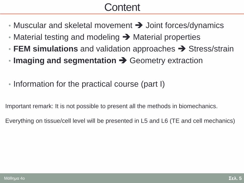
Content

• Muscular and skeletal movement Joint forces/dynamics

• Material testing and modeling Material properties

• FEM simulations and validation approaches Stress/strain

• Imaging and segmentation Geometry extraction

• Information for the practical course (part I)

Σελ. 5

Important remark: It is not possible to present all the methods in biomechanics.

Everything on tissue/cell level will be presented in L5 and L6 (TE and cell mechanics)

Μάθημα 4ο

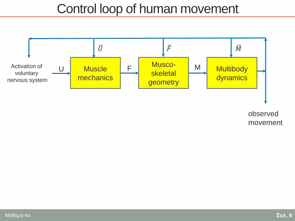
Control loop of human movement

Σελ. 6

observed

movement

Muscle

mechanics

Musco-

skeletal

geometry

Multibody

dynamics

U F M

𝑀 𝐹 𝑈

Activation of

voluntary

nervous system

Μάθημα 4ο

Muscle mechanics (Hill-Model)

Σελ. 7

ElectromyographySignal processing (Filtering, FFT,

Thresholding..)

Which muscle is activated?

At what time point?

What is the force F?

Μάθημα 4ο

EMG example

Σελ. 8

Healthy Spasticity

In pathological scenarios (spasticity) the interplay

between agonists and antagonists is deteriorated.

Uncoordinated movement and high joint loads!

EMG + gait monitoring can be used

for diagnosis and therapy

Μάθημα 4ο

Musco-skeletal geometry

Σελ. 9

Lever arm

Force

Momentum

Starting points and end points of muscles

Bone size and orientation

Imaging (difficult), anatomical knowledge, generic models

Momentum

Only when studying individual joints

Μάθημα 4ο

Measurement of forces

Σελ. 10

In vivo force measurement is invasive Instrumented implants or pressure

indicating films

Μάθημα 4ο

Multi-body dynamics

Σελ. 11

Movement

of the entire body

Movement

and moments

at joints

Muscle forces

Activation profiles

Inverse problem fitting to EMG data and movement adaptation until EMGexp=EMGsim

Μάθημα 4ο

Complex model under-constrained optimization problem

Σελ. 12

Complex models (which are not necessarily better than simpler models) require

further constraints to allow a unique solution.

Energy minimization of muscle activity Joint loading minimization

Movement duration minimizationVALIDATION

Μάθημα 4ο

3D movement tracking

Σελ. 13

Validation of simulations

Providing boundary conditions

for simulations

In vivo studies (pathologies,

rehabilitation, device design)

Connection

to other measurements (EMG)

Μάθημα 4ο

Summary - Gait

Σελ. 14

Muscle

mechanics

Musco-

skeletal

geometry

Multibody

dynamics

Only the combination of experiment and simulation together with cross-validation

can deliver a reliable and useful model!

Μάθημα 4ο

Examples : Pathologies - Stroke

Σελ. 15

https://www.youtube.com/watch?v=ecWBdL6-y6Q

Μάθημα 4ο

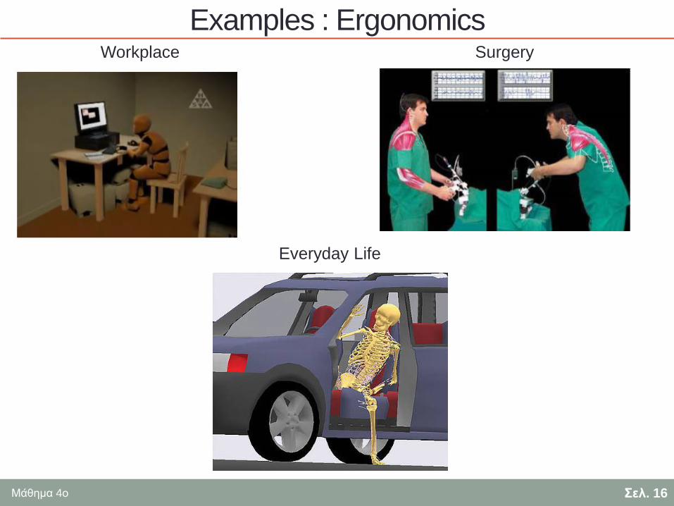
Examples : Ergonomics

Σελ. 16

Workplace Surgery

Everyday Life

Μάθημα 4ο

Examples: Sport biomechanics

Σελ. 17

https://www.youtube.com/watch?v=7u2Rqm5fXus

Μάθημα 4ο

Questions?

Σελ. 18

Μάθημα 4ο

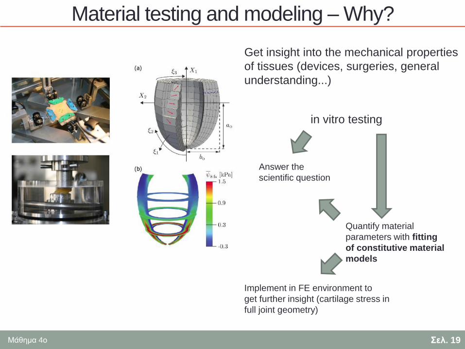
Material testing and modeling – Why?

Σελ. 19

Get insight into the mechanical properties

of tissues (devices, surgeries, general

understanding...)

in vitro testing

Answer the

scientific question

Quantify material

parameters with fitting

of constitutive material

models

Implement in FE environment to

get further insight (cartilage stress in

full joint geometry)

Μάθημα 4ο

Properties of biological tissues

L3: Biological tissues are

• non-linear elastic (hyperelastic)

• stiffness depends on loading direction (anisotropic)

• stiffness depends on loading velocity (viscoelastic)

• creep/relaxation/hysteresis (viscoelastic)

In special cases, e.g. cartilage

• fluid embedded in solid matrix (bi or tri-phasic)

• Long-term observation includes remodeling

Σελ. 20

Μάθημα 4ο

Hyperelasticity

Σελ. 21

Tensile test of carotid artery

Non-linear stress-strain behavior of an elastic material (no plastic deformation)

Described by a strain energy density function

First developed for elastomers and polymers

Compression test of cartilage

Μάθημα 4ο

Anisotropy

Σελ. 22

Compression tests of bone

Stress-strain behavior depends on loading direction (anisotropy)

Orthotropy (3 different Young’s moduli) and transversal isotropy (2 different

Young’s moduli) are the most common forms of directed anisotropy

Loading and remodeling defines material directions (Wolff’s Law!)

Μάθημα 4ο

Identification of material parameters from in vitro data

Σελ. 23

Decided what we want to know : anisotropic properties (E1 and E2) of tissue

Did our experiments : tension/compression tests is axial direction 1 and 2

Choose a mathematical representation of our material model

Fit our material model to the data to derive the Young’s modulus

Μάθημα 4ο

Continuum mechanics of soft tissues

Σελ. 24

Remark: Normally some “new” mathematics needed. Tensor algebra and analysis

(E.g. Book by Prof. Itskov from RWTH Aachen University) for the extremely interested

student. As well as books by G.A. Holzapfel and G.W. Ogden.

In application the following is done by software (Abaqus FEM). What

follows is a very short presentation of the steps from material model choice to

parameter identification.

Μάθημα 4ο

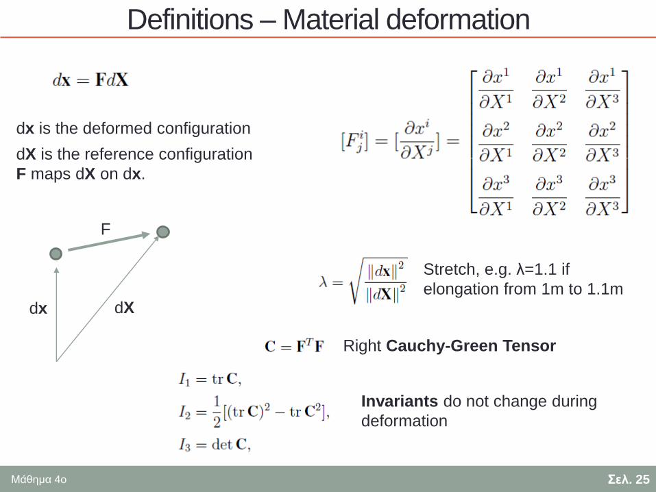
Definitions – Material deformation

Σελ. 25

dx is the deformed configuration

dX is the reference configuration

F maps dX on dx.

F

dx dX

Stretch, e.g. λ=1.1 if

elongation from 1m to 1.1m

Right Cauchy-Green Tensor

Invariants do not change during

deformation

Μάθημα 4ο

Material deformation summary

Cauchy-Green tensor C describes material deformation

For every state of the material the Cauchy-Green tensor can

be computed.

Invariants are calculated from C. Will be important in the next

steps

Material strain (ε) is expressed with Green-Lagrange Strain

Tensor E.

Σελ. 26

Identity tensor

Μάθημα 4ο

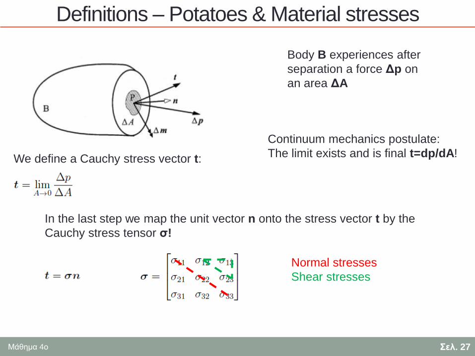
Definitions – Potatoes & Material stresses

Σελ. 27

Body B experiences after

separation a force Δp on

an area ΔA

We define a Cauchy stress vector t:

Continuum mechanics postulate:

The limit exists and is final t=dp/dA!

In the last step we map the unit vector n onto the stress vector t by the

Cauchy stress tensor σ!

Normal stresses

Shear stresses

Μάθημα 4ο

Definitions II – Stress Tensors

Σελ. 28

Infinitesimal force on infinitesimal deformed area

First Piola Kirchhoff stress tensor relates the

stress to the initial configuration

J= det C = relative volume change J=1 if incompressible material

Second Piola Kirchhoff stress tensor relates the

stress to the actual configuration

Generalized Hooke’s Law

Derivation of Stress Tensor S w.r.t. Strain Tensor E

Compliance Tensor C (4. order tensor) includes material properties (E,G,ν)

Μάθημα 4ο

Summary Continuum Mechanics Crash Course

All deformation can be expressed by Cauchy-Green tensor C

All stresses can be expressed by Piola-Kirchhoff tensor P or

S, respectively

Stress and strain are connected with Hooke’s Law via

Σελ. 29

Inverse of compliance tensor for an isotropic material

Μάθημα 4ο

Hyperelastic material defined by strain energy function

Σελ. 30

Strain energy function defined by invariants (deformation)

This is the constitutive model provided for fitting.

Stress calculated from strain energy function connection

between material model, stress and strain!

Neo-Hookean model (isotropic)

Material modeling procedure:

1. Do material tests

2. Calculate C from the deformation

3. Define Pexp or Sexp from force measurements

4. Derive Pmod or Smod from ψ

5. Parameter fitting Pexp/Pmod or Sexp/Smod

6. Calculate E/G/ν from fitted model

Μάθημα 4ο

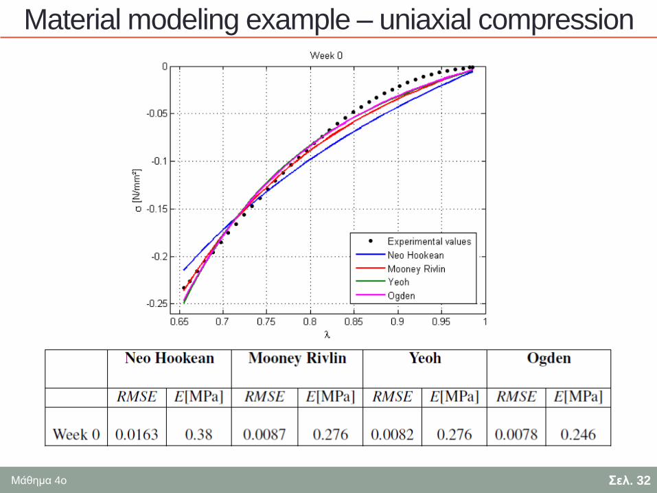
Material modeling example – uniaxial compression

Σελ. 31

incompressibility

+

unconfined deformation

Invariants depend on the deformation

conditions

Stress in the first direction (output of compression tester)

Μάθημα 4ο

Material modeling example – uniaxial compression

Σελ. 32

Μάθημα 4ο

Strain energy functions - This is what you select in FEM

Σελ. 33

Holzapfel Model

Isotropic matrixFiber-reinforcement,

I4 depends on fiber direction anisotropy

Very popular model for biological tissues. Included in common FE solvers

like ABAQUS, ANSYS, Comsol...

Ogden ModelMooney Rivlin Model

Μάθημα 4ο

Viscoelasticity

Σελ. 34

Energy dissipation during material deformation

Time-dependent stress-strain response

Included as an additional term in material models

CreepRelaxation

Hysteresis

Velocity-dependence

Μάθημα 4ο

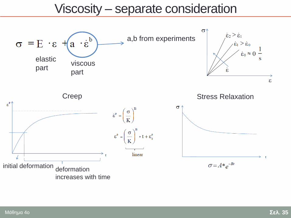
Viscosity – separate consideration

Σελ. 35

a,b from experiments

elastic

partviscous

part

initial deformationdeformation

increases with time

Creep Stress Relaxation

Μάθημα 4ο

Poroviscoelasticity of cartilage

Σελ. 36

Fluid phase embedded in solid phase

Fluid flow through media is governed by

hydraulic permeability k

porosity Φ

Both depend on the deformation of the tissue

FE analysis (inverse simulate and find material

properties by fitting deformation curve(exp) to simulation)

Μάθημα 4ο

Example – FE simulations of a bi-phasic model

Σελ. 37

Qeng et al.2013

Μάθημα 4ο

Include remodeling in material model (E(t))

Σελ. 38

Knee joint from imaging data +

Gait loading (gait biomechanics)

Fibril-reinforced cartilage material

model with fibril stiffness depending on stress

Cartilage degeneration from FEM stress

Mononen et al. 2016

Hyperelastic matrix (Neo-Hookean) +

pores +

viscoelastic fibrils(layer-dependent orientation)

Μάθημα 4ο

Model validation with clinical study

Σελ. 39

Comparison with clinical trial data of 44 patients with a 4-year follow up

Mononen et al. 2016

Μάθημα 4ο

Summary material modeling

Material models to quantify material properties and further

investigations in FEM simulations

Choose what do you want to investigate (anisotropy, cyclic

loading, creep, material failure...) do experiments (uniaxial,

biaxial, shear etc.) choose material model and fit

parameters

Many factors play a role! It is difficult (not impossible) to

include all of them in material model. E.g. hyperelasticity,

anisotropy, remodeling, viscoelasticity, poroelasticity etc.

Implement model and validate with further experiments...

Σελ. 40

Μάθημα 4ο

Questions?

Σελ. 41

Μάθημα 4ο

FEM

Σελ. 42

Μάθημα 4ο

FEM Idea

Σελ. 43

Approach: Divide a complex geometry into a mesh of simple interconnected elements

Calculation of deformations in each cell with approximate solutions

Determination of total deformation after consideration of each cell deformation

and existing interconnections

Μάθημα 4ο

FEM simple example

Σελ. 44

Force at node 1 is spring constant 1 multiplied by the absolute length change

of the spring.

F1=c1*u1-c1*u2

Μάθημα 4ο

Stiffness matrix and boundary conditions

Σελ. 45

Stiffness matrix

Boundary conditions (no movement of node 1, no spring 3) simplify the matrix

Μάθημα 4ο

Application for real cases

Σελ. 46

Sparse (many entries are 0)

matrix compute the inverse

with numerical algorithms (PDEs)

Our elements are more complicated than simple mass-spring systems

shear deformations, material models (viscoelasticity, big deformations etc...)

take approximate solutions of each node deformation (next slide)

Μάθημα 4ο

Approximation function for linear beam

Σελ. 47

On the beam l acts a distributed load q. The deformation is approximated with

the linear function w.

After the approximation we have a system with a finite number of degrees of

freedom (DOFs).

The system is solved (minimization of internal energy difference) numerically.

Μάθημα 4ο

Summary FEM Theory

Σελ. 48

We discretize the geometry.

Express the force/deformation relationship with a system of PDEs.

This system has a number DOFs depending on the discretization approach.

System solution (matrix inversion) is done numerically.

We stop when the difference in our variables

(internal energy U, force F, deformation u) are below a convergence target.

More complicated cases need consideration of other factors (contact and shock, big

deformations and remeshing, non-linear materials and numerical stability, fluid and

solid interactions...)

The FEM method is well established (1950s-60s in the automotive and aerospace

industry) and reliable commercial and open source solvers exist which allow

user-friendly solutions of nowadays problems.

Μάθημα 4ο

FEM with focus on application

In the following the usual steps in a FE simulation are

presented.

Focus is put on the reasoning and necessity of each step as

well as possible pitfalls and problems that might come up

during a simulation.

Commercial programs provide huge documentations with

theory and application for every specific problem. Tutorials

and workshops can be acquired from companies’ websites.

The following should be considered as a best practice

routine. What should be the mindset for a successful

simulation.

Σελ. 49

Μάθημα 4ο

Step 0: What’s your problem?

Σελ. 50

The research question defines the purpose and “style” of our simulation.

Parameterized design study

many simulations

high stability

low numerical costs

One specific case for mechanical insight

careful geometry extraction

realistic material modeling

high numerical costs

Marangalou 2012Clinical study

Many uncertainties

Method development

A lot of numerics

Μάθημα 4ο

Step 1: Geometry creation/extraction

Especially after segmentation from imaging data the geometry

has to be smoothed and/or trimmed accordingly

Σελ. 51

Liao et al. 2016

Μάθημα 4ο

Step 2: Meshing

Decide on the mesh element type (free or mapped)

Σελ. 52

For complex geometries

often unstructured (free) tetrahedral meshes.

Mesh size and numerical costs

Element deformation (1 bad element can

destroy entire simulation)

Unstructured is much easier

Μάθημα 4ο

Step 3: Boundary conditions

Σελ. 53

Force/pressure/momentum/displacement

Locating/floating bearing

(Rotational) symmetry when possible.

Contact!

Contact pairs, force/deformation translation

and penetration are often the reason for

instabilities/slow simulations/problems.

Gap closure for better stability

Μάθημα 4ο

Step 4: Material models

Biological materials are very complicated. Material description and

modeling is still ongoing. Based on the research question you should

choose the phenomena you want to represent.

Especially non-linearity and combinations of materials with different

properties (layers) can cause problems Better start simple, then switch

to complicated material models if everything else works!

Σελ. 54

Material model choice and parameter fitting (like in lecture)

Μάθημα 4ο

Step 5: Choice of solver

Σελ. 55

Stable solvers for various problems (implicit/explicit)

Time step size/duration of simulation

Convergence target

Under-relaxation factors (increased stability, increased

calculation time)

... a big world

Μάθημα 4ο

Step 6: Independence studies

Our solution is an approximation of the initial geometry.

Guarantee that the solution does not depend on intrinsic

factors like timestep, solver settings, b.c. and mesh size

Σελ. 56

Μάθημα 4ο

Questions?

Σελ. 57

Μάθημα 4ο

Imaging

Visual representation of human body parts or functions of

organs and tissues

Analysis, Diagnosis, Intervention

Most of the methods are non-invasive

Σελ. 58

Clinician

Researcher

Engineer

Μάθημα 4ο

Imaging

Σελ. 59

Echocardiography

CT

fMRI

PET

MRI

Angiography

X-ray

Fluorescent imaging

Μάθημα 4ο

CT (Computed tomography) working principle

Σελ. 60

Many X-ray scans taken from different angles to produce

tomographic (sectional) images of 3D body

Different tissues absorb x-rays in a different way grayscale values

Many applications: hard tissues, tumors, cardiovascular..

Around 1-5mm slice thickness. µCT much smaller, just for research

Patient objected to radiation. 1-4x yearly radiation exposure

Benefit often outweighs

Μάθημα 4ο

MRI (Magnet resonance imaging) working principle

Σελ. 61

Hydrogen atoms in tissues absorb and emit

energy in an external magnetic field

Different tissues react differently, water and fat locations grayscale values

Many applications: soft tissues (muscles, ligaments, cartilage)

hard tissues, tumors, cardiovascular..

Around 0.2-5mm slice thickness. 4D MRI for time-dependent scans!

No radiation. Magnetic field not able to use for every patient. May be experienced

as claustrophobic. Should not be overused Often as a 2. means of diagnosis

Μάθημα 4ο

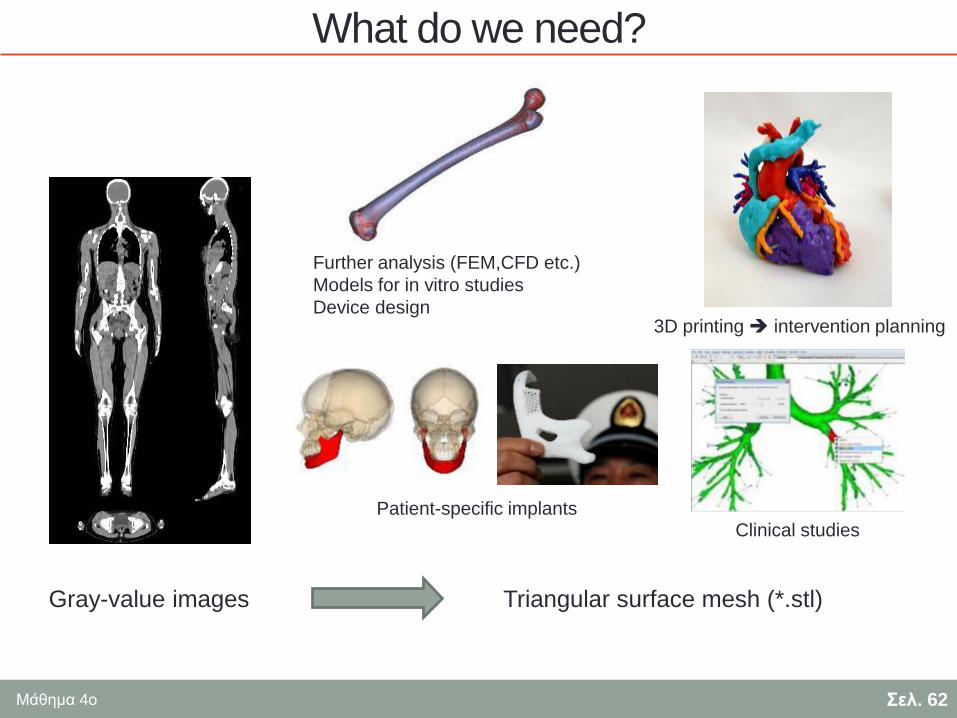
What do we need?

Σελ. 62

Gray-value images

Further analysis (FEM,CFD etc.)

Models for in vitro studies

Device design3D printing intervention planning

Patient-specific implantsClinical studies

Triangular surface mesh (*.stl)

Μάθημα 4ο

Segmentation – preamble

Segmentation is the partitioning of a digital image into multiple

segments of interest.

2D slices 3D surface

Theory of segmentation will not be covered in the following

slides. In general there are many open-source and

commercial programs which allow an efficient segmentation

without knowledge of the background.

Σελ. 63

Μάθημα 4ο

Image pre-processing - Thresholding

Σελ. 64

Different tissues produce different grayscale values. E.g. Bone vs. soft tissues.

Increasing the intensity/contrast of the respective intensity values helps

to distinguish the tissues. Some tissue thresholds

are already stored inside the software.

Μάθημα 4ο

Manual segmentation

Σελ. 65

Very straightforward procedure. Marking the regions of interest (red paint) on

each slice and creating 3D model them.

Μάθημα 4ο

Semi-automatic segmentation

Σελ. 66

Basic idea: Place seeds/sources at the parts of interest. Then let the regions grow until

the boundary of the part of interest is reached.

However mistakes like this can appear

Pre-processing and modification of

segmentation parameters based on application

case is important. Also the knowledge of the

geometry!!!

Μάθημα 4ο

Semi-automatic segmentation

Σελ. 67

Μάθημα 4ο

Semi-automatic segmentation

Σελ. 68

Careful pre-processing is important!

After model creation post-processing (smoothing, cut-planes etc.)

Μάθημα 4ο

Automatic segmentation

Very active area of research and development

Artificial intelligence and machine learning are supposed

to overcome the limitations of current algorithms and

problems like inter-observatory and intra-observatory

variations

Huge medical impact and databases existing (hospitals)

Σελ. 69

Cancer Cardiovascular Orthopedic

Μάθημα 4ο

Questions?

Σελ. 70

Μάθημα 4ο

Summary

Investigations in biomechanics include various fields such as:

Signal processing, image analysis, general mechanics, multi-body

dynamics, heat and mass transfer, fluid dynamics, statistics etc.

There are no biological constants, every parameter experiences huge

variations (stiffness, size, weight...) and changes over time (remodeling).

The engineering approach of understanding and modifying complex

systems reaches its limits however might be still better than the clinical

‘trial-and-error’ approach.

Σελ. 71

Μάθημα 4ο

Sources

https://spinevuetx.com/wp-content/uploads/2017/08/miss-vs-trad.jpg

https://image.slidesharecdn.com/emgelectrodeplacement-140527040535-phpapp01/95/emg-13-638.jpg?cb=1401263682

Biomechanik des Bewegungs- und Stützapparates, Radermacher, RWTH Aachen

www.youtube.com

en.wikipedia.org

http://www.medkiozk.com/mdkzk14/wp-content/uploads/2013/07/image006.jpg

https://www.intechopen.com/source/html/18159/media/image18.png

http://biomechanical.asmedigitalcollection.asme.org/data/journals/jbendy/930653/bio_136_10_101004_f004.png

https://www.biomech.tugraz.at/index.php/research#human%20myocardium

Meng, Qingen, et al. "Comparison between FEBio and Abaqus for biphasic contact problems." Proceedings of the Institution of Mechanical Engineers,

Part H: Journal of Engineering in Medicine 227.9 (2013): 1009-1019.

Mononen, Mika E., et al. "A novel method to simulate the progression of collagen degeneration of cartilage in the knee: data from the osteoarthritis

initiative." Scientific reports 6 (2016).

http://www.iaas.uni-stuttgart.de/forschung/projects/simtech/img/bone2.png

Marangalou, Javad Hazrati, Keita Ito, and Bert van Rietbergen. "A new approach to determine the accuracy of morphology–elasticity relationships in

continuum FE analyses of human proximal femur." Journal of biomechanics 45.16 (2012): 2884-2892.

Liao, Sam, et al. "Numerical prediction of thrombus risk in an anatomically dilated left ventricle: the effect of inflow cannula designs." Biomedical

engineering online 15.2 (2016): 136.

https://images.radiopaedia.org/images/17022935/5176e6a2ad4a6418e8b38792a5aedf_big_gallery.jpeg

https://www.researchgate.net/publication/261140200/figure/fig2/AS:214304323313668@1428105540826/CT-scan-documenting-sub-capital-fracture-of-

the-femur.png

http://calrads.org/wp-content/uploads/2016/09/x-ray.jpg

https://textimgs.s3.amazonaws.com/boundless-anatomy-and-physiology/human-anatomy-planes.svg

https://www.3ders.org/images/titanium-lower-jaw-china-2.jpg

Σελ. 72