Embed Size (px)
Citation preview
Biometric quality and its impact on template
ageing in a longitudinal �ngerprint study
by
Henry John Harvey
A thesis submitted to the Faculty of Graduate Studies and Research
in partial ful�llment of the requirements for the degree of
Doctor of Philosophyin
Electrical and Computer Engineering
Carleton University
Ottawa, Ontario, Canada, K1S 5B6
©2019 Henry John Harvey

Abstract
Biometrics are increasingly deployed in domains ranging from social media authenti-
cation right up to border control. An important operational requirement for biometric
systems is the supposed uniqueness and permanence of biometric records: physiolog-
ical changes occurring between enrolment and veri�cation are referred to as template
ageing, and increase the likelihood of a misidenti�cation. Its magnitude is hard to
estimate, and the factors a�ecting it are relatively little studied.
This work proposes a measure of template ageing, called biometric permanence,
and develops a methodology to estimate it in the presence of confounding factors.
The measure is applied to a database of �ngerprints obtained over a seven year pe-
riod, using bootstrap resampling to obtain con�dence intervals for the estimates of
e�ect size. Fingerprint quality metrics are evaluated in terms of their ability to pre-
dict classi�cation performance, and the subject-dependence of �ngerprint quality is
explored using the ideas of a �biometric menagerie�. Statistically signi�cant demo-
graphic factors underlying biometric quality and template ageing are highlighted and
discussed.
The results of this work may have implications for the procurement and adminis-
tration of biometric systems: for example, in ensuring consistent performance across
a broad population demographic, and in the choice of credential lifetime and re-
enrolment policy.

Dedication
For REE
ii
Acknowledgements
I would like to thank David Dawson for coordinating and overseeing the data col-
lection, and Bion Biometrics, Inc. for making available the ISBIT database and
software.
The experimental phases of this work were supported in part by the Natural
Sciences and Engineering Research Council (NSERC), grant number CRD 428240-
11.
I would like to thank Dr. Andy Adler, my supervisor, for encouraging me to
undertake this work and for his continued support; and Dr. John Campbell for his
many helpful suggestions.
iii
Contents
1 Introduction 1
1.1 Problem statement . . . . . . . . . . . . . . . . . . . . . . . . . . . . 1
1.2 Goals . . . . . . . . . . . . . . . . . . . . . . . . . . . . . . . . . . . . 5
1.3 Contributions . . . . . . . . . . . . . . . . . . . . . . . . . . . . . . . 5
1.3.1 Methodology for estimating biometric permanence . . . . . . . 5
1.3.2 Observation and quanti�cation of template ageing . . . . . . . 6
1.3.3 Investigation of the e�ect of biometric data quality on classi�-
cation performance . . . . . . . . . . . . . . . . . . . . . . . . 6
1.3.4 Observation and demographics of a biometric menagerie . . . 7
1.3.5 Outline for a biometric channel model . . . . . . . . . . . . . 7
1.4 Publications . . . . . . . . . . . . . . . . . . . . . . . . . . . . . . . . 7
2 Background and literature review 9
2.1 History and early application of biometrics . . . . . . . . . . . . . . . 9
2.2 Modern biometrics . . . . . . . . . . . . . . . . . . . . . . . . . . . . 10
2.2.1 Renewable biometric references . . . . . . . . . . . . . . . . . 11
2.2.2 Forensic applications . . . . . . . . . . . . . . . . . . . . . . . 11
2.3 Biometric template ageing . . . . . . . . . . . . . . . . . . . . . . . . 12
2.4 De�nition and evaluation of biometric data quality . . . . . . . . . . 15
2.5 The biometric menagerie . . . . . . . . . . . . . . . . . . . . . . . . . 18
iv
CONTENTS v
2.6 Relationship between template ageing, quality, and demographics . . 19
2.7 Open questions . . . . . . . . . . . . . . . . . . . . . . . . . . . . . . 20
3 The �Norwood� dataset 21
3.1 History and demographics . . . . . . . . . . . . . . . . . . . . . . . . 21
3.2 Data collection protocol . . . . . . . . . . . . . . . . . . . . . . . . . 24
3.2.1 Carleton modi�cations to the software and protocol . . . . . . 26
3.3 Study terminology and notation . . . . . . . . . . . . . . . . . . . . . 26
3.4 Biometric record storage and retrieval . . . . . . . . . . . . . . . . . . 27
3.4.1 Database structure . . . . . . . . . . . . . . . . . . . . . . . . 27
3.4.2 Binary Biometric Information Record (BIR) structure . . . . . 28
4 Biometric permanence: de�nition and robust calculation 30
4.1 Introduction . . . . . . . . . . . . . . . . . . . . . . . . . . . . . . . . 30
4.2 Methodology . . . . . . . . . . . . . . . . . . . . . . . . . . . . . . . 31
4.2.1 De�nition . . . . . . . . . . . . . . . . . . . . . . . . . . . . . 32
4.2.2 Robust calculation . . . . . . . . . . . . . . . . . . . . . . . . 34
4.2.3 Visit aggregation . . . . . . . . . . . . . . . . . . . . . . . . . 37
4.3 Simulation . . . . . . . . . . . . . . . . . . . . . . . . . . . . . . . . . 39
4.3.1 Simulation of a single sequence of visits . . . . . . . . . . . . . 40
4.3.2 Simulation of an ensemble of visit sequences . . . . . . . . . . 42
4.4 Discussion . . . . . . . . . . . . . . . . . . . . . . . . . . . . . . . . . 45
5 Characterization of biometric template ageing in a multi-year, multi-
vendor longitudinal �ngerprint matching study 46
5.1 Methodology . . . . . . . . . . . . . . . . . . . . . . . . . . . . . . . 47
5.2 Results . . . . . . . . . . . . . . . . . . . . . . . . . . . . . . . . . . . 50
5.3 Discussion . . . . . . . . . . . . . . . . . . . . . . . . . . . . . . . . . 61
5.3.1 Time symmetry of the match scores . . . . . . . . . . . . . . . 62

CONTENTS vi
5.3.2 Constancy of the imposter distributions . . . . . . . . . . . . . 63
5.4 Conclusion . . . . . . . . . . . . . . . . . . . . . . . . . . . . . . . . . 68
6 Biometric quality and classi�cation performance 69
6.1 History and application of the NFIQ measures . . . . . . . . . . . . . 69
6.1.1 NFIQ-1 . . . . . . . . . . . . . . . . . . . . . . . . . . . . . . 69
6.1.2 NFIQ-2 . . . . . . . . . . . . . . . . . . . . . . . . . . . . . . 70
6.1.3 Vendor quality metrics . . . . . . . . . . . . . . . . . . . . . . 70
6.2 Generation of the NFIQ scores . . . . . . . . . . . . . . . . . . . . . . 71
6.3 Extraction of vendor quality scores . . . . . . . . . . . . . . . . . . . 72
6.4 Comparisons of NFIQ1, NFIQ2, and vendor quality . . . . . . . . . . 72
6.5 E�ect of biometric quality on match score . . . . . . . . . . . . . . . 77
6.6 E�ect of biometric quality on classi�cation accuracy . . . . . . . . . . 90
6.7 Discussion . . . . . . . . . . . . . . . . . . . . . . . . . . . . . . . . . 100
7 Identi�cation and demographics of a biometric menagerie, and its
e�ect on classi�cation performance and template ageing 101
7.1 Revisiting Doddington's zoo . . . . . . . . . . . . . . . . . . . . . . . 102
7.1.1 Identi�cation of a common Goat subset . . . . . . . . . . . . . 102
7.1.2 Demographics of the Goat subset . . . . . . . . . . . . . . . . 105
7.1.3 NFIQ quality of the Goat subset . . . . . . . . . . . . . . . . 114
7.2 Wolves, Lambs and Sheep . . . . . . . . . . . . . . . . . . . . . . . . 121
7.2.1 Demographics of the Lamb and Wolf subsets . . . . . . . . . . 122
7.2.2 NFIQ quality of the Lamb and Wolf subsets . . . . . . . . . . 129
7.3 E�ect of Goats on biometric permanence . . . . . . . . . . . . . . . . 133
7.4 Discussion . . . . . . . . . . . . . . . . . . . . . . . . . . . . . . . . . 142
8 Discussion 143
8.1 Estimation of biometric permanence . . . . . . . . . . . . . . . . . . . 143
CONTENTS vii
8.1.1 Motivation for the biometric permanence metric . . . . . . . . 143
8.1.2 Assumptions and limitations . . . . . . . . . . . . . . . . . . . 144
8.1.3 Illustrative application of the metric . . . . . . . . . . . . . . 145
8.2 Validation of NFIQ quality metrics . . . . . . . . . . . . . . . . . . . 146
8.3 Presence of a biometric menagerie . . . . . . . . . . . . . . . . . . . . 146
8.4 Biometrics as a communication channel . . . . . . . . . . . . . . . . . 147
8.4.1 Biometric rate and capacity . . . . . . . . . . . . . . . . . . . 148
8.4.2 Biometric �good codes� . . . . . . . . . . . . . . . . . . . . . . 149
8.5 Information-theoretic interpretation of template ageing . . . . . . . . 149
8.6 Suggestions for future work . . . . . . . . . . . . . . . . . . . . . . . 152
A Sample MSSQL database queries 154
B Unpacking the BioAPI Biometric Information Record 156
C Bootstrap resampled con�dence interval (CI) for PB 159
D A note on the Rayleigh synthetic match score distributions 163
D.1 Tail integral for the FMR . . . . . . . . . . . . . . . . . . . . . . . . 164
D.2 Tail integral for the FNMR . . . . . . . . . . . . . . . . . . . . . . . 166
List of Figures
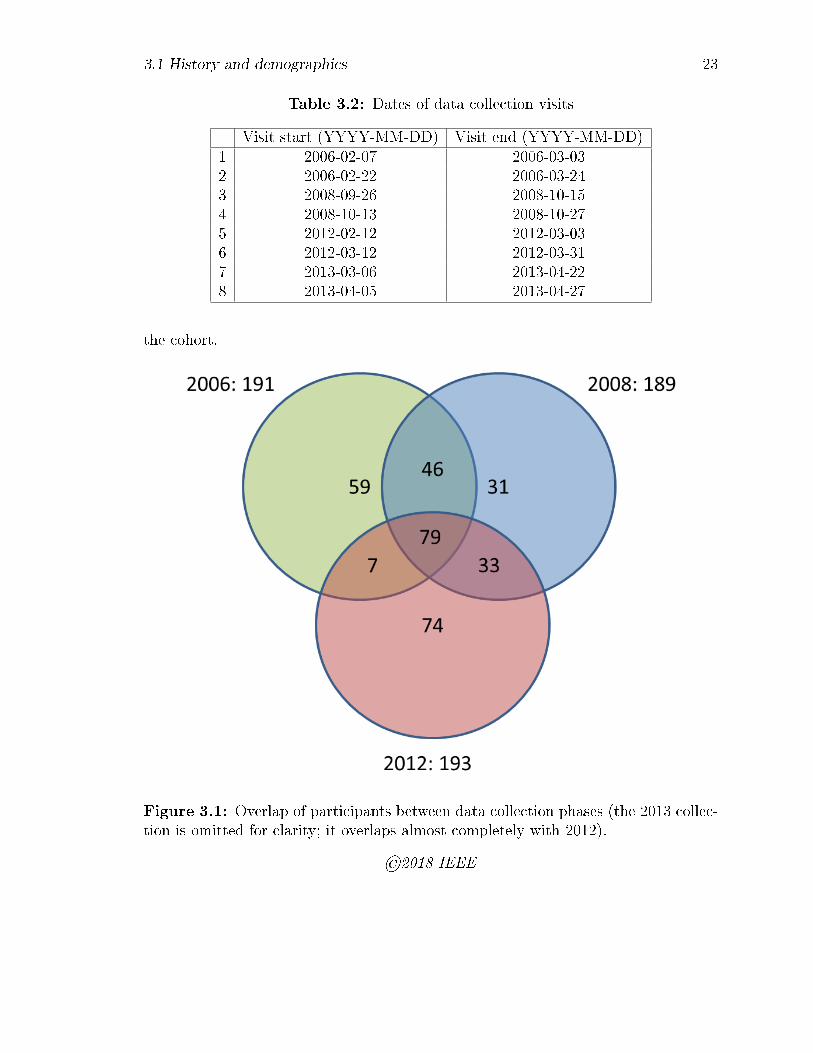
3.1 Overlap of participants between data collection phases (the 2013 col-
lection is omitted for clarity; it overlaps almost completely with 2012). 23
3.2 The author's own left and right index �ngers, annotated with the minu-
tiae obtained during enrolment on Device L . . . . . . . . . . . . . . . 29
4.1 Overview of the method: (a) empirical match score distributions imme-
diately after enrolment (top), and after some time interval (bottom);
(b) change in classi�cation accuracy represented on a decision error
trade-o� (DET) curve: arrows indicate the directions of increasing se-
curity and convenience; (c) permanence PB derived from the change in
FNMR at �xed FMR according to Eq. 4.1. . . . . . . . . . . . . . . . 33
4.2 Matrix of visits for a single subject over the protocol. Each row and col-
umn represents a visit (with enrol, Em and veri�cation, Vn records). In
our testing protocol, each round of testing has a pair of visits separated
by two weeks. The upper triangle represents match scores �forward in
time� (Em vs. Vn, m < n), while the lower represents the corresponding
match scores �backward in time� (Em vs. Vn, m > jn). Match scores
on the diagonal are from the same visit (i.e. ∆t = 0). . . . . . . . . . 38
viii
LIST OF FIGURES ix
4.3 Simulation of the e�ect of visit biases. Top row: noise only; middle
row: noise and enrol visit biases; bottom row: noise, enrol and verify
bias. The case of noise plus verify bias only is omitted for brevity. Red
stars are the reference method of Section 4.2.1 while blue circles are
our matched delta method of Section 4.2.2. The black curve is derived
from the analytical tail integrals of Eq. 4.7. . . . . . . . . . . . . . . 43
4.4 Di�erence (±SD) between the reference measure Section 4.2.1 and the
matched delta method of Section 4.2.2 as the size of the experiment
ensemble is increased. . . . . . . . . . . . . . . . . . . . . . . . . . . 44
5.1 Computation time of the bootstrap CI versus dataset size, nTot =
nG + nI for the original procedure . . . . . . . . . . . . . . . . . . . . 48
5.2 A shift in the mean imposter score results in a shift in the estimated
decision threshold θ0 for a speci�ed FMR (red area) � and a corre-
sponding change in the achievable TMR (blue area) for the shifted
genuine scores. . . . . . . . . . . . . . . . . . . . . . . . . . . . . . . 50
5.3 Match score distributions, DET, and PB: DeviceB (optical) . . . . . 52
5.4 Match score distributions, DET, and PB: DeviceC (optical) . . . . . 53
5.5 Match score distributions, DET, and PB: DeviceD (optical) . . . . . 54
5.6 Match score distributions, DET, and PB: Device F (optical) . . . . . 55
5.7 Match score distributions, DET, and PB: DeviceG (optical) . . . . . 56
5.8 Match score distributions, DET, and PB: DeviceH (optical) . . . . . 57
5.9 Match score distributions, DET, and PB: Device J (optical) . . . . . . 58
5.10 Match score distributions, DET, and PB: DeviceK (optical) . . . . . 59
5.11 Match score distributions, DET, and PB: Device L (capacitive) . . . . 60
LIST OF FIGURES x
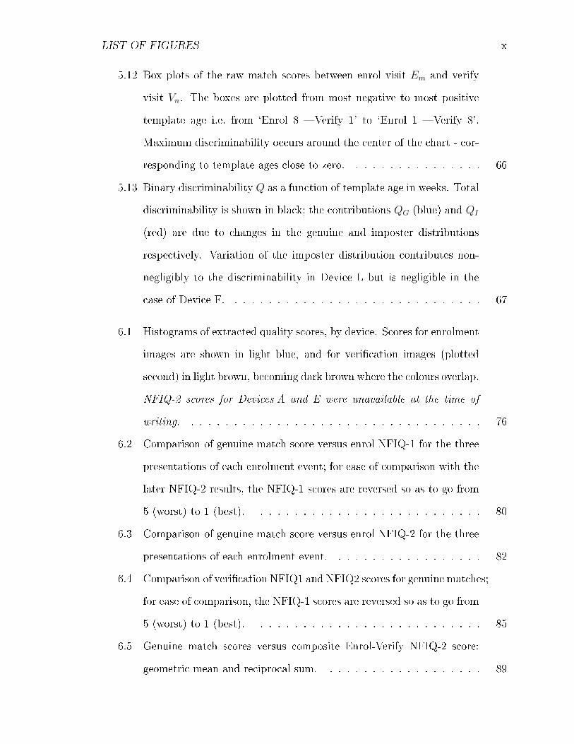
5.12 Box plots of the raw match scores between enrol visit Em and verify
visit Vn. The boxes are plotted from most negative to most positive
template age i.e. from `Enrol 8 � Verify 1' to `Enrol 1 � Verify 8'.
Maximum discriminability occurs around the center of the chart - cor-
responding to template ages close to zero. . . . . . . . . . . . . . . . 66
5.13 Binary discriminability Q as a function of template age in weeks. Total
discriminability is shown in black; the contributions QG (blue) and QI
(red) are due to changes in the genuine and imposter distributions
respectively. Variation of the imposter distribution contributes non-
negligibly to the discriminability in Device L but is negligible in the
case of Device F. . . . . . . . . . . . . . . . . . . . . . . . . . . . . . 67
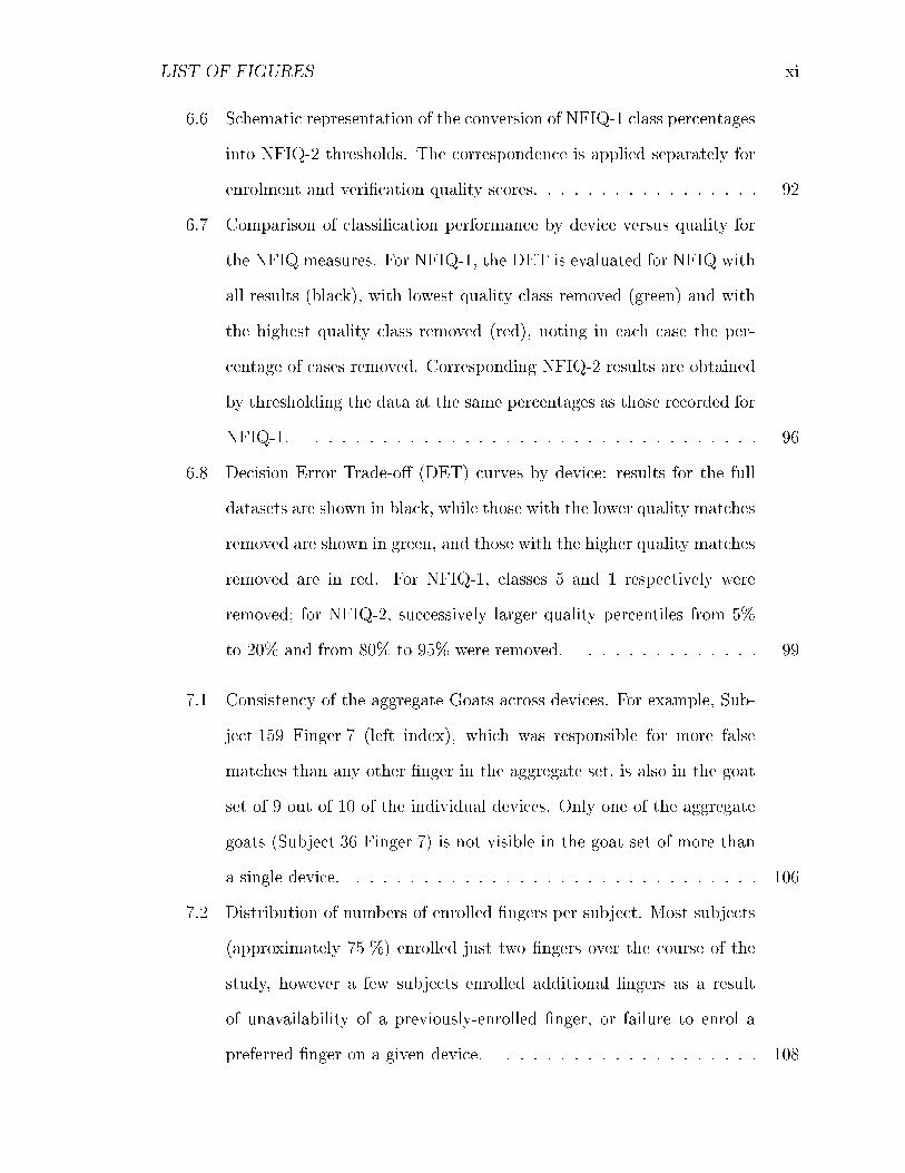
6.1 Histograms of extracted quality scores, by device. Scores for enrolment
images are shown in light blue, and for veri�cation images (plotted
second) in light brown, becoming dark brown where the colours overlap.
NFIQ-2 scores for Devices A and E were unavailable at the time of
writing. . . . . . . . . . . . . . . . . . . . . . . . . . . . . . . . . . . 76
6.2 Comparison of genuine match score versus enrol NFIQ-1 for the three
presentations of each enrolment event; for ease of comparison with the
later NFIQ-2 results, the NFIQ-1 scores are reversed so as to go from
5 (worst) to 1 (best). . . . . . . . . . . . . . . . . . . . . . . . . . . 80
6.3 Comparison of genuine match score versus enrol NFIQ-2 for the three
presentations of each enrolment event. . . . . . . . . . . . . . . . . . 82
6.4 Comparison of veri�cation NFIQ1 and NFIQ2 scores for genuine matches;
for ease of comparison, the NFIQ-1 scores are reversed so as to go from
5 (worst) to 1 (best). . . . . . . . . . . . . . . . . . . . . . . . . . . 85
6.5 Genuine match scores versus composite Enrol-Verify NFIQ-2 score:
geometric mean and reciprocal sum. . . . . . . . . . . . . . . . . . . 89
LIST OF FIGURES xi
6.6 Schematic representation of the conversion of NFIQ-1 class percentages
into NFIQ-2 thresholds. The correspondence is applied separately for
enrolment and veri�cation quality scores. . . . . . . . . . . . . . . . . 92
6.7 Comparison of classi�cation performance by device versus quality for
the NFIQ measures. For NFIQ-1, the DET is evaluated for NFIQ with
all results (black), with lowest quality class removed (green) and with
the highest quality class removed (red), noting in each case the per-
centage of cases removed. Corresponding NFIQ-2 results are obtained
by thresholding the data at the same percentages as those recorded for
NFIQ-1. . . . . . . . . . . . . . . . . . . . . . . . . . . . . . . . . . 96
6.8 Decision Error Trade-o� (DET) curves by device: results for the full
datasets are shown in black, while those with the lower quality matches
removed are shown in green, and those with the higher quality matches
removed are in red. For NFIQ-1, classes 5 and 1 respectively were
removed; for NFIQ-2, successively larger quality percentiles from 5%
to 20% and from 80% to 95% were removed. . . . . . . . . . . . . . 99
7.1 Consistency of the aggregate Goats across devices. For example, Sub-
ject 159 Finger 7 (left index), which was responsible for more false
matches than any other �nger in the aggregate set, is also in the goat
set of 9 out of 10 of the individual devices. Only one of the aggregate
goats (Subject 36 Finger 7) is not visible in the goat set of more than
a single device. . . . . . . . . . . . . . . . . . . . . . . . . . . . . . . 106
7.2 Distribution of numbers of enrolled �ngers per subject. Most subjects
(approximately 75 %) enrolled just two �ngers over the course of the
study, however a few subjects enrolled additional �ngers as a result
of unavailability of a previously-enrolled �nger, or failure to enrol a
preferred �nger on a given device. . . . . . . . . . . . . . . . . . . . 108

LIST OF FIGURES xii
7.3 Distribution of subject sex for the set of enrolled subject-�ngers (light
blue) compared to the subject set as a whole (dark blue). The di�er-
ence arises from a larger number of multiple �nger enrolments among
female subjects. . . . . . . . . . . . . . . . . . . . . . . . . . . . . . 109
7.4 Distribution of subject birth year for the Goat subset (red) compared
to the enrolled set as a whole (blue). Almost all of the goats appear to
come from the older population. . . . . . . . . . . . . . . . . . . . . 109
7.5 Distribution of subject sex for the Goat subset (red) compared to the
enrolled set as a whole (blue), with raw counts shown at the top of the
columns: while the study is closely sex-balanced overall, the �ngers of
female subjects dominate the Goats. . . . . . . . . . . . . . . . . . . 110
7.6 Distribution of subject ethnic origin for the Goat subset (red) compared
to the enrolled set as a whole (blue), with raw counts shown at the top
of the columns. . . . . . . . . . . . . . . . . . . . . . . . . . . . . . . 110
7.7 Distribution of subject manual or chemical exposure for the Goat sub-
set (red) compared to the enrolled set as a whole (blue), with raw
counts shown at the top of the columns: `Light' exposure appears to
have more e�ect than `Heavy' exposure. . . . . . . . . . . . . . . . . 111
7.8 Comparison of mean NFIQ1 score (lower = better quality) by device
for the Goat subset (red) versus the enrolled set as a whole (blue).
Error bars at ±1 standard deviation for each device. . . . . . . . . . . 117
7.9 Comparison of mean NFIQ2 score (higher = better quality) by device
for the Goat subset (red) versus the enrolled set as a whole (blue).
Error bars at ±1 standard deviation for each device. . . . . . . . . . . 118
LIST OF FIGURES xiii
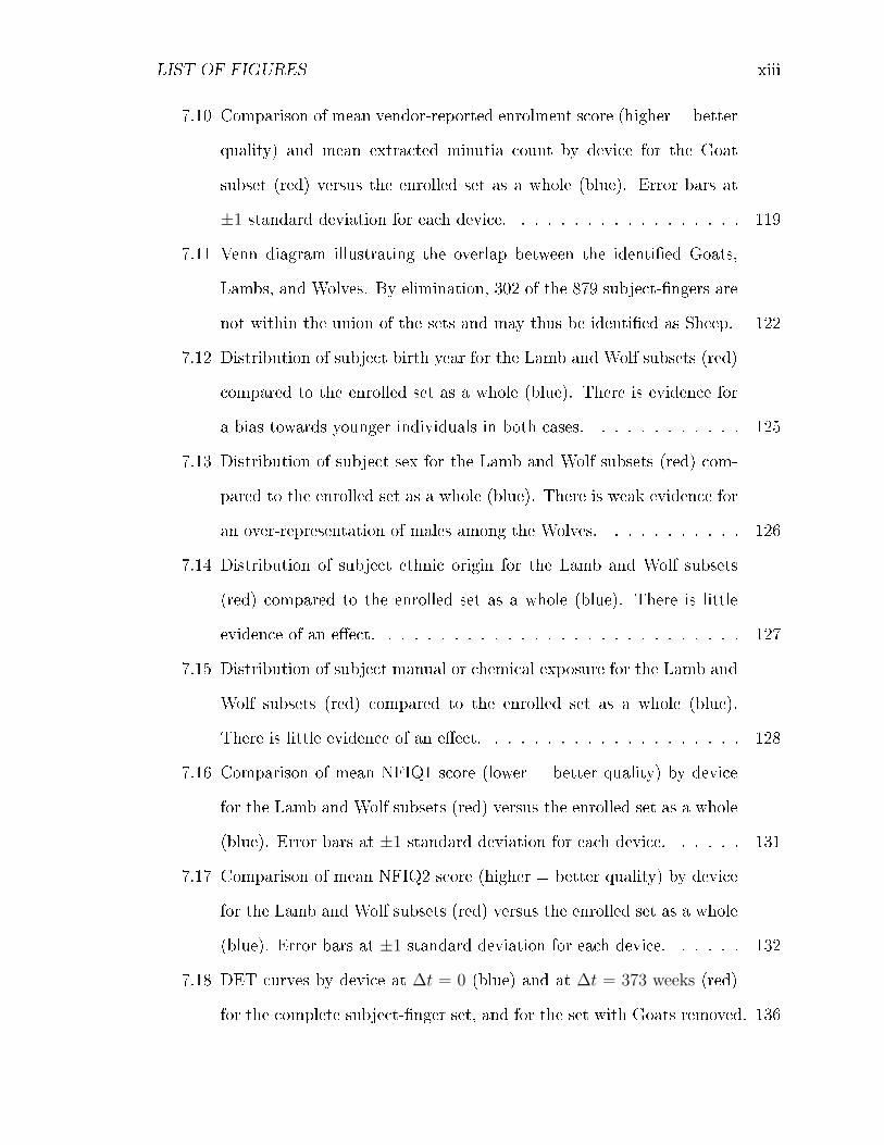
7.10 Comparison of mean vendor-reported enrolment score (higher = better
quality) and mean extracted minutia count by device for the Goat
subset (red) versus the enrolled set as a whole (blue). Error bars at
±1 standard deviation for each device. . . . . . . . . . . . . . . . . . 119
7.11 Venn diagram illustrating the overlap between the identi�ed Goats,
Lambs, and Wolves. By elimination, 302 of the 879 subject-�ngers are
not within the union of the sets and may thus be identi�ed as Sheep. 122
7.12 Distribution of subject birth year for the Lamb and Wolf subsets (red)
compared to the enrolled set as a whole (blue). There is evidence for
a bias towards younger individuals in both cases. . . . . . . . . . . . 125
7.13 Distribution of subject sex for the Lamb and Wolf subsets (red) com-
pared to the enrolled set as a whole (blue). There is weak evidence for
an over-representation of males among the Wolves. . . . . . . . . . . 126
7.14 Distribution of subject ethnic origin for the Lamb and Wolf subsets
(red) compared to the enrolled set as a whole (blue). There is little
evidence of an e�ect. . . . . . . . . . . . . . . . . . . . . . . . . . . . 127
7.15 Distribution of subject manual or chemical exposure for the Lamb and
Wolf subsets (red) compared to the enrolled set as a whole (blue).
There is little evidence of an e�ect. . . . . . . . . . . . . . . . . . . . 128
7.16 Comparison of mean NFIQ1 score (lower = better quality) by device
for the Lamb and Wolf subsets (red) versus the enrolled set as a whole
(blue). Error bars at ±1 standard deviation for each device. . . . . . 131
7.17 Comparison of mean NFIQ2 score (higher = better quality) by device
for the Lamb and Wolf subsets (red) versus the enrolled set as a whole
(blue). Error bars at ±1 standard deviation for each device. . . . . . 132
7.18 DET curves by device at ∆t = 0 (blue) and at ∆t = 373 weeks (red)
for the complete subject-�nger set, and for the set with Goats removed. 136
LIST OF FIGURES xiv
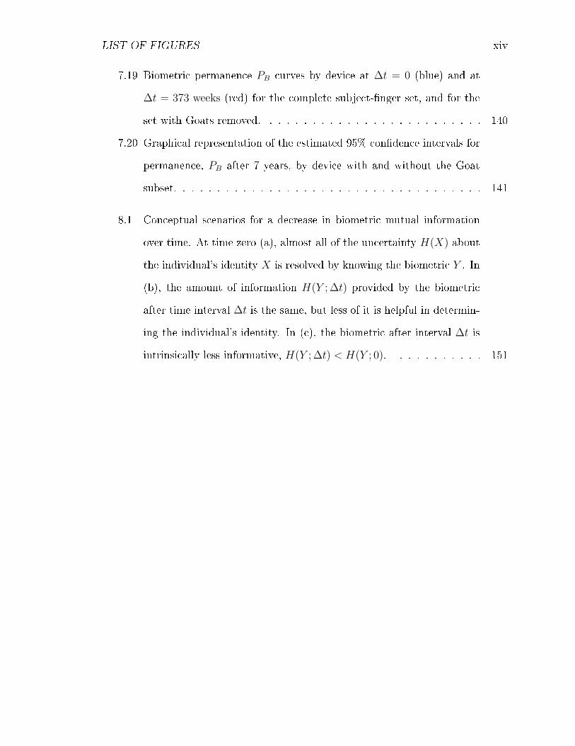
7.19 Biometric permanence PB curves by device at ∆t = 0 (blue) and at
∆t = 373 weeks (red) for the complete subject-�nger set, and for the
set with Goats removed. . . . . . . . . . . . . . . . . . . . . . . . . . 140
7.20 Graphical representation of the estimated 95% con�dence intervals for
permanence, PB after 7 years, by device with and without the Goat
subset. . . . . . . . . . . . . . . . . . . . . . . . . . . . . . . . . . . . 141
8.1 Conceptual scenarios for a decrease in biometric mutual information
over time. At time zero (a), almost all of the uncertainty H(X) about
the individual's identity X is resolved by knowing the biometric Y . In
(b), the amount of information H(Y ; ∆t) provided by the biometric
after time interval ∆t is the same, but less of it is helpful in determin-
ing the individual's identity. In (c), the biometric after interval ∆t is
intrinsically less informative, H(Y ; ∆t) < H(Y ; 0). . . . . . . . . . . 151
List of Tables
3.1 Pseudonymized devices and sensor technologies. . . . . . . . . . . . . 22
3.2 Dates of data collection visits . . . . . . . . . . . . . . . . . . . . . . 23
3.3 Numbers of genuine and imposter scores. . . . . . . . . . . . . . . . . 25
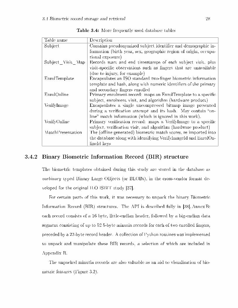
3.4 More frequently used database tables . . . . . . . . . . . . . . . . . . 28
5.1 Estimated 95% con�dence intervals for permanence, PB after 7 years,
by device. . . . . . . . . . . . . . . . . . . . . . . . . . . . . . . . . . 51
5.2 Relative e�ect of the imposter distributions to the RMS change in
match score discriminability, by device. . . . . . . . . . . . . . . . . . 65
6.1 Excluded percentages x of the lowest quality NFIQ-1 class (Class 5)
and the corresponding thresholds (lower xth percentiles) for exclusion
from NFIQ-2 . . . . . . . . . . . . . . . . . . . . . . . . . . . . . . . 91
6.2 Included percentages x of the highest quality NFIQ-1 class (Class 1)
and the corresponding thresholds (upper xth percentiles) for inclusion
from NFIQ-2 . . . . . . . . . . . . . . . . . . . . . . . . . . . . . . . 93
7.1 Subject-�ngers with the highest number of false non-matches over all
devices and visits, and which together constitute 50% of the false non-
matches when the overall FNMR is constrained to 5 %: we refer to
these as the Goat set. . . . . . . . . . . . . . . . . . . . . . . . . . . . 104
7.2 Finger positional identi�cation (�FingerPosition�) numbers . . . . . . 105
xv

LIST OF TABLES xvi
7.3 Fisher exact test for the signi�cance of subject sex. . . . . . . . . . . 112
7.4 χ-squared goodness-of-�t test for the signi�cance of subject birth year
at time of enrolment. . . . . . . . . . . . . . . . . . . . . . . . . . . . 113
7.5 χ-squared goodness-of-�t test for the signi�cance of subject self-reported
ethnic origin. . . . . . . . . . . . . . . . . . . . . . . . . . . . . . . . 113
7.6 χ-squared goodness-of-�t test for the signi�cance of subject manual or
chemical exposure. . . . . . . . . . . . . . . . . . . . . . . . . . . . . 113
7.7 One-tailed tests of signi�cance for the di�erence of mean NFIQ-1 be-
tween Goats and subject-�ngers as a whole. . . . . . . . . . . . . . . 116
7.8 One-tailed tests of signi�cance for the di�erence of mean NFIQ-2 be-
tween Goats and subject-�ngers as a whole. . . . . . . . . . . . . . . 120
7.9 One-tailed tests of signi�cance for the di�erence of mean vendor-reported
enrolment image quality and minutia count between Goats and subject-
�ngers as a whole. . . . . . . . . . . . . . . . . . . . . . . . . . . . . . 120
7.10 only �rst 30 rows shown Subject-�ngers pairs with the highest number
of false matches over all devices and visits, and which together consti-
tute 50% of the false non-matches when the overall FMR is constrained
to 5 %: we refer to these as the Lamb-Wolf set. . . . . . . . . . . . . 123
7.11 Fisher exact test for the signi�cance of subject sex. . . . . . . . . . . 124
7.12 χ-squared goodness-of-�t test for the signi�cance of subject birth year
at time of enrolment. . . . . . . . . . . . . . . . . . . . . . . . . . . . 124
7.13 χ-squared goodness-of-�t test for the signi�cance of subject self-reported
ethnic origin. . . . . . . . . . . . . . . . . . . . . . . . . . . . . . . . 129
7.14 χ-squared goodness-of-�t test for the signi�cance of subject manual or
chemical exposure. . . . . . . . . . . . . . . . . . . . . . . . . . . . . 129
7.15 One-tailed tests of signi�cance for the di�erence of mean NFIQ-1 be-
tween Lambs/Wolves and subject-�ngers as a whole. . . . . . . . . . 130

LIST OF TABLES xvii
7.16 One-tailed tests of signi�cance for the di�erence of mean NFIQ-2 be-
tween Lambs/Wolves and subject-�ngers as a whole. . . . . . . . . . 130
7.17 Estimated 95% con�dence intervals for permanence, PB after 7 years,
by device, with and without the Goat subset. Ns is the count of distinct
subject-�ngers in the sets, and is intended to give an indication of the
fraction of �ngers that would be excluded. . . . . . . . . . . . . . . . 137

Chapter 1
Introduction
Biometrics refers to the use of certain characteristic attributes of an individual's
person or behaviour in order to identify them or con�rm their claimed identity �
from the individual's face, �ngerprint, or pattern of vasculature to their voice, gait or
even heartbeat. They are deployed in applications ranging from unlocking a personal
communication device such as a cellphone or tablet, authenticating to social media
and banking apps, right up to government-issued identity documents such as biometric
passports, visas and electronic travel authorizations.
1.1 Problem statement
The desireable properties of a biometric characteristic, enumerated by Jain in Hand-
book of Biometrics [42] are:
1 Universality
2 Uniqueness
3 Permanence
4 Measurability
1

1.1 Problem statement 2
5 Performance
6 Acceptability
7 [resistance to] Circumvention
Some of these properties are easy to comprehend. By Universality for example,
we mean that the chosen trait should (for both operational and ethical reasons)
exclude from participation as few individuals as possible: a gait-based biometric
would exclude wheelchair users, while iris biometrics may disadvantage individuals
with certain types of eye disease, such as cataracts [76]. Measurability addresses
concerns of acquisition convenience, and leads us to favour �ngerprints over toe-
prints for example, since access to the former is less likely to require removal of
clothing. Resistance to circumvention encompasses anti-spoo�ng measures such as
sensor fusion [62] and liveness detection [24].
Meanwhile Performance has a natural de�nition in terms of the binary classi-
�cation problem [19], by which an individual's biometric presentation is classi�ed
as either a �match� or a �non-match� according to some decision rule, with well-
established metrics � the Type I and Type II error rates, conventionally termed False
Match Rate (FMR) and False Non-Match Rate (FNMR) in the biometric context �
and comparison tools such as the Decision Error Tradeo� (DET) curve [83].
The properties of Uniqueness and Permanence are less well established. In the
context of a biometric Identity Management System (IDMS), they concern the ability
to distinguish unambiguously between any two individuals in a given cohort, and to
continue to do so for as long as required by the particular application - such as the
duration of a biometric electronic travel authorization (ETA). While several biometric
modalities have established track-records of utility in such applications, this does
not necessarily establish that they provide a permanent and unique record of an
individual.
1.1 Problem statement 3
The concept of the uniqueness of a single object (such as a biometric record)
is a di�cult one, both philosophically and mathematically. In the mid twentieth
century, Kolmogorov and others developed the notion of algorithmic complexity (see
for example Li & Vitányi §2.8 [50]) to quantify the information in an object in terms
of its shortest possible description in some universal programming language. To the
author's knowledge, no attempt has been made to apply such methods in the �eld
of biometrics: instead, biometric uniqueness is approached practically in terms of
classi�cation performance. That is, a biometric record is considered unique if it can
reliably be distinguished from any other record.
In the particular case of �ngerprints, Tabassi et al. in the US National Institute for
Standards and Technology (NIST) have used machine learning techniques to identify
sets of features that are likely to result in good classi�cation accuracy (high genuine
match score, low imposter match score) resulting in the public release of the NIST
Fingerprint Quality (NFIQ) algorithms [74, 73].
From an information-theoretic point of view, a �nite length string or data record
can only convey a �nite amount of information about an individual: in particular,
there is an obvious lower bound of log2M bits required in order to uniquely index the
members of a cohort of sizeM . The Data Processing Inequality (see for example Cover
& Thomas §2.8 [9]) asserts that no subsequent processing can increase information
content: so the sequence of steps from a physical attribute (such as a �nger), to an
image of that attribute, to a set of features (such as a �ngerprint minutia record)
describing that attribute each tends to reduce its information content � and hence its
uniqueness. In the information-theoretic view, permanence becomes a question of the
extent to which the mutual information between a biometric record and the physical
attribute upon which it is based remains constant: that is, biometric template ageing
expresses a decrease in mutual information over time. Some questions that arise
naturally are:
1.1 Problem statement 4
� How should we de�ne biometric permanence (or template ageing) in a way that
is operationally meaningful?
� How can we estimate the magnitude of such ageing, in the presence of confound-
ing factors such as environment and operator acclimation?
� Where di�erent biometric capture technologies and feature extraction algo-
rithms exist within a modality, is template ageing observed consistently between
them?
� Do currently available measures of biometric quality adequately predict classi-
�cation performance?
� To what extent can such biometric quality metrics be used to improve the overall
classi�cation performance of a biometric IDMS?
� What demographic factors a�ect biometric quality (and, by extension, biometric
IDMS performance)?
� Are the same demographic factors signi�cant in the observed template ageing?
It should be noted that while we may refer throughout this work to properties
such as quality and permanence as characteristics of a biometric, they are (to the
extent that we can evaluate them) in fact properties of a whole biometric system,
in which everything from the underlying physiological trait, through the capture,
processing and storage of a biometric record, to the match scoring and classi�cation
algorithm play their roles. In particular, when we consider (in Chapters 6 and 7) the
demographics of �ngerprint quality and classi�cation performance, it is important
to note that the design of the capture systems, the selection of features, and the
training of scoring and classi�cation algorithms may be as important as any intrinsic
demographic factors of the underlying trait.
1.2 Goals 5
In the case of template ageing, one might suspect that physical degradation of
the sensor (such as scratching or marring of the platen) could be a signi�cant non-
physiological factor. In principle, one might try to minimize this by procuring a
number of identical devices from each manufacturer and using a new one for each
data collection phase. Unfortunately such a procedure was beyond the scope of this
study.
1.2 Goals
The goal of this work is �rstly to develop an operationally meaningful estimate of
biometric template ageing, and to apply it in a multi-year longitudinal �ngerprint
matching study. Secondly, to investigate the relationships between available measures
of biometric quality, subject demographics, and classi�cation performance in the same
data. Finally to apply these �ndings on quality and demographics to the problem of
template ageing.
1.3 Contributions
1.3.1 Methodology for estimating biometric permanence
In Chapter 4 we develop and de�ne a measure of template ageing which we call bio-
metric permanence PB, based on the change in FNMR (at a given FMR) between the
template ageing interval under test, and a short-time test. While intuitive, this de�-
nition of PB is practically di�cult to apply to estimate small changes in permanence
in a longitudinal study subject to experimental error and visit-to-visit systematic bi-
ases. To address this issue, we introduce the �matched delta� method. Comparisons
of these methods are performed using simulated data, and it is determined that the
new method showed dramatically reduces sensitivity to systematic biases.
1.3 Contributions 6
1.3.2 Observation and quanti�cation of template ageing
In Chapter 5 we apply the preceding methodology to data collected in a multi-year,
multi-vendor experimental �ngerprint acquisition and matching study, involving over
350 participants, with a gallery size in excess of 12,000 ISO/IEC standards-compliant
two-�nger biometric enrolment templates obtained with a variety of commercially-
available �ngerprint sensor technologies. Con�dence intervals for template ageing
are estimated using non-parametric methods. The behaviours of di�erent vendors'
devices are compared and contrasted, and limitations of the methodology identi�ed
and discussed.
1.3.3 Investigation of the e�ect of biometric data quality on classi�-
cation performance
In Chapter 6 we apply the NIST NFIQ �ngerprint quality measures to the images
collected in our study, comparing and contrasting the results for NFIQ-1 and NFIQ-2
across di�erent device technologies. We investigate the relationship between reported
quality and match score, for both genuine and imposter matches, and between quality
score and classi�cation performance. In particular, we con�rm that the overall clas-
si�cation performance may be improved by rejecting a fraction of �ngerprints based
on their quality.
Interestingly, for our data, we �nd that NFIQ-1 and NFIQ-2 are equally e�ective at
identifying any given fraction of low-quality presentations: the operational advantage
of NFIQ-2 is that its more expressive quality scale allows the rejection fraction to be
chosen much more precisely.
1.4 Publications 7
1.3.4 Observation and demographics of a biometric menagerie
In Chapter 7 we adapt a taxonomy �rst introduced by Doddington [17] in order to
identify subsets of `Goats', `Lambs', and `Wolves' in our data. We establish that these
categorizations are to a large degree common across di�erent �ngerprint capture de-
vices, and hence substantially re�ect intrinsic properties of the underlying biometric.
The demographics of the taxonomic subsets are explored: we �nd that, for our data,
females and older individuals are overrepresented in the Goat subset (those individ-
uals whose �ngerprints contribute disproportionately to the FNMR), while younger
individuals are overrepresented among the Lamb and Wolf subsets (the individuals
whose �ngerprints contribute disproportionately to the FMR). We discuss the extent
to which these di�erences might be explained by training bias in the classi�cation
algorithms. Finally, we examine the impact of the Goat subset on template age-
ing, observing a signi�cant improvement in biometric permanence when the subset is
removed.
1.3.5 Outline for a biometric channel model
While the development of a comprehensive information-theoretic treatment of bio-
metrics has remained an aspirational goal, it proved out of reach of the present work.
However some steps towards a biometric channel model are outlined in the concluding
chapter.
1.4 Publications
The following publications are based on the work presented in this thesis:
� In Proceedings of the 2017 Annual IEEE International Systems Conference
(SysCon): J. Harvey, J. Campbell, S. Elliott, M. Brockly and A. Adler Bio-
metric Permanence: De�nition and Robust Calculation [31]

1.4 Publications 8
� In IEEE Transactions on Instrumentation and Measurement : J. Harvey, J.
Campbell and A. Adler Characterization of Biometric Template Aging in a
Multiyear, Multivendor Longitudinal Fingerprint Matching Study [30]
Chapter 2
Background and literature review
2.1 History and early application of biometrics
While in its broadest sense, the term biometrics has historically been used to denote
the measurement and statistical analysis of biological data in general [10] � which
nowadays might more likely be referred to as biostatistics � it is now almost universally
understood to mean the use of biological traits to establish or con�rm the identity
of an individual [42]. Among the biometric traits (or modalities) that have been
studied and/or employed for this purpose include the features and morphology of
the face [54], an iris image [46], a pattern of blood vessels [7], or an analysis of the
individual's voice [69] or gait [51]. The focus of this work is the biometric modality
of �ngerprints [53].
Interest in the features of the human hand has a long cultural history from the
point of view of their purported usefulness for divination or �cheiromancy� [6], but
its modern development as a biometric modality really begins during the nineteenth
century: Galton [25] gives a more-or-less contemporary (albeit subjective) account.
Although his own primary interest seems to have been what the study of �nger-
prints might reveal about heredity, biological symmetry (homochirality) and specia-
9
2.2 Modern biometrics 10
tion, Galton devotes a whole chapter to their application to personal identi�cation;
in particular, the use of �signs-manual� in place of conventional written signatures in
the attestation of contract documents, the pioneering of which he attributes to Sir
William Herschel (and which was subsequently reported by him [33]). Galton also
discusses the then-emerging forensic use of �ngerprinting, �rst noting its distinction
as a �much more di�cult� one-to-many (identi�cation) task rather than a one-to-one
(veri�cation) task, and going on to consider how even a relatively simple �A.L.W.�
(arch-loop-whorl) �ngerprint classi�cation scheme might greatly improve the utility
of the French anthropomorhic system [3] of Bertillonage. Such a scheme was then
already in use by police in Calcutta (now Kolkata), India under the direction of
Henry [32] and latterly substantially attributed to Haque [70]. Roughly contempora-
neous contributions in other jurisdictions, especially those of Vucetich in Argentina
and Brazil, are also noted in a historical survey by Polson [59].
It should be noted that the Henry-Haque classi�cation scheme was based on a
coarse attribution of each �nger's dominant feature, rather than the kind of minutia-
based classi�cation of single �ngers provided by the devices used in the present work
- although Galton (op. cit.) at least was familiar with the concept and terminology of
�ngerprint minutiae: one of the appealing features was its ability, after application of
a coding scheme due to Bose [4], to be transmitted telegraphically � a valuable factor
given the rise of mass transportation and the increased mobility of criminal suspects.
2.2 Modern biometrics
While much of the early history and development of biometric techniques focused on
the identi�cation and apprehension of criminal suspects, progress in automated cap-
ture, feature extraction, and algorithmic matching technologies has allowed biometrics
to expand into the �elds of large-scale identity management systems (IDMS). Such
2.2 Modern biometrics 11
schemes include those for machine readable travel documents [29], trusted traveller
programs [78], and governmental personal identity veri�cation (PIV) programs [28].
2.2.1 Renewable biometric references
Password and public key infrastructure (PKI) based authentication systems provide
the ability for an issuer to revoke and renew credentials simply by deleting passwords
or keys and inserting new, randomly generated, ones. In contrast, raw biometric
records provide limited opportunity for revocation or renewal - as noted by Shreier
et al., �we have one face, two irises, 10 �ngers� [66]. Considerable interest has been
directed to addressing this de�ciency in order to develop what have become known as
renewable biometric references (RBRs) [39]. A key goal of such e�orts is to protect
the personally identi�able information (PII) of the individual [44, 43] while providing
su�cient immunity to a variety of potential compromizes including attacks via record
multiplicity (ARM), surreptitious key-inversion (SKI), and blended substitution at-
tacks (BSI) [65].
2.2.2 Forensic applications
The matching of latent �ngerprint (or partial �ngerprint) images recovered from
scenes-of-crime remains an important application of biometrics [52], with much cur-
rent attention given to pre-processing of latent �ngerprints [49], especially using chem-
ical [21] and spectroscopic [11] techniques. Unlike many other biometric applications,
that are dominated by one-to-one (or biometric veri�cation) matches, forensic biomet-
rics may include one-to-many (or biometric identi�cation) tasks, such as identifying
a list of suspects from an existing criminal database, as well as the association of
criminal cases based on collection of latent �ngerprints from an unknown common
subject [52]. Biometric quality and template ageing are surely relevant to these ap-
plications, however they may have additional domain-speci�c aspects that are not
2.3 Biometric template ageing 12
addressed in the present work - such as assessing the biometric quality of partial
prints.
2.3 Biometric template ageing
An assumption underlying the deployment of biometric IDMS systems is the stability
of the chosen biometric features � that is, that the biometric trait will remain, over
the expected lifetime of the credential, su�ciently similar to that of the template to
enable a positive comparison. In applications such as biometrically-enabled passports,
stability over a period of �ve or ten years is desirable in order to align with current
renewal policies for such credentials [36]. From a physiological point of view however,
it is natural to expect some change in traits over time. For example, a subject's loss
or gain in weight may a�ect measurements of hand geometry [68], while the onset
of degenerative disease, injury, or occupational damage may a�ect �ngerprints [18,
12]. As an instrumentation and measurement problem, biometric capture has in this
respect something in common with many clinical monitoring and medical imaging
systems: that is, the systems should be sensitive to clinically signi�cant changes (in
the case of biometrics, a change of identity) while remaining relatively insensitive to
benign morphological changes arising from simple ageing or weight gain for example.
Slow changes in biometric features over time are typically referred to as template
ageing [82, 79], and the performance of large-scale systems can be in�uenced by this
e�ect. Unfortunately template ageing is hard to measure, because it is very sensitive
to the visit-to-visit variability inherent in such a study (e.g. test personnel [5], test
equipment and weather [20, 71]).
Attempts to quantify biometric permanence in fact go right back to Galton (op.
cit.), who devoted an entire chapter to observations on the persistence of �ngerprint
minutiae in an (admittedly small) sample of 15 individuals. In one case, the inter-
2.3 Biometric template ageing 13
val between observations was as large as 31 years, while in another he was able to
record prints of a juvenile individual (aged approximately two-and-a-half years) and
subsequently compare them to those obtained at age 15 years. Galton estimated that
he could identify, on average, 35 �points of interest� (minutiae) from each digit, and
that of the 700 such points provided by a full set of 10 �ngerprints, 699 could be �in-
ferred� to remain throughout an individual's life (and beyond - based on �ngerprints
apparently having been obtained from Egyptian mummies).
Modern attempts to quantify permanence (or template ageing) are generally based
on statistical analyses of large numbers of biometric enrolments. The age progression
of biometric traits has perhaps received most attention within the facial recognition
and iris recognition modalities. Manjani et al. [54] evaluated both 2D and 3D facial
recognition algorithms on a dataset of sixteen participants acquired over a period
of ten years, comparing genuine acceptance rate (GAR) at 0.1% false acceptance
rate (FAR) for short-term intervals (less than three months between enrolment and
veri�cation) versus long-term intervals (more than �ve years between enrolment and
veri�cation). Unlike the present work, the intervals were not blocked into absolute ac-
quisition times i.e. all intervals greater than �ve years were taken together. They were
able to reject at α = 0.05 the null hypothesis that the short- and long-term genuine
scores were drawn independently from normal distributions of equal mean and vari-
ance (t-test), or from the same continuous distribution (Kolmogorov-Smirnov test).
In the case of the algorithm that performed best over the long-term intervals (�3D
Region Ensemble: Product�), they found weak evidence against the corresponding
hypotheses for the imposter scores: this is consistent with our model, in which the
imposter distribution was assumed to be constant.
Lanitis & Tsapatsoulis [48] proposed a measure of biometric ageing that they called
�Aging Impact� (AI), derived from the homogeneity and dispersion of a collection of
templates. Although the primary focus of their work concerned facial images, �nger-
2.3 Biometric template ageing 14
and palm-print images were also considered; however they applied their method to
individuals within di�erent age classes, rather than to repeated measures of the same
individuals over time as in the present work. The focus of much subsequent work
has been the development and evaluation of arti�cial age progression algorithms for
forensic applications [47, 58], rather than for biometric IDMSs.
Template ageing has also been reported in the iris modality [22, 26]. Hofbauer
et al. [34] noted some controversy about its existence, and discussed the di�culty
of controlling confounding factors independently � in particular, the cases of illumi-
nation and pupillary dilation. There was only a single long-term time interval � in
this case of four years � while the study consisted of data from 47 subjects. The
authors considered two schemes for re-normalization of pupil diameters: a �rubber
sheet model� (RSM) and a �biomedical model� (BMM). They showed that while such
re-normalizations were somewhat e�ective in improving long-term match accuracy,
there was still a decrease in performance between intra-year and inter-year compar-
isons. This suggests that while systematic changes in pupillary diameter are a factor
in iris template ageing, they are not the only such factor. Signi�cant degradation
over time in genuine iris match scores have been reported elsewhere [13].
Fingerprint ageing might be expected to share some of the same physiological
factors as face ageing � in particular, skin textural changes and loss of tissue elasticity
� and has been reported by Uludag et al. [77], who addressed the case of typicality
and/or variability between presentations of the same biometric using novel template
selection algorithms, based either on clustering or on mean distance. They then
used this template selection to evaluate a number of template update schemes. They
found that a scheme in which an original template was updated selectively using
later presentations (�AUGMENT-UPDATE�) outperformed one in which the original
template data were discarded altogether (�BATCH-UPDATE�). From this, we might
infer that the magnitude of the template ageing e�ect was not signi�cantly greater
2.4 De�nition and evaluation of biometric data quality 15
than that of the intraclass variance, at least over the relatively short interval of their
study (approximately four months). Template ageing has recently been reported in
two non minutia based �ngerprint matching schemes [45]: FingerCode (FC), a Gabor-
�lter based technique similar to the widely adopted IrisCodes of Daugman [14]; and
Phase Only Correlation (POC).
Template ageing has also been observed in speech biometrics [82].
Meanwhile, the in�uence of biometric sample quality on template ageing was
highlighted by Ryu et al. [64], who found that lower sample quality (evaluated using
the NIST NFIQ measure [74]) was associated with an increased number of matching
errors.
The social and ethical implications of biometric ageing have also received recent
attention [61]: most notably the potential role of biometrics in the �problematisation
of ageing and of older people�. The authors are careful to distinguish between a bio-
metric subject's chronological age and biometric template ageing: their arguments
for the exclusionary potential of the former (which is known to a�ect biometric sys-
tem performance [67]) are stronger than those for the latter, which rely on a rather
subtle semiotic analysis of the relationship between biometric features, subject, and
biometric system as a whole.
2.4 De�nition and evaluation of biometric data quality
Jain [42] identi�es a number of properties that are desirable in a biometric char-
acteristic, including uniqueness and permanence; performance and (resistance to)
circumvention. Performance here may be interpreted as the system's ability to cor-
rectly identify the biometric presentation of a genuine subject, and to correctly reject
the biometric presentation of an imposter subject. As with any such pattern classi-
�cation problem, these abilities are inherently con�icting, and represent the Type I
2.4 De�nition and evaluation of biometric data quality 16
and Type II error probabilities of a classical Neyman-Pearson hypothesis test [57]
or signal detection problem. As such, biometric systems typically reduce the deter-
mination to a one-dimensional similarity score which may be thresholded in order
to obtain a match/non-match decision; by appropriate choice of the decision thresh-
old, the system integrator or operator may trade o� security (lower false accept rate,
FAR) against convenience (lower false reject rate, FRR) to suit the requirements of
the particular IDMS application.
At any particular threshold, the fundamental performance (i.e. the minimum ob-
tainable FRR at a chosen FAR, or vice-versa) will be intrinsically limited by the
separability of the subjects' biometric characteristics over some biometric feature
space. In the case of �ngerprints (the focus of this proposed work), the feature space
is usually a space of extracted �ngerprint minutiae types and locations. In general,
we would expect a feature space of higher dimensionality (more independent fea-
tures) to permit higher classi�cation accuracy. Features are, however, not always
informative: in particular, the set of features that best describes a population may
not coincide with that which best discriminates between its classes. Thus in the case
of facial recognition for example, linear classi�ers based on discriminant analysis (so-
called �Fisherfaces�) may outperform those based on principal component analysis
(PCA) [2] (or �eigenfaces�).
If biometric performance is de�ned in terms of classi�cation accuracy in this way,
then uniqueness is essentially a measure of intrinsic performance (i.e. the classi�cation
accuracy that might be obtained in the absence of any variability in the collection
and/or processing of the biometric). Permanence becomes a measure of how well
discriminability is maintained over time. These three characteristics each represent
aspects of the informativeness of the biometric; in fact Adler et al. have sought to
de�ne biometric information formally in this sense as
�the decrease in uncertainty about the identity of a person due to a set of
2.4 De�nition and evaluation of biometric data quality 17
biometric measurements� [1]
In this view, one might expect a biometric's resistance to circumvention also to
be related to its performance, since an attacker would need to expend more e�ort
to spoof a more informative record - although in practice, external measures such
as liveness detection and/or multi-factor authentication requirements are likely to be
more signi�cant.
Grother & Tabassi were among the �rst to formalize the evaluation of biometric
quality as a predictor of genuine match score [27]. In particular, they addressed the
fact that de�ning quality in this way necessarily involves the interaction of at least
two biometric presentations1 whereas, to posses utility, the quality measure so de-
rived should be applicable to a single presentation. They discuss the appropriateness
of various quality combination functions in order to explore the dependence of simi-
larity score on match pairs of di�ering quality, as well as the useful number of levels
of quantization of biometric quality. Distinctions were highlighted between positive
identi�cation (veri�cation) applications, in which an enrolled subject is �motivated
to submit high quality samples�, and negative identi�cation (blacklist) applications,
where an individual is perhaps enrolled unwillingly and may be motivated to obscure
or obfuscate their biometric: in the former case, they identi�ed the key performance
metric as false non-match rate (FNMR), while in the latter it is false match rate
(FMR). They demonstrated the dependence of similarity score on quality in the pos-
itive identi�cation case through the use of error versus reject curves. The notion of
an ideal quality metric for the positive identi�cation case was developed as follows:
Suppose a system is operating at a FMR determined by operational security re-
quirements. There will be an associated FNMR x-%, meaning that x-% of genuine
biometric classi�cation scores fall below the decision threshold for that FMR, and are
misclassi�ed as imposters. An ideal quality metric for this case would be one that
1It may be more than two, since template generation may be based on multiple enrolment pre-sentations.
2.5 The biometric menagerie 18
identi�es exactly these presentations, and removes them from consideration - thereby
reducing the FNMR to zero.
This formalism was applied in the development of the NIST NFIQ [74] and NFIQ-
2 [73] �ngerprint quality algorithms used in the present work.
2.5 The biometric menagerie
Doddington introduced the idea of a �biometric zoo� [17] to describe the subject-
dependence of biometric classi�cation errors, originally applying it in the speaker
veri�cation modality. Four categories of individuals were posited: those whose bio-
metric matched poorly against itself, and which therefore contributed disproportion-
ately to the FNMR, were labelled �Goats�; those whose biometric was easily imper-
sonated2 as �Lambs�, and those whose biometric is easily mis-attributed to such lambs
as �Wolves�, with Lambs and Wolves together contributing disproportionately to the
FMR. Remaining individuals were classi�ed, by elimination, as �Sheep�. Similar cat-
egorizations have since been established in the face [81], iris [72] and �ngerprint [80]
modalities; the latter identifying Lambs and Wolves in a multi-�nger dataset obtained
from 510 individuals; Goats could not reliably be identi�ed because of the relatively
small number of genuine matches3.
The biometric menagerie has subsequently been re�ned by considering the in-
teractions of genuine and imposter scores [84]. The question of whether such cate-
gorizations generalize across biometric matching algorithms and data sets has been
investigated by Teli et al. [75]. More recently, the concept of a biometric menagerie
has been applied to biometric template update procedures [60] and to biometric fu-
sion [63]. We believe that the present work is the �rst to extend the concept speci�-
2The term impersonation does not necessarily imply an actively malicious actor here: we areoften interested in so-called zero e�ort imposters � individuals whose biometric naturally closelyresembles that of another.
3Although the number of individuals was larger than that of the present study, only a singleenrolment-veri�cation pair was collected for each.
2.6 Relationship between template ageing, quality, and demographics 19
cally to the subject-dependence of biometric permanence.
2.6 Relationship between template ageing, quality, and
demographics
A recent large-scale longitudinal study by Yoon & Jain examined both genuine and
imposter match scores versus template age, NIST NFIQ �ngerprint quality, and sub-
ject demographics [86]; the latter consisting of subject age, sex, and a binary race
variate. The study size was large, consisting of 10-�nger records of more than 15,000
subjects, with intervals between acquisitions ranging from �ve to twelve years. Boot-
strapped estimates of mean genuine match score showed clear decreasing trends with
time interval (i.e. template age), subject chronological age, and NFIQ score with only
marginal dependence on the other factors.4 Of the three signi�cant predictors, NFIQ
score was found to be the strongest. Although the e�ect size was large enough, for
these factors, to be estimated with high con�dence, the genuine and imposter score
distributions remained su�ciently separable over the duration of the study that there
was no observed change in either the true acceptance rate (i.e. 1− FRR) or false
acceptance rate (FAR).
Finally, Kirchgasser & Uhl attempted to relate observed biometric template age-
ing, over a four year interval, in the �ngerprint modality to decreases in biometric
quality [45], again using the NIST NFIQ metric of Tabassi (op. cit.) as well as
BRISQUE - a non �ngerprint speci�c measure of image spatial quality. However �
perhaps due to the relatively small study size of only 49 participants � they were
unable to do so, even observing some counter-intuitive negative correlation between
NFIQ score and genuine match score among false non-matches.
4A decreasing trend because NFIQ scores from 1 (best) to 5 (worst).
2.7 Open questions 20
2.7 Open questions
Yoon & Jain's study demonstrates an important feature of biometric template ageing:
namely, that changes in match score do not necessarily result in observable changes
in classi�cation performance - at least, not over the time periods available for study.
An open question therefore is how should we characterize template ageing in a way
that is operationally meaningful?
Comparing the results of Yoon & Jain with those of Kirchgasser & Uhl highlights
another important question: how can we estimate the magnitude of template ageing
robustly in smaller cohorts, where we do not have the advantages of large sample size
to reduce estimation variance?
Turning to issues of biometric quality, we would like to know how well the publicly-
available NFIQ metrics perform as predictors of classi�cation accuracy, in an indepen-
dent dataset collected under di�erent conditions and protocols than those on which
their classi�ers were trained. Demographic factors a�ecting biometric quality have
been reported by Yang [85], but the analysis did not consider the demographics of
classi�cation accuracy (or of template ageing) directly.
The study described in this thesis is somewhat larger than that of Kirchgasser &
Uhl and, although far smaller than that of Yoon & Jain, we believe that it supports
their main conclusions concerning template ageing in the �ngerprint modality, as well
as providing valuable additional evidence for the role of biometric quality and subject
demographics.
Chapter 3
The �Norwood� dataset
3.1 History and demographics
The data used for this study were collected in four phases between 2006 and 2013. The
�rst two phases, in 2006 and 2008, were collected as part of a study on biometric sys-
tem interoperability undertaken on behalf of the International Labour Organization
(ILO) and known as the �Seafarers' Identity Documents Biometric Interoperability
Test�, or ISBIT. Data collection in these phases, known as ISBIT-3 and ISBIT-4,
was undertaken by Bion Biometrics, Inc. with subject recruitment from a general
population in and around Ottawa,Canada.
In 2012, Carleton University, in collaboration with Bion Biometrics, obtained
funding from the National Research Council (NRC) in Canada for a project entitled
�E�ect of template ageing and sensor technologies in �ngerprint recognition� 1. The
project was to leverage and extend the database and software from the ISBIT studies,
with a re-focus towards template ageing. Funding was su�cient for a further two
phases of data collection, which were undertaken in 2012 and 2013. Vendors who had
provided �ngerprint capture devices and API software for the ISBIT studies were
approached to permit their use in the new study, and to renew software licences
1NSERC CRD428240-11
21
3.1 History and demographics 22
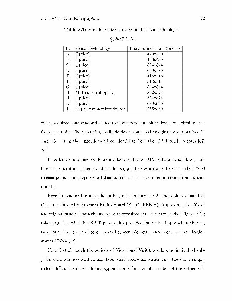
Table 3.1: Pseudonymized devices and sensor technologies.
©2018 IEEE
ID Sensor technology Image dimensions (pixels)A. Optical 420x480B. Optical 456x480C. Optical 524x524D. Optical 640x480E. Optical 416x416F. Optical 512x512G. Optical 524x524H. Multispectral optical 352x524J. Optical 524x524K. Optical 620x620L. Capacitive semiconductor 256x360
where required: one vendor declined to participate, and their device was eliminmated
from the study. The remaining available devices and technologies are summarized in
Table 3.1 using their pseudomomized identi�ers from the ISBIT study reports [37,
38].
In order to minimize confounding factors due to API software and library dif-
ferences, operating systems and vendor supplied software were frozen at their 2008
release points and steps were taken to isolate the experimental setup from further
updates.
Recruitment for the new phases began in January 2012, under the oversight of
Carleton University Research Ethics Board `B' (CUREB-B). Approximately 40% of
the original studies' participants were re-recruited into the new study (Figure 3.1);
taken together with the ISBIT phases this provided intervals of approximately one,
two, four, �ve, six, and seven years between biometric enrolment and veri�cation
events (Table 3.2).
Note that although the periods of Visit 7 and Visit 8 overlap, no individual sub-
ject's data was recorded in any later visit before an earlier one; the dates simply
re�ect di�culties in scheduling appointments for a small number of the subjects in
3.1 History and demographics 23
Table 3.2: Dates of data collection visits
Visit start (YYYY-MM-DD) Visit end (YYYY-MM-DD)1 2006-02-07 2006-03-032 2006-02-22 2006-03-243 2008-09-26 2008-10-154 2008-10-13 2008-10-275 2012-02-12 2012-03-036 2012-03-12 2012-03-317 2013-03-06 2013-04-228 2013-04-05 2013-04-27
the cohort.
Figure 3.1: Overlap of participants between data collection phases (the 2013 collec-tion is omitted for clarity; it overlaps almost completely with 2012).
©2018 IEEE

3.2 Data collection protocol 24
3.2 Data collection protocol
In our study, data were collected in four phases, each consisting of a pair of subject
visits separated by approximately two weeks in each of the years 2006, 2008, 2012 and
2013. Approximately 200 participants were recorded in each phase, with more than
100 taking part in at least two phases and over 70 being present in all four (Figure 3.1).
The protocol for each subject visit consisted of a sequence of two-�nger enrolments,
followed by a sequence of single-�nger veri�cation presentations [37, 38]. Preferred
�ngers for enrolment were right and left index in the �rst instance; however if either
of these was unavailable (or failed to enrol) alternate �ngers were o�ered in the order
right thumb, left thumb; right middle, left middle; right ring, left ring; and �nally
right and left �pinky� �ngers. In subsequent enrolments, previously enrolled �ngers
were preferred in order to maximize the number of potential genuine matches. Three
bitmapped images of each candidate �nger were captured during each enrolment,
and a further six images (in two distinct three-presentation veri�cation attempts) per
enrolled �nger during each veri�cation, such that a typical visit resulted in eighteen
single-�nger images per subject per device. In each subject visit, the order in which
devices were presented for both enrolment and veri�cation was randomized under
software control in order to counterbalance for subject and operator acclimation.
In order to minimize labelling errors, the captured images were examined at in-
tervals during or immediately after every visit by an experienced human operator2.
While this procedure cannot guarantee that �nger labelling is correct (i.e. that an
image labelled as �Subject k, �nger d� does in fact come from that subject-�nger) it at
least ensures, with high probability, that the labelling is consistent across all records
for a particular subject-visit. Images that were corrupted (due to malfunctions of
the device hardware or capture software for example) were also �agged during this
examination, and removed from the dataset at this stage.
2Dr. John Campbell, Bion Biometrics, Inc.

3.2 Data collection protocol 25
Table 3.3: Numbers of genuine and imposter scores.
©2018 IEEE
ID Genuine Imposter ID Genuine ImposterA 92243 24418495 G 62476 15301808B 93630 25282974 H 61698 14901522C 91326 24352257 J 57803 13646908D 98725 27124531 K 98872 27125117E 56047 14296890 L 99328 27350928F 98874 27215472 Tot. 911022 241016902
A custom data acquisition software program isbitDirector was provided as an in-
kind contribution to the project by Bion Biometrics, Inc. . In order to make the
subject visits more interesting (for both subjects and test operators), the veri�cation
protocol programmatically generates a pre-determined fraction - by default, 20% -
of imposter matches. These �online� matches are recorded in the database but are
not used for the data analysis: instead, a separate �o�ine� process isbitGrinder was
used to extract and crossmatch the desired sets of veri�cation images and enrolment
templates.
Twelve di�erent commercially-available �ngerprint sensor devices were initially
present in the study, representing multiple vendors and technologies: single-spectral
optical, multi-spectral optical and capacitive. One device became unreliable in the
later phases, and was dropped from the capture protocol. One further device became
unavailable due to software licensing restrictions and was removed from the study
altogether (Table 3.1). To our knowledge, all of the optical sensors are based on
frustrated total internal re�ection. Ages of the participants at the time of the most
recent collection ranged from 15 years to 70 years. In excess of 15,000 ISO/IEC
standards-compliant two-�nger biometric enrolment templates were generated, and
nearly 200,000 bitmapped single-�nger veri�cation images were collected: together,
these allowed us to synthesize nearly 250 million single-�nger match transactions,
with approximately 900,000 genuine (same subject, same �nger) matches (Table 3.3).
3.3 Study terminology and notation 26
3.2.1 Carleton modi�cations to the software and protocol
Because the ISBIT study was focused on vendor interoperability, the original isbit-
Grinder software was written to perform cross-matches between veri�cation images
obtained on one vendor's equipment and enrolment templates recorded by another
vendor's. For the purpose of this work, the software was modi�ed to eliminate these
inter-vendor cross-matches in favour of inter-visit matches.
3.3 Study terminology and notation
In this work, a visit comprises a sequence of biometric enrolments and veri�cation
attempts conducted on a set of subjects over a short contiguous period (typically 2-4
weeks). Match scores are generated between veri�cation images collected in the nth
visit, Vn and biometric templates obtained during the mth visit, Em (Table 3.2).
Although the - inherited - protocol used in this study is based on a two-�nger
biometric template, match scores are evaluated separately for each enrolled �nger.
Hence we de�ne a match score, sjinm between an image of subject-�nger j presented
during veri�cation visit Vn and the minutia record of subject-�nger i recorded during
enrolment visit Em. Although in principle both i and j are composed of a subject
identi�er (k say) and a �nger identi�er (d = 1, 2, . . . , 10), in practice the o�ine match
generating software isbitGrinder only makes same-�nger matches, i.e. barring mis-
labelling, genuine scores always correspond to same subject to same subject matches,
while imposter scores are between same �ngers of di�erent subjects.
It is important to note that whereas the veri�cation protocol takes the form of
a two-attempt transaction involving multiple individual presentations of a pair of
�ngers, all the performance metrics used in this work are based on single-�nger match
scores. So, for example, classi�cation performance is quanti�ed in terms of false match
rate, FMR, and false non-match rate, FNMR, rather than transactional measures such
3.4 Biometric record storage and retrieval 27
as false accept rate (FAR) or false reject rate (FRR).
3.4 Biometric record storage and retrieval
Along with data acquisition and match score generation software, Bion Biometrics,
Inc. provided data from the ISBIT phases of the study as a Microsoft SQL Server
(MSSQL) database. The database was re-used and updated to include the Norwood
phases at Carleton, with schema extensions as required to support the scienti�c ob-
jectives of this work � for example, additional tables for the biometric quality metrics
and attempted taxonomies of Chapter 6.
3.4.1 Database structure
The MSSQL database provides the primary interface to the biometric records, col-
lection timestamps and subject demographics whose analysis forms the basis of the
present work. Descriptions of some of the more frequently used database tables are
provided in Table 3.4. In addition to these, an `Algorithm' table is used when it is
required to map internal (proprietary) device designators to either the pseudonymized
identi�ers used for the experimental arrangement (�B (1)�, �H (2)� etc.) or those used
for the purpose of reporting (�Device L�, �Device A� and so on).
Although not used in the generation of match scores (which are based on compar-
isons between VerifyImage and EnrolTemplate records), the images captured during
enrolment, from which the template minutiae are extracted, are recorded in table
EnrolImage. These are used in the examination of biometric quality in Chapter 6.
Quality assessment was performed externally on both enrolment and veri�cation im-
ages, and additional tables were created as required to hold the re-imported quality
scores.
Sample MSSQL queries are provided in Appendix A.
3.4 Biometric record storage and retrieval 28
Table 3.4: More frequently used database tables
Table name DescriptionSubject Contains pseudonymized subject identi�er and demographic in-
formation (birth year, sex, geographic region of origin, occupa-tional exposure)
Subject_Visit_Map Records start and end timestamps of each subject visit, plusvisit-speci�c observations such as �ngers that are unavailable(due to injury, for example)
EnrolTemplate Encapsulates an ISO standard two-�nger biometric informationtemplate and hash, along with numeric identi�ers of the primaryand secondary �ngers enrolled
EnrolOnline Primary enrolment record: maps an EnrolTemplate to a speci�csubject, enrolment visit, and algorithm (hardware product)
VerifyImage Encapsulates a single uncompressed bitmap image presentedduring a veri�cation attempt and its hash. May contain �on-line� match information (which is ignored in this work).
VerifyOnline Primary veri�cation record: maps a VerifyImage to a speci�csubject, veri�cation visit, and algorithm (hardware product)
MatchPresentation The (o�ine generated) biometric match scores, re-imported intothe database along with identifying VerifyImageId and EnrolOn-lineId keys
3.4.2 Binary Biometric Information Record (BIR) structure
The biometric templates obtained during this study are stored in the database as
varbinary typed Binary Large OBjects (or BLOBs), in the cross-vendor format de-
veloped for the original ILO ISBIT study [37].
For certain parts of this work, it was necessary to unpack the binary Biometric
Information Record (BIR) structures. The API is described fully in [38], AnnexB:
each record consists of a 16 byte, little-endian header, followed by a big-endian data
segment consisting of up to 52 5-byte minutia records for each of two enrolled �ngers,
preceded by a 22-byte record header. A collection of Python routines was implemented
to unpack and manipulate these BIR records, a selection of which are included in
Appendix B.
The unpacked minutia records are also valuable as an aid to visualization of bio-
metric features (Figure 3.2).
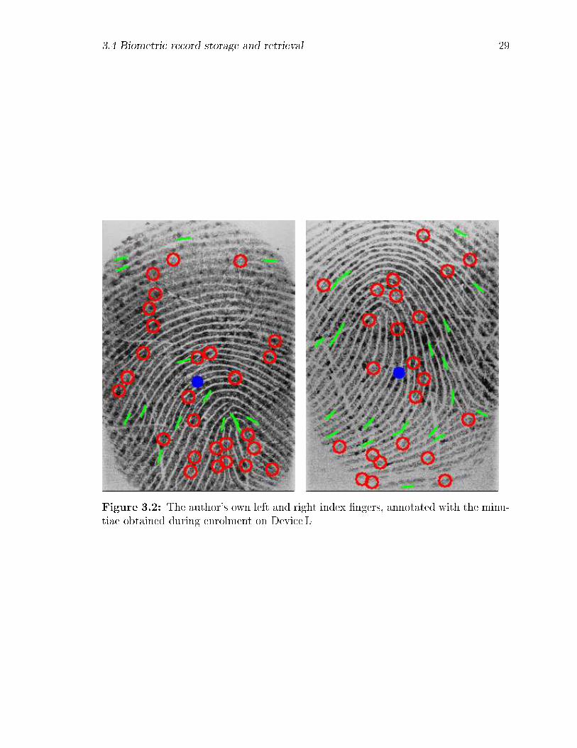
3.4 Biometric record storage and retrieval 29
Figure 3.2: The author's own left and right index �ngers, annotated with the minu-tiae obtained during enrolment on Device L
Chapter 4
Biometric permanence: de�nition and
robust calculation
4.1 Introduction
Biometric systems allow identi�cation of people based on analysis of images of their
biometric features [41]. When a biometric is used for veri�cation, a biometric sample
image is tested against a previously captured sample from the person to be veri�ed
[53]. In veri�cation, the performance of the system is measured in terms of its Type-I
and Type-II error rates. One key criterion for a biometric modality is the stability of
the underlying features. For example, for �ngerprint recognition, the structure of the
friction ridges is considered to be a unique and stable characteristic of each individual
[53].
However, it is widely known [82, 22, 55] that, for any biometric modality, some
degree of variation in the biometric features occurs over time. An example is the
damage that can occur to �ngerprints, which is more common in certain population
groups and occupations [18]. Variation in biometric features over time, known as tem-
plate ageing, results in a decrease in biometric recognition accuracy over time [40].
30
4.2 Methodology 31
The importance of template ageing varies across di�erent applications of biometrics.
It is especially signi�cant for many government programs, such as border security, in
which stored templates are intended to be used for comparison over years or decades.
There have been several studies done in assessing or describing the impact of template
ageing [64, 77]. However, many of these studies have very small datasets (in terms of
sample sizes and time periods). Several challenges associated with permanence were
identi�ed, including those associated with speci�c occupations and other environmen-
tal factors [20, 67]. Although biometric permanence has seen some investigation, to
our knowledge no statistical measures have been de�ned to measure it or calculate
it robustly. To address this de�ciency, we de�ne a new term, biometric permanence,
PB, and develop methods to calculate it. PB has an inverse signi�cance to template
ageing: a biometric modality with high PB shows little change over time.
We �rst propose a de�nition for biometric permanence, PB, and a reference method
to calculate it based on a traditional detection error trade-o� (DET) analysis. Next,
we consider how to measure PB robustly for a given biometric modality. A sam-
ple population is recruited and biometric measures are performed at intervals over
time (∆t), from which a complete set of cross comparisons is calculated [37]. When
calculating PB, the major di�culty in analysing these data arises in separating the
visit-dependent factors from the ∆t values, which are of course implicitly dependent
on the absolute times of the visits. Since the e�ects of ageing can be small, the eval-
uation of changes is highly sensitive to estimation variance. To address this issue, we
propose a strategy to improve the measure, which we call the matched delta method.
4.2 Methodology
An overview of the matched delta method is presented in Figure 4.1. We base the test
protocol on that of [37]: in this Chapter however, we synthesize appropriate match
4.2 Methodology 32
scores as described in Section 4.3. No actual human subject data is involved.
To calculate PB under this protocol, data are required from a test crew of subjects
who are biometrically tested over time at a series of visits. At each visit, k, enrolment
Ek and veri�cation Vk biometric samples are acquired. When biometric comparisons
are made, match scores are calculated and assigned to a bin corresponding to the time
di�erence (∆t) between visits. Thus, a comparison between Em and Vn would be in
bin ∆tnm. The highest match scores should be those from the same visit � during
which no changes due to template ageing occur. Thus, comparisons of Em to Vm have
∆tmm = 0. Given this set of biometric data, Figure 4.1 shows how DET curves from
the match scores in each bin are calculated. At a selected value of false match ratio
(FMR), the false non-match ratio (FNMR) is calculated for ∆t = 0 and compared
to that for a chosen value of ∆t, from which PB is calculated. We do not impose
criteria on the selection of FMR; however, it should be chosen at some operationally
meaningful level.
4.2.1 De�nition
Given these data, we de�ne biometric permanence, PB(∆t), for a given elapsed time
∆t, as follows:
PB(∆t,FMR) =1− FNMR∆t
1− FNMR0
(4.1)
where FNMR∆t is calculated from match scores in the ∆t bin, and the �base� level,
FNMR0 is calculated from scores based on data captured during the same visit
(i.e. ∆t = 0). Some features of this formulation are:
� PB → 1 as FNMR∆t → FNMR0 i.e. if there is no increase in FNMR over time,
then the permanence is high;
� PB decreases as FNMR∆t → 1 i.e. as FNMR increases over time, permanence
decreases.
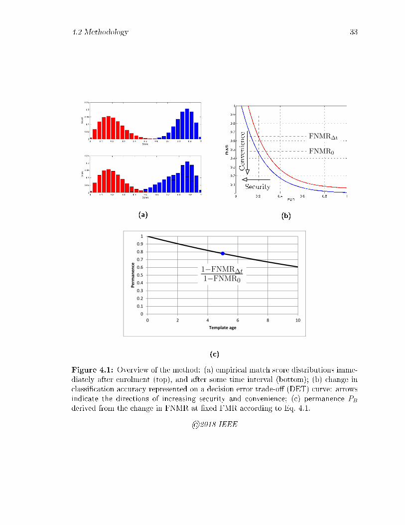
4.2 Methodology 33
(a)
FNMR0
FNMR∆t
Security
Convenience
(b)
0
0.1
0.2
0.3
0.4
0.5
0.6
0.7
0.8
0.9
1
0 2 4 6 8 10
Pe
rma
ne
nce
Template age
1−FNMR∆t1−FNMR0
(c)
Figure 4.1: Overview of the method: (a) empirical match score distributions imme-diately after enrolment (top), and after some time interval (bottom); (b) change inclassi�cation accuracy represented on a decision error trade-o� (DET) curve: arrowsindicate the directions of increasing security and convenience; (c) permanence PB
derived from the change in FNMR at �xed FMR according to Eq. 4.1.
©2018 IEEE
4.2 Methodology 34
In the pathological case where FNMR∆t < FNMR0, PB will be greater than 1.
4.2.2 Robust calculation
Given the above de�nition, it would appear relatively straightforward to calculate
biometric permanence from a set of repeated biometric captures. Unfortunately,
robust calculation of PB is complicated. Primarily, the issue is that the e�ects of
interest (small changes in the biometric features) occur in the context of many other
changes which are di�cult to control experimentally.
For example, in a longitudinal study over several years, there are changes in:
� weather: tests at di�erent times of the year expose subjects to � not yet well un-
derstood � physiological changes which a�ect biometric performance (e.g. levels
of skin dryness) [71].
� test administrators: over a period of several years there is inevitably some turn-
over in test sta�. Not all sta� are equally well trained. Some will be more
attentive in ensuring proper positioning and placement during biometric tests
than others [5].
� test administrator training: Even it it were possible to eliminate turn-over of
sta�, the training level of test sta� will adapt over time as they become more
familiar with the procedure.
� ageing of the biometric sensors: Biometric sensors are typically built of con-
sumer grade electronics and not intended for many years of useful life. Degra-
dation of some components in the sensors (e.g. lighting) can occur.
We address these issues with the matched delta methodology proposed in this section.
In overview, match score data are used to estimate the visit-speci�c factors (which
incorporate the variability above) and to separate them from the changes in match
4.2 Methodology 35
scores caused by template ageing e�ects. These visit-speci�c factors may then be
removed, leaving only the e�ect of template ageing.
Since we collect both enrolment templates and veri�cation images during each
visit, we can match all of the enrolment templates against all of the veri�cation images
and then visualize the available single-�nger match transactions as an N ×N matrix
(N the number of visits in the study) in which the upper triangle elements are the
`forward time' matches and the lower triangle are the `reverse time' matches. Along
the diagonal are the baseline (∆t = 0) scores in which each �nger image is matched
against a template taken only a few minutes before, i.e. at ∆t = 0. The essence of our
proposed methodology is that we can substantially remove the per-visit score biases
by looking at the di�erence in scores between a suitably chosen combination of visits
and the corresponding baseline visits, and applying these to a composite distribution
of the averaged baseline scores.
Our �matched delta� methodology is motivated by a simple additive model for
the measurement errors in the similarity scores. In the following section, a biometric
presentation refers to a single, �xed resolution, uncompressed bitmapped image of
a �ngerprint, while a template refers to a record of �ngerprint minutiae types and
locations extracted during subject enrolment, as described in [37, 38]. We assume
there is some true score sjinm between biometric presentation j in the nth veri�cation
visit, and a template i from the mth enrolment visit. In the context of �ngerprints,
i and j index a speci�c �nger of a speci�c subject; j = i therefore correspond to
genuine matches, and j = i to imposter matches. Then we postulate the following
error terms:
� a pair of visit biases am, bn representing systematic di�erences in the conditions
of the data collections such as operator training, subject acclimation, humidity
and so on;
� a stochastic term W ji representing the natural variability between repeated
4.2 Methodology 36
presentations of the same biometric.
Without loss of generality we can choose theW ji to be zero-mean. In our protocol,
we collect six images (in two contiguous veri�cation attempts, each consisting of three
presentations) and their averaged scores may then be modelled as
sjinm = sjinm + am + bn +Wji
(4.2)
This presentation averaging step is not essential to the methodology that follows;
however it is expected to reduce the variance of the stochastic error term. We then
observe that, in our experimental protocol, both enrolment templates and veri�cation
images are obtained from the same subject cohort at each visit. This allows us to
evaluate the average di�erence, forward and backward in time, between the match
score of biometric presentation j against template i with template age |∆tnm|, relative
to the average score at ∆tnn = ∆tmm = 0, as
∆sjinm (am, bn,Wij; ∆tij) =1
2
(sjinm + sjimn − sjimm − sjinn
)=
1
2
(sjimn + am + bn +W
ji
0
−sjimm − am − bm −Wji
1
+sjinm + an + bm +Wji
2
−sjinn − an − bn −Wji
3
)
where the Wji
k are assumed i.i.d. variables with the distribution of Wji, i.e.
∆sjinm (Wij; ∆tij) =1
2
{(sjinm + sjimn
)−(sjimm + sjinn
)+
3∑k=0
(−1)kWji
k
}(4.3)
in which it is seen that the bias terms have been eliminated, leaving just the averages
4.2 Methodology 37
of the forward and backward true scores and the baseline ∆t = 0 scores for the
corresponding visits. Meanwhile the stochastic terms, being uncorrelated, should add
on an RMS basis such that the variance of presentation-averaged scores over �ngers
i, j adds as
var
(1
2
3∑k=0
(−1)kWji
k
)= var
(W
ji
k
)(4.4)
leaving the signal-to-noise ratio of the measurement e�ectively unchanged1. The
various noise averaging steps may be summarized as:
W jik
over
presentations−−−−−−−−−−→ Wji
k
over
forward-
backward
visits−−−−−−−−−−→ 1
2
3∑k=0
(−1)kWji
k
4.2.3 Visit aggregation
A pervasive di�culty in the evaluation of biometric match performance is the inherent
class imbalance. That is, for a set ofK subject �nger presentations, we haveK(K−1)
imposter match scores but only K genuine match scores. This means that the genuine
match score distributions tend to be less well de�ned than those of the imposter
scores. In the context of the permanence measure Equation 4.1, this means that
while it is relatively straightforward to interpolate the threshold corresponding to a
chosen FMR, changes in the FNMR at that threshold may represent only a handful
of individual genuine matches.
One way to improve the imbalance would be to aggregate scores across multiple
devices in our study. Unfortunately however, while the API and biometric template
were standardized across device, vendors were free to chose their own scoring schemes
- which are hence largely incompatible. In order to improve the estimation, it was
1We have four i.i.d. random variables and we are subtracting two of them from the other two:the means subtract (to zero) but the variances add because the variance of −W is the same as thevariance of W .
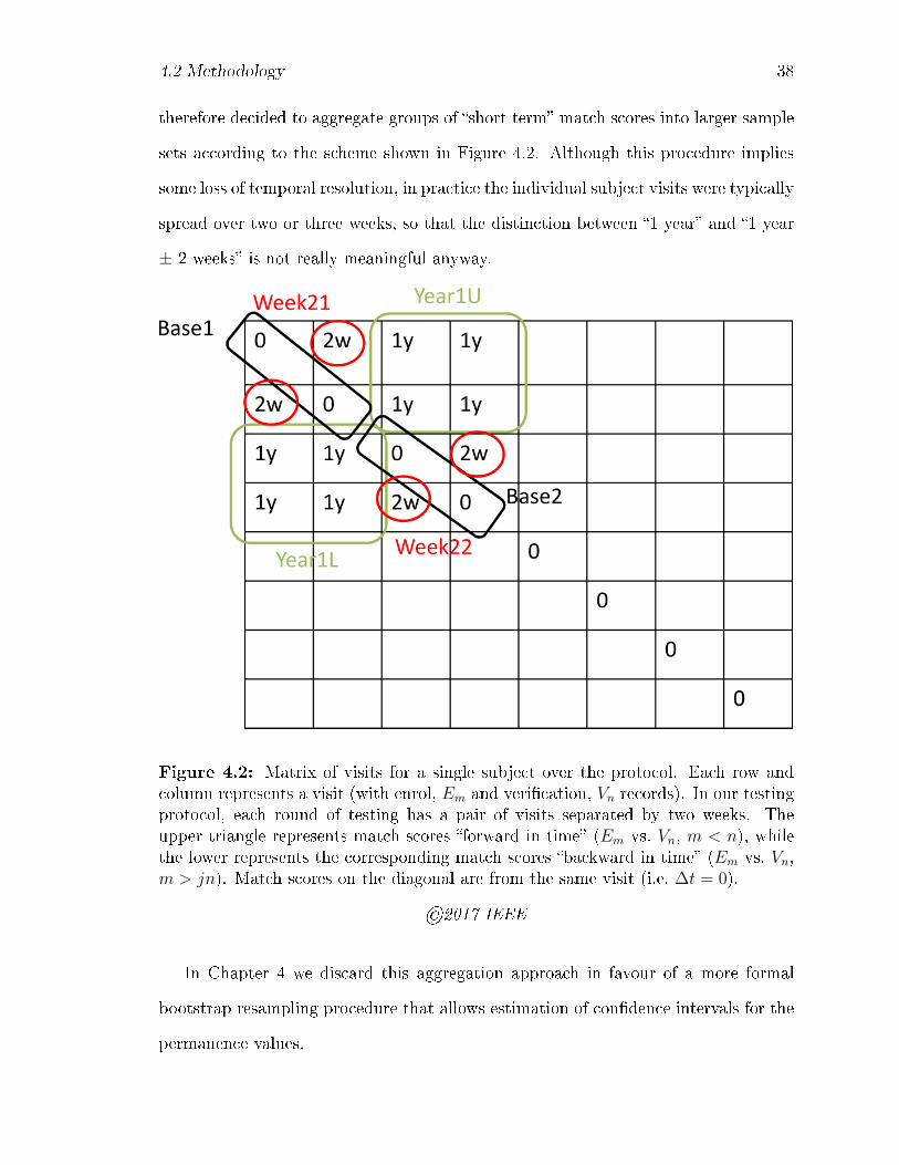
4.2 Methodology 38
therefore decided to aggregate groups of �short term� match scores into larger sample
sets according to the scheme shown in Figure 4.2. Although this procedure implies
some loss of temporal resolution, in practice the individual subject visits were typically
spread over two or three weeks, so that the distinction between �1 year� and �1 year
± 2 weeks� is not really meaningful anyway.
Figure 4.2: Matrix of visits for a single subject over the protocol. Each row andcolumn represents a visit (with enrol, Em and veri�cation, Vn records). In our testingprotocol, each round of testing has a pair of visits separated by two weeks. Theupper triangle represents match scores �forward in time� (Em vs. Vn, m < n), whilethe lower represents the corresponding match scores �backward in time� (Em vs. Vn,m > jn). Match scores on the diagonal are from the same visit (i.e. ∆t = 0).
©2017 IEEE
In Chapter 4 we discard this aggregation approach in favour of a more formal
bootstrap resampling procedure that allows estimation of con�dence intervals for the
permanence values.
4.3 Simulation 39
4.3 Simulation
We have de�ned biometric permanence, PB using, �rst, a model based on veri�cation
calculations alone (�reference methodology�, the value calculated this way is PB,R);
and next, a �matched delta methodology� (PB,M) in which visit variability is modelled
and removed by calculating the shift in the genuine distribution. Our expectations
are:
� In the absence of visit-to-visit variability, PB,M is an unbiased estimate of PB,R.
� PB,M is a lower variance estimator of PB,R (since a single parameter is estimated
from data before the DET calculation, which is known to be noisy).
� In the presence of visit-to-visit variability, PB,M will show more plausible results
than PB,R.
We take as our starting point a pair of canonical distributions for the underlying
false and genuine match scores, where scores range between 0 and 1. In this work
we have chosen to model the imposter scores via a simple Rayleigh distribution, and
the genuine scores via a ��ipped� Rayleigh distribution (Appendix D). In suitably
normalized form the probability densities become
pI(s) =s
β2I
e−s2/2β2I ; s ≥ 0 (4.5a)
pG(s) =1− s
β2G
e−(1−s)2/2β2G ; s ≤ 1 (4.5b)
where the scale parameters βI,G are related to the mean scores by µI = βI
√π2and
µG = 1− βG
√π2.
To model the sequence of enrolment-veri�cation visits, we then make two assump-
tions, namely
� The imposter distribution remains constant over time. Since the imposter dis-
4.3 Simulation 40
tribution represents non-matched samples, it will not be signi�cantly sensitive
to changes due to elapsed time. This is roughly equivalent to the assertion
that for any pair of non-identical �ngers whose match score is improved by
some mechanism, there is another pair whose match score is correspondingly
reduced.
� With each visit k we can associate a pair of systematic biases ak, bk (for enrol-
ment and veri�cation, respectively) that a�ect all presentations equally. We then
model the e�ect of a match score between a veri�cation presentation from visit
n against a template recorded in visit m as a shift in the genuine distribution
equal to (am + bn)
We then model the template ageing as a further, time-dependent, shift of the
genuine distribution. In this work we choose a simple time-symmetric assumption,
namely δ(∆t) = −α(1 − exp(−κ|∆t|)) i.e. a term that asymptotically approaches
δ = −α with time-constant 1/κ.
To each variate generated according to Eq. 4.5 we apply an additional zero-mean
Gaussian noise term W ji to represent the natural variation in match score over re-
peated presentations of the same �nger against the same template (e�ectively a kind
of `measurement noise').
4.3.1 Simulation of a single sequence of visits
To make a baseline qualitative evaluation of the e�cacy of our method in removing the
experimental biases, we constructed a single realization of a sequence of eight visits,
with bias values ak, bk taken from a Gaussian distribution with standard deviation
0.025. We then generated canonical sample distributions according to Eq. 4.5 for each
of two �ngers for a sample size of 17500 subjects
with µI = 0.2 and µG = 0.85 for each �nger. Next, for each of the 8 × 8 = 64

4.3 Simulation 41
enrol-verify visit combinations, we modify the �nger scores according to:
sj,in,m(∆t) = s0 + am + bn − α(1− exp(−κ|∆t|)) (4.6)
Finally, we synthesize six independent presentations of each �nger by adding a zero-
mean Gaussian noise term with variance σ2 = w2/6: this scaling is a convenience,
so that we can identify w2 with the sample variance of the presentation-averaged
experimental scores. We then processed the scores in two ways: (i) a simple direct
calculation according to Section 4.2.1; and (ii) our matched delta method as described
in Section 4.2.2.
We ran the simulation with three scenarios: �rst, with no visit biases (bn =
am = 0); second with bias in the creation of enrol templates only (bn = 0; am = 0);
and third with bias in both enrol template creation and veri�cation presentation
(bn = 0, am = 0). Results of these simulations are illustrated in Figure 4.3: each sub-
�gure shows PB (vertical axis) versus elapsed time (horizontal axis) in weeks between
enrolment and veri�cation. The {ON,OFF} status of parameters a (enrolment) and b
(veri�cation) represents whether the corresponding biases are simulated or not. Thus
�a:ON b:ON� indicates simulation of both enrolment and veri�cation biases. w is the
standard deviation of simulated presentation noise. The value of the presentation-
averaged sample standard deviation w was varied in the range 0 to 0.075 units and
the ageing parameters were α = 0.1 unit and κ = 0.01 week−1. The reference FMR
for the permanence calculation was 0.001 (0.1%).
Taken together, the visit bias terms and ageing correspond to a modi�cation
(1 − s) → (1 − am − bn − δ(t) − s) in the genuine score distribution of Eq. 4.5.
The densities then become convolved with the Gaussian density � one can show
(Appendix D) that the resulting tail integrals for the FMR and FNMR at some
4.3 Simulation 42
threshold score θ become:
FMR(θ) =βI
β′I
e−θ2/2β′2I (4.7a)
FNMR(θ;m,n; t) =βG
β′G
e−(χ(t;m,n)−θ)2/2β′2G (4.7b)
where β′2I,G = β2
I,G + σ2I,G (with σ2
I,G being the variances of the imposter and genuine
presentation noise terms respectively) and
χ(t;m,n) = 1− am − bn − δ(t) (4.8)
represents the mean degradation in genuine match score due to the per-visit biases
and template ageing. The solid black curves in Figure 4.3 correspond to Eq. 4.7 , 4.8
with am = bn = 0 i.e. they represent the `ideal' (unbiased) ageing behaviour that
would be observed due to presentation noise only: the deviation from this curve can
be interpreted as the residual e�ect of bias that is not removed by the technique.
4.3.2 Simulation of an ensemble of visit sequences
Over an ensemble of experiments (that is, sequences of enrol-verify visits) with exper-
imental biases taken independently from some zero-mean distribution(s), one would
like to show that the mean of the reference permanence measure (Eq. 4.1) does indeed
converge to the value obtained by our new technique. Accordingly we ran the same
procedure up to 180 times to simulate multiple independent realizations of our ex-
periment. At intervals of 5 simulated experiments we calculated the mean deviation
(across time di�erences ∆tnm) between the permanence calculated according to our
method (Section 4.2.2) and reference method (Section 4.2.1) (Figure 4.4).
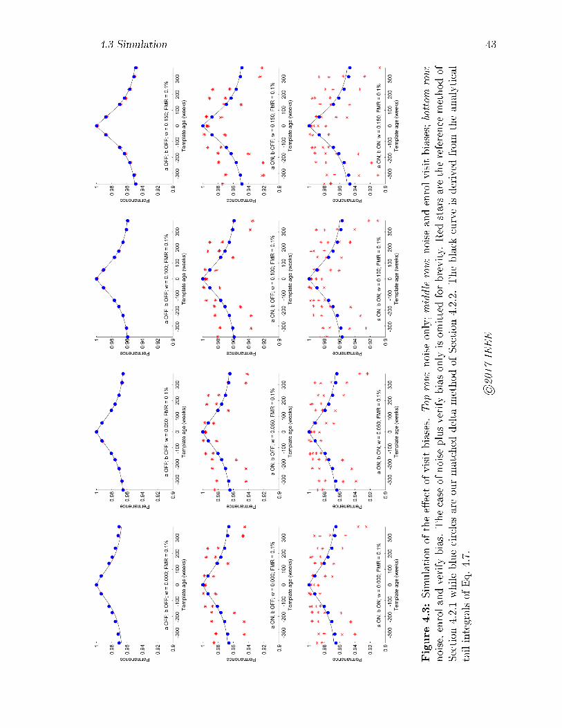
4.3 Simulation 43
Figure
4.3:Simulation
ofthee�ectof
visitbiases.
Top
row:noise
only;middlerow:noise
andenrolvisitbiases;bottom
row:
noise,enrolandverify
bias.Thecase
ofnoise
plusverify
biasonly
isom
ittedforbrevity.
Red
starsarethereference
methodof
Section
4.2.1whilebluecirclesareourmatched
delta
methodof
Section
4.2.2.
Theblack
curveisderived
from
theanalytical
tailintegralsof
Eq.4.7.
©2017
IEEE
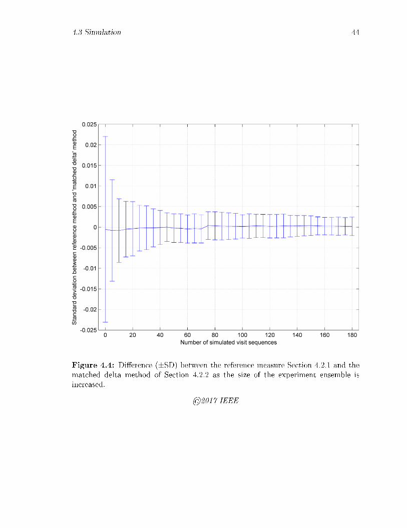
4.3 Simulation 44
Figure 4.4: Di�erence (±SD) between the reference measure Section 4.2.1 and thematched delta method of Section 4.2.2 as the size of the experiment ensemble isincreased.
©2017 IEEE
4.4 Discussion 45
4.4 Discussion
We have developed and de�ned a measure of template ageing which we call biometric
permanence PB, based on the change in FNMR (at a given FMR) between the tem-
plate ageing interval under test, and a short-time test. While intuitive, this de�nition
of PB is practically di�cult to apply to estimate small changes in permanence in a
longitudinal study subject to experimental error and visit-to-visit systematic biases.
To address this issue, we have introduced the matched delta method. Comparisons
of these methods were performed using simulated data, and it was determined that
the new method showed dramatically reduced sensitivity to systematic biases. Sim-
ulations were designed to evaluate two aspects of the proposed robust calculation
method in comparison to the calculation of PB from Eq. 4.1. First, simulations test
the �rst and second order statistical properties (i.e. bias and variance); and, second,
the sensitivity of the methods to visit-to-visit biases.
Figure 4.3 compares the two methods to the analytical values (Eq. 4.7). For two
di�erent values of presentation noise (columns), the presence or absence of visit biases
is evaluated. A single sample of visit biases is evaluated in each case; multiple values
at a single time interval indicate di�erent ways in which the given time o�set can
be calculated. Without visit biases, the methods perform similarly, while their pres-
ence dramatically impacts the values calculated using Eq. 4.1. Meanwhile Figure 4.4
investigates the statistical properties of the methods. As sample number increases,
the variance decreases and bias between methods decreases towards zero, as expected
from our analytical model.
Chapter 5
Characterization of biometric
template ageing in a multi-year,
multi-vendor longitudinal �ngerprint
matching study
In Chapter 4 we outlined a method for evaluating the permanence of a set of bio-
metric templates, based on a simple phenomenological model for confounding factors
resulting from changes in physical environment and acclimation.
The goal of this chapter is to characterize template ageing in the �ngerprint modal-
ity, for a number of commercially-available �ngerprint sensor devices and technologies,
and to understand its impact on the deployment and operation of �ngerprint-based
IDMSs.
In Section 5.2, results are presented for each of the devices. Finally, in Section 5.3
we attempt to justify, through further data analysis, the key assumptions underlying
the methodology.
46
5.1 Methodology 47
5.1 Methodology
The methodology follows that of the previous chapter, with the following exception.
In Chapter 4, we noted that aside from the visit-to-visit confounding factors such
as variations in environmental conditions, operator training and subject acclimation,
the chief di�culty in estimating template permanence according to our de�nition of
Equation 4.1 is the relatively poor de�nition of the empirical genuine score distribu-
tions. This in turn results from the inherent class imbalance i.e. that whereas the
number of imposter matches increases quadratically with the number of individuals
in the study, that of the genuine scores only increases linearly. For the simulated
study of that chapter, we implemented a �visit aggregation� scheme to boost the sizes
of the genuine match score sets. Here we develop a more robust scheme based on
bootstrap resampling [56].
As in our earlier procedure, the averaged �matched deltas� ∆sjinm from Equation 4.3
are averaged again across a particular pair of enrolment and veri�cation visits m,n
to give mean genuine and imposter score o�sets ∆sGnm and ∆sInm for the chosen visit
pair n,m. We then aggregate the corresponding zero-time genuine and imposter
scores {siikk}, {sj =ikk }; k ∈ 1 . . . N and use these aggregate distributions shifted by the
respective mean o�sets ∆sGnm, ∆sInm to evaluate PB according to Equation 4.1 at
time interval ∆tmn. In order to perform the bootstrap resampling, we arrange the
aggregate genuine and imposter scores into a vector(siikk, s
j =ikk
)along with a vector
of class labels (1nG,OnI
) where nG, nI are the genuine and imposter class sizes in
the sample. The bootstrap procedure was then developed in a number of stages, as
follows.
The initial implementation consisted of a simple N -fold resampling, with replace-
ment, of the entire labelled datasets i.e.
� select nTot = nG + nI scores, randomly with replacement
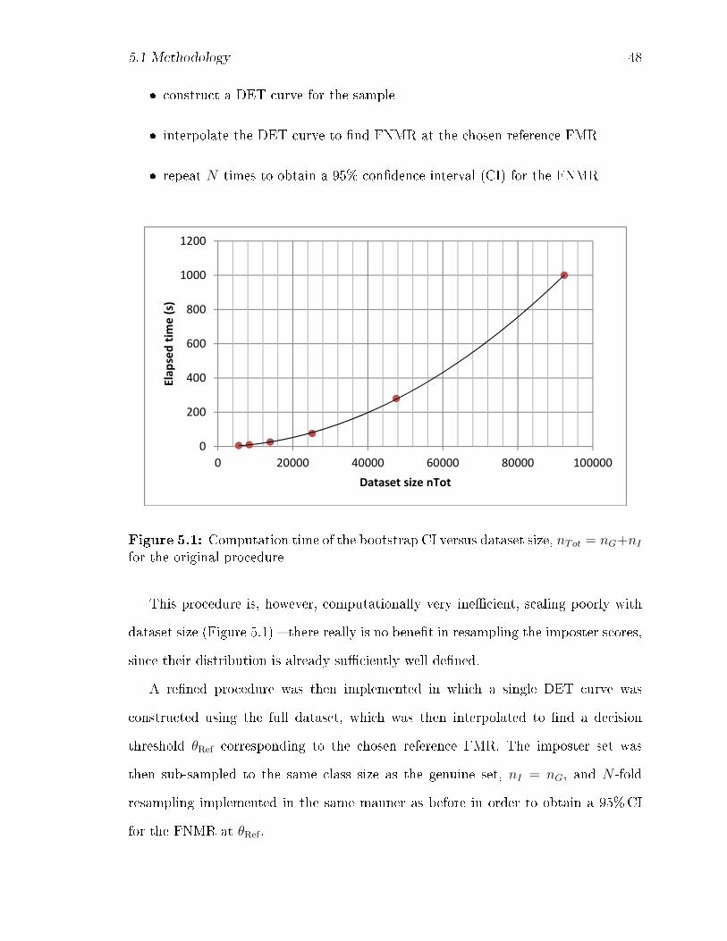
5.1 Methodology 48
� construct a DET curve for the sample
� interpolate the DET curve to �nd FNMR at the chosen reference FMR
� repeat N times to obtain a 95% con�dence interval (CI) for the FNMR
0
200
400
600
800
1000
1200
0 20000 40000 60000 80000 100000
Ela
pse
d t
ime
(s)
Dataset size nTot
Figure 5.1: Computation time of the bootstrap CI versus dataset size, nTot = nG+nI
for the original procedure
This procedure is, however, computationally very ine�cient, scaling poorly with
dataset size (Figure 5.1) � there really is no bene�t in resampling the imposter scores,
since their distribution is already su�ciently well de�ned.
A re�ned procedure was then implemented in which a single DET curve was
constructed using the full dataset, which was then interpolated to �nd a decision
threshold θRef corresponding to the chosen reference FMR. The imposter set was
then sub-sampled to the same class size as the genuine set, nI = nG, and N -fold
resampling implemented in the same manner as before in order to obtain a 95%CI
for the FNMR at θRef .
5.1 Methodology 49
Although more e�cient, a signi�cant �aw remains in that the construction leads
to a con�dence interval for the FNMR, rather than for the permanence measure, PB.
To address this, an improved bootstrap procedure was developed. First, Equation 4.1
was re-cast in terms of true match rate (TMR) as
PB(∆t,FMR) =TMR∆t
TMR0
(5.1)
Next we noted that, since an o�set ∆SIto the imposter distribution is exactly
equivalent to a shift in the threshold θ → θ + ∆SIfor the chosen FMR, while an
o�set to the genuine distribution is similarly equivalent to a shift θ → θ −∆SG, we
just need to evaluate 1 − FNMR (or, equivalently, the true match rate TMR) at a
set of thresholds θnm = θ0 +∆sInm −∆sGnm (Fig. 5.2). In fact, since we de�ned PB as
a ratio, it su�ces to work with the raw genuine score counts i.e. the permanence is
estimated for each bootstrap sample as
PB(∆tnm) =
{siikk : siikk > θ0 +∆sInm −∆sGnm}
{siikk : siikk > θ0}
(5.2)
evaluated for each enrolment-veri�cation visit pair n,m, where |C| denotes the car-
dinality of C.
The procedure was developed in MATLAB using the perfcurve function from the
Statistics and Machine Learning Toolbox, with the permanence measure of Equa-
tion 5.1 as a parametrized bootfun. The resampling was class-weighted in inverse
proportion to the original class sizes nG and nI in order to remove class imbalance.
The interested reader is referred to the MATLAB code in Appendix C for details
of the implementation.
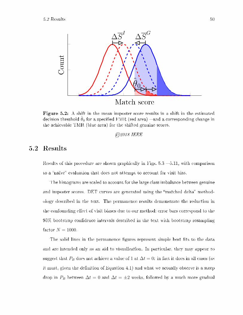
5.2 Results 50
∆SI
∆SG
θ0
Match score
Count
Figure 5.2: A shift in the mean imposter score results in a shift in the estimateddecision threshold θ0 for a speci�ed FMR (red area) � and a corresponding change inthe achievable TMR (blue area) for the shifted genuine scores.
©2018 IEEE
5.2 Results
Results of this procedure are shown graphically in Figs. 5.3 � 5.11, with comparison
to a �naïve� evaluation that does not attempt to account for visit bias.
The histograms are scaled to account for the large class imbalance between genuine
and imposter scores. DET curves are generated using the �matched delta� method-
ology described in the text. The permanence results demonstrate the reduction in
the confounding e�ect of visit biases due to our method; error bars correspond to the
95% bootstrap con�dence intervals described in the text with bootstrap resampling
factor N = 1000.
The solid lines in the permanence �gures represent simple best �ts to the data
and are intended only as an aid to visualization. In particular, they may appear to
suggest that PB does not achieve a value of 1 at ∆t = 0: in fact it does in all cases (as
it must, given the de�nition of Equation 4.1) and what we actually observe is a steep
drop in PB between ∆t = 0 and ∆t = ±2 weeks, followed by a much more gradual
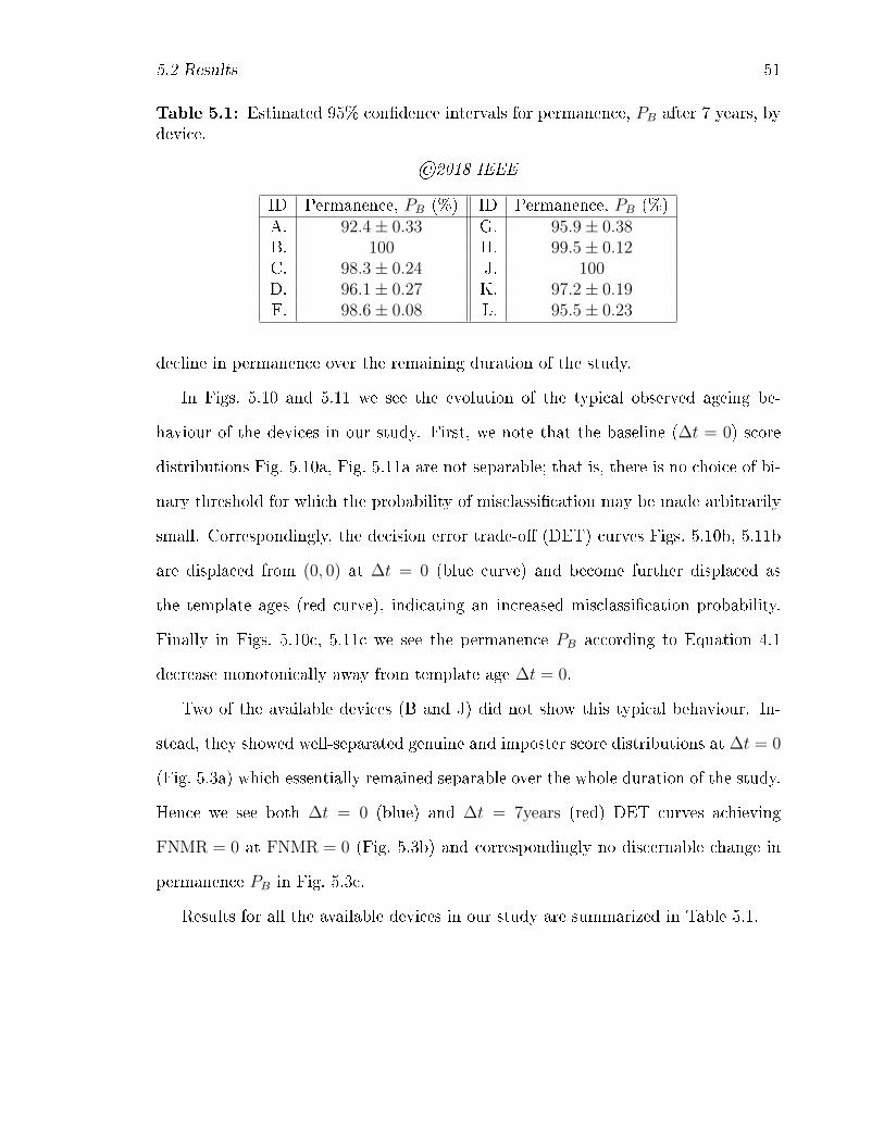
5.2 Results 51
Table 5.1: Estimated 95% con�dence intervals for permanence, PB after 7 years, bydevice.
©2018 IEEE
ID Permanence, PB (%) ID Permanence, PB (%)A. 92.4± 0.33 G. 95.9± 0.38B. 100 H. 99.5± 0.12C. 98.3± 0.24 J. 100D. 96.1± 0.27 K. 97.2± 0.19F. 98.6± 0.08 L. 95.5± 0.23
decline in permanence over the remaining duration of the study.
In Figs. 5.10 and 5.11 we see the evolution of the typical observed ageing be-
haviour of the devices in our study. First, we note that the baseline (∆t = 0) score
distributions Fig. 5.10a, Fig. 5.11a are not separable; that is, there is no choice of bi-
nary threshold for which the probability of misclassi�cation may be made arbitrarily
small. Correspondingly, the decision error trade-o� (DET) curves Figs. 5.10b, 5.11b
are displaced from (0, 0) at ∆t = 0 (blue curve) and become further displaced as
the template ages (red curve), indicating an increased misclassi�cation probability.
Finally in Figs. 5.10c, 5.11c we see the permanence PB according to Equation 4.1
decrease monotonically away from template age ∆t = 0.
Two of the available devices (B and J) did not show this typical behaviour. In-
stead, they showed well-separated genuine and imposter score distributions at ∆t = 0
(Fig. 5.3a) which essentially remained separable over the whole duration of the study.
Hence we see both ∆t = 0 (blue) and ∆t = 7years (red) DET curves achieving
FNMR = 0 at FNMR = 0 (Fig. 5.3b) and correspondingly no discernable change in
permanence PB in Fig. 5.3c.
Results for all the available devices in our study are summarized in Table 5.1.
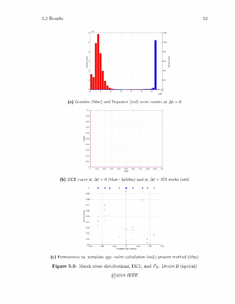
5.2 Results 52
0 1 2 3 4 5 6 7
10 4
0
1
2
3
4
5
6
Impo
ster
cou
nt
10 4
0 1 2 3 4 5 6 7
10 4
0
200
400
600
800
1000
1200
Gen
uine
cou
nt
(a) Genuine (blue) and Imposter (red) score counts at ∆t = 0
0 0.01 0.02 0.03 0.04 0.05 0.06 0.07 0.08 0.09 0.1
FMR
0
0.01
0.02
0.03
0.04
0.05
0.06
0.07
0.08
0.09
0.1
FN
MR
(b) DET curve at ∆t = 0 (blue - hidden) and at ∆t = 373 weeks (red)
(c) Permanence vs. template age: naïve calculation (red); present method (blue)
Figure 5.3: Match score distributions, DET, and PB: DeviceB (optical)
©2018 IEEE
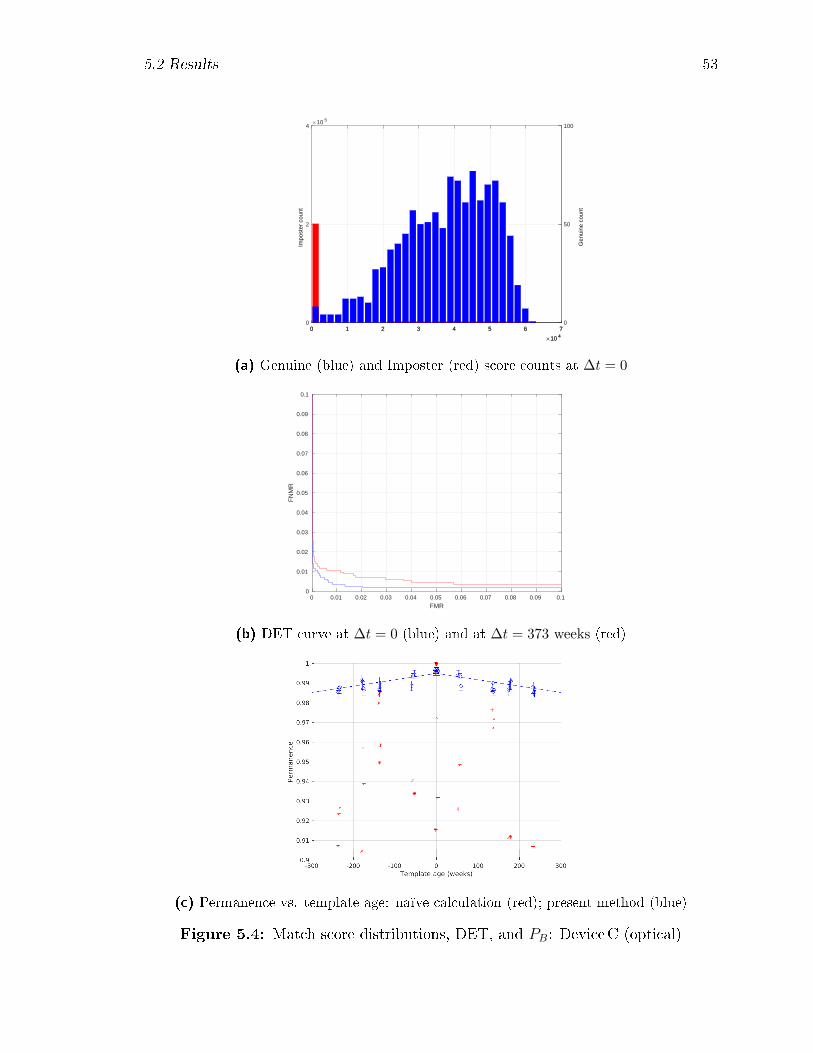
5.2 Results 53
0 1 2 3 4 5 6 7
10 4
0
2
4
Impo
ster
cou
nt
10 5
0 1 2 3 4 5 6 7
10 4
0
50
100
Gen
uine
cou
nt
(a) Genuine (blue) and Imposter (red) score counts at ∆t = 0
0 0.01 0.02 0.03 0.04 0.05 0.06 0.07 0.08 0.09 0.1
FMR
0
0.01
0.02
0.03
0.04
0.05
0.06
0.07
0.08
0.09
0.1
FN
MR
(b) DET curve at ∆t = 0 (blue) and at ∆t = 373 weeks (red)
(c) Permanence vs. template age: naïve calculation (red); present method (blue)
Figure 5.4: Match score distributions, DET, and PB: DeviceC (optical)

5.2 Results 54
0 1 2 3 4 5 6 7
10 4
0
1
2
Impo
ster
cou
nt
10 5
0 1 2 3 4 5 6 7
10 4
0
50
100
Gen
uine
cou
nt
(a) Genuine (blue) and Imposter (red) score counts at ∆t = 0
0 0.01 0.02 0.03 0.04 0.05 0.06 0.07 0.08 0.09 0.1
FMR
0
0.01
0.02
0.03
0.04
0.05
0.06
0.07
0.08
0.09
0.1
FN
MR
(b) DET curve at ∆t = 0 (blue) and at ∆t = 373 weeks (red)
(c) Permanence vs. template age: naïve calculation (red); present method (blue)
Figure 5.5: Match score distributions, DET, and PB: DeviceD (optical)
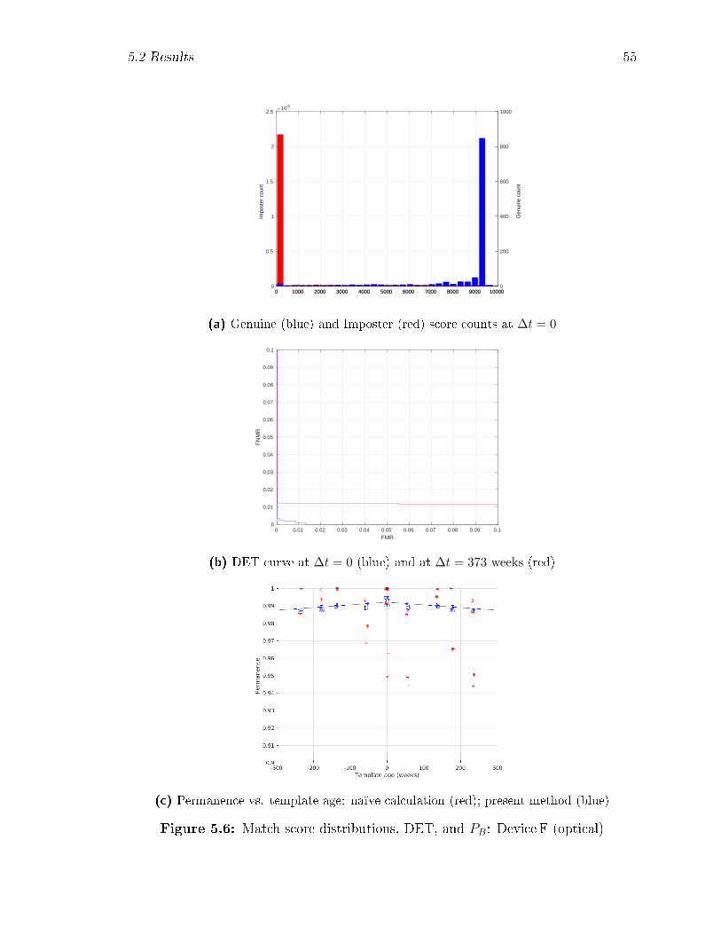
5.2 Results 55
0 1000 2000 3000 4000 5000 6000 7000 8000 9000 100000
0.5
1
1.5
2
2.5
Impo
ster
cou
nt
10 5
0 1000 2000 3000 4000 5000 6000 7000 8000 9000 100000
200
400
600
800
1000
Gen
uine
cou
nt
(a) Genuine (blue) and Imposter (red) score counts at ∆t = 0
0 0.01 0.02 0.03 0.04 0.05 0.06 0.07 0.08 0.09 0.1
FMR
0
0.01
0.02
0.03
0.04
0.05
0.06
0.07
0.08
0.09
0.1
FN
MR
(b) DET curve at ∆t = 0 (blue) and at ∆t = 373 weeks (red)
(c) Permanence vs. template age: naïve calculation (red); present method (blue)
Figure 5.6: Match score distributions, DET, and PB: Device F (optical)
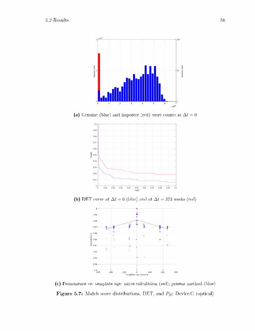
5.2 Results 56
0 1 2 3 4 5 6 7
10 4
0
1
2
Impo
ster
cou
nt
10 5
0 1 2 3 4 5 6 7
10 4
0
50
100
Gen
uine
cou
nt
(a) Genuine (blue) and Imposter (red) score counts at ∆t = 0
0 0.01 0.02 0.03 0.04 0.05 0.06 0.07 0.08 0.09 0.1
FMR
0
0.01
0.02
0.03
0.04
0.05
0.06
0.07
0.08
0.09
0.1
FN
MR
(b) DET curve at ∆t = 0 (blue) and at ∆t = 373 weeks (red)
(c) Permanence vs. template age: naïve calculation (red); present method (blue)
Figure 5.7: Match score distributions, DET, and PB: DeviceG (optical)
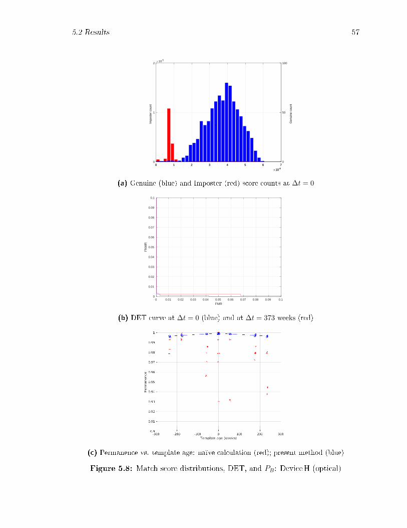
5.2 Results 57
0 1 2 3 4 5 6 7
10 4
0
1
2
Impo
ster
cou
nt
10 5
0 1 2 3 4 5 6 7
10 4
0
50
100
Gen
uine
cou
nt
(a) Genuine (blue) and Imposter (red) score counts at ∆t = 0
0 0.01 0.02 0.03 0.04 0.05 0.06 0.07 0.08 0.09 0.1
FMR
0
0.01
0.02
0.03
0.04
0.05
0.06
0.07
0.08
0.09
0.1
FN
MR
(b) DET curve at ∆t = 0 (blue) and at ∆t = 373 weeks (red)
(c) Permanence vs. template age: naïve calculation (red); present method (blue)
Figure 5.8: Match score distributions, DET, and PB: DeviceH (optical)
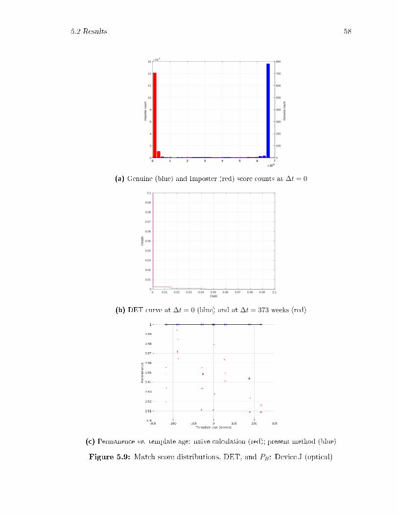
5.2 Results 58
0 1 2 3 4 5 6 7
10 4
0
2
4
6
8
10
12
14
16
Impo
ster
cou
nt
10 4
0 1 2 3 4 5 6 7
10 4
0
100
200
300
400
500
600
700
800
Gen
uine
cou
nt
(a) Genuine (blue) and Imposter (red) score counts at ∆t = 0
0 0.01 0.02 0.03 0.04 0.05 0.06 0.07 0.08 0.09 0.1
FMR
0
0.01
0.02
0.03
0.04
0.05
0.06
0.07
0.08
0.09
0.1
FN
MR
(b) DET curve at ∆t = 0 (blue) and at ∆t = 373 weeks (red)
(c) Permanence vs. template age: naïve calculation (red); present method (blue)
Figure 5.9: Match score distributions, DET, and PB: Device J (optical)

5.2 Results 59
0 1 2 3 4 5 6 7
10 4
0
1
2
Impo
ster
cou
nt
10 5
0 1 2 3 4 5 6 7
10 4
0
100
200
Gen
uine
cou
nt
(a) Genuine (blue) and Imposter (red) score counts at ∆t = 0
0 0.01 0.02 0.03 0.04 0.05 0.06 0.07 0.08 0.09 0.1
FMR
0
0.01
0.02
0.03
0.04
0.05
0.06
0.07
0.08
0.09
0.1
FN
MR
(b) DET curve at ∆t = 0 (blue) and at ∆t = 373 weeks (red)
(c) Permanence vs. template age: naïve calculation (red); present method (blue)
Figure 5.10: Match score distributions, DET, and PB: DeviceK (optical)
©2018 IEEE
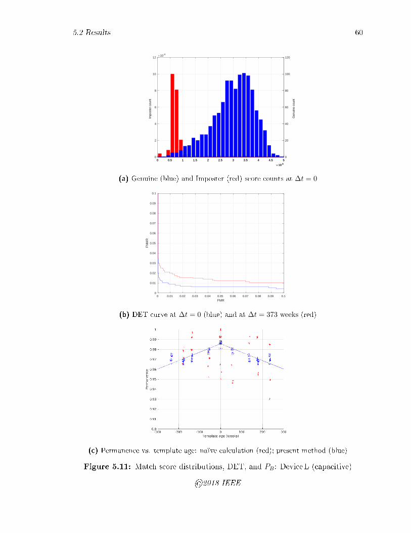
5.2 Results 60
0 0.5 1 1.5 2 2.5 3 3.5 4 4.5 5
10 4
0
2
4
6
8
10
12
Impo
ster
cou
nt
10 4
0 0.5 1 1.5 2 2.5 3 3.5 4 4.5 5
10 4
0
20
40
60
80
100
120
Gen
uine
cou
nt
(a) Genuine (blue) and Imposter (red) score counts at ∆t = 0
0 0.01 0.02 0.03 0.04 0.05 0.06 0.07 0.08 0.09 0.1
FMR
0
0.01
0.02
0.03
0.04
0.05
0.06
0.07
0.08
0.09
0.1
FN
MR
(b) DET curve at ∆t = 0 (blue) and at ∆t = 373 weeks (red)
(c) Permanence vs. template age: naïve calculation (red); present method (blue)
Figure 5.11: Match score distributions, DET, and PB: Device L (capacitive)
©2018 IEEE
5.3 Discussion 61
5.3 Discussion
The values of PB derived using the preceding methodology show one of two dis-
tinct characteristics: either monotonically decreasing over the course of the study,
or constant, depending on the speci�c device under test. These characteristics seem
intuitively reasonable when we consider the baseline (relative template age ∆tmn = 0)
genuine and imposter score distributions: those that are essentially separable at
∆tmn = 0 remain so for the duration of the study, while those whose genuine and
imposter scores overlap at ∆tmn = 0. In no case did we observe an increasing trend
in PB over time: in this respect, we believe that our methodology exhibits convergent
validity with respect to the recorded template ages.
A question that arises in this respect is whether the permanence estimates in
Table 5.1 may be used to identify �good� versus �bad� devices. Since our de�nition of
PB uses the day zero FNMR as a normalizing factor, the answer is generally `no': a
bad device that simply does not get much worse over time may still display high PB.
For the two devices that showed no change in permanence, the analysis is likely
a�ected by the large class imbalance inherent in such biometric comparisons. That is,
for a dataset of K distinct �ngers, there are of order K2 imposter matches but only K
genuine matches, which causes the tails of the genuine match score distributions to be
much less well de�ned than those of the imposter distributions. This in turn makes it
hard to estimate with con�dence the threshold at which to evaluate the corresponding
FNMR for the permanence calculation. While the bootstrapping procedure described
in 5.2 attempts to ameliorate this e�ect, if the empirical distributions are separable,
then no amount of re-sampling can guarantee that there will be a non-zero FNMR
at the chosen FMR. In this regard, a larger study size would have increased the
probability of observing ageing behaviour where present.
Since the majority (8 out of 10) devices did show a measurable reduction in
permanence over the 7 years, we believe we have observed template ageing over this
5.3 Discussion 62
time span. A time span of 7 years is broadly in line with common renewal intervals
of documents such as biometrically enabled passports (typically either 5 or 10 years),
and therefore should be of practical interest to the end users of such technologies. It
would be particularly interesting to extend the duration of the study to see whether
they eventually showed a similar trend in discriminability.
In the following sections we discuss some other aspects of the data, and their
potential impact upon the interpretation of our results.
5.3.1 Time symmetry of the match scores
A key assumption that allows us to substantially remove the visit-to-visit bias factors
is that the underlying �true� match scores are time-symmetric: that is, in the absence
of these factors, comparisons between a biometric enrolment obtained at time t1 and
a set of veri�cation presentations at later time t2, and between a biometric enrolment
obtained at time t2 and a set of veri�cation presentations at earlier time t1, have the
same expected match score. (`Expected' because there will still be presentation-to-
presentation variability, denoted by the W ij terms in our formalism.) The extent
to which this is the case will depend on the algorithm and implementation of the
similarity measures used: we might imagine that a simple degree-of-overlap measure
to be time-symmetric, whereas a more heuristic matcher might not be. For example,
consider the case in which the number of extractable �ngerprint minutiae decreases
with time, perhaps due to occupational injury or environmental damage; when applied
in the reverse time direction, a heuristic might consider the apparent increase in
minutiae count to be implausible. Unfortunately such implementation details were
not available for the devices in our study.
5.3 Discussion 63
5.3.2 Constancy of the imposter distributions
Intuitively, we might expect the imposter score distribution to be relatively insensitive
to template age, since factors that decrease the similarity between any given pair of
subject-�ngers may increase the similarity between other such imposter pairs.1However
this does not allow for gross di�erences in biometric presentation quality between dif-
ferent pairs of visits. We attempted to quantify the relative contributions of mean
changes in imposter scores and those of the genuine match scores as follows.
It is important here to distinguish between statistically signi�cant changes, and
changes of signi�cant e�ect size: since the imposter sample sizes ( ∼ K2, for a sample
of K distinct subject-�ngers) are approximately two orders of magnitude larger than
those of the genuine matches (∼ K, for the same set of subject-�ngers), it is almost
always possible to reject the null hypothesis that the imposter samples at ∆tnm come
from the same distribution as those at ∆tmm. First we de�ne a discriminability
measureQnm for a pair of visits n,m as the ratio of the di�erence in sample mean score
u between genuine and imposter presentations to the sum of their sample standard
deviations s
Qnm =uGnm − uI
nm
sGnm + sInm(5.3)
This measure is similar to the Mahalanobis distance familiar from linear discriminant
analysis (LDA); the form chosen here is widely used for characterizing the error
probability in a binary optical communication channel [23]. We then de�ne the visit-
averaged quantities
uG =1
NM
N∑ M∑uGnm sG =
1
NM
N∑ M∑sGnm (5.4)
uI =1
NM
N∑ M∑uInm sI =
1
NM
N∑ M∑sInm (5.5)
1This in fact was an assumption made in the simulations of Chapter 4.
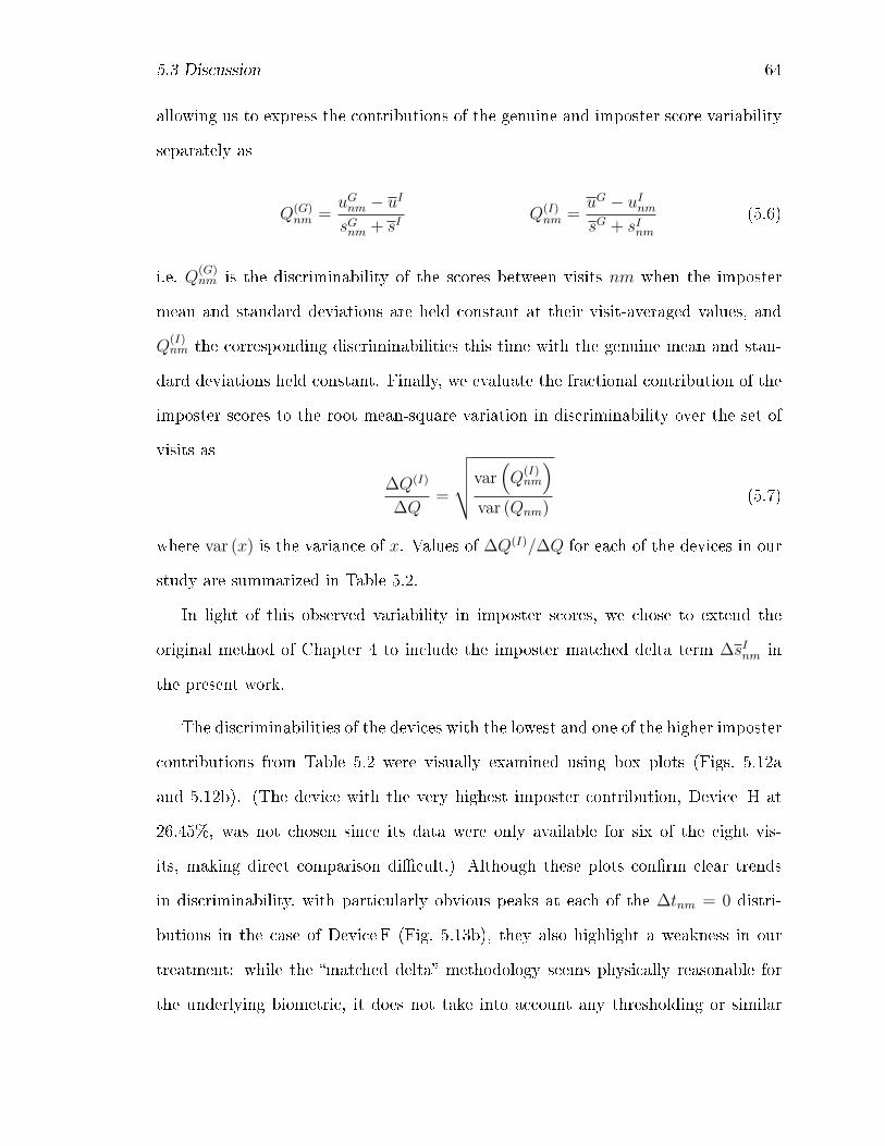
5.3 Discussion 64
allowing us to express the contributions of the genuine and imposter score variability
separately as
Q(G)nm =
uGnm − uI
sGnm + sIQ(I)
nm =uG − uI
nm
sG + sInm(5.6)
i.e. Q(G)nm is the discriminability of the scores between visits nm when the imposter
mean and standard deviations are held constant at their visit-averaged values, and
Q(I)nm the corresponding discriminabilities this time with the genuine mean and stan-
dard deviations held constant. Finally, we evaluate the fractional contribution of the
imposter scores to the root mean-square variation in discriminability over the set of
visits as
∆Q(I)
∆Q=
⌜⎷var(Q
(I)nm
)var (Qnm)
(5.7)
where var (x) is the variance of x. Values of ∆Q(I)/∆Q for each of the devices in our
study are summarized in Table 5.2.
In light of this observed variability in imposter scores, we chose to extend the
original method of Chapter 4 to include the imposter matched delta term ∆sInm in
the present work.
The discriminabilities of the devices with the lowest and one of the higher imposter
contributions from Table 5.2 were visually examined using box plots (Figs. 5.12a
and 5.12b). (The device with the very highest imposter contribution, Device H at
26.45%, was not chosen since its data were only available for six of the eight vis-
its, making direct comparison di�cult.) Although these plots con�rm clear trends
in discriminability, with particularly obvious peaks at each of the ∆tnm = 0 distri-
butions in the case of Device F (Fig. 5.13b), they also highlight a weakness in our
treatment: while the �matched delta� methodology seems physically reasonable for
the underlying biometric, it does not take into account any thresholding or similar

5.3 Discussion 65
Table 5.2: Relative e�ect of the imposter distributions to the RMS change in matchscore discriminability, by device.
©2018 IEEE
ID ∆Q(I)/∆Q (%) ID ∆Q(I)/∆Q (%)A. 0.40 G. 6.80B. 12.46 H. 26.45C. 7.40 J. 1.57D. 21.12 K. 1.68F. 0.07 L. 12.49
non-linear processing of the raw match scores. In particular, whereas the box plots
of Fig. 5.12a �t well to our assumption that the distributions change in their mean
value rather than their shape, those of Fig. 5.12b show distinct limiting behaviour in
the - processed - genuine distributions.
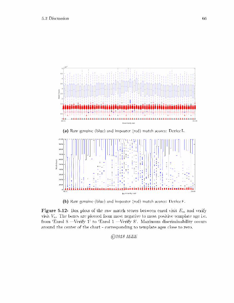
5.3 Discussion 66
E8-V1 E1-V8
Enrol-Verify visit
0
0.5
1
1.5
2
2.5
3
3.5
4
4.5
5
Mat
ch S
core
10 4
(a) Raw genuine (blue) and imposter (red) match scores: Device L.
(b) Raw genuine (blue) and imposter (red) match scores: Device F.
Figure 5.12: Box plots of the raw match scores between enrol visit Em and verifyvisit Vn. The boxes are plotted from most negative to most positive template age i.e.from `Enrol 8 � Verify 1' to `Enrol 1 � Verify 8'. Maximum discriminability occursaround the center of the chart - corresponding to template ages close to zero.
©2018 IEEE
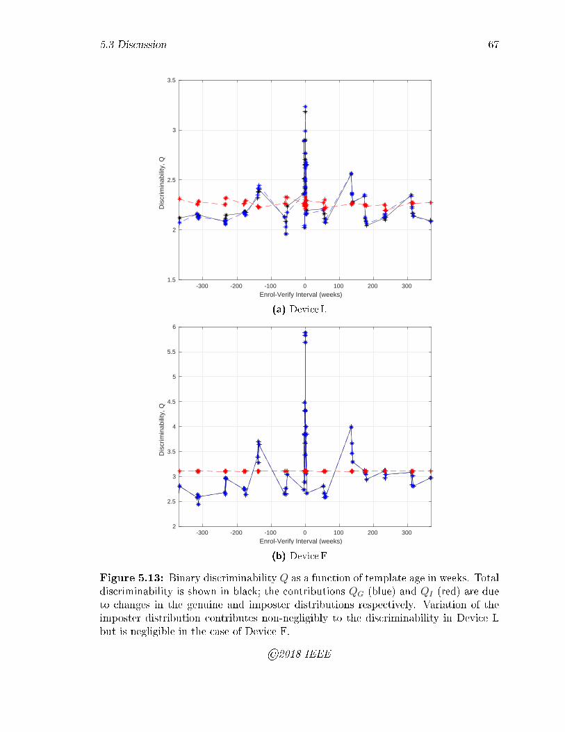
5.3 Discussion 67
-300 -200 -100 0 100 200 300
Enrol-Verify Interval (weeks)
1.5
2
2.5
3
3.5
Dis
crim
inab
ility
, Q
(a) Device L
-300 -200 -100 0 100 200 300
Enrol-Verify Interval (weeks)
2
2.5
3
3.5
4
4.5
5
5.5
6
Dis
crim
inab
ility
, Q
(b) Device F
Figure 5.13: Binary discriminability Q as a function of template age in weeks. Totaldiscriminability is shown in black; the contributions QG (blue) and QI (red) are dueto changes in the genuine and imposter distributions respectively. Variation of theimposter distribution contributes non-negligibly to the discriminability in Device Lbut is negligible in the case of Device F.
©2018 IEEE
5.4 Conclusion 68
5.4 Conclusion
We have elaborated a method to isolate and measure changes in biometric system
performance over time, using a metric which we call biometric permanence. The
method was applied to a dataset spanning several years, and template ageing accord-
ing to this metric was observed in 8 out of 10 available devices. We have discussed
the limits of validity of the underlying assumptions of the methodology, highlighting
some device-dependent characteristics of the match score distributions. Because of
these factors, it seems appropriate to consider template ageing to be a property of
a given biometric system as a whole, rather than a speci�c physiological mechanism
or biometric modality. In order to maintain system performance over life, we recom-
mend that system integrators take such template ageing behaviour into account � for
example, by implementing an in-service template update procedure, or a requirement
for periodic re-enrolment.
Chapter 6
Biometric quality and classi�cation
performance
In this chapter, we compare the available measures of biometric quality on a device-
by-device basis, �rst from the point of view of their assessed quality scores, and
then as predictors of classi�cation performance. The goal of the chapter is to un-
derstand the relationship between NFIQ-1 and NFIQ-2 scores (and, where available,
vendor-speci�c quality scores obtained during template enrolment), and the relation-
ship between these scores and the measured biometric performance - both in terms
of raw match scores and overall classi�cation accuracy.
6.1 History and application of the NFIQ measures
6.1.1 NFIQ-1
The original NFIQ standard, published in 2005, utilizes a single arti�cial neural net-
work (ANN) classi�er that classi�es �ngerprint images into one of �ve quality �bins�,
from 1 (highest) to 5 (lowest). The classi�cation is based on an 11-component feature
vector whose values were derived from NIST's own `MINDTCT' minutia detection
69

6.1 History and application of the NFIQ measures 70
algorithm, and include both features related to the number and quality of the ex-
tracted minutiae, and ones derived from an overall image quality map that includes
factors such as ridge contrast, direction, �ow, and curvature [74].
Since similarity scores necessarily involve pairs of images, training of the ANN
was split into two rounds. In the �rst round, both images in a pair were assigned to
the same class; then, in the second round, the predicted classes from the �rst round
were used to adjust the input pattern weights to the classi�er.
6.1.2 NFIQ-2
A new NFIQ standard, NFIQ-2 was published in 2016 [73], with a more systematic
approach to both feature selection and classi�er choice. A large primary feature set
was ranked, with redundant features being eliminated based on correlation. Several
classi�er implementations were evaluated, including support vector machine (SVM),
K-nearest neighbour, and random forest, with random forest eventually being selected
based in part on its ability to output class probabilities. Similarity score algorithm
selection for the classi�er training was expanded from three to seven. Continuity
with NFIQ-1 was ensured in part by incorporating NFIQ-1 scores into the criteria
for labelling of the training data. While NFIQ-1 classi�es images into one of �ve
broad quality classes, NFIQ-2 outputs quality values in the range 1 (lowest) to 100
(highest).
6.1.3 Vendor quality metrics
In addition to the open NFIQ metrics, vendors of �ngerprint sensing devices may in-
corporate their own quality assessment algorithms into their devices' software. These
are typically used during the enrolment phase, for example by prompting for re-
presentation of the �nger until a suitably clear record can be obtained; or, if no such
record is obtained after a certain number of presentations, declaring a failure to enrol
6.2 Generation of the NFIQ scores 71
(FTE) event. The ISBIT BioAPI provides a single-byte �eld in the �ngerprint record
of each enrolled �nger, with a usable value from 0 to 100 (0 represents lowest quality,
100 represents highest quality) [38]. The �eld is not mandatory however, and it is up
to the vendor to decided if and how it is used.
6.2 Generation of the NFIQ scores
The NFIQ software is most easily built and installed on the Linux operating system.
Since the Norwood database is hosted on Windows using Microsoft SQL Server, the
procedure used for generating the NFIQ scores was as follows.
First, the the database was queried for a list of candidate image metadata for each
device. In the case of EnrolImage records, a candidate is selected if its FingerPosition
corresponds to either the FingerPrimary or FingerSecondary of a valid EnrolTemplate
record, thus excluding �ngers that failed to enrol.
In the case of VerifyImage records, all images are considered candidates. Each
list of candidates was then parsed in a Windows batch �le and used to construct
a sequence of bulk copy (�bcp�) instructions that extracted the binary large object
(BLOB) �elds from the image records and wrote each to a bitmap �le on the Windows
hard drive. The Windows drive was then CIFS-mounted to the Linux laptop in order
to run the NFIQ software, in bulk mode, on the extracted images.
When run in bulk mode, the NFIQ software outputs a plain text list of �le names
and quality scores (with, optionally, constituent feature scores in the case of NFIQ-2).
Since metadata (such as Subject, Visit, and Algorithm primary keys) was included in
the candidate �le names, it is then possible to create new database tables and import
the quality scores back into the database in a way that allows further structured
queries.
The same procedure was used for both the original NFIQ-1 and the later NFIQ-2
6.3 Extraction of vendor quality scores 72
scores.
6.3 Extraction of vendor quality scores
The original ISBIT protocol provides for vendor-supplied quality metrics to be recorded
in the �ngerprint template. In fact, since it is a two-�nger protocol, there are quality
values for both the enrolled images and the template as a whole. In this work, we are
only interested in the image quality assessment, where available, since that is what is
most directly comparable with the NIST NFIQ measures.
The procedure for extracting vendor-assessed image qualities mirrors that for the
NFIQ enrol image scores, with the candidate lists being used this time to identify En-
rolTemplate records from which a binary Biometric Information Record (BIR) BLOB
is extracted. A small Python program was then written to unpack the binary BIR
and extract the quality scores from the individual primary and secondary �ngerprint
records (Appendix B).
No attempt was made to extract vendor quality scores associated with veri�cation
presentations.
6.4 Comparisons of NFIQ1, NFIQ2, and vendor quality
Histograms of the quality scores, by device, are shown in Figure 6.1. For ease of com-
parison, the NFIQ-1 scores are reversed so as to go from 5 (worst) to 1 (best). Scores
for enrolment images are shown in light blue, and for veri�cation images (plotted
second) in light brown, becoming dark brown where the colours overlap. Hence blue
regions extending above dark brown indicate an excess of enrolment images in the
score category, while light brown extending above dark brown indicates an excess of
veri�cation images. NFIQ-2 scores for Devices A and E were unavailable at the time
of writing.
6.4 Comparisons of NFIQ1, NFIQ2, and vendor quality 73
The vendor quality scores from Devices F and H provide no useful information,
being constant over the entire data set. Likely the vendors of these devices simply
chose not to evaluate image quality, or not to expose the values via the API.
Device H is interesting for a number of other reasons. Initially, the NFIQ-1 soft-
ware would not process any of its captured images. Side by side examination of the
image metadata against that of successfully processed images suggested this was a
result of incorrect image metadata: speci�cally, that the images were (apparently in-
correctly) labelled as having 16-bit depth. Re-exporting the extracted �les explicitly
as 8-bit uncompressed images using the commercially available ImageMagick convert
program, viz.
convert BMP:"$f" -type palette -depth 8 -compress none BMP:"$f"
seemed to �x the issue, and allowed putative NFIQ-1 scores to be obtained for
the device. However, when the same ��x� was applied during generation of NFIQ-2
scores, the newer software again failed to recognize them as valid 8-bit (greyscale)
bitmaps. Further examination of metadata suggested this was a result of a change in
ImageMagick's default BMP save format (from BMP3 to BMP4) that could appar-
ently be remedied by making the save format even more explicit
convert BMP:"$f" -type palette -depth 8 -compress none BMP3:"$f"
allowing putative NFIQ-2 scores to be obtained for the device as well. However,
the scores so obtained are markedly di�erent from those from the other devices in
the study: in particular, NFIQ-1 scores show a large fraction of low quality (score 5)
images, whereas NFIQ-2 scores are rather tightly clustered around the high quality
quartile (scores 50-100).
Device H is the only multi-spectral capture device in the study, and it seems likely
that the processing of its images into a single greyscale bitmap makes it in some way

6.4 Comparisons of NFIQ1, NFIQ2, and vendor quality 74
unsuitable for the NFIQ algorithms. For this reason, results for this device should be
regarded as of questionable value.
Otherwise, there is a good deal of similarity between the NFIQ-1 and NFIQ-2 score
distributions. For example, Devices B,DG all all show similar low-quality tails. For
Devices F and J, NFIQ-2 appears to classify more images as low quality, producing
slightly bimodal distributions where the NFIQ-1 scores are unimodal. Perhaps the
closest correspondence is for Device L, where bimodal distributions are observed for
both NFIQ-1 and NFIQ-2 scores.
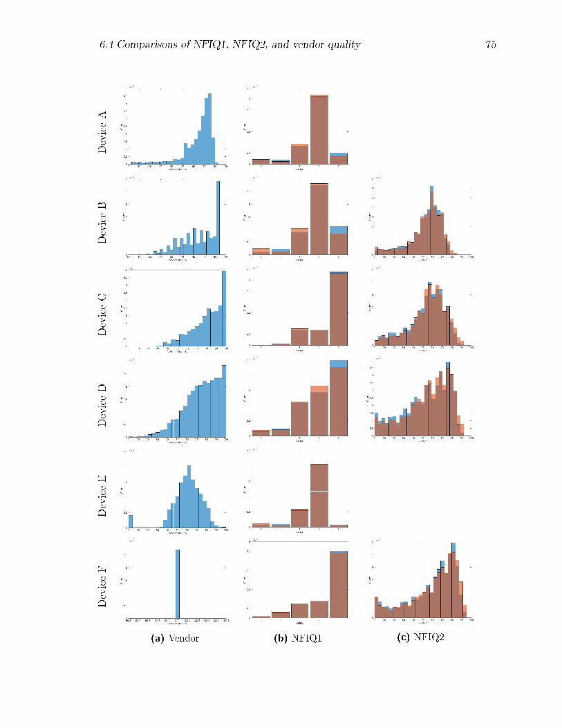
6.4 Comparisons of NFIQ1, NFIQ2, and vendor quality 75
DeviceA
DeviceB
DeviceC
DeviceD
DeviceE
DeviceF
(a) Vendor (b) NFIQ1 (c) NFIQ2
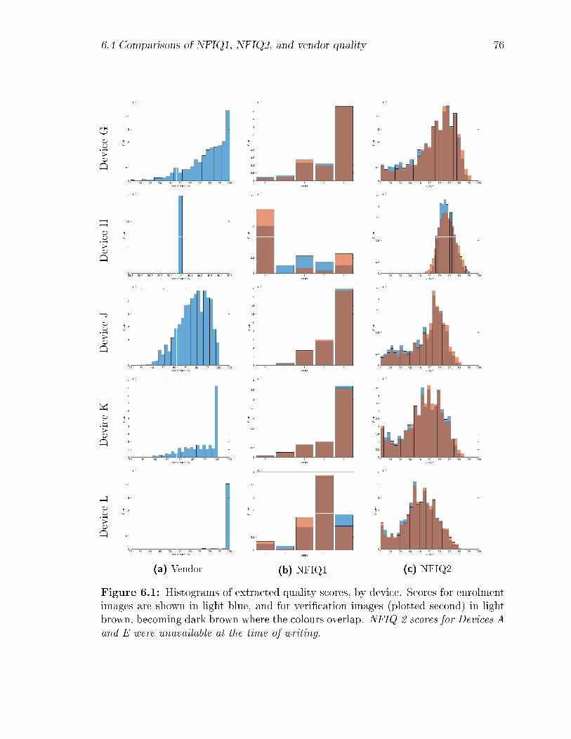
6.4 Comparisons of NFIQ1, NFIQ2, and vendor quality 76
DeviceG
DeviceH
DeviceJ
DeviceK
DeviceL
(a) Vendor (b) NFIQ1 (c) NFIQ2
Figure 6.1: Histograms of extracted quality scores, by device. Scores for enrolmentimages are shown in light blue, and for veri�cation images (plotted second) in lightbrown, becoming dark brown where the colours overlap. NFIQ-2 scores for Devices Aand E were unavailable at the time of writing.
6.5 E�ect of biometric quality on match score 77
6.5 E�ect of biometric quality on match score
Training of both NFIQ-1 and NFIQ-2 classi�ers is based on match score. Having
generated NFIQ scores and imported them into the Norwood database as described
in the preceding section, it becomes possible to label biometric match scores with
the NFIQ-1, NFIQ-2, and (where available) vendor-assessed quality values of their
constituent enrolment and veri�cation images, and explore the relationship between
quality and match score for the Norwood dataset. Since the demographics and capture
protocol of the ISBIT/Norwood study are likely quite di�erent from those used to
obtain the majority of the NFIQ training data, this is expected to be a useful test of
the broader applicability of the NFIQ measures.
In the case of enrolment, the ISBIT/Norwood protocol involves three presentations
of each of two �ngers, and hence associates six �ngerprint image records with each
enrolment template. While match scores are provided separately for each enrolled
�nger, it is not possible to break these down to a single enrolment image: indeed, the
enrolment protocol does not specify how the three single-�nger presentations are to be
used, so that vendors may (for example) have chosen a single preferred presentation,
or have aggregated presentations at either the image level or at the feature level.
Both NFIQ-1 and NFIQ-2 scores are returned, and stored in the Norwood database,
as integers1 but are cast to �oats for the purpose of averaging. In the case of NFIQ-1,
for which the quality score is a coarse ordinal scale from 1 (highest) to 5 (lowest), the
averaging provides somewhat �ner granularity.
Best, average, and worst enrolment image qualities are compared for NFIQ-1 in
Figure 6.2 and for NFIQ-2 in Figure 6.3. NFIQ-2 results are presented as simple
scatter plots, while for the NFIQ-1 results, the coarse score classes, especially for the
non-averaged cases, favour the use of box plots.
Although the protocol for veri�cation also involves multiple presentations, each
1As tinyint in the case of NFIQ-1, and as smallint in the case of NFIQ-2
6.5 E�ect of biometric quality on match score 78
results in a individual match score which we can identify uniquely with a single
veri�cation image. No averaging is employed in this case. Best, average, and worst
enrolment image qualities for NFIQ-1 and NFIQ-2 are compared in Figure 6.4.
Naïvely, one might expect (or at least hope) that genuine match score would be
simply correlated with the quality of either or both the enrolment and veri�cation
images. Perhaps unsurprisingly, the relationship is apparently not so straightforward.
Perhaps the most obvious way in which the NFIQ-1 box plots deviate from an
ideal quality-to-match score relationship is that they often display long tails of low
match score for the high quality classes. These tails are especially apparent in Devices
B, F, and J. Box plots for imposter match scores were omitted for clarity.
For NFIQ-2, the �gures (6.3 and 6.4) are in the form of scatter plots of match score
versus NFIQ-2 quality for both genuine and imposter scores. Genuine match scores
generally show a positive correlation with NFIQ-2 quality score, while (as might be
expected) imposter match scores are generally uncorrelated. However there is a rather
broad spread of match scores for the same assessed quality. In the case of Device F,
there is evidence of a subset whose NFIQ-2 quality score does not correlate at all
to match score. In devices K and L, we see some evidence of elevated (false) match
scores in the case of high quality imposters.
So far, results have been presented separately for enrolment quality and veri�ca-
tion quality. A natural question that arises is how the qualities combine in a single
match.
In order to probe this, genuine match scores were plotted against various composite
enrolment-veri�cation quality indices. Figure 6.5 shows two such indices: �rstly the
geometric mean of the (3-presentation average) enrolment and veri�cation NFIQ-2
scores; and secondly the reciprocal sum given by
21
NFIQ2enrol+ 1
NFIQ2verif
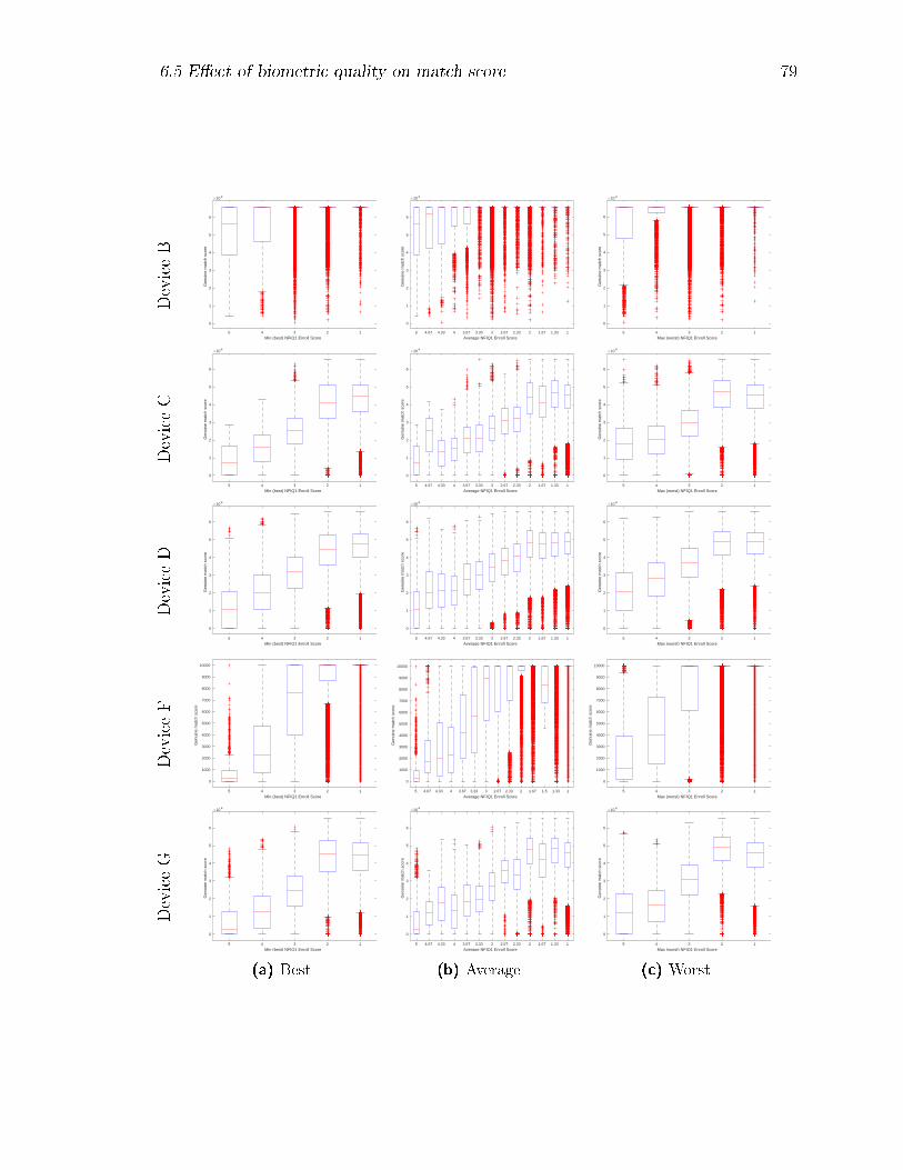
6.5 E�ect of biometric quality on match score 79
DeviceB
12345
Min (best) NFIQ1 Enroll Score
0
1
2
3
4
5
6
Gen
uine
mat
ch s
core
10 4
DeviceC
12345
Min (best) NFIQ1 Enroll Score
0
1
2
3
4
5
6
Gen
uine
mat
ch s
core
10 4
DeviceD
12345
Min (best) NFIQ1 Enroll Score
0
1
2
3
4
5
6
Gen
uine
mat
ch s
core
10 4
DeviceF
12345
Min (best) NFIQ1 Enroll Score
0
1000
2000
3000
4000
5000
6000
7000
8000
9000
10000
Gen
uine
mat
ch s
core
DeviceG
12345
Min (best) NFIQ1 Enroll Score
0
1
2
3
4
5
6
Gen
uine
mat
ch s
core
10 4
(a) Best
11.331.6722.332.6733.333.6744.334.675
Average NFIQ1 Enroll Score
0
1
2
3
4
5
6
Gen
uine
mat
ch s
core
10 4
11.331.6722.332.6733.333.6744.334.675
Average NFIQ1 Enroll Score
0
1
2
3
4
5
6
Gen
uine
mat
ch s
core
10 4
11.331.6722.332.6733.333.6744.334.675
Average NFIQ1 Enroll Score
0
1
2
3
4
5
6
Gen
uine
mat
ch s
core
10 4
11.331.51.6722.332.6733.333.6744.334.675
Average NFIQ1 Enroll Score
0
1000
2000
3000
4000
5000
6000
7000
8000
9000
10000
Gen
uine
mat
ch s
core
11.331.6722.332.6733.333.6744.334.675
Average NFIQ1 Enroll Score
0
1
2
3
4
5
6
Gen
uine
mat
ch s
core
10 4
(b) Average
12345
Max (worst) NFIQ1 Enroll Score
0
1
2
3
4
5
6
Gen
uine
mat
ch s
core
10 4
12345
Max (worst) NFIQ1 Enroll Score
0
1
2
3
4
5
6
Gen
uine
mat
ch s
core
10 4
12345
Max (worst) NFIQ1 Enroll Score
0
1
2
3
4
5
6
Gen
uine
mat
ch s
core
10 4
12345
Max (worst) NFIQ1 Enroll Score
0
1000
2000
3000
4000
5000
6000
7000
8000
9000
10000
Gen
uine
mat
ch s
core
12345
Max (worst) NFIQ1 Enroll Score
0
1
2
3
4
5
6
Gen
uine
mat
ch s
core
10 4
(c) Worst
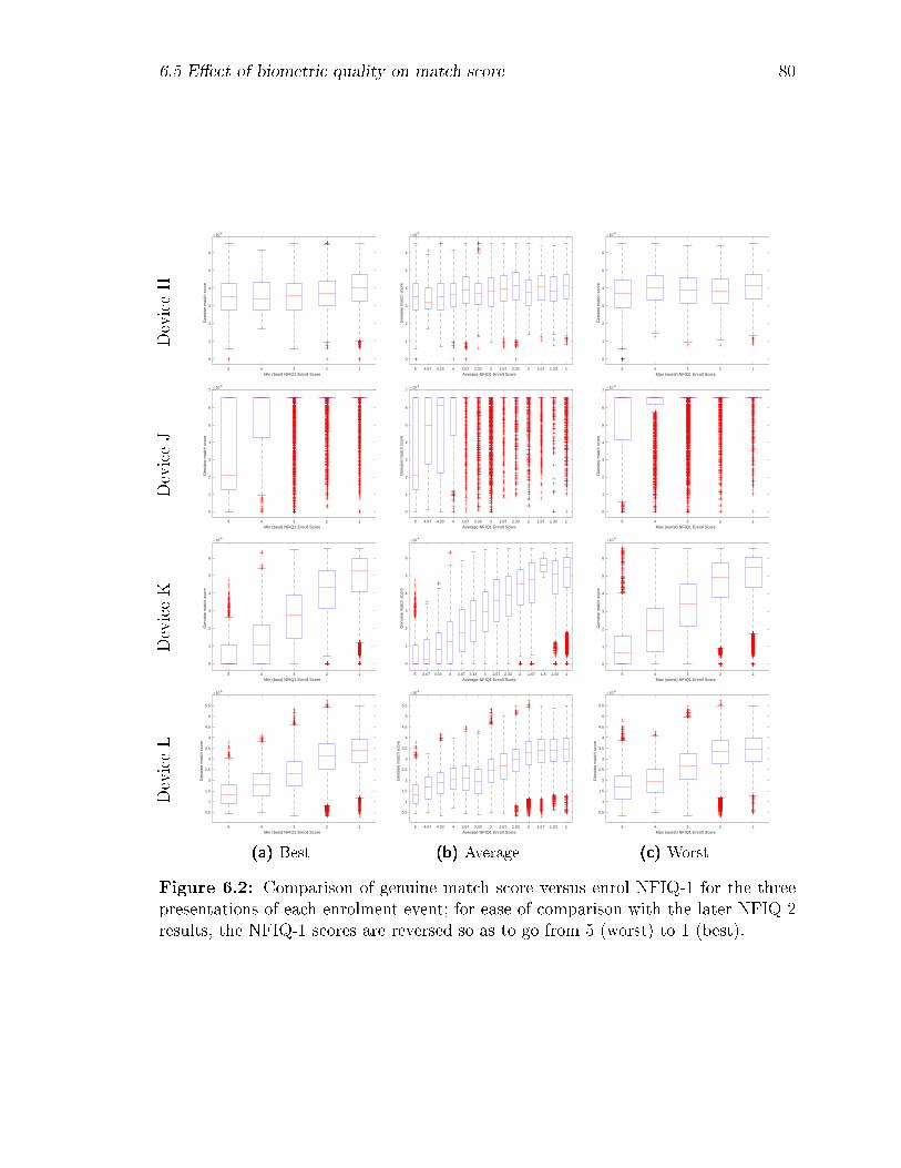
6.5 E�ect of biometric quality on match score 80
DeviceH
12345
Min (best) NFIQ1 Enroll Score
0
1
2
3
4
5
6
Gen
uine
mat
ch s
core
10 4
DeviceJ
12345
Min (best) NFIQ1 Enroll Score
0
1
2
3
4
5
6
7
Gen
uine
mat
ch s
core
10 4
DeviceK
12345
Min (best) NFIQ1 Enroll Score
0
1
2
3
4
5
6
Gen
uine
mat
ch s
core
10 4
DeviceL
12345
Min (best) NFIQ1 Enroll Score
0.5
1
1.5
2
2.5
3
3.5
4
4.5
5
5.5
Gen
uine
mat
ch s
core
10 4
(a) Best
11.331.6722.332.6733.333.6744.334.675
Average NFIQ1 Enroll Score
0
1
2
3
4
5
6
Gen
uine
mat
ch s
core
10 4
11.331.6722.332.6733.333.6744.334.675
Average NFIQ1 Enroll Score
0
1
2
3
4
5
6
7
Gen
uine
mat
ch s
core
10 4
11.331.51.6722.332.6733.333.6744.334.675
Average NFIQ1 Enroll Score
0
1
2
3
4
5
6
Gen
uine
mat
ch s
core
10 4
11.331.6722.332.6733.333.6744.334.675
Average NFIQ1 Enroll Score
0.5
1
1.5
2
2.5
3
3.5
4
4.5
5
5.5
Gen
uine
mat
ch s
core
10 4
(b) Average
12345
Max (worst) NFIQ1 Enroll Score
0
1
2
3
4
5
6
Gen
uine
mat
ch s
core
10 4
12345
Max (worst) NFIQ1 Enroll Score
0
1
2
3
4
5
6
7
Gen
uine
mat
ch s
core
10 4
12345
Max (worst) NFIQ1 Enroll Score
0
1
2
3
4
5
6
Gen
uine
mat
ch s
core
10 4
12345
Max (worst) NFIQ1 Enroll Score
0.5
1
1.5
2
2.5
3
3.5
4
4.5
5
5.5
Gen
uine
mat
ch s
core
10 4
(c) Worst
Figure 6.2: Comparison of genuine match score versus enrol NFIQ-1 for the threepresentations of each enrolment event; for ease of comparison with the later NFIQ-2results, the NFIQ-1 scores are reversed so as to go from 5 (worst) to 1 (best).
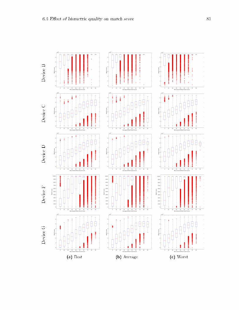
6.5 E�ect of biometric quality on match score 81
DeviceB
5 15 25 35 45 55 65 75 85 95
Max (best) NFIQ2 Enroll Score
0
1
2
3
4
5
6
Mat
ch s
core
10 4
DeviceC
5 15 25 35 45 55 65 75 85 95
Max (best) NFIQ2 Enroll Score
0
1
2
3
4
5
6
Mat
ch s
core
10 4
DeviceD
5 15 25 35 45 55 65 75 85 95
Max (best) NFIQ2 Enroll Score
0
1
2
3
4
5
6
Mat
ch s
core
10 4
DeviceF
5 15 25 35 45 55 65 75 85 95
Max (best) NFIQ2 Enroll Score
0
1000
2000
3000
4000
5000
6000
7000
8000
9000
10000
Mat
ch s
core
DeviceG
5 15 25 35 45 55 65 75 85 95
Max (best) NFIQ2 Enroll Score
0
1
2
3
4
5
6
Mat
ch s
core
10 4
(a) Best
5 15 25 35 45 55 65 75 85
Average NFIQ2 Enroll Score
0
1
2
3
4
5
6
Mat
ch s
core
10 4
5 15 25 35 45 55 65 75 85 95
Average NFIQ2 Enroll Score
0
1
2
3
4
5
6
Mat
ch s
core
10 4
5 15 25 35 45 55 65 75 85 95
Average NFIQ2 Enroll Score
0
1
2
3
4
5
6
Mat
ch s
core
10 4
5 15 25 35 45 55 65 75 85 95
Average NFIQ2 Enroll Score
0
1000
2000
3000
4000
5000
6000
7000
8000
9000
10000
Mat
ch s
core
5 15 25 35 45 55 65 75 85 95
Average NFIQ2 Enroll Score
0
1
2
3
4
5
6
Mat
ch s
core
10 4
(b) Average
5 15 25 35 45 55 65 75 85
Min (worst) NFIQ2 Enroll Score
0
1
2
3
4
5
6
Mat
ch s
core
10 4
5 15 25 35 45 55 65 75 85
Min (worst) NFIQ2 Enroll Score
0
1
2
3
4
5
6
Mat
ch s
core
10 4
5 15 25 35 45 55 65 75 85 95
Min (worst) NFIQ2 Enroll Score
0
1
2
3
4
5
6
Mat
ch s
core
10 4
5 15 25 35 45 55 65 75 85 95
Min (worst) NFIQ2 Enroll Score
0
1000
2000
3000
4000
5000
6000
7000
8000
9000
10000
Mat
ch s
core
5 15 25 35 45 55 65 75 85
Min (worst) NFIQ2 Enroll Score
0
1
2
3
4
5
6
Mat
ch s
core
10 4
(c) Worst
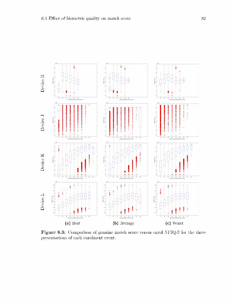
6.5 E�ect of biometric quality on match score 82
DeviceH
45 55 65 75 85 95
Max (best) NFIQ2 Enroll Score
0
1
2
3
4
5
6
Mat
ch s
core
10 4
DeviceJ
5 15 25 35 45 55 65 75 85
Max (best) NFIQ2 Enroll Score
0
1
2
3
4
5
6
Mat
ch s
core
10 4
DeviceK
5 15 25 35 45 55 65 75 85 95
Max (best) NFIQ2 Enroll Score
0
1
2
3
4
5
6
Mat
ch s
core
10 4
DeviceL
5 15 25 35 45 55 65 75 85
Max (best) NFIQ2 Enroll Score
0.5
1
1.5
2
2.5
3
3.5
4
4.5
5
5.5
Mat
ch s
core
10 4
(a) Best
45 55 65 75 85 95
Average NFIQ2 Enroll Score
0
1
2
3
4
5
6
Mat
ch s
core
10 4
5 15 25 35 45 55 65 75 85
Average NFIQ2 Enroll Score
0
1
2
3
4
5
6
7
Mat
ch s
core
10 4
5 15 25 35 45 55 65 75 85
Average NFIQ2 Enroll Score
0
1
2
3
4
5
6
Mat
ch s
core
10 4
5 15 25 35 45 55 65 75 85
Average NFIQ2 Enroll Score
0.5
1
1.5
2
2.5
3
3.5
4
4.5
5
5.5
Mat
ch s
core
10 4
(b) Average
35 45 55 65 75 85 95
Min (worst) NFIQ2 Enroll Score
0
1
2
3
4
5
6
Mat
ch s
core
10 4
5 15 25 35 45 55 65 75
Min (worst) NFIQ2 Enroll Score
0
1
2
3
4
5
6
Mat
ch s
core
10 4
5 15 25 35 45 55 65 75 85
Min (worst) NFIQ2 Enroll Score
0
1
2
3
4
5
6
Mat
ch s
core
10 4
5 15 25 35 45 55 65 75
Min (worst) NFIQ2 Enroll Score
0.5
1
1.5
2
2.5
3
3.5
4
4.5
5
5.5
Mat
ch s
core
10 4
(c) Worst
Figure 6.3: Comparison of genuine match score versus enrol NFIQ-2 for the threepresentations of each enrolment event.
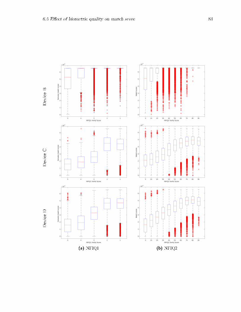
6.5 E�ect of biometric quality on match score 83
DeviceB
12345
NFIQ1 Verify Score
0
1
2
3
4
5
6
Gen
uine
mat
ch s
core
10 4
DeviceC
12345
NFIQ1 Verify Score
0
1
2
3
4
5
6
Gen
uine
mat
ch s
core
10 4
DeviceD
12345
NFIQ1 Verify Score
0
1
2
3
4
5
6
Gen
uine
mat
ch s
core
10 4
(a) NFIQ1
5 15 25 35 45 55 65 75 85 95
NFIQ2 Verify Score
0
1
2
3
4
5
6
Mat
ch s
core
10 4
5 15 25 35 45 55 65 75 85 95
NFIQ2 Verify Score
0
1
2
3
4
5
6
Mat
ch s
core
10 4
5 15 25 35 45 55 65 75 85 95
NFIQ2 Verify Score
0
1
2
3
4
5
6
Mat
ch s
core
10 4
(b) NFIQ2
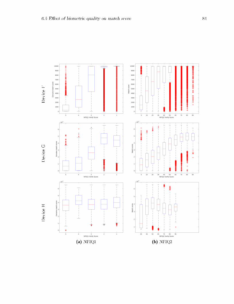
6.5 E�ect of biometric quality on match score 84
DeviceF
12345
NFIQ1 Verify Score
0
1000
2000
3000
4000
5000
6000
7000
8000
9000
10000
Gen
uine
mat
ch s
core
DeviceG
12345
NFIQ1 Verify Score
0
1
2
3
4
5
6
Gen
uine
mat
ch s
core
10 4
DeviceH
12345
NFIQ1 Verify Score
0
1
2
3
4
5
6
Gen
uine
mat
ch s
core
10 4
(a) NFIQ1
5 15 25 35 45 55 65 75 85 95
NFIQ2 Verify Score
0
1000
2000
3000
4000
5000
6000
7000
8000
9000
10000
Mat
ch s
core
5 15 25 35 45 55 65 75 85 95
NFIQ2 Verify Score
0
1
2
3
4
5
6
Mat
ch s
core
10 4
35 45 55 65 75 85 95
NFIQ2 Verify Score
1
2
3
4
5
6
Mat
ch s
core
10 4
(b) NFIQ2
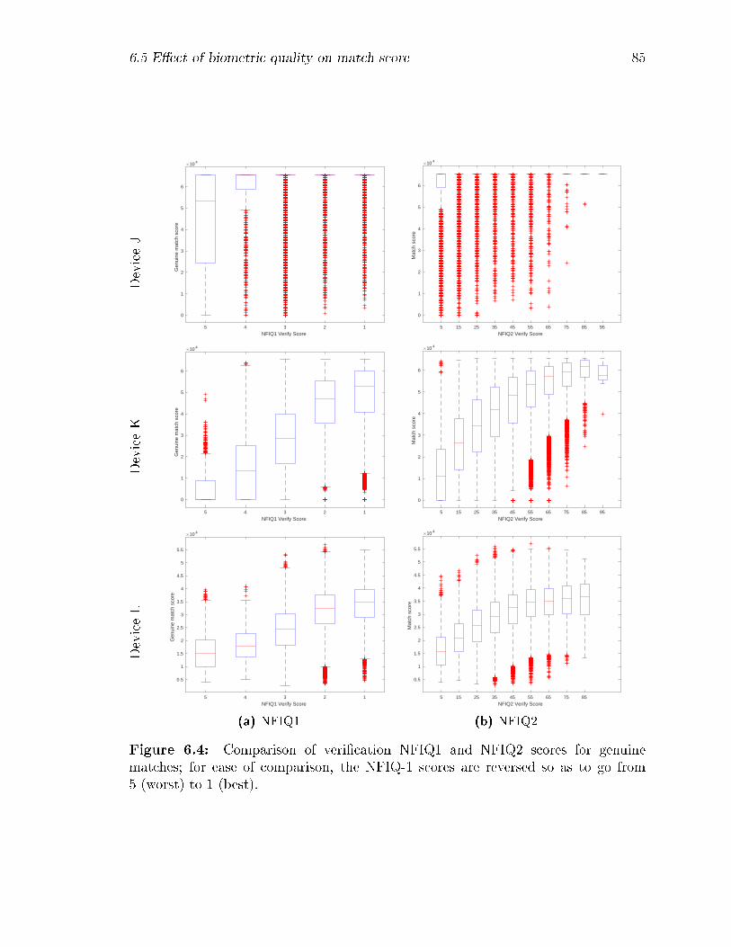
6.5 E�ect of biometric quality on match score 85
DeviceJ
12345
NFIQ1 Verify Score
0
1
2
3
4
5
6
Gen
uine
mat
ch s
core
10 4
DeviceK
12345
NFIQ1 Verify Score
0
1
2
3
4
5
6
Gen
uine
mat
ch s
core
10 4
DeviceL
12345
NFIQ1 Verify Score
0.5
1
1.5
2
2.5
3
3.5
4
4.5
5
5.5
Gen
uine
mat
ch s
core
10 4
(a) NFIQ1
5 15 25 35 45 55 65 75 85 95
NFIQ2 Verify Score
0
1
2
3
4
5
6
Mat
ch s
core
10 4
5 15 25 35 45 55 65 75 85 95
NFIQ2 Verify Score
0
1
2
3
4
5
6
Mat
ch s
core
10 4
5 15 25 35 45 55 65 75 85
NFIQ2 Verify Score
0.5
1
1.5
2
2.5
3
3.5
4
4.5
5
5.5
Mat
ch s
core
10 4
(b) NFIQ2
Figure 6.4: Comparison of veri�cation NFIQ1 and NFIQ2 scores for genuinematches; for ease of comparison, the NFIQ-1 scores are reversed so as to go from5 (worst) to 1 (best).
6.5 E�ect of biometric quality on match score 86
Compared with the individual results (Figures 6.3 and 6.4) it appears that com-
bining the qualities of both (average) enrolment and veri�cation results in a stronger
correlation with match score - in particular, it reduces the number of low quality �
high match score outliers.
In all these results, the behaviour of Device H is clearly anomalous: this is the
multispectral device whose NFIQ processing was troublesome and, as noted in the
previous section, should be treated as unreliable.
In the following sections we look more directly at classi�cation performance, by
means of Decision Error Trade-o� (DET) curves.

6.5 E�ect of biometric quality on match score 87
DeviceB
5 15 25 35 45 55 65 75 85
NFIQ2 Enrol-Verify Geom. Mean
0
1
2
3
4
5
6
Gen
uine
mat
ch s
core
10 4
DeviceC
5 15 25 35 45 55 65 75 85 95
NFIQ2 Enrol-Verify Geom. Mean
0
1
2
3
4
5
6
Gen
uine
mat
ch s
core
10 4
DeviceD
5 15 25 35 45 55 65 75 85 95
NFIQ2 Enrol-Verify Geom. Mean
0
1
2
3
4
5
6
Gen
uine
mat
ch s
core
10 4
(a) Geometric mean
5 15 25 35 45 55 65 75 85
NFIQ2 Enrol-Verify Recip.
0
1
2
3
4
5
6
Gen
uine
mat
ch s
core
10 4
5 15 25 35 45 55 65 75 85 95
NFIQ2 Enrol-Verify Recip.
0
1
2
3
4
5
6
Gen
uine
mat
ch s
core
10 4
5 15 25 35 45 55 65 75 85 95
NFIQ2 Enrol-Verify Recip.
0
1
2
3
4
5
6
Gen
uine
mat
ch s
core
10 4
(b) Reciprocal sum

6.5 E�ect of biometric quality on match score 88
DeviceF
5 15 25 35 45 55 65 75 85 95
NFIQ2 Enrol-Verify Geom. Mean
0
1000
2000
3000
4000
5000
6000
7000
8000
9000
10000
Gen
uine
mat
ch s
core
DeviceG
5 15 25 35 45 55 65 75 85 95
NFIQ2 Enrol-Verify Geom. Mean
0
1
2
3
4
5
6
Gen
uine
mat
ch s
core
10 4
DeviceH
45 55 65 75 85 95
NFIQ2 Enrol-Verify Geom. Mean
1
2
3
4
5
6
Gen
uine
mat
ch s
core
10 4
(a) Geometric mean
5 15 25 35 45 55 65 75 85 95
NFIQ2 Enrol-Verify Recip.
0
1000
2000
3000
4000
5000
6000
7000
8000
9000
10000
Gen
uine
mat
ch s
core
5 15 25 35 45 55 65 75 85 95
NFIQ2 Enrol-Verify Recip.
0
1
2
3
4
5
6
Gen
uine
mat
ch s
core
10 4
45 55 65 75 85 95
NFIQ2 Enrol-Verify Recip.
-2
-1
0
1
2
3
4
5
6
Gen
uine
mat
ch s
core
10 4
(b) Reciprocal sum
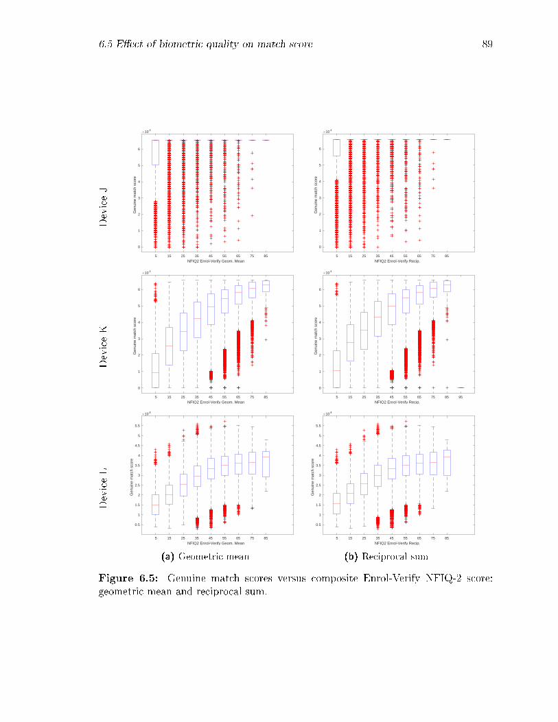
6.5 E�ect of biometric quality on match score 89
DeviceJ
5 15 25 35 45 55 65 75 85
NFIQ2 Enrol-Verify Geom. Mean
0
1
2
3
4
5
6
Gen
uine
mat
ch s
core
10 4
DeviceK
5 15 25 35 45 55 65 75 85
NFIQ2 Enrol-Verify Geom. Mean
0
1
2
3
4
5
6
Gen
uine
mat
ch s
core
10 4
DeviceL
5 15 25 35 45 55 65 75 85
NFIQ2 Enrol-Verify Geom. Mean
0.5
1
1.5
2
2.5
3
3.5
4
4.5
5
5.5
Gen
uine
mat
ch s
core
10 4
(a) Geometric mean
5 15 25 35 45 55 65 75 85
NFIQ2 Enrol-Verify Recip.
0
1
2
3
4
5
6
Gen
uine
mat
ch s
core
10 4
5 15 25 35 45 55 65 75 85 95
NFIQ2 Enrol-Verify Recip.
0
1
2
3
4
5
6
Gen
uine
mat
ch s
core
10 4
5 15 25 35 45 55 65 75 85
NFIQ2 Enrol-Verify Recip.
0.5
1
1.5
2
2.5
3
3.5
4
4.5
5
5.5
Gen
uine
mat
ch s
core
10 4
(b) Reciprocal sum
Figure 6.5: Genuine match scores versus composite Enrol-Verify NFIQ-2 score:geometric mean and reciprocal sum.
6.6 E�ect of biometric quality on classi�cation accuracy 90
6.6 E�ect of biometric quality on classi�cation accuracy
The previous section examined the relationship between biometric quality and match
score for individual match pairs. Here, we consider its impact on overall classi�cation
accuracy of a biometric IDMS.
The classi�cation accuracy was explored using Decision Error Trade-o� (DET)
curves, broken down as before by device. The procedure for evaluating classi�cation
performance versus quality was based on selecting subsets of the available data based
on their quality indices, and constructing DET curves for each subset. Based on the
preceding results, the arithmetic mean of the three enrolment image qualities was
used in all cases.
In the quality screening application, the idea would be to reject some low quality
presentations: during enrolment (perhaps forcing enrolment of a di�erent - higher
quality - �nger) and/or during veri�cation (for example, declining to attempt a match
of a poorly presented or occluded �nger). In order not to diminish signi�cantly the
overall convenience of the system, it would be desirable to limit to a small fraction
the number of such rejected presentations. Thus we seek a quality threshold that
is e�ective at improving overall classi�cation accuracy, while limiting the increase in
failure to enrol (FTE).
When comparing quality metrics in this application, we should ideally do so at
the same fraction of rejected presentations i.e. compare the increase in classi�cation
performance for the same decrease in convenience. Since NFIQ-1 classi�es images
into one of �ve discrete quality classes, it provides little scope for precise control of
the rejected fraction: at best, we can really only reject all of the lowest quality class
- with the caveat that this may correspond to a quite widely varying fraction of cases
from device to device. For example, referring to the histograms of Figure 6.1, we see
that Devices C and J classify less than 1 % of images at the lowest NFIQ-1 quality
(Class 5) whereas Devices B and L have up to 6 % in this class. (Device H apparently

6.6 E�ect of biometric quality on classi�cation accuracy 91
Table 6.1: Excluded percentages x of the lowest quality NFIQ-1 class (Class 5) andthe corresponding thresholds (lower xth percentiles) for exclusion from NFIQ-2
Device IDNFIQ-1 NFIQ-2
Enrol % Verify % Enrol Thresh. Verify Thresh.B. 1.7 4.8 6.0 13.0C. 0.2 0.3 2.0 2.0D. 2.9 3.4 4.0 6.0F. 1.5 1.9 1.3 2.0G. 3.1 2.8 7.0 6.0H. 51.0 69.1 67.3 72.0J. 0.2 0.2 1.3 0.0K. 1.4 1.7 1.7 1.0L. 4.6 6.1 5.0 7.0
shows anomalously high (50-70 %) in NFIQ-1 Class 5, but we believe those results to
be erroneous, and due to the particular biometric capture technology of the device.)
In contrast, NFIQ-2 has a much more expressive quality scale, from 1-100, which
allows quite precise rejection below (or above) a given quality percentile.
In order to compare the e�cacy of NFIQ-2 versus NFIQ-1 for this application, we
therefore �rst evaluated the change in overall classi�cation performance obtained by
eliminating the lowest NFIQ-1 quality class (from both enrolment and veri�cation),
noting for each device the percentage of enrolments and veri�cations removed. Then
we repeated the evaluation, thresholding the NFIQ-2 scores at the same percentiles
(Figure 6.6). Table 6.1 summarizes the percentiles and thresholds.
Although of little practical value, it is also scienti�cally interesting to consider the
e�ect of excluding the highest quality matches. Table 6.2 shows the corresponding
percentages of NFIQ-1 Class 1 enrolments and veri�cations, and NFIQ-2 thresholds
by device for this case. Figure 6.7 presents results for each device side-by-side, with
the baseline DET curve in black, the results with lowest quality matches removed in
green, and those with highest quality scores removed in red.
Taken device by device, we see that there is very little to distinguish the perfor-
mance of NFIQ-2 versus NFIQ-1 at the same percentage of rejected presentations. If

6.6 E�ect of biometric quality on classi�cation accuracy 92
𝜃𝐿 𝜃𝐻
Percentage
NFIQ-1 score distribution
NFIQ-2 score distribution
Remove lowest quality
Remove highest quality
Figure 6.6: Schematic representation of the conversion of NFIQ-1 class percentagesinto NFIQ-2 thresholds. The correspondence is applied separately for enrolment andveri�cation quality scores.
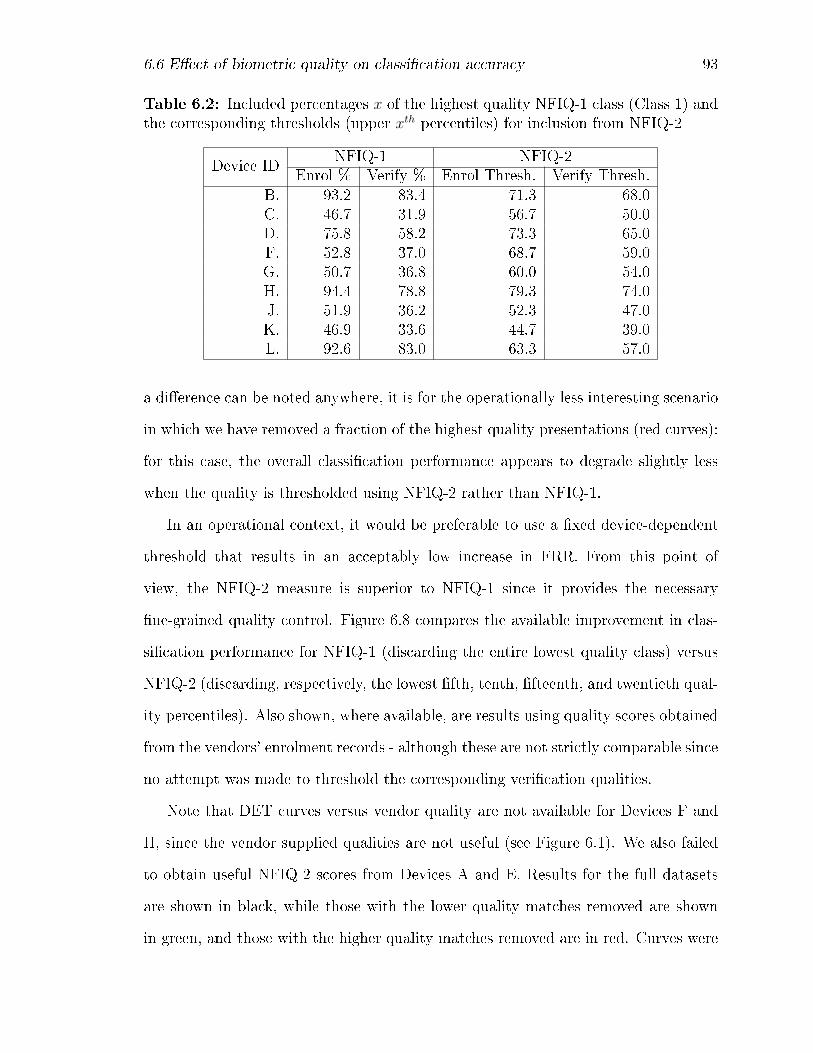
6.6 E�ect of biometric quality on classi�cation accuracy 93
Table 6.2: Included percentages x of the highest quality NFIQ-1 class (Class 1) andthe corresponding thresholds (upper xth percentiles) for inclusion from NFIQ-2
Device IDNFIQ-1 NFIQ-2
Enrol % Verify % Enrol Thresh. Verify Thresh.B. 93.2 83.4 71.3 68.0C. 46.7 31.9 56.7 50.0D. 75.8 58.2 73.3 65.0F. 52.8 37.0 68.7 59.0G. 50.7 36.8 60.0 54.0H. 94.4 78.8 79.3 74.0J. 51.9 36.2 52.3 47.0K. 46.9 33.6 44.7 39.0L. 92.6 83.0 63.3 57.0
a di�erence can be noted anywhere, it is for the operationally less interesting scenario
in which we have removed a fraction of the highest quality presentations (red curves):
for this case, the overall classi�cation performance appears to degrade slightly less
when the quality is thresholded using NFIQ-2 rather than NFIQ-1.
In an operational context, it would be preferable to use a �xed device-dependent
threshold that results in an acceptably low increase in FRR. From this point of
view, the NFIQ-2 measure is superior to NFIQ-1 since it provides the necessary
�ne-grained quality control. Figure 6.8 compares the available improvement in clas-
si�cation performance for NFIQ-1 (discarding the entire lowest quality class) versus
NFIQ-2 (discarding, respectively, the lowest �fth, tenth, �fteenth, and twentieth qual-
ity percentiles). Also shown, where available, are results using quality scores obtained
from the vendors' enrolment records - although these are not strictly comparable since
no attempt was made to threshold the corresponding veri�cation qualities.
Note that DET curves versus vendor quality are not available for Devices F and
H, since the vendor supplied qualities are not useful (see Figure 6.1). We also failed
to obtain useful NFIQ-2 scores from Devices A and E. Results for the full datasets
are shown in black, while those with the lower quality matches removed are shown
in green, and those with the higher quality matches removed are in red. Curves were
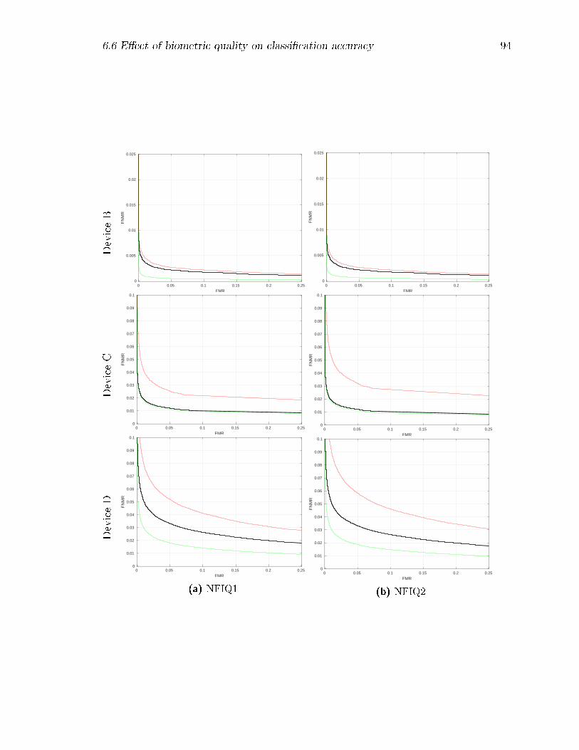
6.6 E�ect of biometric quality on classi�cation accuracy 94
DeviceB
0 0.05 0.1 0.15 0.2 0.25
FMR
0
0.005
0.01
0.015
0.02
0.025
FN
MR
DeviceC
0 0.05 0.1 0.15 0.2 0.25
FMR
0
0.01
0.02
0.03
0.04
0.05
0.06
0.07
0.08
0.09
0.1
FN
MR
DeviceD
0 0.05 0.1 0.15 0.2 0.25
FMR
0
0.01
0.02
0.03
0.04
0.05
0.06
0.07
0.08
0.09
0.1
FN
MR
(a) NFIQ1
0 0.05 0.1 0.15 0.2 0.25
FMR
0
0.005
0.01
0.015
0.02
0.025
FN
MR
0 0.05 0.1 0.15 0.2 0.25
FMR
0
0.01
0.02
0.03
0.04
0.05
0.06
0.07
0.08
0.09
0.1
FN
MR
0 0.05 0.1 0.15 0.2 0.25
FMR
0
0.01
0.02
0.03
0.04
0.05
0.06
0.07
0.08
0.09
0.1
FN
MR
(b) NFIQ2
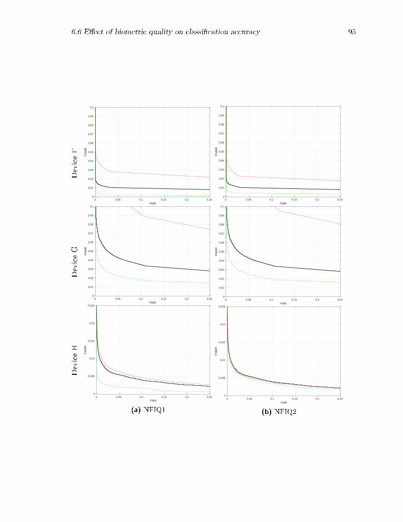
6.6 E�ect of biometric quality on classi�cation accuracy 95
DeviceF
0 0.05 0.1 0.15 0.2 0.25
FMR
0
0.01
0.02
0.03
0.04
0.05
0.06
0.07
0.08
0.09
0.1
FN
MR
DeviceG
0 0.05 0.1 0.15 0.2 0.25
FMR
0
0.01
0.02
0.03
0.04
0.05
0.06
0.07
0.08
0.09
0.1
FN
MR
DeviceH
0 0.05 0.1 0.15 0.2 0.25
FMR
0
0.005
0.01
0.015
0.02
0.025
FN
MR
(a) NFIQ1
0 0.05 0.1 0.15 0.2 0.25
FMR
0
0.01
0.02
0.03
0.04
0.05
0.06
0.07
0.08
0.09
0.1
FN
MR
0 0.05 0.1 0.15 0.2 0.25
FMR
0
0.01
0.02
0.03
0.04
0.05
0.06
0.07
0.08
0.09
0.1
FN
MR
0 0.05 0.1 0.15 0.2 0.25
FMR
0
0.005
0.01
0.015
0.02
0.025
FN
MR
(b) NFIQ2

6.6 E�ect of biometric quality on classi�cation accuracy 96
DeviceJ
0 0.05 0.1 0.15 0.2 0.25
FMR
0
1
2
3
4
5
6
7
8
9
10
FN
MR
10 -3
DeviceK
0 0.05 0.1 0.15 0.2 0.25
FMR
0
0.05
0.1
0.15
0.2
0.25
FN
MR
DeviceL
0 0.05 0.1 0.15 0.2 0.25
FMR
0
0.01
0.02
0.03
0.04
0.05
0.06
0.07
0.08
0.09
0.1
FN
MR
(a) NFIQ1
0 0.05 0.1 0.15 0.2 0.25
FMR
0
1
2
3
4
5
6
7
8
9
10
FN
MR
10 -3
0 0.05 0.1 0.15 0.2 0.25
FMR
0
0.05
0.1
0.15
0.2
0.25
FN
MR
0 0.05 0.1 0.15 0.2 0.25
FMR
0
0.01
0.02
0.03
0.04
0.05
0.06
0.07
0.08
0.09
0.1
FN
MR
(b) NFIQ2
Figure 6.7: Comparison of classi�cation performance by device versus quality forthe NFIQ measures. For NFIQ-1, the DET is evaluated for NFIQ with all results(black), with lowest quality class removed (green) and with the highest quality classremoved (red), noting in each case the percentage of cases removed. CorrespondingNFIQ-2 results are obtained by thresholding the data at the same percentages asthose recorded for NFIQ-1.
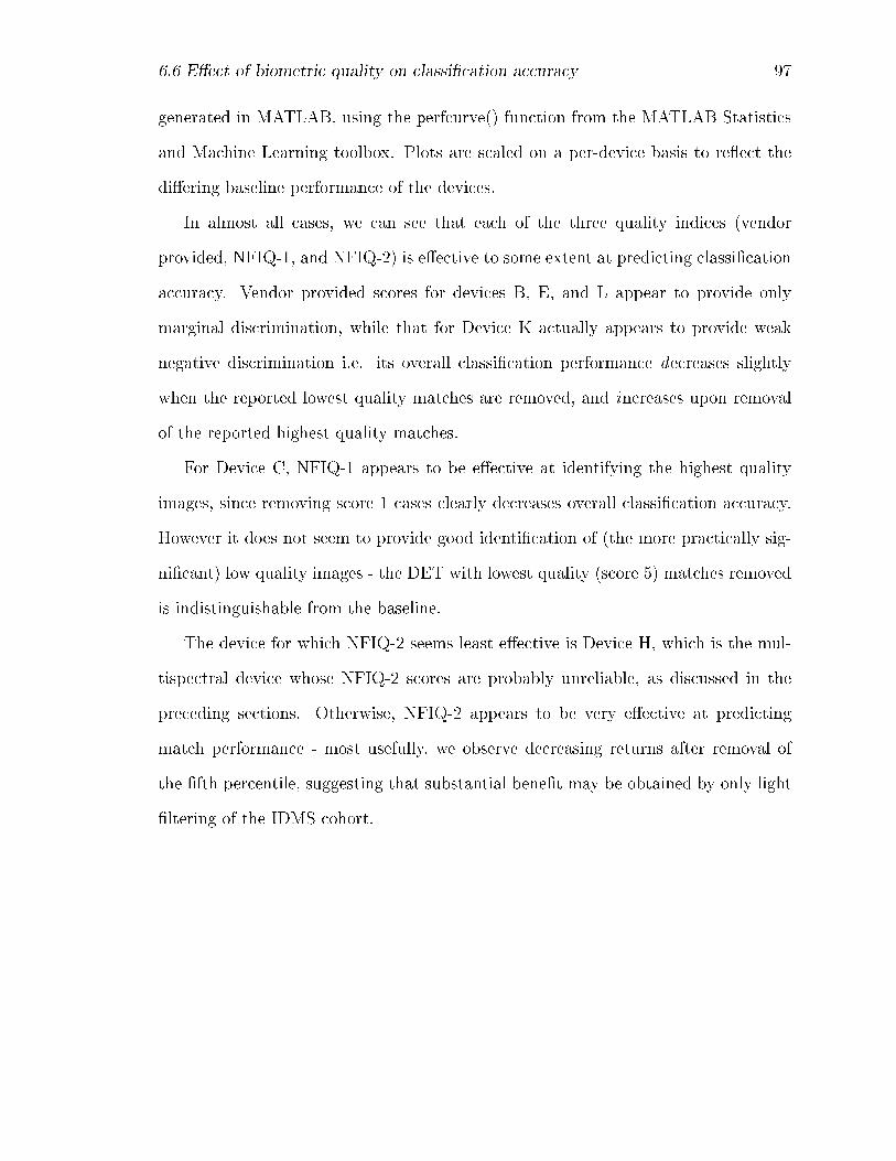
6.6 E�ect of biometric quality on classi�cation accuracy 97
generated in MATLAB, using the perfcurve() function from the MATLAB Statistics
and Machine Learning toolbox. Plots are scaled on a per-device basis to re�ect the
di�ering baseline performance of the devices.
In almost all cases, we can see that each of the three quality indices (vendor
provided, NFIQ-1, and NFIQ-2) is e�ective to some extent at predicting classi�cation
accuracy. Vendor provided scores for devices B, E, and L appear to provide only
marginal discrimination, while that for Device K actually appears to provide weak
negative discrimination i.e. its overall classi�cation performance decreases slightly
when the reported lowest quality matches are removed, and increases upon removal
of the reported highest quality matches.
For Device C, NFIQ-1 appears to be e�ective at identifying the highest quality
images, since removing score 1 cases clearly decreases overall classi�cation accuracy.
However it does not seem to provide good identi�cation of (the more practically sig-
ni�cant) low quality images - the DET with lowest quality (score 5) matches removed
is indistinguishable from the baseline.
The device for which NFIQ-2 seems least e�ective is Device H, which is the mul-
tispectral device whose NFIQ-2 scores are probably unreliable, as discussed in the
preceding sections. Otherwise, NFIQ-2 appears to be very e�ective at predicting
match performance - most usefully, we observe decreasing returns after removal of
the �fth percentile, suggesting that substantial bene�t may be obtained by only light
�ltering of the IDMS cohort.
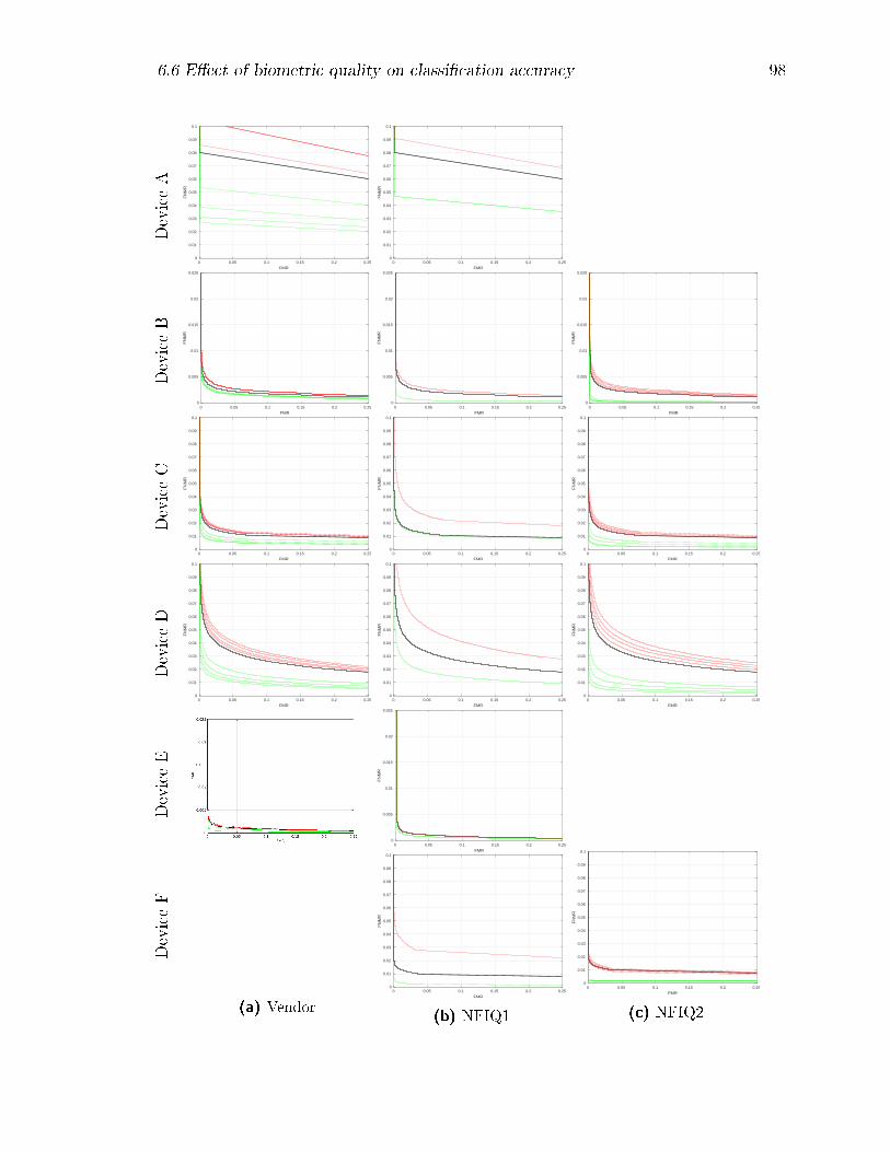
6.6 E�ect of biometric quality on classi�cation accuracy 98
DeviceA
0 0.05 0.1 0.15 0.2 0.25
FMR
0
0.01
0.02
0.03
0.04
0.05
0.06
0.07
0.08
0.09
0.1
FN
MR
DeviceB
0 0.05 0.1 0.15 0.2 0.25
FMR
0
0.005
0.01
0.015
0.02
0.025
FN
MR
DeviceC
0 0.05 0.1 0.15 0.2 0.25
FMR
0
0.01
0.02
0.03
0.04
0.05
0.06
0.07
0.08
0.09
0.1
FN
MR
DeviceD
0 0.05 0.1 0.15 0.2 0.25
FMR
0
0.01
0.02
0.03
0.04
0.05
0.06
0.07
0.08
0.09
0.1
FN
MR
DeviceE
DeviceF
(a) Vendor
0 0.05 0.1 0.15 0.2 0.25
FMR
0
0.01
0.02
0.03
0.04
0.05
0.06
0.07
0.08
0.09
0.1
FN
MR
0 0.05 0.1 0.15 0.2 0.25
FMR
0
0.005
0.01
0.015
0.02
0.025
FN
MR
0 0.05 0.1 0.15 0.2 0.25
FMR
0
0.01
0.02
0.03
0.04
0.05
0.06
0.07
0.08
0.09
0.1
FN
MR
0 0.05 0.1 0.15 0.2 0.25
FMR
0
0.01
0.02
0.03
0.04
0.05
0.06
0.07
0.08
0.09
0.1
FN
MR
0 0.05 0.1 0.15 0.2 0.25
FMR
0
0.005
0.01
0.015
0.02
0.025
FN
MR
0 0.05 0.1 0.15 0.2 0.25
FMR
0
0.01
0.02
0.03
0.04
0.05
0.06
0.07
0.08
0.09
0.1
FN
MR
(b) NFIQ1
0 0.05 0.1 0.15 0.2 0.25
FMR
0
0.005
0.01
0.015
0.02
0.025
FN
MR
0 0.05 0.1 0.15 0.2 0.25
FMR
0
0.01
0.02
0.03
0.04
0.05
0.06
0.07
0.08
0.09
0.1
FN
MR
0 0.05 0.1 0.15 0.2 0.25
FMR
0
0.01
0.02
0.03
0.04
0.05
0.06
0.07
0.08
0.09
0.1
FN
MR
0 0.05 0.1 0.15 0.2 0.25
FMR
0
0.01
0.02
0.03
0.04
0.05
0.06
0.07
0.08
0.09
0.1
FN
MR
(c) NFIQ2
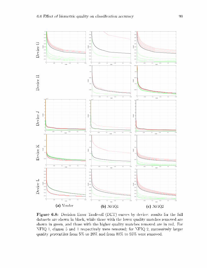
6.6 E�ect of biometric quality on classi�cation accuracy 99
DeviceG
0 0.05 0.1 0.15 0.2 0.25
FMR
0
0.01
0.02
0.03
0.04
0.05
0.06
0.07
0.08
0.09
0.1
FN
MR
DeviceH
DeviceJ
0 0.05 0.1 0.15 0.2 0.25
FMR
0
1
2
3
4
5
6
7
8
9
10
FN
MR
10 -3
DeviceK
0 0.05 0.1 0.15 0.2 0.25
FMR
0
0.05
0.1
0.15
0.2
0.25
FN
MR
DeviceL
0 0.05 0.1 0.15 0.2 0.25
FMR
0
0.01
0.02
0.03
0.04
0.05
0.06
0.07
0.08
0.09
0.1
FN
MR
(a) Vendor
0 0.05 0.1 0.15 0.2 0.25
FMR
0
0.01
0.02
0.03
0.04
0.05
0.06
0.07
0.08
0.09
0.1
FN
MR
0 0.05 0.1 0.15 0.2 0.25
FMR
0
0.005
0.01
0.015
0.02
0.025
FN
MR
0 0.05 0.1 0.15 0.2 0.25
FMR
0
1
2
3
4
5
6
7
8
9
10
FN
MR
10 -3
0 0.05 0.1 0.15 0.2 0.25
FMR
0
0.05
0.1
0.15
0.2
0.25
FN
MR
0 0.05 0.1 0.15 0.2 0.25
FMR
0
0.01
0.02
0.03
0.04
0.05
0.06
0.07
0.08
0.09
0.1
FN
MR
(b) NFIQ1
0 0.05 0.1 0.15 0.2 0.25
FMR
0
0.01
0.02
0.03
0.04
0.05
0.06
0.07
0.08
0.09
0.1
FN
MR
0 0.05 0.1 0.15 0.2 0.25
FMR
0
0.005
0.01
0.015
0.02
0.025
FN
MR
0 0.05 0.1 0.15 0.2 0.25
FMR
0
1
2
3
4
5
6
7
8
9
10
FN
MR
10 -3
0 0.05 0.1 0.15 0.2 0.25
FMR
0
0.05
0.1
0.15
0.2
0.25
FN
MR
0 0.05 0.1 0.15 0.2 0.25
FMR
0
0.01
0.02
0.03
0.04
0.05
0.06
0.07
0.08
0.09
0.1
FN
MR
(c) NFIQ2
Figure 6.8: Decision Error Trade-o� (DET) curves by device: results for the fulldatasets are shown in black, while those with the lower quality matches removed areshown in green, and those with the higher quality matches removed are in red. ForNFIQ-1, classes 5 and 1 respectively were removed; for NFIQ-2, successively largerquality percentiles from 5% to 20% and from 80% to 95% were removed.
6.7 Discussion 100
6.7 Discussion
The goal of the chapter was to understand the relationship between NFIQ-1 and
NFIQ-1 scores (and, where available, vendor-speci�c quality scores obtained during
template enrolment), and the relationship between these scores and the measured
biometric performance - both in terms of raw match scores and overall classi�cation
accuracy.
We have seen that both NFIQ-1 and NFIQ-2 are e�ective predictive tools for
genuine match score, across a broad range of �ngerprint capture devices with di�erent
(vendor-dependent) image and match score processing.
We have shown how both may be used to validate or sanitize �ngerprint presen-
tations by rejecting a fraction of the lowest indicated quality, in order to improve the
overall classi�cation performance of a biometric IDMS with minimal degradation in
convenience (FTE). When compared at the same fraction of rejected presentations
(i.e. the same increase in FTE), NFIQ-1 and NFIQ-2 perform similarly in terms of
the potential decrease in FNMR at a given FMR. However, the more expressive 1-
100 quality scale of NFIQ-2 gives it the signi�cant advantage of allowing the system
integrator to choose a more precise quality threshold for exclusion.
Chapter 7
Identi�cation and demographics of a
biometric menagerie, and its e�ect on
classi�cation performance and
template ageing
In the previous chapter, it was shown that both NFIQ-1 and NFIQ-2 measures are
e�ective at identifying low quality �ngerprints, and how selective rejection of such
�ngerprints can improve the overall classi�cation performance of a �ngerprint-based
IDMS.
The goals of this chapter are twofold: �rst, to explore the demographics of �nger-
print quality, in particular to see if we can identify any common demographic traits
among the subjects whose �ngerprints are identi�ed by NFIQ as low quality. We
attempt to put these individuals in the context of Doddington's biometric �zoo� [17].
Secondly, we re-visit the topic of template ageing (Chapter 5), and examine whether a
relatively small cohort of low �ngerprint quality individuals disproportionately a�ects
template ageing behaviour.
101
7.1 Revisiting Doddington's zoo 102
The demographics of NFIQ-1/NFIQ-2 quality for the ISBIT/Norwood data set as
a whole was reported recently by Rong (Roy) Yang in �E�ects of sensors, age, and
gender on �ngerprint image quality� [85], Chapter 5 �Results and Discussions� and
will not be revisited here. Brie�y, it was found that both NFIQ-1 and NFIQ-2 quality
scores were generally higher for males than for females, and for younger than for older
subjects � with the exception of the multi-spectral Device H for which the opposite
behaviour was observed.
7.1 Revisiting Doddington's zoo
7.1.1 Identi�cation of a common Goat subset
Doddington's original classi�cation of biometric �goats� was based on sorting in in-
creasing order of genuine match score, and taking the lowest 2.5th percentile of indi-
viduals [17]. In our scenario, we must deal with match scores from multiple devices,
whose vendor-speci�c scoring algorithms do not permit an overall ordering. Instead,
we developed the following classi�cation scheme.
First, choose a common target FNMR across all devices: preferably this should
be small enough to be operationally reasonable, yet large enough that it gives a
measurable count of false non-matches on every device1. More precisely, we would
like to have enough false non-matches to make a low-variance estimate of the FNMR.
Then, for each device, determine the decision threshold corresponding to the target
FNMR, and evaluate a confusion matrix at that threshold for each subject-�nger,
taken over all the available visit pairs. Note that there is some multiplicity here
since the protocol for a verify visit consists of two veri�cation attempts of three
presentations each: this helps to �ll out the confusion matrices in spite of the relatively
1The number of genuine matches per visit pair is relatively small due to the limited number ofsubjects, and not all devices were present in every visit
7.1 Revisiting Doddington's zoo 103
small number of visit pairs.
At this point, Device J was eliminated because it was not possible to determine
a suitable threshold for the target 5 % FNMR, and Device A because, although a
putative threshold was determined, the actual FNMR at that threshold di�ered sig-
ni�cantly from the target FNMR, for reasons as yet undetermined.
The true match (TM), false non-match (FNM), false match (FM) and true non-
match (TNM) counts for the remaining devices were then aggregated, and the subject-
�ngers sorted in order by number of false non-matches (FNM), from highest to lowest.
We then de�ned as the �goat set� the set of subject �ngers that together accounted
for 50 % of the total false non-matches. Note that although FNMR values in excess
of 55 % are observed for individual subject-�ngers, the overall FNMR for each device,
as well as for the aggregate subject-�nger set as a whole, is constrained to the target
5 % (aggregate TM = 722895, FNM = 38081).
The choice of 50 % is somewhat arbitrary, however it results in a conveniently-
sized subset of 29 out of the 879 available unique subject-�ngers (Table 7.1). For a
key to the numerical �nger position identi�ers used, see Table 7.2.
A question that arises naturally is whether the �Goat set� established by this
procedure re�ects an aggregation of substantially disjoint sets of high FNMR matches
from each separate device, or whether it indicates a set of subject-�ngers that is
intrinsically susceptible to false non-matches regardless of device, and whose members
in some sense therefore provide less information about the identity of the subject.
To explore this question, the confusion matrices of the individual devices were
ordered by FNM in the same manner as for the aggregate set, and their own goat
sets constructed as the subject-�ngers that accounted for 50 % of the total false non-
matches of the device. A search was then made for each of the aggregate Goat
subject-�ngers in each of the individual devices' Goat sets.
Figure 7.1 shows the counts of how many devices each Goat appears in, clearly
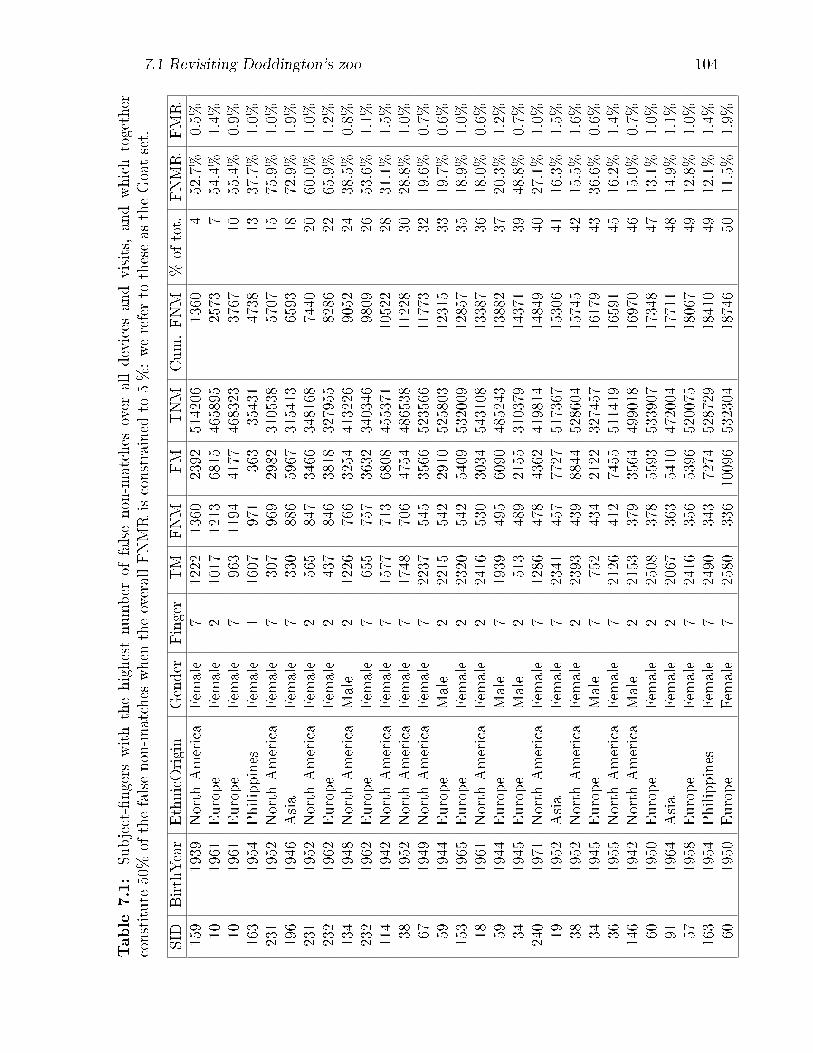
7.1 Revisiting Doddington's zoo 104
Table
7.1:
Subject-�ngers
withthehighestnumber
offalsenon-m
atches
over
alldevices
andvisits,
andwhichtogether
constitute
50%
ofthefalsenon-m
atches
when
theoverallFNMRisconstrained
to5%:wereferto
theseas
theGoatset.
SID
BirthYear
EthnicOrigin
Gender
Finger
TM
FNM
FM
TNM
Cum.FNM
%of
tot.
FNMR
FMR
159
1939
North
America
Fem
ale
71222
1360
2392
514206
1360
452.7%
0.5%
101961
Europe
Fem
ale
21017
1213
6815
465895
2573
754.4%
1.4%
101961
Europe
Fem
ale
7963
1194
4177
468323
3767
1055.4%
0.9%
163
1954
Philippines
Fem
ale
11607
971
363
35431
4738
1337.7%
1.0%
231
1952
North
America
Fem
ale
7307
969
2982
310538
5707
1575.9%
1.0%
196
1946
Asia
Fem
ale
7330
886
5967
315413
6593
1872.9%
1.9%
231
1952
North
America
Fem
ale
2565
847
3466
348168
7440
2060.0%
1.0%
232
1962
Europe
Fem
ale
2437
846
3818
327955
8286
2265.9%
1.2%
134
1948
North
America
Male
21226
766
3254
413226
9052
2438.5%
0.8%
232
1962
Europe
Fem
ale
7655
757
3632
340346
9809
2653.6%
1.1%
114
1942
North
America
Fem
ale
71577
713
6808
455371
10522
2831.1%
1.5%
381952
North
America
Fem
ale
71748
706
4754
486538
11228
3028.8%
1.0%
671949
North
America
Fem
ale
72237
545
3566
523566
11773
3219.6%
0.7%
591944
Europe
Male
22215
542
2910
525803
12315
3319.7%
0.6%
153
1965
Europe
Fem
ale
22320
542
5409
532009
12857
3518.9%
1.0%
181961
North
America
Fem
ale
22416
530
3034
543108
13387
3618.0%
0.6%
591944
Europe
Male
71939
495
6090
485243
13882
3720.3%
1.2%
341945
Europe
Male
2513
489
2155
310379
14371
3948.8%
0.7%
240
1971
North
America
Fem
ale
71286
478
4362
419814
14849
4027.1%
1.0%
191952
Asia
Fem
ale
72341
457
7727
517367
15306
4116.3%
1.5%
381952
North
America
Fem
ale
22393
439
8844
528604
15745
4215.5%
1.6%
341945
Europe
Male
7752
434
2122
327457
16179
4336.6%
0.6%
361955
North
America
Fem
ale
72126
412
7455
511419
16591
4516.2%
1.4%
146
1942
North
America
Male
22153
379
3564
499018
16970
4615.0%
0.7%
601950
Europe
Fem
ale
22508
378
5593
533907
17348
4713.1%
1.0%
911964
Asia
Fem
ale
22067
363
5410
472004
17711
4814.9%
1.1%
571958
Europe
Fem
ale
72416
356
5396
520075
18067
4912.8%
1.0%
163
1954
Philippines
Fem
ale
72490
343
7274
528729
18410
4912.1%
1.4%
601950
Europe
Fem
ale
72580
336
10096
532304
18746
5011.5%
1.9%
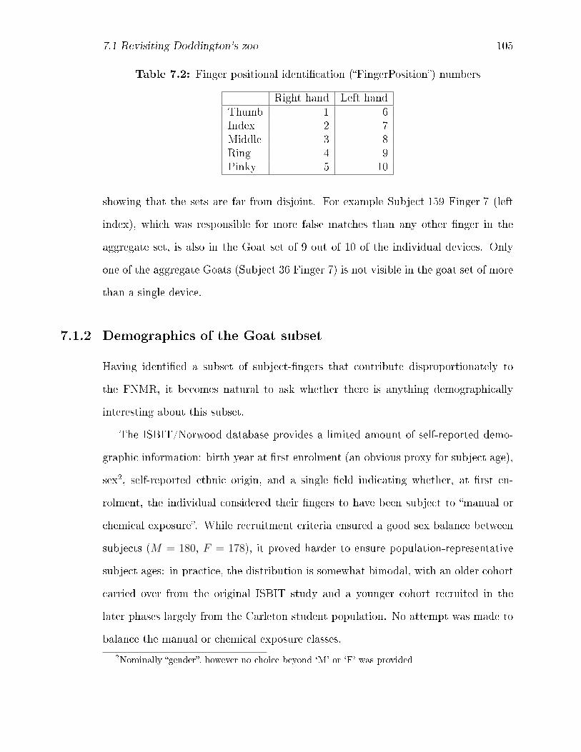
7.1 Revisiting Doddington's zoo 105
Table 7.2: Finger positional identi�cation (�FingerPosition�) numbers
Right hand Left handThumb 1 6Index 2 7Middle 3 8Ring 4 9Pinky 5 10
showing that the sets are far from disjoint. For example Subject 159 Finger 7 (left
index), which was responsible for more false matches than any other �nger in the
aggregate set, is also in the Goat set of 9 out of 10 of the individual devices. Only
one of the aggregate Goats (Subject 36 Finger 7) is not visible in the goat set of more
than a single device.
7.1.2 Demographics of the Goat subset
Having identi�ed a subset of subject-�ngers that contribute disproportionately to
the FNMR, it becomes natural to ask whether there is anything demographically
interesting about this subset.
The ISBIT/Norwood database provides a limited amount of self-reported demo-
graphic information: birth year at �rst enrolment (an obvious proxy for subject age),
sex2, self-reported ethnic origin, and a single �eld indicating whether, at �rst en-
rolment, the individual considered their �ngers to have been subject to �manual or
chemical exposure�. While recruitment criteria ensured a good sex balance between
subjects (M = 180, F = 178), it proved harder to ensure population-representative
subject ages: in practice, the distribution is somewhat bimodal, with an older cohort
carried over from the original ISBIT study and a younger cohort recruited in the
later phases largely from the Carleton student population. No attempt was made to
balance the manual or chemical exposure classes.
2Nominally �gender�, however no choice beyond `M' or `F' was provided
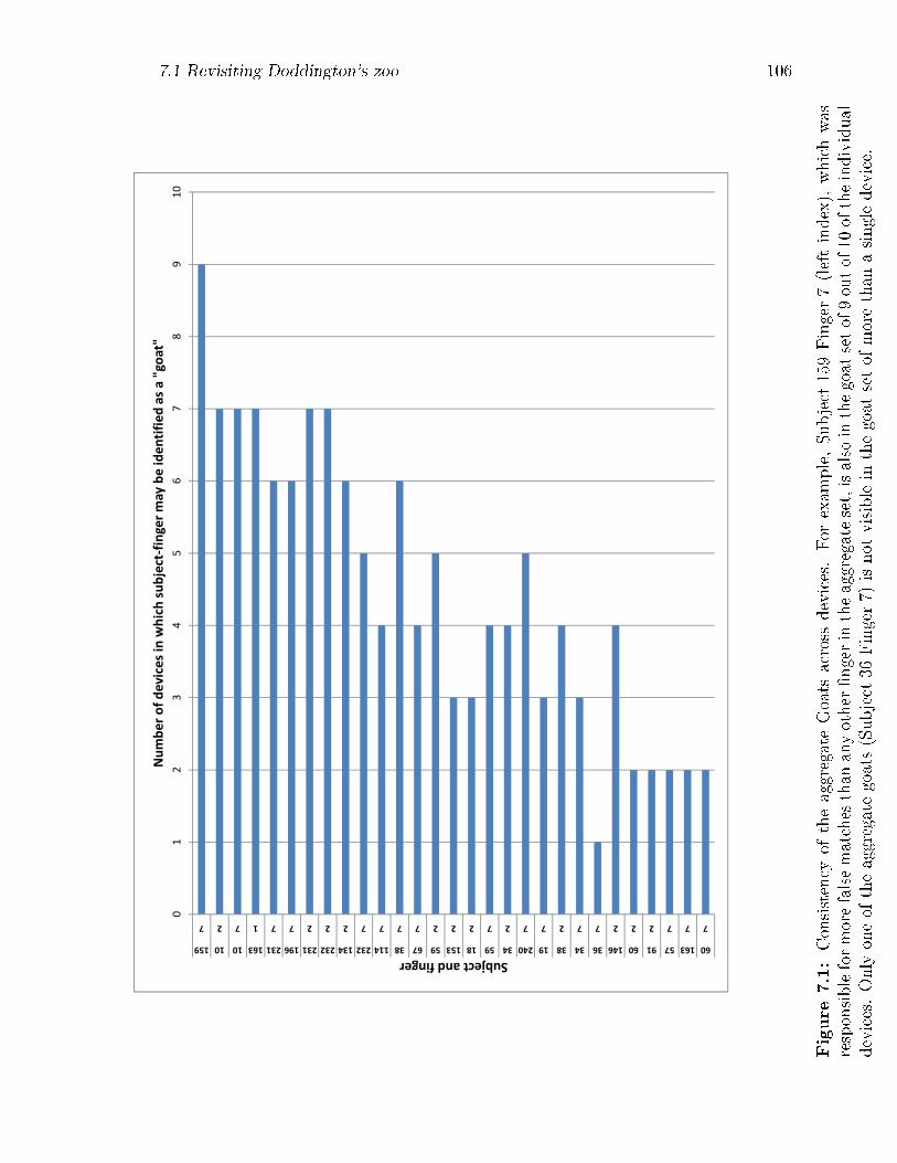
7.1 Revisiting Doddington's zoo 106
01
23
45
67
89
10
7 2 7 1 7 7 2 2 2 7 7 7 7 2 2 2 7 2 7 7 2 7 7 2 2 2 7 7 7
159 10 10 163 231 196 231 232 134 232 114 38 67 59 153 18 59 34 240 19 38 34 36 146 60 91 57 163 60
Nu
mb
er
of
de
vic
es
in w
hic
h s
ub
ject
-fin
ge
r m
ay
be
id
en
tifi
ed
as
a "
go
at"
Subject and finger
Figure
7.1:Consistency
oftheaggregateGoats
across
devices.For
exam
ple,Subject
159Finger7(leftindex),whichwas
responsibleformorefalsematchesthan
anyother�ngerintheaggregateset,isalso
inthegoat
setof9outof10
oftheindividual
devices.Only
oneof
theaggregategoats(Subject
36Finger7)
isnot
visiblein
thegoat
setof
morethan
asingledevice.
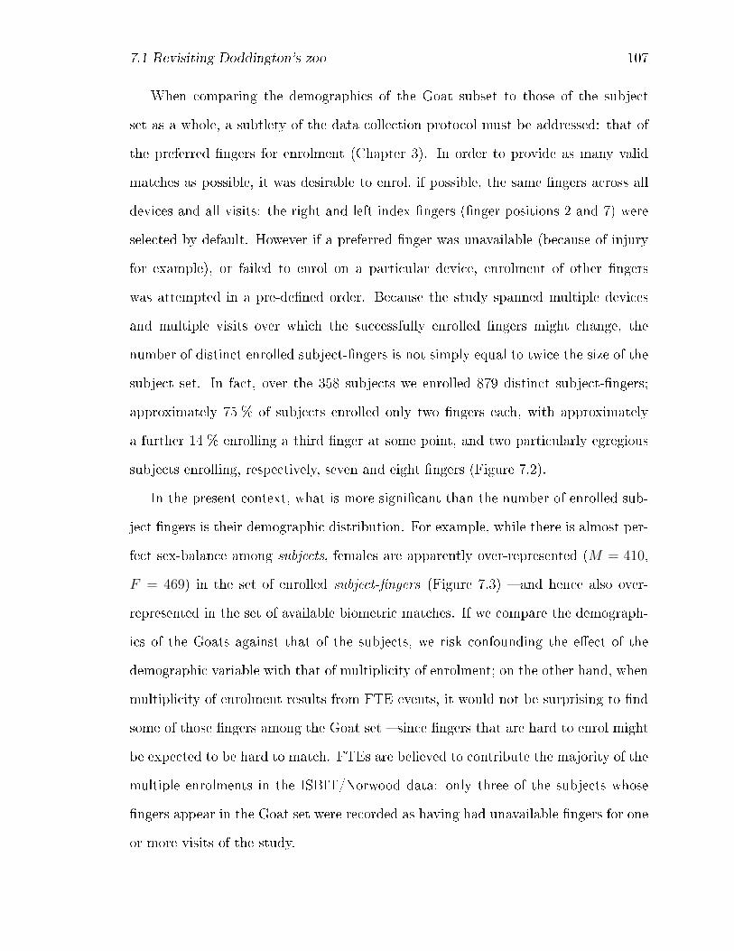
7.1 Revisiting Doddington's zoo 107
When comparing the demographics of the Goat subset to those of the subject
set as a whole, a subtlety of the data collection protocol must be addressed: that of
the preferred �ngers for enrolment (Chapter 3). In order to provide as many valid
matches as possible, it was desirable to enrol, if possible, the same �ngers across all
devices and all visits: the right and left index �ngers (�nger positions 2 and 7) were
selected by default. However if a preferred �nger was unavailable (because of injury
for example), or failed to enrol on a particular device, enrolment of other �ngers
was attempted in a pre-de�ned order. Because the study spanned multiple devices
and multiple visits over which the successfully enrolled �ngers might change, the
number of distinct enrolled subject-�ngers is not simply equal to twice the size of the
subject set. In fact, over the 358 subjects we enrolled 879 distinct subject-�ngers;
approximately 75 % of subjects enrolled only two �ngers each, with approximately
a further 14 % enrolling a third �nger at some point, and two particularly egregious
subjects enrolling, respectively, seven and eight �ngers (Figure 7.2).
In the present context, what is more signi�cant than the number of enrolled sub-
ject �ngers is their demographic distribution. For example, while there is almost per-
fect sex-balance among subjects, females are apparently over-represented (M = 410,
F = 469) in the set of enrolled subject-�ngers (Figure 7.3) � and hence also over-
represented in the set of available biometric matches. If we compare the demograph-
ics of the Goats against that of the subjects, we risk confounding the e�ect of the
demographic variable with that of multiplicity of enrolment; on the other hand, when
multiplicity of enrolment results from FTE events, it would not be surprising to �nd
some of those �ngers among the Goat set � since �ngers that are hard to enrol might
be expected to be hard to match. FTEs are believed to contribute the majority of the
multiple enrolments in the ISBIT/Norwood data: only three of the subjects whose
�ngers appear in the Goat set were recorded as having had unavailable �ngers for one
or more visits of the study.

7.1 Revisiting Doddington's zoo 108
0
50
100
150
200
250
300
2 3 4 5 6 7 8 9 10
Fre
qu
en
cy
Number of enrolled fingers
Figure 7.2: Distribution of numbers of enrolled �ngers per subject. Most subjects(approximately 75 %) enrolled just two �ngers over the course of the study, howevera few subjects enrolled additional �ngers as a result of unavailability of a previously-enrolled �nger, or failure to enrol a preferred �nger on a given device.
In the remainder of this section we use the demographics of the 879-member
enrolled subject-�nger set as the baseline for the comparisons.
Figures 7.4 � 7.7 show the empirical distributions of these demographics for the
aggregate Goat subset identi�ed in the preceding section, compared with the subject-
�nger cohort as a whole. We see compelling evidence that the Goats come predom-
inantly from the older individuals (birth years before 1970 - so aged at least 35-45
during the phases of the study) and predominantly from female subjects.
We may implement Fisher's exact test for signi�cance on the sex-imbalance of
the Goats as follows [35]. Suppose we are given a population of size N comprising
K females and N −K males. Under the null hypothesis H0, we pool the males and
females together and then select, randomly and without replacement, a sample of size
n, �nding that we have k females and n− k males. The probability mass function of
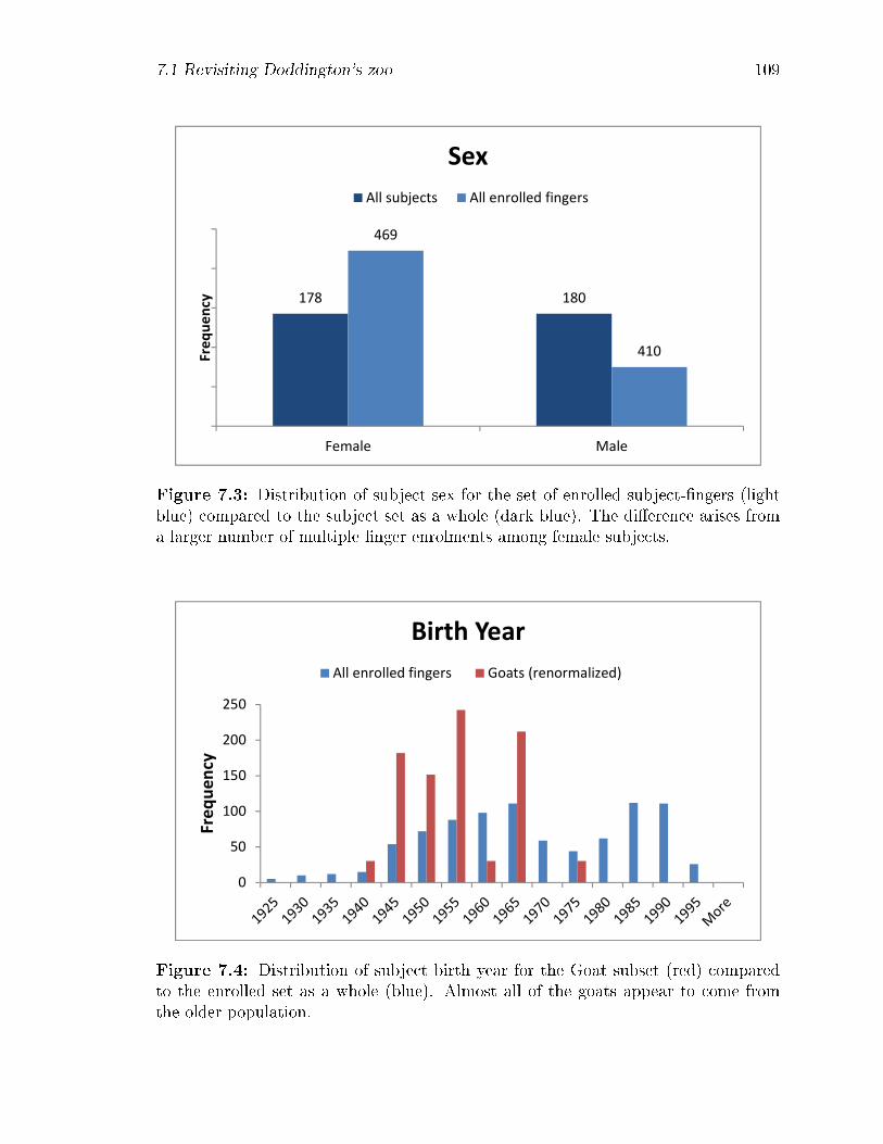
7.1 Revisiting Doddington's zoo 109
178 180
469
410
Female Male
Frequency
Sex
All subjects All enrolled fingers
Figure 7.3: Distribution of subject sex for the set of enrolled subject-�ngers (lightblue) compared to the subject set as a whole (dark blue). The di�erence arises froma larger number of multiple �nger enrolments among female subjects.
0
50
100
150
200
250
Fre
qu
en
cy
Birth Year
All enrolled fingers Goats (renormalized)
Figure 7.4: Distribution of subject birth year for the Goat subset (red) comparedto the enrolled set as a whole (blue). Almost all of the goats appear to come fromthe older population.
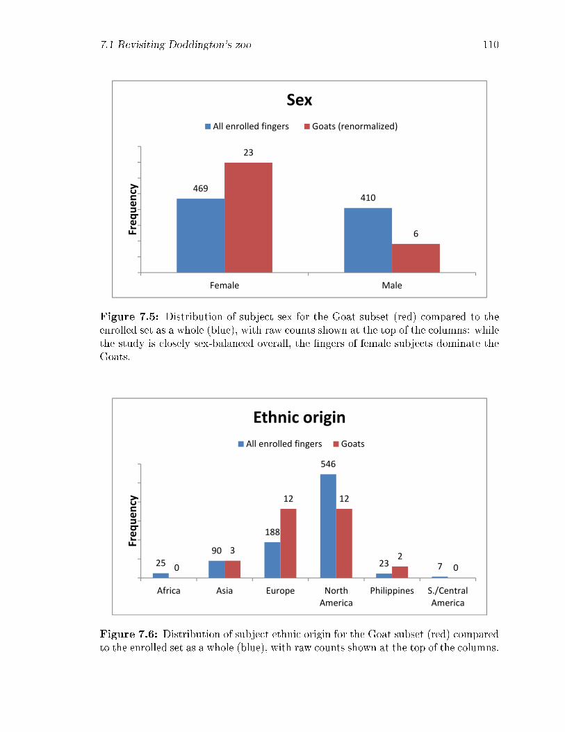
7.1 Revisiting Doddington's zoo 110
469410
23
6
Female Male
Frequency
Sex
All enrolled fingers Goats (renormalized)
Figure 7.5: Distribution of subject sex for the Goat subset (red) compared to theenrolled set as a whole (blue), with raw counts shown at the top of the columns: whilethe study is closely sex-balanced overall, the �ngers of female subjects dominate theGoats.
25
90
188
546
23 70
3
12 12
2
0
Africa Asia Europe North
America
Philippines S./Central
America
Fre
qu
en
cy
Ethnic origin
All enrolled fingers Goats
Figure 7.6: Distribution of subject ethnic origin for the Goat subset (red) comparedto the enrolled set as a whole (blue), with raw counts shown at the top of the columns.
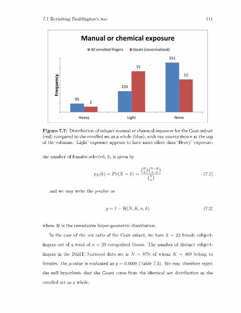
7.1 Revisiting Doddington's zoo 111
95
233
551
2
15
12
Heavy Light None
Fre
qu
en
cy
Manual or chemical exposure
All enrolled fingers Goats (renormalized)
Figure 7.7: Distribution of subject manual or chemical exposure for the Goat subset(red) compared to the enrolled set as a whole (blue), with raw counts shown at the topof the columns: `Light' exposure appears to have more e�ect than `Heavy' exposure.
the number of females selected, k, is given by
pX(k) = Pr(X = k) =
(Kk
)(N−Kn−k
)(Nn
) (7.1)
and we may write the p-value as
p = 1−H(N,K, n, k) (7.2)
where H is the cumulative hyper-geometric distribution.
In the case of the sex ratio of the Goat subset, we have k = 23 female subject-
�ngers out of a total of n = 29 categorized Goats. The number of distinct subject-
�ngers in the ISBIT/Norwood data set is N = 879, of whom K = 469 belong to
females: the p-value is evaluated as p = 0.0008 (Table 7.3). We may therefore reject
the null hypothesis that the Goats come from the identical sex distribution as the
enrolled set as a whole.
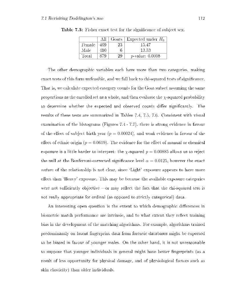
7.1 Revisiting Doddington's zoo 112
Table 7.3: Fisher exact test for the signi�cance of subject sex.
All Goats Expected under H0
Female 469 23 15.47Male 410 6 13.53Total 879 29 p-value: 0.0008
The other demographic variables each have more than two categories, making
exact tests of this form unfeasible, and we fall back to chi-squared tests of signi�cance.
That is, we calculate expected category counts for the Goat subset assuming the same
proportions as the enrolled set as a whole, and then evaluate the χ-squared probability
to determine whether the expected and observed counts di�er signi�cantly. The
results of these tests are summarized in Tables 7.4, 7.5, 7.6. Consistent with visual
examination of the histograms (Figures 7.4 - 7.7), there is strong evidence in favour
of the e�ect of subject birth year (p = 0.00024), and weak evidence in favour of the
e�ect of ethnic origin (p = 0.0619). The evidence for the e�ect of manual or chemical
exposure is a little harder to interpret: the χ-squared p = 0.00885 allows us to reject
the null at the Bonferroni-corrected signi�cance level α = 0.0125, however the exact
nature of the relationship is not clear, since `Light' exposure appears to have more
e�ect than `Heavy' exposure. This may be because the available exposure categories
were not su�ciently objective � or may re�ect the fact that the chi-squared test is
not really appropriate for ordinal (as opposed to strictly categorical) data.
An interesting open question is the extent to which demographic di�erences in
biometric match performance are intrinsic, and to what extent they re�ect training
bias in the development of the matching algorithms. For example, algorithms trained
predominantly on latent �ngerprint data from forensic databases might be expected
to be biased in favour of younger males. On the other hand, it is not unreasonable
to suppose that younger individuals in general might have better �ngerprints (as a
result of less opportunity for physical damage, and of physiological factors such as
skin elasticity) than older individuals.
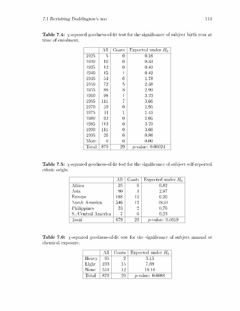
7.1 Revisiting Doddington's zoo 113
Table 7.4: χ-squared goodness-of-�t test for the signi�cance of subject birth year attime of enrolment.
All Goats Expected under H0
1925 5 0 0.161930 10 0 0.331935 12 0 0.401940 15 1 0.491945 54 6 1.781950 72 5 2.381955 88 8 2.901960 98 1 3.231965 111 7 3.661970 59 0 1.951975 44 1 1.451980 62 0 2.051985 112 0 3.701990 111 0 3.661995 26 0 0.86More 0 0 0.00Total 879 29 p-value: 0.00024
Table 7.5: χ-squared goodness-of-�t test for the signi�cance of subject self-reportedethnic origin.
All Goats Expected under H0
Africa 25 0 0.82Asia 90 3 2.97Europe 188 12 6.20North America 546 12 18.01Philippines 23 2 0.76S./Central America 7 0 0.23Total 879 29 p-value: 0.0619
Table 7.6: χ-squared goodness-of-�t test for the signi�cance of subject manual orchemical exposure.
All Goats Expected under H0
Heavy 95 2 3.13Light 233 15 7.69None 551 12 18.18Total 879 29 p-value: 0.0088
7.1 Revisiting Doddington's zoo 114
In addition to algorithm training, bias might be introduced at the feature extrac-
tion phase, either physically (for example, sensor devices whose size and resolution
is better matched to a speci�c demographic) or via the choice of which features to
extract for template generation.
7.1.3 NFIQ quality of the Goat subset
In the preceding Chapter, we considered the relationship between NFIQ quality and
overall classi�cation performance, but did not attempt to investigate whether low
quality is a more signi�cant factor for false matches or for false non-matches. Having
now identi�ed a subset of �ngers that contribute disproportionately to the FNMR,
we can approach the relationship from the other side and examine the relationship
more speci�cally between false non-matches and quality.
Figures 7.8 and 7.9 compare the mean NFIQ-1 and NFIQ-2 scores for the Goat
subset versus all subject-�ngers at enrolment and veri�cation, broken down by the
available devices. With the exception of Device H (whose NFIQ results we believe
to be erroneous) we observe consistently worse quality (NFIQ-1 higher and NFIQ-2
lower) amongst the Goats.
Although the set of Goat �ngers is relatively small (29), the sets of images for
which we have NFIQ scores are quite large, even when broken down by device. For
enrolment, there would be in the ideal case three images of each �nger for each of eight
visits, giving a total of 29× 24 = 696 samples per �nger per device3. In cases where
devices were removed in later visits the sets are somewhat smaller with the minimum
sample size being 328 images, for Device J. Veri�cation image sets are a factor two
larger since the protocol demands two veri�cation attempts, of three presentations
each. The baseline (all enrolled �nger) sets are substantially larger again - typically
around 9000 images per device for enrolment and 18,000 per device for veri�cation.
3The largest we see in practice is 648, because not all of the goats were enrolled at every visit onevery device
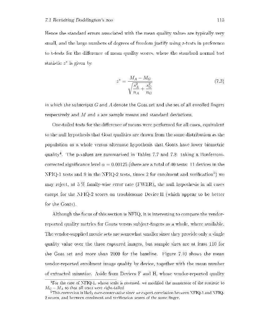
7.1 Revisiting Doddington's zoo 115
Hence the standard errors associated with the mean quality values are typically very
small, and the large numbers of degrees of freedom justify using z-tests in preference
to t-tests for the di�erence of mean quality scores, where the standard normal test
statistic z∗ is given by
z∗ =MA −MG√s2AnA
+s2GnG
(7.3)
in which the subscripts G and A denote the Goat set and the set of all enrolled �ngers
respectively and M and s are sample means and standard deviations.
One-tailed tests for the di�erence of means were performed for all cases, equivalent
to the null hypothesis that Goat qualities are drawn from the same distribution as the
population as a whole versus alternate hypothesis that Goats have lower biometric
quality4. The p-values are summarized in Tables 7.7 and 7.8: taking a Bonferroni-
corrected signi�cance level α = 0.00125 (there are a total of 40 tests: 11 devices in the
NFIQ-1 tests and 9 in the NFIQ-2 tests, times 2 for enrolment and veri�cation5) we
may reject, at 5 % family-wise error rate (FWER), the null hypothesis in all cases
except for the NFIQ-2 scores on troublesome Device H (which appear to be better
for the Goats).
Although the focus of this section is NFIQ, it is interesting to compare the vendor-
reported quality metrics for Goats versus subject-�ngers as a whole, where available.
The vendor-supplied metric sets are somewhat smaller since they provide only a single
quality value over the three captured images, but sample sizes are at least 110 for
the Goat set and more than 2000 for the baseline. Figure 7.10 shows the mean
vendor-reported enrolment image quality by device, together with the mean number
of extracted minutiae. Aside from Devices F and H, whose vendor-reported quality
4For the case of NFIQ-1, whose scale is reversed, we modi�ed the numerator of the statistic toMG −MA so that all tests were right-tailed
5This correction is likely over-conservative since we expect correlation between NFIQ-1 and NFIQ-2 scores, and between enrolment and veri�cation scores of the same �nger.
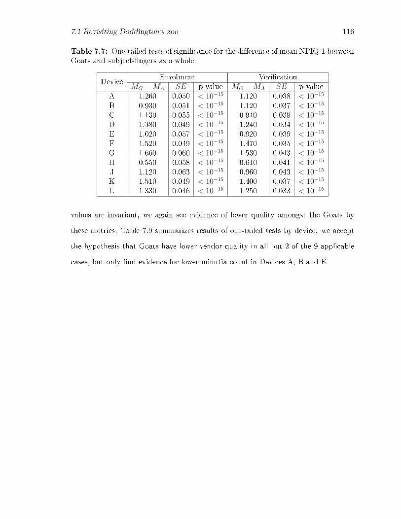
7.1 Revisiting Doddington's zoo 116
Table 7.7: One-tailed tests of signi�cance for the di�erence of mean NFIQ-1 betweenGoats and subject-�ngers as a whole.
DeviceEnrolment Veri�cation
MG −MA SE p-value MG −MA SE p-valueA 1.260 0.050 < 10−15 1.120 0.038 < 10−15
B 0.930 0.051 < 10−15 1.120 0.037 < 10−15
C 1.130 0.055 < 10−15 0.940 0.039 < 10−15
D 1.380 0.049 < 10−15 1.240 0.034 < 10−15
E 1.020 0.057 < 10−15 0.920 0.039 < 10−15
F 1.520 0.049 < 10−15 1.470 0.035 < 10−15
G 1.660 0.060 < 10−15 1.530 0.043 < 10−15
H 0.550 0.058 < 10−15 0.610 0.041 < 10−15
J 1.120 0.063 < 10−15 0.960 0.043 < 10−15
K 1.510 0.049 < 10−15 1.400 0.037 < 10−15
L 1.330 0.046 < 10−15 1.250 0.033 < 10−15
values are invariant, we again see evidence of lower quality amongst the Goats by
these metrics. Table 7.9 summarizes results of one-tailed tests by device: we accept
the hypothesis that Goats have lower vendor quality in all but 2 of the 9 applicable
cases, but only �nd evidence for lower minutia count in Devices A, B and E.

7.1 Revisiting Doddington's zoo 117
A B C D E F G H J K L
All 2.46 2.32 1.68 2.14 2.49 1.79 1.84 3.99 1.7 1.69 2.31
Goats 3.72 3.25 2.81 3.52 3.51 3.31 3.5 4.54 2.82 3.2 3.64
0
1
2
3
4
5
6
Me
an
NF
IQ1
sco
re
(a) Enrolment
A B C D E F G H J K L
All 2.33 2.3 1.54 2.02 2.39 1.69 1.71 3.93 1.55 1.63 2.28
Goats 3.45 3.42 2.48 3.26 3.31 3.16 3.24 4.54 2.51 3.03 3.53
0
1
2
3
4
5
6
Me
an
NF
IQ1
sco
re
(b) Veri�cation
Figure 7.8: Comparison of mean NFIQ1 score (lower = better quality) by devicefor the Goat subset (red) versus the enrolled set as a whole (blue). Error bars at ±1standard deviation for each device.

7.1 Revisiting Doddington's zoo 118
A B C D E F G H J K L
All 52 53 53 59 54 67 45 43 39
Goats 31 31 21 23 24 72 22 15 16
0
10
20
30
40
50
60
70
80
90
100
Me
an
NF
IQ2
sco
re
(a) Enrolment
A B C D E F G H J K L
All 51 54 55 60 56 67 47 44 39
Goats 29 32 24 24 26 72 23 16 17
0
10
20
30
40
50
60
70
80
90
100
Me
an
NF
IQ2
sco
re
(b) Veri�cation
Figure 7.9: Comparison of mean NFIQ2 score (higher = better quality) by devicefor the Goat subset (red) versus the enrolled set as a whole (blue). Error bars at ±1standard deviation for each device.
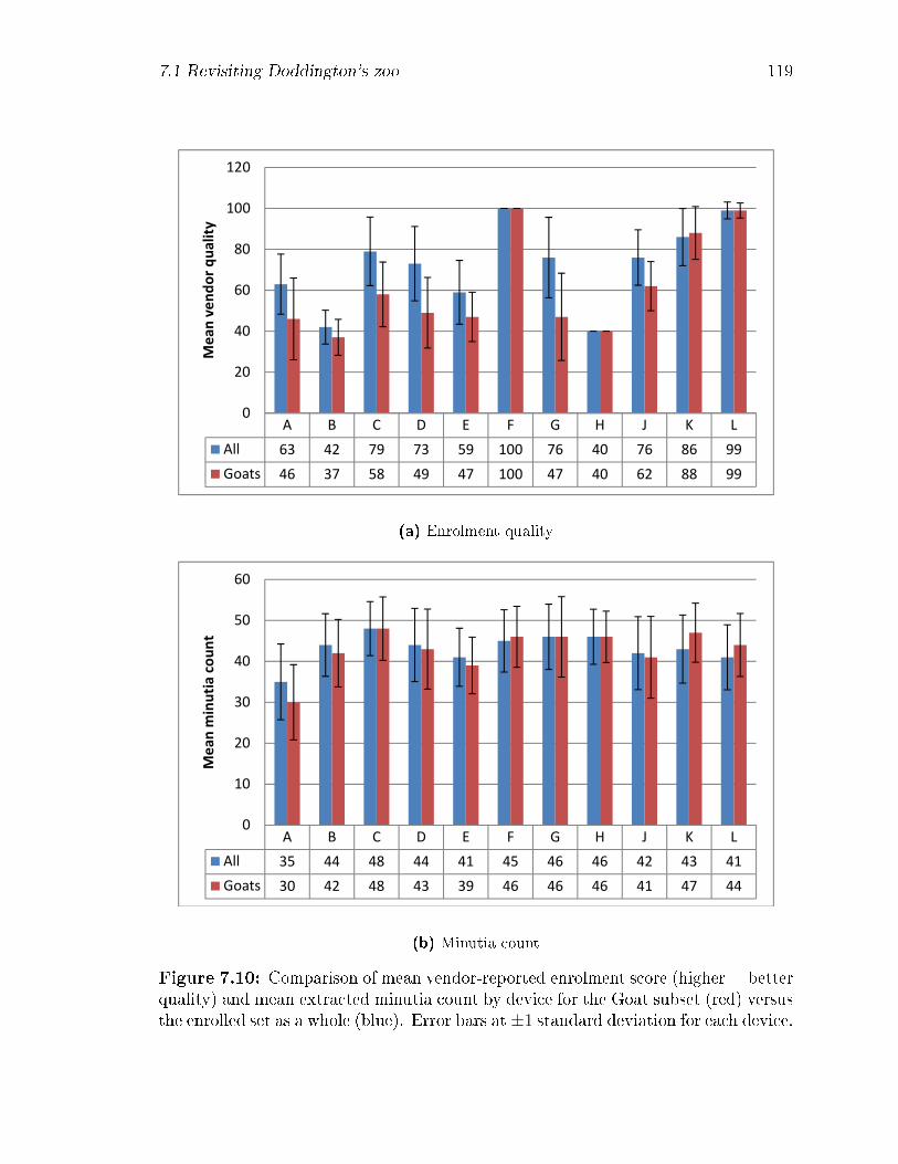
7.1 Revisiting Doddington's zoo 119
A B C D E F G H J K L
All 63 42 79 73 59 100 76 40 76 86 99
Goats 46 37 58 49 47 100 47 40 62 88 99
0
20
40
60
80
100
120
Me
an
ve
nd
or
qu
ali
ty
(a) Enrolment quality
A B C D E F G H J K L
All 35 44 48 44 41 45 46 46 42 43 41
Goats 30 42 48 43 39 46 46 46 41 47 44
0
10
20
30
40
50
60
Me
an
min
utia
co
un
t
(b) Minutia count
Figure 7.10: Comparison of mean vendor-reported enrolment score (higher = betterquality) and mean extracted minutia count by device for the Goat subset (red) versusthe enrolled set as a whole (blue). Error bars at ±1 standard deviation for each device.

7.1 Revisiting Doddington's zoo 120
Table 7.8: One-tailed tests of signi�cance for the di�erence of mean NFIQ-2 betweenGoats and subject-�ngers as a whole.
DeviceEnrolment Veri�cation
MA −MG SE p-value MA −MG SE p-valueA 0 N/A N/A 0 N/A N/AB 21 0.888 < 10−15 22 0.631 < 10−15
C 22 1.542 < 10−15 22 0.811 < 10−15
D 32 0.809 < 10−15 31 0.586 < 10−15
E 0 N/A N/A 0 N/A N/AF 36 1.106 < 10−15 36 0.717 < 10−15
G 30 1.046 < 10−15 30 0.687 < 10−15
H -5 0.369 1.000 -5 0.254 1.000J 23 1.757 < 10−15 24 0.796 < 10−15
K 28 0.642 < 10−15 28 0.477 < 10−15
L 23 0.593 < 10−15 22 0.428 < 10−15
Table 7.9: One-tailed tests of signi�cance for the di�erence of mean vendor-reportedenrolment image quality and minutia count between Goats and subject-�ngers as awhole.
DeviceVendor quality Minutia count
MG −MA SE p-value MG −MA SE p-valueA 17 1.518 < 10−15 5 0.737 5.74× 10⁻¹²
B 5 0.711 1.05× 10⁻¹² 2 0.669 0.001C 21 1.348 < 10−15 0 0.712 0.500D 24 1.232 < 10−15 1 0.750 0.091E 12 1.083 < 10−15 2 0.678 0.002F 0 0.000 N/A -1 0.508 0.975G 29 1.687 < 10−15 0 0.859 0.500H 0 0.000 N/A 0 0.493 0.500J 14 1.182 < 10−15 1 0.993 0.157K -2 0.920 0.985 -4 0.556 1.000L 0 0.261 0.5 -3 0.530 1.000

7.2 Wolves, Lambs and Sheep 121
7.2 Wolves, Lambs and Sheep
The enumeration of a Goat subset is relatively straightforward, since both enrolment
and veri�cation images come from the same individual. Doddington also attempted
to classify those matches that contribute disproportionately to the false match rate
(FMR), each in this case involving a pair of distinct individuals whom he labelled the
`Lamb' and the `Wolf' - the former being the preyed upon (impersonated) and the
latter the predator (impersonator). Implicit in this classi�cation is that the match
process be asymmetric [75].
We attempted to identify an aggregate Lamb-Wolf subset in the same way as
we did for the Goats: that is, with the same consideration as before of �nding a
reasonable operating point across all the available devices, choose a target FMR (in
our case, we chose 0.05 %), interpolate a set of decision thresholds for that FMR
across the various devices, and then �nd all the imposter match pairs whose scores
exceed those thresholds. Then aggregate the results across all devices by subject-
�nger, order them from largest to smallest number of false matches, and select the
subset accounting for 50 % of the total.
For the ISBIT-Norwood dataset, this results in a Lamb-Wolf subset of 2512 enrol-
verify subject-�nger pairs out of a total of 260719 imposter matches. Note that the
match software never attempts a �wrong �nger� match so, with a high probability,
these are all di�erent subject - same �nger matches6. The �rst thirty such match
pairs (ordered from highest to lowest aggregate number of false matches) are shown
in Table 7.10. Interestingly, the �rst two entries show exact symmetry i.e. they corre-
spond to false matches in which the same subject-�ngers, subject 291 and subject 167
�nger position 7 (left index), play the roles of Wolf and Lamb interchangeably.
Nevertheless, we may partition the Lamb-Wolf set according to which role each
6Although �ngers would, as a result of subject and/or operator inattention, infrequently bemislabelled during enrolment or veri�cation, manual scrubbing of each day's data acquisition by anexperienced supervisor is believed to have substantially removed these mislabellings

7.2 Wolves, Lambs and Sheep 122
56 85
Wolves 513
Lambs 480
Goats 29
1 5
16
7
407
Figure 7.11: Venn diagram illustrating the overlap between the identi�ed Goats,Lambs, and Wolves. By elimination, 302 of the 879 subject-�ngers are not within theunion of the sets and may thus be identi�ed as Sheep.
subject-�nger plays in the match, reducing the 2512 Lamb-Wolf match pairs to sets of
480 distinct Lamb subject-�ngers and 513 distinct Wolf subject-�ngers respectively.
The overlap between Goats, Lambs, and Wolves is represented graphically in Fig-
ure 7.11. By elimination, 302 of the 879 subject-�ngers are not within the union of
the sets and may thus be identi�ed in Doddington's classi�cation as Sheep.
7.2.1 Demographics of the Lamb and Wolf subsets
Since the Lamb and Wolf subsets identi�ed in the preceding section substantially
sample the entire set of enrolled subject �ngers (representing respectively 480 and
513 of the 879 distinct subject-�ngers), we would not expect demographic di�erences
to so pronounced as for the much smaller Goat subset. However we include the
demographic analysis here for completeness (Figures 7.12 - 7.15). A Fisher exact test
was performed as before for the sex distributions - while the Lambs show essentially
no evidence of an e�ect (p = 0.47) there is a small amount of evidence that males
are over-represented among the Wolves - that is, with a post-hoc assignment of males
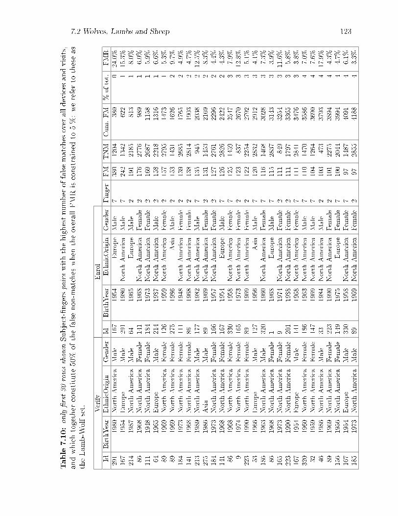
7.2 Wolves, Lambs and Sheep 123
Table7.10:only�rst30
rowsshow
nSubject-�ngerspairswiththehighestnumber
offalsematches
over
alldevices
andvisits,
andwhichtogether
constitute
50%
ofthefalsenon-m
atches
when
theoverallFMRisconstrained
to5%:wereferto
theseas
theLam
b-W
olfset. Verify
Enrol
IdBirthYear
EthnicOrigin
Gender
IdBirthYear
EthnicOrigin
Gender
Finger
FM
TNM
Cum.FM
%of
tot.
FMR
291
1980
North
America
Male
167
1954
Europe
Male
7380
1204
380
024.0%
167
1954
Europe
Male
291
1980
North
America
Male
7242
1342
622
115.3%
214
1987
North
America
Male
641965
Europe
Male
2191
2185
813
18.0%
861968
North
America
Fem
ale
141
1968
North
America
Fem
ale
2176
2776
989
16.0%
111
1948
North
America
Fem
ale
184
1973
North
America
Fem
ale
2169
2687
1158
15.9%
641965
Europe
Male
214
1987
North
America
Male
2158
2218
1316
16.6%
891969
North
America
Fem
ale
126
1959
North
America
Fem
ale
2157
2795
1473
15.3%
891969
North
America
Fem
ale
275
1986
Asia
Male
2153
1431
1626
29.7%
184
1973
North
America
Fem
ale
111
1948
North
America
Fem
ale
2139
2685
1765
24.9%
141
1968
North
America
Fem
ale
861968
North
America
Fem
ale
2138
2814
1903
24.7%
213
1989
North
America
Male
177
1982
North
America
Male
7135
945
2038
212.5%
275
1986
Asia
Male
891969
North
America
Fem
ale
2131
1453
2169
28.3%
184
1973
North
America
Fem
ale
166
1957
North
America
Fem
ale
2127
2761
2296
24.4%
141
1968
North
America
Fem
ale
167
1954
Europe
Male
7126
2826
2422
24.3%
861968
North
America
Fem
ale
330
1958
North
America
Fem
ale
7125
1459
2547
37.9%
91974
North
America
Fem
ale
165
1973
North
America
Fem
ale
2123
837
2670
312.8%
223
1990
North
America
Fem
ale
891969
North
America
Fem
ale
2122
2254
2792
35.1%
531966
Europe
Male
127
1956
Asia
Male
7120
2832
2912
34.1%
186
1963
North
America
Male
320
1960
North
America
Fem
ale
7116
1468
3028
37.3%
861968
North
America
Fem
ale
11968
Europe
Male
7115
2837
3143
33.9%
165
1973
North
America
Fem
ale
91974
North
America
Fem
ale
2111
849
3254
311.6%
223
1990
North
America
Fem
ale
201
1988
North
America
Fem
ale
2111
1797
3365
35.8%
167
1954
Europe
Male
141
1968
North
America
Fem
ale
7111
2841
3476
33.8%
320
1960
North
America
Fem
ale
186
1963
North
America
Male
7110
1470
3586
47.0%
321959
North
America
Fem
ale
147
1969
North
America
Male
7104
1264
3690
47.6%
461986
North
America
Male
331984
North
America
Male
2103
473
3793
417.9%
891969
North
America
Fem
ale
223
1990
North
America
Fem
ale
2101
2275
3894
44.3%
156
1956
North
America
Fem
ale
149
1975
Europe
Fem
ale
7100
2044
3994
44.7%
167
1954
Europe
Male
330
1958
North
America
Fem
ale
797
1487
4091
46.1%
185
1973
North
America
Male
891969
North
America
Fem
ale
297
2855
4188
43.3%
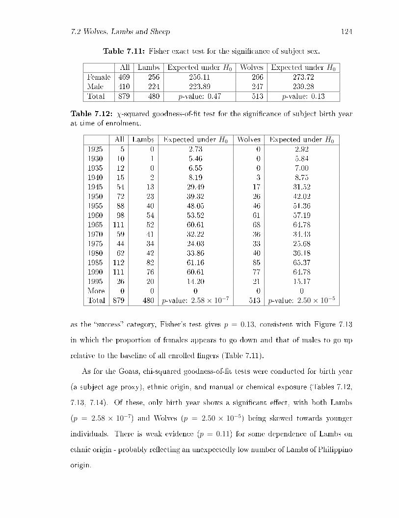
7.2 Wolves, Lambs and Sheep 124
Table 7.11: Fisher exact test for the signi�cance of subject sex.
All Lambs Expected under H0 Wolves Expected under H0
Female 469 256 256.11 266 273.72Male 410 224 223.89 247 239.28Total 879 480 p-value: 0.47 513 p-value: 0.13
Table 7.12: χ-squared goodness-of-�t test for the signi�cance of subject birth yearat time of enrolment.
All Lambs Expected under H0 Wolves Expected under H0
1925 5 0 2.73 0 2.921930 10 1 5.46 0 5.841935 12 0 6.55 0 7.001940 15 2 8.19 3 8.751945 54 13 29.49 17 31.521950 72 23 39.32 26 42.021955 88 40 48.05 46 51.361960 98 54 53.52 61 57.191965 111 52 60.61 68 64.781970 59 41 32.22 36 34.431975 44 34 24.03 33 25.681980 62 42 33.86 40 36.181985 112 82 61.16 85 65.371990 111 76 60.61 77 64.781995 26 20 14.20 21 15.17More 0 0 0 0 0Total 879 480 p-value: 2.58× 10⁻⁷ 513 p-value: 2.50× 10⁻⁵
as the �success� category, Fisher's test gives p = 0.13, consistent with Figure 7.13
in which the proportion of females appears to go down and that of males to go up
relative to the baseline of all enrolled �ngers (Table 7.11).
As for the Goats, chi-squared goodness-of-�t tests were conducted for birth year
(a subject age proxy), ethnic origin, and manual or chemical exposure (Tables 7.12,
7.13, 7.14). Of these, only birth year shows a signi�cant e�ect, with both Lambs
(p = 2.58 × 10⁻⁷) and Wolves (p = 2.50 × 10⁻⁵) being skewed towards younger
individuals. There is weak evidence (p = 0.11) for some dependence of Lambs on
ethnic origin - probably re�ecting an unexpectedly low number of Lambs of Philippino
origin.
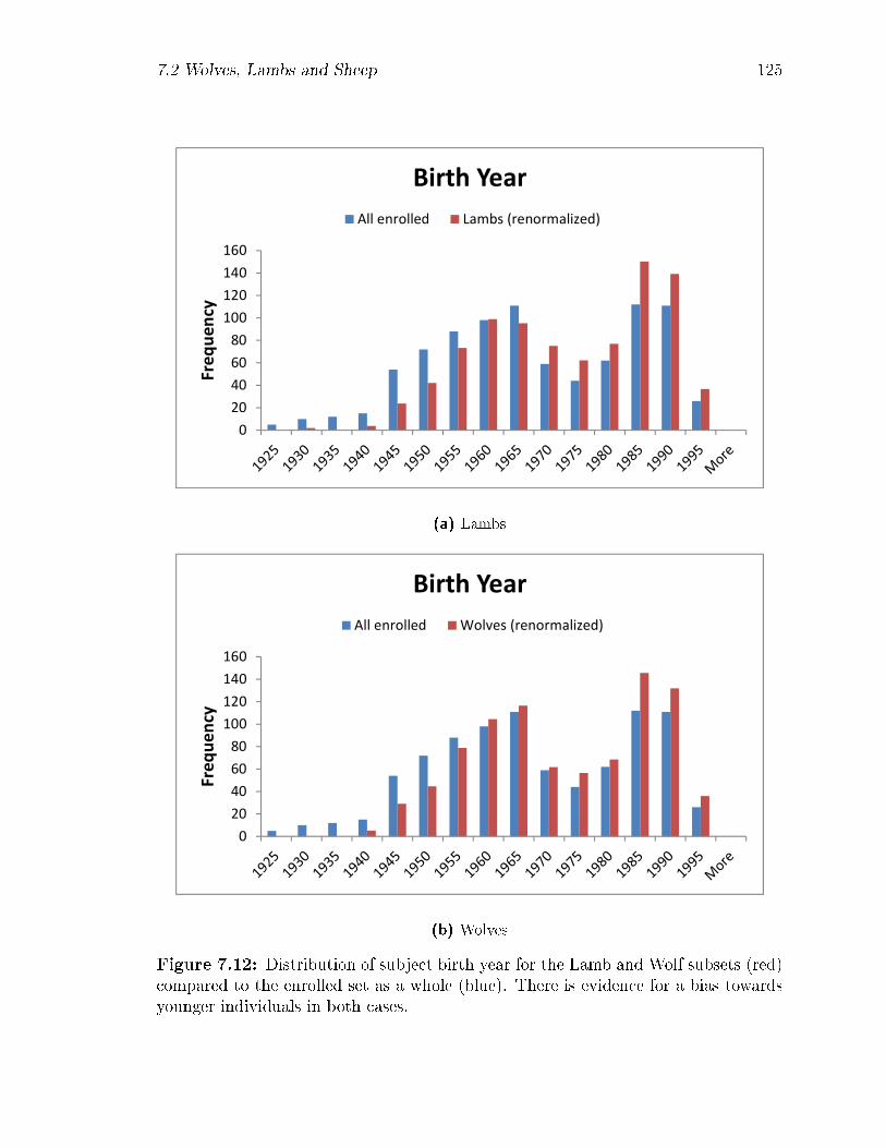
7.2 Wolves, Lambs and Sheep 125
0
20
40
60
80
100
120
140
160
Fre
qu
en
cy
Birth Year
All enrolled Lambs (renormalized)
(a) Lambs
0
20
40
60
80
100
120
140
160
Fre
qu
en
cy
Birth Year
All enrolled Wolves (renormalized)
(b) Wolves
Figure 7.12: Distribution of subject birth year for the Lamb and Wolf subsets (red)compared to the enrolled set as a whole (blue). There is evidence for a bias towardsyounger individuals in both cases.
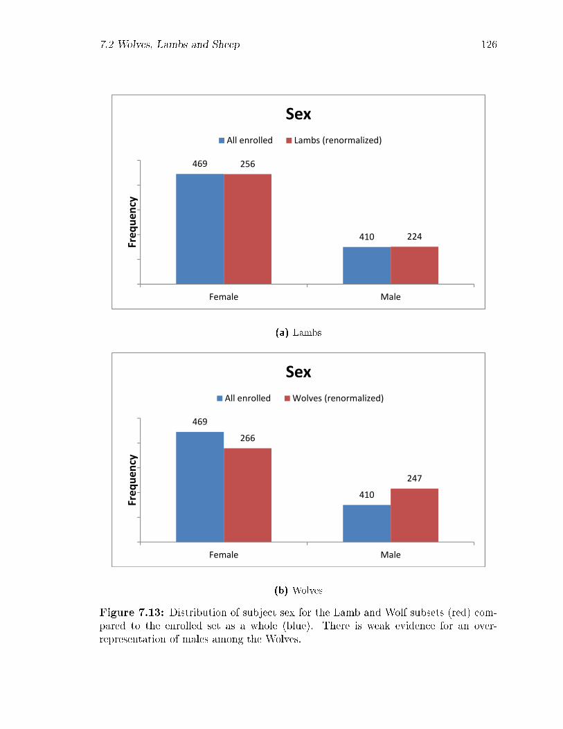
7.2 Wolves, Lambs and Sheep 126
469
410
256
224
Female Male
Frequency
Sex
All enrolled Lambs (renormalized)
(a) Lambs
469
410
266
247
Female Male
Frequency
Sex
All enrolled Wolves (renormalized)
(b) Wolves
Figure 7.13: Distribution of subject sex for the Lamb and Wolf subsets (red) com-pared to the enrolled set as a whole (blue). There is weak evidence for an over-representation of males among the Wolves.

7.2 Wolves, Lambs and Sheep 127
25
90
188
546
23 715
54
93
308
4 6
Africa Asia Europe North
America
Philippines S./Central
America
Fre
qu
en
cy
Ethnic origin
Series1 Lambs (renormalized)
(a) Lambs
25
90
188
546
23 716
58
103
322
8 6
Africa Asia Europe North
America
Philippines S./Central
America
Fre
qu
en
cy
Ethnic origin
All enrolled Wolves (renormalized)
(b) Wolves
Figure 7.14: Distribution of subject ethnic origin for the Lamb and Wolf subsets(red) compared to the enrolled set as a whole (blue). There is little evidence of ane�ect.
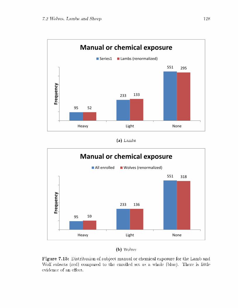
7.2 Wolves, Lambs and Sheep 128
95
233
551
52
133
295
Heavy Light None
Fre
qu
en
cy
Manual or chemical exposure
Series1 Lambs (renormalized)
(a) Lambs
95
233
551
59
136
318
Heavy Light None
Fre
qu
en
cy
Manual or chemical exposure
All enrolled Wolves (renormalized)
(b) Wolves
Figure 7.15: Distribution of subject manual or chemical exposure for the Lamb andWolf subsets (red) compared to the enrolled set as a whole (blue). There is littleevidence of an e�ect.
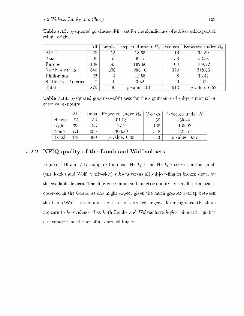
7.2 Wolves, Lambs and Sheep 129
Table 7.13: χ-squared goodness-of-�t test for the signi�cance of subject self-reportedethnic origin.
All Lambs Expected under H0 Wolves Expected under H0
Africa 25 15 13.65 16 14.59Asia 90 54 49.15 58 52.53Europe 188 93 102.66 103 109.72North America 546 308 298.16 322 318.66Philippines 23 4 12.56 8 13.42S./Central America 7 6 3.82 6 4.09Total 879 480 p-value: 0.11 513 p-value: 0.52
Table 7.14: χ-squared goodness-of-�t test for the signi�cance of subject manual orchemical exposure.
All Lambs Expected under H0 Wolves Expected under H0
Heavy 95 52 51.88 59 55.44Light 233 133 127.24 136 135.98None 551 295 300.89 318 321.57Total 879 480 p-value: 0.83 513 p-value: 0.87
7.2.2 NFIQ quality of the Lamb and Wolf subsets
Figures 7.16 and 7.17 compare the mean NFIQ-1 and NFIQ-2 scores for the Lamb
(enrol-side) and Wolf (verify-side) subsets versus all subject-�ngers broken down by
the available devices. The di�erences in mean biometric quality are smaller than those
observed in the Goats, as one might expect given the much greater overlap between
the Lamb/Wolf subsets and the set of all enrolled �ngers. More signi�cantly, there
appears to be evidence that both Lambs and Wolves have higher biometric quality
on average than the set of all enrolled �ngers.
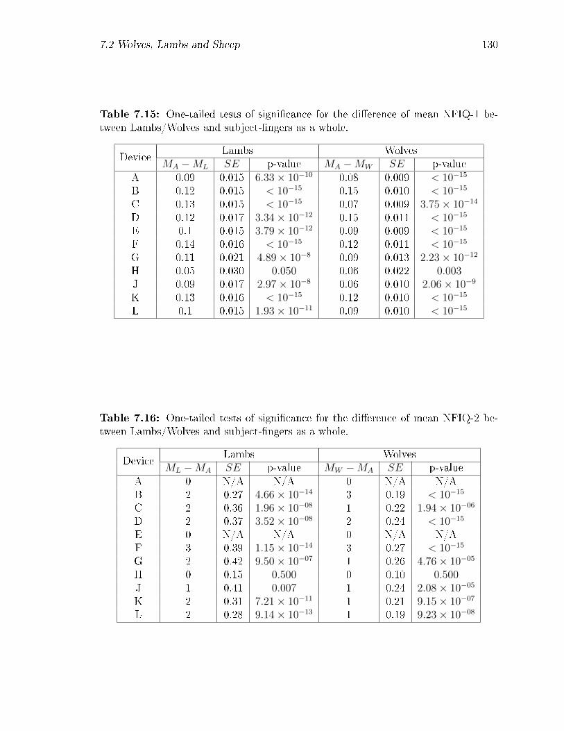
7.2 Wolves, Lambs and Sheep 130
Table 7.15: One-tailed tests of signi�cance for the di�erence of mean NFIQ-1 be-tween Lambs/Wolves and subject-�ngers as a whole.
DeviceLambs Wolves
MA −ML SE p-value MA −MW SE p-valueA 0.09 0.015 6.33× 10⁻¹⁰ 0.08 0.009 < 10−15
B 0.12 0.015 < 10−15 0.15 0.010 < 10−15
C 0.13 0.015 < 10−15 0.07 0.009 3.75× 10⁻¹⁴
D 0.12 0.017 3.34× 10⁻¹² 0.15 0.011 < 10−15
E 0.1 0.015 3.79× 10⁻¹² 0.09 0.009 < 10−15
F 0.14 0.016 < 10−15 0.12 0.011 < 10−15
G 0.11 0.021 4.89× 10⁻⁸ 0.09 0.013 2.23× 10⁻¹²
H 0.05 0.030 0.050 0.06 0.022 0.003J 0.09 0.017 2.97× 10⁻⁸ 0.06 0.010 2.06× 10⁻⁹
K 0.13 0.016 < 10−15 0.12 0.010 < 10−15
L 0.1 0.015 1.93× 10⁻¹¹ 0.09 0.010 < 10−15
Table 7.16: One-tailed tests of signi�cance for the di�erence of mean NFIQ-2 be-tween Lambs/Wolves and subject-�ngers as a whole.
DeviceLambs Wolves
ML −MA SE p-value MW −MA SE p-valueA 0 N/A N/A 0 N/A N/AB 2 0.27 4.66× 10⁻¹⁴ 3 0.19 < 10−15
C 2 0.36 1.96× 10−08 1 0.22 1.94× 10−06
D 2 0.37 3.52× 10−08 2 0.24 < 10−15
E 0 N/A N/A 0 N/A N/AF 3 0.39 1.15× 10⁻¹⁴ 3 0.27 < 10−15
G 2 0.42 9.50× 10−07 1 0.26 4.76× 10−05
H 0 0.15 0.500 0 0.10 0.500J 1 0.41 0.007 1 0.24 2.08× 10−05
K 2 0.31 7.21× 10⁻¹¹ 1 0.21 9.15× 10−07
L 2 0.28 9.14× 10⁻¹³ 1 0.19 9.23× 10−08

7.2 Wolves, Lambs and Sheep 131
A B C D E F G H J K L
All 2.46 2.32 1.68 2.14 2.49 1.79 1.84 3.99 1.7 1.69 2.31
Lambs 2.37 2.2 1.55 2.02 2.39 1.65 1.73 3.94 1.61 1.56 2.21
0
1
2
3
4
5
6
Me
an
NF
IQ1
sco
re
(a) Lambs
A B C D E F G H J K L
All 2.33 2.3 1.54 2.02 2.39 1.69 1.71 3.93 1.55 1.63 2.28
Wolves 2.25 2.15 1.47 1.87 2.3 1.57 1.62 3.87 1.49 1.51 2.19
0
1
2
3
4
5
6
Me
an
NF
IQ1
sco
re
(b) Wolves
Figure 7.16: Comparison of mean NFIQ1 score (lower = better quality) by devicefor the Lamb and Wolf subsets (red) versus the enrolled set as a whole (blue). Errorbars at ±1 standard deviation for each device.
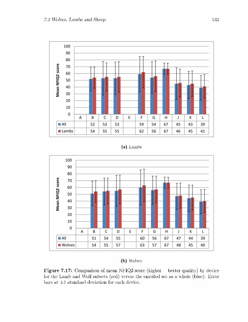
7.2 Wolves, Lambs and Sheep 132
A B C D E F G H J K L
All 52 53 53 59 54 67 45 43 39
Lambs 54 55 55 62 56 67 46 45 41
0
10
20
30
40
50
60
70
80
90
100
Me
an
NF
IQ2
sco
re
(a) Lambs
A B C D E F G H J K L
All 51 54 55 60 56 67 47 44 39
Wolves 54 55 57 63 57 67 48 45 40
0
10
20
30
40
50
60
70
80
90
100
Me
an
NF
IQ2
sco
re
(b) Wolves
Figure 7.17: Comparison of mean NFIQ2 score (higher = better quality) by devicefor the Lamb and Wolf subsets (red) versus the enrolled set as a whole (blue). Errorbars at ±1 standard deviation for each device.
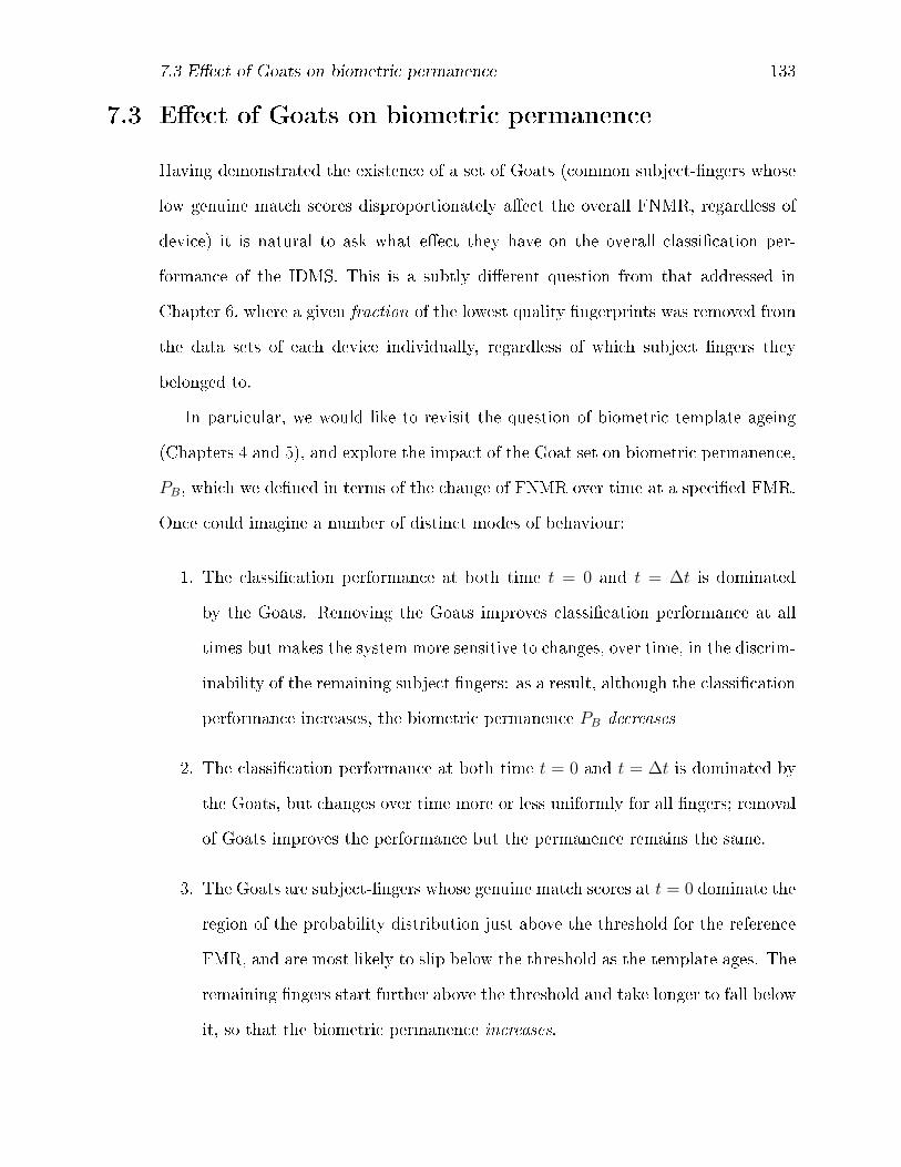
7.3 E�ect of Goats on biometric permanence 133
7.3 E�ect of Goats on biometric permanence
Having demonstrated the existence of a set of Goats (common subject-�ngers whose
low genuine match scores disproportionately a�ect the overall FNMR, regardless of
device) it is natural to ask what e�ect they have on the overall classi�cation per-
formance of the IDMS. This is a subtly di�erent question from that addressed in
Chapter 6, where a given fraction of the lowest quality �ngerprints was removed from
the data sets of each device individually, regardless of which subject �ngers they
belonged to.
In particular, we would like to revisit the question of biometric template ageing
(Chapters 4 and 5), and explore the impact of the Goat set on biometric permanence,
PB, which we de�ned in terms of the change of FNMR over time at a speci�ed FMR.
Once could imagine a number of distinct modes of behaviour:
1. The classi�cation performance at both time t = 0 and t = ∆t is dominated
by the Goats. Removing the Goats improves classi�cation performance at all
times but makes the system more sensitive to changes, over time, in the discrim-
inability of the remaining subject �ngers: as a result, although the classi�cation
performance increases, the biometric permanence PB decreases
2. The classi�cation performance at both time t = 0 and t = ∆t is dominated by
the Goats, but changes over time more or less uniformly for all �ngers; removal
of Goats improves the performance but the permanence remains the same.
3. The Goats are subject-�ngers whose genuine match scores at t = 0 dominate the
region of the probability distribution just above the threshold for the reference
FMR, and are most likely to slip below the threshold as the template ages. The
remaining �ngers start further above the threshold and take longer to fall below
it, so that the biometric permanence increases.
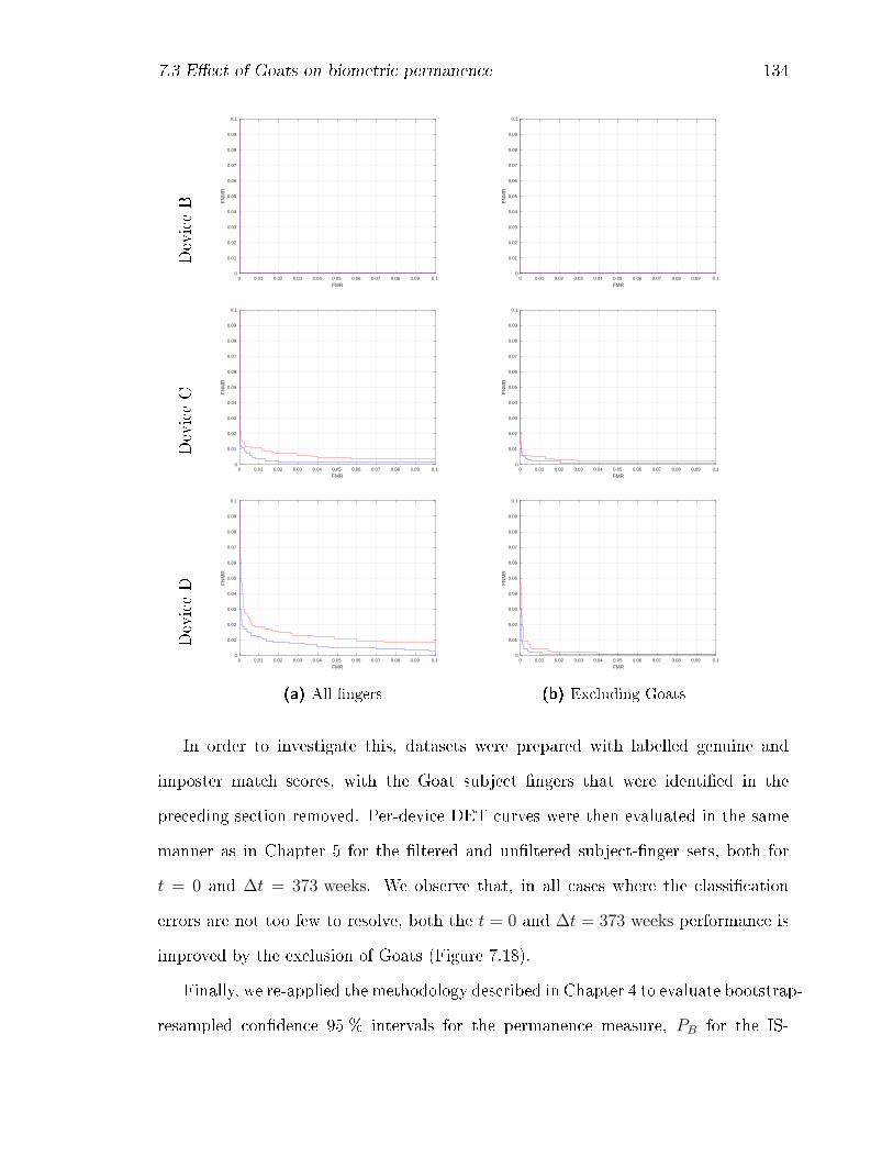
7.3 E�ect of Goats on biometric permanence 134
DeviceB
0 0.01 0.02 0.03 0.04 0.05 0.06 0.07 0.08 0.09 0.1
FMR
0
0.01
0.02
0.03
0.04
0.05
0.06
0.07
0.08
0.09
0.1
FN
MR
DeviceC
0 0.01 0.02 0.03 0.04 0.05 0.06 0.07 0.08 0.09 0.1
FMR
0
0.01
0.02
0.03
0.04
0.05
0.06
0.07
0.08
0.09
0.1
FN
MR
DeviceD
0 0.01 0.02 0.03 0.04 0.05 0.06 0.07 0.08 0.09 0.1
FMR
0
0.01
0.02
0.03
0.04
0.05
0.06
0.07
0.08
0.09
0.1
FN
MR
(a) All �ngers
0 0.01 0.02 0.03 0.04 0.05 0.06 0.07 0.08 0.09 0.1
FMR
0
0.01
0.02
0.03
0.04
0.05
0.06
0.07
0.08
0.09
0.1
FN
MR
0 0.01 0.02 0.03 0.04 0.05 0.06 0.07 0.08 0.09 0.1
FMR
0
0.01
0.02
0.03
0.04
0.05
0.06
0.07
0.08
0.09
0.1
FN
MR
0 0.01 0.02 0.03 0.04 0.05 0.06 0.07 0.08 0.09 0.1
FMR
0
0.01
0.02
0.03
0.04
0.05
0.06
0.07
0.08
0.09
0.1F
NM
R
(b) Excluding Goats
In order to investigate this, datasets were prepared with labelled genuine and
imposter match scores, with the Goat subject �ngers that were identi�ed in the
preceding section removed. Per-device DET curves were then evaluated in the same
manner as in Chapter 5 for the �ltered and un�ltered subject-�nger sets, both for
t = 0 and ∆t = 373 weeks. We observe that, in all cases where the classi�cation
errors are not too few to resolve, both the t = 0 and ∆t = 373 weeks performance is
improved by the exclusion of Goats (Figure 7.18).
Finally, we re-applied the methodology described in Chapter 4 to evaluate bootstrap-
resampled con�dence 95 % intervals for the permanence measure, PB for the IS-
7.3 E�ect of Goats on biometric permanence 135
DeviceF
0 0.01 0.02 0.03 0.04 0.05 0.06 0.07 0.08 0.09 0.1
FMR
0
0.01
0.02
0.03
0.04
0.05
0.06
0.07
0.08
0.09
0.1
FN
MR
DeviceG
0 0.01 0.02 0.03 0.04 0.05 0.06 0.07 0.08 0.09 0.1
FMR
0
0.01
0.02
0.03
0.04
0.05
0.06
0.07
0.08
0.09
0.1
FN
MR
DeviceH
0 0.01 0.02 0.03 0.04 0.05 0.06 0.07 0.08 0.09 0.1
FMR
0
0.01
0.02
0.03
0.04
0.05
0.06
0.07
0.08
0.09
0.1
FN
MR
(a) All �ngers
0 0.01 0.02 0.03 0.04 0.05 0.06 0.07 0.08 0.09 0.1
FMR
0
0.01
0.02
0.03
0.04
0.05
0.06
0.07
0.08
0.09
0.1
FN
MR
0 0.01 0.02 0.03 0.04 0.05 0.06 0.07 0.08 0.09 0.1
FMR
0
0.01
0.02
0.03
0.04
0.05
0.06
0.07
0.08
0.09
0.1
FN
MR
0 0.01 0.02 0.03 0.04 0.05 0.06 0.07 0.08 0.09 0.1
FMR
0
0.01
0.02
0.03
0.04
0.05
0.06
0.07
0.08
0.09
0.1
FN
MR
(b) Excluding Goats
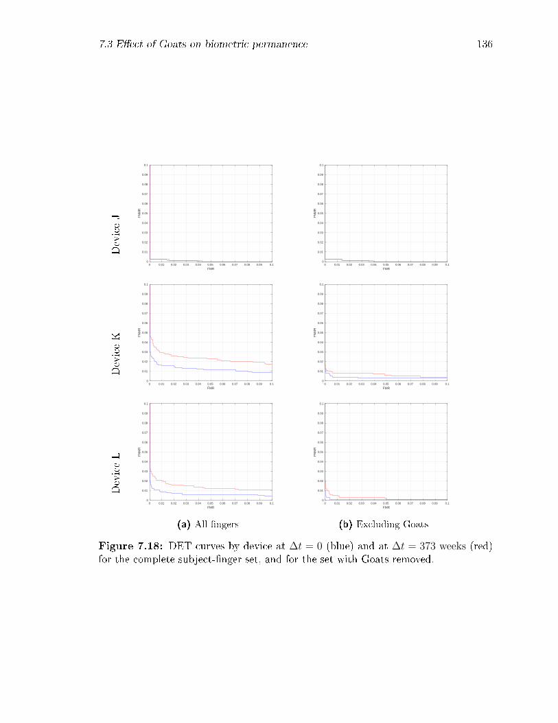
7.3 E�ect of Goats on biometric permanence 136
DeviceJ
0 0.01 0.02 0.03 0.04 0.05 0.06 0.07 0.08 0.09 0.1
FMR
0
0.01
0.02
0.03
0.04
0.05
0.06
0.07
0.08
0.09
0.1
FN
MR
DeviceK
0 0.01 0.02 0.03 0.04 0.05 0.06 0.07 0.08 0.09 0.1
FMR
0
0.01
0.02
0.03
0.04
0.05
0.06
0.07
0.08
0.09
0.1
FN
MR
DeviceL
0 0.01 0.02 0.03 0.04 0.05 0.06 0.07 0.08 0.09 0.1
FMR
0
0.01
0.02
0.03
0.04
0.05
0.06
0.07
0.08
0.09
0.1
FN
MR
(a) All �ngers
0 0.01 0.02 0.03 0.04 0.05 0.06 0.07 0.08 0.09 0.1
FMR
0
0.01
0.02
0.03
0.04
0.05
0.06
0.07
0.08
0.09
0.1
FN
MR
0 0.01 0.02 0.03 0.04 0.05 0.06 0.07 0.08 0.09 0.1
FMR
0
0.01
0.02
0.03
0.04
0.05
0.06
0.07
0.08
0.09
0.1
FN
MR
0 0.01 0.02 0.03 0.04 0.05 0.06 0.07 0.08 0.09 0.1
FMR
0
0.01
0.02
0.03
0.04
0.05
0.06
0.07
0.08
0.09
0.1
FN
MR
(b) Excluding Goats
Figure 7.18: DET curves by device at ∆t = 0 (blue) and at ∆t = 373 weeks (red)for the complete subject-�nger set, and for the set with Goats removed.
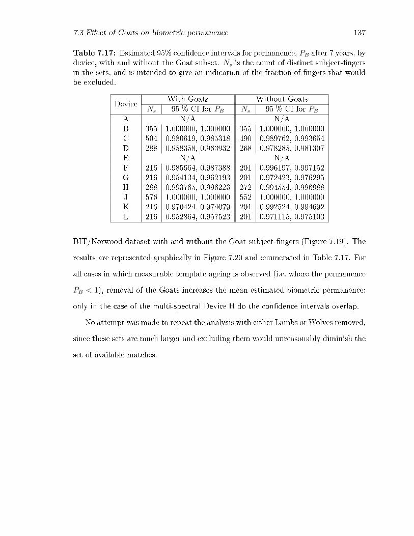
7.3 E�ect of Goats on biometric permanence 137
Table 7.17: Estimated 95% con�dence intervals for permanence, PB after 7 years, bydevice, with and without the Goat subset. Ns is the count of distinct subject-�ngersin the sets, and is intended to give an indication of the fraction of �ngers that wouldbe excluded.
DeviceWith Goats Without Goats
Ns 95 % CI for PB Ns 95 % CI for PB
A N/A N/AB 355 1.000000, 1.000000 355 1.000000, 1.000000C 504 0.980619, 0.985318 490 0.989762, 0.993654D 288 0.958358, 0.963932 268 0.978285, 0.981307E N/A N/AF 216 0.985664, 0.987388 201 0.996197, 0.997152G 216 0.954134, 0.962193 201 0.972423, 0.976295H 288 0.993765, 0.996223 272 0.994554, 0.996988J 576 1.000000, 1.000000 552 1.000000, 1.000000K 216 0.970424, 0.974079 201 0.992524, 0.994692L 216 0.952864, 0.957523 201 0.971115, 0.975103
BIT/Norwood dataset with and without the Goat subject-�ngers (Figure 7.19). The
results are represented graphically in Figure 7.20 and enumerated in Table 7.17. For
all cases in which measurable template ageing is observed (i.e. where the permanence
PB < 1), removal of the Goats increases the mean estimated biometric permanence:
only in the case of the multi-spectral Device H do the con�dence intervals overlap.
No attempt was made to repeat the analysis with either Lambs or Wolves removed,
since these sets are much larger and excluding them would unreasonably diminish the
set of available matches.
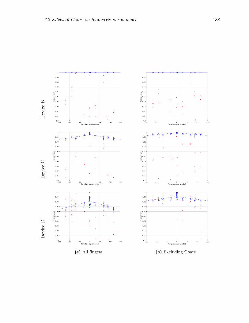
7.3 E�ect of Goats on biometric permanence 138
DeviceB
DeviceC
DeviceD
(a) All �ngers (b) Excluding Goats
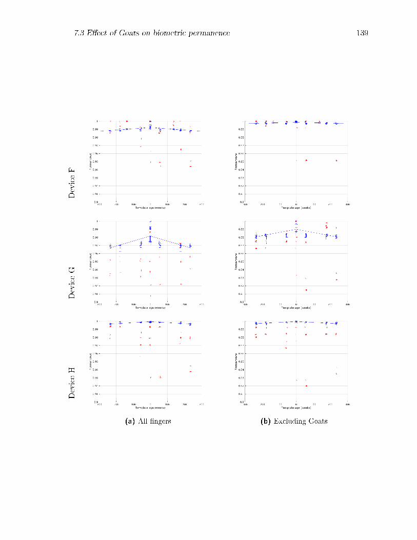
7.3 E�ect of Goats on biometric permanence 139
DeviceF
DeviceG
DeviceH
(a) All �ngers (b) Excluding Goats
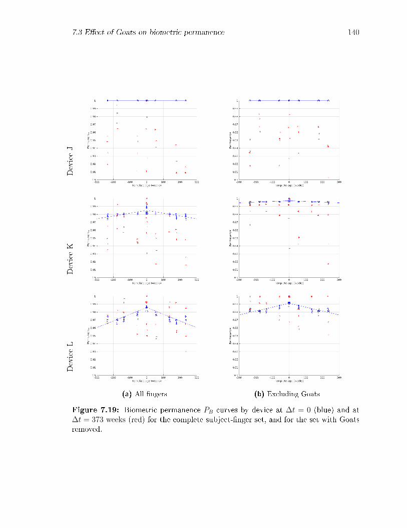
7.3 E�ect of Goats on biometric permanence 140
DeviceJ
DeviceK
DeviceL
(a) All �ngers (b) Excluding Goats
Figure 7.19: Biometric permanence PB curves by device at ∆t = 0 (blue) and at∆t = 373 weeks (red) for the complete subject-�nger set, and for the set with Goatsremoved.
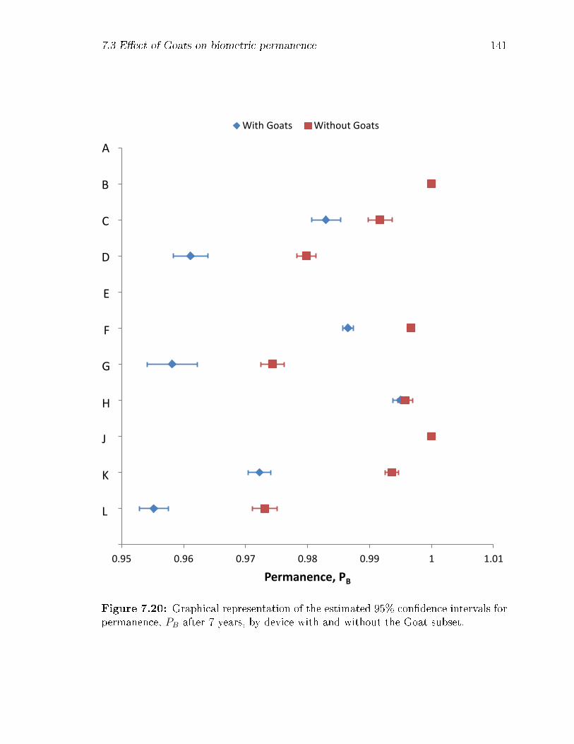
7.3 E�ect of Goats on biometric permanence 141
0
1
2
3
4
5
6
7
8
9
10
11
0.95 0.96 0.97 0.98 0.99 1 1.01
Permanence, PB
With Goats Without Goats
A
B
C
D
E
F
G
H
J
K
L
Figure 7.20: Graphical representation of the estimated 95% con�dence intervals forpermanence, PB after 7 years, by device with and without the Goat subset.
7.4 Discussion 142
7.4 Discussion
In this chapter, we applied a Doddington-like classi�cation scheme to the subject-
�ngers of the ISBIT/Norwood �ngerprint database, and were able to identify sets of
Goats, Lambs, and Wolves. We observed that these sets are substantially common
across the available �ngerprint capture devices so that, suggesting that they re�ect
intrinsic properties of the underlying biometric rather than extrinsic capabilities of the
devices themselves. We examined the available demographics of these sets, and found
strong evidence that older individuals and females are over-represented in the Goat set
(the subject-�ngers that contribute disproportionately to the FNMR), while younger
individuals are over-represented in both the Lamb and Wolf sets (the subject-�ngers
whose cross-matches contribute disproportionately to the FMR). Weak evidence was
found for males being more common amongst Wolves.
We then applied the NIST NFIQ metrics to the sets, and found that while Goats
are, on average, identi�ed as having lower biometric quality than the cohort of subject-
�ngers as a whole, both Lambs and Wolves are identi�ed as having higher quality.
This may hint at a fundamental di�culty in assessing biometric quality in a one-
to-many context � that is, to be truly informative about an individual's identity, a
biometric should in some sense maximize the distance between individuals' biometric
records.
Finally we revisited the concept of biometric permanence and showed that as well
as having a disproportionate e�ect on the classi�cation performance in general, Goats
are a signi�cant factor in limiting biometric permanence. This last observation may
have implications for the management of long-term IDMSs such as biometric pass-
ports, for example suggesting increasingly frequent re-enrolments of older individuals
in order to maintain overall IDMS performance.
Chapter 8
Discussion
8.1 Estimation of biometric permanence
In this work we have con�rmed the existence of biometric template ageing in a multi-
year, multi-vendor �ngerprint dataset obtained under perhaps more controlled condi-
tions (as detailed in Chapter 3) than those used in previous studies. The methodology,
outlined in Chapter 4, provides �rst-order elimination of systematic confounding fac-
tors in the study, at the expense of imposing an assumption about the time-symmetry
of the ageing e�ect. The amount of ageing observed was somewhat vendor-dependent,
and consistent with the baseline performance of the devices, i.e. those with better
than average classi�cation performance at time t = 0 display a slower decrease in
permanence (Chapter 5).
8.1.1 Motivation for the biometric permanence metric
Previous studies of biometric template ageing have reported their results in terms of
change in genuine match score [13] and/or the change in a single measure of classi-
�cation accuracy such as true match rate (TMR) [86]. From an operational point of
view however, it is important to consider both security (via FMR or TNMR) and con-
143
8.1 Estimation of biometric permanence 144
venience (via FNMR or TMR). Uludag et al. for example used changes in the equal
error rate (EER) [77]: this measure e�ectively gives equal weight to both factors. In
contrast, our proposed de�nition of biometric permanence, PB (Equation 4.1) empha-
sizes operational security by considering the change in FNMR (convenience) at �xed
FMR (security). Furthermore, by normalizing the metric to the time-zero FNMR, we
obtain a metric that permits comparisons across biometric systems of varying baseline
performance. Some other desirable properties are outlined in Section 4.2.1.
8.1.2 Assumptions and limitations
Although the results we obtained in Chapter 5 seem intuitively reasonable, we were
not able to provide an independent evaluation of biometric permanence by way of
comparison with our results.
As already noted, a key assumption of the forward-backward �matched delta�
methodology is that the change in match score is time-symmetric. The validity of
this assumption will depend on how the match scores are evaluated: in Section 5.3.1
we posited a case in which it might be violated. The method also assumes that
the confounding e�ect of gross visit-to-visit variability can be expressed (at least to
leading order) in the form of additive bias terms.
We can imagine a �thought experiment� to explore the validity of these assump-
tions (and that of the underlying model, Equation 4.3). In such an experiment one
would perform an ensemble of many studies, taking a ��x � block � randomize� ap-
proach to the ensemble design. For example:
� always employ the same test administrator(s) [FIX]
� conduct the data collections under the same environmental conditions (time of
year, location, humidity) [FIX] or conduct multiple collections and subdivide
the analyses by condition [BLOCK]

8.1 Estimation of biometric permanence 145
� conduct many studies over a variety of ambient conditions and test personnel
and aggregate them in a meta-analysis [RANDOMIZE]
If the assumptions of the matched-delta model are valid, then the results naïve ap-
plication of Equation 4.1 across the ensemble should converge to those of the matched
delta method. In 4.3.2 we in fact simulated such an ensemble, randomizing the visit
biases am, bn. In principle, one could do the same with real data however the scale of
such an experiment is beyond the scope of the present study.
In the simulated results of Chapter 4, it was also assumed that the imposter
distributions were constant over time. Subsequent analysis of the experimental data
cast doubt on this assumption, at least in the case of some devices in the study, and
in Chapter 5 we removed this restriction (Section 5.3.2).
8.1.3 Illustrative application of the metric
To illustrate the potential application of the biometric permanence methodology and
results, consider a biometric system based on our Device K. From Table 5.1, we
estimated its permanence after 7 years as PB = 97.2 ± 0.19. Suppose the system
is designed to operate at a FMR of 1 % and that the corresponding FNMR upon
commissioning the system is found to be 1.5 %: then, using Equation 4.1, we can
estimate the attainable FNMR after 7 years if the FMR is to be maintained as
FNMR∆t = 1− PB (1− FNMR0) = 1− (0.972)(0.985) = 0.043
i.e. the FNMR can be expected to degrade from 1.5 % to approximately 4 % over this
time period.
Even taking into account the ±0.19 uncertainty, this value is somewhat larger
than that which might be inferred from the DET curve of Figure 5.10b - suggesting
that the simple extrapolation overestimates the slope of PB.
8.2 Validation of NFIQ quality metrics 146
8.2 Validation of NFIQ quality metrics
Next, we applied the NIST NFIQ quality metrics on our labelled data, con�rming
the predictive capability of these metrics with respect to �ngerprint classi�cation
accuracy � e�ectively using our study as an independent validation dataset for NFIQ.
We observed essentially equivalent error-rate versus reject ratio from the two available
implementations, NFIQ-1 and NFIQ-2, noting that NFIQ-2 is nevertheless preferred
from an operational point of view because of its �ner-grained scale (Chapter 6).
Results for NFIQ were compared with those for vendor-provided quality values, where
available.
The novelty of these results really comes from the data rather than from any
methodological considerations. Data used in the training and validation of the NFIQ
classi�ers is dominated by US Government datasets (in the case of NFIQ-1, these were
DOS-C, DHS2-C, DHS10, TXDPS, and BEN for training alone, with the addition of
VISIT_POE and VISIT_POE_BVA for validation [74]), which might be assumed to
share certain common characteristics of acquisition and processing. In contrast, the
speci�cations and data acquisition protocols for our study were developed on behalf
of the ILO, with an initial focus on vendor interoperability: it is interesting to explore
how well the NFIQ measures perform on an independent dataset such as this.
8.3 Presence of a biometric menagerie
Subject-dependence of the classi�cation performance was also explored, based on a
modi�ed version of the criteria originally proposed by Doddington. A relatively small
subset of `Goat'-like subject-�ngers was identi�ed, and con�rmed to be substantially
vendor-independent, suggesting that such �ngers (which match poorly against them-
selves, and hence dominate the FNMR) are intrinsic, rather than a result of speci�c
image capture technologies or feature extraction algorithms. Dependencies on the
8.4 Biometrics as a communication channel 147
available demographic factors were evaluated, with signi�cant e�ects being found for
subject sex and for chronological age at time of enrolment (or Birth Year). `Lamb'
and `Wolf' subsets (which match too well against one another, together contributing
disproportionately to the FMR) were also identi�ed and examined: although repre-
senting a small fraction of the available imposter matches, these subsets substantially
cover the set of subject-�ngers as a whole, and their demographics are, unsurprisingly,
not signi�cantly di�erent from it in most cases. The one exception was Birth Year,
with both Lambs and Wolves appearing to favour younger individuals. It might be
instructive to repeat this analysis with a more exclusive de�nition of the `Lamb' and
`Wolf' subsets: they are large because of the choice of target FMR, which in turn was
driven by a desire to operate each of the devices somewhere in the �knee� region of
its DET curve.
Finally we examined the e�ect of subject-dependence on template ageing be-
haviour, and demonstrated (by removing them from the dataset) the importance
of Goats in the magnitude of the observed ageing.
In the following sections, we consider the information-theoretic interpretation of
template ageing, and its relation to biometric quality.
8.4 Biometrics as a communication channel
An information-theoretic model of a communications channel may be constructed as
follows (see for example Cover and Thomas §7.5 [8]).
A messageW is drawn from an index set {1, 2 . . .M}. We transmit a signalXn(W )
which is a sequence of n symbols from the alphabet of some random variable X. A
receiver receives signal Y n related to transmitted signal Xn by a channel transition
matrix p(yn|xn). The task of the receiver is to infer W from Y n using some decision
rule W = g(Y n).

8.4 Biometrics as a communication channel 148
We can imagine a similar formalism for a biometric system. That is, an individual
W is drawn from an an index set {1, 2 . . .M} of enrolled subjects. Associated with
W is a biometric record Xn(W ) which is a collection (or vector) of features, such
as a list of �ngerprint minutiae. A veri�er observes a biometric Y n related to the
record Xn by a biometric transition matrix p(yn|xn), and the task of the veri�er
is to infer the identity W from the observed biometric Y n using some decision rule
W = g(Y n) - or, in the case of a biometric veri�cation system, to estimate the
probability P (W = w|Y n) for some claimed identity w.
8.4.1 Biometric rate and capacity
In this formalism, we see that a biometric modality becomes a channel for the trans-
mission of information about an individual's identity. We may then ask about the
characteristics of this channel. For example, we might model the disappearance or
obfuscation of individual �ngerprint minutiae, perhaps as the result of occupational
damage, as erasures in an erasure channel; or the uncertainties in minutia location as
positional noise in a manner similar to that in an AWGN channel1. We might also
be able to talk about the rate of a biometric system in terms of the cardinality of the
subject set and the size of the biometric record:
R =log2M
n(8.1)
Given this de�nition of biometric rate, it might then be possible to de�ne a bio-
metric capacity C for a modality as the supremum of all achievable rates for the
channel: in principle, this would allow us to compare the fundamental e�ciency of
di�erent modalities, and to compare implementations within a modality based on
how closely their rate approaches C.
1For a discussion of these and other standard channel models, see for example Cover and Thomas(op. cit.) §7.1.
8.5 Information-theoretic interpretation of template ageing 149
Probably the biometric modality whose information-theoretic foundation has been
developed most explicitly is that of Daugman's IrisCodes [14], whose templates take
the form of binary sequences whose match scores are evaluated in terms of Ham-
ming distance [15]. In particular, by developing a hidden Markov model (HMM) for
IrisCode generation and tuning its parameters to obtain a best match to the observed
FMR of real irises, Daugman et al. were able to obtain an estimate for the capacity
of the IrisCode channel as 0.469 bits/bit [16]. A white noise analysis of the encoding
procedure estimated a theoretical maximum capacity of 0.566 bits/bit: the di�erence
being attributed to correlation between regions of the real iris.
8.4.2 Biometric �good codes�
Of course, much e�ort is directed in the �eld of communications towards the design of
good (high rate) channel codes: that is, sets of codewords Xn for which R approaches
C. In the case of linear block codes for example, one may imagine an (n, k) code as
mapping a k-bit message space into a n-bit codeword space; good codes essentially
maximize the minimum distance between codewords, making it easier to place a set
of decision boundaries between them at the receiver. In the biometric analogue,
codewords are biometric templates and clearly we do not have the same freedom to
choose them: we do however have at least some ability to include more informative
(and exclude less informative) features. Conceptually, this is similar to how the NFIQ
quality metrics attempt to identify high quality �ngerprints.
8.5 Information-theoretic interpretation of template age-
ing
When applied to the problem of biometric template ageing, the information-theoretic
approach implies that what we are observing is a decrease in mutual information, over
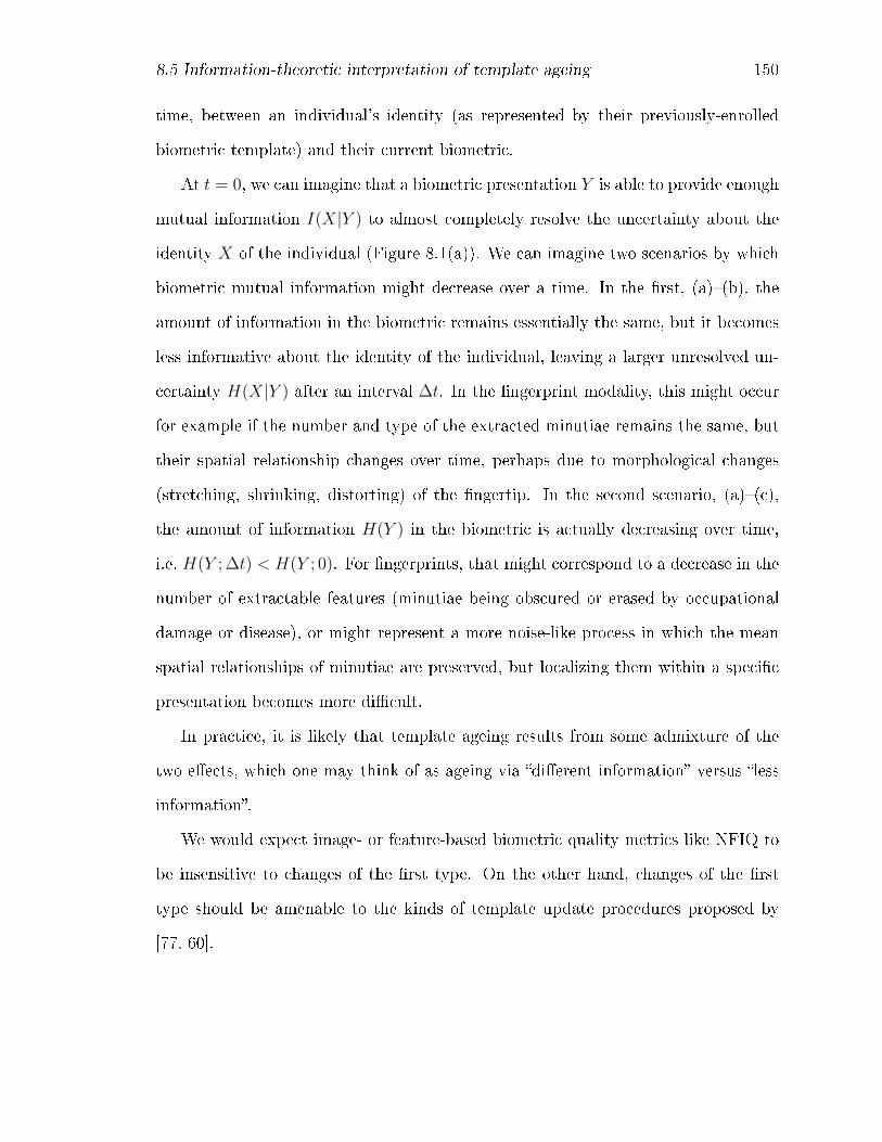
8.5 Information-theoretic interpretation of template ageing 150
time, between an individual's identity (as represented by their previously-enrolled
biometric template) and their current biometric.
At t = 0, we can imagine that a biometric presentation Y is able to provide enough
mutual information I(X|Y ) to almost completely resolve the uncertainty about the
identity X of the individual (Figure 8.1(a)). We can imagine two scenarios by which
biometric mutual information might decrease over a time. In the �rst, (a)�(b), the
amount of information in the biometric remains essentially the same, but it becomes
less informative about the identity of the individual, leaving a larger unresolved un-
certainty H(X|Y ) after an interval ∆t. In the �ngerprint modality, this might occur
for example if the number and type of the extracted minutiae remains the same, but
their spatial relationship changes over time, perhaps due to morphological changes
(stretching, shrinking, distorting) of the �ngertip. In the second scenario, (a)�(c),
the amount of information H(Y ) in the biometric is actually decreasing over time,
i.e. H(Y ; ∆t) < H(Y ; 0). For �ngerprints, that might correspond to a decrease in the
number of extractable features (minutiae being obscured or erased by occupational
damage or disease), or might represent a more noise-like process in which the mean
spatial relationships of minutiae are preserved, but localizing them within a speci�c
presentation becomes more di�cult.
In practice, it is likely that template ageing results from some admixture of the
two e�ects, which one may think of as ageing via �di�erent information� versus �less
information�.
We would expect image- or feature-based biometric quality metrics like NFIQ to
be insensitive to changes of the �rst type. On the other hand, changes of the �rst
type should be amenable to the kinds of template update procedures proposed by
[77, 60].
8.5 Information-theoretic interpretation of template ageing 151
𝐼 𝑋; 𝑌
𝐻 𝑋 𝑌 𝐼 𝑋; 𝑌 𝐻 𝑋 𝑌 𝐼 𝑋; 𝑌
𝐻(𝑋) 𝐻(𝑌; 0)
𝐻(𝑋) 𝐻(𝑌; ∆𝑡) 𝐻(𝑋) 𝐻(𝑌; ∆𝑡)
(a)
(b) (c) Figure 8.1: Conceptual scenarios for a decrease in biometric mutual information overtime. At time zero (a), almost all of the uncertainty H(X) about the individual'sidentity X is resolved by knowing the biometric Y . In (b), the amount of informationH(Y ; ∆t) provided by the biometric after time interval ∆t is the same, but less of itis helpful in determining the individual's identity. In (c), the biometric after interval∆t is intrinsically less informative, H(Y ; ∆t) < H(Y ; 0).

8.6 Suggestions for future work 152
8.6 Suggestions for future work
We have deduced that, at least conceptually, there are two mechanisms for the changes
in biometric match score over time. �Ageing via less information� would be asymmet-
ric, and represents (or at least, will be indistinguishable from) chronological ageing
of the individual. �Ageing via di�erent information� on the other hand is symmetric.
In the case of genuine matches, it is easy to see how both e�ects might con-
tribute to decreased match scores over time (i.e. to increased FNMR). The behaviour
with respect to imposter matches is less obvious, and may depend on how exactly
the particular scoring algorithm evaluates biometric similarity. For example, do two
presentations that have low information content (few extractable minutiae), but are
nevertheless similar, score higher or lower than two others that have many extractable
minutiae but di�er with respect to a few of them? Indeed, we saw evidence in Chap-
ter 5 that changes in imposter score distributions for many devices were negligible -
but not for all.
The measure of template ageing, PB (biometric permanence) used in the present
work was de�ned in terms of reduction in FNMR at �xed FMR, and re�ects changes in
both genuine and imposter match scores - the latter implicitly, by allowing the binary
decision threshold to vary in order to maintain the chosen FMR. In future work,
it might be instructive to maintain a constant threshold, and attempt to evaluate
changes in FNMR and FMR separately. Alternatively, one might consider using
variation of the decision threshold for constant FMR to be a proxy for changes in the
imposter distributions.
The biometric menagerie classi�cations of Chapter 7 turned out to have a richer
demographic structure than anticipated, and it would be worthwhile to revisit a num-
ber of aspects. In particular, the canonical categories of Sheep, Goats, Lambs and
Wolves are rather broad, being based either on FNMR or FMR: a more re�ned cate-
gorization such as the one proposed by Yager & Dunstone [84] may yield additional

8.6 Suggestions for future work 153
insight into the interplay of genuine and imposter match scores. At least, the demo-
graphic analysis of Lambs and Wolves might be enhanced by tightening the thresholds
for inclusion into those subsets, reducing their size and so potentially making them
more distinct from the cohort as a whole.
Finally, although the proposed permanence measure PB and the methodology de-
veloped for evaluating it have shown promising results when applied to our moderately
large �ngerprint dataset, it will be important to evaluate them much more widely -
preferably with even larger datasets and over additional biometric modalities.

Appendix A
Sample MSSQL database queries
Listing A.1: Simple query, for the author's own demographic and visit information1 USE Norwood
2
3 SELECT * FROM Subject WHERE Id = 256
4
5 SELECT AlgorithmOrderEnrol , AlgorithmOrderVerify , EnrolBeganOn , VerifyEndedOn
6 FROM dbo.Subject_Visit_Map
7 WHERE SubjectId = 256
Listing A.2: A complicated query, for biometric qualities of match transactions withgenuine/imposter class labelling
1 USE Norwood
2
3 SELECT eo.AlgorithmId , eo.VisitId , eo.SubjectId , nfiqA.FingerPosition , nfiqA.
IsSecondary ,
4 CASE WHEN nfiqA.FingerPosition = evq.FingerSecondary THEN evq.SecondaryQuality ELSE
evq.PrimaryQuality END AS [VendorQ],
5 (SELECT MIN(v) FROM (VALUES (nfiqA.Score), (nfiqB.Score), (nfiqC.Score)) AS value(v))
AS [NFIQ(min)],
6 (SELECT AVG(v) FROM (VALUES (nfiqA.Score), (nfiqB.Score), (nfiqC.Score)) AS value(v))
AS [NFIQ(avg)],
7 (SELECT MAX(v) FROM (VALUES (nfiqA.Score), (nfiqB.Score), (nfiqC.Score)) AS value(v))
AS [NFIQ(max)],
8 (SELECT MIN(v) FROM (VALUES (nfiq2A.Score), (nfiq2B.Score), (nfiq2C.Score)) AS value(
v)) AS [NFIQ2(min)],
9 (SELECT AVG(v) FROM (VALUES (nfiq2A.Score), (nfiq2B.Score), (nfiq2C.Score)) AS value(
v)) AS [NFIQ2(avg)],
10 (SELECT MAX(v) FROM (VALUES (nfiq2A.Score), (nfiq2B.Score), (nfiq2C.Score)) AS value(
v)) AS [NFIQ2(max)],
11 -- see https :// stackoverflow.com/a/6871572/4440445 "SQL MAX of multiple columns ?"
12 vo.SubjectId , vo.FingerPosition , vo.Attempt , vi.Presentation , mp.Score ,
13 CASE WHEN vo.SubjectId = eo.SubjectId AND vo.FingerPosition IN (et.FingerPrimary , et.
FingerSecondary) THEN 1 ELSE 0 END AS [GEN]
14 FROM
15 dbo.EnrolTemplate et INNER JOIN dbo.EnrolOnline eo ON eo.Id = et.EnrolOnlineId
16 INNER JOIN dbo.EnrolVendorQuality evq ON evq.EnrolOnlineId = eo.Id
17 INNER JOIN dbo.EnrolNFIQ nfiqA ON nfiqA.EnrolOnlineId = eo.Id
18 INNER JOIN dbo.EnrolNFIQ nfiqB ON nfiqB.EnrolOnlineId = eo.Id AND nfiqB.
FingerPosition = nfiqA.FingerPosition
19 INNER JOIN dbo.EnrolNFIQ nfiqC ON nfiqC.EnrolOnlineId = eo.Id AND nfiqC.
FingerPosition = nfiqA.FingerPosition
20 INNER JOIN dbo.EnrolNFIQ2 nfiq2A ON nfiq2A.EnrolOnlineId = eo.Id AND nfiq2A.
FingerPosition = nfiqA.FingerPosition
21 INNER JOIN dbo.EnrolNFIQ2 nfiq2B ON nfiq2B.EnrolOnlineId = eo.Id AND nfiq2B.
FingerPosition = nfiq2A.FingerPosition
154
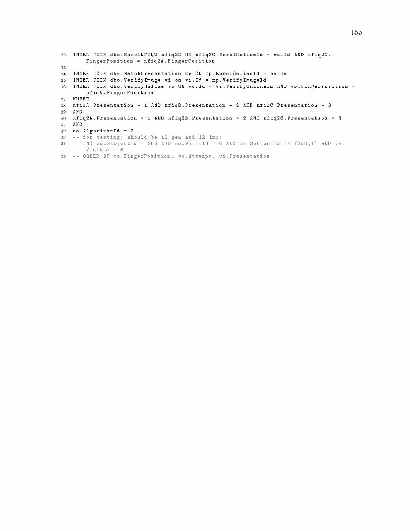
155
22 INNER JOIN dbo.EnrolNFIQ2 nfiq2C ON nfiq2C.EnrolOnlineId = eo.Id AND nfiq2C.
FingerPosition = nfiq2A.FingerPosition
23
24 INNER JOIN dbo.MatchPresentation mp ON mp.EnrolOnlineId = eo.Id
25 INNER JOIN dbo.VerifyImage vi on vi.Id = mp.VerifyImageId
26 INNER JOIN dbo.VerifyOnline vo ON vo.Id = vi.VerifyOnlineId AND vo.FingerPosition =
nfiqA.FingerPosition
27 WHERE
28 nfiqA.Presentation = 1 AND nfiqB.Presentation = 2 AND nfiqC.Presentation = 3
29 AND
30 nfiq2A.Presentation = 1 AND nfiq2B.Presentation = 2 AND nfiq2C.Presentation = 3
31 AND
32 eo.AlgorithmId = 2
33 -- for testing; should be 12 gen and 12 imp:
34 -- AND eo.SubjectId = 256 AND eo.VisitId = 6 AND vo.SubjectId IN (256 ,1) AND vo.
VisitId = 6
35 -- ORDER BY vo.FingerPosition , vo.Attempt , vi.Presentation
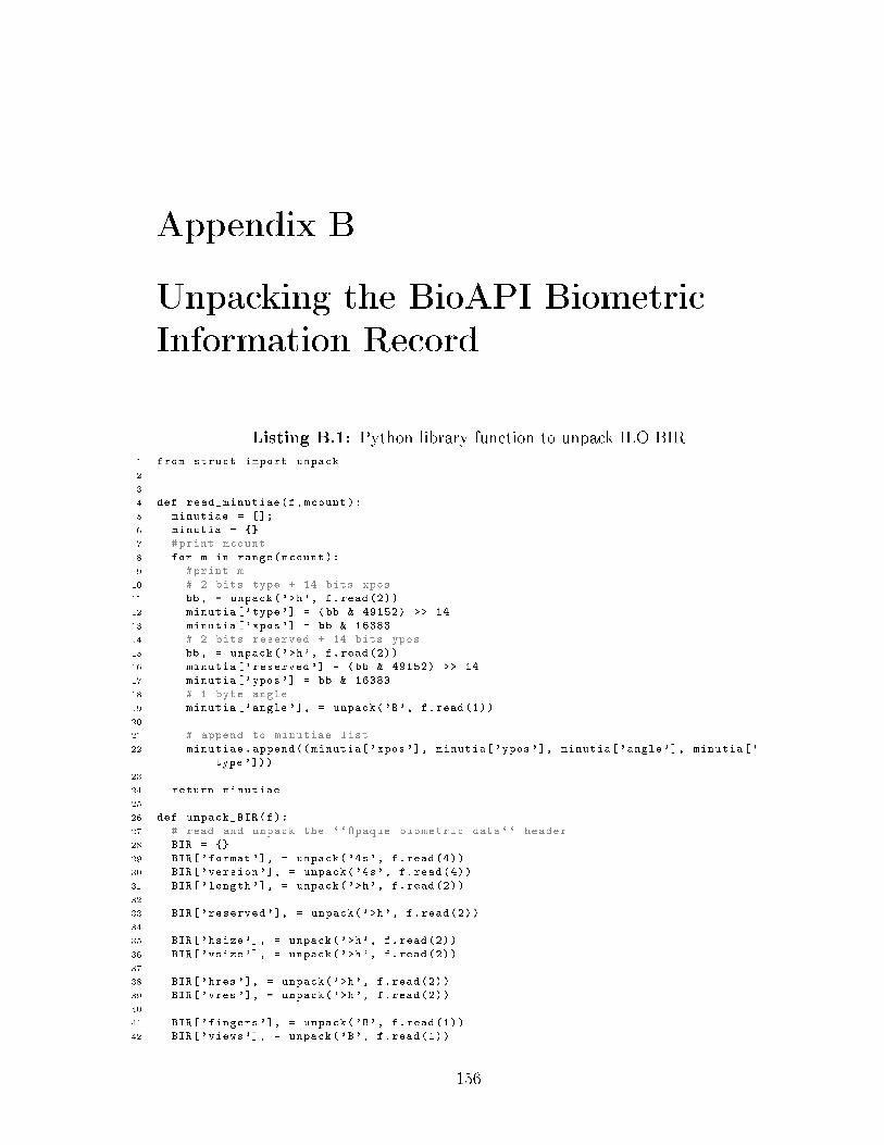
Appendix B
Unpacking the BioAPI BiometricInformation Record
Listing B.1: Python library function to unpack ILO BIR1 from struct import unpack
2
3
4 def read_minutiae(f,mcount):
5 minutiae = [];
6 minutia = {}
7 #print mcount
8 for m in range(mcount):
9 #print m
10 # 2 bits type + 14 bits xpos
11 bb, = unpack('>h', f.read (2))
12 minutia['type'] = (bb & 49152) >> 14
13 minutia['xpos'] = bb & 16383
14 # 2 bits reserved + 14 bits ypos
15 bb, = unpack('>h', f.read (2))
16 minutia['reserved '] = (bb & 49152) >> 14
17 minutia['ypos'] = bb & 16383
18 # 1 byte angle
19 minutia['angle'], = unpack('B', f.read (1))
20
21 # append to minutiae list
22 minutiae.append (( minutia['xpos'], minutia['ypos'], minutia['angle '], minutia['
type']))
23
24 return minutiae
25
26 def unpack_BIR(f):
27 # read and unpack the ``Opaque biometric data `` header
28 BIR = {}
29 BIR['format '], = unpack('4s', f.read (4))
30 BIR['version '], = unpack('4s', f.read (4))
31 BIR['length '], = unpack('>h', f.read (2))
32
33 BIR['reserved '], = unpack('>h', f.read (2))
34
35 BIR['hsize'], = unpack('>h', f.read (2))
36 BIR['vsize'], = unpack('>h', f.read (2))
37
38 BIR['hres'], = unpack('>h', f.read (2))
39 BIR['vres'], = unpack('>h', f.read (2))
40
41 BIR['fingers '], = unpack('B', f.read (1))
42 BIR['views'], = unpack('B', f.read (1))
156
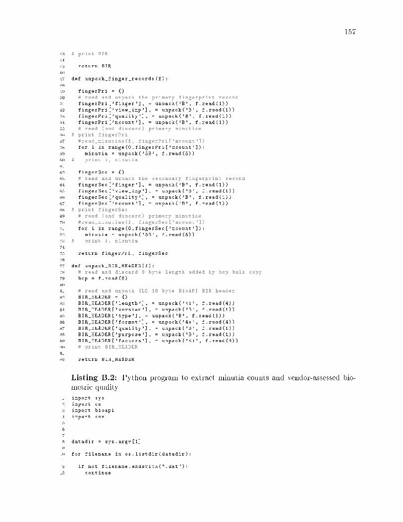
157
43 # print BIR
44
45 return BIR
46
47 def unpack_finger_records(f):
48
49 fingerPri = {}
50 # read and unpack the primary fingerprint record
51 fingerPri['finger '], = unpack('B', f.read (1))
52 fingerPri['view_imp '], = unpack('B', f.read (1))
53 fingerPri['quality '], = unpack('B', f.read (1))
54 fingerPri['mcount '], = unpack('B', f.read (1))
55 # read (and discard) primary minutiae
56 # print fingerPri
57 #read_minutiae(f, fingerPri['mcount '])
58 for i in range(0, fingerPri['mcount ']):
59 minutia = unpack('5B', f.read (5))
60 # print i, minutia
61
62 fingerSec = {}
63 # read and unpack the secondary fingerprint record
64 fingerSec['finger '], = unpack('B', f.read (1))
65 fingerSec['view_imp '], = unpack('B', f.read (1))
66 fingerSec['quality '], = unpack('B', f.read (1))
67 fingerSec['mcount '], = unpack('B', f.read (1))
68 # print fingerSec
69 # read (and discard) primary minutiae
70 #read_minutiae(f, fingerSec['mcount '])
71 for i in range(0, fingerSec['mcount ']):
72 minutia = unpack('5B', f.read (5))
73 # print i, minutia
74
75 return fingerPri , fingerSec
76
77 def unpack_BIR_HEADER(f):
78 # read and discard 8 byte length added by bcp bulk copy
79 bcp = f.read (8)
80
81 # read and unpack ILO 16 byte BioAPI BIR header
82 BIR_HEADER = {}
83 BIR_HEADER['length '], = unpack('<i', f.read (4))
84 BIR_HEADER['version '], = unpack('B', f.read (1))
85 BIR_HEADER['type'], = unpack('B', f.read (1))
86 BIR_HEADER['format '], = unpack('4s', f.read (4))
87 BIR_HEADER['quality '], = unpack('B', f.read (1))
88 BIR_HEADER['purpose '], = unpack('B', f.read (1))
89 BIR_HEADER['factors '], = unpack('<i', f.read (4))
90 # print BIR_HEADER
91
92 return BIR_HEADER
Listing B.2: Python program to extract minutia counts and vendor-assessed bio-metric quality
1 import sys
2 import os
3 import bioapi
4 import csv
5
6
7
8 datadir = sys.argv [1]
9
10 for filename in os.listdir(datadir):
11
12 if not filename.endswith(".dat"):
13 continue
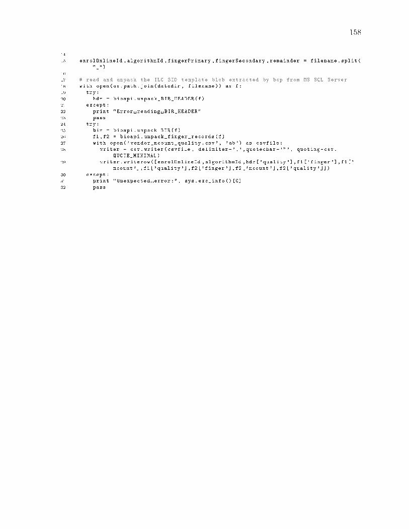
158
14
15 enrolOnlineId ,algorithmId ,fingerPrimary ,fingerSecondary ,remainder = filename.split(
"_")
16
17 # read and unpack the ILO SID template blob extracted by bcp from MS SQL Server
18 with open(os.path.join(datadir , filename)) as f:
19 try:
20 hdr = bioapi.unpack_BIR_HEADER(f)
21 except:
22 print "Error reading BIR_HEADER"
23 pass
24 try:
25 bir = bioapi.unpack_BIR(f)
26 f1,f2 = bioapi.unpack_finger_records(f)
27 with open('vendor_mcount_quality.csv', 'ab') as csvfile:
28 writer = csv.writer(csvfile , delimiter=',',quotechar='"', quoting=csv.
QUOTE_MINIMAL)
29 writer.writerow ([ enrolOnlineId ,algorithmId ,hdr['quality '],f1['finger '],f1['
mcount '],f1['quality '],f2['finger '],f2['mcount '],f2['quality ']])
30 except:
31 print "Unexpected error:", sys.exc_info ()[0]
32 pass
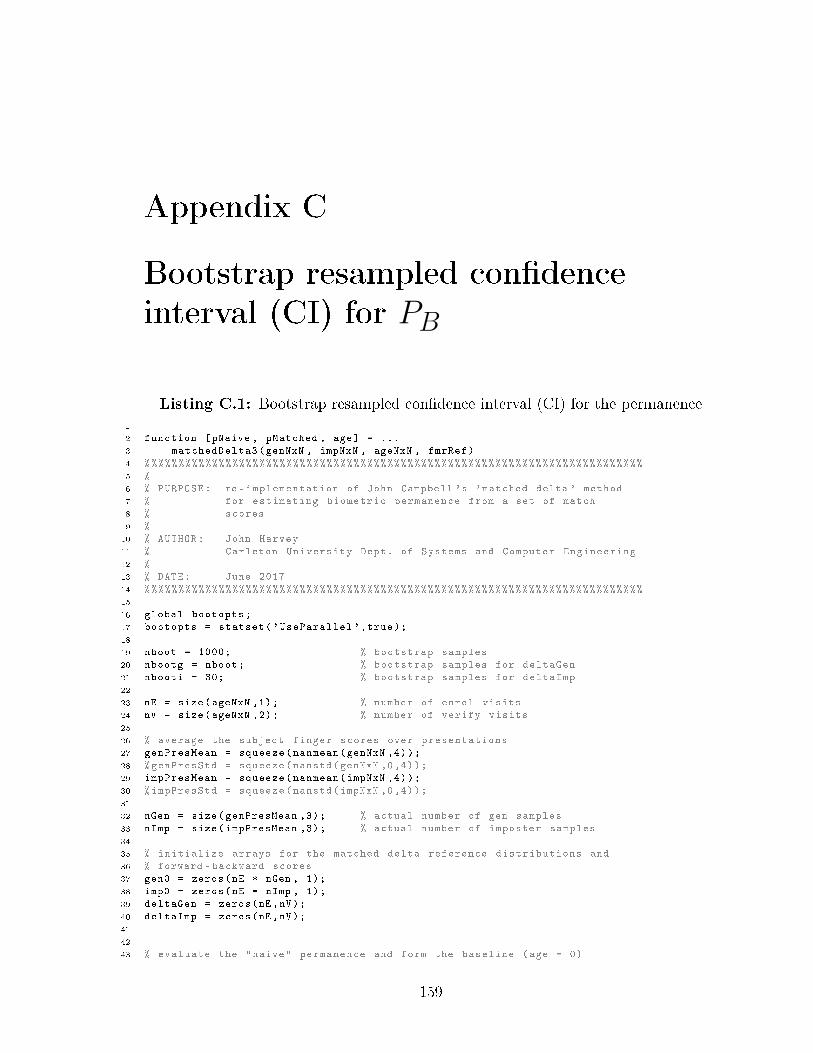
Appendix C
Bootstrap resampled con�denceinterval (CI) for PB
Listing C.1: Bootstrap resampled con�dence interval (CI) for the permanence1
2 function [pNaive , pMatched , age] = ...
3 matchedDelta3(genNxN , impNxN , ageNxN , fmrRef)
4 %%%%%%%%%%%%%%%%%%%%%%%%%%%%%%%%%%%%%%%%%%%%%%%%%%%%%%%%%%%%%%%%%%%%%%%%%%
5 %
6 % PURPOSE: re-implementation of John Campbell 's 'matched delta ' method
7 % for estimating biometric permanence from a set of match
8 % scores
9 %
10 % AUTHOR: John Harvey
11 % Carleton University Dept. of Systems and Computer Engineering
12 %
13 % DATE: June 2017
14 %%%%%%%%%%%%%%%%%%%%%%%%%%%%%%%%%%%%%%%%%%%%%%%%%%%%%%%%%%%%%%%%%%%%%%%%%%
15
16 global bootopts;
17 bootopts = statset('UseParallel ',true);
18
19 nboot = 1000; % bootstrap samples
20 nbootg = nboot; % bootstrap samples for deltaGen
21 nbooti = 30; % bootstrap samples for deltaImp
22
23 nE = size(ageNxN ,1); % number of enrol visits
24 nV = size(ageNxN ,2); % number of verify visits
25
26 % average the subject -finger scores over presentations
27 genPresMean = squeeze(nanmean(genNxN ,4));
28 %genPresStd = squeeze(nanstd(genNxN ,0,4));
29 impPresMean = squeeze(nanmean(impNxN ,4));
30 %impPresStd = squeeze(nanstd(impNxN ,0,4));
31
32 nGen = size(genPresMean ,3); % actual number of gen samples
33 nImp = size(impPresMean ,3); % actual number of imposter samples
34
35 % initialize arrays for the matched delta reference distributions and
36 % forward -backward scores
37 gen0 = zeros(nE * nGen , 1);
38 imp0 = zeros(nE * nImp , 1);
39 deltaGen = zeros(nE ,nV);
40 deltaImp = zeros(nE ,nV);
41
42
43 % evaluate the "naive" permanence and form the baseline (age = 0)
159

160
44 % aggregate distributions and matched deltas
45 pNaive = ones(nE, nV);
46 for i = 1:nE
47
48 tmr0 = tmrAtfmr(squeeze(genPresMean(i,i,:)), squeeze(impPresMean(i,i,:)), fmrRef ,
nboot);
49
50 % aggregate the baseline "zero time" distributions
51 gen0((i-1)*nGen +1:i*nGen) = genPresMean(i,i,:);
52 imp0((i-1)*nImp +1:i*nImp) = impPresMean(i,i,:);
53
54 for j = 1:nV
55 if (j ~= i)
56 tmr = tmrAtfmr(squeeze(genPresMean(i,j,:)), squeeze(impPresMean(i,j,:)),
fmrRef , nboot);
57 pNaive(i,j,:) = tmr/tmr0;
58 end
59
60 if (j > i) % (skip lower triangle because of symmetry)
61 % form the forward -backward matched deltas
62 deltaGen(i,j) = delta( genPresMean(i,j,:), genPresMean(j,i,:),
genPresMean(i,i,:), genPresMean(j,j,:), nbootg);
63 deltaImp(i,j) = delta( impPresMean(i,j,:), impPresMean(j,i,:),
impPresMean(i,i,:), impPresMean(j,j,:), nbooti);
64 end
65 end
66 end
67
68 % evaluate the matched deltas - note that we can use the symmetry to
69 % reduce the number of evaluations
70 inds = triu(ageNxN) ~= 0.;
71 PbCI = permMatchedDelta(gen0 , imp0 , deltaGen(inds)', deltaImp(inds)', fmrRef , nboot);
72 % short -circuit the acual evaluation (for quick testing of loops):
73 %PbCI = [ones(size(inds(inds))) ones(size(inds(inds))) ones(size(inds(inds)))]';
74
75 % flip and stitch to get a plottable permanence versus age
76 tmp = sortrows ([ ageNxN(inds)' ; PbCI]') ';
77 age = [-fliplr(tmp(1,:)) 0. tmp(1,:)];
78 pMatched = [fliplr(tmp (2:end ,:)) [1.;1.;1.] tmp (2:end ,:)];
79
80 end
81
82
83 function d = delta(sij , sji , sii , sjj , nboot)
84
85 % global bootopts;
86 %
87 % X = squeeze(sij) + squeeze(sji) - squeeze(sii) - squeeze(sjj);
88 %
89 % bootstat = bootstrp(nboot ,@nanmean ,X,'Options ',bootopts);
90 %
91 % d = 0.5 * mean(bootstat);
92
93 % JH 13-Jul -17: it doesn 't make sense to bootstrap the mean , since we know
94 % that the sample mean is a _sufficient statistic_ for the population mean
95 d = 0.5 * nanmean(sij + sji - sii - sjj);
96
97 end
98
99
100 function tmr = tmrAtfmr(gen , imp , fmrRef , nboot)
101
102 global bootopts;
103
104 nGen = size(gen ,1);
105 nImp = size(imp ,1);
106
107 % construct a single score vector and class labels
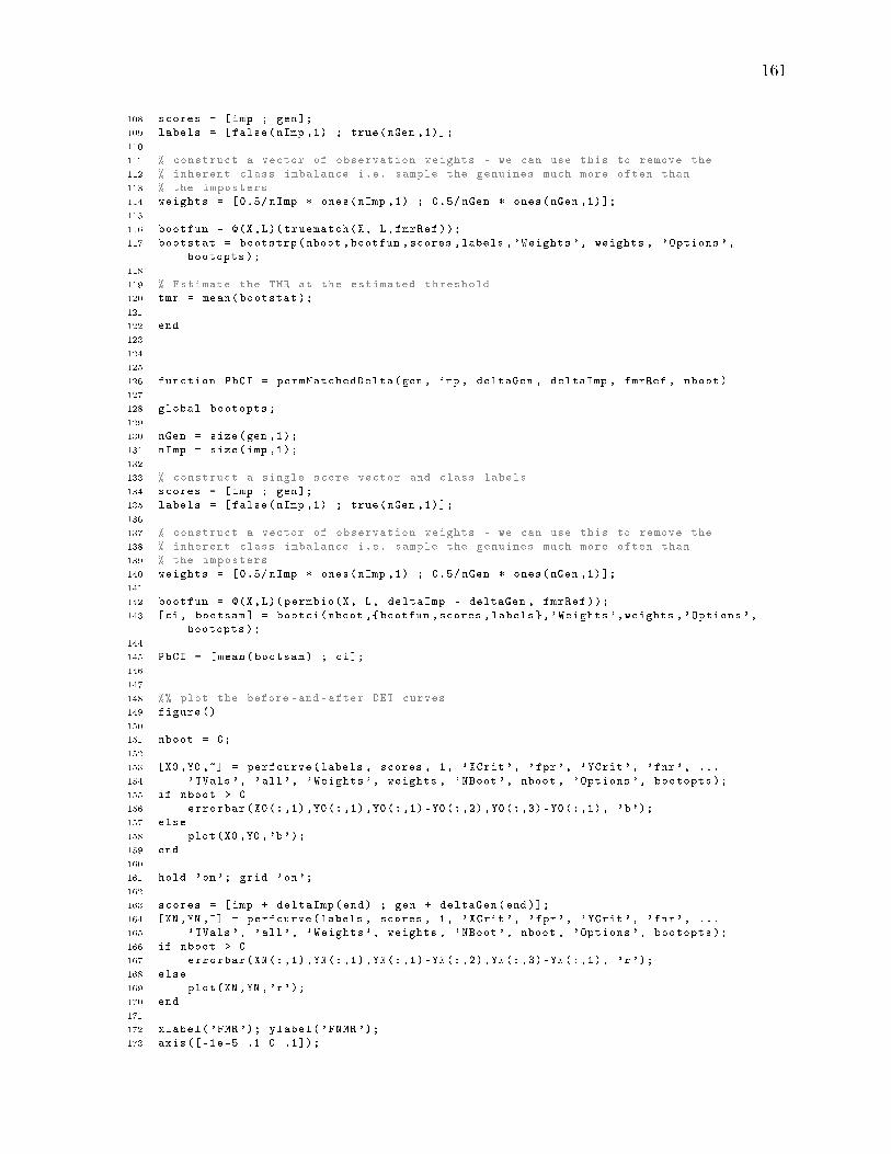
161
108 scores = [imp ; gen];
109 labels = [false(nImp ,1) ; true(nGen ,1)];
110
111 % construct a vector of observation weights - we can use this to remove the
112 % inherent class imbalance i.e. sample the genuines much more often than
113 % the imposters
114 weights = [0.5/ nImp * ones(nImp ,1) ; 0.5/ nGen * ones(nGen ,1)];
115
116 bootfun = @(X,L)(truematch(X, L,fmrRef));
117 bootstat = bootstrp(nboot ,bootfun ,scores ,labels ,'Weights ', weights , 'Options ',
bootopts);
118
119 % Estimate the TMR at the estimated threshold
120 tmr = mean(bootstat);
121
122 end
123
124
125
126 function PbCI = permMatchedDelta(gen , imp , deltaGen , deltaImp , fmrRef , nboot)
127
128 global bootopts;
129
130 nGen = size(gen ,1);
131 nImp = size(imp ,1);
132
133 % construct a single score vector and class labels
134 scores = [imp ; gen];
135 labels = [false(nImp ,1) ; true(nGen ,1)];
136
137 % construct a vector of observation weights - we can use this to remove the
138 % inherent class imbalance i.e. sample the genuines much more often than
139 % the imposters
140 weights = [0.5/ nImp * ones(nImp ,1) ; 0.5/ nGen * ones(nGen ,1)];
141
142 bootfun = @(X,L)(permbio(X, L, deltaImp - deltaGen , fmrRef));
143 [ci , bootsam] = bootci(nboot ,{bootfun ,scores ,labels},'Weights ',weights ,'Options ',
bootopts);
144
145 PbCI = [mean(bootsam) ; ci];
146
147
148 %% plot the before -and -after DET curves
149 figure ()
150
151 nboot = 0;
152
153 [X0 ,Y0 ,~] = perfcurve(labels , scores , 1, 'XCrit', 'fpr', 'YCrit', 'fnr', ...
154 'TVals', 'all', 'Weights ', weights , 'NBoot', nboot , 'Options ', bootopts);
155 if nboot > 0
156 errorbar(X0(:,1),Y0(:,1),Y0(:,1)-Y0(:,2),Y0(:,3)-Y0(:,1), 'b');
157 else
158 plot(X0,Y0,'b');
159 end
160
161 hold 'on'; grid 'on';
162
163 scores = [imp + deltaImp(end) ; gen + deltaGen(end)];
164 [XN ,YN ,~] = perfcurve(labels , scores , 1, 'XCrit', 'fpr', 'YCrit', 'fnr', ...
165 'TVals', 'all', 'Weights ', weights , 'NBoot', nboot , 'Options ', bootopts);
166 if nboot > 0
167 errorbar(XN(:,1),YN(:,1),YN(:,1)-YN(:,2),YN(:,3)-YN(:,1), 'r');
168 else
169 plot(XN,YN,'r');
170 end
171
172 xlabel('FMR'); ylabel('FNMR');
173 axis([-1e-5 .1 0 .1]);
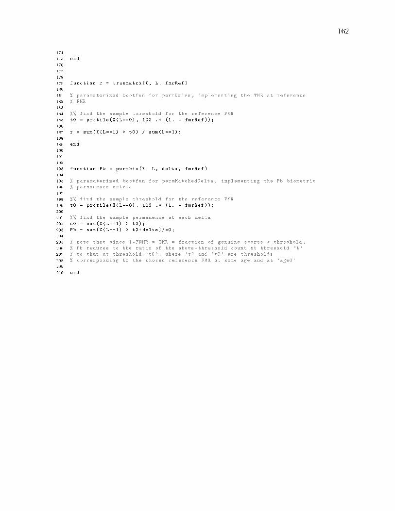
162
174
175 end
176
177
178
179 function r = truematch(X, L, fmrRef)
180
181 % paramaterized bootfun for permNaive , implementing the TMR at reference
182 % FMR
183
184 %% find the sample threshold for the reference FMR
185 t0 = prctile(X(L==0), 100 .* (1. - fmrRef));
186
187 r = sum(X(L==1) > t0) / sum(L==1);
188
189 end
190
191
192
193 function Pb = permbio(X, L, delta , fmrRef)
194
195 % paramaterized bootfun for permMatchedDelta , implementing the Pb biometric
196 % permanence metric
197
198 %% find the sample threshold for the reference FMR
199 t0 = prctile(X(L==0), 100 .* (1. - fmrRef));
200
201 %% find the sample permanence at each delta
202 c0 = sum(X(L==1) > t0);
203 Pb = sum(X(L==1) > t0+delta)/c0;
204
205 % note that since 1-FNMR = TMR = fraction of genuine scores > threshold ,
206 % Pb reduces to the ratio of the above -threshold count at threshold 't'
207 % to that at threshold 't0 ', where 't' and 't0' are thresholds
208 % corresponding to the chosen reference FMR at some age and at 'age0 '
209
210 end
Appendix D
A note on the Rayleigh synthetic
match score distributions
In Chapter 4, the choice was made to use Rayleigh distributions for the synthetic
genuine and imposter match scores. The initial justi�cation for this choice was sim-
ply that they �look about right�: for the imposter scores, we sought a well-known
distribution that had a hard cut-o� at a score of zero, with positive skew to represent
a long tail of high-scoring imposters (potential false matches). For the genuine scores,
a ��ipped� Rayleigh shape similarly provided a hard cut-o� maximum score � nor-
malized to one in our simulations � with a long tail of low-scoring genuines (potential
false non-matches).
No attempt was made to match the synthetic distributions to the actual score
distributions of the devices in our study. In fact, the actual distributions vary sig-
ni�cantly, re�ecting di�erences in the scoring algorithms between them (Figure 5.3 �
5.11).
One nice consequence of the choice of Rayleigh distributions is that the tail in-
tegrals (for the FMR and FNMR) in our classi�cation model remain obtainable in
closed form after the addition of noise, as will be shown in the following section. This
163
D.1 Tail integral for the FMR 164
provides some additional � albeit post-hoc � justi�cation for their choice.
D.1 Tail integral for the FMR
In the model of Section 4.2.2, a true biometric match score s is drawn from a genuine
(G) or imposter (I) score distribution, to which is added zero-mean Gaussian noise
W . The probability density function (pdf) of the sum of these random variables is
the convolution pW ∗ pI,G of their pdfs where
f ∗ g :=
∫ ∞
−∞f(x′)g(x− x′)dx′ (D.1)
For the pdf of the imposter scores, we have from Equation 4.5
pI(s) =s
β2I
e−s2/2β2I ; s ≥ 0 (D.2)
while the pdf of the noise may be written as
pW (s) =1√2πσ
e−s2/2σ2
(D.3)
so that the pdf of the sum becomes
pI+W (s) =1√2πσ
∫ ∞
0
s′
β2I
e−s′2/2β2I e−(s−s′)2/2σ2
ds′ (D.4)
The �trick� at this point is to realize that it is not necessary to evaluate this
convolution in closed form, in order to evaluate the tail integral. In particular, we
may write the resulting FMR as
PrI+W {s > θ} = PrW+I {s > θ} =
∫ ∞
θ
∫ ∞
−∞pW (s′)pI(s− s′)ds′ds (D.5)

D.1 Tail integral for the FMR 165
which, changing the order of integration, becomes
PrI+W {s > θ} =
∫ ∞
−∞pW (s′)
∫ ∞
θ
pI(s− s′)dsds′ (D.6)
in which the inner integral (with a further change of variables s− s′ → s) is now just
∫ ∞
θ
pI(s− s′)ds =
∫ ∞
θ−s′pI(s).ds (D.7)
which is just the probability that the noise-free imposter score is greater than θ− s′.
For the chosen Rayleigh distribution, this is easy to evaluate since
d
dse−s2/2β2
I = − s
β2I
e−s2/2β2I (D.8)
so that ∫ ∞
θ
pI(s− s′)ds =[e−s2/2β2
I
](θ−s′)
∞= e−(θ−s′)2/2β2
I (D.9)
Plugging this back into D.6, we have
PrI+W {s > θ} =1√2πσ
∫ ∞
θ
e−s′2/2σ2
e−(θ−s′)2/2β2Ids′ (D.10)
in which the integrand is just a product of two exponentials.1 From here on in, it is
just a matter of completing the square - that is,
s′2
2σ2+
(θ − s′)2
2β2I
=β2I s
′2 + σ2(θ − s′)2
2σ2β2I
(D.11)
=β2I + σ2
2σ2β2I
[s′2 − 2σ2θ
β2I + σ2
s′ +σ2θ2
β2I + σ2
](D.12)
=β2I + σ2
2σ2β2I
[(s′ − σ2θ
β2I + σ2
)2
+σ2θ2
β2I + σ2
− σ4θ2
β2I + σ2
](D.13)
1If we had preserved the original order, taking the inner integral over the noise distribution, theintegrand would have been the product of the Rayleigh distribution with an error function
D.2 Tail integral for the FNMR 166
giving
PrI+W {s > θ} =1√2πσ
e− θ2
2β2I
(1− σ2
β2I+σ2
) ∫ ∞
−∞e−β2I+σ2
2σ2β2I
(s′− σ2θ
β2I+σ2
)2
ds′ (D.14)
in which the standard de�nite integral may be evaluated from tables, yielding
PrI+W {s > θ} =
√β2I
β2I + σ2
e−θ2/2(β2I+σ2) (D.15)
By inspection, (D.15) implies that the noisy score remains Rayleigh distributed,
with parameter β2I → β2
I + σ2, i.e.
pI+W (s) =s
β2I + σ2
e−s2/2(β2I+σ2); s ≥ 0 (D.16)
D.2 Tail integral for the FNMR
Evaluation of the FNMR from the tail of the genuine distribution proceeds using allthe same steps as the previous section, but backwards and in heels.
Bibliography
[1] A. Adler, R. Youmaran, and S. Loyka. Towards a measure of biometric infor-mation. In 2006 Canadian Conference on Electrical and Computer Engineering,pages 210�213, 2006. doi: 10.1109/CCECE.2006.277447.
[2] P. N. Belhumeur, J. P. Hespanha, and D. J. Kriegman. Eigenfaces vs. �sherfaces:recognition using class speci�c linear projection. IEEE Trans. Pattern Anal.Mach. Intell., 19(7):711�720, July 1997. issn: 0162-8828. doi: 10.1109/34.598228.
[3] A. Bertillon. Signaletic Instructions Including the Theory and Practice of An-thropometrical Identi�cation. Werner Company, 1896.
[4] H. Bose. Hints on Finger-Prints, with a Telegraphic Code for Finger Impres-sions. Thacker, Spink and Company, Calcutta/Simla, 1917.
[5] M. E. Brockly. The Role of Test Administrator and Error. Master's thesis,Purdue University, West Lafayette, IN, 2013.
[6] C. Camden. Elizabethan chiromancy. Modern Language Notes, 62(1):1�7, 1947.issn: 01496611.
[7] L. Chen, J. Wang, S. Yang, and H. He. A �nger vein image-based personalidenti�cation system with self-adaptive illuminance control. IEEE Transactionson Instrumentation and Measurement, 66(2):294�304, 2017. issn: 0018-9456.doi: 10.1109/TIM.2016.2622860.
[8] T. M. Cover and J. A. Thomas. Channel capacity. In Elements of InformationTheory (Wiley Series in Telecommunications and Signal Processing). Wiley-Interscience, New York, NY, USA, 2006. Chapter 7. isbn: 0471241954.
[9] T. M. Cover and J. A. Thomas. Entropy, relative entropy, and mutual informa-tion. In Elements of Information Theory (Wiley Series in Telecommunicationsand Signal Processing). Wiley-Interscience, New York, NY, USA, 2006. Chap-ter 2. isbn: 0471241954.
[10] D. R. Cox. Biometrika: The �rst 100 years. Biometrika, 88(1):3�11, Feb. 2001.issn: 0006-3444. doi: 10.1093/biomet/88.1.3.
[11] N. J. Crane, E. G. Bartick, R. S. Perlman, and S. Hu�man. Infrared spectro-scopic imaging for noninvasive detection of latent �ngerprints. Journal of Foren-sic Sciences, 52(1):48�53, 2007. doi: 10.1111/j.1556-4029.2006.00330.x.
167
BIBLIOGRAPHY 168
[12] H. Cummins. Finger prints and attempted fraud. New Orleans Medical andSurgical Journal, 94:82�86, 1942.
[13] A. Czajka. In�uence of iris template aging on recognition reliability. In M.Fernández-Chimeno, P. L. Fernandes, S. Alvarez, D. Stacey, J. Solé-Casals, A.Fred, and H. Gamboa, editors, Biomedical Engineering Systems and Technolo-gies, pages 284�299, Berlin, Heidelberg. Springer Berlin Heidelberg, 2014. isbn:978-3-662-44485-6.
[14] J. Daugman. New methods in iris recognition. IEEE Transactions on Systems,Man, and Cybernetics, Part B (Cybernetics), 37(5):1167�1175, 2007. issn: 1083-4419. doi: 10.1109/TSMCB.2007.903540.
[15] J. Daugman. Probing the uniqueness and randomness of iriscodes: results from200 billion iris pair comparisons. Proceedings of the IEEE, 94(11):1927�1935,2006. issn: 0018-9219. doi: 10.1109/JPROC.2006.884092.
[16] J. Daugman. Information theory and the iriscode. IEEE Transactions on In-formation Forensics and Security, 11:400�409, 2016.
[17] G. Doddington, W. Liggett, A. Martin, M. Przybocki, and D. Reynolds. SHEEP,GOATS, LAMBS and WOLVES A statistical analysis of speaker performancein the nist 1998 speaker recognition evaluation. In International Conference onSpoken Language Processing, 1998.
[18] M. Drahansky, M. Dolezel, J. Urbanek, E. Brezinova, and T. Kim. In�uence ofskin diseases on �ngerprint recognition. Journal of Biomedicine and Biotech-nology, 2012. Article ID 626148.
[19] R. O. Duda, P. E. Hart, and D. G. Stork. Pattern Classi�cation (2nd Edition).Wiley-Interscience, New York, NY, USA, 2000. isbn: 0471056693.
[20] S. Elliott, E. Kukula, and N. Sickler. The challenges of the environment andthe human/biometric device. In Proc. International Workshop on BiometricTechnologies, 2004.
[21] D Exline, C Wallace, C. Roux, C. Lennard, N Nelson, and P Treado. Foren-sic applications of chemical imaging: latent �ngerprint detection using visibleabsorption and luminescence. English. Journal of forensic Science, 48(5):1047�1053, 2003. issn: 0022-1198.
[22] S. P. Fenker and K.W. Bowyer. Experimental evidence of a template aging e�ectin iris biometrics. In Proc. 2011 IEEE Workshop on Applications of ComputerVision (WACV) (WACV '11), pages 232�239, 2011.
[23] W. Freude, R. Schmogrow, B. Nebendahl, M. Winter, A. Josten, D. Hillerkuss,S. Koenig, J. Meyer, M. Dreschmann, M. Huebner, C. Koos, J. Becker, andJ. Leuthold. Quality metrics for optical signals: Eye diagram, Q-factor, OSNR,EVM and BER. In 2012 14th International Conference on Transparent OpticalNetworks (ICTON), pages 1�4, 2012. doi: 10.1109/ICTON.2012.6254380.

BIBLIOGRAPHY 169
[24] J. Galbally, S. Marcel, and J. Fierrez. Biometric antispoo�ng methods: a surveyin face recognition. IEEE Access, 2:1530�1552, 2014. issn: 2169-3536. doi: 10.1109/ACCESS.2014.2381273.
[25] F. Galton. Finger Prints. Macmillan and Co., London, 1892.
[26] P Grother, J. Matey, E Tabassi, G W. Quinn, and M Chumakov. IREX-VItemporal stability of iris recognition accuracy. NIST Interagency Report 7948,July 2013.
[27] P. Grother and E. Tabassi. Performance of biometric quality measures. IEEETransactions on Pattern Analysis and Machine Intelligence, 29(4):531�543, 2007.issn: 0162-8828. doi: 10.1109/TPAMI.2007.1019.
[28] P. Grother, W. Salamon, and R. Chandramouli. Biometric Data Speci�cationfor Personal Identity Veri�cation. ST Special Publication 800-76-2, NIST, 2013.
[29] P. Grother, W. Salamon, and R. Chandramouli. Machine Readable Travel Doc-uments Part 9: Deployment of Biometric Identi�cation. Doc 9303 Part 9, Inter-national Civil Aviation Organization, 2015. Seventh Edition, 2015.
[30] J. Harvey, J. Campbell, and A. Adler. Characterization of biometric templateaging in a multiyear, multivendor longitudinal �ngerprint matching study. IEEETransactions on Instrumentation and Measurement :1�9, 2018. issn: 0018-9456.doi: 10.1109/TIM.2018.2861998.
[31] J. Harvey, J. Campbell, S. Elliott, M. Brockly, and A. Adler. Biometric perma-nence: de�nition and robust calculation. In 2017 Annual IEEE InternationalSystems Conference (SysCon), pages 1�7, 2017. doi: 10.1109/SYSCON.2017.7934760.
[32] E. Henry. Classi�cation and Uses of Finger Prints. Making of modern law.George Routledge and Sons, 1900.
[33] Sir W. J. Herschel, Bart. The Origin of Finger-Printing. Humphrey Milford /Oxford University Press, 1916.
[34] H. Hofbauer, I. Tomeo-Reyes, and A. Uhl. Isolating iris template ageing in asemi-controlled environment. In 2016 International Conference of the Biomet-rics Special Interest Group (BIOSIG), pages 1�5, 2016. doi: 10.1109/BIOSIG.2016.7736929.
[35] J. I. Ho�man. Chapter 13 - hypergeometric distribution. In J. I. Ho�man, ed-itor, Biostatistics for Medical and Biomedical Practitioners, pages 179 �182.Academic Press, 2015. isbn: 978-0-12-802387-7. doi: https://doi.org/10.1016/B978-0-12-802387-7.00013-5.
[36] ICAO. Deployment of Biometric Identi�cation and Electronic Storage of Datain eMRTDs. Doc 9303, International Civil Aviation Organization, (Seventh Ed.)2015. Machine Readable Travel Documents.
[37] ILO. ILO Seafarers' Identity Documents Biometric Testing Campaign ReportPart I. No. 185, International Labour Organization, 2004. Seafarers' IdentityDocuments Convention (Revised), 2003.
BIBLIOGRAPHY 170
[38] ILO. The standard for the biometric template required by the Convention. No.185, International Labour Organization, 2006. Seafarers' Identity DocumentsConvention (Revised), 2003.
[39] ISO. Information technology � Security techniques � Biometric informationprotection. Standard 24745, International Organization for Standardisation,Geneva, Switzerland, 2011.
[40] ISO. ISO/IEC 19795-1:2006 - Information technology � Biometric performancetesting and reporting � Part 1: Principles and framework. Technical report,International Organization for Standardisation, 2016.
[41] A. Jain, A. Ross, and S. Prabhakar. An introduction to biometric recognition.Biometrics, 2004.
[42] A. K. Jain, P. Flynn, and A. A. Ross. Handbook of Biometrics. Springer Publish-ing Company, Incorporated, 1st edition, 2010. isbn: 1441943757, 9781441943750.
[43] A. Juels and M. Sudan. A fuzzy vault scheme. Designs, Codes and Cryptography,38(2):237�257, 2006. issn: 1573-7586. doi: 10.1007/s10623-005-6343-z.
[44] A. Juels and M. Wattenberg. A fuzzy commitment scheme. In Proceedings ofthe 6th ACM Conference on Computer and Communications Security, CCS '99,pages 28�36, Kent Ridge Digital Labs, Singapore. ACM, 1999. isbn: 1-58113-148-8. doi: 10.1145/319709.319714.
[45] S. Kirchgasser and A. Uhl. Template ageing in non-minutiae �ngerprint recogni-tion. In 2017 5th International Workshop on Biometrics and Forensics (IWBF),pages 1�6, 2017. doi: 10.1109/IWBF.2017.7935091.
[46] A. W. K. Kong, D. Zhang, and M. Kamel. An introduction to the iriscodetheory. In Handbook of Iris Recognition. M. J. Burge and K. W. Bowyer, editors.Springer London, London, 2013, pages 321�336. isbn: 978-1-4471-4402-1. doi:10.1007/978-1-4471-4402-1_16.
[47] A. Lanitis and N. Tsapatsoulis. On the analysis of factors in�uencing the per-formance of facial age progression. In 2016 4th International Conference onBiometrics and Forensics (IWBF), pages 1�6, 2016. doi: 10.1109/IWBF.2016.7449697.
[48] A. Lanitis and N. Tsapatsoulis. Quantitative evaluation of the e�ects of agingon biometric templates. IET Computer Vision, 5(6):338�347, 2011. issn: 1751-9632. doi: 10.1049/iet-cvi.2010.0197.
[49] P. Lee, H. Guan, A. Dienstfrey, M. Theofanos, B. Stanton, and M. T. Schwarz.Forensic Latent Fingerprint Preprocessing Assessment. Technical report NIS-TIR 8215, Natitonal Institute of Standards and Technology, 2018.
[50] M. Li and P. Vitányi. An Introduction to Kolmogorov Complexity and Its Appli-cations. Texts in Computer Science. Springer New York, 2009. isbn: 9780387498201.
BIBLIOGRAPHY 171
[51] N. A. Makhdoomi, T. S. Gunawan, and M. H. Habaebi. Gait recognition ande�ect of noise on the recognition rate. In 2013 IEEE International Conferenceon Smart Instrumentation, Measurement and Applications (ICSIMA), pages 1�4, 2013. doi: 10.1109/ICSIMA.2013.6717927.
[52] D. Maltoni, R. Cappelli, and D. Meuwly. Automated �ngerprint identi�cationsystems: from �ngerprints to �ngermarks. In Handbook of Biometrics for Foren-sic Science. M. Tistarelli and C. Champod, editors. Springer International Pub-lishing, Cham, 2017, pages 37�61. isbn: 978-3-319-50673-9. doi: 10.1007/978-3-319-50673-9_3.
[53] D. Maltoni, D. Maio, A. Jain, and S. Prabhakar. Handbook of �ngerprint recog-nition. Springer Science & Business Media, 2009.
[54] I. Manjani, H. Sumerkan, P. J. Flynn, and K. W. Bowyer. Template aging in3D and 2D face recognition. In 2016 IEEE 8th International Conference onBiometrics Theory, Applications and Systems (BTAS), pages 1�6, 2016. doi:10.1109/BTAS.2016.7791202.
[55] Y. Matveev. The problem of voice template aging in speaker recognition sys-tems. In Proc. 15th International Conf. Speech and Computer (SPECOM) 2013,Pilsen, Czech Republic, 2013.
[56] C. Z. Mooney, R. D. Duval, and R. Duvall. Bootstrapping: A nonparametricapproach to statistical inference, number 94-95. Sage, 1993.
[57] J. Neyman and E. S. Pearson. On the problem of the most e�cient tests of statis-tical hypotheses. Philosophical Transactions of the Royal Society of London A:Mathematical, Physical and Engineering Sciences, 231(694-706):289�337, 1933.issn: 0264-3952. doi: 10.1098/rsta.1933.0009.
[58] G. Panis, A. Lanitis, N. Tsapatsoulis, and T. F. Cootes. Overview of research onfacial ageing using the FG-NET ageing database. IET Biometrics, 5(2):37�46,2016. issn: 2047-4938. doi: 10.1049/iet-bmt.2014.0053.
[59] C. J. Polson. Finger prints and �nger printing: an historical study. Crim. L. &Criminology, 41(5):690�704, 1951.
[60] A. Rattani, G. L. Marcialis, and F. Roli. An experimental analysis of the rela-tionship between biometric template update and the Doddington's Zoo: a casestudy in face veri�cation. In ICIAP, 2009.
[61] A. P. Rebera and E. Mordini. Biometrics and ageing: social and ethical con-siderations. In Age Factors in Biometric Processing. Security. Institution ofEngineering and Technology, 2013, pages 37�62. doi: 10.1049/PBSP010E_ch3.
[62] A. Ross and A. Jain. Information fusion in biometrics. Pattern RecognitionLetters, 24(13):2115 �2125, 2003. issn: 0167-8655. doi: https://doi.org/10.1016/S0167-8655(03)00079-5. Audio- and Video-based Biometric PersonAuthentication (AVBPA 2001).

BIBLIOGRAPHY 172
[63] A. Ross, A. Rattani, and M. Tistarelli. Exploiting the �doddington zoo� e�ectin biometric fusion. 2009 IEEE 3rd International Conference on Biometrics:Theory, Applications, and Systems :1�7, 2009.
[64] J. Ryu, J. Jang, and H. Kim. Analysis of e�ect of �ngerprint sample qualityin template ageing. In NIST Biometric Quality Workshop II, November 2007.NIST, 2007.
[65] W. J. Scheirer and T. E. Boult. Cracking fuzzy vaults and biometric encryption.In Biometrics Symposium, 2007, pages 1�6, 2007. doi: 10.1109/BCC.2007.4430534.
[66] W. J. Scheirer, W. Bishop, and T. E. Boult. Beyond PKI: the biocryptographickey infrastructure. In Security and Privacy in Biometrics. P. Campisi, editor.Springer London, London, 2013, pages 45�68. isbn: 978-1-4471-5230-9. doi:10.1007/978-1-4471-5230-9_3.
[67] N. C. Sickler and S. J. Elliott. An evaluation of �ngerprint quality across an el-derly population vis-à-vis 18�25 year olds. In Security Technology, 2005. CCST'05. 39th Annual 2005 International Carnahan Conference on, pages 68,73,2005. doi: 10.1109/CCST.2005.1594817.
[68] D. P. Sidlauskas and S. Tamer. Handbook of Biometrics. In A. K. Jain, P.Flynn, and A. S. Ross, editors. Springer Publishing Company, Incorporated,2008. Chapter Hand Geometry Recognition. isbn: 978-0-387-71040-2.
[69] N. Singh, R. Khan, and R. Shree. Applications of speaker recognition. ProcediaEngineering, 38:3122 �3126, 2012. issn: 1877-7058. doi: https://doi.org/10.1016/j.proeng.2012.06.363. International Conference on ModellingOptimization and Computing.
[70] G. S. Sodhi and J. Kaur. The forgotten Indian pioneers of �ngerprint science.Current Science, 88(1):185�191, 2005. issn: 00113891.
[71] R. F. Stewart, M. Estevao, and A. Adler. Fingerprint recognition performance inrugged outdoors and cold weather conditions. In IEEE Int. Conf. Biometrics:Theory, Applications and Systems (BTAS09), pages 28�30, Washington DCUSA, 2009.
[72] E. Tabassi. Image speci�c error rate: a biometric performance metric. 2010 20thInternational Conference on Pattern Recognition:1124�1127, 2010.
[73] E. Tabassi. NFIQ 2.0 : Design, implementation and performance evaluation. InProc. of the International Biometrics Performance Conference. NIST, 2016.
[74] E. Tabassi, C. L. Wilson, and C. I. Watson. Fingerprint image quality. Technicalreport, National Institute for Standards and Technology, 2004.
[75] M. N. Teli, J. R. Beveridge, P. J. Phillips, G. H. Givens, D. S. Bolme, and B. A.Draper. Biometric zoos: theory and experimental evidence. In 2011 IEEE Inter-national Joint Conference on Biometrics, IJCB 2011, Washington, DC, USA,October 11-13, 2011, pages 1�8, 2011. doi: 10.1109/IJCB.2011.6117479.
BIBLIOGRAPHY 173
[76] M. Trokielewicz, A. Czajka, and P. Maciejewicz. Cataract in�uence on iris recog-nition performance. In Proc. SPIE, volume 9290, 2014. doi: 10.1117/12.2076040.
[77] U. Uludag, A. Ross, and A. Jain. Biometric template selection and update: acase study in �ngerprints. Pattern Recognition, 37:1153�1542, 2004.
[78] US GAO. Technology Assessment: Using Biometrics for Border Security. Tech-nical report, US Government Accountability O�ce, Washington, DC, 2002.
[79] J. W. Carls, R. A. Raines, M. Grimaila, and S. Rogers. Biometric enhancements:template aging error score analysis. In Proc. 8th IEEE International Conferenceon Automatic Face and Gesture Recognition (FG 2008), pages 1�8, Amsterdam,The Netherlands, Sept. 2008. doi: 10.1109/AFGR.2008.4813331.
[80] J. L. Wayman. Multi�nger penetration rate and ROC variability for automatic�ngerprint identi�cation systems. In Automatic Fingerprint Recognition Sys-tems. N. Ratha and R. Bolle, editors. Springer New York, New York, NY, 2004,pages 305�316. isbn: 978-0-387-21685-0. doi: 10.1007/0-387-21685-5_15.
[81] M. Wittman, P. Davis, and P. J. Flynn. Empirical studies of the existence of thebiometric menagerie in the FRGC 2.0 color image corpus. In 2006 Conference onComputer Vision and Pattern Recognition Workshop (CVPRW'06), pages 33�33, 2006. doi: 10.1109/CVPRW.2006.71.
[82] A. Wolf. Template aging in speech biometrics. Proc. Biometrics: ChallengesArising from Theory to Practice (BCTP), 2004.
[83] P. M. Woodward. Probability and Information Theory, with Applications toRadar. Pergamon Press, Oxford, 2nd edition, 1964.
[84] N. Yager and T. Dunstone. The biometric menagerie. IEEE Transactions onPattern Analysis and Machine Intelligence, 32(2):220�230, 2010. issn: 0162-8828. doi: 10.1109/TPAMI.2008.291.
[85] R. Yang. E�ects of Sensors, Age, and Gender on Fingerprint Image Quality.Master's thesis, Carleton University, Ottawa, 2018. doi: https://doi.org/10.22215/etd/2018-13180.
[86] S. Yoon and A. K. Jain. Longitudinal study of �ngerprint recognition. Pro-ceedings of the National Academy of Sciences, 112(28):8555�8560, 2015. issn:0027-8424. doi: 10.1073/pnas.1410272112.