Embed Size (px)
Citation preview
Universita degli Studi di PadovaDipartimento di Ingegneria dell’ Informazione
Tesi di Laurea Magistrale in Ingegneria delleTelecomunicazioni
Biometric signals compressionwith time- and subject-adaptivedictionary for wearable devices
Compressione di segnali biometrici con dizionario tempo- esoggetto- adattativo per dispositivi indossabili
Studente:Valentina Vadori
Supervisore:Michele Rossi
Anno Accademico 2014/2015
21 Settembre 2015

Universita degli Studi di Padova
Abstract
Biometric signals compression with time- and subject-adaptivedictionary for wearable devices
by Valentina Vadori
Wearable devices are a leading category in the Internet of Things. Their abilityto seamlessly and noninvasively gather a great variety of physiological signals canbe employed within health monitoring or personal training and entertainment ap-plications. The major issues in wearable technology are the resource constraints.Dedicated data compression techniques can significantly contribute to extend thedevices’ battery lifetime by allowing energy-efficient storage and transmission. Inthis work, I am concerned with the design of a lossy compression technique for thereal-time processing of biomedical signals. The proposed approach exploits the un-supervised learning algorithm of the time-adaptive self-organizing map (TASOM)to create a subject-adaptive codebook applied to the vector quantization of a sig-nal. The codebook is obtained and then dynamically refined in an online fashion,without requiring any prior information on the signal itself. Quantitative resultsshow that high compression ratios (up to 70) and excellent reconstruction perfor-mance (RMSE of about 7%) are achievable.
I dispositivi indossabili sono una delle principali categorie nell’Internet of Things. La
loro abilita nell’acquisire una grande varieta di segnali fisiologici in modo continuativo e
non invasivo puo essere impiegata in applicazioni per il monitoraggio delle condizioni di
salute o l’allenamento e l’intrattenimento personale. Le problematiche piu rilevanti nella
tecnologia indossabile riguardano la limitatezza di risorse. Tecniche dedicate di compres-
sione possono significativamente contribuire ad estendere la durata della batteria dei dis-
positivi permettendo memorizzazione e trasmissione energeticamente efficienti. Questa
tesi e dedicata al design di una tecnica di compressione con perdite per il processamento
in real-time di segnali biomedicali. L’approccio proposto adotta l’algoritmo senza su-
pervisione della time-adaptive self-organizing map (TASOM) per creare un dizionario
soggetto-adattativo applicato alla quantizzazione vettoriale del segnale. Il dizionario e
ottenuto e successivamente raffinato dinamicamente in modo online, senza che siano nec-
essarie informazioni a priori sul segnale. I risultati quantitativi mostrano che e possibile
ottenere elevati rapporti di compressione (fino a 70) ed eccellenti performance in fase di
ricostruzione (RMSE di circa il 7%).


Dedicated to my family,especially to my headstrong grandmother Gemma.


Contents
List of Figures viii
List of Tables x
Abbreviations xi
1 Introduction 1
1.1 The Internet of Things . . . . . . . . . . . . . . . . . . . . . . . . . 1
1.2 Wearable devices . . . . . . . . . . . . . . . . . . . . . . . . . . . . 3
1.3 Motivation and contribution . . . . . . . . . . . . . . . . . . . . . . 5
2 Related work 7
3 Motif extraction and vector quantization 13
3.1 Motif extraction . . . . . . . . . . . . . . . . . . . . . . . . . . . . . 13
3.1.1 Basic concepts . . . . . . . . . . . . . . . . . . . . . . . . . . 13
3.1.2 Motif extraction in biomedical signals . . . . . . . . . . . . . 14
3.1.3 Quasi-periodic biomedical signals: examples . . . . . . . . . 15
3.2 Vector Quantization . . . . . . . . . . . . . . . . . . . . . . . . . . 18
3.2.1 Basic concepts . . . . . . . . . . . . . . . . . . . . . . . . . . 18
3.2.2 Vector quantization for biomedical signals . . . . . . . . . . 20
3.2.3 Fast codebook search algorithm by an efficient kick-out con-dition . . . . . . . . . . . . . . . . . . . . . . . . . . . . . . 21
4 An overview of artificial neural networks 24
4.1 What is an artificial neural network? . . . . . . . . . . . . . . . . . 24
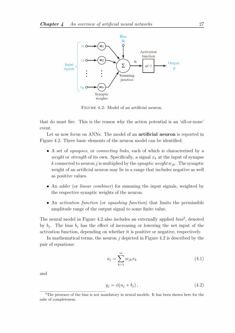
4.2 Model of an artificial neuron . . . . . . . . . . . . . . . . . . . . . . 25
4.3 Network architectures . . . . . . . . . . . . . . . . . . . . . . . . . . 28
4.4 The learning process . . . . . . . . . . . . . . . . . . . . . . . . . . 30
4.5 Unsupervised learning . . . . . . . . . . . . . . . . . . . . . . . . . 32
5 The self-organizing maps: SOM and TASOM 37
5.1 The SOM algorithm . . . . . . . . . . . . . . . . . . . . . . . . . . . 37
vi
5.1.1 Competition . . . . . . . . . . . . . . . . . . . . . . . . . . . 39
5.1.2 Cooperation . . . . . . . . . . . . . . . . . . . . . . . . . . . 39
5.1.3 Synaptic Adaptation . . . . . . . . . . . . . . . . . . . . . . 41
5.2 Summary of the SOM algorithm . . . . . . . . . . . . . . . . . . . . 42
5.3 Properties of the SOM . . . . . . . . . . . . . . . . . . . . . . . . . 43
5.4 The TASOM algorithm . . . . . . . . . . . . . . . . . . . . . . . . . 44
6 Time- and subject-adaptive dictionary for wearable devices 48
7 Results 52
7.1 Databases and performance metrics . . . . . . . . . . . . . . . . . . 52
7.2 Run-time analysis of the TASOM learning features during training . 54
7.3 Performance analysis of the time- and subject-adaptive compressionmethod - the choice of sf and L . . . . . . . . . . . . . . . . . . . . 59
7.4 Performance analysis of the time- and subject-adaptive compressionmethod - MIT-BIH Arrhythmia Database and MIMIC II Database . 65
8 Conclusions 69
vii
List of Figures
1.1 Wearable technology application chart. . . . . . . . . . . . . . . . . 4
3.1 Structure of the human heart. . . . . . . . . . . . . . . . . . . . . . 17
3.2 Schematic diagram of normal sinus rhythm for a human heart asseen on ECG. . . . . . . . . . . . . . . . . . . . . . . . . . . . . . . 17
3.3 Typical ECG trace. . . . . . . . . . . . . . . . . . . . . . . . . . . . 17
3.4 Typical PPG trace. . . . . . . . . . . . . . . . . . . . . . . . . . . . 17
4.1 Structure of two typical neurons. . . . . . . . . . . . . . . . . . . . . 26
4.2 Model of an artificial neuron. . . . . . . . . . . . . . . . . . . . . . . 27
4.3 Feed-forward network with a single layer of neurons. . . . . . . . . . 29
4.4 Multi-layer feed-forward network with one hidden layer and one out-put layer. . . . . . . . . . . . . . . . . . . . . . . . . . . . . . . . . 30
5.1 Example of a two dimensional lattice of neurons, shown for a threedimensional input and a four-by-four dimensional lattice. . . . . . . 38
5.2 Illustration of the learning process of a self-organizing map. . . . . . 44
6.1 Scheme of the lossy compression framework with time- and subject-adaptive dictionary. . . . . . . . . . . . . . . . . . . . . . . . . . . . 49
7.1 ECG signal: RMSE vs learning time for various sf . Trace 16786mfrom the MIT-BIH Normal Sinus Rhythm Database. L = 9. . . . . . 55
7.2 ECG signal: RMSE vs learning time for various codebook sizes.Trace 16786m from the MIT-BIH Normal Sinus Rhythm Database.sf = 10. . . . . . . . . . . . . . . . . . . . . . . . . . . . . . . . . . 55
7.3 ECG signal: RMSE vs learning time for different subjects from theMIT-BIH Arrhythmia Database. L = 9; sf = 10. . . . . . . . . . . . 56
7.4 ECG signal: RMSE vs learning time for a simulated non-stationarydistribution obtained by concatenating two different traces (101mand 113m from the MIT-BIH Arrhythmia Database). L = 9; sf = 10. 58
7.5 ECG signal: RMSE vs CR for various sf . Trace 113m from theMIT-BIH Arrhythmia Database. L = 9. . . . . . . . . . . . . . . . . 60
7.6 ECG signal: RMSE vs codebook size. Trace 113m from the MIT-BIH Arrhythmia Database. . . . . . . . . . . . . . . . . . . . . . . . 61
viii
7.7 ECG signal: RMSE vs CR for various codebook size. Trace 113mfrom the MIT-BIH Arrhythmia Database. . . . . . . . . . . . . . . . 61
7.8 ECG signal: RMSE vs energy consumption for compression for var-ious codebook size. Trace 113m from the MIT-BIH ArrhythmiaDatabase. . . . . . . . . . . . . . . . . . . . . . . . . . . . . . . . . 62
7.9 ECG signal: Updates per quarter-hour vs CR. Trace 113m from theMIT-BIH Arrhythmia Database. L = 9. . . . . . . . . . . . . . . . . 63
7.10 ECG signal: Quantized and original trace (113m from the MIT-BIHArrhythmia Database). L = 9. . . . . . . . . . . . . . . . . . . . . . 63
7.11 ECG signal: RMSE vs CR for different compression algorithms. . . . 66
7.12 ECG signal: RMSE vs energy consumption for compression for dif-ferent compression algorithms. . . . . . . . . . . . . . . . . . . . . . 67
7.13 ECG signal: RMSE vs total energy consumption for different com-pression algorithms. . . . . . . . . . . . . . . . . . . . . . . . . . . . 68
7.14 PPG signal: RMSE vs CR for different compression algorithms. . . . 68
ix

List of Tables
7.1 Cortex M4 processor features. . . . . . . . . . . . . . . . . . . . . . 53
x

Abbreviations
IoT Internet of Things
M2M Machine to Machine
MEMS Micro-Electro-Mechanical Systems
RFID Radio-Frequency IDentification
QoS Quality of Service
GPS Global Positioning System
ECG ElectroCardioGraphy, ElectroCardioGram
PPG PhotoPlethysmoGraphy, PhotoPlethysmoGram
EMG ElectroMyoGram
ABP Arterial Blood Pressure
RESP Respiratory
WSN Wireless Sensor Networks
WBSN Wireless Body Sensor Networks
PDA Personal Digital Assistant
SOM Self-Organizing Map
TASOM Time-Adaptive Self-Organizing Map
ANN Artificial Neural Network
VQ Vector Quantization, Vector Quantizer
LBG Linde-Buzo-Gray
KDD Knowledge Discovery in Databases
MSE Mean Squared Error
RMSE Root Mean Squared Error
CR Compression Ratio
RHS Right-Hand Side
MCU Micro-Controller Unit
CPU Central Processing Unit
xi


AcknowledgementsI would like to thank my supervisor Michele Rossi for his authoritative guidance
through the course of these months and Roberto Francescon, Matteo Gadaleta and
Mohsen Hooshmand for their precious advices and kind helpfulness.

Chapter 1
Introduction
1.1 The Internet of Things
Nowadays, according to the Internet World Stats [1], more than 3 billions people
around the world have access to the Internet and their number is continuing to
grow. From their personal computer, smartphone or tablet, typical online users
can browse the Web, send and receive emails, access and upload multimedia con-
tents, make VoIP calls, and edit profiles in social networks. It is predictable that,
within the next decade, the Internet will take a big leap forward, by enabling
an evolutionary as well as revolutionary class of applications and services based
on the widespread diffusion of spatially distributed devices with embedded iden-
tification, sensing, actuation and wireless communication capabilities. In such a
perspective, physical objects such as vehicles, gas and electric meters, appliances,
industrial equipment, and consumer electronics will become smart objects and will
bring into being pervasive, context-aware computing systems that collect informa-
tion from the background and act accordingly, using the Internet infrastructure for
data transfer and analytics. For the first time it will be possible to let things co-
operate with other things and more traditional networked digital machines, paving
the way to an optimized interaction with the environment around us. This is the
future as envisioned by the Internet of Things (IoT) paradigm [2] (in some cases
also referred to as Machine to Machine, or M2M, communication), fueled by the
recent advances in Micro-Electro-Mechanical Systems (MEMS), digital electronics,
wireless communications, energy harvesting, and hardware costs.
Unquestionably, the main strength of the IoT idea is the high impact it will
have on several aspects of everyday-life of potential beneficiaries. From the point
of view of a private user, the IoT introduction will translate into, e.g., domotics,
assisted living, and e-health. For business users, the most apparent consequences
will be visible in automation and industrial manufacturing, logistics, business and
process management, and intelligent transportation of people and goods. Many
challenging questions lie ahead and both technological and social knots have to
1
Chapter 1 Introduction 2
be untied before this can turn into reality [3]. Central issues are making a full
interoperability of heterogeneous interconnected devices possible and providing such
devices with an always higher degree of smartness that support their adaptation
and autonomous behavior, while meeting scalability requirements and guaranteeing
privacy and security. The things composing the IoT will be characterized by low
resources in terms of computation and energy capacity, therefore special attention
has to be paid to resource efficiency as well.
By inspecting some recent articles, we can sketch the following shared view
about the IoT progress. A major role in the identification and real-time tracking
of smart objects and in the mapping of the real world into the virtual one will be
played by Radio-Frequency IDentification (RFID) systems [4], which are composed
of one or more reader(s) and several RFID tags with unique ID. Tags, consisting of
small microchips attached to an antenna, are applied to objects (even persons or
animals) and queried by the readers, that generate an appropriate signal for trigger-
ing the transmission of IDs from tags in the surrounding area. The standardization
of the RFID technology and its coupling with sensor networks technologies, these
latter considered a pillar of the IoT, will allow to have unambiguously recogniz-
able tags and sensors inherently integrated into the environment. In order to fully
exploit the advantages brought by Internet connectivity, such as contents sharing
and location-independent access to data, scalable addressing policies and commu-
nication protocols that cope with the devices’ diversity must be devised. Although
rules that manage the relationship between RFID tags’ IDs and IPv6 addresses
have been already proposed and there’s no lack for wireless communication pro-
tocols (think of ZigBee, Bluetooth, and Wi-Fi), the fragmentation characterizing
the existing procedures may hamper objects interoperability and can slow down
the conception of a coherent reference model for the IoT. Further investigations
also need to be done for traffic characterization and data management, both fun-
damental to network providers to plan the expansion of their platforms and the
support of Quality of Service (QoS), to assure authentication and data integrity
against unauthorized accesses and malicious attacks, and to endow objects with
self-organization tools that anticipate user needs and tune decisions and actions
to different situations. At any mentioned design level, technicians and engineerss
have to pay special attention to energy-optimization. New, compact energy storage
sources coupled with energy transmission and harvesting methods, as well as ex-
tremely low-power circuitry and energy-efficient architectures and protocol suites,
will be key factors for the roll out of autonomous wireless smart systems.
In order to promote IoT as a publicly acknowledged and implemented paradigm,
the proposed solutions should not be derived from scratch and independently of each
other but rather pursuing a holistic approach that aims at unifying the existing and
upcoming efforts and technologies into an ubiquitously applicable framework. Open
and flexible interfaces and appropriate bridges could then leverage the differences
between devices and services and let them collaborate in a globally integrated
Chapter 1 Introduction 3
system, where many subsystems (‘INTRAnets’) of Things are joined together in a
true ‘INTERnet’ of Things [5].
1.2 Wearable devices
Wearable devices are a leading category in the IoT, whose development and mar-
ket penetration have experienced an astonishing growth since late 2000. They can
be broadly defined as miniature embedded computing systems equipped with a
range of sensors, processing and communication modules1 and having the distinc-
tive property to be worn by people. Besides handheld devices, wearables extend
the IoT paradigm to a human-centric sensing scenario where sensors are not only
integrated into the environment but we, as humans, carry ourselves the sensing
devices and actively participate in the sensing phase. As emphasized by Srivastava
et al. in [6], human involvement makes it feasible to get even more information dur-
ing the study of processes in complex personal, social and urban spaces than that
available using traditional Wireless Sensor Networks (WSNs) or static smart things.
By taking advantage of people who already live, work and travel in these spaces,
human-centric sensing can overcome gaps in spatio-temporal coverage and inability
to adapt to dynamic and cluttered areas. Measurement traces from accelerometers,
gyroscopes, magnetometers, thermometers, cameras, and GPS trackers, which can
now be found in many consumer-grade smartphones or wearable devices, can be
used to obtain a geo-stamped time series of one’s mobility pattern and transporta-
tion mode, supplemented by a detailed description of local conditions. Such streams
of data might be recorded through lifelogging mobile apps, which enable the user
to derive personal statistics and to publish meaningful events and memories in so-
cial networks; they can be submitted to web-services that manage the real-time
monitoring of issues of interest; they can be collected from specialized campaigns
for computing community statistics or mapping physical and social phenomena.
Compared with their handheld counterpart, wearable devices such as wrist-
bands, smart watches, chest straps, skin patches and clip-on devices claim er-
gonomicity, dimension reduction (at least in the majority of the cases), and better
fine-grain collection capabilities, given their closer proximity to the human body
and the purpose-specific design of shapes, sensors and processing tools [7]. Accord-
ing to forecasts, the wearable business will power from 20 billion in 2015 to almost
70 billion in 2025 [8], involving healthcare, security, entertainment, industrial, and
tactical applications (see Figure 1.1). In particular, the healthcare sector (merging
fitness, wellness and medical) is expected to dominate, playing on the aforemen-
tioned wearable features, which become extremely valuable when a uninterrupted,
non invasive, personalized service that tracks activity and physiological signals is
1Typically, wearables have low-power wireless communication interfaces such as BluetoothSmart (also referred to as BlueTooth Low Energy, or BTLE), low-power Wi-Fi or ZigBee (basedon IEEE 802.15.4 standard).
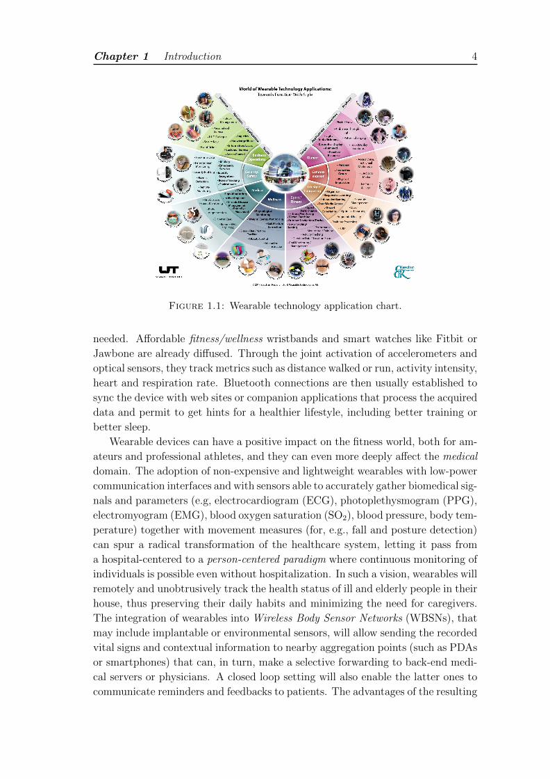
Chapter 1 Introduction 4
Figure 1.1: Wearable technology application chart.
needed. Affordable fitness/wellness wristbands and smart watches like Fitbit or
Jawbone are already diffused. Through the joint activation of accelerometers and
optical sensors, they track metrics such as distance walked or run, activity intensity,
heart and respiration rate. Bluetooth connections are then usually established to
sync the device with web sites or companion applications that process the acquired
data and permit to get hints for a healthier lifestyle, including better training or
better sleep.
Wearable devices can have a positive impact on the fitness world, both for am-
ateurs and professional athletes, and they can even more deeply affect the medical
domain. The adoption of non-expensive and lightweight wearables with low-power
communication interfaces and with sensors able to accurately gather biomedical sig-
nals and parameters (e.g, electrocardiogram (ECG), photoplethysmogram (PPG),
electromyogram (EMG), blood oxygen saturation (SO2), blood pressure, body tem-
perature) together with movement measures (for, e.g., fall and posture detection)
can spur a radical transformation of the healthcare system, letting it pass from
a hospital-centered to a person-centered paradigm where continuous monitoring of
individuals is possible even without hospitalization. In such a vision, wearables will
remotely and unobtrusively track the health status of ill and elderly people in their
house, thus preserving their daily habits and minimizing the need for caregivers.
The integration of wearables into Wireless Body Sensor Networks (WBSNs), that
may include implantable or environmental sensors, will allow sending the recorded
vital signs and contextual information to nearby aggregation points (such as PDAs
or smartphones) that can, in turn, make a selective forwarding to back-end medi-
cal servers or physicians. A closed loop setting will also enable the latter ones to
communicate reminders and feedbacks to patients. The advantages of the resulting
Chapter 1 Introduction 5
tele-medicine or, better, mobile health (m-health) infrastructure are multifold and
will be quantifiable in terms of improved prevention, early diagnosis, care’s cus-
tomization and quality, increased patient autonomy and mobility and last, but not
least, reduced healthcare costs. Many concrete examples of the m-health potential
are illustrated in [9]. To name a few, life-threatening situations can be far more
likely detected in time, chronic conditions (e.g., those associated with cognitive dis-
orders like Alzheimer’s or Parkinson’s) can be optimally maintained, physical reha-
bilitations and recovery periods after acute events (such as myocardial infarction)
or surgical procedures can be supervised after shorter hospital stays, adherence to
treatment guidelines and effects of drug therapies can be verified, all of this in real-
time and avoiding unnecessary interventions by the medical stuff. Moreover, if we
let the person-centered paradigm extend over clinics and hospitals, wearables can
contribute to simplify the bulky and typically wired monitoring systems in there
and to monitor ambulatory in-patients around the clock, helping doctors to spot
early signs of deterioration.
1.3 Motivation and contribution
In order to reap the full benefits of wearables-based systems, especially those suited
to healthcare applications, and to seamlessly integrate them into the IoT scenario,
many technical hurdles still remain to be addressed. One of the paramount issues,
concerning the whole IoT scenario but especially smart wearable objects, is energy
optimization. The wearable nature necessitates a vanishingly small size and weight
and, as a result, these devices have limited hardware resources and power bud-
get. Research efforts are thus indispensable to supply them with energy-efficient
processing tools and communication protocols that optimally manage their limited
battery life and constrained memory, while guaranteeing all the requirements on
reliable and timely message delivery [7].
This thesis is focused on the lightweight compression of biomedical signals for
reducing memory and transmission costs of wearables in finegrained monitoring
applications, such those related to the healthcare sector. Although a great num-
ber of compression techniques have appeared in the literature, the search for new
methods continues, with the aim of achieving greater compression ratios (CR) with
low-power processing tools, while preserving the clinical information content in the
reconstructed signal. I propose a novel lossy compression scheme based on Artifi-
cial Neural Networks (ANNs) (specifically, the neural network called Time-Adaptive
Self-Organizing Map - TASOM), motif extraction, and Vector Quantization (VQ).
The reference scenario consists of a wearable device recording a biomedical signal
with a certain degree of periodicity (such as ECG and PPG) from a subject and
wirelessly transmitting it to an aggregation point. The acquired signal is decom-
posed into segments corresponding to a signal pseudo-period. A preliminary train-
ing phase uses the incoming segments to let the TASOM learn the actual subject’s
Chapter 1 Introduction 6
signal distribution. The synaptic weights of the TASOM’s neurons become progres-
sively and adaptively tuned to approximate such distribution, without any prior
knowledge upon it. At the end of the preliminary training phase, the subject-based
codebook of segments is defined as the one formed by the neurons’ synaptic weights,
thus representing the codebook’s codewords. Each new unseen segment is coded
through a VQ approach which selects the best matching codeword through a fast
codebook search algorithm and transmits its index to the receiving node, which has
a copy of the codebook at the transmitter available. Each new segment is also used
to further train the TASOM in an online fashion so as to maintain a representative
codebook at all times.
The contents of this thesis are organized as follows. In the next Chapter 2, I
illustrate the literary work related to the new compression method. In Chapter
3 I provide a review of the basic concepts of motif extraction and VQ, detailing
how motif extraction has been applied to biomedical signals and reporting the
fast codebook search algorithm I used for finding the best matching codeword
during the quantization process. In Chapter 4 I sum up the fundamental notions
about ANNs and then, in Chapter 5, I elucidate the Self-Organizing Map (SOM)
learning algorithm and its time-adaptive version (i.e., the TASOM), underlying the
advantages of the latter with respect to the basic SOM. In Chapter 6 I describe the
whole compression framework and in Chapter 7, I present a quantitative analysis
of compression and fidelity performance, showing the improvements with respect
to more traditional approaches. Finally, in Chapter 8 I draw the conclusions.
Chapter 2
Related work
In this thesis, I consider signal compression as a means to boost the battery life of
wearables in real-time monitoring applications. By remove data redundancy, com-
pression actually makes it possible to limit the amount of information to store and
transmit, entailing substantial energy savings and lighter traffic toward aggregation
points and Internet servers.
In the last decades, quite a few lossy and lossless compression algorithms for
ECG signals, probably the most important for the diagnosis of heart malfunc-
tions, have been proposed in the literature. They are classifiable into three main
categories: Direct Methods, Transformation Methods and Parameter Extraction
Methods.
Direct methods, among which we have the Lightweight Temporal Compression
(LTC) [10], the Amplitude Zone Time Epoch Coding (AZTEC) [11], and the Co-
ordinate Reduction Time Encoding System (CORTES) [12], operate in the time
domain and utilize prediction or interpolation algorithms to reduce redundancy
in an input signal by examining a successive number of neighboring samples. In
particular, AZTEC exploits the Zero-Order Interpolator (ZOI) to convert the ECG
samples into a sequence of plateaus and slopes. CORTES uses AZTEC for the low
frequency regions of the ECG signal, while it simply discards one sample out of
two consecutive samples in high frequency regions. LTC substitutes the ECG time
series with a sequence of segments delimited by two original samples and defined
according to a predetermined error threshold.
Though such algorithms generally have a low complexity, the reconstruction qual-
ity for a given compression often result to be worse than that of transformation
methods, due to the piecewise character of the approximations [13].
Transformation methods perform a linear orthogonal transformation, such as
Fast Fourier Transform (FFT) [14], Discrete Cosine Transform (DCT) [15], and
Discrete Wavelet Transform (DWT) [16], of the input signal and select a number
of transform coefficients to represent the original samples. The amount of com-
pression depends on the number of coefficients that are selected, the representation
accuracy depends on how many and which coefficients are retained. The schemes
7
Chapter 2 Related work 8
belonging to this class can provide high CR with limited distortion. However, their
computational complexity is typically too high for wearable devices [17].
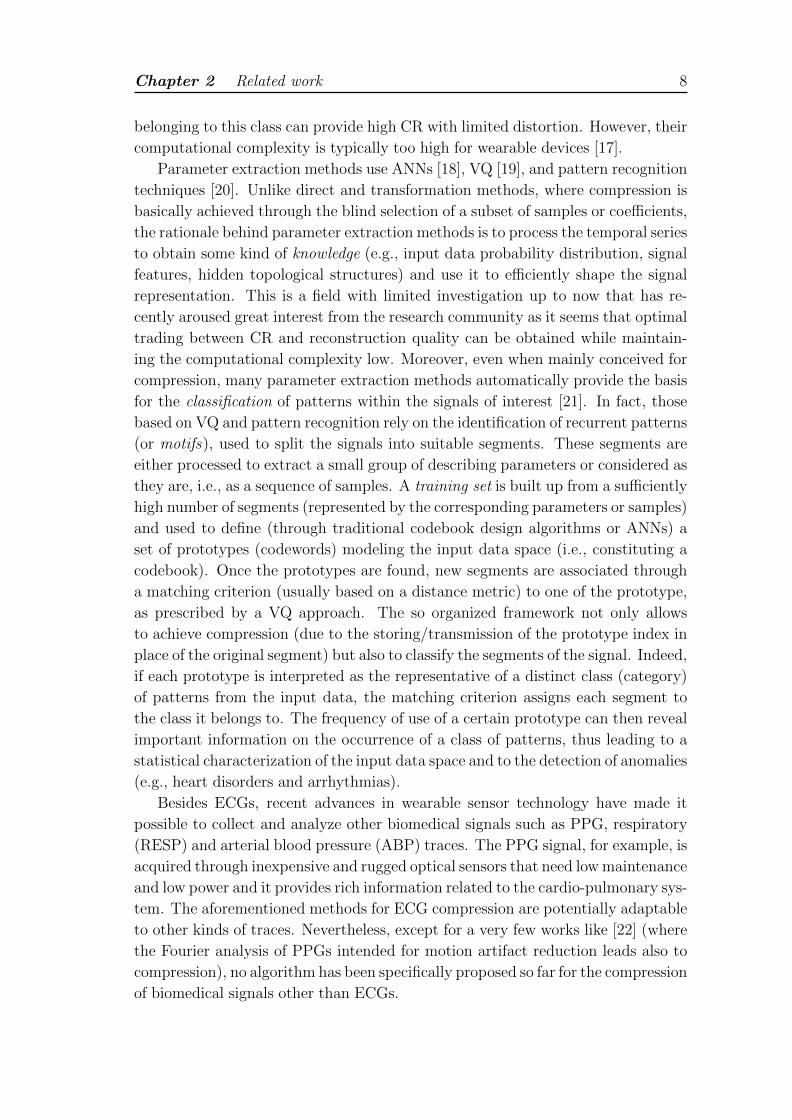
Parameter extraction methods use ANNs [18], VQ [19], and pattern recognition
techniques [20]. Unlike direct and transformation methods, where compression is
basically achieved through the blind selection of a subset of samples or coefficients,
the rationale behind parameter extraction methods is to process the temporal series
to obtain some kind of knowledge (e.g., input data probability distribution, signal
features, hidden topological structures) and use it to efficiently shape the signal
representation. This is a field with limited investigation up to now that has re-
cently aroused great interest from the research community as it seems that optimal
trading between CR and reconstruction quality can be obtained while maintain-
ing the computational complexity low. Moreover, even when mainly conceived for
compression, many parameter extraction methods automatically provide the basis
for the classification of patterns within the signals of interest [21]. In fact, those
based on VQ and pattern recognition rely on the identification of recurrent patterns
(or motifs), used to split the signals into suitable segments. These segments are
either processed to extract a small group of describing parameters or considered as
they are, i.e., as a sequence of samples. A training set is built up from a sufficiently
high number of segments (represented by the corresponding parameters or samples)
and used to define (through traditional codebook design algorithms or ANNs) a
set of prototypes (codewords) modeling the input data space (i.e., constituting a
codebook). Once the prototypes are found, new segments are associated through
a matching criterion (usually based on a distance metric) to one of the prototype,
as prescribed by a VQ approach. The so organized framework not only allows
to achieve compression (due to the storing/transmission of the prototype index in
place of the original segment) but also to classify the segments of the signal. Indeed,
if each prototype is interpreted as the representative of a distinct class (category)
of patterns from the input data, the matching criterion assigns each segment to
the class it belongs to. The frequency of use of a certain prototype can then reveal
important information on the occurrence of a class of patterns, thus leading to a
statistical characterization of the input data space and to the detection of anomalies
(e.g., heart disorders and arrhythmias).
Besides ECGs, recent advances in wearable sensor technology have made it
possible to collect and analyze other biomedical signals such as PPG, respiratory
(RESP) and arterial blood pressure (ABP) traces. The PPG signal, for example, is
acquired through inexpensive and rugged optical sensors that need low maintenance
and low power and it provides rich information related to the cardio-pulmonary sys-
tem. The aforementioned methods for ECG compression are potentially adaptable
to other kinds of traces. Nevertheless, except for a very few works like [22] (where
the Fourier analysis of PPGs intended for motion artifact reduction leads also to
compression), no algorithm has been specifically proposed so far for the compression
of biomedical signals other than ECGs.
Chapter 2 Related work 9
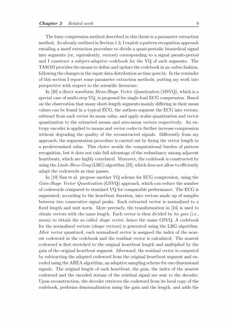
The lossy compression method described in this thesis is a parameter extraction
method. As already outlined in Section 1.3, I exploit a pattern recognition approach
entailing a motif extraction procedure to divide a quasi-periodic biomedical signal
into segments (or, equivalently, vectors) corresponding to a signal pseudo-period
and I construct a subject-adaptive codebook for the VQ of such segments. The
TASOM provides the means to define and update the codebook in an online fashion,
following the changes in the input data distribution as time goes by. In the reminder
of this section I report some parameter extraction methods, putting my work into
perspective with respect to the scientific literature.
In [20] a direct waveform Mean-Shape Vector Quantization (MSVQ), which is a
special case of multi-step VQ, is proposed for single-lead ECG compression. Based
on the observation that many short-length segments mainly differing in their mean
values can be found in a typical ECG, the authors segment the ECG into vectors,
subtract from each vector its mean value, and apply scalar quantization and vector
quantization to the extracted means and zero-mean vectors respectively. An en-
tropy encoder is applied to means and vector codes to further increase compression
without degrading the quality of the reconstructed signals. Differently from my
approach, the segmentation procedure is carried out by fixing the vector length to
a predetermined value. This choice avoids the computational burden of pattern
recognition, but it does not take full advantage of the redundancy among adjacent
heartbeats, which are highly correlated. Moreover, the codebook is constructed by
using the Linde-Buzo-Gray (LBG) algorithm [23], which does not allow to efficiently
adapt the codewords as time passes.
In [19] Sun et al. propose another VQ scheme for ECG compression, using the
Gain-Shape Vector Quantization (GSVQ) approach, which can reduce the number
of codewords compared to standard VQ for comparable performance. The ECG is
segmented, according to the heartbeat duration, into vectors made up of samples
between two consecutive signal peaks. Each extracted vector is normalized to a
fixed length and unit norm. More precisely, the transformation in [24] is used to
obtain vectors with the same length. Each vector is then divided by its gain (i.e.,
norm) to obtain the so called shape vector, hence the name GSVQ. A codebook
for the normalized vectors (shape vectors) is generated using the LBG algorithm.
After vector quantized, each normalized vector is assigned the index of the near-
est codeword in the codebook and the residual vector is calculated. The nearest
codeword is first stretched to the original heartbeat length and multiplied by the
gain of the original heartbeat segment. Afterward, the residual vector is computed
by subtracting the adapted codeword from the original heartbeat segment and en-
coded using the AREA algorithm, an adaptive sampling scheme for one dimensional
signals. The original length of each heartbeat, the gain, the index of the nearest
codeword and the encoded stream of the residual signal are sent to the decoder.
Upon reconstruction, the decoder retrieves the codeword from its local copy of the
codebook, performs denormalization using the gain and the length, and adds the
Chapter 2 Related work 10
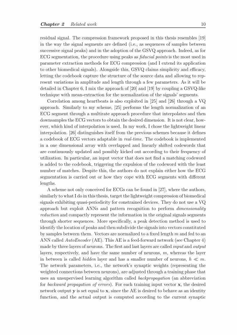
residual signal. The compression framework proposed in this thesis resembles [19]
in the way the signal segments are defined (i.e., as sequences of samples between
successive signal peaks) and in the adoption of the GSVQ approach. Indeed, as for
ECG segmentation, the procedure using peaks as fiducial points is the most used in
parameter extraction methods for ECG compression (and I extend its application
to other biomedical signals). Alongside this, GSVQ claims simplicity and efficacy,
letting the codebook capture the structure of the source data and allowing to rep-
resent variations in amplitude and length through a few parameters. As it will be
detailed in Chapter 6, I mix the approach of [20] and [19] by coupling a GSVQ-like
technique with mean-extraction for the normalization of the signals’ segments.
Correlation among heartbeats is also exploited in [25] and [26] through a VQ
approach. Similarly to my scheme, [25] performs the length normalization of an
ECG segment through a multirate approach procedure that interpolates and then
downsamples the ECG vectors to obtain the desired dimension. It is not clear, how-
ever, which kind of interpolation is used. In my work, I chose the lightweight linear
interpolation. [26] distinguishes itself from the previous schemes because it defines
a codebook of ECG vectors adaptable in real-time. The codebook is implemented
in a one dimensional array with overlapped and linearly shifted codewords that
are continuously updated and possibly kicked out according to their frequency of
utilization. In particular, an input vector that does not find a matching codeword
is added to the codebook, triggering the expulsion of the codeword with the least
number of matches. Despite this, the authors do not explain either how the ECG
segmentation is carried out or how they cope with ECG segments with different
lengths.
A scheme not only conceived for ECGs can be found in [27], where the authors,
similarly to what I do in this thesis, target the lightweight compression of biomedical
signals exhibiting quasi-periodicity for constrained devices. They do not use a VQ
approach but exploit ANNs and pattern recognition to perform dimensionality
reduction and compactly represent the information in the original signals segments
through shorter sequences. More specifically, a peak detection method is used to
identify the location of peaks and then subdivide the signals into vectors constituted
by samples between them. Vectors are normalized to a fixed length m and fed to an
ANN called AutoEncoder (AE). This AE is a feed-forward network (see Chapter 4)
made by three layers of neurons. The first and last layers are called input and output
layers, respectively, and have the same number of neurons, m, whereas the layer
in between is called hidden layer and has a smaller number of neurons, h � m.
The network parameters, i.e., the network’s synaptic weights (representing the
weighted connections between neurons), are adjusted through a training phase that
uses an unsupervised learning algorithm called backpropagation (an abbreviation
for backward propagation of errors). For each training input vector x, the desired
network output y is set equal to x, since the AE is desired to behave as an identity
function, and the actual output is computed according to the current synaptic
Chapter 2 Related work 11
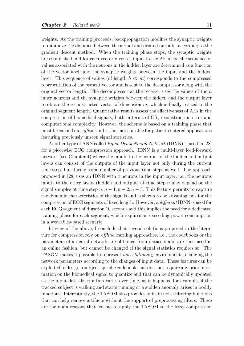
weights. As the training proceeds, backpropagation modifies the synaptic weights
to minimize the distance between the actual and desired outputs, according to the
gradient descent method. When the training phase stops, the synaptic weights
are established and for each vector given as input to the AE a specific sequence of
values associated with the neurons in the hidden layer are determined as a function
of the vector itself and the synaptic weights between the input and the hidden
layer. This sequence of values (of length h � m) corresponds to the compressed
representation of the present vector and is sent to the decompressor along with the
original vector length. The decompressor at the receiver uses the values of the h
inner neurons and the synaptic weights between the hidden and the output layer
to obtain the reconstructed vector of dimension m, which is finally resized to the
original segment length. Quantitative results assess the effectiveness of AEs in the
compression of biomedical signals, both in terms of CR, reconstruction error and
computational complexity. However, the scheme is based on a training phase that
must be carried out offline and is thus not suitable for patient-centered applications
featuring previously unseen signal statistics.
Another type of ANN called Input-Delay Neural Network (IDNN) is used in [28]
for a piecewise ECG compression approach. IDNN is a multi-layer feed-forward
network (see Chapter 4) where the inputs to the neurons of the hidden and output
layers can consist of the outputs of the input layer not only during the current
time step, but during some number of previous time steps as well. The approach
proposed in [28] uses an IDNN with 4 neurons in the input layer, i.e., the neurons
inputs to the other layers (hidden and output) at time step n may depend on the
signal samples at time step n, n− 1, n− 2, n− 3. This feature permits to capture
the dynamic characteristics of the signals and is shown to be advantageous for the
compression of ECG segments of fixed length. However, a different IDNN is used for
each ECG segment of duration 10 seconds and this implies the need for a dedicated
training phase for each segment, which requires an exceeding power consumption
in a wearables-based scenario.
In view of the above, I conclude that several solutions proposed in the litera-
ture for compression rely on offline learning approaches, i.e., the codebooks or the
parameters of a neural network are obtained from datasets and are then used in
an online fashion, but cannot be changed if the signal statistics requires so. The
TASOM makes it possible to represent non-stationary environments, changing the
network parameters according to the changes of input data. These features can be
exploited to design a subject-specific codebook that does not require any prior infor-
mation on the biomedical signal to quantize and that can be dynamically updated
as the input data distribution varies over time, as it happens, for example, if the
tracked subject is walking and starts running or a sudden anomaly arises in bodily
functions. Interestingly, the TASOM also provides built-in noise-filtering functions
that can help remove artifacts without the support of preprocessing filters. These
are the main reasons that led me to apply the TASOM to the lossy compression

Chapter 2 Related work 12
of biomedical signals, together with the crucial factor that the TASOM learning
algorithm makes it possible to outperform other compression methods in terms of
energy efficiency.
Chapter 3
Motif extraction
and vector quantization
Motif extraction, VQ, and the TASOM are the key tools used to implement the
proposed compression method. In the following, I outline the basic concepts of
motif extraction and VQ and I describe the rationale behind the choice of these
techniques for the lossy compression of biomedical signals.
3.1 Motif extraction
3.1.1 Basic concepts
In computer science, data mining, also known as Knowledge Discovery in Databases
(KDD), is the interdisciplinary scientific field concerned with the automatic or
semi-automatic extraction of useful patterns from large data sets (or databases)
for summarization, visualization, better analysis or prediction purposes. In the
last decades, the problem of efficiently locating previously known patterns in a
database has received much attention and may now largely be regarded as solved.
A problem that needs further investigation and that is more interesting from a
knowledge discovery viewpoint, is the detection of previously unknown, frequently
occurring patterns. Such patterns can be referred to as primitive shapes, recurrent
patterns or motifs. I refer to this last definition, attributed to Keogh et al. [29],
that borrowed the term from computational biology, where a sequence motif is a
recurring DNA pattern that is presumed to have a biological significance.
The fundamentals of motif extraction can be summed up as follows [29]:
1. Given a time series xxx = [x1, x2, . . . , xr]T , xk ∈ R, k = 1, 2, . . . , r, a subse-
quence xxxp with length m of xxx is defined as:
xxxp = [xp, xp+1, . . . , xp+m−1]T , 1 ≤ p ≤ r −m+ 1 . (3.1)
13
Chapter 3 Motif extraction and vector quantization 14
2. Given a distance metric D(·) and a predetermined threshold ε ∈ R+, a sub-
sequence xxxp2 is said to be a matching subsequence of xxxp1 if
D(xxxp1 ,xxxp2) ≤ ε . (3.2)
If condition (3.2) is satisfied, then there exists a match between xxxp2 and xxxp1 .
3. Given a subsequence xxxp1 and a matching subsequence xxxp2 , xxxp2 is a trivial
match to xxxp1 if either p1 ≡ p2 or there does not exist a subsequence xxxp3 such
that D(xxxp1 ,xxxp3) > ε, and either p1 < p3 < p2 or p2 < p3 < p1.
4. The most significant motif in xxx (called 111-Motif) is the subsequence, denoted
by CCC1, that has the highest count of non-trivial matches. The Kth most sig-
nificant motif in xxx (calledKKK-Motif) is the subsequence, denoted asCCCK , that
has the highest count of non-trivial matches and satisfies D(CCCK ,CCCi) > 2ε,
for all 1 ≤ i < K, where CCCi is the i-Motif. This last requirement forces the
set of subsequences non trivially matched to a given motif to be mutually
exclusive.
5. In the above scenario, motif extraction can be defined as the procedure
that aims at locating a given K-Motif in the time series, and the set of all the
subsequences that match it.
3.1.2 Motif extraction in biomedical signals
The compression framework proposed in this thesis targets biomedical signals ac-
quired by a wearable device. A biomedical signal is any signal generated from the
human body’s activity (e.g., heart activity, brain activity or lungs activity) that
can be continually measured and monitored. It can be of chemical, electrical, me-
chanical, magnetic nature and is typically collected as voltages or currents through
specific transducers. Due to the intrinsically cyclic behavior of heart and breathing
activity, many biomedical signals such as the ECG, PPG, RESP and ABP signal,
are oscillatory in nature, though not exactly periodic in a strict mathematical sense:
by looking at the time evolution of these signals, one can observe a concatenation of
sequences with similar morphology (i.e., with similar length, shape and amplitude)
that, however, never identically reproduce themselves. Such biomedical signals ex-
hibit the quasi-periodicity property (or, equivalently, are quasi-periodic signals). A
continuous quasi-periodic signal x(t) can be formally defined as a signal that
satisfies the condition
x(t) = x(t+ T + ∆T ) + ∆x, ∆x,∆T ∈ R, t, T ∈ R+ ∪ {0} , (3.3)
where T is the fundamental period and ∆T and ∆x are random variables represent-
ing, respectively, time and amplitude variations and in general, but non necessarily,
Chapter 3 Motif extraction and vector quantization 15
satisfying |∆T | � T and |∆x| � max(x(t))−min(x(t)).1 Analogously, in the dis-
crete time domain, a quasi-periodic signal x(n) satisfies:
x(n) = x(n+ T + ∆T ) + ∆x, ∆x ∈ R, ∆T ∈ Z, n, T ∈ N . (3.4)
I only take into consideration (discrete) quasi-periodic biomedical signals, whose
quasi-periodicity (and thus correlation among subsequent cycles) is leveraged to
reach high CRs through the joint exploitation of motif extraction and vector quan-
tization.
With respect to motif extraction, I define as motif a subsequence of the quasi-
periodic biomedical signal made up of consecutive samples in a pseudo-period (i.e.,
in the time interval T + ∆T ), without discriminating between K-Motifs, as they
are defined in Sub-section 3.1.1. In a quasi-periodic signal there is no need for
a learning phase that discovers the most recurrent patterns (or motifs) because
the quasi-periodicity allows by itself to state that there is a unique recurrent pat-
tern, that it coincides with any subsequence associated with a pseudo-period of
length T+∆T and that all the consecutive, non-overlapping subsequences of length
T + ∆T can be considered to be matching subsequences. As a consequence, the
motif extraction phase in this thesis simply consists in segmenting the considered
biomedical signal in subsequences of length T + ∆T . The randomness of variable
∆T , which can be thought of to be a major issue, does not need to be analytically
characterized to correctly perform the segmentation. Indeed, as it will be made
clearer by the following examples, the presence of peaks in the signals makes peak
detection the only true requirement for a proper segmentation, and peak detection
is a problem already deeply investigated in the literature that can be solved through
well established algorithms.
3.1.3 Quasi-periodic biomedical signals: examples
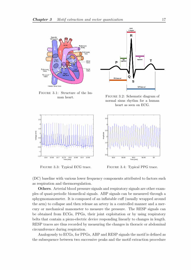
ECG. The heart is a specialised muscle that pumps blood throughout the body
through the blood vessels (arteries, veins and capillaries) of the circulatory system,
supplying oxygen and nutrients to the tissues and removing carbon dioxide and
other metabolic wastes. The structure of a human heart comprises four chambers,
as shown in Figure 3.1: two upper chambers (the right and the left atrium) and
two lower ones (the right and the left ventricle). The heart activity follows a cyclic
pattern, during which the cardiac cycle repeats itself with every heartbeat. The
normal rhythmical heartbeat, called sinus rhythm, is established by the sinoatrial
node, the heart’s natural pacemaker in the upper part of the right atrium. Here
an electrical signal is created that travels through the heart, causing it to contract
and begin the cardiac cycle. During this cycle, de-oxygenated blood transported
by veins passes from the right atrium to the right ventricle and then thorugh the
1max(x(t)) and min(x(t)) stand for the maximum and minimum values assumed by the signalamplitude, respectively.
Chapter 3 Motif extraction and vector quantization 16
lungs where carbon dioxide is released and oxygen is absorbed. At the same time,
the blood that has been oxygenated in the previous cycle enters the left atrium,
passes through the left ventricle and is pumped through the aorta and arteries to
the rest of the body. The frequency of heartbeats is measured by the heart rate,
generally expressed as beats per minute (bpm). The normal resting adult human
heart rate ranges from 60 to 100 bpm.
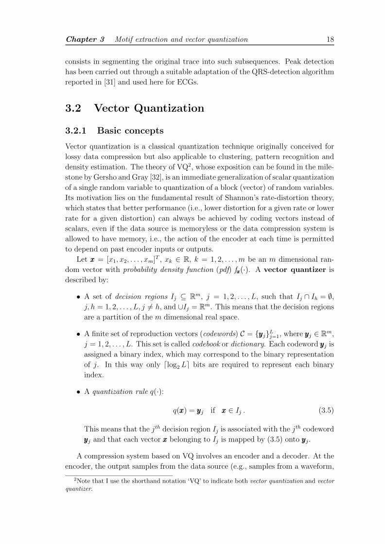
The ECG records the heart’s electrical activity for the diagnosis of heart mal-
functions using electrodes placed on the body’s surface. As shown in Figure 3.2,
in a typical ECG lead of a healthy person each cardiac cycle is represented by the
succession of five waves, namely P-, Q-, R-, S-, T-wave, among which the QRS
complex (which captures the ventricular depolarization leading to ventricular con-
traction) forms a special group. The duration, amplitude, and morphology of these
waves, especially those of the QRS complex, are useful in diagnosing cardiovascular
diseases. In particular, the most high frequency component, called R peak, is used
to keep track of the heart rate and thus to assess heart rhythm regularity.
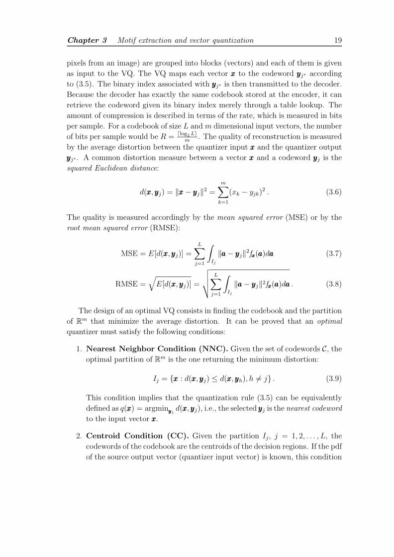
Given the heart rhythmicity (see Figure 3.3), the ECG can be classified as a
quasi-periodic biomedical signal. When the compression method proposed in this
thesis is to be applied to ECG traces, I segment them into subsequences made
up of consecutive samples between successive R peaks. Therefore a subsequence
between two R peaks represents the motif of an ECG. I do not segment the ECG
trace according to the natural partition induced by the cardiac cycles because such
approach would introduce the hurdle of locating the correct extremes of each cycle,
whereas R peaks are clearly defined and a variety of algorithms, whose accuracy
have been extensively tested, are available in the literature to perform peak de-
tection. In particular, the Pan-Tompkins real-time QRS-detection algorithm [30],
which uses a processing sequence made by bandpass filtering, differentiation, squar-
ing and moving window integration, remains, until today, a very robust method
to locate the R peaks. Notwithstanding this, I preferred the fast QRS-detection
algorithm proposed in [31], which is especially targeted for battery-driven devices
due to its lightweight character.
PPG. Photoplethysmography is a simple and low-cost optical technique used to
detect blood volume changes in the microvascular bed of tissue. The pulse oxime-
ter is a non-invasive device commonly used to record a PPG signal, from which
heart rate, blood pressure and also RESP signals can be computed. It detects vol-
ume changes caused by the heart pounding by illuminating the skin with the light
from a light-emitting diode (LED) and then measuring the amount of light either
transmitted or reflected to a photodiode. By varying the wavelenght of the light
emitted by the LED, pulse oximeters can also measure blood oxygen saturation.
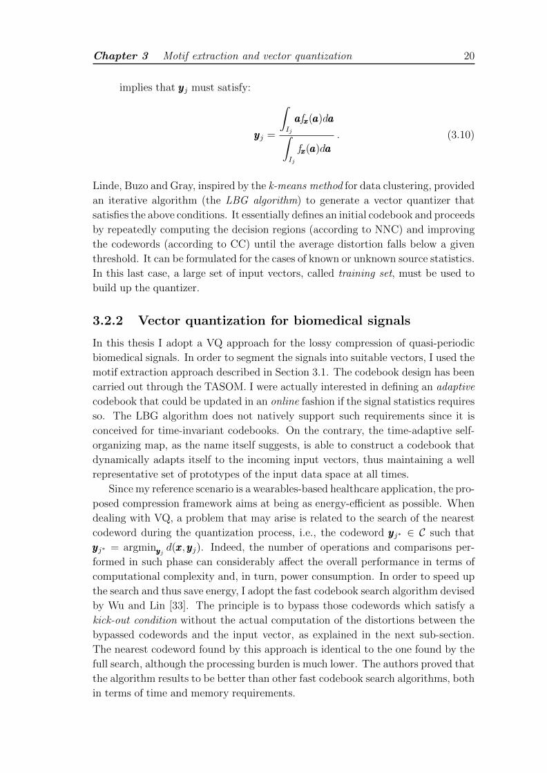
As shown in Figure 3.4, a typical PPG signal is a quasi-periodic biomedical signal
that comprises a pulsatile (AC) physiological waveform attributed to cardiac syn-
chronous changes in the blood volume with each heartbeat and a slowly varying
Chapter 3 Motif extraction and vector quantization 17
Figure 3.1: Structure of the hu-man heart. Figure 3.2: Schematic diagram of
normal sinus rhythm for a humanheart as seen on ECG.
10.6 10.65 10.7 10.75 10.8 10.85 10.9 10.95−1.5
−1
−0.5
0
0.5
1
1.5
2
2.5
3
Time [min]
Vol
tage
[mV
]
Figure 3.3: Typical ECG trace.
58.8 58.85 58.9 58.95 59
0.5
1
1.5
2
2.5
3
3.5
Time [min]
Am
plitu
de
Figure 3.4: Typical PPG trace.
(DC) baseline with various lower frequency components attributed to factors such
as respiration and thermoregulation.
Others. Arterial blood pressure signals and respiratory signals are other exam-
ples of quasi-periodic biomedical signals. ABP signals can be measured through a
sphygmomanometer. It is composed of an inflatable cuff (usually wrapped around
the arm) to collapse and then release an artery in a controlled manner and a mer-
cury or mechanical manometer to measure the pressure. The RESP signals can
be obtained from ECGs, PPGs, their joint exploitation or by using respiratory
belts that contain a piezo-electric device responding linearly to changes in length.
RESP traces are thus recorded by measuring the changes in thoracic or abdominal
circumference during respiration.
Analogously to ECGs, for PPGs, ABP and RESP signals the motif is defined as
the subsequence between two successive peaks and the motif extraction procedure
Chapter 3 Motif extraction and vector quantization 18
consists in segmenting the original trace into such subsequences. Peak detection
has been carried out through a suitable adaptation of the QRS-detection algorithm
reported in [31] and used here for ECGs.
3.2 Vector Quantization
3.2.1 Basic concepts
Vector quantization is a classical quantization technique originally conceived for
lossy data compression but also applicable to clustering, pattern recognition and
density estimation. The theory of VQ2, whose exposition can be found in the mile-
stone by Gersho and Gray [32], is an immediate generalization of scalar quantization
of a single random variable to quantization of a block (vector) of random variables.
Its motivation lies on the fundamental result of Shannon’s rate-distortion theory,
which states that better performance (i.e., lower distortion for a given rate or lower
rate for a given distortion) can always be achieved by coding vectors instead of
scalars, even if the data source is memoryless or the data compression system is
allowed to have memory, i.e., the action of the encoder at each time is permitted
to depend on past encoder inputs or outputs.
Let xxx = [x1, x2, . . . , xm]T , xk ∈ R, k = 1, 2, . . . ,m be an m dimensional ran-
dom vector with probability density function (pdf) fxxx(·). A vector quantizer is
described by:
• A set of decision regions Ij ⊆ Rm, j = 1, 2, . . . , L, such that Ij ∩ Ih = ∅,j, h = 1, 2, . . . , L, j 6= h, and ∪Ij = Rm. This means that the decision regions
are a partition of the m dimensional real space.
• A finite set of reproduction vectors (codewords) C = {yyyj}Lj=1, where yyyj ∈ Rm,
j = 1, 2, . . . , L. This set is called codebook or dictionary. Each codeword yyyj is
assigned a binary index, which may correspond to the binary representation
of j. In this way only dlog2 Le bits are required to represent each binary
index.
• A quantization rule q(·):
q(xxx) = yyyj if xxx ∈ Ij . (3.5)
This means that the jth decision region Ij is associated with the jth codeword
yyyj and that each vector xxx belonging to Ij is mapped by (3.5) onto yyyj.
A compression system based on VQ involves an encoder and a decoder. At the
encoder, the output samples from the data source (e.g., samples from a waveform,
2Note that I use the shorthand notation ‘VQ’ to indicate both vector quantization and vectorquantizer.
Chapter 3 Motif extraction and vector quantization 19
pixels from an image) are grouped into blocks (vectors) and each of them is given
as input to the VQ. The VQ maps each vector xxx to the codeword yyyj∗ according
to (3.5). The binary index associated with yyyj∗ is then transmitted to the decoder.
Because the decoder has exactly the same codebook stored at the encoder, it can
retrieve the codeword given its binary index merely through a table lookup. The
amount of compression is described in terms of the rate, which is measured in bits
per sample. For a codebook of size L and m dimensional input vectors, the number
of bits per sample would be R = dlog2 Lem
. The quality of reconstruction is measured
by the average distortion between the quantizer input xxx and the quantizer output
yyyj∗ . A common distortion measure between a vector xxx and a codeword yyyj is the
squared Euclidean distance:
d(xxx,yyyj) = ‖xxx− yyyj‖2 =m∑k=1
(xk − yjk)2 . (3.6)
The quality is measured accordingly by the mean squared error (MSE) or by the
root mean squared error (RMSE):
MSE = E[d(xxx,yyyj)] =L∑j=1
∫Ij
‖aaa− yyyj‖2fxxx(aaa)daaa (3.7)
RMSE =√E[d(xxx,yyyj)] =
√√√√ L∑j=1
∫Ij
‖aaa− yyyj‖2fxxx(aaa)daaa . (3.8)
The design of an optimal VQ consists in finding the codebook and the partition
of Rm that minimize the average distortion. It can be proved that an optimal
quantizer must satisfy the following conditions:
1. Nearest Neighbor Condition (NNC). Given the set of codewords C, the
optimal partition of Rm is the one returning the minimum distortion:
Ij = {xxx : d(xxx,yyyj) ≤ d(xxx,yyyh), h 6= j} . (3.9)
This condition implies that the quantization rule (3.5) can be equivalently
defined as q(xxx) = argminyyyj d(xxx,yyyj), i.e., the selected yyyj is the nearest codeword
to the input vector xxx.
2. Centroid Condition (CC). Given the partition Ij, j = 1, 2, . . . , L, the
codewords of the codebook are the centroids of the decision regions. If the pdf
of the source output vector (quantizer input vector) is known, this condition
Chapter 3 Motif extraction and vector quantization 20
implies that yyyj must satisfy:
yyyj =
∫Ij
aaafxxx(aaa)daaa∫Ij
fxxx(aaa)daaa. (3.10)
Linde, Buzo and Gray, inspired by the k-means method for data clustering, provided
an iterative algorithm (the LBG algorithm) to generate a vector quantizer that
satisfies the above conditions. It essentially defines an initial codebook and proceeds
by repeatedly computing the decision regions (according to NNC) and improving
the codewords (according to CC) until the average distortion falls below a given
threshold. It can be formulated for the cases of known or unknown source statistics.
In this last case, a large set of input vectors, called training set, must be used to
build up the quantizer.
3.2.2 Vector quantization for biomedical signals
In this thesis I adopt a VQ approach for the lossy compression of quasi-periodic
biomedical signals. In order to segment the signals into suitable vectors, I used the
motif extraction approach described in Section 3.1. The codebook design has been
carried out through the TASOM. I were actually interested in defining an adaptive
codebook that could be updated in an online fashion if the signal statistics requires
so. The LBG algorithm does not natively support such requirements since it is
conceived for time-invariant codebooks. On the contrary, the time-adaptive self-
organizing map, as the name itself suggests, is able to construct a codebook that
dynamically adapts itself to the incoming input vectors, thus maintaining a well
representative set of prototypes of the input data space at all times.
Since my reference scenario is a wearables-based healthcare application, the pro-
posed compression framework aims at being as energy-efficient as possible. When
dealing with VQ, a problem that may arise is related to the search of the nearest
codeword during the quantization process, i.e., the codeword yyyj∗ ∈ C such that
yyyj∗ = argminyyyj d(xxx,yyyj). Indeed, the number of operations and comparisons per-
formed in such phase can considerably affect the overall performance in terms of
computational complexity and, in turn, power consumption. In order to speed up
the search and thus save energy, I adopt the fast codebook search algorithm devised
by Wu and Lin [33]. The principle is to bypass those codewords which satisfy a
kick-out condition without the actual computation of the distortions between the
bypassed codewords and the input vector, as explained in the next sub-section.
The nearest codeword found by this approach is identical to the one found by the
full search, although the processing burden is much lower. The authors proved that
the algorithm results to be better than other fast codebook search algorithms, both
in terms of time and memory requirements.
Chapter 3 Motif extraction and vector quantization 21
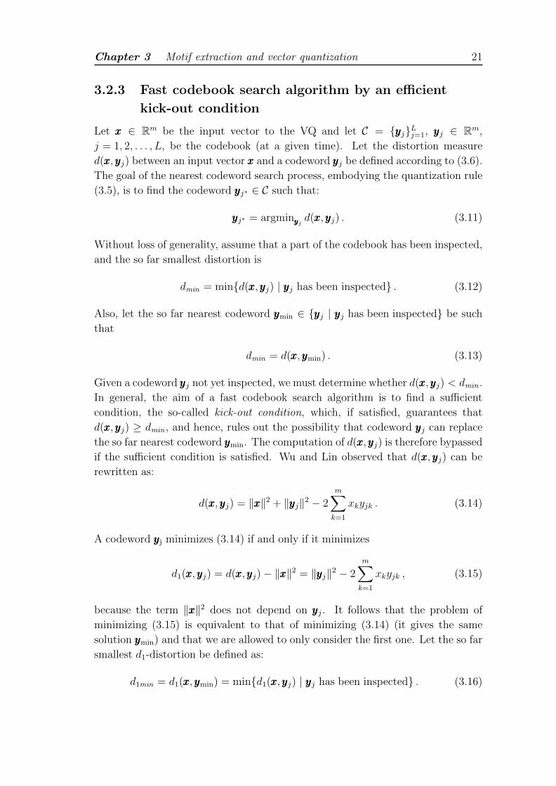
3.2.3 Fast codebook search algorithm by an efficient
kick-out condition
Let xxx ∈ Rm be the input vector to the VQ and let C = {yyyj}Lj=1, yyyj ∈ Rm,
j = 1, 2, . . . , L, be the codebook (at a given time). Let the distortion measure
d(xxx,yyyj) between an input vector xxx and a codeword yyyj be defined according to (3.6).
The goal of the nearest codeword search process, embodying the quantization rule
(3.5), is to find the codeword yyyj∗ ∈ C such that:
yyyj∗ = argminyyyj d(xxx,yyyj) . (3.11)
Without loss of generality, assume that a part of the codebook has been inspected,
and the so far smallest distortion is
dmin = min{d(xxx,yyyj) | yyyj has been inspected} . (3.12)
Also, let the so far nearest codeword yyymin ∈ {yyyj | yyyj has been inspected} be such
that
dmin = d(xxx,yyymin) . (3.13)
Given a codeword yyyj not yet inspected, we must determine whether d(xxx,yyyj) < dmin .
In general, the aim of a fast codebook search algorithm is to find a sufficient
condition, the so-called kick-out condition, which, if satisfied, guarantees that
d(xxx,yyyj) ≥ dmin , and hence, rules out the possibility that codeword yyyj can replace
the so far nearest codeword yyymin. The computation of d(xxx,yyyj) is therefore bypassed
if the sufficient condition is satisfied. Wu and Lin observed that d(xxx,yyyj) can be
rewritten as:
d(xxx,yyyj) = ‖xxx‖2 + ‖yyyj‖2 − 2m∑k=1
xkyjk . (3.14)
A codeword yyyj minimizes (3.14) if and only if it minimizes
d1(xxx,yyyj) = d(xxx,yyyj)− ‖xxx‖2 = ‖yyyj‖2 − 2m∑k=1
xkyjk , (3.15)
because the term ‖xxx‖2 does not depend on yyyj. It follows that the problem of
minimizing (3.15) is equivalent to that of minimizing (3.14) (it gives the same
solution yyymin) and that we are allowed to only consider the first one. Let the so far
smallest d1-distortion be defined as:
d1min = d1(xxx,yyymin) = min{d1(xxx,yyyj) | yyyj has been inspected} . (3.16)

Chapter 3 Motif extraction and vector quantization 22
Note that
d1(xxx,yyyj) ≥ ‖yyyj‖2 − 2‖xxx‖‖yyyj‖ = ‖yyyj‖(‖yyyj‖ − 2‖xxx‖) (3.17)
is always true, due to the Cauchy-Schwarz inequality. As a result, if a codeword yyyjsatisfies
‖yyyj‖(‖yyyj‖ − 2‖xxx‖) ≥ d1min , (3.18)
then d1(xxx,yyyj) ≥ d1min is guaranteed, and hence, yyyj should be kicked out because
it cannot be closer to xxx than yyymin is. For the input vector xxx, the computation of
‖yyyj‖(‖yyyj‖ − 2‖xxx‖) is quite simple, because the determination of {‖yyyj‖}Lj=1 can be
done in advance.
The complete algorithm by Wu and Lin is given in the following.
Algorithm 1 (Fast codebook search algorithm by an efficient
kick-out condition).
1. Initialization. Evaluate ‖yyyj‖ =√∑m
k=1 y2jk for every codeword in the code-
book C = {yyyj}Lj=1. Sort C so that ‖yyy1‖ ≤ ‖yyy2‖ ≤ . . . ≤ ‖yyyL‖.
2. Read an input vector xxx which is not encoded yet.
3. Evaluate 2‖xxx‖.
4. Choose a yyy(guess)min ∈ C and let
yyymin = yyy(guess)min , (3.19)
d1min = d1(xxx,yyymin) = d1(xxx,yyy(guess)min ) , (3.20)
R ={yyyj ∈ C | yyyj 6= yyy
(guess)min
}. (3.21)
5. a) If R = ∅, go to 6.
b) Pick a yyyj from R.
c) If
‖yyyj‖(‖yyyj‖ − 2‖xxx‖) ≥ d1min , (3.22)
then
i. if ‖yyyj‖ ≥ ‖xxx‖, then delete from R all yyyh such that h ≥ j and go to
5a);
ii. else delete from R all yyyh such that h ≤ j and go to 5a).
d) Evaluate d1(xxx,yyyj); delete yyyj from R; if d1(xxx,yyyj) ≥ d1min , then go to 5a).

Chapter 3 Motif extraction and vector quantization 23
e) Update the so far minimum distortion and the so far nearest codeword
(d1min = d1(xxx,yyyj), yyymin = yyyj) and go to 5a).
6. Return yyymin as the codeword minimizing (3.15) and hence (3.14).
7. Go to 2.
In step 1, I use the quicksort algorithm to sort the codewords in C. Indeed, the
quicksort algorithm is an efficient sorting algorithm commonly adopted in the sci-
entific community [34]. Mathematical analysis of quicksort shows that, on average,
the algorithm takes O(L logL) comparisons to sort L items. In the worst case, it
makes O(L2) comparisons, though this behavior is rare. When some optimizations
are taken into account during implementation (e.g., using insertion sort on small
arrays and choosing the pivot as the median of an array) it can be about two or
three times faster than its main competitors, mergesort and heapsort. In step 4
and 5b) I randomly choose a codeword in C and R, respectively. Note that the
timesaving is obtained through the check done in step 5c), which allows to skip
step 5e) and the time consuming step 5d) if condition (3.22) is satisfied. Note also
that in steps 5c-i) and 5c-ii) not only yyyj is kicked out but also all the codewords
yyyh ∈ R such that:
‖yyyh‖(‖yyyh‖ − 2‖xxx‖) ≥ ‖yyyj‖(‖yyyj‖ − 2‖xxx‖) ≥ d1min . (3.23)
To see why (3.23) is true, just note that the function c(t) = t(t− 2‖xxx‖) of variable
t is a parabola with its absolute minimum at t = ‖xxx‖. Moreover, note that the
problem of finding the codeword yyyj minimizing the Euclidean distance for a given
input vector xxx is equivalent to the problem of finding the codeword yyyj minimizing
the squared Euclidean distance (3.6). It follows that in my work, where I consider
the Euclidean distance (see Chapter 6), I am allowed to utilize the fast codebook
search algorithm just described.
Chapter 4
An overview of
artificial neural networks
4.1 What is an artificial neural network?
Artificial neural networks, also known as artificial neural nets, or ANNs for short,
represent one of the most promising computational tools in the artificial intelligence
research area. ANNs can be defined as massively parallel distributed processors
made up of a number of interlinked simple processing units, referred to as neurons,
that are able to store experiential knowledge from the surrounding environment
through a learning (or training) process and make the acquired knowledge available
for use [35]. The procedure used to perform the learning process is called a learning
algorithm and its function consists in tuning the interneuron connection strengths,
known as synaptic weights, in an orderly fashion, according to the data given as
input to the network. As a result, the acquired knowledge is encapsulated in the
synaptic weights and can be exploited to fulfill a particular assignment of interest.
Successful learning can result in ANNs that perform tasks such as predicting an
output value, classifying an object, approximating a function, recognizing a pattern
in multifactorial data, and completing a known pattern. Many works based on the
manifold abilities of ANNs can be found in the literature. For example, in [36]
the authors exploit ANNs to appropriately classify remotely sensed data; in [37]
the capability to uniformly approximate continuous functions on compact metric
spaces is proved for simple neural networks satisfying a few necessary conditions;
in [38] the cooperation of two ANNs is used for human face recognition and in [39]
a novel approach is proposed for speech recognition.
Work on ANNs have been motivated right from its inception by the recognition
that biological neural networks, in particular the human brain, compute in an en-
tirely different way from the conventional digital computer. The brain is a highly
complex, nonlinear and massively parallel information-processing system. It has
the capability to organize its structural constituents, the neurons, so as to perform
24
Chapter 4 An overview of artificial neural networks 25
certain computations (e.g., pattern recognition, perception, and motor control)
many times faster than the fastest digital computer in existence today. Consider,
for example, human vision. The brain routinely accomplishes perceptual recog-
nition tasks (e.g., recognizing a familiar face embedded in an unfamiliar scene) in
approximatively 100−200 ms, whereas tasks of much lesser complexity take a great
deal longer on a powerful computer. While in a silicon chip events happen in the
nanosecond range, neural events happen in the millisecond range. However, the
brain makes up for the relatively slow rate of operation by having a truly staggering
number of neurons with massive interconnections between them. It is estimated
that there are approximatively 10 billion neurons in the human cortex1, and 60
trillion connections. The key feature of the brain, which makes it an enourmously
efficient structure, is represented by its plasticity [40, 41], i.e., the ability to adapt
the neural connections (i.e., create new connections and modify the existing ones)
to the surrounding environment and then supply the information needed to interact
with it. The ANN, which is usually implemented by using electronic components
or simulated in software on a digital computer, is an adaptive machine designed
to model the way in which the brain works. Its computing power derives from its
parallel distributed structure and its ability to learn and therefore generalize, i.e.,
produce reasonable outputs for inputs not encountered during training. These in-
formation processing capabilities makes it possible for neural networks to find good
solutions to complex problems. Nevertheless, in practice, neural networks cannot
provide the solution by working individually but need to be integrated into a con-
sistent system engineering approach. Specifically, a complex problem of interest
is decomposed into a number of relatively simple tasks, and neural networks are
assigned a subset of the tasks that matches their inherent abilities.
4.2 Model of an artificial neuron
The fundamental information-processing unit of an ANN is the neuron, whose
model is directly inspired by its biological counterpart. In order to let the reader
appreciate the analogy, I will briefly describe the structure and functioning of a
biological neuron first. The model of an artificial neuron will follow.
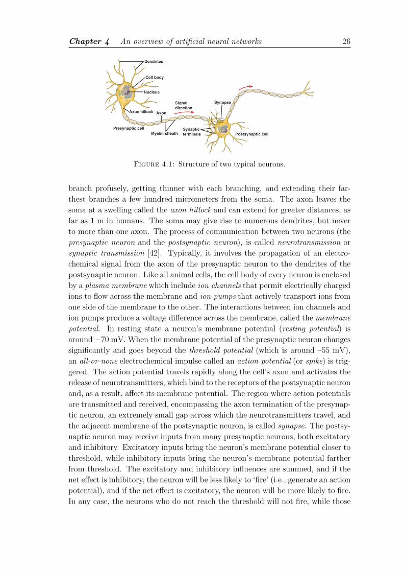
Neurons are the core components of the brain and spinal cord of the central
nervous system (CNS), and of the ganglia of the peripheral nervous system (PNS).
They are electrically excitable cells that process and transmit information through
electrochemical signals. A typical neuron consists of a cell body (or soma), den-
drites, and an axon, as illustrated in Figure 4.1. The soma is usually compact;
the axon and dendrites are filaments that extrude from it. Dendrites typically
1The cerebral cortex is the brain’s outer layer of neural tissue in humans and other mam-mals. It plays a fundamental role in memory, attention, perception, thought, language, andconsciousness.
Chapter 4 An overview of artificial neural networks 26
Figure 4.1: Structure of two typical neurons.
branch profusely, getting thinner with each branching, and extending their far-
thest branches a few hundred micrometers from the soma. The axon leaves the
soma at a swelling called the axon hillock and can extend for greater distances, as
far as 1 m in humans. The soma may give rise to numerous dendrites, but never
to more than one axon. The process of communication between two neurons (the
presynaptic neuron and the postsynaptic neuron), is called neurotransmission or
synaptic transmission [42]. Typically, it involves the propagation of an electro-
chemical signal from the axon of the presynaptic neuron to the dendrites of the
postsynaptic neuron. Like all animal cells, the cell body of every neuron is enclosed
by a plasma membrane which include ion channels that permit electrically charged
ions to flow across the membrane and ion pumps that actively transport ions from
one side of the membrane to the other. The interactions between ion channels and
ion pumps produce a voltage difference across the membrane, called the membrane
potential. In resting state a neuron’s membrane potential (resting potential) is
around −70 mV. When the membrane potential of the presynaptic neuron changes
significantly and goes beyond the threshold potential (which is around –55 mV),
an all-or-none electrochemical impulse called an action potential (or spike) is trig-
gered. The action potential travels rapidly along the cell’s axon and activates the
release of neurotransmitters, which bind to the receptors of the postsynaptic neuron
and, as a result, affect its membrane potential. The region where action potentials
are transmitted and received, encompassing the axon termination of the presynap-
tic neuron, an extremely small gap across which the neurotransmitters travel, and
the adjacent membrane of the postsynaptic neuron, is called synapse. The postsy-
naptic neuron may receive inputs from many presynaptic neurons, both excitatory
and inhibitory. Excitatory inputs bring the neuron’s membrane potential closer to
threshold, while inhibitory inputs bring the neuron’s membrane potential farther
from threshold. The excitatory and inhibitory influences are summed, and if the
net effect is inhibitory, the neuron will be less likely to ‘fire’ (i.e., generate an action
potential), and if the net effect is excitatory, the neuron will be more likely to fire.
In any case, the neurons who do not reach the threshold will not fire, while those
Chapter 4 An overview of artificial neural networks 27
Figure 4.2: Model of an artificial neuron.
that do must fire. This is the reason why the action potential is an ‘all-or-none’
event.
Let us now focus on ANNs. The model of an artificial neuron is reported in
Figure 4.2. Three basic elements of the neuron model can be identified:
• A set of synapses, or connecting links, each of which is characterized by a
weight or strength of its own. Specifically, a signal xk at the input of synapse
k connected to neuron j is multiplied by the synaptic weightwjk. The synaptic
weight of an artificial neuron may lie in a range that includes negative as well
as positive values.
• An adder (or linear combiner) for summing the input signals, weighted by
the respective synaptic weights of the neuron.
• An activation function (or squashing function) that limits the permissible
amplitude range of the output signal to some finite value.
The neural model in Figure 4.2 also includes an externally applied bias2, denoted
by bj. The bias bj has the effect of increasing or lowering the net input of the
activation function, depending on whether it is positive or negative, respectively.
In mathematical terms, the neuron j depicted in Figure 4.2 is described by the
pair of equations:
uj =m∑k=1
wjkxk (4.1)
and
yj = φ(uj + bj) , (4.2)
2The presence of the bias is not mandatory in neural models. It has been shown here for thesake of completeness.

Chapter 4 An overview of artificial neural networks 28
where x1, x2, . . . , xm are the input signals; wj1, wj2, . . . , wjm are the respective
synaptic weights of neuron j; uj (not shown in Figure 4.2) is the linear combiner
output due to the input signals; bj is the bias; φ(·) is the activation function; yjis the output signal of the neuron. The quantity vj = uj + bj is referred to as the
induced local field, or activation potential, of neuron j. Correspondingly, (4.2) may
be reformulated as yj = φ(vj).
There exist two basic types of activation functions:
• The threshold function (or Heaviside function), given by:
φ(v) =
{1, if v ≥ 0
0, if v < 0 .(4.3)
In neural computation, a neuron which uses the threshold function is referred
to as the McCulloch–Pitts model, in recognition of the pioneering work done
by McCulloch, a neuroscientist, and Pitts, a logician, who developed the first
conceptual model of an artificial neural network in 1943 [43]. In this model,
the output yj of a neuron takes on the value of 1 if the induced local field vj of
that neuron is nonnegative, and 0 otherwise. This statement describes the all-
or-none property of the McCulloch–Pitts model, which has been formulated
in accordance to the ‘all-or-none’ behavior of the action potential in biological
neurotransmission.
• The sigmoid function, whose graph is ‘S’-shaped and which is by far the
most common form of activation function used in the construction of neural
networks. An example of the sigmoid function is the logistic function, defined
by
φ(v) =1
1 + e−av, (4.4)
where a is the slope parameter. In the limit, as the slope parameter approaches
infinity, the sigmoid function becomes simply a threshold function. While a
threshold function assumes the value of 0 or 1, a sigmoid function assumes a
continuous range of values from 0 to 1. Note also that the sigmoid function
is differentiable, whereas the threshold function is not.
4.3 Network architectures
The manner in which the neurons are structured, i.e., the network architecture,
is intimately linked with the learning algorithm used to train the network. We
may therefore speak of learning algorithms used in the design of neural networks
as being structured. Three fundamentally different classes of network architectures
are identified:
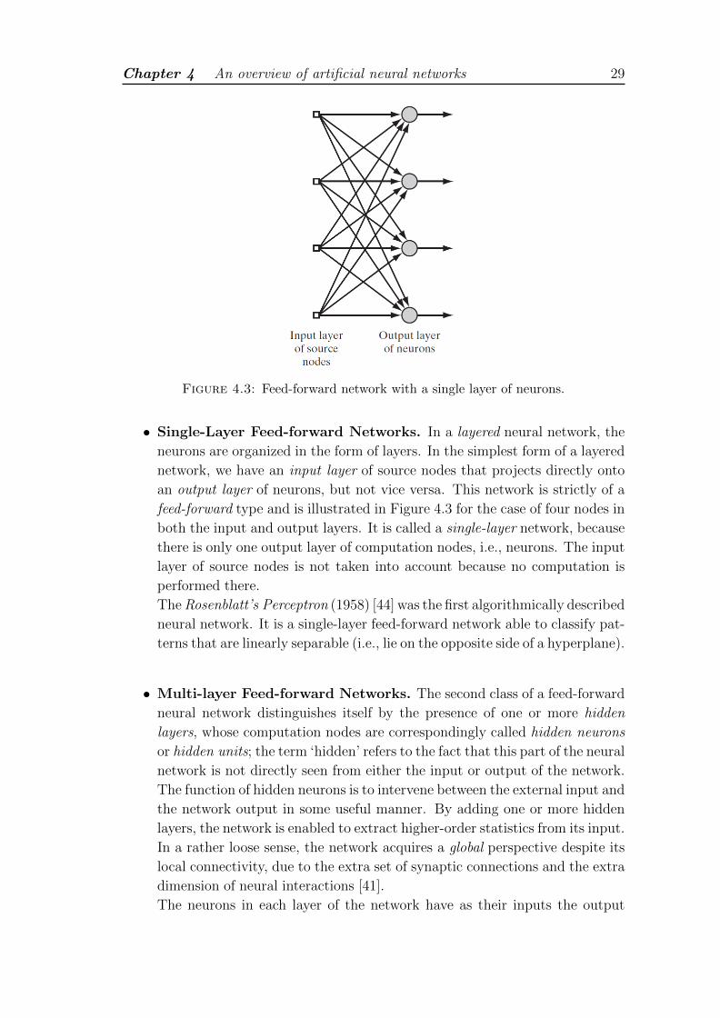
Chapter 4 An overview of artificial neural networks 29
Figure 4.3: Feed-forward network with a single layer of neurons.
• Single-Layer Feed-forward Networks. In a layered neural network, the
neurons are organized in the form of layers. In the simplest form of a layered
network, we have an input layer of source nodes that projects directly onto
an output layer of neurons, but not vice versa. This network is strictly of a
feed-forward type and is illustrated in Figure 4.3 for the case of four nodes in
both the input and output layers. It is called a single-layer network, because
there is only one output layer of computation nodes, i.e., neurons. The input
layer of source nodes is not taken into account because no computation is
performed there.
The Rosenblatt’s Perceptron (1958) [44] was the first algorithmically described
neural network. It is a single-layer feed-forward network able to classify pat-
terns that are linearly separable (i.e., lie on the opposite side of a hyperplane).
• Multi-layer Feed-forward Networks. The second class of a feed-forward
neural network distinguishes itself by the presence of one or more hidden
layers, whose computation nodes are correspondingly called hidden neurons
or hidden units; the term ‘hidden’ refers to the fact that this part of the neural
network is not directly seen from either the input or output of the network.
The function of hidden neurons is to intervene between the external input and
the network output in some useful manner. By adding one or more hidden
layers, the network is enabled to extract higher-order statistics from its input.
In a rather loose sense, the network acquires a global perspective despite its
local connectivity, due to the extra set of synaptic connections and the extra
dimension of neural interactions [41].
The neurons in each layer of the network have as their inputs the output
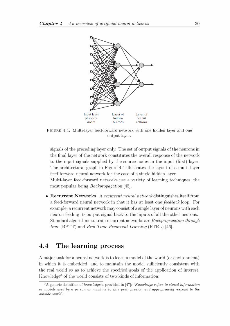
Chapter 4 An overview of artificial neural networks 30
Figure 4.4: Multi-layer feed-forward network with one hidden layer and oneoutput layer.
signals of the preceding layer only. The set of output signals of the neurons in
the final layer of the network constitutes the overall response of the network
to the input signals supplied by the source nodes in the input (first) layer.
The architectural graph in Figure 4.4 illustrates the layout of a multi-layer
feed-forward neural network for the case of a single hidden layer.
Multi-layer feed-forward networks use a variety of learning techniques, the
most popular being Backpropagation [45].
• Recurrent Networks. A recurrent neural network distinguishes itself from
a feed-forward neural network in that it has at least one feedback loop. For
example, a recurrent network may consist of a single layer of neurons with each
neuron feeding its output signal back to the inputs of all the other neurons.
Standard algorithms to train recurrent networks are Backpropagation through
time (BPTT) and Real-Time Recurrent Learning (RTRL) [46].
4.4 The learning process
A major task for a neural network is to learn a model of the world (or environment)
in which it is embedded, and to maintain the model sufficiently consistent with
the real world so as to achieve the specified goals of the application of interest.
Knowledge3 of the world consists of two kinds of information:
3A generic definition of knowledge is provided in [47]: ‘Knowledge refers to stored informationor models used by a person or machine to interpret, predict, and appropriately respond to theoutside world’.
Chapter 4 An overview of artificial neural networks 31
1. The known world state, represented by facts about what is and what has been
known; this form of knowledge is referred to as prior information.
2. Observations (measurements) of the world, obtained by means of sensors
designed to probe the environment, in which the neural network is supposed
to operate. Ordinarily, these observations are inherently noisy, being subject
to errors due to sensor noise and system imperfections.
It is the second kind of information that shall be used during the learning process.
Indeed, the observations of the world provide the examples used to train the neural
network. Such examples can be labeled or unlabeled. In labeled examples, each
example representing an input signal is paired with a corresponding desired response
(i.e., target output). On the other hand, unlabeled examples consist of different
realizations of the input signal all by itself. In any event, a set of examples, labeled
or otherwise, is referred to as the training set.
The learning process aims at acquiring the knowledge about the environment
as it is embodied by the training set and at providing a representation of such
knowledge by opportunely modifying the values taken on by the free parameters
(i.e., synaptic weights and biases) of the network. The knowledge representation
holds the key to the network performance. Since it heavily depends on the specific
architecture and learning process, the choice of these latter two constitute the very
design of the ANN.
In a broad sense, we may categorize the learning processes through which neural
networks function into two classes:
• Supervised learning (or learning with a teacher). Supervised learning
uses a training set of labeled examples and enables the ANN to learn com-
plicated input-output mappings. The learning process adjusts the network
parameters under the combined influence of the examples and the error sig-
nal, which is defined as the difference between the desired response and the
actual response of the network. This adjustment is carried out iteratively
in a step-by-step fashion with the aim of minimizing the error signal in ac-
cordance with an appropriate statistical criterion. The training continues
until the network reaches a steady state where there are no further significant
changes in the synaptic weights. When this condition is reached, the network
should be able to generalize when applied to signals not seen during training.
Supervised learning can be employed for pattern classification tasks, where
the requirement is to assign an input signal representing a physical object
or event to one of several prespecified categories. In this case, the desired
response is the category to which the corresponding input belongs.
• Unsupervised learning (or learning without a teacher). Unsupervised
learning uses a training set of unlabeled examples and allows the discovery
of significant patterns or features of the input data. In some cases, provision

Chapter 4 An overview of artificial neural networks 32
is made for a task-independent measure of the quality of representation that
the network is required to learn, and the free parameters of the network
are optimized with respect to that measure. For a specific task-independent
measure, once the network has become tuned to the statistical regularities
of the input data, it develops the ability to form internal representations for
encoding features of the input data.
In this work, I used the TASOM, an ANN based on unsupervised learning. In
order to fully clarify how its implementation (and that of the SOM, from which
the TASOM derives) can be accomplished, I dedicate the following section to the
principles of unsupervised learning. Then, in Chapter 5, I proceed with the pre-
sentation of the SOM and TASOM architectures and of the corresponding learning
algorithms.
4.5 Unsupervised learning
The goal of unsupervised learning, also called self-organized learning, is to fit a
model to a set of unlabeled input data in such a way that the underlying structure
of the data is well represented. It is based on four principles [35]:
Principle 1. Self-amplification
The first principle of self-organization states that:
Modifications in the synaptic weights of a neuron tend to self-amplify
in accordance with Hebb’s postulate of learning, which is made possible
by synaptic plasticity.
Hebb’s postulate of learning is the oldest and most famous of all learning rules and
has been originally defined for a neurobiological context; it is named in honor of
the neuropsychologist Hebb. Hebb’s book The Organization of Behavior (1949)
asserts the following (p. 62):
When an axon of cell A is near enough to excite a cell B and repeatedly
or persistently takes part in firing it, some growth process or metabolic
changes take place in one or both cells such that A’s efficiency as one
of the cells firing B is increased.
Thus, if we define as the presynaptic signal the signal carried by the presynaptic
neuron (cell A) and as the postsynaptic signal the signal carried by the postsynaptic
neuron (cell B), we can say that the first principle of self-organization specify a
feedback mechanism, by means of which a strong synapse leads to the coincidence of
presynaptic and postsynaptic signals. In turn, the synapse is increased in strength
by such a coincidence. According to [48, 49], these requirements can be rephrased
as a two-part rule:

Chapter 4 An overview of artificial neural networks 33
1. If two neurons on either side of a synapse are activated simultaneously (i.e.,
synchronously), then the strength of that synapse is selectively increased.
2. If two neurons on either side of a synapse are activated asynchronolusly, then
that synapse is selectively weakened or eliminated.
Such a synapse is called a Hebbian synapse, although the original Hebbian rule did
not contain part 2. A more sophisticated definition can be found in [50], where a
Hebbian synapse is described as a synapse that uses a time-dependent, highly local,
and strongly interactive mechanism to increase synaptic efficiency as a function
of the correlation between the presynaptic and postsynaptic activities. Hence, the
following four key mechanisms characterize Hebbian learning and, as a consequence,
the self-amplification principle of self-organization:
1. Time-dependent mechanism. This mechanism refers to the fact that the
modifications in a Hebbian synapse depend on the exact time of occurrence
of the presynaptic and postsynaptic signals.
2. Local mechanism. By its very nature, a synapse is the transmission site where
information-bearing signals (representing ongoing activity in the presynaptic
and postsynaptic units) are in spatiotemporal contiguity. This locally avail-
able information is used by a Hebbian synapse to produce a local synaptic
modification that is input specific.
3. Interactive mechanism. The occurrence of a change in a Hebbian synapse
depends on signals on both sides of the synapse. That is, the Hebbian form of
learning depends on ‘true interaction’ between presynaptic and postsynaptic
signals in the sense that we cannot make a prediction from either one of these
two activities by itself.
4. Conjunctional or correlational mechanism. One interpretation of Hebb’s pos-
tulate of learning is that the condition for a change in synaptic efficiency is
the conjunction of presynaptic and postsynaptic signals. Thus, according to
this interpretation, the cooccurrence of presynaptic and postsynaptic signals
(within a short interval of time) is sufficient to produce the synaptic modi-
fication. It is for this reason that a Hebbian synapse is sometimes referred
to as a conjunctional synapse. For another interpretation of Hebb’s postu-
late of learning, we may think of the interactive mechanism characterizing a
Hebbian synapse in statistical terms. In particular, the correlation over time
between presynaptic and postsynaptic signals is viewed as being responsible
for a synaptic change. Accordingly, a Hebbian synapse is also referred to as
a correlational synapse. Correlation is indeed the basis of learning [51].
To formulate the Hebbian learning in mathematical terms, consider a synaptic
weight wjk of neuron j with presynaptic and postsynaptic signals denoted by xk
Chapter 4 An overview of artificial neural networks 34
and yj, respectively. The adjustment applied to the synaptic weight wjk at time-
step n is expressed in the general form as
∆wjk(n) = wjk(n+ 1)− wjk(n) = f(yj(n), xk(n)) , (4.5)
where f(·) is a function of both postsynaptic and presynaptic signals. The formula
(4.5) admits many forms, all of which qualify as Hebbian. The simplest form of
Hebbian learning is described by
∆wjk(n) = ηyj(n)xk(n) , (4.6)
where η is a positive constant that determines the rate of learning and is referred to
as the learning-rate. Equation (4.6) clearly emphasizes the correlational nature of a
Hebbian synapse. From this representation, we see that the repeated application of
the input signal (presynaptic activity) xj leads to an increase in yk and, therefore,
exponential growth that finally drives the synaptic connection into saturation. At
that point, no new information will be stored in the synapse, and selectivity is lost.
Some mechanism is therefore needed to stabilize the self-organized behavior of the
neuron, which is taken care of by the second principle.
Principle 2. Competition
This second principle of self-organization states the following:
The limitation of available resources, in one form or another, leads to
competition among the synapses of a single neuron or an assembly of
neurons, with the result that the most vigorously growing (i.e., fittest)
synapses or neurons, respectively, are selected at the expense of the
others.
This second principle is made possible by synaptic plasticity (i.e., adjustability of
a synaptic weight) and allows the network to stabilize. For a given single neuron,
for example, there must be competition among its synapses for limited resources
(e.g., energy) in such a way that the increase in strength of some synapses in the
neuron is compensated for by a decrease in strength in others. Accordingly, only
the ‘successful’ synapses can grow in strength, while the less successful synapses
tend to weaken and may eventually disappear altogether. One way to introduce
competition among the synapses of a neuron is to incorporate some form of normal-
ization in the learning rule for the adaptation of the synaptic weights. For example,
a modification of the Hebbian learning rule, called Oja’s rule [52], recasts (4.6) in
the new form
wjk(n+ 1) =wjk(n) + ηyj(n)xk(n)√∑mk=1(wjk(n) + ηyj(n)xk(n))2
, (4.7)
Chapter 4 An overview of artificial neural networks 35
where the summation in the denominator extends over the complete set of synapses
(with cardinality m) associated with the neuron j. Assuming that the parameter η
is small and that the neuron j acts as a linear combiner (i.e., the postsynaptic signal
yj(n) is given at any time-step n by the sum of its presynaptic signals xk(n), k =
1, . . . ,m, weighted by the corresponding synaptic weights wjk(n)), it can be proved
that (4.7) is equivalent to [35]
wjk(n+ 1) = wjk(n) + ηyj(n)(xk(n)− yj(n)wjk(n)) , (4.8)
where the term yj(n)xk(n) represents the usual Hebbian adaptation and therefore
accounts for the self-amplification effect dictated by Principle 1 of self-organization.
The negative term −yj(n)wjk(n) is responsible for stabilization in accordance with
Principle 2. It is related to a forgetting, or leakage term, that is frequently used
in learning rules, but with the difference that it becomes more pronounced with a
stronger postsynaptic signal yj(n).
At the network level, a competitive process may prevail by proceeding as fol-
lows [53]:
• To begin with, the neurons in the network are all the same, except for some
randomly distributed synaptic weights; hence, the neurons respond differently
to a given set of input patterns.
• A specific limit is imposed on the ‘strength’ (e.g., the sum of synaptic weights)
of each neuron in the network.
• The neurons compete with each other in accordance with a prescribed rule
for the right to respond to a given subset of inputs; consequently, only one
output neuron, or one neuron per group, is active at a time. The neuron that
wins the competition is called a winner-takes-all neuron (or simply winning)
neuron.
Through this competitive-learning process, the individual neurons of the network
assume the role of feature detectors for different classes of input patterns. Whereas
in Hebbian learning several output neurons of a neural network may be active
simultaneously, in competitive learning only a single output neuron, or one output
neuron per group, is active at any one time. It is this characteristic of competitive
learning that makes it highly suited to discovering statistically salient features
which could be used to classify a set of input patterns.
Principle 3. Cooperation
This third principle of self-organization states the following:
Modifications in synaptic weights at the neural level and in neurons at
the network level tend to cooperate with each other.
Chapter 4 An overview of artificial neural networks 36
The cooperation may arise because of synaptic plasticity or because of simultane-
ous stimulation of presynaptic neurons brought on by the existence of the right
conditions in the external environment. Consider first the case of a single neuron:
a single synapse on its own cannot efficiently produce favorable events. Rather,
there has to be cooperation among the neuron’s synapses, making it possible to
carry coincident signals strong enough to activate that neuron. At the network
level, cooperation may take place through lateral interaction among a group of
excited neurons. In particular, a firing neuron tends to excite the neurons in its
immediate neighborhood more so than those farther away from it. Over the course
of time, we typically find that a cooperative system evolves through a sequence of
small changes from one configuration to another, until an equilibrium condition is
established. It is also important to note that in a self-organizing system that in-
volves both competition and cooperation, competition always precedes cooperation.
Principle 3. Structural Information
The fourth, and last, principle of self-organization states the following:
The underlying order and structure that exist in an input signal rep-
resent redundant information, which is acquired by a self-organizing
system in the form of knowledge.
Structural information contained in the input data is therefore a prerequisite to
self-organized learning. It is also noteworthy that whereas self-amplification, com-
petition, and cooperation are processes that are carried out within a neuron or a
neural network, structural information, or redundancy, is an inherent characteristic
of the input signal. Consider, for example, a voice or video signal. When such a sig-
nal is sampled at a high rate, the resulting sampled signal is correspondingly found
to exhibit a higher degree of correlation between adjacent samples. The meaning
of this high correlation is that, on average, the signal does not change rapidly from
one sample to the next, which, in turn, means that the signal contains structured, or
redundant, information. In other words, correlation is synonymous with structure
and redundancy. To appreciate the importance of structure, suppose that all the
redundant information contained in a signal is completely removed. What is then
left is a completely non-redundant signal that is unpredictable and may therefore
be indistinguishable from noise. Given this kind of an input, no self-organizing or
unsupervised-learning system can function.
Chapter 5
The self-organizing maps:
SOM and TASOM
The self-organizing map (SOM) is a kind of ANN based on unsupervised learning
which was invented by the Finnish professor Teuvo Kohonen in the 1980. It has
the characteristic property of providing a structured representation of the input
data distribution by the neurons’ synaptic weights as prototypes [54]. Typically
the self-organizing map has a single-layer feed-forward architecture (see Section
4.3) where neurons are placed at the nodes of a lattice that is usually one or two di-
mensional. Higher dimensional maps are also possible but not as common. During
the unsupervised learning process the neurons become selectively tuned to vari-
ous input patterns by competing among themselves. The synaptic weights of the
neurons that win the competitions are modified according to an adaptation rule
that tends to order the neurons with respect to each other, developing a significant
coordinate system for different input features over the lattice. A SOM therefore
creates a topographic map of the input data space, in which the spatial locations
or coordinates of the neurons in the lattice correspond to a particular domain or
intrinsic statistical feature of the input data, without any prior knowledge on the
input distribution - hence, the name self-organizing map.
The definition of a SOM as a neural model is justified by the fact that in higher
animals different sensory inputs, such as tactile, visual, and acoustic, are mapped
onto different areas of the cerebral cortex in a topologically ordered manner [55].
Thus the learning results achieved with a SOM seem very natural, at least indicating
that the adaptive processes at work in the map may be similar to those encountered
in the brain.
5.1 The SOM algorithm
The map formation is carried out through the learning process, whose original
version was developed by Kohonen during a long series of computer experiments
37
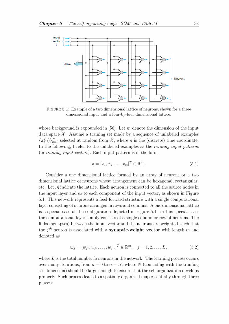
Chapter 5 The self-organizing maps: SOM and TASOM 38
Figure 5.1: Example of a two dimensional lattice of neurons, shown for a threedimensional input and a four-by-four dimensional lattice.
whose background is expounded in [56]. Let m denote the dimension of the input
data space X . Assume a training set made by a sequence of unlabeled examples
{xxx(n)}Nn=0 selected at random from X , where n is the (discrete) time coordinate.
In the following, I refer to the unlabeled examples as the training input patterns
(or training input vectors). Each input pattern is of the form
xxx = [x1, x2, . . . , xm]T ∈ Rm . (5.1)
Consider a one dimensional lattice formed by an array of neurons or a two
dimensional lattice of neurons whose arrangement can be hexagonal, rectangular,
etc. Let A indicate the lattice. Each neuron is connected to all the source nodes in
the input layer and so to each component of the input vector, as shown in Figure
5.1. This network represents a feed-forward structure with a single computational
layer consisting of neurons arranged in rows and columns. A one dimensional lattice
is a special case of the configuration depicted in Figure 5.1: in this special case,
the computational layer simply consists of a single column or row of neurons. The
links (synapses) between the input vector and the neurons are weighted, such that
the jth neuron is associated with a synaptic-weight vector with length m and
denoted as
wwwj = [wj1, wj2, . . . , wjm]T ∈ Rm, j = 1, 2, . . . , L , (5.2)
where L is the total number fo neurons in the network. The learning process occurs
over many iterations, from n = 0 to n = N , where N (coinciding with the training
set dimension) should be large enough to ensure that the self organization develops
properly. Such process leads to a spatially organized map essentially through three
phases:
Chapter 5 The self-organizing maps: SOM and TASOM 39
1. Competition. For each input pattern, the neurons in the network compute
their respective values of a discriminant function. This discriminant function
provides the basis for competition among the neurons. The particular neuron
with the minimum value of the discriminant function is declared winner of
the competition.
2. Cooperation. The winning neuron determines the spatial location of a topo-
logical neighborhood of excited neurons, thereby providing the basis for co-
operation among such neighboring neurons.
3. Synaptic Adaptation. This last mechanism enables the excited neurons to
reduce the value of their discriminant functions in relation to the input pat-
tern through suitable adjustments applied to their synaptic weights. The
adjustments made are such that the response of the winning neuron to the
subsequent application of a similar input pattern is enhanced.
The first two phases are in accordance with two of the four principles of self-
organization described in Section 4.5. Synaptic adaptation embodies the principle
of self-amplification by using a modified form of Hebbian learning. As explained in
Section 4.5, the presence of redundancy in the input data, though not mentioned
explicitly in describing the SOM algorithm, is essential for learning, since it pro-
vides knowledge about the underlying structure of the input patterns. Detailed
descriptions of the processes of competition, cooperation, and synaptic adaptation
are presented in what follows.
5.1.1 Competition
At each iteration a training input pattern from {xxx(n)}Nn=0 is presented to the net-
work and the neurons compete among themselves to be selected as the winning
neuron (also called the best matching neuron). To determine which neuron is going
to be selected, the input vector is compared with the synaptic-weight vectors of
the neurons. Only the neuron whose synaptic-weight vector most closely matches
the current input vector according to a given distance measure (that I chose equal
to the Euclidean distance, as it is in typical applications) dominates. If we use the
index i(xxx) to identify the neuron that best matches the input vector xxx(n), we may
then determine i(xxx) by applying the following condition, which sums up the essence
of the competition process among the neurons:
i(xxx) = argminj ‖xxx(n)−wwwj(n)‖ , j = 1, 2, . . . , L . (5.3)
5.1.2 Cooperation
The winning neuron locates the center of a topological neighborhood of cooperating
neurons. Indeed, a crucial requirement for the formation of ordered maps is that
Chapter 5 The self-organizing maps: SOM and TASOM 40
the neurons involved in the learning are not affected independently of each other,
but as topologically related subsets, on each of which a similar kind of correction
is imposed. In biophysically inspired neural network models, correlated learning
by spatially neighboring neurons can be implemented using various kinds of lateral
feedback connection and other lateral interactions. In the SOM algorithm, lateral
interaction is directly enforced by defining the neighborhood function hji, which
introduces a topological neighborhood centered on the winning neuron i(xxx) and
encompassing a set of excited (cooperating) neurons, a typical one of which is
denoted by j. The neighborhood function should decay smoothly with lateral
distance, according to the neurobiological evidence that a firing neuron tends to
excite the neurons in its immediate neighborhood more than those farther away
from it. If dji is the lateral distance between i(xxx) and neuron j, then hji has to
be symmetric about the maximum point defined by dji = 0 and its amplitude
has to decrease monotonically with increasing lateral distance dji, decaying to zero
for dji → ∞. A good choice of hji is the Gaussian function, which is translation
invariant:
hji = exp
(−d2ji2σ2
), (5.4)
where the parameter σ is the width of the topological neighborhood (referred to
as neighborhood width) that measures the degree to which excited neurons in the
vicinity of the winning neuron participate in the learning process.
Another requirement that hji has to satisfy is to be shrinking with time, which
can be achieved by making σ decrease with time. Actually, it turned out to be ad-
vantageous for the map to stabilize to let the radius of the topological neighborhood
be very wide in the beginning and shrink monotonically as time goes by. The ex-
planation for this is that a wide initial topological neighborhood, corresponding to
a coarse spatial resolution in the learning process, first induces a rough global order
in the synaptic-weight vectors’ values, after which narrowing improves the spatial
resolution of the map without destroying the acquired global order. A popular
choice for the time dependence of σ is the exponential decay described by
σ(n) = σ0 exp
(− nτ1
), n = 0, 1, . . . (5.5)
where σ0 is the value of σ at the initialization of the SOM algorithm and τ1 is a
time constant to be chosen by the designer.
Correspondingly hji takes the time-varying form
hji(n) = exp
(−
d2ji2σ2(n)
), n = 0, 1, . . . (5.6)
with σ(n) defined in (5.5).
Chapter 5 The self-organizing maps: SOM and TASOM 41
5.1.3 Synaptic Adaptation
The last phase requires the synaptic-weight vector of the excited neurons to change
in relation to the input vector xxx(n). In Hebb’s postulate of learning, a synaptic
weight is increased with a simultaneous occurrence of presynaptic and postsynaptic
activities. For the type of unsupervised learning being considered here, however,
the Hebbian hypothesis in its basic form is unsatisfactory, since changes in con-
nectivities occur in one direction only, finally driving all the synaptic weights into
saturation, as seen in Sub-section 4.5. To overcome this problem, Kohonen modified
the Hebbian assumption by including a forgetting term that leads to the following
adaptation rule for the synaptic-weight vector wwwj(n) of neuron j at time n:
wwwj(n+ 1) = wwwj(n) + η(n)hji(n)(xxx(n)−wwwj(n)) . (5.7)
(5.7) has the effect of moving the synaptic-weight vector wwwi(xxx) of the winning neu-
ron i(xxx) (and to a lesser extent the synaptic-weight vectors of the neurons in its
topological neighborhood) toward the input vector xxx to more closely resemble the
data for the class the input vector is a member of. The algorithm therefore leads
to a topological ordering of the feature map in the input space in the sense that
neurons that are adjacent in the lattice will tend to have similar synaptic-weight
vectors. According to the principles of stochastic approximation, the learning-rate
η(n) should start at some initial value η0 and then decrease gradually with increas-
ing time n. This requirement can be satisfied by the following expression:
η(n) = η0 exp
(− nτ2
), n = 0, 1, . . . (5.8)
where τ2 is another time constant.
The adaptive process of the synaptic weights in the network, computed in ac-
cordance with Equation (5.7), may be decomposed into two phases: an ordering
phase, followed by a convergence phase. These two phases of the adaptive process
are described next:
1. Ordering phase. It is during this first phase that the topological ordering
of the weight vectors takes place. The ordering phase may take as many
as 1000 iterations of the SOM algorithm, and possibly even more. Careful
consideration must therefore be given to the choice of the learning-rate and
neighborhood function. The learning-rate η(n) should be initialized to a value
close to 0.1; thereafter it should decrease gradually, but remain above 0.01
(i.e., it should never be allowed to get to zero). The neighborhood function
hji(n) should initially include almost all neurons in the network centered on
the winning neuron and then slowly reduce to a small value of only a couple
of neighboring neurons around the winning neuron or to the winning neuron
by itself. Suitable values for the parameters in Equations (5.5) and (5.8), are
Chapter 5 The self-organizing maps: SOM and TASOM 42
thus the following:
τ1 =1000
log σ0
η0 = 0.1 (5.9)
τ2 = 1000,
where σ0, assuming the use of a two dimensional lattice of neurons, should
be set equal to the ‘radius’ of the lattice.
2. Convergence phase. This second phase of the adaptive process is needed
to fine-tune the feature map and therefore provide an accurate statistical
quantification of the input space. Moreover, the number of iterations needed
for convergence strongly depends on the dimensionality of the input space.
As a general rule, the number of iterations constituting the convergence phase
must be at least 500 times the number of neurons in the network. For good
statistical accuracy, the learning-rate η(n) should be maintained during the
convergence phase at a small value, on the order of 0.01. The neighborhood
function hji(n) should only contain the nearest neighbors of a winning neuron,
which may eventually reduce to one or zero neighboring neurons.
5.2 Summary of the SOM algorithm
There are three basic steps involved in the application of the algorithm after initial-
ization: sampling, similarity matching, and synaptic weights update. The algorithm
steps can be described as follows:
Algorithm 2 (SOM).
1. Initialization. Set n = 0 and for each neuron j in the lattice A pick small
random values for the initial synaptic-weight vectors wwwj(0).
2. Sampling. Let n be a generic time step. Consider a training input pattern
xxx(n).
3. Similarity matching. Find the best matching (winning) neuron i(xxx) at
time step n, i.e., the neuron that best represents xxx(n), by using the minimum-
distance criterion:
i(xxx) = argminj ‖xxx(n)−wwwj(n)‖, j = 1, 2, . . . , L , (5.10)
where ‖aaa−bbb‖ is the norm of the vector aaa−bbb and thus is equal to the Euclidean
distance between aaa and bbb.
Chapter 5 The self-organizing maps: SOM and TASOM 43
4. Synaptic weights update. Adjust the synaptic-weight vectors of all neu-
rons j ∈ A by using the update rule:
wwwj(n)← wwwj(n) + η(n)hji(n)(xxx(n)−wwwj(n)) , (5.11)
where η(n) is the learning-rate parameter at iteration n and hji(n) is the
neighborhood function centered on i(xxx) at iteration n.
5. Iteration. Set n ← n + 1 and continue with step 2 if n < N + 1, stop
otherwise.
5.3 Properties of the SOM
Starting from an initial state of disorder, the SOM algorithm gradually leads to a
topological representation of the input data space in the sense that adjacent neurons
in the lattice will tend to have similar synaptic-weight vectors and will correspond
to a particular class or feature of the input data. The final statistical accuracy
of the mapping depends on the number of iterations. As indicated in Sub-section
5.1.3, a rule of thumb to guarantee the convergence to an accurate map is that the
number of iterations must be at least N = 1000 + 500L where L is the number
of neurons [54]. Once the algorithm has terminated, a nonlinear transformation
ΦΦΦ : X → A called a feature map can be defined. Given an input vector xxx, ΦΦΦ(xxx)
corresponds to the best matching neuronwwwi(xxx) in the final map, where the index i(xxx)
is found according to the similarity matching step (5.10). The SOM capabilities lie
in ΦΦΦ(·)’s properties:
1. ΦΦΦ(·) provides a projection from the continuous high dimensional data space
X onto the low dimensional discrete neural space A, thus it provides dimen-
sionality reduction.
2. ΦΦΦ(·) provides a good approximation to the input data space X . Actually, the
SOM represents the continuous space X by finding a finite set of prototypes
wwwj ∈ A whose synaptic-weight vectors can be considered as representative of
all the input vectors xxx such that ΦΦΦ(xxx) = wwwj. In this perspective, the SOM
algorithm is a vector quantization algorithm.
3. ΦΦΦ(·) is topologically ordered in the sense that the spatial location of a neuron in
the lattice corresponds to a particular domain or feature of input patterns. In
other words, similar input patterns are clustered together and represented by
a specific neuron in the latticeA. Therefore, ΦΦΦ may be displayed as an elastic
net with the topology of a one or two dimensional lattice (as prescribed byA)
where nodes have synaptic-weight vectors’ components as coordinates in the
input space X and neighboring nodes are connected by lines, as illustrated in
Figure 5.2.
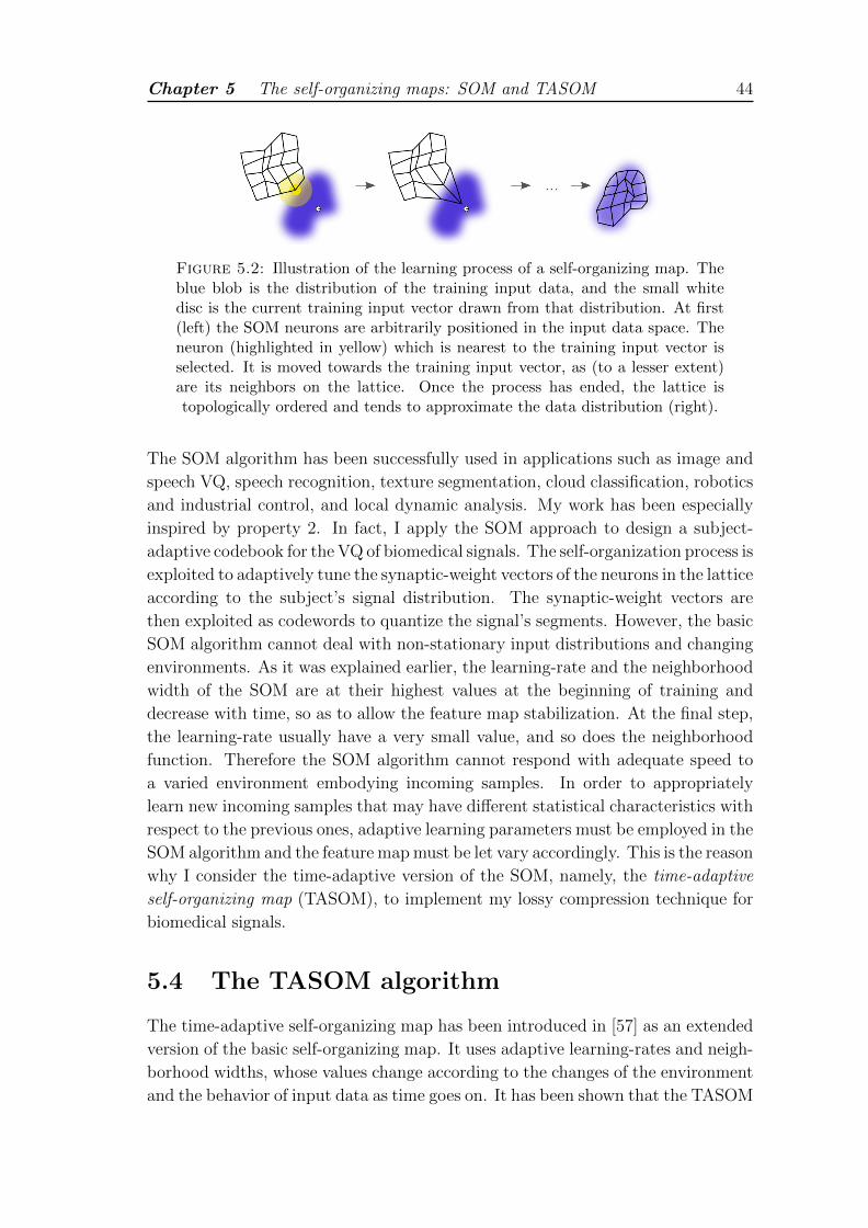
Chapter 5 The self-organizing maps: SOM and TASOM 44
Figure 5.2: Illustration of the learning process of a self-organizing map. Theblue blob is the distribution of the training input data, and the small whitedisc is the current training input vector drawn from that distribution. At first(left) the SOM neurons are arbitrarily positioned in the input data space. Theneuron (highlighted in yellow) which is nearest to the training input vector isselected. It is moved towards the training input vector, as (to a lesser extent)are its neighbors on the lattice. Once the process has ended, the lattice istopologically ordered and tends to approximate the data distribution (right).
The SOM algorithm has been successfully used in applications such as image and
speech VQ, speech recognition, texture segmentation, cloud classification, robotics
and industrial control, and local dynamic analysis. My work has been especially
inspired by property 2. In fact, I apply the SOM approach to design a subject-
adaptive codebook for the VQ of biomedical signals. The self-organization process is
exploited to adaptively tune the synaptic-weight vectors of the neurons in the lattice
according to the subject’s signal distribution. The synaptic-weight vectors are
then exploited as codewords to quantize the signal’s segments. However, the basic
SOM algorithm cannot deal with non-stationary input distributions and changing
environments. As it was explained earlier, the learning-rate and the neighborhood
width of the SOM are at their highest values at the beginning of training and
decrease with time, so as to allow the feature map stabilization. At the final step,
the learning-rate usually have a very small value, and so does the neighborhood
function. Therefore the SOM algorithm cannot respond with adequate speed to
a varied environment embodying incoming samples. In order to appropriately
learn new incoming samples that may have different statistical characteristics with
respect to the previous ones, adaptive learning parameters must be employed in the
SOM algorithm and the feature map must be let vary accordingly. This is the reason
why I consider the time-adaptive version of the SOM, namely, the time-adaptive
self-organizing map (TASOM), to implement my lossy compression technique for
biomedical signals.
5.4 The TASOM algorithm
The time-adaptive self-organizing map has been introduced in [57] as an extended
version of the basic self-organizing map. It uses adaptive learning-rates and neigh-
borhood widths, whose values change according to the changes of the environment
and the behavior of input data as time goes on. It has been shown that the TASOM
Chapter 5 The self-organizing maps: SOM and TASOM 45
works well both with stationary and non-stationary environments, preserving the
SOM properties. Examples of applications are adaptive shape representation and
adaptive segmentation, adaptive pattern classification, adaptive principal compo-
nent analysis, and automatic multilevel thresholding.
The TASOM structure does not differ from that of the SOM. However, every
neuron j, j = 1, 2, . . . , L, in the latticeA has its own learning-rate ηj and neighbor-
hood width σj, so as to allow for a continuous (potentially unlimited) training of the
synaptic-weight vectors. This feature enables the TASOM to be more flexible and
better approximate the input data space distribution as it evolves, adapting the
synaptic-weight vectors to the more recent input data if they substantially differ
from the previous one.
For a squared lattice with L = M2 neurons and input vectors with dimension
m the TASOM algorithm is specified as:
Algorithm 3 (TASOM).
1. Initialization. Set n = 0 and for each neuron j in the lattice A do the
following:
• Pick small random values for the initial synaptic-weight vectors wwwj(0).
• Set the initial learning-rate ηj(0) to a value close to one.
• Set the initial neighborhood width σj(0) so that the neighborhood func-
tion includes all the neurons in the map.
• Define the set NHj as the set of the immediate neighbors of neuron j.
Let α, αs, β, βs be constant parameters used to adapt the learning-rate and
the neighborhood width updating behavior. Initialize them to small values
in (0, 1). Define a scaling vector sss(0) = [s1(0), s2(0), . . . , sm(0)]T and initial-
ize its elements to small positive values. Define the variable (scaling value)
sv(0) = ‖sss(0)‖. sv(n) approximates the diameter of the input distribution to
help the TASOM to remain scaling invariant. Initialize two further param-
eters Ek(0), E2k(0) with some small positive random values. These, will be
used to update sss.
2. Sampling. Now, let n be a generic time step. Consider an input pattern
xxx(n) = [x1(n), . . . , xm(n)]T from the input data space.
3. Similarity matching. Find the winning neuron i(xxx) at time step n using
Eq. (5.3).
4. Scaling vector update. For k = 1, . . . ,m do
E2k(n)← E2k(n) + αs(x2k(n)− E2k(n)) , (5.12)
Ek(n)← Ek(n) + βs(xk(n)− Ek(n)) , (5.13)

Chapter 5 The self-organizing maps: SOM and TASOM 46
sk(n)←√
max((E2k(n)− Ek(n)2), 0) (5.14)
and adjust sv(n) as sv(n)← ‖sss(n)‖.
5. Neighborhood width update. Adjust the neighborhood width of the
winning neuron i(xxx) as
σi(n)← σi(n) + β
[g
(1
sg|NHi|∑j∈NHi
‖wwwi(n)−wwwj(n)‖s)− σi(n)
], (5.15)
where | · | returns the cardinality of a set. g(z) is used to normalize the
weight distances and I assume g(z) = (√
2M − 1)(z/(z + 1)). sg is a user set
parameter and the scaled norm is defined as ‖ · ‖s = ‖ · ‖/sv(n).
6. Learning-rate update. Adjust the learning-rate ηj(n) of every neuron
j ∈ A as:
ηj(n)← ηj(n) + α
[f
(1
sf‖xxx(n)−wwwj(n)‖s
)− ηj(n)
]. (5.16)
f(z) is used to normalize the distance between the synaptic-weight and input
vectors. Here, I use f(z) = z/(z + 1). sf is a user set parameter.
7. Synaptic weights update. Adjust the synaptic-weight vectors of all neu-
rons j ∈ A through the following rule
wwwj(n)← wwwj(n) + ηj(n)hji(n)(xxx(n)−wwwj(n)) , (5.17)
where index i stands for the winning neuron and Eq. (5.6) is used as the
neighborhood function.
8. Iteration. Set n← n+ 1 and continue with step 2.
By taking a closer look at the updating rules (5.16) and (5.15), we can better
understand why the TASOM is able to adapt to non-stationary environments. By
replacing the discrete time variable with its continuous counterpart, and assuming
that ∆t is a very small positive value, the learning-rate update of (5.16) may be
written as:
dηj(t)
dt= −αηj(t) + αf(‖xxx(t)−wwwj(t)‖f ) , (5.18)
where ‖xxx(t) − wwwj(t)‖f = ‖xxx(t) − wwwj(t)‖s/sf . If we assume that the changes of
‖xxx(t)−wwwj(t)‖f with time are much smaller than that of the learning-rate ηj(t), we
can solve the above non-homogeneous first-order differential equation as:
ηj(t) = ηj(0)e−αt + (1− e−αt)f(‖xxx(t)−wwwj(t)‖f ) , (5.19)
Chapter 5 The self-organizing maps: SOM and TASOM 47
where ηj(0) is the initial learning-rate of neuron j. The first term on the right-hand
side (RHS) of (5.19) decreases exponentially to zero as time goes to infinity, as
in the basic SOM. As for the second term on the RHS, function ‖xxx(t) − wwwj(t)‖fresembles a normalized error for neuron j. As time goes to infinity, the second
term of (5.19) dominates. For a stationary environment the normalized errors are
reduced with every training step. Thus, the learning-rates reduce to zero as training
evolves. This, in fact, leads to the stabilization of the weights of the neurons. For
a non-stationary environment the stabilized weights of the neurons may fail to
represent the input space. At this time, the normalized errors of the corresponding
neurons increase, causing the relevant learning-rates to increase. Consequently, the
network weights are forced to learn the new input data faster than before. As the
training continues, the weights approximate the current state of the input space
with better accuracy. The normalized errors of the neurons thus decrease, resulting
in the reduction of the learning-rates and in the stabilization of the weights. For
the neighborhood width update in (5.15), a similar procedure leads to the following
solution:
σi(t) = σi(0)e−βt + (1− e−βt)g(|NHi|−1∑j∈NHi
‖wwwi(t)−wwwj(t)‖g), (5.20)
where ‖wwwi(t) −wwwj(t)‖g = ‖wwwi(t) −wwwj(t)‖s/sg and σi(0) is the initial value of the
neighborhood width for the winning neuron i. An analysis similar to the one made
for (5.19) can be carried out for (5.20). This neighborhood width update tries
to maintain the topological ordering of the network in spite of the changes in its
weight vectors and it helps prevent underutilization of neurons. It can be also ver-
ified that the parameter sf in (5.16) controls the tradeoff between generalization
and memorization, while the parameter sg in (5.15) controls the compactness and
topological ordering of the TASOM. The lowest sf (i.e., the highest the influence
of the normalized error of neuron j, ‖xxx(t) −wwwj(t)‖f , on the update), the highest
the speed at which the TASOM forgets the previous information and better ap-
proximates the most recent data. When sg is low (i.e., when the influence of the
‘cumulative distance’∑
j∈NHi‖wwwi(t)−wwwj(t)‖g between neuron i and its neighbor-
ing neurons on the update is high), the synaptic-weight vectors remain close to each
other and clustered around the center of the input distribution. As sg increases,
the synaptic-weight vectors become more spread out, and better approximate the
input distribution.
Chapter 6
Time- and subject-adaptive
dictionary for wearable devices
In this chapter, the quasi-periodic nature of many biomedical signals is leveraged
through motif extraction and VQ to develop a lossy compression technique with
subject-adaptive codebook. It was detailed in Chapter 3 that I identify as motifs the
sequences of samples between consecutive peaks (which I call segments for brevity)
and I use them to build a codebook that stores typical segments, updating it in an
online fashion. I utilize the TASOM unsupervised learning algorithm to construct
and manage the codebook, exploiting its key ability to adapt to non-steady envi-
ronments, as the input data space could be, due to rhythm or morphology changes.
The main building blocks of the proposed technique are reported in Figure 6.1. The
biomedical signal is first preprocessed through a passband filter, a peak detector
and a frame extractor to remove artifacts and identify the segments. Thus, the ex-
tracted segments are given as inputs to the normalization module, which outputs
their length, offset and gain. The normalized segment feeds the codebook manager,
which uses it to update the codebook, and the pattern matching module, which
returns the best matching codeword from the codebook and outputs its index. The
segment’s length, offset, gain and codeword index are then sent to the receiver in
place of the original samples. The decompressor at the receiver, in turn, uses them
to decompress the signal and reconstruct the original segment. A detailed descrip-
tion of these blocks follows.
Filtering. A third-order passband Butterworth filter is adopted to remove high
frequency noise and baseline wander. For ECG, I set the passband to be [8, 20] Hz.
It must be stressed that filtering is done to only allow efficient peak detection.
Quantization is performed on the original signal, not on the filtered one.
Peak detection. The peak detection algorithm exposed in [31] is employed to
locate the signal peaks. This algorithm is fast and simple and results to be suitable
48
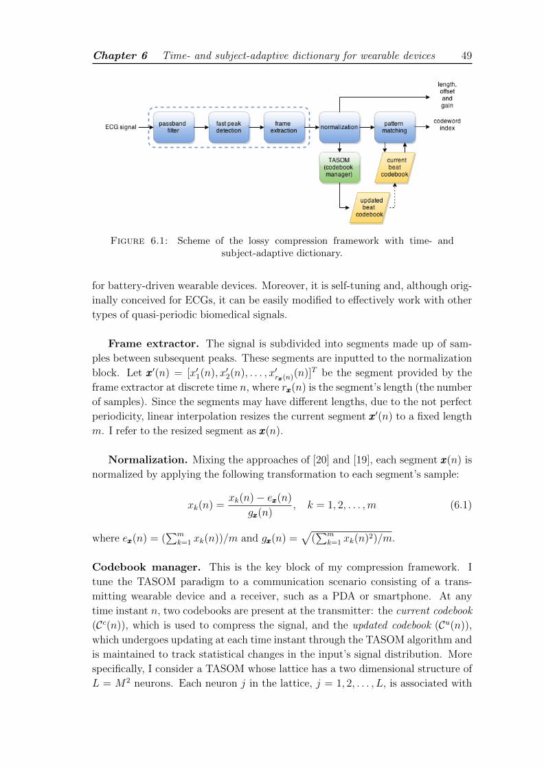
Chapter 6 Time- and subject-adaptive dictionary for wearable devices 49
Figure 6.1: Scheme of the lossy compression framework with time- andsubject-adaptive dictionary.
for battery-driven wearable devices. Moreover, it is self-tuning and, although orig-
inally conceived for ECGs, it can be easily modified to effectively work with other
types of quasi-periodic biomedical signals.
Frame extractor. The signal is subdivided into segments made up of sam-
ples between subsequent peaks. These segments are inputted to the normalization
block. Let xxx′(n) = [x′1(n), x′2(n), . . . , x′rxxx(n)(n)]T be the segment provided by the
frame extractor at discrete time n, where rxxx(n) is the segment’s length (the number
of samples). Since the segments may have different lengths, due to the not perfect
periodicity, linear interpolation resizes the current segment xxx′(n) to a fixed length
m. I refer to the resized segment as xxx(n).
Normalization. Mixing the approaches of [20] and [19], each segment xxx(n) is
normalized by applying the following transformation to each segment’s sample:
xk(n) =xk(n)− exxx(n)
gxxx(n), k = 1, 2, . . . ,m (6.1)
where exxx(n) = (∑m
k=1 xk(n))/m and gxxx(n) =√
(∑m
k=1 xk(n)2)/m.
Codebook manager. This is the key block of my compression framework. I
tune the TASOM paradigm to a communication scenario consisting of a trans-
mitting wearable device and a receiver, such as a PDA or smartphone. At any
time instant n, two codebooks are present at the transmitter: the current codebook
(Cc(n)), which is used to compress the signal, and the updated codebook (Cu(n)),
which undergoes updating at each time instant through the TASOM algorithm and
is maintained to track statistical changes in the input’s signal distribution. More
specifically, I consider a TASOM whose lattice has a two dimensional structure of
L = M2 neurons. Each neuron j in the lattice, j = 1, 2, . . . , L, is associated with

Chapter 6 Time- and subject-adaptive dictionary for wearable devices 50
a synaptic-weight vector wwwj with m components, see Equation (5.2). When the
compression scheme is activated for the first time, a sufficient number N of seg-
ments are given as input to the TASOM to perform a preliminary training phase
through Algorithm 3. Such training allows the map to learn the subject signal’s
distribution. This may be accomplished the first time the subject wears the device
and, as I will quantify in the next Chapter 7, requires less than an hour for excellent
accuracy. After this, a first subject-specific codebook is available. It can be used
for compression and can also be updated at runtime as more data is acquired.
Let assume that time is reset when the preliminary training ends and let be n = 0
at such point. Both Cc(0) = {cccc1(0), , . . . , ccccL(0)} and Cu(0) = {cccu1(0), , . . . , cccuL(0)}are defined as the codebooks whose codewords ccc∗∗(0) are equal to the synaptic-
weight vectors of the TASOM. At time n = 0, it holds: ccccj(0) = cccuj (0) = wwwj(0),
j = 1, , . . . , L. It is also assumed that the decompressor at the receiver is synchro-
nized with the compressor, i.e., it owns a copy of Cc(0). From time 0 onwards, for
any new segment xxx(n), n = 1, 2, . . . the following procedure is followed:
Algorithm 4 (Time- and subject-adaptive dictionary
for wearable devices).
1. Map xxx(n) onto the index of the best matching codeword in Cc(n), i.e., map
xxx(n) onto the index ixxx(n) such that
ixxx(n) = argminj ‖xxx(n)− ccccj(n)‖ , j = 1, . . . , L . (6.2)
Let d(n) = ‖xxx(n) − cccci(n)‖ be the Euclidean distance between the current
segment and the associated codeword, where we use index i as a shorthand
notation for ixxx(n).
2. Usexxx(n) as the new input for Algorithm 3 and obtain the new synaptic-weight
vectors wwwj(n), j = 1, . . . , L.
3. Update Cu(n) by using the weights obtained in step 2, i.e., setting
cccuj (n)← wwwj(n), j = 1, . . . , L . (6.3)
4. Let ε > 0 be a tuning parameter. If d(n)/‖xxx(n)‖ > ε, then update Cc(n) by
replacing it with Cu(n), i.e., Cc(n) ← Cu(n) and re-map xxx(n) onto the index
of the best matching codeword in the new codebook Cc(n), i.e., map xxx(n)
onto the index ixxx(n) obtained through (6.2) using the new codebook Cc(n).
5. Send to the receiver the segment’s original length rxxx(n), its offset exxx(n),
gain gxxx(n), and the codeword index ixxx(n). If the current codebook has been
Chapter 6 Time- and subject-adaptive dictionary for wearable devices 51
changed in step 4, then also send Cu(n).
Step 1 performs the VQ of segment xxx(n) by using the current codebook. Step
2 and 3 make it possible to always maintain an updated approximation of the in-
put distribution at the transmitter through the updated codebook. Step 4 checks
the validity of the approximation provided by the current codebook (the currently
used codebook, which is also known at the receiver). The tunable parameter ε
controls the signal reconstruction fidelity at the decompressor: if d(n)/‖xxx(n)‖ ≤ ε,
codeword ccccixxx(n)(n) is assumed to be a suitable representation of the current seg-
ment, otherwise Cc(n) is replaced by the updated codebook Cu(n) and the encoding
mapping is re-executed. Step 5 governs the interaction of the transmitter with the
receiver: the four values representing the encoded segment (original lenght, offset,
gain, and codeword index) are sent to the latter, together with the current code-
book, provided that the current codebook at the transmitter was no longer valid
and has been replaced by the updated codebook.
Note that the higher ε, the higher the error tolerance and the lower the number
of updates of the current codebook, which is correspondingly deemed well repre-
sentative most of the time. On the contrary, a small ε entails frequent codebook
updates: this, besides regulating the actual representation error, also determines
the maximum achievable compression efficiency. This is further discussed in the
next Chapter 7. Moreover, note that every time a best matching codeword is to
be found (Equation (6.2)), I adopt the fast codebook search algorithm 1 to avoid
useless comparisons, as discussed in Sub-Sections 3.2.2 and 3.2.3.
At the receiver, the nth segment is reconstructed by picking the codeword with
index ixxx(n) from the local codebook, performing renormalization of such codeword
with respect to offset exxx(n) and gain gxxx(n) and stretching the codeword according
to the actual segment length rxxx(n).
Chapter 7
Results
7.1 Databases and performance metrics
The MIT-BIH Arrhythmia Database, the MIT-BIH Normal Sinus Rhythm Database,
and the MIMIC II Database, all found at the Physionet website [58], are used to
test the proposed compression algorithm and compare it against other known com-
pression methods from the state-of-the-art. The MIT-BIH Arrhythmia Database
was the first generally available set of standard test material for the evaluation of
arrhythmia detectors, and it has been used for that purpose as well as for research
into cardiac dynamics and validation of compression or QRS detection algorithms
in many sites and literary works worldwide since 1980. It contains 48 half-hour
traces of ambulatory ECG signals collected from both inpatients and outpatients
and digitized at 360 samples per second with 11-bit resolution. The MIT-BIH
Normal Sinus Rhythm Database includes 18 long-term ECG recordings of subjects
found to have had no significant arrhythmias. The recordings are digitized at 128
samples per second with 12-bit resolution. I do not draw extensively from this
database and exploit it essentially for the grater length of its traces for a few as-
sessments. The MIMIC II Database claims a greater variety of physiological signals
other than ECG, among which there are PPG, ABP and RESP signals. They are
recorded at 125 samples per second with variable resolutions.
For the numerical results in this thesis, I consider two types of biomedical sig-
nals, namely the ECG and the PPG, since electrocardiography and photoplethys-
mography are the two primary technologies available in wearable devices, both
specialistic and commercial. The inspection of ECG and PPG wafeforms repre-
sents a fundamental screening tool to assess the health status of an individual.
Moreover, a number of vital parameters (e.g., heart rate, respiration rate, blood
pressure) can be extracted from them to provide a more complete clinical picture.
I take into account the following performance metrics:
• Learning and adaptation time. I estimate the learning time of the pro-
posed compression scheme, which corresponds to the time needed to build up
52
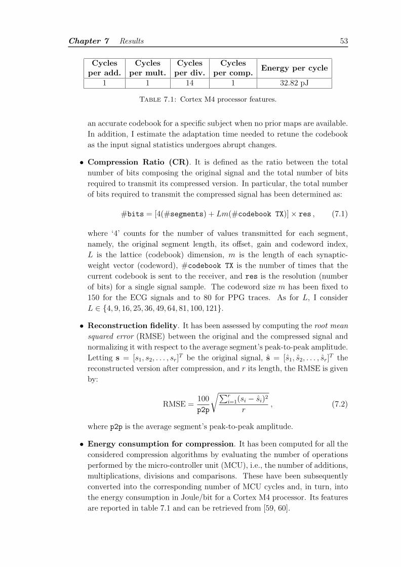
Chapter 7 Results 53
Cyclesper add.
Cyclesper mult.
Cyclesper div.
Cyclesper comp.
Energy per cycle
1 1 14 1 32.82 pJ
Table 7.1: Cortex M4 processor features.
an accurate codebook for a specific subject when no prior maps are available.
In addition, I estimate the adaptation time needed to retune the codebook
as the input signal statistics undergoes abrupt changes.
• Compression Ratio (CR). It is defined as the ratio between the total
number of bits composing the original signal and the total number of bits
required to transmit its compressed version. In particular, the total number
of bits required to transmit the compressed signal has been determined as:
#bits = [4(#segments) + Lm(#codebook TX)]× res , (7.1)
where ‘4’ counts for the number of values transmitted for each segment,
namely, the original segment length, its offset, gain and codeword index,
L is the lattice (codebook) dimension, m is the length of each synaptic-
weight vector (codeword), #codebook TX is the number of times that the
current codebook is sent to the receiver, and res is the resolution (number
of bits) for a single signal sample. The codeword size m has been fixed to
150 for the ECG signals and to 80 for PPG traces. As for L, I consider
L ∈ {4, 9, 16, 25, 36, 49, 64, 81, 100, 121}.
• Reconstruction fidelity. It has been assessed by computing the root mean
squared error (RMSE) between the original and the compressed signal and
normalizing it with respect to the average segment’s peak-to-peak amplitude.
Letting s = [s1, s2, . . . , sr]T be the original signal, s = [s1, s2, . . . , sr]
T the
reconstructed version after compression, and r its length, the RMSE is given
by:
RMSE =100
p2p
√∑ri=1(si − si)2
r, (7.2)
where p2p is the average segment’s peak-to-peak amplitude.
• Energy consumption for compression. It has been computed for all the
considered compression algorithms by evaluating the number of operations
performed by the micro-controller unit (MCU), i.e., the number of additions,
multiplications, divisions and comparisons. These have been subsequently
converted into the corresponding number of MCU cycles and, in turn, into
the energy consumption in Joule/bit for a Cortex M4 processor. Its features
are reported in table 7.1 and can be retrieved from [59, 60].
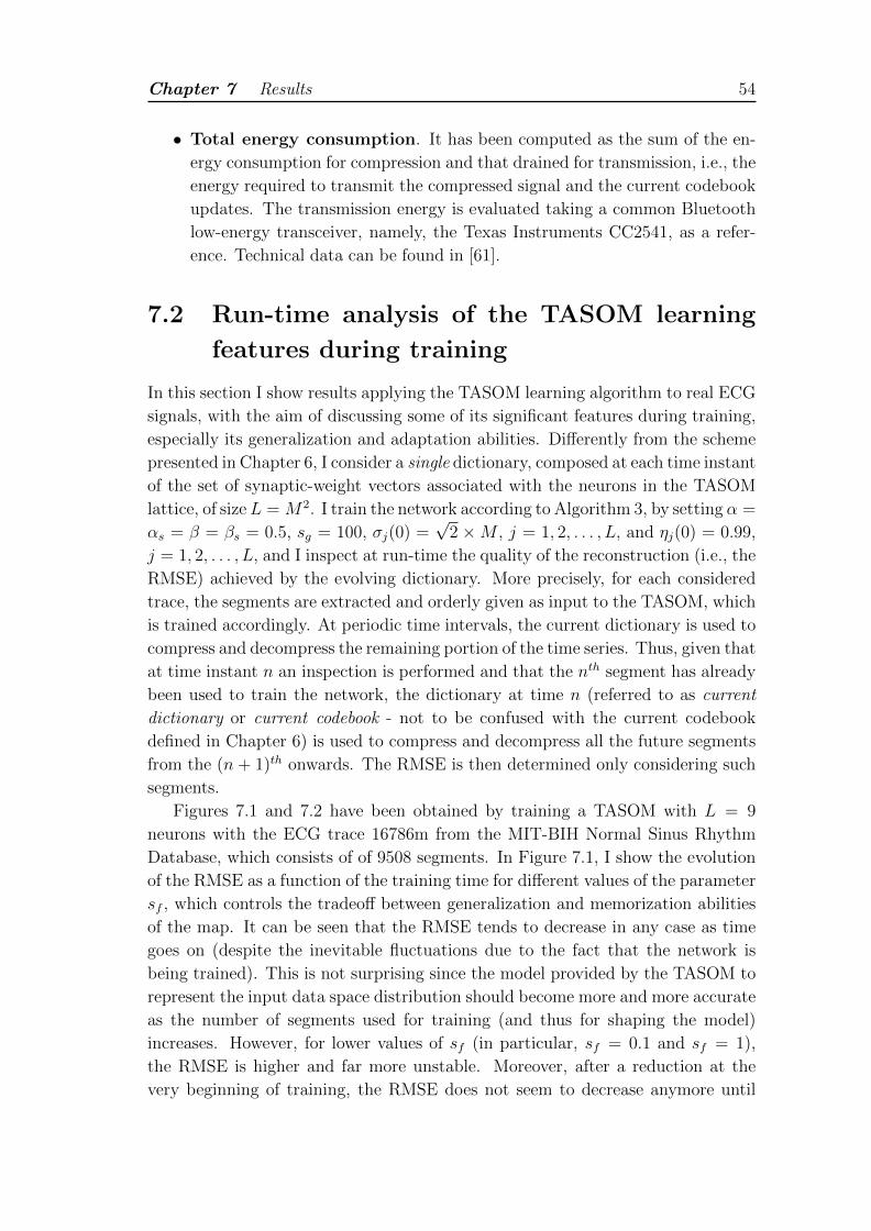
Chapter 7 Results 54
• Total energy consumption. It has been computed as the sum of the en-
ergy consumption for compression and that drained for transmission, i.e., the
energy required to transmit the compressed signal and the current codebook
updates. The transmission energy is evaluated taking a common Bluetooth
low-energy transceiver, namely, the Texas Instruments CC2541, as a refer-
ence. Technical data can be found in [61].
7.2 Run-time analysis of the TASOM learning
features during training
In this section I show results applying the TASOM learning algorithm to real ECG
signals, with the aim of discussing some of its significant features during training,
especially its generalization and adaptation abilities. Differently from the scheme
presented in Chapter 6, I consider a single dictionary, composed at each time instant
of the set of synaptic-weight vectors associated with the neurons in the TASOM
lattice, of sizeL = M2. I train the network according to Algorithm 3, by setting α =
αs = β = βs = 0.5, sg = 100, σj(0) =√
2 ×M , j = 1, 2, . . . , L, and ηj(0) = 0.99,
j = 1, 2, . . . , L, and I inspect at run-time the quality of the reconstruction (i.e., the
RMSE) achieved by the evolving dictionary. More precisely, for each considered
trace, the segments are extracted and orderly given as input to the TASOM, which
is trained accordingly. At periodic time intervals, the current dictionary is used to
compress and decompress the remaining portion of the time series. Thus, given that
at time instant n an inspection is performed and that the nth segment has already
been used to train the network, the dictionary at time n (referred to as current
dictionary or current codebook - not to be confused with the current codebook
defined in Chapter 6) is used to compress and decompress all the future segments
from the (n + 1)th onwards. The RMSE is then determined only considering such
segments.
Figures 7.1 and 7.2 have been obtained by training a TASOM with L = 9
neurons with the ECG trace 16786m from the MIT-BIH Normal Sinus Rhythm
Database, which consists of of 9508 segments. In Figure 7.1, I show the evolution
of the RMSE as a function of the training time for different values of the parameter
sf , which controls the tradeoff between generalization and memorization abilities
of the map. It can be seen that the RMSE tends to decrease in any case as time
goes on (despite the inevitable fluctuations due to the fact that the network is
being trained). This is not surprising since the model provided by the TASOM to
represent the input data space distribution should become more and more accurate
as the number of segments used for training (and thus for shaping the model)
increases. However, for lower values of sf (in particular, sf = 0.1 and sf = 1),
the RMSE is higher and far more unstable. Moreover, after a reduction at the
very beginning of training, the RMSE does not seem to decrease anymore until
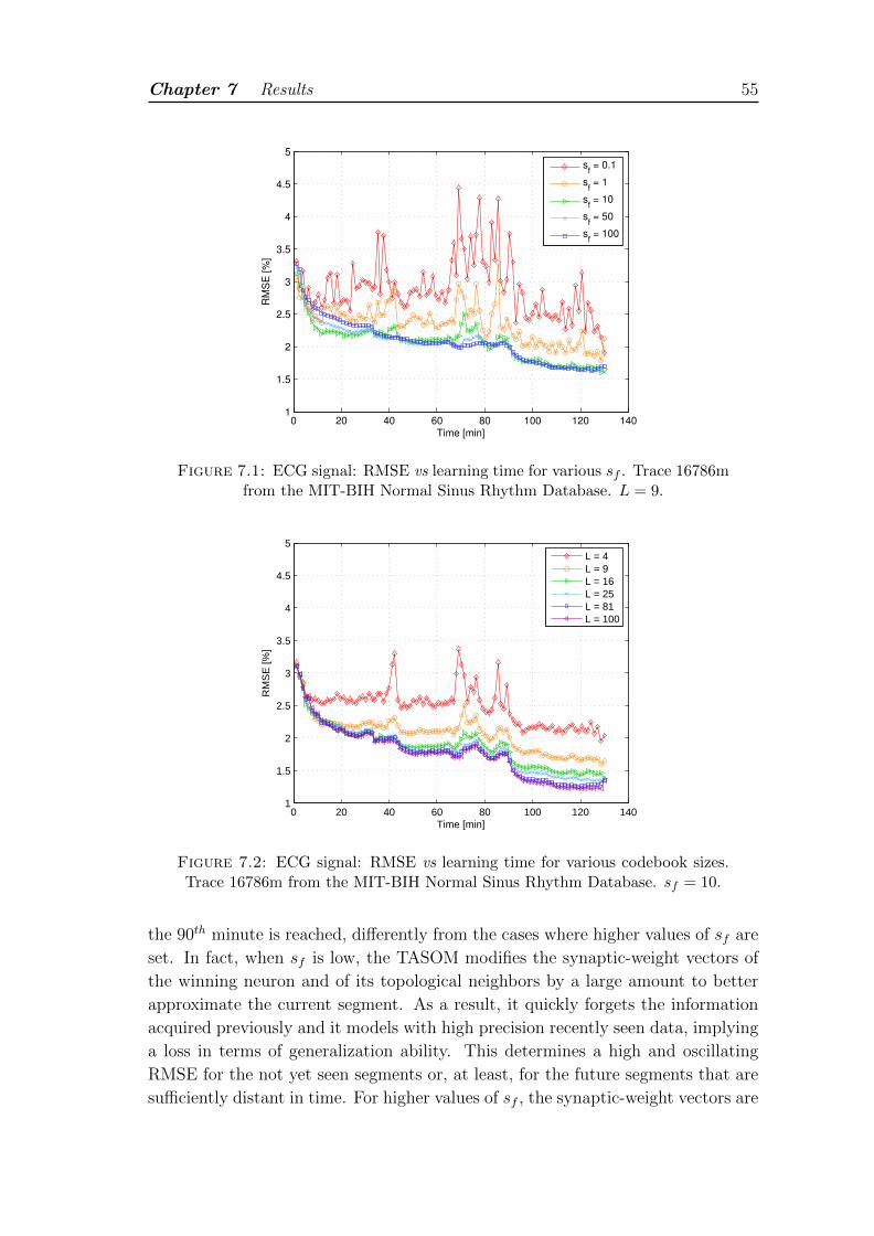
Chapter 7 Results 55
0 20 40 60 80 100 120 1401
1.5
2
2.5
3
3.5
4
4.5
5
Time [min]
RM
SE
[%
]
sf = 0.1
sf = 1
sf = 10
sf = 50
sf = 100
Figure 7.1: ECG signal: RMSE vs learning time for various sf . Trace 16786mfrom the MIT-BIH Normal Sinus Rhythm Database. L = 9.
0 20 40 60 80 100 120 1401
1.5
2
2.5
3
3.5
4
4.5
5
Time [min]
RM
SE
[%]
L = 4L = 9L = 16L = 25L = 81L = 100
Figure 7.2: ECG signal: RMSE vs learning time for various codebook sizes.Trace 16786m from the MIT-BIH Normal Sinus Rhythm Database. sf = 10.
the 90th minute is reached, differently from the cases where higher values of sf are
set. In fact, when sf is low, the TASOM modifies the synaptic-weight vectors of
the winning neuron and of its topological neighbors by a large amount to better
approximate the current segment. As a result, it quickly forgets the information
acquired previously and it models with high precision recently seen data, implying
a loss in terms of generalization ability. This determines a high and oscillating
RMSE for the not yet seen segments or, at least, for the future segments that are
sufficiently distant in time. For higher values of sf , the synaptic-weight vectors are
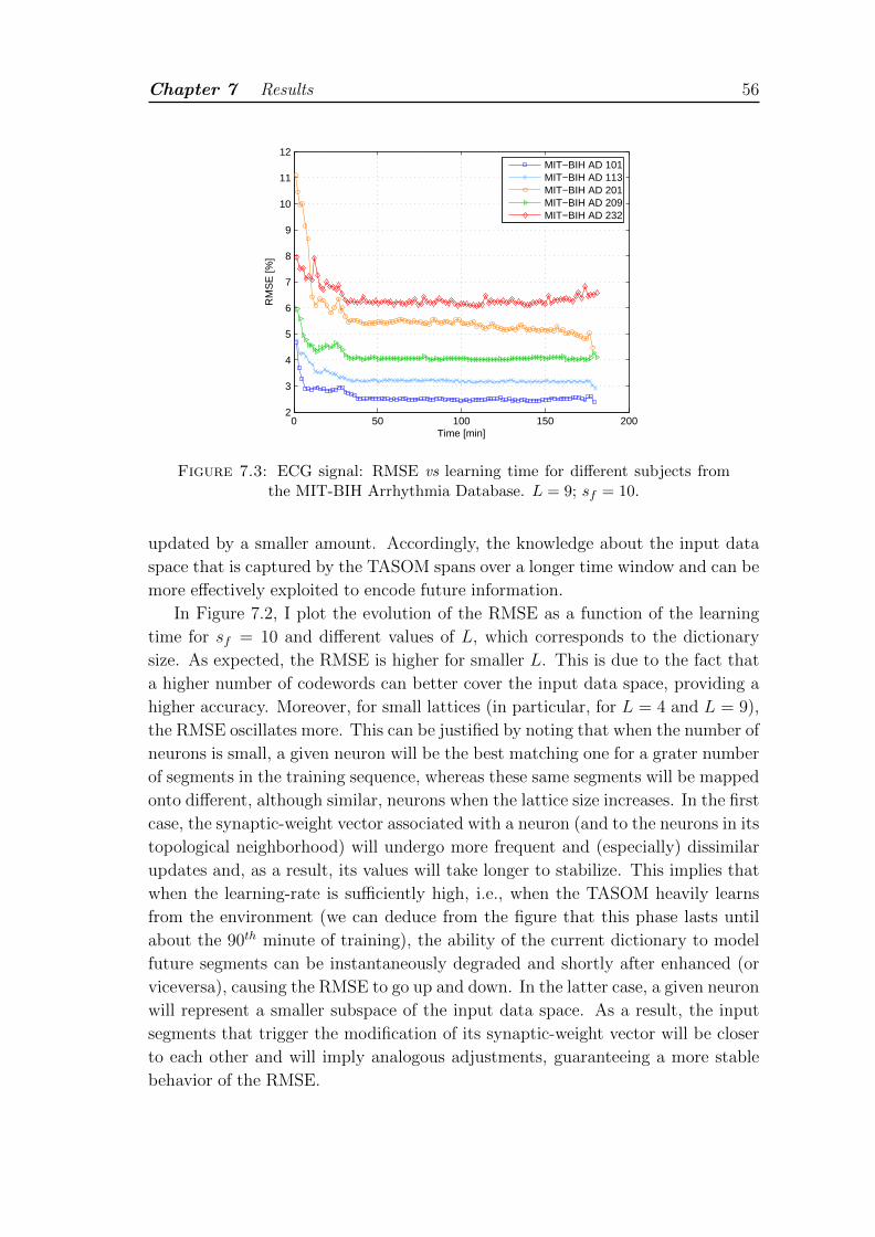
Chapter 7 Results 56
0 50 100 150 2002
3
4
5
6
7
8
9
10
11
12
Time [min]
RM
SE
[%]
MIT−BIH AD 101MIT−BIH AD 113MIT−BIH AD 201MIT−BIH AD 209MIT−BIH AD 232
Figure 7.3: ECG signal: RMSE vs learning time for different subjects fromthe MIT-BIH Arrhythmia Database. L = 9; sf = 10.
updated by a smaller amount. Accordingly, the knowledge about the input data
space that is captured by the TASOM spans over a longer time window and can be
more effectively exploited to encode future information.
In Figure 7.2, I plot the evolution of the RMSE as a function of the learning
time for sf = 10 and different values of L, which corresponds to the dictionary
size. As expected, the RMSE is higher for smaller L. This is due to the fact that
a higher number of codewords can better cover the input data space, providing a
higher accuracy. Moreover, for small lattices (in particular, for L = 4 and L = 9),
the RMSE oscillates more. This can be justified by noting that when the number of
neurons is small, a given neuron will be the best matching one for a grater number
of segments in the training sequence, whereas these same segments will be mapped
onto different, although similar, neurons when the lattice size increases. In the first
case, the synaptic-weight vector associated with a neuron (and to the neurons in its
topological neighborhood) will undergo more frequent and (especially) dissimilar
updates and, as a result, its values will take longer to stabilize. This implies that
when the learning-rate is sufficiently high, i.e., when the TASOM heavily learns
from the environment (we can deduce from the figure that this phase lasts until
about the 90th minute of training), the ability of the current dictionary to model
future segments can be instantaneously degraded and shortly after enhanced (or
viceversa), causing the RMSE to go up and down. In the latter case, a given neuron
will represent a smaller subspace of the input data space. As a result, the input
segments that trigger the modification of its synaptic-weight vector will be closer
to each other and will imply analogous adjustments, guaranteeing a more stable
behavior of the RMSE.
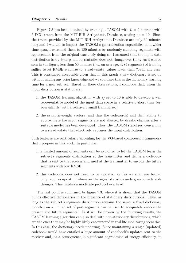
Chapter 7 Results 57
Figure 7.3 has been obtained by training a TASOM with L = 9 neurons with
5 ECG traces from the MIT-BIH Arrhythmia Database, setting sf = 10. Since
the traces provided by the MIT-BIH Arrhythmia Database are only 30 minutes
long and I wanted to inspect the TASOM’s generalization capabilities on a wider
time span, I extended them to 180 minutes by randomly sampling segments with
replacement from the original trace. By doing so, I assumed that the input data
distribution is stationary, i.e., its statistics does not change over time. As it can be
seen in the figure, less than 50 minutes (i.e., on average, 4285 segments) of training
suffice to let RMSE stabilize to ‘steady-state’ values lower than 7% in any case.
This is considered acceptable given that in this graph a new dictionary is set up
without having any prior knowledge and we could see this as the dictionary learning
time for a new subject. Based on these observations, I conclude that, when the
input distribution is stationary:
1. the TASOM learning algorithm with sf set to 10 is able to develop a well
representative model of the input data space in a relatively short time (or,
equivalently, with a relatively small training set);
2. the synaptic-weight vectors (and thus the codewords) and their ability to
approximate the input segments are not affected by drastic changes after a
suitable model has been developed. Thus, the TASOM stabilizes, converging
to a steady-state that effectively captures the input distribution.
Such features are particularly appealing for the VQ-based compression framework
that I propose in this work. In particular:
1. a limited amount of segments can be exploited to let the TASOM learn the
subject’s segments distribution at the transmitter and define a codebook
that is sent to the receiver and used at the transmitter to encode the future
segments with low RMSE;
2. this codebook does not need to be updated, or (as we shall see below)
only requires updating whenever the signal statistics undergoes considerable
changes. This implies a moderate protocol overhead.
The last point is confirmed by figure 7.3, where it is shown that the TASOM
builds effective dictionaries in the presence of stationary distributions. Thus, as
long as the subject’s segments distribution remains the same, a fixed dictionary
modeled on a limited set of past segments can be used to adequately encode the
present and future segments. As it will be proven by the following results, the
TASOM learning algorithm can also deal with non-stationary distributions, which
are the ones that may be highly likely encountered in real life monitoring scenarios.
In this case, the dictionary needs updating. Since maintaining a single (updated)
codebook would have entailed a huge amount of codebook’s updates sent to the
receiver and, as a consequence, a significant degradation of energy efficiency, in
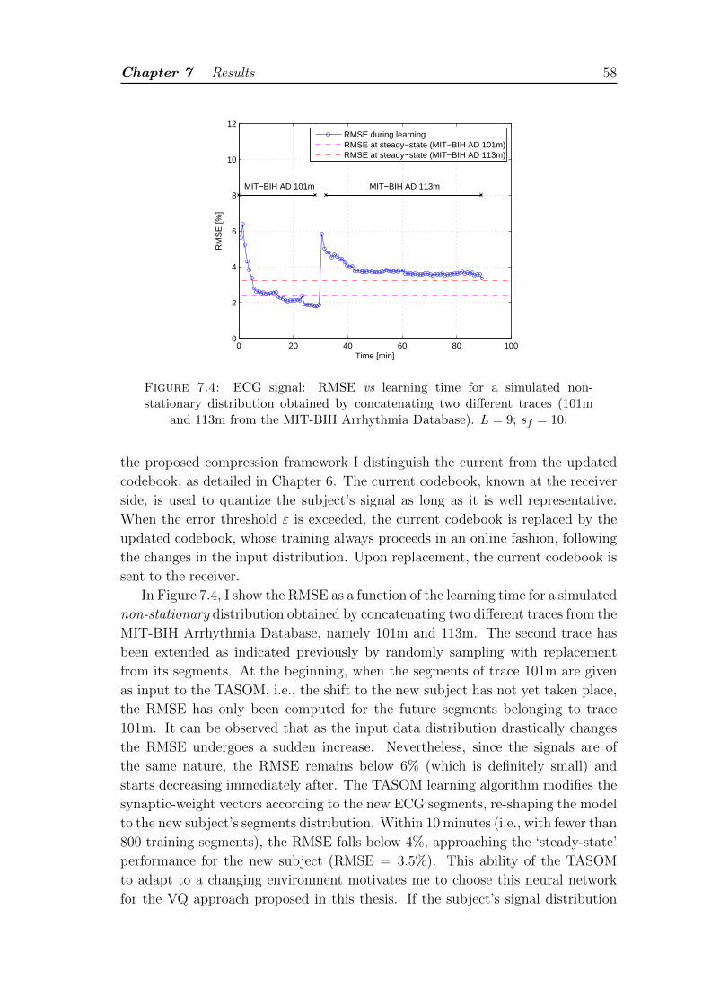
Chapter 7 Results 58
0 20 40 60 80 1000
2
4
6
8
10
12
Time [min]
RM
SE
[%]
MIT−BIH AD 101m MIT−BIH AD 113m
RMSE during learningRMSE at steady−state (MIT−BIH AD 101m)RMSE at steady−state (MIT−BIH AD 113m)
Figure 7.4: ECG signal: RMSE vs learning time for a simulated non-stationary distribution obtained by concatenating two different traces (101m
and 113m from the MIT-BIH Arrhythmia Database). L = 9; sf = 10.
the proposed compression framework I distinguish the current from the updated
codebook, as detailed in Chapter 6. The current codebook, known at the receiver
side, is used to quantize the subject’s signal as long as it is well representative.
When the error threshold ε is exceeded, the current codebook is replaced by the
updated codebook, whose training always proceeds in an online fashion, following
the changes in the input distribution. Upon replacement, the current codebook is
sent to the receiver.
In Figure 7.4, I show the RMSE as a function of the learning time for a simulated
non-stationary distribution obtained by concatenating two different traces from the
MIT-BIH Arrhythmia Database, namely 101m and 113m. The second trace has
been extended as indicated previously by randomly sampling with replacement
from its segments. At the beginning, when the segments of trace 101m are given
as input to the TASOM, i.e., the shift to the new subject has not yet taken place,
the RMSE has only been computed for the future segments belonging to trace
101m. It can be observed that as the input data distribution drastically changes
the RMSE undergoes a sudden increase. Nevertheless, since the signals are of
the same nature, the RMSE remains below 6% (which is definitely small) and
starts decreasing immediately after. The TASOM learning algorithm modifies the
synaptic-weight vectors according to the new ECG segments, re-shaping the model
to the new subject’s segments distribution. Within 10 minutes (i.e., with fewer than
800 training segments), the RMSE falls below 4%, approaching the ‘steady-state’
performance for the new subject (RMSE = 3.5%). This ability of the TASOM
to adapt to a changing environment motivates me to choose this neural network
for the VQ approach proposed in this thesis. If the subject’s signal distribution
Chapter 7 Results 59
changes, due to the subject’s activities or due to physiological causes, it is extremely
important to dynamically adjust the set of codewords to the evolving statistics, and
the TASOM satisfies such requirement.
7.3 Performance analysis of the time- and
subject-adaptive compression method -
the choice of sf and L
In this section, I present a set of results obtained by running the proposed compres-
sion method on the trace 113m from the MIT-BIH Arrhythmia Database. This set
aims at justifying the choices of two main parameters, namely, sf (generalization
parameter) and L (lattice/dictionaries size). The fine tuning of these parameters is
particularly important for the results presented in Section 7.4, where the proposed
algorithm is compared with other common compression approaches. I consider
a single trace for simplicity. Analogous considerations could have been done by
taking into account a grater number of traces.
The TASOM preliminary training phase (see Chapter 6) was executed by giving
as input to the TASOM N = L × 500 + 1000 segments, picked at random (with
replacement) from the first three minutes of the 113m record. In all the experiments
I set α = αs = β = βs = 0.5, sg = 100, σj(0) =√
2 ×M , j = 1, 2, . . . , L, and
ηj(0) = 0.99, j = 1, 2, . . . , L. The evaluations are carried out by considering the
effects of compression on the last 27 minutes of the ECG record, i.e., the section
that does not contribute to the preliminary training phase.
Unless otherwise stated, the curves in the graphs have been derived by letting
the parameter ε vary. Recall that ε controls the signal reconstruction fidelity at the
decompressor: if the distance between the current segment and the corresponding
codeword in the current codebook exceeds ε times the norm of the segment (i.e.,
if d(n)/‖x(n)‖ > ε), then the reconstruction fidelity is considered unsatisfactory,
the current codebook undergoes updating and the new matching codeword is de-
termined. As ε increases, the number of updates decreases and the CR increases
accordingly.
In Figure 7.5, I plot the RMSE against the compression ratio for a TASOM
lattice made by L = 9 neurons. Each curve is associated with a different value
of the parameter sf . It can be noticed that when the CR is low (and the number
of updates is correspondingly high), smaller values of sf perform better in terms
of RMSE. Indeed, when sf is small, the TASOM privileges the most recent input
segments, heavily modifying the synaptic-weight vectors (winning and neighbor-
hood) to pull them towards such segments. This implies that, for a given number
of current codebook’s updates, the relative error upon reconstruction is lower than
that achieved by the TASOM when sf is higher, because the evolving codewords
are less closer to the individual ECG segments in the latter case. As the parameter
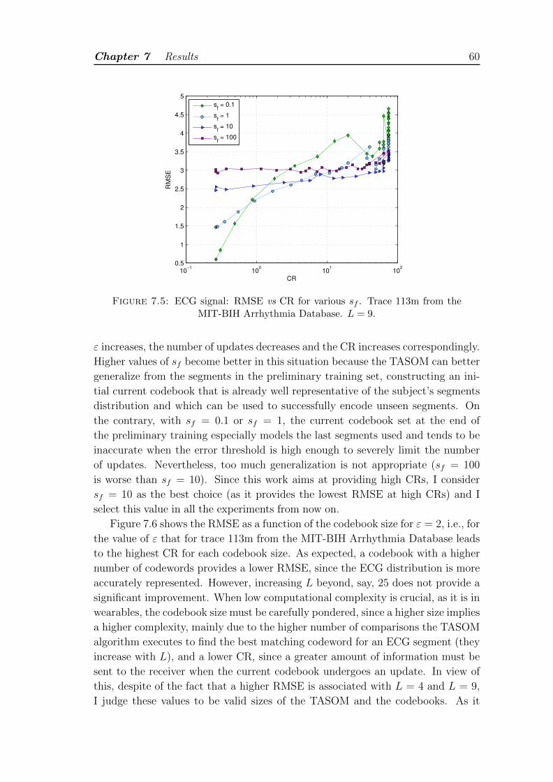
Chapter 7 Results 60
10−1
100
101
102
0.5
1
1.5
2
2.5
3
3.5
4
4.5
5
CR
RM
SE
sf = 0.1
sf = 1
sf = 10
sf = 100
Figure 7.5: ECG signal: RMSE vs CR for various sf . Trace 113m from theMIT-BIH Arrhythmia Database. L = 9.
ε increases, the number of updates decreases and the CR increases correspondingly.
Higher values of sf become better in this situation because the TASOM can better
generalize from the segments in the preliminary training set, constructing an ini-
tial current codebook that is already well representative of the subject’s segments
distribution and which can be used to successfully encode unseen segments. On
the contrary, with sf = 0.1 or sf = 1, the current codebook set at the end of
the preliminary training especially models the last segments used and tends to be
inaccurate when the error threshold is high enough to severely limit the number
of updates. Nevertheless, too much generalization is not appropriate (sf = 100
is worse than sf = 10). Since this work aims at providing high CRs, I consider
sf = 10 as the best choice (as it provides the lowest RMSE at high CRs) and I
select this value in all the experiments from now on.
Figure 7.6 shows the RMSE as a function of the codebook size for ε = 2, i.e., for
the value of ε that for trace 113m from the MIT-BIH Arrhythmia Database leads
to the highest CR for each codebook size. As expected, a codebook with a higher
number of codewords provides a lower RMSE, since the ECG distribution is more
accurately represented. However, increasing L beyond, say, 25 does not provide a
significant improvement. When low computational complexity is crucial, as it is in
wearables, the codebook size must be carefully pondered, since a higher size implies
a higher complexity, mainly due to the higher number of comparisons the TASOM
algorithm executes to find the best matching codeword for an ECG segment (they
increase with L), and a lower CR, since a greater amount of information must be
sent to the receiver when the current codebook undergoes an update. In view of
this, despite of the fact that a higher RMSE is associated with L = 4 and L = 9,
I judge these values to be valid sizes of the TASOM and the codebooks. As it
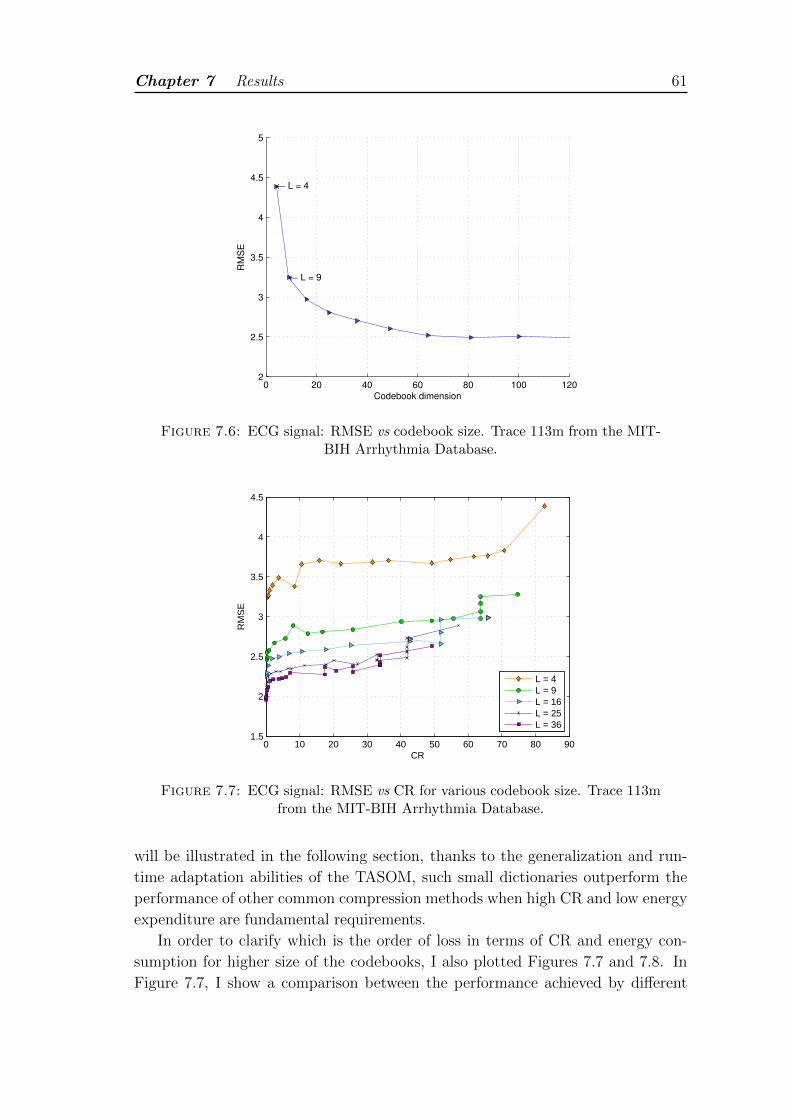
Chapter 7 Results 61
0 20 40 60 80 100 1202
2.5
3
3.5
4
4.5
5
Codebook dimension
RM
SE
← L = 4
← L = 9
Figure 7.6: ECG signal: RMSE vs codebook size. Trace 113m from the MIT-BIH Arrhythmia Database.
0 10 20 30 40 50 60 70 80 901.5
2
2.5
3
3.5
4
4.5
CR
RM
SE
L = 4L = 9L = 16L = 25L = 36
Figure 7.7: ECG signal: RMSE vs CR for various codebook size. Trace 113mfrom the MIT-BIH Arrhythmia Database.
will be illustrated in the following section, thanks to the generalization and run-
time adaptation abilities of the TASOM, such small dictionaries outperform the
performance of other common compression methods when high CR and low energy
expenditure are fundamental requirements.
In order to clarify which is the order of loss in terms of CR and energy con-
sumption for higher size of the codebooks, I also plotted Figures 7.7 and 7.8. In
Figure 7.7, I show a comparison between the performance achieved by different
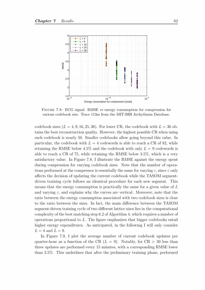
Chapter 7 Results 62
10−11
10−10
10−9
1.5
2
2.5
3
3.5
4
4.5
5
Energy consumption for compression [Joule]
RM
SE
L = 4L = 9L = 16L = 25L = 36
Figure 7.8: ECG signal: RMSE vs energy consumption for compression forvarious codebook size. Trace 113m from the MIT-BIH Arrhythmia Database.
codebook sizes (L = 4, 9, 16, 25, 36). For lower CR, the codebook with L = 36 ob-
tains the best reconstruction quality. However, the highest possible CR when using
such codebook is nearly 50. Smaller codebooks allow going beyond this value. In
particular, the codebook with L = 4 codewords is able to reach a CR of 82, while
retaining the RMSE below 4.5% and the codebook with only L = 9 codewords is
able to reach a CR of 75, while retaining the RMSE below 3.5%, which is a very
satisfactory value. In Figure 7.8, I illustrate the RMSE against the energy spent
during compression for varying codebook sizes. Note that the number of opera-
tions performed at the compressor is essentially the same for varying ε, since ε only
affects the decision of updating the current codebook while the TASOM segment-
driven training cycle follows an identical procedure for each new segment. This
means that the energy consumption is practically the same for a given value of L
and varying ε, and explains why the curves are vertical. Moreover, note that the
ratio between the energy consumption associated with two codebook sizes is close
to the ratio between the sizes. In fact, the main difference between the TASOM
segment-driven training cycle of two different lattice sizes lies in the computational
complexity of the best matching step 6.2 of Algorithm 4, which requires a number of
operations proportional to L. The figure emphasizes that bigger codebooks entail
higher energy expenditures. As anticipated, in the following I will only consider
L = 4 and L = 9.
In Figure 7.9, I plot the average number of current codebook updates per
quarter-hour as a function of the CR (L = 9). Notably, for CR > 30 less than
three updates are performed every 15 minutes, with a corresponding RMSE lower
than 3.5%. This underlines that after the preliminary training phase, performed
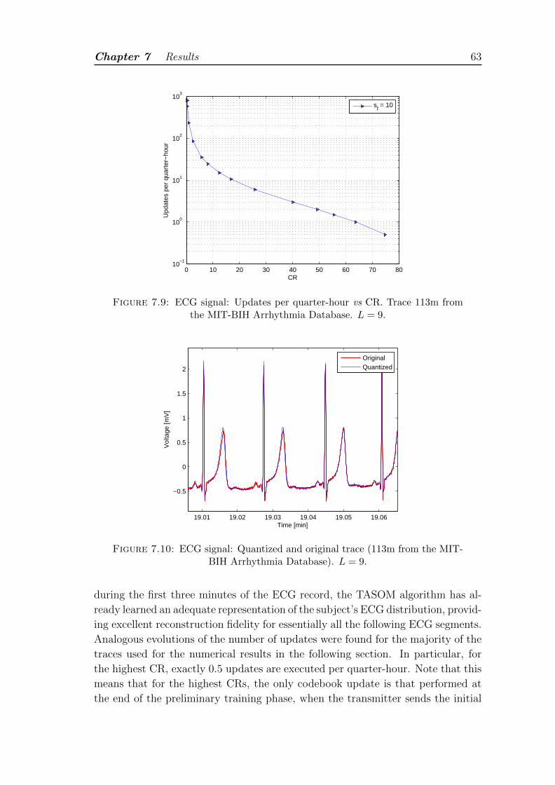
Chapter 7 Results 63
0 10 20 30 40 50 60 70 8010
−1
100
101
102
103
CR
Upd
ates
per
qua
rter
−ho
ur
s
f = 10
Figure 7.9: ECG signal: Updates per quarter-hour vs CR. Trace 113m fromthe MIT-BIH Arrhythmia Database. L = 9.
19.01 19.02 19.03 19.04 19.05 19.06
−0.5
0
0.5
1
1.5
2
Time [min]
Vol
tage
[mV
]
OriginalQuantized
Figure 7.10: ECG signal: Quantized and original trace (113m from the MIT-BIH Arrhythmia Database). L = 9.
during the first three minutes of the ECG record, the TASOM algorithm has al-
ready learned an adequate representation of the subject’s ECG distribution, provid-
ing excellent reconstruction fidelity for essentially all the following ECG segments.
Analogous evolutions of the number of updates were found for the majority of the
traces used for the numerical results in the following section. In particular, for
the highest CR, exactly 0.5 updates are executed per quarter-hour. Note that this
means that for the highest CRs, the only codebook update is that performed at
the end of the preliminary training phase, when the transmitter sends the initial

Chapter 7 Results 64
codebook to the receiver. Since the reconstruction error at high CRs is maintained
low (see the following section), this proves, once again, that the TASOM algorithm
efficiently learns from the environment, whatever distribution is presented to it.
In Figure 7.10, I provide a comparison between the original and the compressed
ECG signal to provide a visual insight into the quality of reconstruction. For this
plot I set L = 9 and ε = 2, obtaining and RMSE equal to 3.25%. The compressed
signal almost perfectly resembles the uncompressed one. Moreover, the TASOM-
based technique provides a noise-filtering function. In fact, while the original signal
presents some superimposed random noise due to artifacts, the compressed version
has a smoother face.
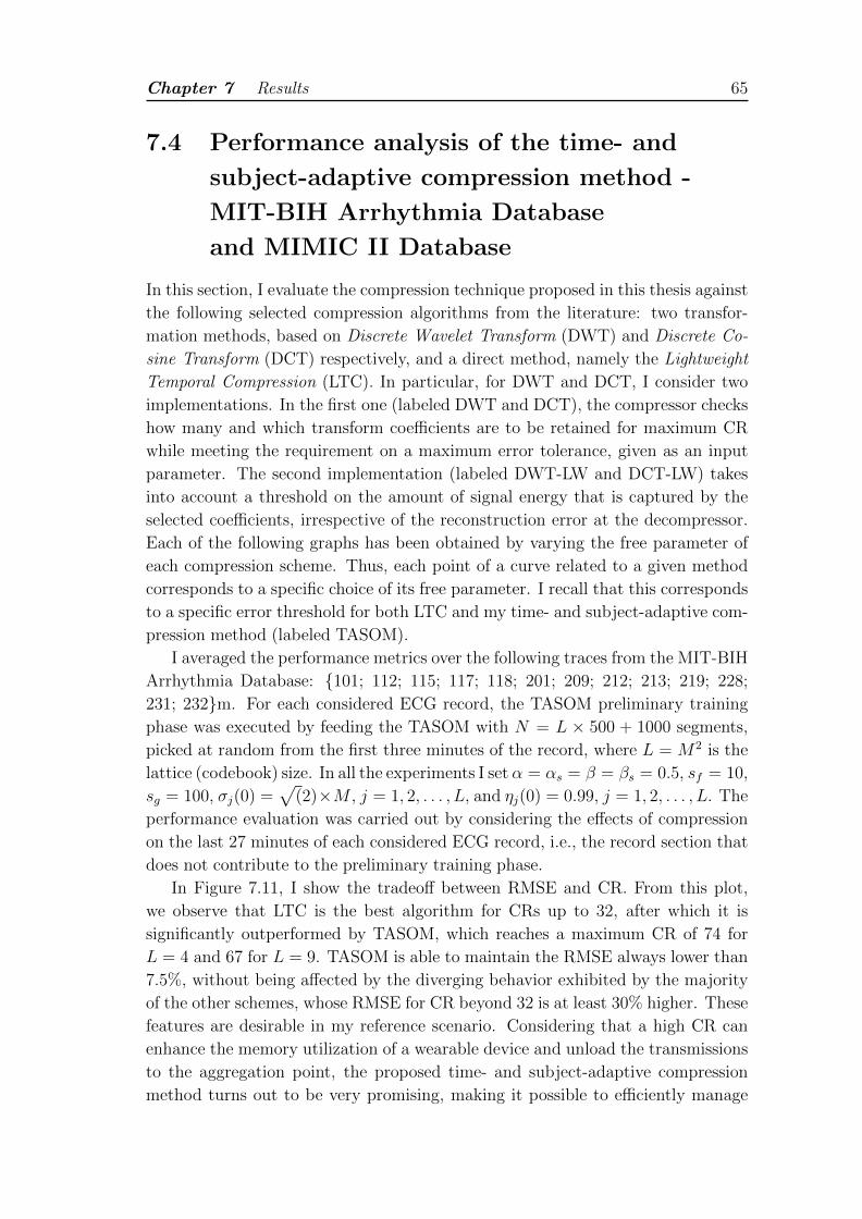
Chapter 7 Results 65
7.4 Performance analysis of the time- and
subject-adaptive compression method -
MIT-BIH Arrhythmia Database
and MIMIC II Database
In this section, I evaluate the compression technique proposed in this thesis against
the following selected compression algorithms from the literature: two transfor-
mation methods, based on Discrete Wavelet Transform (DWT) and Discrete Co-
sine Transform (DCT) respectively, and a direct method, namely the Lightweight
Temporal Compression (LTC). In particular, for DWT and DCT, I consider two
implementations. In the first one (labeled DWT and DCT), the compressor checks
how many and which transform coefficients are to be retained for maximum CR
while meeting the requirement on a maximum error tolerance, given as an input
parameter. The second implementation (labeled DWT-LW and DCT-LW) takes
into account a threshold on the amount of signal energy that is captured by the
selected coefficients, irrespective of the reconstruction error at the decompressor.
Each of the following graphs has been obtained by varying the free parameter of
each compression scheme. Thus, each point of a curve related to a given method
corresponds to a specific choice of its free parameter. I recall that this corresponds
to a specific error threshold for both LTC and my time- and subject-adaptive com-
pression method (labeled TASOM).
I averaged the performance metrics over the following traces from the MIT-BIH
Arrhythmia Database: {101; 112; 115; 117; 118; 201; 209; 212; 213; 219; 228;
231; 232}m. For each considered ECG record, the TASOM preliminary training
phase was executed by feeding the TASOM with N = L × 500 + 1000 segments,
picked at random from the first three minutes of the record, where L = M2 is the
lattice (codebook) size. In all the experiments I set α = αs = β = βs = 0.5, sf = 10,
sg = 100, σj(0) =√
(2)×M , j = 1, 2, . . . , L, and ηj(0) = 0.99, j = 1, 2, . . . , L. The
performance evaluation was carried out by considering the effects of compression
on the last 27 minutes of each considered ECG record, i.e., the record section that
does not contribute to the preliminary training phase.
In Figure 7.11, I show the tradeoff between RMSE and CR. From this plot,
we observe that LTC is the best algorithm for CRs up to 32, after which it is
significantly outperformed by TASOM, which reaches a maximum CR of 74 for
L = 4 and 67 for L = 9. TASOM is able to maintain the RMSE always lower than
7.5%, without being affected by the diverging behavior exhibited by the majority
of the other schemes, whose RMSE for CR beyond 32 is at least 30% higher. These
features are desirable in my reference scenario. Considering that a high CR can
enhance the memory utilization of a wearable device and unload the transmissions
to the aggregation point, the proposed time- and subject-adaptive compression
method turns out to be very promising, making it possible to efficiently manage
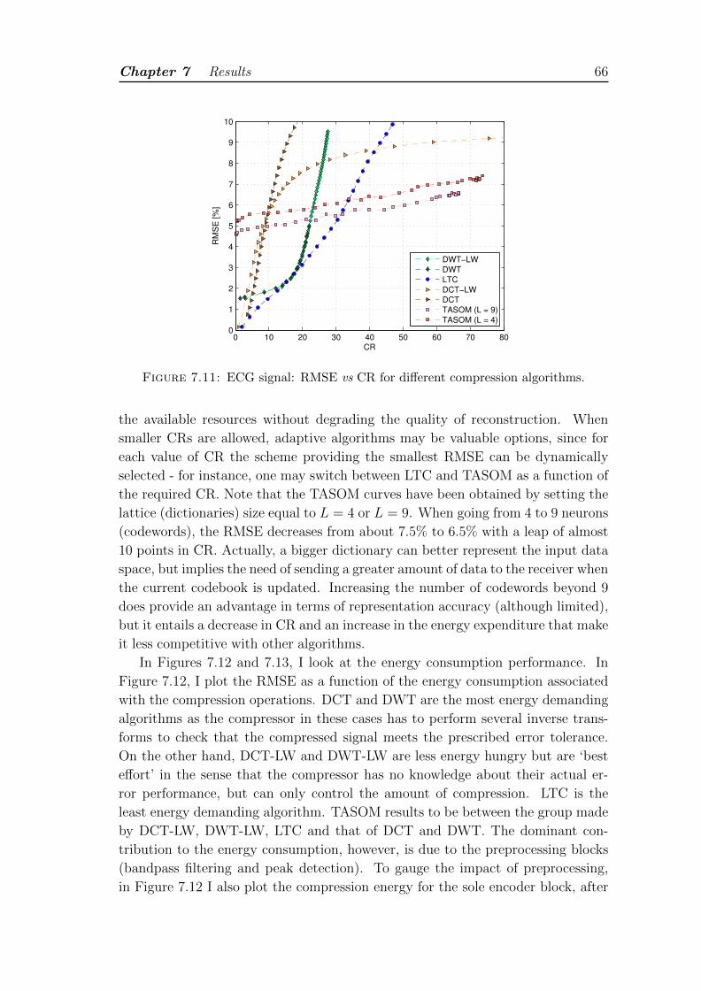
Chapter 7 Results 66
0 10 20 30 40 50 60 70 800
1
2
3
4
5
6
7
8
9
10
CR
RM
SE
[%
]
DWT−LW
DWT
LTC
DCT−LW
DCT
TASOM (L = 9)
TASOM (L = 4)
Figure 7.11: ECG signal: RMSE vs CR for different compression algorithms.
the available resources without degrading the quality of reconstruction. When
smaller CRs are allowed, adaptive algorithms may be valuable options, since for
each value of CR the scheme providing the smallest RMSE can be dynamically
selected - for instance, one may switch between LTC and TASOM as a function of
the required CR. Note that the TASOM curves have been obtained by setting the
lattice (dictionaries) size equal to L = 4 or L = 9. When going from 4 to 9 neurons
(codewords), the RMSE decreases from about 7.5% to 6.5% with a leap of almost
10 points in CR. Actually, a bigger dictionary can better represent the input data
space, but implies the need of sending a greater amount of data to the receiver when
the current codebook is updated. Increasing the number of codewords beyond 9
does provide an advantage in terms of representation accuracy (although limited),
but it entails a decrease in CR and an increase in the energy expenditure that make
it less competitive with other algorithms.
In Figures 7.12 and 7.13, I look at the energy consumption performance. In
Figure 7.12, I plot the RMSE as a function of the energy consumption associated
with the compression operations. DCT and DWT are the most energy demanding
algorithms as the compressor in these cases has to perform several inverse trans-
forms to check that the compressed signal meets the prescribed error tolerance.
On the other hand, DCT-LW and DWT-LW are less energy hungry but are ‘best
effort’ in the sense that the compressor has no knowledge about their actual er-
ror performance, but can only control the amount of compression. LTC is the
least energy demanding algorithm. TASOM results to be between the group made
by DCT-LW, DWT-LW, LTC and that of DCT and DWT. The dominant con-
tribution to the energy consumption, however, is due to the preprocessing blocks
(bandpass filtering and peak detection). To gauge the impact of preprocessing,
in Figure 7.12 I also plot the compression energy for the sole encoder block, after
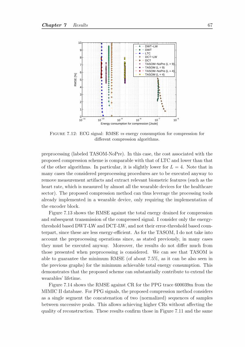
Chapter 7 Results 67
10−11
10−10
10−9
10−8
10−7
10−6
0
1
2
3
4
5
6
7
8
9
10
Energy consumption for compression [Joule]
RM
SE
[%]
DWT−LWDWTLTCDCT−LWDCTTASOM−NoPre (L = 9)TASOM (L = 9)TASOM−NoPre (L = 4)TASOM (L = 4)
Figure 7.12: ECG signal: RMSE vs energy consumption for compression fordifferent compression algorithms.
preprocessing (labeled TASOM-NoPre). In this case, the cost associated with the
proposed compression scheme is comparable with that of LTC and lower than that
of the other algorithms. In particular, it is slightly lower for L = 4. Note that in
many cases the considered preprocessing procedures are to be executed anyway to
remove measurement artifacts and extract relevant biometric features (such as the
heart rate, which is measured by almost all the wearable devices for the healthcare
sector). The proposed compression method can thus leverage the processing tools
already implemented in a wearable device, only requiring the implementation of
the encoder block.
Figure 7.13 shows the RMSE against the total energy drained for compression
and subsequent transmission of the compressed signal. I consider only the energy-
threshold based DWT-LW and DCT-LW, and not their error-threshold based coun-
terpart, since these are less energy-efficient. As for the TASOM, I do not take into
account the preprocessing operations since, as stated previously, in many cases
they must be executed anyway. Moreover, the results do not differ much from
those presented when preprocessing is considered. We can see that TASOM is
able to guarantee the minimum RMSE (of about 7.5%, as it can be also seen in
the previous graphs) for the minimum achievable total energy consumption. This
demonstrates that the proposed scheme can substantially contribute to extend the
wearables’ lifetime.
Figure 7.14 shows the RMSE against CR for the PPG trace 600039m from the
MIMIC II database. For PPG signals, the proposed compression method considers
as a single segment the concatenation of two (normalized) sequences of samples
between successive peaks. This allows achieving higher CRs without affecting the
quality of reconstruction. These results confirm those in Figure 7.11 and the same
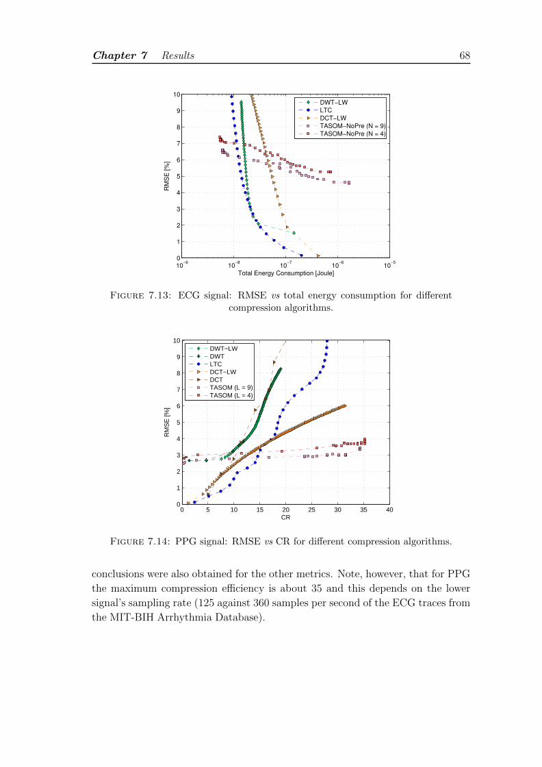
Chapter 7 Results 68
10−9
10−8
10−7
10−6
10−5
0
1
2
3
4
5
6
7
8
9
10
Total Energy Consumption [Joule]
RM
SE
[%
]
DWT−LW
LTC
DCT−LW
TASOM−NoPre (N = 9)
TASOM−NoPre (N = 4)
Figure 7.13: ECG signal: RMSE vs total energy consumption for differentcompression algorithms.
0 5 10 15 20 25 30 35 400
1
2
3
4
5
6
7
8
9
10
CR
RM
SE
[%]
DWT−LWDWTLTCDCT−LWDCTTASOM (L = 9)TASOM (L = 4)
Figure 7.14: PPG signal: RMSE vs CR for different compression algorithms.
conclusions were also obtained for the other metrics. Note, however, that for PPG
the maximum compression efficiency is about 35 and this depends on the lower
signal’s sampling rate (125 against 360 samples per second of the ECG traces from
the MIT-BIH Arrhythmia Database).
Chapter 8
Conclusions
In this thesis, I have presented an original lossy compression approach for wear-
able devices. The proposed technique exploits a dictionary-based design philoso-
phy, where the dictionary is learned and adapted at runtime to best represent the
physiological signals of the subject that wears the device. This is attained using
time-adaptive self-organizing maps, which are recent neural network architectures
featuring continuous learning and adaptation capabilities. The algorithm is shown
to outperform popular compression approaches from the literature, doubling the
maximum achievable compression efficiency of previous schemes belonging to the
same class. This allows for a major reduction in the memory size required by con-
tinuous monitoring applications (up to 35- and 70-fold for PPG and ECG signals,
respectively), which entails a decrease of almost two orders of magnitude in the
total energy consumption of the wearable devices. The use of learning maps makes
it possible to achieve fast tuning to new subjects or to changes in the statistical fea-
tures of their signals, while preserving the morphology of the considered biomedical
time series across all subjects and signal types.
69
Bibliography
[1] I. W. Stats, Usage and Population Statistics, 2015. [Online]. Available:
http://www.internetworldstats.com
[2] L. Atzori, A. Iera, and G. Morabito, “The internet of things: A survey,”
Computer Networks, vol. 54, no. 15, pp. 2787 – 2805, 2010.
[3] J. Gubbi, R. Buyya, S. Marusic, and M. Palaniswami, “Internet of things
(IoT): A vision, architectural elements, and future directions,” Future Gener-
ation Computer Systems, vol. 29, no. 7, pp. 1645–1660, 2013.
[4] K. Finkenzeller, RFID Handbook. John Wiley & Sons, 2003.
[5] M. Zorzi, A. Gluhak, S. Lange, and A. Bassi, “From today’s INTRAnet of
things to a future INTERnet of things: a wireless- and mobility-related view,”
Wireless Communications, IEEE, vol. 17, no. 6, pp. 44–51, 2010.
[6] M. Srivastava, T. Abdelzaher, and B. Szymanski, “Human-centric sensing,”
Philosophical Transactions of the Royal Society of London A: Mathematical,
Physical and Engineering Sciences, vol. 370, no. 1958, pp. 176–197, 2012.
[7] J. Williamson, Q. Liu, F. Lu, W. Mohrman, K. Li, R. Dick, and L. Shang,
“Data sensing and analysis: Challenges for wearables,” in Design Automation
Conference (ASP-DAC), 2015 20th Asia and South Pacific, Jan 2015, pp.
136–141.
[8] IDTechEx, Wearable Technology 2015-2025: Technologies, Markets, Forecasts,
2015. [Online]. Available: http://www.idtechex.com
[9] A. Darwish and A. E. Hassanien, “Wearable and implantable wireless sensor
network solutions for healthcare monitoring,” Sensors, vol. 11, no. 6, pp. 5561–
5595, 2011.
[10] T. Schoellhammer, B. Greenstein, E. Osterweil, M. Wimbrow, and D. Estrin,
“Lightweight temporal compression of microclimate datasets,” in Local Com-
puter Networks, 2004. 29th Annual IEEE International Conference on, Nov
2004, pp. 516–524.
70
Bibliography 71
[11] J. R. Cox, F. M. Nolle, H. A. Fozzard, and G. C. Oliver, “Aztec, a preprocessing
program for real-time ecg rhythm analysis,” Biomedical Engineering, IEEE
Transactions on, vol. BME-15, no. 2, pp. 128–129, April 1968.
[12] J. P. Abenstein and W. J. Tompkins, “A new data-reduction algorithm for
real-time ecg analysis,” Biomedical Engineering, IEEE Transactions on, vol.
BME-29, no. 1, pp. 43–48, Jan 1982.
[13] S. Jalaleddine, C. Hutchens, R. Strattan, and W. Coberly, “Ecg data compres-
sion techniques - a unified approach,” Biomedical Engineering, IEEE Trans-
actions on, vol. 37, no. 4, pp. 329–343, April 1990.
[14] B. Reddy and I. Murthy, “Ecg data compression using fourier descriptors,”
Biomedical Engineering, IEEE Transactions on, no. 4, pp. 428–434, 1986.
[15] H. Lee and K. M. Buckley, “Ecg data compression using cut and align beats
approach and 2-d transforms,” Biomedical Engineering, IEEE Transactions
on, vol. 46, no. 5, pp. 556–564, 1999.
[16] B. Rajoub et al., “An efficient coding algorithm for the compression of ecg
signals using the wavelet transform,” Biomedical Engineering, IEEE Trans-
actions on, vol. 49, no. 4, pp. 355–362, 2002.
[17] D. Zordan, B. Martinez, I. Vilajosana, and M. Rossi, “On the performance of
lossy compression schemes for energy constrained sensor networking,” ACM
Transactions on Sensor Networks (TOSN), vol. 11, no. 1, p. 15, 2014.
[18] A. Iwata, Y. Nagasaka, and N. Suzumura, “Data compression of the ecg us-
ing neural network for digital holter monitor,” Engineering in Medicine and
Biology Magazine, IEEE, vol. 9, no. 3, pp. 53–57, Sept 1990.
[19] C.-C. Sun and S.-C. Tai, “Beat-based ecg compression using gain-shape vector
quantization,” Biomedical Engineering, IEEE Transactions on, vol. 52, no. 11,
pp. 1882–1888, 2005.
[20] J. L. Cardenas-Barrera and J. V. Lorenzo-Ginori, “Mean-shape vector quan-
tizer for ecg signal compression,” Biomedical Engineering, IEEE Transactions
on, vol. 46, no. 1, pp. 62–70, 1999.
[21] N. Maglaveras, T. Stamkopoulos, K. Diamantaras, C. Pappas, and
M. Strintzis, “Ecg pattern recognition and classification using non-linear trans-
formations and neural networks: a review,” International journal of medical
informatics, vol. 52, no. 1, pp. 191–208, 1998.
[22] K. Reddy, B. George, and V. Kumar, “Use of fourier series analysis for motion
artifact reduction and data compression of photoplethysmographic signals,”
Bibliography 72
Instrumentation and Measurement, IEEE Transactions on, vol. 58, no. 5, pp.
1706–1711, May 2009.
[23] Y. Linde, A. Buzo, and R. M. Gray, “An algorithm for vector quantizer design,”
Communications, IEEE Transactions on, vol. 28, no. 1, pp. 84–95, 1980.
[24] J.-J. Wei, C.-J. Chang, N.-K. Chou, and G.-J. Jan, “Ecg data compression
using truncated singular value decomposition,” Information Technology in
Biomedicine, IEEE Transactions on, vol. 5, no. 4, pp. 290–299, Dec 2001.
[25] A. Ramakrishnan and S. Saha, “Ecg compression by multirate processing of
beats,” Computers and biomedical research, vol. 29, no. 5, pp. 407–417, 1996.
[26] S.-G. Miaou and J.-H. Larn, “Adaptive vector quantisation for electrocardio-
gram signal compression using overlapped and linearly shifted codevectors,”
Medical and Biological Engineering and Computing, vol. 38, no. 5, pp. 547–
552, 2000.
[27] D. D. Testa and M. Rossi, “Lightweight lossy compression of biometric pat-
terns via denoising autoencoders,” IEEE Signal Processing Letters, Accepted
for publication.
[28] A. Chatterjee, A. Nait-Ali, and P. Siarry, “An input-delay neural-network-
based approach for piecewise ecg signal compression,” IEEE transactions on
biomedical engineering, vol. 52, no. 5, pp. 945–947, 2005.
[29] J. L. E. K. S. Lonardi and P. Patel, “Finding motifs in time series,” in Proc.
of the 2nd Workshop on Temporal Data Mining, 2002, pp. 53–68.
[30] J. Pan and W. J. Tompkins, “A real-time qrs detection algorithm,” Biomedical
Engineering, IEEE Transactions on, vol. BME-32, no. 3, pp. 230–236, March
1985.
[31] M. Elgendi, “Fast qrs detection with an optimized knowledge-based method:
Evaluation on 11 standard ecg databases,” PloS one, vol. 8, no. 9, p. 73557,
2013.
[32] A. Gersho and R. M. Gray, Vector quantization and signal compression.
Springer Science & Business Media, 2012, vol. 159.
[33] K.-S. Wu and J.-C. Lin, “Fast vq encoding by an efficient kick-out condition,”
Circuits and Systems for Video Technology, IEEE Transactions on, vol. 10,
no. 1, pp. 59–62, 2000.
[34] S. S. Skiena, The algorithm design manual. Springer Science & Business
Media, 1998, vol. 1.
[35] S. Haykin, Neural Networks and Learning Machines. Prentice Hall, 2009.
Bibliography 73
[36] D. M. Miller, E. J. Kaminsky, and S. Rana, “Neural network classification of
remote-sensing data,” Computers and Geosciences, vol. 21, no. 3, pp. 377 –
386, 1995.
[37] K. Hornik, “Some new results on neural network approximation,” Neural Net-
works, vol. 6, no. 8, pp. 1069 – 1072, 1993.
[38] S. Lawrence, C. Giles, A. C. Tsoi, and A. Back, “Face recognition: a convo-
lutional neural-network approach,” Neural Networks, IEEE Transactions on,
vol. 8, no. 1, pp. 98–113, 1997.
[39] G. E. Dahl, D. Yu, L. Deng, and A. Acero, “Context-dependent pre-trained
deep neural networks for large-vocabulary speech recognition,” Audio, Speech,
and Language Processing, IEEE Transactions on, vol. 20, no. 1, pp. 30–42,
2012.
[40] J. Eggermont, The Correlative Brain: Theory and Experiment in Neural In-
teraction, ser. Studies of brain function. Springer-Verlag, 1990.
[41] P. S. Churchland and T. J. Sejnowski, The computational brain. The MIT
press, 1992.
[42] R. Stufflebeam, “Neurons, synapses, action potentials, and neurotransmis-
sion,” Consortium on Cognitive Science Instruction, 2008.
[43] W. McCulloch and W. Pitts, “A logical calculus of the ideas immanent in
nervous activity,” The bulletin of mathematical biophysics, vol. 5, no. 4, pp.
115–133, 1943.
[44] F. Rosenblatt, “The perceptron: a probabilistic model for information storage
and organization in the brain.” Psychological review, vol. 65, no. 6, p. 386,
1958.
[45] D. E. Rumelhart, G. E. Hinton, and R. J. Williams, “Learning representations
by back-propagating errors,” Cognitive modeling, vol. 5, p. 3, 1988.
[46] A. Robinson and F. Fallside, The utility driven dynamic error propagation
network. University of Cambridge Department of Engineering, 1987.
[47] M. A. Fischler and O. Firschein, “Intelligence: the eye, the brain, and the
computer,” 1987.
[48] G. S. Stent, “A physiological mechanism for hebb’s postulate of learning,”
Proceedings of the National Academy of Sciences, vol. 70, no. 4, pp. 997–1001,
1973.
Bibliography 74
[49] J.-P. Changeux and A. Danchin, “Selective stabilisation of developing synapses
as a mechanism for the specification of neuronal networks,” Neurobiology of
Learning and Memory, vol. 2, p. 229, 1990.
[50] T. H. Brown, E. W. Kairiss, and C. L. Keenan, “Hebbian synapses: biophysical
mechanisms and algorithms,” Annual review of neuroscience, vol. 13, no. 1,
pp. 475–511, 1990.
[51] Z. Chen, S. Haykin, J. J. Eggermont, and S. Becker, Correlative learning: a
basis for brain and adaptive systems. John Wiley & Sons, 2008, vol. 49.
[52] E. Oja, “Simplified neuron model as a principal component analyzer,” Journal
of mathematical biology, vol. 15, no. 3, pp. 267–273, 1982.
[53] D. E. Rumelhart and D. Zipser, “Feature discovery by competitive learning,”
Cognitive science, vol. 9, no. 1, pp. 75–112, 1985.
[54] T. Kohonen, “The self-organizing map,” Proceedings of the IEEE, vol. 78,
no. 9, pp. 1464–1480, 1990.
[55] E. I. Knudsen, S. Lac, and S. D. Esterly, “Computational maps in the brain,”
Annual Review of Neuroscience, vol. 10, no. 1, pp. 41–65, 1987.
[56] T. Kohonen, Self-organization and Associative Memory: 3rd Edition. New
York, NY, USA: Springer-Verlag New York, Inc., 1989.
[57] H. Shah-Hosseini and R. Safabakhsh, “Tasom: a new time adaptive self-
organizing map,” Systems, Man, and Cybernetics, Part B: Cybernetics, IEEE
Transactions on, vol. 33, no. 2, pp. 271–282, 2003.
[58] PhysioNet. [Online]. Available: http://www.physionet.org/
[59] ARM, Technical Reference Manual, 2010.
[60] Cortex-M4 Processor Specification. [Online]. Available: http://www.arm.
com/products/processors/cortex-m/cortex-m4-processor.php
[61] S. Kamath and J. Lindh, “Measuring bluetooth low energy power consump-
tion,” Texas instruments application note AN092, Dallas, 2010.


![Lez 14 Fourier [modalit compatibilit ]misure.mecc.polimi.it/files/Materiale Didattico/Lez_15_Fourier.pdf · Grandezza fisica Segnale Trasduttore Segnale ... Quando serve Fourier:](https://img.pdfslide.net/doc/110x75/5c69b6ea09d3f20c178b7c08/lez-14-fourier-modalit-compatibilit-didatticolez15fourierpdf-grandezza.jpg)