Embed Size (px)
Citation preview

Biometrical Tools for Heterosis
Research
Dissertation zur Erlangung des Doktorgrades der
Naturwissenschaften (Dr. rer. nat.)
Fakultät Naturwissenschaften
Universität Hohenheim
Institut für angewandte Mathematik und Statistik
Institut für Kulturpflanzenwissenschaften
vorgelegt von
André Schützenmeister
aus Zeitz
2010

Dekan bzw. Dekanin: Prof. Dr. Heinz Breer
1. berichtende Person: Prof. Dr. Hans-Peter Piepho
2. berichtende Person: Prof. Dr. Uwe Jensen
Eingereicht am: 22.12.2010
Mündliche Prüfung am: 27.05.2011
Die vorliegende Arbeit wurde am 04.04.2011 von der Fakultät Naturwissenschaften der
Universität Hohenheim als „Dissertation zur Erlangung des Doktorgrades der
Naturwissenschaften“ angenommen.

Danksagung
Die vorliegende Dissertation ist während meiner Arbeit an der Universität Hohenheim
entstanden, welche in dem Schwerpunktprogramm Heterosis in Pflanzen (SPP 1149)
der Deutschen Forschungsgemeinschaft (DFG) eingebettet war.
An erster Stelle möchte ich Prof. Dr. Hans-Peter Piepho für die hervorragende Be-
treuung danken. Zum einen gab er mir viel Freiraum, auch eigenen Ideen nachzugehen,
zum anderen nahm er sich immer die Zeit, mir mit Rat und Tat beizustehen wenn seine
Hilfe gefragt war. Ich bin ihm besonders dankbar für seine konstruktive Kritik, welche
mich und meine Arbeit vorangebracht hat und für seine Ausdauer beim Korrekturlesen.
Prof. Dr. Uwe Jensen erklärte sich sofort bereit, meine Betreuung an der Fakultät Na-
turwissenschaften zu übernehmen und war stets ansprechbar, wenn es galt, inhaltliche
sowie organisatorische Fragen zeitnah und kompetent zu beantworten, vielen Dank
dafür.
Außerdem möchte ich meinen Kollegen des FG Bioinformatik am Institut für Kul-
turpflanzenwissenschaften danken, mit denen ich immer rechnen konnte, wenn es
darum ging, ein Manuskript kritisch auf inhaltliche oder stilistische Mängel hin zu
überprüfen. Vor allem möchte ich Bettina Müller und Torben Schulz-Streeck meinen
Dank ausprechen. Generell war die Arbeitsatmosphäre im FG Bioinformatik immer
positiv und motivierend, wozu auch die regelmäßigen gemeinsamen Unternehmungen
beigetragen haben.
Diese Dissertation wäre niemals ohne die Kooperationpartner des SPP 1149 mög-
i

lich gewesen. Insbesonders gilt mein Dank Prof. Dr. Frank Hochholdinger und seiner
Arbeitsgruppe von der Universität Tübingen (jetzt Universität Bonn) sowie Dr. Lilla
Römisch-Margl von der Technischen Universität München. Die gemeinsamen Projekte
haben eine Vielzahl von interessanten Fragestellungen aufgeworfen, welche den Kern
dieser Dissertation bilden.
Weiterhin möchte ich mich bei Prof. Dr. Andreas Schaller für die Vermittlung des Self-
vs-Self Datensatzes bedanken, den mir freundlicherweise Caroline Gouhier-Darimont
und Dr. Philippe Reymond von der Universität Lausanne zur Verfügung gestellt haben.
Abschließend möchte ich meinen Eltern danken, die es mir überhaupt erst ermög-
licht haben, soweit zu kommen, und natürlich meinem Bruder Axel, der mir stets ein
Vorbild gewesen ist und immer für die nötige Motivation gesorgt hat. Vielen Dank liebe
Alida dafür, dass du immer an mich geglaubt hast und mich durch alle Höhen und
Tiefen der letzten Jahre begleitet hast.
André Schützenmeister Hohenheim, Dezember 2010
ii

Contents
Summary 1
Zusammenfassung 3
1 General Introduction 5
1.1 Heterosis . . . . . . . . . . . . . . . . . . . . . . . . . . . . . . . . . . . . . . . . . . . . . . . 5
1.2 Computing and Testing Heterosis Effects . . . . . . . . . . . . . . . . . . . . . . . . 7
1.3 Checking Model Assumptions . . . . . . . . . . . . . . . . . . . . . . . . . . . . . . . . 11
1.4 Two-Color cDNA Microarrays . . . . . . . . . . . . . . . . . . . . . . . . . . . . . . . . 12
1.5 Objectives . . . . . . . . . . . . . . . . . . . . . . . . . . . . . . . . . . . . . . . . . . . . . . 15
2 Residual Analysis for Linear Models 17
2.1 Introduction . . . . . . . . . . . . . . . . . . . . . . . . . . . . . . . . . . . . . . . . . . . . . 17
2.2 Motivating Example . . . . . . . . . . . . . . . . . . . . . . . . . . . . . . . . . . . . . . . 19
2.3 Outline of Approach of Model Checking . . . . . . . . . . . . . . . . . . . . . . . . . 21
2.3.1 Residuals . . . . . . . . . . . . . . . . . . . . . . . . . . . . . . . . . . . . . . . . . . 21
2.3.2 Graphical Methods . . . . . . . . . . . . . . . . . . . . . . . . . . . . . . . . . . . 24
2.3.3 Computing the Monte Carlo p -value . . . . . . . . . . . . . . . . . . . . . . 25
2.4 Checking Normality . . . . . . . . . . . . . . . . . . . . . . . . . . . . . . . . . . . . . . . 26
2.4.1 A Quantile-based Algorithm . . . . . . . . . . . . . . . . . . . . . . . . . . . . 26
2.4.2 A Monte Carlo Test for Normality . . . . . . . . . . . . . . . . . . . . . . . . 28
2.4.3 An Alternative: Orthogonal Residuals . . . . . . . . . . . . . . . . . . . . . 29
2.4.4 Simulation Study . . . . . . . . . . . . . . . . . . . . . . . . . . . . . . . . . . . . 31
2.5 Homoscedasticity and Outliers . . . . . . . . . . . . . . . . . . . . . . . . . . . . . . . 39
2.5.1 Simultaneous Tolerance Limits . . . . . . . . . . . . . . . . . . . . . . . . . . 39
2.5.2 Monte Carlo Tests for Homoscedasticity . . . . . . . . . . . . . . . . . . . 43
iii

3 Residual Analysis for Linear Mixed Models 45
3.1 Introduction . . . . . . . . . . . . . . . . . . . . . . . . . . . . . . . . . . . . . . . . . . . . . 45
3.2 Motivating Example . . . . . . . . . . . . . . . . . . . . . . . . . . . . . . . . . . . . . . . 48
3.3 Linear Mixed Model Residuals . . . . . . . . . . . . . . . . . . . . . . . . . . . . . . . . 50
3.4 The Simulation Approach . . . . . . . . . . . . . . . . . . . . . . . . . . . . . . . . . . . 54
3.5 A Rank-based Algorithm . . . . . . . . . . . . . . . . . . . . . . . . . . . . . . . . . . . . 56
3.6 Examples . . . . . . . . . . . . . . . . . . . . . . . . . . . . . . . . . . . . . . . . . . . . . . . 57
3.6.1 Toothbrush Data . . . . . . . . . . . . . . . . . . . . . . . . . . . . . . . . . . . . 57
3.6.2 Cambridge Filter Data . . . . . . . . . . . . . . . . . . . . . . . . . . . . . . . . 60
3.6.3 Orthodont Data . . . . . . . . . . . . . . . . . . . . . . . . . . . . . . . . . . . . . 64
3.7 Simulation Study . . . . . . . . . . . . . . . . . . . . . . . . . . . . . . . . . . . . . . . . . 68
4 Two-Color cDNA-Microarrays 72
4.1 Introduction . . . . . . . . . . . . . . . . . . . . . . . . . . . . . . . . . . . . . . . . . . . . . 72
4.2 Material and Methods . . . . . . . . . . . . . . . . . . . . . . . . . . . . . . . . . . . . . . 76
4.2.1 Semivariograms . . . . . . . . . . . . . . . . . . . . . . . . . . . . . . . . . . . . . 76
4.2.2 Anisotropy . . . . . . . . . . . . . . . . . . . . . . . . . . . . . . . . . . . . . . . . . 78
4.2.3 Ordinary Kriging . . . . . . . . . . . . . . . . . . . . . . . . . . . . . . . . . . . . 79
4.2.4 Global Trend . . . . . . . . . . . . . . . . . . . . . . . . . . . . . . . . . . . . . . . 80
4.2.5 Model Selection and Estimation . . . . . . . . . . . . . . . . . . . . . . . . . 81
4.3 Three Approaches to BG-Smoothing . . . . . . . . . . . . . . . . . . . . . . . . . . . 87
4.4 Background Correction Methods . . . . . . . . . . . . . . . . . . . . . . . . . . . . . . 89
4.5 Self-versus-Self Data . . . . . . . . . . . . . . . . . . . . . . . . . . . . . . . . . . . . . . . 90
4.6 Computing Pair-wise Linear Contrasts . . . . . . . . . . . . . . . . . . . . . . . . . . 92
4.7 Implementation . . . . . . . . . . . . . . . . . . . . . . . . . . . . . . . . . . . . . . . . . . 93
4.8 Results . . . . . . . . . . . . . . . . . . . . . . . . . . . . . . . . . . . . . . . . . . . . . . . . . 94
5 General Discussion 101
5.1 The Monte Carlo Approach . . . . . . . . . . . . . . . . . . . . . . . . . . . . . . . . . . 101
5.2 Smoothing Background Intensities . . . . . . . . . . . . . . . . . . . . . . . . . . . . 107
5.3 Concluding Remarks . . . . . . . . . . . . . . . . . . . . . . . . . . . . . . . . . . . . . . . 110
References 112
iv

List of Abbreviations
AD . . . . . . . . . . . . . . . . . . . . Anderson-Darling (Test)
ANCOVA . . . . . . . . . . . . . . Analysis of Covariance
ANOVA . . . . . . . . . . . . . . . Analysis of Variance
BG . . . . . . . . . . . . . . . . . . . . Background (Fluorescence Signal)
BGC . . . . . . . . . . . . . . . . . . BG Correction
BLUE . . . . . . . . . . . . . . . . . Best Linear Unbiased Estimator
BLUP . . . . . . . . . . . . . . . . . Best Linear Unbiased Predictor
BLUS . . . . . . . . . . . . . . . . . Best Linear Unbiased Scalar (Residuals)
BPH . . . . . . . . . . . . . . . . . . Best-Parent Heterosis
BS . . . . . . . . . . . . . . . . . . . . BG Subtraction
cBLUS . . . . . . . . . . . . . . . . Close to BLUS (Residuals)
CCD . . . . . . . . . . . . . . . . . . Charge-Coupled Device
cDNA . . . . . . . . . . . . . . . . . Coding DNA
CR . . . . . . . . . . . . . . . . . . . . Conditional Residuals (in LMMs)
CVM . . . . . . . . . . . . . . . . . . Cramer-von Mises (Test)
dCTP . . . . . . . . . . . . . . . . . Deoxycytidine Triphosphate
DE . . . . . . . . . . . . . . . . . . . . Differential Expression/Differentially Expressed (Genes)
DF . . . . . . . . . . . . . . . . . . . . Degrees of Freedom
DNA . . . . . . . . . . . . . . . . . . Desoxyribonucleic Acid
EBLUP . . . . . . . . . . . . . . . . Empirical BLUP
EP . . . . . . . . . . . . . . . . . . . . Empirical Power
ERR . . . . . . . . . . . . . . . . . . . Empirical Rejection Rate
ES . . . . . . . . . . . . . . . . . . . . Empirical Size
FC . . . . . . . . . . . . . . . . . . . . Fold Change (Amount of Differential Expression)
FG . . . . . . . . . . . . . . . . . . . . Foreground (Fluorescence Signal)
i.i.d. . . . . . . . . . . . . . . . . . . Independent and Identically Distributed
LKS . . . . . . . . . . . . . . . . . . . Lilliefors-Kolmogorov-Smirnov (Test)
v

LM . . . . . . . . . . . . . . . . . . . . Linear Model
LMM . . . . . . . . . . . . . . . . . Linear Mixed Model
LOWESS . . . . . . . . . . . . . . Locally Weighted Regression
LUS . . . . . . . . . . . . . . . . . . . Linear Unbiased Scalar (Residuals)
MC . . . . . . . . . . . . . . . . . . . Monte Carlo
ML . . . . . . . . . . . . . . . . . . . . Maximum Likelihood
MPH . . . . . . . . . . . . . . . . . . Mid-Parent Heterosis
mRNA . . . . . . . . . . . . . . . . Messenger RNA
OK . . . . . . . . . . . . . . . . . . . . Ordinary Kriging
OLS . . . . . . . . . . . . . . . . . . . Ordinary Least Squares (Estimation)
OR . . . . . . . . . . . . . . . . . . . . Orthogonal Residuals
PCR . . . . . . . . . . . . . . . . . . . Polymerase Chain Reaction
PCS . . . . . . . . . . . . . . . . . . . Pearson Chi-Squared (Test)
QQ-plot . . . . . . . . . . . . . . . Quantile-Quantile Plot
REML . . . . . . . . . . . . . . . . . Restricted Maximum Likelihood
RNA . . . . . . . . . . . . . . . . . . Ribonucleic Acid
RSS . . . . . . . . . . . . . . . . . . . Residual Sum of Squares
SF . . . . . . . . . . . . . . . . . . . . . Shapiro-Francia (Test)
STB . . . . . . . . . . . . . . . . . . . Simultaneous Tolerance Band
STI . . . . . . . . . . . . . . . . . . . . Simultaneous Tolerance Interval
SVS . . . . . . . . . . . . . . . . . . . Self vs. Self (Data)
SW . . . . . . . . . . . . . . . . . . . . Shapiro-Wilk (Test)
TB . . . . . . . . . . . . . . . . . . . . Tolerance Band
TI . . . . . . . . . . . . . . . . . . . . . Tolerance Interval
VSOM . . . . . . . . . . . . . . . . . Variance Shift Outlier Model
VSV . . . . . . . . . . . . . . . . . . . Variance of Semivariances
WLS . . . . . . . . . . . . . . . . . . Weighted Least Squares (Estimation)
vi

Summary
Molecular biological technologies are frequently applied for heterosis research. Large
datasets are generated, which are usually analyzed with linear models or linear mixed
models. Both types of model make a number of assumptions, and it is important to
ensure that the underlying theory applies for datasets at hand. Simultaneous viola-
tion of the normality and homoscedasticity assumptions in the linear model setup can
produce highly misleading results of associated t - and F -tests. Linear mixed models
assume multivariate normality of random effects and errors. These distributional as-
sumptions enable (restricted) maximum likelihood based procedures for estimating
variance components. Violations of these assumptions lead to results, which are un-
reliable and, thus, are potentially misleading. A simulation-based approach for the
residual analysis of linear models is introduced, which is extended to linear mixed
models. Based on simulation results, the concept of simultaneous tolerance bounds is
developed, which facilitates assessing various diagnostic plots. This is exemplified by
applying the approach to the residual analysis of different datasets, comparing results
to those of other authors. It is shown that the approach is also beneficial, when applied
to formal significance tests, which may be used for assessing model assumptions as
well. This is supported by the results of a simulation study, where various alternative,
non-normal distributions were used for generating data of various experimental designs
of varying complexity. For linear mixed models, where studentized residuals are not
pivotal quantities, as is the case for linear models, a simulation study is employed for
1

assessing whether the nominal error rate under the null hypothesis complies with the
expected nominal error rate.
Furthermore, a novel step within the preprocessing pipeline of two-color cDNA
microarray data is introduced. The additional step comprises spatial smoothing of
microarray background intensities. It is investigated whether anisotropic correlation
models need to be employed or isotropic models are sufficient. A self-versus-self
dataset with superimposed sets of simulated, differentially expressed genes is used to
demonstrate several beneficial features of background smoothing. In combination with
background correction algorithms, which avoid negative intensities and which have
already been shown to be superior, this additional step increases the power in finding
differentially expressed genes, lowers the number of false positive results, and increases
the accuracy of estimated fold changes.
2

Zusammenfassung
Molekularbiologische Verfahren werden häufig in der Heterosis-Forschung eingesetzt.
Dabei werden große Datensätze generiert, welche gewöhnlich mittels linearer oder
linearer gemischter Modelle analysiert werden. Beide Modellklassen setzen bestimmte
Annahmen voraus, damit deren zugrunde liegende Theorie greift. Werden die Annah-
men der Normalität und Varianzhomogenität für lineare Modelle gleichzeitig verletzt,
kann das zu völlig falschen Ergebnissen bei den zugehörigen t - und F -Tests führen. Bei
linearen gemischten Modellen wird multivariate Normalverteilung der zufälligen Effek-
te sowie der Fehlerterme vorausgesetzt. Diese Verteilungsannahmen ermöglichen die
Anwendung des (Restricted) Maximum Likelihood Verfahrens zur Schätzung der Vari-
anzkomponenten. Verletzung dieser Annahmen führen zu ungenauen Schätzungen und
sind deshalb von geringem Nutzen. Es wird ein auf Simulation beruhendes Verfahren für
die Residuenanalyse linearer Modelle vorgestellt, welches dann auf lineare gemischte
Modelle erweitert wird. Basierend auf den simulierten Daten wird das Konzept simulta-
ner Toleranzgrenzen entwickelt, welches die Bewertung verschiedener diagnostischer
Plots vereinfacht. Dies wird anhand der jeweiligen Residuenanalyse für verschiedene
Datensätze gezeigt, wobei die Ergebnisse des auf Simulation beruhenden Verfahrens
mit denen anderer Autoren verglichen werden. Außerdem wird gezeigt, dass dieses
Verfahren auf Signifikanztests, welche man ebenfalls zur Überprüfung der Modellvor-
aussetzungen benutzen könnte, übertragen werden kann und dabei von Vorteil ist. Die
Ergebnisse einer Simulationsstudie lassen dies erkennen, wobei verschiedene alternati-
3

ve Verteilungen benutzt werden, um Daten verschiedener, unterschiedlich komplexer
Designs zu erzeugen. Im Falle von linearen gemischten Modellen sind studentisierte
Residuen nicht unabhängig von Modellparametern, was bei linearen Modellen der Fall
ist. Aus diesem Grund wird eine Simulationsstudie präsentiert, welche die Fragestellung
klären soll, ob die empirischen Fehlerraten von simultanen Toleranzgrenzen von den
erwarteten Fehlerraten abweichen, wenn man Daten unter der Nullhypothese simuliert.
Desweiteren wird ein Verfahren für die komplexe Preprozessierung von 2-Kanal
cDNA Microarrays vorgestellt. Dieser zusätzliche Schritt umfasst räumliche Glättungs-
verfahren für die Hintergrundfluoreszens von Microarrays. Es wird der Frage nachge-
gangen, ob man Verfahren benötigt, welche anisotrope Korrelationsmodelle verwenden,
oder ob isotrope Modelle ausreichen. Um die verschiedenen vorteilhaften Eigenschaf-
ten dieses Verfahrens zu zeigen, wird ein Self-versus-Self Microarray Datensatz mit
einem simulierten Anteil differentiell exprimierter Gene verwendet. Kombiniert man
Verfahren zur Glättung der Hintergrundwerte mit etablierten Verfahren zur Hintergrund-
korrektur, welche negative Spot-Intensitäten vermeiden, kann eine höhere statistische
Power beim Nachweis differentiell exprimierter Gene erzielt werden. Außerdem kann
der Anteil falsch-positiver Ergebnisse reduziert und die Präzision der Quantifizierung
von differentieller Expression erhöht werden.
4

Chapter 1
General Introduction
1.1 Heterosis
Gregor Mendel discovered the basic tenets of heredity in the mid-1900s, which are now
known as Mendel’s laws. They explain which phenotypic value of a specific characteris-
tic (trait) could be expected, when crossing two plants with known, distinct genotypes.
Generally, one would expect offspring and parents to be alike, provided that a specific
characteristic is genetically determined. There is one major exception from this rule
- heterosis. It is the scientific term for the phenomenon that crossing of genetically
distinct, homozygous parents (inbred lines) produces highly heterozygous offspring,
so-called hybrids, which can perform significantly better than one would expect from
the mean parental performance (mid-parent value). This principle applies to almost any
quantitative characteristic in the F1 generation. Further selfing of the progeny results in
less heterozygous plants and reduced performance, the so called inbreeding depression
(Becker, 1993).
Heterosis or hybrid vigor has been exploited commercially ever since it was first
scientifically described by Shull (1908) approximately 100 years ago. And it was Shull
who introduced the term heterosis during a lecture given in Göttingen 1917 (Sahrholz,
5

1.1. HETEROSIS 6
2007). In modern plant breeding, exploitation of heterosis is considered as one of the
landmark achievements, which is confirmed by the fact that the acreage under hybrid
cultivars is steadily increasing. This could play a key role in meeting the increasing
needs for food and feed production in the future (Melchinger, 2010).
Although modern plant breeding heavily depends on heterosis, the underlying
molecular mechanisms are still not completely understood. Its paramount agronomic
importance and the lack of fundamental knowledge has attracted many scientists
around the world to investigate the molecular processes governing heterosis. Many
studies focused on the genetic causes of heterosis effects on the level of nucleic acids
(DNA, RNA), which can be summarized as genomics-studies (Beló et al., 2010; Frisch
et al., 2010; Höcker et al., 2008; Jahnke et al., 2010; Thiemann et al., 2010; Uzarowska
et al., 2007, 2009). Others concentrated on heterotic effects for proteins, which fall in
the category of proteomics-studies (e.g. Marcon et al., 2010), and there were studies
performed using metabolomics, i.e. they investigated heterosis in the context of single
metabolites, e.g. sugars, sugar-phosphates, and amino acids (Römisch-Margl et al.,
2010). These three types of studies, all based on molecular biological techniques, are
frequently summarized as omics studies.
This thesis originated from a project within the Deutsche Forschungsgemeinschaft
(DFG) priority program Heterosis in plants (SPP 1149), which was established in order
to study the underlying causes of heterosis. The main task for our group was to analyze
diverse omics datasets, to develop biometrical tools for heterosis research, and to
provide statistical support. The methodology developed in Chapters 2 and 3 is the
result of being faced with different problems concerning model checking and outlier
detection for proteomics and metabolomics data, whereas Chapter 4 was motivated by
the large number of microarray experiments conducted within SPP 1149 (Keller et al.,
2005; Piepho et al., 2006; Uzarowska et al., 2007, 2009; Höcker et al., 2008). Therefore, it
came naturally to have a closer look at all the steps that have to be taken to get from

1.2. COMPUTING AND TESTING HETEROSIS EFFECTS 7
cell material to statistically verified statements based on microarray data. Chapter 4
describes an approach to improve a specific step of the complex preprocessing pipeline,
background correction, which has to be applied to raw cDNA microarray data in order
to remove unwanted non-biological variation (see Sections 1.4 and 4.1).
All studies that explicitly quantify the heterosis effect of a measured characteristic
(gene expression, protein and metabolite abundance, yield, resistance to pathogens)
make use of the appropriate linear contrast and require prior fitting of a statistical model
to collected data. Heterosis contrasts are usually based on fitting either a linear model
(LM) or a linear mixed model (LMM), which is done in an element-wise manner, i.e.
LMs or LMMs are fitted to single genes, proteins, metabolites.
1.2 Computing and Testing Heterosis Effects
In order to define heterosis mathematically, one first needs to define the expected values
of a specific characteristic for parent AA, parent B B , and hybrid A B , denoted as µAA ,
µB B , and µA B , respectively. Then, mid-parent heterosis (MPH) can be defined as
M PH =µA B −µAA +µB B
2. (1.1)
The term MPH indicates that the quantity defined in (1.1) refers to the expected mid-
parent value (mean). There is another type of heterosis, referred to as best-parent
heterosis (BPH). It is BPH, which plant breeders actually aim at, when breeding crops
for improving quantitative characteristics such as yield. It can be defined as
BPH =µA B −max (µAA ,µB B ), (1.2)
where BPH now corresponds to the difference of the hybrid value µA B and the better
of both parental values. Figure 1.1 depicts a sketching of the MPH and BPH effects for
maize.

1.2. COMPUTING AND TESTING HETEROSIS EFFECTS 8
Figure 1.1: Heterosis in maize. The hybrid shows better performance than the mean value ofboth parents, which is referred to as mid-parent heterosis (MPH). In case the hybrid outperformsthe better parent, one speaks of better-parent heterosis (BPH).
Both, (1.1) and (1.2) require estimates µAA , µB B , and µA B , which are usually obtained
from fitting either an LM as used in Chapter 2 or an LMM as used in Chapter 3, depend-
ing on the experimental design, which may require additional fixed or random effects.
In case of a simple LM for a completely randomized design, where the genotype or line
effect is the only fixed effect in the model, the ordinary least squares (OLS) estimate for
genotype i corresponds to the simple arithmetic mean (Searle, 1971)
µi = x i =
∑n i
j=1 x i j
n i, i ∈ {AA, B B , A B} , (1.3)
where n i corresponds to the number of observations for genotype i , n = n AA+n B B+n A B ,
and x i j is the j -th observation of genotype i . In reality, LMs used to estimate genotype
effects are often more complicated, i.e. there are additional fixed effects, which makes
(1.3) inappropriate.

1.2. COMPUTING AND TESTING HETEROSIS EFFECTS 9
The general linear model can be written in standard matrix notation as
y =Xβ + e , (1.4)
where y is the (n × 1) vector of observations, X is the (n × p ) design/model matrix
linking y to the elements of the (p×1) vector of fixed effectsβ , where p = rank (X ). This
assumes that X is of full rank. In an LM, as used for heterosis research, β comprises
genotype effects µAA , µB B , µA B , and any additional parameters. Its OLS-estimator can
be written as
β = (X T X )−1X T y . (1.5)
Genotype effects can than be extracted from the vector of parameter estimates β and
used for the computation of MPH or BPH. This can be done conveniently by estimating
an appropriate linear contrast l Tβ , where l is a (p ×1) vector of coefficients linked to
the p elements of β . The null hypothesis to be tested is
H0 : l Tβ = 0, (1.6)
and a general t -statistic can be constructed
t =l T β
p
l T (X T V −1X )−1l, (1.7)
where V = σ2I , and σ2 is an estimate of residual varianceσ2 (see Section 2.3.1). Then, t
is compared to a t -distribution with (n −p ) degrees of freedom. The use of a t -statistic
directly follows from taking the square-root of the well known Wald-type F -statistic
with one numerator degree of freedom, i.e. l corresponds to a single degree of freedom
hypothesis, whereas the F -statistic can be used for simultaneously testing multiple
hypotheses (Verbeke & Molenberghs, 2000). The MPH (1.1) or BPH (1.2) contrast can
be tested by choosing the appropriate coefficient vector l , where coefficients for all

1.2. COMPUTING AND TESTING HETEROSIS EFFECTS 10
but the three genotype effects are equal to zero. The associated null hypotheses with
appropriate coefficient values can be written as
H0 : 1×µA B −1
2×µAA −
1
2×µB B = 0, (1.8)
and
H0 : 1×µA B −1×max (µAA ,µB B ) = 0. (1.9)
The LMM written in standard matrix notation takes the form
y =Xβ +Z b + e , (1.10)
where y is a (n×1) vector of observations,β is a (p×1)fixed effects parameter vector, b is
a (q×1) vector of random effects, X and Z are (n×p ), respectively, (n×q ) design/model
matrices for β and b , and e is a (n × 1) vector of random error terms. MPH (1.8)
and BPH (1.9) hypotheses can be tested with (1.7), comparing t to the appropriated
t -distribution. Usually, the corresponding degrees of freedom of this t -distribution
have to be approximated (Kenward & Roger, 1997, 2009). Fixed effects are estimated as
β = (X T V −1X )−1X T V −1y , (1.11)
which is the generalized least squares estimator of β . V is an estimate of the variance-
covariance matrix V = (Z G Z T +R ) of y , where G and R are the variance-covariance
matrices of b and e , respectively.
Whenever X does not have full row-column rank, a generalized inverse has to be
used in (1.5), (1.7) and (1.11). It should be kept in mind that using a generalized inverse
results in fixed effect parameter estimates, which cannot be interpreted meaningfully,
because there are infinitely many generalized inverse matrices. However, any estimable
function ofβ is fortunately invariant to the choice of a generalized inverse, and thus, has

1.3. CHECKING MODEL ASSUMPTIONS 11
a meaningful interpretation and can be tested. MPH and BPH contrasts are estimable
(Searle, 1971, p. 161).
1.3 Checking Model Assumptions
Formula (1.7) can be used to infer whether the estimated genotypic effect of the hy-
brid characteristic, which exceeds either the mid-parent value (MPH) or the higher of
both parental estimates (BPH), is statistically significant or not. If so, an experimenter
concludes that a heterosis effect could be verified. This is correct, when model assump-
tions of LMs or LMMs were met, otherwise one cannot assume universal robustness
of the associated t - and F -tests, even for large samples. Bradley (1980, 1984) showed,
that for LMs t -tests and F -tests can be highly misleading in case the normality and
the homoscedasticity assumptions are violated simultaneously, although, both test
statistics are very robust against violation of only a single assumption. For LMMs, the
t -statistic (1.7) assumes normality of the random effects b and of the random errors e .
Thus, inference drawn from testing (1.7) with an appropriate t -distribution depends
on meeting these assumptions. Besides violation of the distributional assumptions,
inference drawn from LMs and LMMs can also be adversely influenced by outlying
observations, e.g. estimated effects of a genotypic characteristic can be severely biased
by outliers. This would directly influence MPH and BPH estimates. Therefore, it is
desirable to detect and remove outliers before drawing any conclusions and to assess
the aforementioned model assumptions.
A popular means for assessing normality and homoscedasticity for LMs (Seber, 1977;
Atkinson, 1985; Draper & Smith, 1998) and LMMs (Lange & Ryan, 1989; Nobre & Singer,
2007; Pinheiro & Bates, 2000) are diagnostic plots. Quantile-quantile (QQ) plots are
frequently used to check the normality of residuals. The ordered vector of residuals
(order statistics) is plotted vs. the expected values of a standard normal distribution.
Larger deviations from the diagonal line indicate possible problems, unfortunately,

1.4. TWO-COLOR CDNA MICROARRAYS 12
without quantifying how severe such deviations are. Another problem with diagnostic
plots is that no human judgment is free of subjectivity. The same diagnostic plot might
be acceptable for one person, while being not acceptable for another person. Therefore,
a lot of experience is required in order to correctly assess QQ-plots. The same problems
apply to other types of diagnostic plots, e.g. to plots of residuals vs. predicted values,
which are particularly useful assessing homoscedasticity or the presence of outlying
observations. There were attempts to add some of the required objectivity. For example,
Atkinson (1981, 1985) proposed point-wise tolerance intervals for each residual point,
so called envelopes. Atkinson used few simulations, which results in erratic bounds of
the envelopes. Furthermore, the envelopes do not consider simultaneous coverage. The
apparent similarities to multiple testing problems are not accounted for, i.e. envelopes
are too narrow and thus too liberal. It would be useful to have visual aids, which provide
some guidance when assessing diagnostic plots. The proposed simultaneous tolerance
bounds described in Chapters 2 and 3 accomplish that.
1.4 Two-Color cDNA Microarrays
As mentioned above, two-color cDNA microarrays are routinely applied for heterosis
research, i.e. heterotic effects are investigated for single genes. The simplest LM for
analyzing microarray data for one gene can be written as
yi j k =αi +βj +γk + e i j k , (1.12)
where yi j k represents the spot intensity for the i -th condition (e.g. genotype) on the
j -th microarray, coming from dye-channel k . To understand this basic model, and
particularly the meaning of the fixed effects in (1.12), one first needs to understand the
functional principle of two-color cDNA microarrays.
A microarray comprises of many spots (103−105), which are microscopic circular

1.4. TWO-COLOR CDNA MICROARRAYS 13
areas with distinct, known locations. Each spot contains many short DNA sequences
(probes), which are immobilized onto the microarray surface. These sequences are
complementary to a specific gene. Gene expression products, so called messenger
RNA1 (mRNA) molecules are isolated from tissue samples and subsequently reverse
transcribed into coding DNA2 (cDNA ), often called targets. Then, samples of two differ-
ent conditions, e.g. genotypes, are labeled with different fluorescence dyes, common
are green (Cy3) and red (Cy5). The labeled cDNAs of both conditions are mixed and put
onto the microarray, where each cDNA molecule can hybridize to its complementary
sequence. Cy3- and Cy5-labeled cDNAs, which correspond to the same gene, bind
competitively to the immobilized sequences at a specific spot. Unbound cDNAs are
washed off, only bound sequences remain on the chip. Red and green fluorophores are
excited to emit light of a specific wavelength using a laser. A CCD3-camera takes a pic-
ture, and the light signals are subsequently transformed into real numbers using special
image analysis software (Mary-Huard et al., 2004; Schena, 2003). The more mRNA of
a specific gene was in the original tissue sample, the higher is the final fluorescence
signal. At each spot two signals are obtained (Cy3, Cy5), and the ratio of both signals is
the so called Fold Change. If this ratio is significantly different from zero, one terms a
gene differentially expressed (DE), and the amount of differential expression is usually
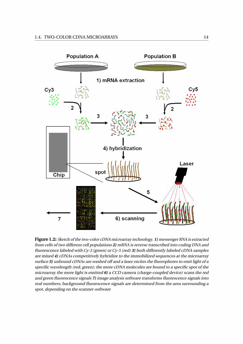
expressed as log2 Fold Change. Figure 1.2 summarizes the steps from a tissue sample to
the final fluorescence signals.
Before drawing inference from fitting a model to gene expression data, e.g. model
(1.12), there are several preprocessing steps required, because any differences among
genotypes may be due to true biological variation or caused by non-biological sources
(see Section 4.1). An experimenter is, of course, only interested in effects that are due to
biological sources. For that reason, many methods were published aiming at filtering
1 Ribonucleic Acid2 Desoxyribonucleic Acid3 Charge Coupled Device
1.4. TWO-COLOR CDNA MICROARRAYS 14
Figure 1.2: Sketch of the two-color cDNA microarray technology. 1) messenger RNA is extractedfrom cells of two different cell populations 2) mRNA is reverse transcribed into coding DNA andfluorescence labeled with Cy-3 (green) or Cy-5 (red) 3) both differently labeled cDNA samplesare mixed 4) cDNAs competitively hybridize to the immobilized sequences at the microarraysurface 5) unbound cDNAs are washed off and a laser excites the fluorophores to emit light of aspecific wavelength (red, green); the more cDNA molecules are bound to a specific spot of themicroarray the more light is emitted 6) a CCD camera (charge-coupled device) scans the redand green fluorescence signals 7) image analysis software transforms fluorescence signals intoreal numbers; background fluorescence signals are determined from the area surrounding aspot, depending on the scanner-software

1.5. OBJECTIVES 15
out the biological signals (Fujita et al., 2006; Haldermans et al., 2007; Huber et al., 2002;
Irizarry et al., 2003; Piepho et al., 2006; Smyth & Speed, 2004; Yang et al., 2002). Once
these signals are obtained, heterosis effects for individual genes can be computed using
LMs and/or LMMs. One particular step of the complex preprocessing pipeline dealing
with a technical source of variation is background (BG) correction. Regularly, labeled
cDNA molecules bind to the glass surface of a microarray outside the spot areas where
no complementary sequences were immobilized. These molecules also emit light when
excited by the laser, and the resulting fluorescence biases the signals of the nearby spots.
Therefore, these so-called BG signals are quantified in the vicinity of each spot, and they
are usually subtracted from the foreground (FG) signals, which has been the standard BG
correction procedure for quite some time (Ritchie et al., 2007; Schena, 2003). Frequently,
however, these BG values exceed the FG values, and hence, their differences FG − BG
become negative, which causes problems when computing log-values. Furthermore,
negative gene expression signals cannot be explained biologically. A solution to this
problem are algorithms, which avoid negative BG corrected signals (Edwards, 2003;
Ritchie et al., 2007). In Chapter 4 an approach to improving BG correction is investigated,
which is based on smoothing BG values.
1.5 Objectives
This thesis comprises of three distinct chapters. Each chapter will be introduced sep-
arately. The developed methodology presented in Chapters 2 - 4 was motivated by,
but is not restricted to heterosis research. Each chapter reflects handling of a specific
difficulty encountered during the participation in SPP 1149. Specifically, Chapters 2
and 3 were motivated by application of linear models (LM) and linear mixed models
(LMM) in proteomics- and metabolomics-studies (Marcon et al., 2010; Römisch-Margl
et al., 2010), while Chapter 4 reflects the importance of preprocessing of microarray
data (Ritchie et al., 2007; Yang et al., 2002; Yin et al., 2005).

1.5. OBJECTIVES 16
Chapter 2 introduces a simulation-based approach to model checking and detection
of outliers applicable for LMs. It is shown how Monte Carlo (MC) procedures can be used
to improve diagnostic plots in terms of minimizing the unavoidable subjectivity involved
assessing these plots. Furthermore, it is shown how MC procedures can be applied to
formal significance tests for normality and variance homogeneity (homoscedasticity),
yielding better power compared to the same tests applied only once to the observed data.
The diagnostic tools developed in Chapter 2 will be applied to a previously published
dataset to demonstrate the usefulness of this approach. Chapter 3 extends this approach
to LMMs. LMMs comprise more than one random term besides the fixed effects, in
contrast to LMs. This results in several types of LMM residuals, which can be defined.
Application to three datasets exemplifies the usefulness of the simulation approach
for LMMs by comparing the results obtained with the simulation approach to those of
other publications.
The approach to BG correction of two-color cDNA microarray data (Chapter 4) orig-
inate from a wealth of microarray datasets, produced from groups participating in SPP
1149 (e.g. Höcker et al., 2008; Jahnke et al., 2010; Uzarowska et al., 2007, 2009). In Chap-
ter 4, it is investigated whether BG correction can be improved, when smoothing BG
values prior to applying established BG correction algorithms. Of special interest was,
to which extend smoothing of BG values improve the ability to detect DE genes. A com-
plex geostatistical framework is developed, capable of differentiating between isotropic
and anisotropic models, which best reflect local BG values. This complex approach is
compared to two simpler methods, which do not consider anisotropy. A self-vs-self
dataset is employed, which does not contain truly DE genes. This enables checking the
empirical error rate under the null hypothesis (empirical size), and additionally, when
DE genes are simulated, the performance of each BG smoothing approach in terms of
power, false classification, and accuracy as will be detailed in Chapter 4.

Chapter 2
Residual Analysis for Linear Models
2.1 Introduction
A common approach to checking assumptions of the general linear model is to com-
pute residuals and either produce various residual plots, or to subject these to tests of
normality and homoscedasticity. These procedures strictly assume that residuals have
the same distributional properties as the true errors, which is always an approximation,
because residuals are linear combinations of the true errors and so are stochastically
dependent and may also be heteroscedastic, e.g. in simple linear regression. Least
squares estimation of linear models with independent and identically distributed (i.i.d.)
errors always results in some non-zero covariances between pairs of residuals. This is a
consequence of having n residuals, which carry only (n-p) degrees of freedom, where n
is the number of observations and p is the rank of the design/model matrix X (Draper
& Smith, 1998, p. 206).
Moreover, the residuals may exhibit supernormality, i.e. the residuals appear to be
more normal than the underlying distribution of errors if this is non-normal (Atkinson,
1985). This characteristic can directly influence the outcome of statistical tests as well
as the interpretation of diagnostic plots for normality or homoscedasticity. Further-
17

2.1. INTRODUCTION 18
more, when interpreting diagnostic plots, there is always an unavoidable element of
subjectivity.
Inference for linear models may be non-robust against violations of both the nor-
mality and homoscedasticity assumptions. Bradley (1980, 1984) showed that even for a
large number of observations the inference drawn from F -tests and t -tests can be mis-
leading when both assumptions are violated simultaneously, although they are usually
robust against violations of only a single assumption in case of a sufficient sample size.
Our approach allows assessing both assumptions simultaneously with the same set of
simulation results.
Exploiting the fact that studentized residuals are pivotal statistics (Dufour et al.,
1998; Cox & Hinkley, 1974, p. 211), the null distribution of a particular set of residuals as
well as the null distribution of any test statistic computed from these residuals can be
simulated. Piepho (1996a) used studentized residuals to construct a simulation-based
test for homoscedasticity within the linear model framework. Dufour et al. (1998) used
the same idea and compared eleven normality tests in terms of size and power with
their Monte Carlo-based counterparts in linear regressions. The authors showed that
the size of these tests is more precisely controlled when p -values are computed by
their Monte Carlo (MC) procedure. In the same vein, Atkinson (1981, 1985) suggests to
compute envelopes in half-normal plots, which are basically simulation-based point-
wise tolerance intervals (TI) for each residual. Plotting these envelopes gives the user a
general idea how severe potential departures from the assumptions are e.g. in QQ-plots.
Atkinson (1981) simulated a rather small number of data vectors (N=19).
In this chapter we propose a simulation-based graphical procedure for checking the
normality and homoscedasticity assumptions, which takes into account that residuals
may be correlated and heteroscedastic even when the underlying assumptions are
met for the errors. We further develop the ideas of Atkinson’s envelopes (Atkinson,
1981, 1985; Atkinson & Riani, 2000) and Piepho’s MC test for variance homogeneity

2.2. MOTIVATING EXAMPLE 19
(Piepho, 1996a). In particular, we show how results of the MC procedure can be used to
construct simultaneous tolerance bounds. These bounds help to interpret diagnostic
plots for normality and homoscedasticity, objectify their interpretation, and also provide
asymptotically valid level-α tests.
This chapter is organized as follows. We start with a small example from metabolite
profiling (Römisch-Margl et al., 2010), which exemplifies the problems an experimenter
faces in interpreting diagnostic plots. Subsequently, the general idea underlying the
Monte Carlo procedures is presented as well as an algorithm for constructing a simul-
taneous tolerance band (STB) for normality. Methods for checking homoscedasticity
and the identification of outlying observations based on our MC procedure will be
introduced. All these methods are exemplified using a previously published dataset.
2.2 Motivating Example
Römisch-Margl et al. (2010) performed extensive measurements of metabolites in the
early stages of the developing maize kernel. They aimed at investigating heterotic
patterns of dry matter, starch, sugars, sugar-phosphates, and free amino acids for the
B73×Mo17 hybrid and its parental lines at six developmental stages (8, 12, 16, 20, 25, 30
days past pollination). We consider the fructose measurements in the whole kernel at
eight days past pollination. Interest was in the differences among genotypes. For this
set-up we use the linear model,
yi j =µ+αi + e i j ,
where yi j is the j -th measured metabolic quantity (j = 1, ..., n i ;n = n 1+n 2+ ...+n k )
of genotype i , (i = 1, ..., k ), µ is the general mean, αi is the effect of the i -th genotype,
e i j ∼N (0,σ2) is the i.i.d. residual error corresponding to yi j . The standard procedure for
checking normality would consist of fitting the model, extracting studentized residuals,

2.2. MOTIVATING EXAMPLE 20
Figure 2.1: (1s t ) : QQ-plot of studentized residuals for the metabolite data described inRömisch-Margl et al. (2010). (2nd ) : The same plot with the point-wise 95% tolerance band(dashed) and Bonferroni-corrected 95% simultaneous tolerance band (dotted).
and constructing a QQ-plot (Figure 2.1, 1s t plot). This plot shows an increasing volatility
toward both ends, and it is not clear whether this is within expectation based on the
properties of order statistics, or indication of real departure from assumptions. In
particular, it is not clear, whether there are any outlying observations. This illustrates
the general problem with QQ-plots for a user in deciding whether the pattern of points
is indicative of departure from normality or not. The same problem occurs with other
residual plots. For this reason, it would be useful to have tolerance bands (TB) such that
a QQ-plot can be judged acceptable whenever all plotted quantiles for the residuals are
inside the band. This idea is similar to the envelopes suggested by Atkinson (1981, 1985)
for half-normal plots. Atkinson only considers control of the point-wise α level. We here
propose to use an STB which has simultaneous coverage probability (1−α).
Our approach is based on the simulation of N datasets, that have the same size (n ),
the same correlation structure, and the same design/model matrix X as the observed
data. For each simulated dataset we compute residuals and order them by size. For
the i -th order statistic there are N simulated residuals. Among these, we compute the
(α/2) and (1−α/2) quantiles to obtain a (1−α)100% tolerance interval. These quantiles

2.3. OUTLINE OF APPROACH OF MODEL CHECKING 21
are denoted here as local. If N →∞, the local interval attains exact coverage. Note,
however, that it controls only the point-wise coverage probability, not the simultaneous
coverage probability (see Figure 2.1, 2nd plot, dashed lines). To account for multiplicity,
bounds of these intervals could be corrected e.g. by Bonferroni adjustment where
instead of the (α/2) and (1−α/2) quantiles of the i-th order statistic the (α/2n) and
(1−α/2n ) quantiles are used, respectively. Bonferroni adjustment guarantees that the
simultaneous coverage probability is greater than or equal to (1−α). By the Bonferroni
method, each local error level γ is assigned the same value γ= α/n , which results in
the characteristic form of the STB familiar from regression. An example is shown in
Figure 2.1 (2nd plot, dotted lines). The Bonferroni method is known to be conservative,
while the point-wise (1−α) TB is too liberal. Some improvement is therefore desirable.
Specifically, an improved procedure to compute more narrow STBs compared to the
Bonferroni method is required, that accounts for dependencies among residuals. Our
proposed method accomplishes that.
2.3 Outline of Approach of Model Checking
2.3.1 Residuals
The general linear model, written in standard matrix notation, has the form
y =Xβ + e , (2.1)
where y is the vector of observed values, β is a vector of fixed effects, X is the de-
sign/model matrix which corresponds to β , and e is a vector of residual errors. The
null hypothesis to be tested is that e ∼ N (0,σ2I ), which is one prerequisite for stan-
dard analysis by the general linear model. Departure from this assumption may hint
at outlying observations which should be removed prior to analysis, or there may be

2.3. OUTLINE OF APPROACH OF MODEL CHECKING 22
heteroscedasticity or non-normality of e , which might be avoided by a suitable data
transformation.
Our proposed Monte Carlo procedure makes use of the ordinary least squares (OLS)
residuals e = (I −H )y , where H =X (X T X )−1X T (hat matrix), which are free of param-
eters β . To see this, consider a random vector y = Xβ + zσ, where z is a vector of
independent standard normal deviates. Vector y has expectation Xβ with variance-
covariance matrixσ2I . The OLS residuals are:
e = (I −X (X T X )−1X T )y (2.2)
and therefore
e = (I −X (X T X )−1X T )(Xβ + zσ) (2.3)
and
e =σ(I −X (X T X )−1X T )z , (2.4)
which is free of β , since X − X (X T X )−1X T X = 0 (Searle, 1971, p. 20). Studentized
residuals are computed by
e i =e i
σp
1−h i i
, i = 1, ..., n (2.5)
where h i i is the i-th diagonal element of H and
σ2 =y T (I −H )y
n −p=
e T e
n −p, (2.6)
where p = rank (X ). The expression σp
1−h i i is the i -th diagonal element of the
estimate of the variance-covariance matrix of residuals Var (e ) = (I −H )σ2. There are
n elements in the vector of observed residuals e , which carry only (n − p ) degrees
of freedom. Thus, there are always non-zero pair-wise covariances in the variance-

2.3. OUTLINE OF APPROACH OF MODEL CHECKING 23
covariance matrix (I −H )σ2 (Draper & Smith, 1998, p. 206). Studentized residuals all
have unit variance, but unfortunately do not follow Student’s t -distribution (Atkinson &
Riani, 2000, p. 18). We therefore use simulation to obtain the distribution of studentized
residuals. We here use internally studentized residuals, but one might as well use
externally studentized (leave-one-out) residuals (Atkinson, 1985). To simulate the null
distribution of studentized residuals for a particular linear model, we compute
e MC = (I −H )y MC , (2.7)
where y MC is a simulated data vector, and apply (2.5). Because studentized residuals are
pivotal quantities, without loss of generality elements of the random normal vector y MC
can be drawn from a standard normal distribution N (0, 1). Repeating this step N times
results in N simulated sets of studentized residuals (each of size n). In the following
we will mainly suppress the superscript MC, when we refer to the vector of simulated
residuals whenever it is clear that we use MC residuals.
It is crucial to proceed for the simulated data as for the observed data, i.e. initially
fit the linear model, extract the residuals, and finally studentized them according to
(2.5). In order to obtain a valid null distribution for the observed, studentized residuals,
one has to estimate the residual variance instead of assuming a known variance, which
is equal to 1. By assuming a known varianceσ2 = 1, one could dispense with refitting
the model to simulated data. Raw residuals could be obtained using formula (2.2) and
studentization of the i -th residual could be done by applying
e i =e i
p
1−h i i
, i = 1, ..., n . (2.8)
This would not account for the uncertainty of estimating the residual variance, and
the simultaneous tolerance bounds could become too narrow, i.e. too liberal. The
simulation approach, where the LM is refitted to simulated data and where studentized
residuals are computed according to (2.5), does account for this uncertainty.

2.3. OUTLINE OF APPROACH OF MODEL CHECKING 24
2.3.2 Graphical Methods
We consider three major graphical applications of our approach. The first application
aims at facilitating the interpretation of QQ-plots by computing an STB, which simulta-
neously covers all points with a previously specified probability (1−α). Departure from
normality can be detected easily even by the less trained eye if this STB is added to a
QQ-plot. The second application aims at checking homoscedasticity and at identifying
outlying observations by adding a simultaneous tolerance interval (STI) to residual plots.
The third graphical application is designed to assess whether the residual variance is
independent of predicted values. It is common, that the residual variance increases for
increasing predicted values, e.g. in linear regression. Thus, we regress absolute values
or squares of studentized residuals on predicted values, obtaining N regression lines,
where each point on a particular line refers to a specific predicted value of the original
data (row in X ). This set of lines can be used to compute a (1−α)100% STB, which helps
to assess the regression line regarding the observed residuals.
All three diagnostic/informal procedures rely on an appropriately high number of
MC simulations, which, to our experience, should be greater than or equal to 5000.
Each vector of MC studentized residuals e j , (j = 1, ..., N ) can be ordered to obtain its
order statistics, which are denoted for the j -th residual vector as e j ,1 ≤ e j ,2 ≤, ...,≤ e j ,n .
Across all N vectors of order statistics, the minima correspond to the set�
e1,1, ..., eN ,1
,
the maxima correspond to the set�
e1,n , ..., eN ,n
. These sets of minima and maxima will
be used to construct an STI which can easily be added to ordinary residual plots for
checking the homoscedasticity assumption and to identify outlying observations. In
order to check normality (Section 2.4.1) and to assess whether the residual variance is
independent of predicted values (Section 2.5.1), we make use of all N vectors of order
statistics.

2.3. OUTLINE OF APPROACH OF MODEL CHECKING 25
2.3.3 Computing the Monte Carlo p -value
Studentized residuals can be used to assess the normality assumption for linear models
by applying appropriate tests for normality (Thode, 2002). For a regression set-up
Dufour et al. (1998) showed that applying these tests as MC-tests is superior in terms of
the size control compared to applying theses tests only once to the vector of observed
residuals. For any given linear model and any given normality test one can compute a
MC p -value associated with this test.
Let T be a real valued test statistic. We assume that T has an absolutely continuous
distribution, but it could be discrete as well. Let H0 be a null hypothesis of interest.
Without loss of generality, assume that H0 would be rejected in case T exceeds a critical
value c such that P(T ≥ c ) =α, where α corresponds to the significance level. For model
(2.1) H0 could be e ∼N (0,σ2I ). Assume that Tob s is the value of the test statistic T based
on studentized residuals for observed experimental data. If we simulate N independent
Monte Carlo realizations of the test statistic T1, ..., TN , we can obtain an empirical p -
value based on Tob s and T1, ..., TN . The empirical p -value can then be computed as
(Dufour et al., 1998):
pN (Tob s ) =
h
∑Nj=1 I (Tj )
i
+1
N +1, I (Tj ) =
1, Tj ≥ Tob s
0, Tj < Tob s
(2.9)
The Monte Carlo p -value pN (Tob s ) gives an exact test, provided that N is chosen such
that α is one of the values 1/(N + 1),2/(N + 1), ...,1 (Edwards & Berry, 1987; Besag &
Clifford, 1991; Dufour et al., 1998). Dufour et al. (1998) additionally show that this
procedure can be used for tests with continuous and discrete distributions.

2.4. CHECKING NORMALITY 26
2.4 Checking Normality
2.4.1 A Quantile-based Algorithm
Consider Figure 2.1 (2nd plot) as an example, where the point-wise 95% TB (dashed lines)
is plotted together with the Bonferroni-corrected STB (dotted lines). The point-wise TB
results in eleven studentized residuals that exceed its bounds, whereas none of the resid-
uals exceed the bounds of the Bonferroni-corrected STB. An improved (1−α)100% STB
would be located in between the liberal point-wise TB and the conservative Bonferroni-
corrected STB.
To compute an approximate (1−α)100% STB, we propose to use a bisection algo-
rithm to adapt the point-wise tolerance levels in order to achieve joint coverage with
probability of approximately (1−α)100% of all N studentized vectors. For the k -th
iteration the bisection algorithm (Press et al., 1989, p. 277) can be outlined as follows
(Initialization: γ0 =α,γ1 =α/2):
1. Compute local (1− γk ) tolerance intervals for each quantile of the order statis-
tic among all N values, i.e. the i -th local interval ish
Q i(γk /2)100%;Q i
(1−γk /2)100%
i
,
(i = 1, ..., n ), where γk is the point-wise nominal tolerance level of the k -th iter-
ation, Q i(γk /2)100% and Q i
(1−γk /2)100% are the (γk/2)100% and (1−γk/2)100% sample
quantiles for the i -th order statistic.
2. Compute the value m/N (coverage), where m is the number of studentized resid-
ual vectors located entirely within the area defined by the point-wise tolerance
intervals, which constitute the STB, i.e. none of their elements exceeds these
bounds.
3. The algorithm terminates if:
(a) δ ∈ [0;ε] , δ =m/N − (1−α), where ε is a previously defined convergence
tolerance, or

2.4. CHECKING NORMALITY 27
(b) the previously specified maximum number of iterations is reached. In this
case, that γk is used which minimizes δ=m/N − (1−α),δ> 0.
If neither 3a nor 3b is fulfilled, compute an updated γk by
γk+1 =
γk −|γk−γk−1|
2, m
N− (1−α)< 0
γk +|γk−γk−1|
2, m
N− (1−α)> 0
,
go to step 1 and proceed with iteration (k +1).
Figure 2.2: (1s t ) : STB of studentized residuals for the metabolite data, where the trianglecorresponds to a single outlying residual. (2nd ) : Visualization of the bisection algorithm witha step-wise approach to the local tolerance level, which ensures approximately (1−α)100%simultaneous coverage of N samples.
In fact, our procedure provides a valid level-α test for normality, if we reject normal-
ity whenever at least one point exceeds the bounds of the (1−α)100% STB. The STB
represents the acceptance region of the null hypothesis. There is one point outside the
STB (Figure 2.2, 1s t plot), indicating departure from normality, when we are willing to
interpret this as level-α test. We will refer to this test as STB test in the remainder. We
would like to stress that the main purpose of the STB is to provide assistance in inter-
preting residuals plots, and that availability of a valid level-α test is simply a welcome

2.4. CHECKING NORMALITY 28
by-product of the way our STB is constructed. The 2nd plot of Figure 2.2 visualizes the
mode of operation for the bisection algorithm. In each step the local tolerance level
approaches the value which results in approximately (1−α)100% simultaneous coverage
of all N simulated samples. The construction of the STB benefits from a higher number
of simulations, such that the coverage probability becomes exactly (1− α)100% for
N →∞. The smoothness of the STB increases with N . We used N = 10000 simulations
for the example shown in Figure 2.2, which depicts a possible graphical display of the
(1−α)100% STB for the metabolite data from Section 2.2, calculated with the bisection
algorithm. The simulated coverage for this example was 95.01%.
2.4.2 A Monte Carlo Test for Normality
Here we exemplify the application of the general MC test, described in Section 2.3.3, to
the Shapiro-Wilk (SW) test statistic. Other than most test statistics, Shapiro and Wilk’s
W has to fall below a critical value in order to reject the null hypothesis stating a normal
distribution. Application of the general concept of Section 2.3.3 leads to a test which
accounts for the correlation structure of residuals. For this set-up the MC test can be
summarized as follows:
1. Compute residuals using the appropriate linear model for the experimental design
and studentize these residuals according to (2.5).
2. Use studentized residuals to compute the SW test statistic. Record this value
which is from now on referred to as Wob s (observed W ).
3. Replace the original studentized residuals e by simulated studentized residuals
e MC . Without loss of generality, these are obtained by simulating y MC from a
multivariate normal distribution with Var (y MC ) = I , and computing studentized
residuals according to (2.5). Based on the simulated MC residuals, compute
the statistic (W MC ) of the SW test. Run step 3 N times to obtain values W MCj ,
2.4. CHECKING NORMALITY 29
j ∈ {1, ..., N } and record the number of times W MCj ≤Wob s . One is added to this
number and the result is subsequently divided by (N + 1). This gives the MC
p -value p MC as defined in formula (2.9).
4. Reject the null hypothesis if p MC falls below a previously defined significance
level α.
The number of simulations does not influence asymptotic validity of p -values but it
does influence the power of the MC test, although the gains in power seem to be rather
small beyond relatively small values of N (Dufour et al., 1998; Silva et al., 2009). For
example, Dufour et al. (1998) use N = 99 simulations to compute MC p -values in most
applications and show that increasing this number has a minor impact on the empirical
power in the regression set-up.
2.4.3 An Alternative: Orthogonal Residuals
Another natural approach to testing the normality in the general linear model is the use
of orthogonal residuals. Cook and Weisberg (1982, p. 34) state that using uncorrelated
residuals for tests of normality or non-constant variance “has a certain intuitive appeal”.
Orthogonalization removes the correlation among the n raw residuals that result from
fitting a linear model with p = rank (X ) free parameters. The resulting (n −p ) uncorre-
lated residuals are N (0,σ2I ) distributed under the null hypothesis. They can be used to
perform tests for normality which are free of the correlation structure. One drawback
of this approach is that the supernormality effect might be amplified by formation of
an additional linear transformation in the orthogonalization of the original residuals
which themselves are linear combinations of the data. Supernormality occurs when
residuals appear more normal than the set of true, unobservable non-normal errors
(Atkinson, 1985). Because the residuals are linear combinations of the true errors which
are random variables, supernormality can be seen as a direct consequence of the Central

2.4. CHECKING NORMALITY 30
Limit Theorem. Whenever the supernormality effect occurs it increases the type II error
of normality tests, i.e. it decreases their power.
To orthogonalize raw residuals a linear transformation e =C T y is sought, where C
is an n × (n −p )matrix. In case
(I) E (e ) = 0 (unbiased condition) and
(II) Var (e ) =σ2I (scalar covariance matrix condition)
e is a vector of linear unbiased scalar (LUS) residuals. Conditions (I) and (II) only require
that C T X = 0 and C TC = I (Cook & Weisberg, 1982, p. 35). Under the assumption of non-
singularity of the design/model matrix X , one can partition e T = (e T1 , e T
2 ), X T = (X T1 , X T
2 ),
and C T = (C T1 ,C T
2 ) such that subscript 1 corresponds to p observations and subscript
2 corresponds to the remaining (n − p ) observations. C T2 can be any factorization
of matrix M = I − X2(X T X )−1X T2 and C T
1 can then be obtained as C T1 = −C T
2 X2X −11 .
One such factorization is the Cholesky decomposition (square root method) where
M =U T U and U is an upper triangular matrix with positive diagonal elements (Seber,
1977, p. 388). Applying this factorization results in recursive residuals (Cook & Weisberg,
1982). Note that using this method to obtain (n−p ) uncorrelated (orthogonal) residuals
requires a proper partition of the rows of the design matrix X . One has to partition
X T = (X T1 , X T
2 ) such that X T1 is non-singular.
In case conditions (I) and (II), regarding vector e of LUS residuals, are accompanied
by a third condition:
(III) E�
(e − e2)T (e − e2)�
has to be minimal,
LUS residuals are best according to condition (III), and therefore called best linear
unbiased scalar (BLUS) residuals. BLUS residuals can be computed by using the spec-
tral decomposition to find matrix C T2 (Cook & Weisberg, 1982, p. 35). Seber (1977,
p. 172) refers to another method of obtaining (n −p ) orthogonal residuals using the
QR-decomposition. The result is a set of (n − p ) residuals, which are close to BLUS.

2.4. CHECKING NORMALITY 31
Matrix (I −H ) is decomposed as QR = (I −H ). The partitioned matrix Q = (Qp ,Qn−p )
represents a full set of n orthonormal vectors for the n-dimensional Euclidean space
and R is an upper triangular matrix. A vector of (n −p ) orthogonal residuals can be
computed as e =Q Tn−p y whose sum of squares equals those of the raw residuals because
e T e = e TQ Tn−pQn−p e = e T e (Seber, 1977, p. 310). In order to indicate that these residu-
als are not BLUS but close to BLUS, we will refer to this type of orthogonal residuals as
cBLUS residuals.
2.4.4 Simulation Study
We performed a small simulation study to assess whether the (1−α)100% STB attains
its nominal coverage. For this purpose we made use of the STB test. Whenever at least
one studentized residual fell outside of the STB, the STB test was termed significant, i.e.
rejecting normality. Under the null hypothesis of normality the 95% STB test should
reject the normality assumption in approximately 5% of the cases (simulation under
H0).
The set-up of this simulation study also allows to compare the proposed MC test
for normality to tests which make use of orthogonal residuals. As representatives of
orthogonal residuals we chose LUS residuals and cBLUS residuals (Seber, 1977). In
addition, we study some tests for normality, both when traditionally applied to the
observed vector of studentized residuals and when performed as MC tests. For this
study we used several experimental designs, all fitting into the class of general linear
models. We tested these under the null hypothesis of normality (Table 2.1) and under a
couple of alternative, non-normal distributions to assess the empirical power of each
procedure (Table 2.2). Besides the SW test, we also used the Anderson-Darling (AD),
Cramer-von Mises (CVM), Lilliefors-Kolmogorov-Smirnov (LKS), Pearson Chi-square
(PCS), and Shapiro-Francia (SF) tests for normality (all part of the R package nortest),
which are reviewed in (Thode, 2002), as well as the STB test described above. The latter

2.4. CHECKING NORMALITY 32
does not produce p -values. It classifies a vector of residuals as either consistent with the
normality assumption (all residuals are within the STB) or not (at least one point outside
the STB). Since we chose α= 0.05 for the computation of the STB, the power of this test
can directly be compared with the power of the other tests at a significance levelα= 0.05.
Note that the STB test is expected to have less power than theoretically possible, since
we only use N=5000 simulations. This results in an approximate (1−α)100% STB, i.e. it
is rather conservative.
General Set-Up of the Simulation Study
The procedure needs to be supplied with the number M of outer simulations, the
number N of (inner) simulations for the MC test, the (n ×p ) design/model matrix X ,
and the type and parameters of a distribution F , either under H0 [F =N (0,σ2I )] or
under H1 (any non-normal distribution).
The k -th simulation (k = 1, ..., M ) consists of the following steps.
1. Simulate y MC ∼ Fθ , where θ is the vector of parameters defining distribution F .
Compute studentized residuals e according to the design/model matrix X of a
given linear model using formula (2.5). Compute (n −p ) orthogonal residuals e
(OR).
2. Perform a test of normality on e and e , its MC version on e , and record the p -
values pk , pORk and p MC
k , which allows to compute size and power at significance
level α for each test.
The empirical rejection rate (ERR) is then computed as
E RR =
∑Mk=1 I (pk )
M, I (pk ) =
1, pk <α
0, pk ≥α(2.10)

2.4. CHECKING NORMALITY 33
using the significance level α. ERR is the empirical size (ES) of the test if F is a null
distribution (H0), and it is the empirical power (EP) in case F is an alternative distri-
bution (H1). To simulate various distributions under H1 we resorted to the uniform
distribution, the log-normal distribution, the t -distribution and the Johnson SB -system
of distributions. The Johnson SB -system of distributions can be defined via a random
variable X , which follows a specific Johnson SB -distribution, by
Z = γ+δ l o g
�
X −ξξ+λ−X
�
, (ξ≤X ≤ ξ+λ), (2.11)
where γ, δ, ξ, and λ represent the parameters of the transformation of the random
variable X . The distribution of Z is standard normal. For a detailed description of the
Johnson system of distributions, see Johnson et al. (1994).
Experimental Designs
1. a small balanced one-factorial ANOVA layout with
n 1 = n 2 = n 3 = 5 (n = 15), p = 3
2. a small unbalanced one-factorial ANOVA layout with
n 1 = 4, n 2 = 8, n 3 = 3 (n = 15), p = 3
3. an analysis of covariance layout (ANCOVA) taken from Snedecor and Cochran
(1967) with n 1 = n 2 = n 3 = 10 (n = 30), p = 4
4. an α-design for t = 24 treatments, block size k = 12 and r = 3 replicates taken
from John and Williams (1977) with n = 72, p = 41
5. a resolvable row-column design for t = 35 treatments with r = 5 rows and c = 7
columns per replicate taken from Kempton and Fox (1997) with n = 70, p = 46
6. a 7×7 Latin square design taken from John and Quenouille (1995) with n = 49,
p = 19

2.4. CHECKING NORMALITY 34
7. a 5×5 Latin square design taken from Mudra (1958) with n = 25, p = 13
H0 and H1 Distributions
• H0 standard normal distribution N (0, 1)
• H 11 uniform distribution U (−5, 5)
• H 21 right skewed Johnson SB using parameters γ= 1.2, δ= 1.4, ξ=−5, λ= 10
• H 31 left skewed Johnson SB using parameters γ=−1.2, δ= 1.4, ξ=−5, λ= 10
• H 41 bimodal Johnson SB using parameters γ= 0, δ= 0.25, ξ=−5, λ= 10
• H 51 log-normal distribution exp (Z ), Z ∼N (0, 1)
• H 61 central t -distribution with two degrees of freedom
Results
The empirical sizes of all tests, performed with M=1000 outer simulations are ex-
pected to be within the interval [0.0365; 0.0635]. In each iteration a test either ac-
cepts or rejects H0. In fact this is a Bernoulli-experiment. Therefore, we can com-
pute a tolerance interval for the parameter of a binomial distribution B (1000,0.05) as
0.05±1.96p
0.05 ·0.095/100= 0.05±0.0135.
Tables 2.1 and 2.2 summarize the results of the simulation study. Some of the
normality tests were applied as MC tests (in front of the slash with subscript MC),
and as non-MC tests (behind the slash, no subscript). The empirical sizes of the MC
tests were all within the interval [0.0365;0.0635] for all designs, whereas their non-MC
counterparts had sizes smaller than the lower bound (Table 2.1). One can directly
compare a specific normality test with its MC version, because both were applied to the
same set of studentized residuals. Table 2.2 contains values of the empirical power for
the six alternative distributions. We underlined those numbers, which correspond to

2.4. CHECKING NORMALITY 35
Table 2.1: Empirical size for normality tests (right of slash) and for their Monte Carlo versions(subscript MC, left of slash). Abbreviations used: Shapiro-Wilk (SW), Anderson-Darling (AD),Cramer-von Mises (CVM), Lilliefors-Kolmogorov-Smirnov (LKS), Shapiro-Francia (SF), simulta-neous tolerance band based test (STB). Subscripts LUS and cBLUS correspond to the results ofthe SW test applied once to LUS, respectively, cBLUS (orthogonal) residuals.
F Test Design1 2 3 4 5 6 7
H0
SWMC / SW 0.046 /0.038 0.059 /0.049 0.048 /0.044 0.045 /0.024 0.051 /0.043 0.044 /0.040 0.049 /0.030
/ SWLUS /0.049 /0.032 /0.050 /0.051 /0.039 /0.037 /0.042
/ SWcBLUS /0.052 /0.057 /0.043 /0.039 /0.043 /0.044 /0.051
ADMC / AD 0.045 /0.044 0.057 /0.050 0.055 /0.054 0.053 /0.031 0.042 /0.052 0.051 /0.044 0.053 /0.033
CVMMC / CVM 0.050 /0.046 0.058 /0.054 0.054 /0.053 0.048 /0.038 0.039 /0.050 0.048 /0.044 0.047 /0.041
LKSMC / LKS 0.050 /0.049 0.046 /0.041 0.056 /0.054 0.047 /0.037 0.052 /0.017 0.049 /0.045 0.056 /0.044
SFMC / SF 0.047 /0.044 0.050 /0.049 0.044 /0.043 0.047 /0.025 0.047 /0.033 0.046 /0.034 0.047 /0.021
STBMC / 0.047 / 0.054 / 0.051 / 0.055 / 0.054 / 0.053 / 0.063 /
the best three values for a combination of design (columns) and alternative distribution
(rows).
Using tests for normality in a MC set-up was favorable for almost each test and
each combination of alternative distribution and design. In 188 of 210 cases (89.5%,
5 tests× 6 H1-distributions× 7 designs), where we applied the normality tests in both
manners for a specific H1 distribution, the MC-version achieved better power than
the non-MC test. Figure 2.3 depicts plots of the power for design 7 and the alternative
distributions 5 (log-normal) and 6 (t -distribution), Figure 2.4 depicts the plots of the
empirical power of all six H1 distributions for design 4. Clearly, for each design the MC
tests outperform their ordinarily applied counterparts (solid lines run on top of dashed
lines). The gains in power become most evident for smaller n and smaller ratio n/p . For
example, consider the t -distribution (H 61 ) for design 7 (Table 2.2). The SW test, applied
as MC test, had an empirical power equal to 15.1%, whereas applied as regular test,
its empirical power was equal to 11.4%. The SF test yielded 19.6% for the MC version
and only 12.7% for the regular test. For this design the gains in power were even more
evident for the log-normal alternative distribution (H 51 ). The empirical power of the SF
test dropped from 34.4% (MC) to 20.8%, and for the SW test from 25.0% (MC) to 18.8%.
Thus, when both tests were applied as MC-test, the gains in the empirical power were

2.4. CHECKING NORMALITY 36
Table 2.2: Empirical power for normality tests (right of slash) and for their Monte Carlo ver-sions (subscript MC, left of slash). Abbreviations used: Shapiro-Wilk (SW), Anderson-Darling(AD), Cramer-von Mises (CVM), Lilliefors-Kolmogorov-Smirnov (LKS), Shapiro-Francia (SF),simultaneous tolerance band based test (STB). Subscripts LUS and cBLUS correspond to theresults of the SW test applied once to LUS, respectively, cBLUS residuals. Results correspondto designs 1-7 (columns), H1-distributions 1-6 (rows) at a nominal significance level α= 0.05,obtained for M = 1000 outer simulations, and N = 5000 inner simulations.
F Test Design1 2 3 4 5 6 7
H 11
SWMC / SW 0.060 /0.048 0.072 /0.059 0.174 /0.165 0.071 /0.031 0.060 /0.049 0.078 /0.068 0.061 /0.038
/ SWLUS /0.042 /0.032 /0.065 /0.034 /0.044 /0.033 /0.037
/ SWcBLUS /0.042 /0.044 /0.064 /0.046 /0.035 /0.053 /0.039
ADMC / AD 0.066 /0.060 0.069 /0.062 0.166 /0.162 0.063 /0.041 0.048 /0.050 0.068 /0.059 0.061 /0.041
CVMMC / CVM 0.067 /0.061 0.063 /0.059 0.142 /0.147 0.058 /0.042 0.045 /0.047 0.067 /0.065 0.059 /0.045
LKSMC / LKS 0.055 /0.050 0.056 /0.045 0.111 /0.102 0.053 /0.045 0.041 /0.021 0.067 /0.063 0.057 /0.051
SFMC / SF 0.038 /0.029 0.044 /0.033 0.068 /0.059 0.042 /0.014 0.039 /0.029 0.042 /0.029 0.055 /0.021
STBMC / 0.084 / 0.068 / 0.161 / 0.068 / 0.065 / 0.079 / 0.056 /
H 21
SWMC / SW 0.083 /0.074 0.080 /0.067 0.168 /0.165 0.063 /0.030 0.054 /0.047 0.095 /0.085 0.055 /0.030
/ SWLUS /0.066 /0.050 /0.092 /0.045 /0.056 /0.043 /0.042
/ SWcBLUS /0.049 /0.058 /0.064 /0.044 /0.050 /0.042 /0.056
ADMC / AD 0.075 /0.065 0.081 /0.075 0.151 /0.150 0.059 /0.044 0.063 /0.066 0.098 /0.094 0.058 /0.042
CVMMC / CVM 0.072 /0.066 0.079 /0.074 0.141 /0.142 0.058 /0.046 0.064 /0.071 0.100 /0.096 0.062 /0.041
LKSMC / LKS 0.082 /0.079 0.074 /0.070 0.127 /0.122 0.067 /0.054 0.063 /0.027 0.091 /0.084 0.054 /0.045
SFMC / SF 0.082 /0.072 0.068 /0.058 0.141 /0.145 0.068 /0.026 0.055 /0.038 0.091 /0.070 0.065 /0.018
STBMC / 0.081 / 0.082 / 0.126 / 0.080 / 0.068 / 0.091 / 0.062 /
H 31
SWMC / SW 0.090 /0.081 0.073 /0.056 0.154 /0.150 0.060 /0.035 0.047 /0.037 0.104 /0.088 0.058 /0.032
/ SWLUS /0.062 /0.045 /0.107 /0.047 /0.040 /0.053 /0.048
/ SWcBLUS /0.059 /0.057 /0.061 /0.048 /0.042 /0.057 /0.042
ADMC / AD 0.083 /0.077 0.074 /0.066 0.148 /0.147 0.054 /0.041 0.050 /0.052 0.095 /0.088 0.057 /0.039
CVMMC / CVM 0.073 /0.067 0.071 /0.063 0.141 /0.139 0.060 /0.045 0.047 /0.051 0.092 /0.087 0.052 /0.036
LKSMC / LKS 0.062 /0.059 0.068 /0.060 0.111 /0.110 0.060 /0.045 0.040 /0.016 0.088 /0.082 0.057 /0.044
SFMC / SF 0.082 /0.078 0.069 /0.060 0.134 /0.131 0.059 /0.029 0.048 /0.028 0.097 /0.079 0.052 /0.021
STBMC / 0.072 / 0.072 / 0.122 / 0.066 / 0.054 / 0.082 / 0.055 /
H 41
SWMC / SW 0.349 /0.319 0.405 /0.354 0.669 /0.661 0.082 /0.048 0.061 /0.054 0.157 /0.128 0.071 /0.042
/ SWLUS /0.083 /0.110 /0.238 /0.033 /0.044 /0.056 /0.049
/ SWcBLUS /0.076 /0.075 /0.209 /0.043 /0.036 /0.046 /0.039
ADMC / AD 0.337 /0.321 0.389 /0.366 0.692 /0.684 0.079 /0.062 0.060 /0.063 0.166 /0.155 0.068 /0.050
CVMMC / CVM 0.322 /0.311 0.363 /0.345 0.679 /0.678 0.076 /0.065 0.049 /0.055 0.161 /0.152 0.066 /0.049
LKSMC / LKS 0.273 /0.258 0.299 /0.285 0.549 /0.545 0.087 /0.064 0.052 /0.020 0.122 /0.116 0.044 /0.038
SFMC / SF 0.223 /0.200 0.269 /0.239 0.534 /0.531 0.045 /0.018 0.036 /0.029 0.091 /0.070 0.052 /0.021
STBMC / 0.340 / 0.369 / 0.632 / 0.083 / 0.062 / 0.143 / 0.059 /
H 51
SWMC / SW 0.567 /0.548 0.598 /0.565 0.912 /0.913 0.591 /0.517 0.426 /0.418 0.793 /0.771 0.250 /0.188
/ SWLUS /0.349 /0.364 /0.646 /0.267 /0.225 /0.333 /0.097
/ SWcBLUS /0.309 /0.293 /0.536 /0.265 /0.240 /0.301 /0.083
ADMC / AD 0.538 /0.529 0.571 /0.551 0.898 /0.896 0.444 /0.390 0.403 /0.411 0.667 /0.652 0.148 /0.109
CVMMC / CVM 0.519 /0.510 0.546 /0.532 0.865 /0.867 0.379 /0.335 0.350 /0.365 0.578 /0.564 0.111 /0.091
LKSMC / LKS 0.432 /0.420 0.439 /0.419 0.792 /0.787 0.281 /0.255 0.290 /0.200 0.473 /0.458 0.108 /0.091
SFMC / SF 0.578 /0.562 0.612 /0.587 0.918 /0.918 0.670 /0.595 0.527 /0.493 0.816 /0.786 0.344 /0.208
STBMC / 0.488 / 0.501 / 0.830 / 0.517 / 0.416 / 0.675 / 0.245 /
H 61
SWMC / SW 0.315 /0.304 0.327 /0.310 0.607 /0.605 0.454 /0.405 0.422 /0.410 0.527 /0.503 0.151 /0.114
/ SWLUS /0.227 /0.249 /0.458 /0.269 /0.234 /0.279 /0.092
/ SWcBLUS /0.219 /0.237 /0.454 /0.250 /0.233 /0.249 /0.090
ADMC / AD 0.302 /0.291 0.313 /0.298 0.545 /0.545 0.342 /0.317 0.373 /0.380 0.413 /0.392 0.088 /0.064
CVMMC / CVM 0.286 /0.276 0.296 /0.287 0.519 /0.519 0.316 /0.279 0.322 /0.331 0.337 /0.322 0.070 /0.051
LKSMC / LKS 0.243 /0.235 0.260 /0.243 0.451 /0.448 0.249 /0.218 0.257 /0.169 0.259 /0.248 0.073 /0.061
SFMC / SF 0.354 /0.340 0.382 /0.367 0.658 /0.661 0.542 /0.479 0.495 /0.464 0.593 /0.572 0.196 /0.127
STBMC / 0.285 / 0.293 / 0.539 / 0.424 / 0.396 / 0.471 / 0.193 /

2.4. CHECKING NORMALITY 37
Figure 2.3: Plots of the empirical power vs. the nominal α-level for four tests of normality;results correspond to alternative distributions log-normal (1s t plot) and t -distribution (2nd
plot), applied for design 7; all tests were once applied as Monte Carlo test (solid lines) and onceapplied as regular test of normality (dashed lines).
65% and 33%, respectively. This characteristic of MC tests applies to almost all tests for
each combination of alternative distribution F and experimental design. As expected,
the more observations a dataset comprised, the higher was the probability that non-
normality was detected, i.e. the higher was the empirical power. This can be seen from
designs 6 and 7 (Latin square designs), where n = 49 and n = 25, respectively. This
agrees with other studies which compare the power of tests of normality (e.g. Öztuna et
al., 2006).
We applied the SW test to sets of orthogonal residuals, computed with two different
algorithms (sub-scripts LUS and cBLUS). We observed severe loss of power, when this
strategy was used to account for the correlation structure of the residuals. This was
evident for almost all combinations of alternative distribution and experimental design
(see Table 2.2).
The SW and SF tests are both reasonable choices as indicated by the results of this
simulation study. For all seven designs and all six H1 distributions these tests had
the best power in most of the cases. The alternative distributions log-normal and t -
distribution yielded the best empirical power for each design. In these cases the SF test

2.4. CHECKING NORMALITY 38
Figu
re2.
4:P
lots
oft
he
emp
iric
alp
ower
vs.t
he
no
min
alα
-lev
elfo
rfo
ur
test
so
fno
rmal
ity;
resu
lts
corr
esp
on
dto
des
ign
4;al
ltes
tsw
ere
on
ceap
pli
edto
stu
den
tize
dre
sid
ual
sas
Mo
nte
Car
lote
st(s
oli
dli
nes
)an
do
nce
app
lied
tost
ud
enti
zed
resi
du
als
asre
gula
rn
orm
alit
yte
st(d
ash
edlin
es).

2.5. HOMOSCEDASTICITY AND OUTLIERS 39
outperformed all other tests. In contrast, the SF test had small power for the uniform and
Johnson SB bimodal alternative distributions. The SW test was less sensitive regarding
an alternative distribution. Its MC version appeared 34 times among the best three
tests. The Anderson-Darling (MC) test (20), the SF test (19), and the STB test (18) also
performed quite well, although the latter one is expected to have higher power if more
MC simulation were performed (see above).
2.5 Homoscedasticity and Outliers
2.5.1 Simultaneous Tolerance Limits
In this section we make use of a dataset, which comprises 82 measurements of mussels
from New Zealand (Cook & Weisberg, 1994; Atkinson & Riani, 2000, p. 116). Here, we
consider the linear regression of variable M (mass) onto variable S (mass of the shell),
denoted as M ∼S. Figure 2.5 depicts the QQ-plot with STB for checking normality (1s t
plot), the residual plot for studentized residuals (2nd plot), and the plot of the regression
of absolute values of studentized residuals onto predicted values (3r d plot).
Often, one observes an increasing variance of residuals with increasing predicted
values. This can be seen in Figure 2.5 (2nd plot). The regression of absolute values of
studentized residuals onto predicted values illustrates this, since the regression line has
a relatively high positive slope (3r d plot).
We consider two graphical procedures to check homoscedasticity. One uses a
(1−α)100% STI, which can be added to residual plots, the other one makes use of
a (1− α)100% STB for the regression line, obtained from the regression of absolute
values of studentized residuals onto predicted values. For the first graphical procedure
we make further use of the set of N vectors of studentized residuals, used for the con-
struction of the STB for normality. Any residuals not falling into this interval would
then be indicative of heteroscedasticity or could be outliers. Consider Figure 2.6 (2nd

2.5. HOMOSCEDASTICITY AND OUTLIERS 40
Figure 2.5: (1s t ) : QQ-plot for the mussels data, using the linear regression of mass (M)onto shell mass (S); triangles (red) correspond to residuals outside the 95.00% simultaneoustolerance band (STB) for normality. (2nd ) : Plot of studentized residuals vs. predicted valueswith 95.00% simultaneous tolerance interval (STI) for homoscedasticity and outlier detection;points highlighted as squares (blue) fall outside the STI. (3r d ) : Plot of the regression of absolutevalues of studentized residuals on predicted values with 95.01% STB for homoscedasticity;squares (red) correspond to residuals, where the regression line is located outside the STB(dotted).
plot) as an example, where the studentized residuals of the mussels data are plotted vs.
the predicted values of the regression log (M )∼ log (S). The horizontal (dashed) lines
in the residual plots (2nd plots of Figures 2.5-2.8) represent the (1−α)100% STI and
correspond to the interval�
Q(γ/2)100%;Q(1−γ/2)100%
�
,
where Q(γ/2)100% and Q(1−γ/2)100% are the bounds of the STI. We numerically search for a
tolerance level γ such that at least (1−α)100% of all simulated, studentized residual
vectors are enclosed by these bounds, i.e. α× 100% of all vectors have at least one
residual falling outside. To achieve this, we simply make use of the sets of minimum
and maximum residuals�
e1,1, ..., eN ,1
and�
e1,n , ..., eN ,n
(see Section 2.3.2), taken from
the set of studentized MC residual vectors e j , (j = 1, ..., N ), and apply the bisection
algorithm (Section 2.4.1). In Figure 2.6 (2nd plot) there are two residual points outside
these bounds (observations 8 and 48), which are indicated as asterisk (*). They are also
located outside the (1−α)100% STB for normality, as shown in the 1s t plot of Figure

2.5. HOMOSCEDASTICITY AND OUTLIERS 41
2.6. Since both points exceed the bounds of the (1−α)100% STB for normality and the
(1−α)100% STI for homoscedasticity, they can be considered as truly outlying.
Figure 2.6: (1s t ) : QQ-plot for the mussels data, using the linear regression of log (M ) ontolog (S); triangles (red) correspond to residuals outside the 95.00% simultaneous tolerance band(STB) for normality. (2nd ) : Plot of studentized residuals vs. predicted values with 95.00%simultaneous tolerance interval (STI) for homoscedasticity and outlier detection; points high-lighted as asterisk (*) fall outside the STI, and outside the STB for normality. (3r d ) : Plot of theregression of absolute values of studentized residuals on predicted values with 95.01% STB forhomoscedasticity; squares (red) correspond to residuals, where the regression line is locatedoutside the STB (dotted).
The second graphical procedure for checking homoscedasticity is based on the
regression of absolute (or squared) values of studentized residuals onto predicted values
of the linear model. For the k -th simulated dataset we store the predicted values of the
regression abs (e )∼ y in row k of the (N ×n )matrix P . Each column of P corresponds
to a specific predicted value for the original data and is associated with a specific row
in the design/model matrix X . In the simple linear regression set-up considered in the
mussels example, each shell-mass value is assigned a specific predicted value of the
response variable (mass). Thus, over N simulations we obtain N sets of predicted values
(rows in P ), where each element is due to the regression of absolute (or squared) values
of studentized residuals onto predicted values y of the linear model. We then apply the
bisection algorithm (see Section 2.4.1) to compute a (1−α)100% STB for the regression
line, i.e. a local tolerance interval is assigned to each predicted value (row in X ). This
STB encloses approximately (1−α)100% of all N regression lines and can be added

2.5. HOMOSCEDASTICITY AND OUTLIERS 42
Figure 2.7: Diagnostic plots for the residual analysis of the regression model log (M )∼ log (S)for the mussels data, where observation 48 was removed. (1s t ) : QQ-plot with 95.00% simul-taneous tolerance band (STB) for normality. (2nd ) : Residual plot with 95.00% simultaneoustolerance interval (STI) for homoscedasticity and outlier detection. (3r d ) : Plot of the regres-sion of absolute values of studentized residuals onto predicted values with 95.00% STB forhomoscedasticity.
to the plot of abs (e ) ∼ y . This gives an informative plot regarding homoscedasticity
of the residuals as shown in Figures 2.5-2.8 (3r d plot). We plotted residuals as squares
(red), when they belong to those parts of the regression line located outside the STB,
indicated as dotted line. Two residual points, which are located outside the STI in the
2nd plot of Figure 2.6, appear to have a major impact on the fitted line. Observation
48 is responsible for the large negative slope of the regression line in the 3r d plot of
Figure 2.6. Observations 48 and 8 both shift the regression line towards zero, since
their relatively large values downsize the remaining residuals. This is due to the fact
that the variance of studentized residuals has an expected value equal to one, and both
residuals account for a substantial proportion of this variance. Removing observation 48
remedies the problem with the large negative slope but the regression line still exceeds
the (1−α)100% STB (Figure 2.7). The large residual corresponding to observation 8 still
accounts for a substantial part of the residuals variance, and therefore, downsizes the
remaining studentized residuals.
For the mussels data we started with the complete dataset and the regression model
M ∼S, which exhibited non-normality of the studentized residuals as well as hetero-

2.5. HOMOSCEDASTICITY AND OUTLIERS 43
scedastic residuals, since the variance of the residuals increases with increasing pre-
dicted values (Figure 2.5). The residual points falling outside the STB for normality
were located mid-range, which is a hint that something is wrong with the model. Log-
transformation remedied this partly, since the residual variance was stabilized (Figure
2.6, 2nd plot). Subsequently removing the observations which correspond to the two
largest residuals resulted in plots, which do not exhibit violations of either normality or
homoscedasticity when the model log (M )∼ log (S) is considered (Figure 2.8). None of
the residuals are located outside the STI in the residual plot (2nd plot), and the fitted line
for the regression of absolute values of studentized residuals onto predicted values is
located entirely within the corresponding STB (3r d plot). Note that there is no indication
of non-normality of the residuals either (1s t plot).
Figure 2.8: Diagnostic plots for the residual analysis of the regression model log (M )∼ log (S)for the mussels data, where observations 48 and 8 were removed. (1s t ) : QQ-plot with 95.00%simultaneous tolerance band (STB) for normality. (2nd ) : Residual plot with 95.00% simulta-neous tolerance interval (STI) for homoscedasticity and outlier detection. (3r d ) : plot of theregression of absolute values of studentized residuals onto predicted values with 95.00% STB forhomoscedasticity.
2.5.2 Monte Carlo Tests for Homoscedasticity
A test for homoscedasticity (variance homogeneity) in ANOVA-type linear models,
following the MC approach outlined in Section 2.3.3, is given in (Piepho, 1996a). The
key feature of this test is to subject absolute values or squares of studentized residuals to

2.5. HOMOSCEDASTICITY AND OUTLIERS 44
an ANOVA F -test based on an appropriate linear model (Levene, 1960). The F -statistic
of the observed data is obtained, and subsequently compared to each of N F -statistics
obtained for simulated data, where the original values of the response variable were
replaced by random standard normal deviates. The MC p -value is then computed
according to (2.9). This test can easily be performed using the same set of N simulated
residual vectors as used to test for normality.
An alternative test for homoscedasticity that is sensitive to dependence of the resid-
ual variance on expected values is to regress absolute values or squares of studentized
residuals on predicted values. Then the F -statistic for the null hypothesis of zero slope
(Draper & Smith, 1998, p. 39) is computed and denoted as Fob s , whereas F MCj corre-
sponds to the j -th of N values computed for simulated data under H0. Under H0 the
residual variance is constant and independent of predicted values. The MC p -value can
be obtained according to (2.9). This MC test is closely related to the informal procedure,
which we used to assess a possible dependence of the residual variance on predicted
values (Section 2.5.1).
The MC Levene test for homoscedasticity (Piepho, 1996a), the regression of absolute
values or squares of residuals on predicted values, and the graphical procedures, which
make use of simultaneous tolerance limits, together provide useful information about
the presence or absence of homoscedasticity. Violations of this assumption which are
not detected by one procedure may be detected by another one. For the mussels data
from the previous Section the MC regression test was not significant (p MC = 0.61) for the
model log (M )∼ log (S), when only observation 48 was removed. Both the (1−α)100%
STI in the residual plot (Figure 2.7, 2nd plot), as well as the plot concerning the regres-
sion of absolute values of studentized residuals onto predicted values (Figure 2.7, 3r d
plot), revealed heteroscedasticity, respectively, revealed the presence of an outlying
observation.

Chapter 3
Residual Analysis for Linear Mixed
Models
3.1 Introduction
In this chapter we extend the methodology of simultaneous tolerance bounds, in-
troduced in Chapter 2, from linear models (LM) to linear mixed models (LMM). For
LMs residuals are routinely used to check model assumptions, such as normality, ho-
moscedasticity, and linearity of effects. Residuals can also be employed to detect possi-
ble outliers and/or observations with high leverage. In LMMs various types of residuals
may be defined, which can be used to infer specific features of a particular LMM. We
show how these residuals can be used by comparing them to adequate null distributions.
LMMs provide a flexible framework for the analysis of various types of data. They
are a natural extension of LMs (Chapter 2), where only a single random term is included,
the residual error. LMMs allow the specification of more than one random term. This
is a useful feature, since it is often more natural to think of an effect coming from a
specific normal distribution rather than having a fixed value. Robinson (1991) gives an
excellent introduction to LMMs and discusses their various fields of application. LMMs
45

3.1. INTRODUCTION 46
originate from estimation of genetic merits in animal breeding, where they were first
introduced by Henderson (1950). The great flexibility of random effects estimation,
mostly referred to prediction, was then used in e.g. estimating ore deposits, known as
Kriging, insurance credibility theory, and digital image processing (Robinson, 1991).
With the availability of molecular marker data, LMMs are now widely used for genomic
selection in animal and plant breeding (Meuwissen et al., 2001; Piepho, 2009). Another
very important application is in the analysis of repeated measures and longitudinal data
(Verbeke & Molenberghs, 2000).
A key assumption for inference in LMMs is the normality of the residual errors and
the random effects. Lange and Ryan (1989) investigated the normality of random effects
in LMMs for repeated measures data. They proposed generalized weighted normal
plots, where the weights reflect the differing sampling variances of the estimated ran-
dom effects. Verbeke and Molenberghs (2000, p. 89) commented on these weighted
normal plots that they cannot differentiate between a wrong choice of covariates and
wrong distributional assumptions on the error terms or the random effects. Recently,
Gumedze et al. (2010) extended a variance shift outlier model (VSOM; Thompson, 1985)
to LMMs. The rationale of a VSOM is to add an extra random effect to the model, which
accounts for extra variability introduced by a specific observation. Thus, a numeric
value is assigned to each observation, which quantifies the inflated variance due to
a single observation, which can then be used to classify it to be either an outlier or
not. Inflated variance estimates may then be used to assign weights to observations for
fitting the LMM. Gumedze et al. (2010) stress that a VSOM has major benefits compared
to case-deletion approaches (Cook & Weisberg, 1982), which are also available in LMMs
(Christensen et al., 1992; Haslett & Dillane, 2004), especially when groups of outliers
are considered. Longford (2001) provides an excellent discussion about the issue of
outlying observations and proposes simulation-based diagnostics for random coeffi-
cient models. This author proposes parametric bootstrap (Efron & Tibshirani, 1993) to

3.1. INTRODUCTION 47
be able to dispense with asymptotic theory by basing inference on an approximated
null distribution of an appropriate diagnostic feature, which can be a statistic or a
graphical feature. Nobre and Singer (2007) exemplify the residual analysis for LMMs for
repeated measures data. They also review different types of residuals, which arise in
the analysis of LMMs and present some theory. Nobre and Singer summarize the fields
of application for each type of residuals defined for LMMs, e.g. checking linearity of
effects, assessing the covariance structure for individual subjects, checking for outliers,
and assessing normality and homoscedasticity of residuals.
The assumed normality of residual errors and normality of random effects may be
assessed with quantile-quantile (QQ) plots (Pinheiro & Bates, 2000). QQ-plots are very
useful, but there is always some unavoidable subjectivity involved using diagnostic
plots, since it is not generally obvious whether the observed pattern is acceptable or
not. Therefore, it is desirable to add tolerance bounds to such plots, which reflect the
null distribution for a specific diagnostic feature, and hence make the interpretation of
these plots more objective.
Here we are mainly concerned with assessing normality and homoscedasticity of
various types of residuals in an LMM. Both applications provide means to identify
possibly outlying observations. Our approach is based on the parametric bootstrap,
which allows generating approximate null distributions of graphical features. This
chapter is organized as follows. We start with an example to demonstrate the general
scope of the method in the context of LMMs. We then present the theory underlying our
method, and proceed by exemplifying our method using various published datasets and
comparing our results to those of previously published studies on those datasets. We
present a small simulation study to infer whether this approach maintains the expected
error rate.

3.2. MOTIVATING EXAMPLE 48
3.2 Motivating Example
Nobre and Singer (2007) illustrated the residual analysis for LMMs using data from a
study conducted at the School of Dentistry, Sao Paulo, Brazil. This study was designed
to compare two types of toothbrushes, a low cost mono-block toothbrush and a conven-
tional toothbrush. The main interest lay in the maintenance of the capacity to remove
bacterial plaque under daily use. This dataset consisted of 32 children, aged 6 to 8, of
which one half used the conventional toothbrush, while the other half used the low cost
toothbrush. In four sessions, bacterial plaque indices were evaluated before and after
using the respective toothbrushes. Obviously, the data comprise repeated measures on
the same experimental unit/subject (child). Nobre and Singer (2007) used the LMM
l o g (yi j d ) =αj +β · l o g (x i j d )+b i + e i j d (3.1)
where yi j d is the post-, x i j d is the pre-treatment bacterial plaque-index of the i -th sub-
ject, in session d , using the j -th type of toothbrush, αj is the fixed effect of the j -th type
of toothbrush, β is a fixed regression coefficient, and b i ∼N (0,σ2s ) and e i j d ∼N (0,σ2
e )
are independent random variables, where the former corresponds to the random subject
effect and the latter corresponds to random measurement error.
Figure 3.1 (1s t plot) depicts the QQ-plot of studentized conditional residuals (CR, see
Section 3.3), i.e. the studentized estimates of the residual errors (e ∗i j d ), well known from
residual analysis for LMs (Chapter 2). The problem for this type of plot is the difficulty
to assess whether the plot is indicative of a departure from normality and/or whether
there are possible outliers. These problems are even more evident when observation 2
of subject 12 (12.2) and observation 4 of subject 29 (29.4) are removed, which results
in a QQ-plot that for some observers might not raise concerns about non-normality
at the first glance, while others would still see some unacceptable curvature in the
plotted residuals (Figure 3.1, 3r d plot). The two offending observations (12.2, 29.4) were
identified and classified as outlying observations by Nobre and Singer (2007).

3.2. MOTIVATING EXAMPLE 49
Figure 3.1: Plots of studentized conditional residuals [CR, model (3.1)]. (1s t ) : QQ-plot ofCRs (complete data); (2nd ) : Residual plot (complete data). (3r d ) : QQ-plot of CRs withoutobservations 12.2 and 29.4. (4t h ) : residual plot, without observations 12.2 and 29.4.
The 2nd and the 4t h plot of Figure 3.1 depict residual plots, which are useful in
identifying a possible dependence of the residual variance on predicted values and
which could be used to identify possible outliers. As for the QQ-plots, it may be hard for
an experimenter or data analyst to decide without any doubt whether the assumptions
of normality and/or homoscedasticity are met. Figure 3.2 depicts the same plots as
Figure 3.1, where STBs and STIs were added. Both, the STBs and the STIs, reflect the
null distribution regarding the diagnostic plots in a purely frequentist way. There is
indication that assumptions are still violated after removal of the two outliers identified
by Nobre and Singer (2007). We will come back to this example in section 3.6.1, and will
explain in section 3.4 how STBs for different types of LMM residuals, as well as STIs for
CRs, can be constructed.

3.3. LINEAR MIXED MODEL RESIDUALS 50
Figure 3.2: The same plots as in Figure 3.1. Simultaneous tolerance bands (STB) for normalitywere added to the 1s t (95.02%) and the 3r d plot (95.04%). 95.00% simultaneous toleranceintervals (STI) for homoscedasticity and outlier detection were added to the 2nd and the 4t h
plot.
3.3 Linear Mixed Model Residuals
The general specification of linear mixed models in standard matrix notation can be
written as
y =Xβ +Z b + e . (3.2)
Here, y is an (n × 1) vector of response variables, β is a (p × 1) vector of fixed effects
linked to each observation via the (n×p ) design/model matrix X , where p = rank (X ). Z
is the (n×q ) design/model matrix linking the q random effects in b to each observation,

3.3. LINEAR MIXED MODEL RESIDUALS 51
and b and e are independent random variates, which are normally distributed with
E
b
e
=
0
0
, Var
b
e
=
G 0
0 R
. (3.3)
G and R are covariance structures for the random effects b and the residual errors e ,
respectively, which form, incorporating matrix Z , the variance Var (y ) =V =Z G Z T +R
of y , which has expectation X β . A key assumption for the analysis of LMMs is that b
and e are normally distributed and that variances and covariances obey the structure
shown in (3.3).
Nobre and Singer (2007) reviewed three types of residuals for LMMs, which are useful
in the corresponding residual analysis. Marginal residuals ε, ε= y−y = y−X β =Z b+e ,
CRs e , e = y −X β−Z b , and best linear unbiased predictions (BLUPs) Z b of the random
effects. The latter are constructed employing REML covariance estimates, which makes
them empirical BLUPs (EBLUPs). Each of these three types of residuals, which represent
distinct parts of random variation in the LMM, can be used to check specific features.
Marginal residuals are useful to check for linearity of effects and the covariance structure
V , whereas CRs can be used to check for outlying observations, homoscedasticity and
normality of residual errors. EBLUPs can be employed to check for outliers, the random
effects covariance structure G , and to check for the normality of random effects b (Nobre
& Singer, 2007). In case that a model comprises more than one random effect besides the
residual error, it is often useful to check the random effects themselves, as exemplified
in Pinheiro and Bates (e.g. 2000, p. 189). The benefit of using Z b in case of multiple
random effects (besides the residual error) is that matrix Z links several random effects
estimates, which may add to unusually large or small deviates for single observations
(rows in Z ). In contrast, the random effects estimates/predictions themselves can be
completely unsuspicious if checked apart from each other.
Nobre and Singer (2007) note that CRs as well as BLUPs are not pure, which means,

3.3. LINEAR MIXED MODEL RESIDUALS 52
according to Hilden-Minton (1995), that they are not independent of other types of
errors. CRs are confounded with the vector of random effects b , and the BLUPs Z b are
confounded with e (Hilden-Minton, 1995; Nobre & Singer, 2007). Nobre and Singer
propose to use so-called least-confounded residuals to check for the normality of CRs.
They use a linear transformation, which was proposed by Hilden-Minton (1995), to
obtain (n − r ), r = rank ([X |Z ]) least-confounded residuals. Hilden-Minton (1995) calls
them unconfounded residuals. This approach is similar to orthogonal residuals for
ordinary LMs as reviewed by (Cook & Weisberg, 1982) or (Seber, 1977).
There are two distinct problems with any linear transformation applied to residuals.
Firstly, the direct interpretation of a residual point in e.g. a QQ-plot gets blurred (Cook
& Weisberg, 1982, p. 34), since linearly transformed residuals do not correspond to
observations any more. Secondly, each type of residual vector represents estimates of
the unobservable, underlying true errors, and is a linear combination of these. We think
that any additional linear transformation of residuals may amplify the supernormality
effect. Supernormality occurs when a set of estimates looks more normal than estimated
effects actually are (Atkinson, 1985). For example, Verbeke and Lesaffre (1996) showed
that BLUPs can look normal even in cases, where the underlying distribution is non-
normal.
Hilden-Minton (1995) points out that the space of least-/unconfounded residuals is
identical to the residual space of the fixed effects analysis of the original LMM. Using a
fixed effects analysis allows constructing the associated STB to any desired accuracy,
since studentization of the estimated residuals in the fixed effects analysis makes them
a pivotal quantity (Cox & Hinkley, 1974; Dufour et al., 1998). The coverage of the STB
becomes exact for N →∞, where N is the number of simulation runs. Unfortunately,
the pivotal property does not carry over to studentized residuals of LMMs because of
the confounding which takes place. We propose to tackle the problem of confounding
by using a fixed effects analysis of an LMM, i.e. random effects of the original LMM

3.3. LINEAR MIXED MODEL RESIDUALS 53
are simply specified as fixed effects. Inspecting the studentized residuals of the fixed
effects model (LM) is not influenced by any confounding of the random terms (random
effects and errors). This allows assessing normality of conditional errors, retains the
connection to individual observations, and is not suspected of introducing further
supernormality. We will exemplify this in the following sections.
It is convenient to standardize residuals to have mean 0 and variance 1. This facili-
tates the interpretation of graphical methods which can be used to perform residual
analysis for LMMs. The variance of the estimated CRs is
Var (e ) =P =RQR , (3.4)
where Q = V −1(I −H ), H = X T (hat matrix), and T = (X T V −1X )−1X T V −1. In practice,
parameters in R and G need to be replaced by their estimates in order to get matrix Q .
Note, that matrix T can directly be used to obtain the generalized least squares estimate
of the fixed effect parameter vector β (BLUE) as β = T y , thus y =H y . We will apply
studentization for CRs. The k -th CR can be studentized as
e ∗k =ek
p
pk k
(3.5)
where pk k is an estimate of pk k , the k -th diagonal element of matrix P . The diagonal
elements of P are functions of the joint leverage of fixed effects and random effects,
thus constituting a generalization of the usual studentized residuals (Nobre & Singer,
2007). A studentized version of the l -th estimated random effect b l can be computed as
b ∗l =b lp
o l l
(3.6)
where o l l is an estimate of o l l , the l -th diagonal element of matrix (Laird & Ware, 1982;
Searle et al., 1992)
Var (b ) =O =G Z TQZ G . (3.7)

3.4. THE SIMULATION APPROACH 54
3.4 The Simulation Approach
The basic idea of our approach is to generate appropriate null distributions of residual
plots (graphical features) by Monte Carlo simulation. Specifically, we simulate data
many times under the null hypothesis of normality of conditional errors e and random
effects b , with covariance matrices R and G , refit the specified model, and extract the
different types of residuals. Thus, we can assess the observed residuals and random
effects by comparing them to their null distribution obtained from simulation, e.g.
plotting CRs in a QQ-plot, computing an STB and adding it to the QQ-plot, which makes
the interpretation of the plot more objective (Figure 3.2, 1s t and 3r d plot). Using an STB
can not only reveal departure from normality, it can also reveal outlying observations,
i.e. extreme residual points, which lie far outside the (1−α)100% STB. If such outlying
residuals also appear as outliers in residual plots with (1−α)100% STI (Figure 3.2, 2nd
and 4t h plot), they are likely to be true outliers. Additionally, one often observes an
increasing residual variance with increasing predicted values. We use a diagnostic plot,
introduced in Section 2.5.1 to assess this dependence. One particular strength of our
method is that it maintains the association between residual points and observations.
By using a simulation-based approach to derive the null distribution of residuals, one
does not depend on asymptotic theory (Longford, 2001). The approach does require
reasonably accurate estimates of all variance components, so it is prudent to study the
performance in specific settings by simulation (see Section 3.7).
Each vector of simulated data ys i m is constructed as
ys i m =Z bs i m + es i m = [Z |I n ]
bs i m
es i m
, (3.8)
where bs i m and es i m have to be simulated, using the estimates of variance components,
and I n is an identity matrix of size n . An alternative and sometimes more convenient
way to obtain ys i m is to use a Cholesky decomposition of V , V = ΓΓT . A simulated vector

3.4. THE SIMULATION APPROACH 55
ys i m with covariance V can be computed as
ys i m = Γz , (3.9)
where z is a vector of independent standard normal deviates of size n . For sufficiently
many simulations, one so obtains the null distribution of any diagnostic feature to any
desired degree of accuracy. In fact, this is a classical parametric bootstrap approach
(Efron & Tibshirani, 1993). One does not have to include the fixed effects part of the
model in the simulation, which becomes evident by looking at the construction of the
random part of the model, the marginal residuals:
ε = y − y = y −X β = y −X T y
= (I −X T )(Xβ +X b + e )
= (I −X (X T V −1X )−1X T V −1)(Xβ +Z b + e )
= (I −X (X T V −1X )−1X T V −1)(Z b + e ).
(3.10)
The last equality follows from Xβ −X (X T V −1X )−1X T V −1Xβ =Xβ −Xβ = 0 and can
be simplified to ε= (I −H )(Z b + e ). Addition of X β to the simulated random part does
not change the results, when the original LMM is refitted to simulated data. Invariance
with respect to the value of β still holds when V is replaced by an estimator (Kackar &
Harville, 1981). The random effects design matrix Z is known in advance, thus, a new
simulated data vector can be obtained from (3.8). In case of bs i m , there might be non-
zero covariances involved, which have to be accounted for in the simulation process.
For example, for longitudinal data, where repeated measures were taken over time on
the same subject, and a random regression model was fitted, the random intercept
and random slope must be allowed to have non-zero covariance in order to maintain
invariance to scale-shift transformations of the covariate (see Section 3.6.3).
Once vector ys i m is simulated, the original LMM is refitted, and all types of residuals

3.5. A RANK-BASED ALGORITHM 56
are obtained. We repeat this step N times, where N is a large number, which results in
separate matrices for each type of residuals, where rows correspond to order statistics.
These matrices are used to compute the approximate (1−α)100% STBs. These tolerance
bands are iteratively constructed as described in Section 2.4.1. We make further use of
the simulation results in the construction of QQ-plots by plotting the expected values
for each order statistic against the order statistics of the observed values. The former are
obtained by computing the mean for each order statistic over all simulations. Since we
use the studentized residuals, as described above, their expected mean value is equal to
zero, while having expected variance equal to one.
3.5 A Rank-based Algorithm
The algorithm described in Section 2.4.1 is based on quantiles for each order statis-
tic. It can be improved in terms of computational speed. Therefore, we introduce
a conceptually simple algorithm for the computation of the (1−α)100% STB. In the
following, values αN and (1−α)N have to be rounded to the nearest integer, but it
is more convenient to choose N such that these values are integers. The algorithm
operates on the (N ×n)matrix S , i.e. the i -th row (i = 1, ..., N ) of S contains the i -th
set of order statistics corresponding to the i -th simulated response vector ys i m , where
n is the number of order statistics. Thus, element s i j of S contains the j -th largest
residual of the i -th set of order statistics. D is the (N ×n )matrix of normalized elements
of S , where the normalization to zero mean and unit variance is applied within the
columns of S , i.e. applied across all N values of the j -th order statistic. C is the (N ×n )
matrix of ranks, where rank-values are taken over columns of S or D . For each row
of C the minimum and maximum rank values are determined and stored in vectors
cm i n and cm a x , respectively. The algorithm aims at removing α ·N rows of S , i.e. the
remaining vectors define a region, which simultaneously covers (1−α)100% of all N
sorted studentized residual vectors (order statistics).

3.6. EXAMPLES 57
The k -th iteration consists of the following steps:
• Determine index vector θ =⋃
[I {cm i n = min (cm i n )}, I {cm a x = max (cm a x )}],
where I is the indicator function, which selects indices of elements fulfilling
the condition in parentheses. Note that multiple elements in cm i n or cm a x can
correspond to either min (cm i n ) or max (cm a x ), e.g. the m -th and the n-th set of
order statistics (m 6= n) can have a maximum value for different columns in C
(order statistics).
• Remove rows in S and elements in cm i n and cm a x that correspond to indices θ , in
case Nk−1−Nθ ≥ (1−α)N , where Nθ is the number of unique indices in θ (one
set of order statistics can simultaneously have the maximum and minimum) and
Nk−1 is the number of remaining rows in S after iteration (k −1) and proceed with
iteration (k +1).
• If Nk−1−Nθ < (1−α)N , only (1−α)N − (Nk−1−Nθ ) elements are removed, which
are chosen by their corresponding normalized values. For each rank-value in cm i n
and cm a x there exist normalized values of the corresponding order statistics in D .
The largest (1−α)N −(Nk−1−Nθ ) elements of these normalized values are chosen,
where absolute values are used. The corresponding rows in S are removed, which
ensures coverage equal to (1− α)100% regarding the N studentized residuals
vectors, obtained from simulation under the null hypotheses.
3.6 Examples
3.6.1 Toothbrush Data
We used the toothbrush data from Nobre and Singer (2007) as motivating example in
Section 3.2 and now proceed with the residual analysis based on Monte Carlo simulation
starting with model (3.1). From looking at Figures 3.1 and 3.2 it is clear that observations

3.6. EXAMPLES 58
12.2 and 29.4 are likely to be outliers. These residuals appear as the two largest absolute
studentized residuals in the 2nd plot of Figure 3.2. Removing both observations results
in the QQ-plot with 95.04% STB in Figure 3.2 (3r d plot). There are no extreme residuals
outside the STB, where extreme means either the smallest or largest residuals. But there
are some mid-range residuals not enclosed by the STB. These residuals are indicated
as triangles. Besides this anomaly, there is an eye-catching curvature apparent in both
QQ-plots. This causes the bulge of mid-range residuals to fall outside the STB. We
conclude that a log-transformation was not completely successful for the toothbrush
data in meeting the normality assumption for CRs. Thus, we next tried to fit model (3.1)
without log-transforming variables X and Y .
Figure 3.3: QQ-plots for studentized conditional residuals of the toothbrush data withoutlog-transformation of variables X and Y . (1s t ) : QQ-plot for the complete toothbrush with95.00% STB. (2nd ) : QQ-plot with 95.04% STB without observation 12.2. (3r d ) : QQ-plot with95.00% STB without observations 12.2 and 17.3.
Figure 3.3 (1s t plot) shows the QQ-plot for the CRs of model (3.1) applied to the data
without log-transforming variables X and Y (95.00% STB). In the first step we removed
observation 12.2, which is the largest studentized residual in absolute terms. We then
refitted the model (Figure 3.3, 2nd plot, 95.04% STB), removed observation 17.3, and
finally obtained the 3r d plot of Figure 3.3. The QQ-plot with 95.00% STB exhibits no
CRs outside the STB. Furthermore, the plot indicates that the observed studentized
CRs better reflect the assumptions of the model, i.e. they scatter around the diagonal

3.6. EXAMPLES 59
line more tightly compared to Figure 3.2 (3r d plot). The apparent curvature, which was
visible for the log-transformed data, is mitigated for the untransformed data.
To ensure that confounding of different types of LMM residuals does not lead to in-
correct conclusions about the normality of the CRs (see Section 3.3), we performed fixed
effect analyses of the original LMMs (Chapter 2). All random effects were treated as fixed
effects, which ensures that the residuals lie in the same space as least-/unconfounded
CRs of the LMM (Hilden-Minton, 1995). Figure 3.4 depicts QQ-plots of studentized
residuals of the fixed effect analyses. The 1s t plot of Figure 3.4 shows the QQ-plot with
95.02% STB of the log-transformed data, where observations 12.2 and 29.4 are removed.
The 2nd plot of Figure 3.4 depicts the QQ-plot with 95.03% STB associated with the fixed
effect analysis of model (3.1) applied to the untransformed data, where observations
12.2 and 17.3 were removed. The results are equal to those for the LMM analysis. When
model (3.1) is fitted to the log-transformed data, the normality assumption of CRs is
not met and there is still some curvature visible, and if the untransformed data is used,
there is no evidence against the normality assumption.
Figure 3.4: The 1s t and 2nd plot show QQ-plots of studentized residuals for the fixed effect anal-ysis of the toothbrush data. (1s t ) : QQ-plot of the log-transformed data without observations12.2 and 29.4 (95.02% STB). (2nd ) : QQ-plot of the untransformed data without observations12.2 and 17.3 (95.03% STB). (3r d ) : Residual plot for studentized conditional residuals of thelinear mixed model for the untransformed data with simultaneous tolerance intervals (STI). Twoouter lines correspond to the 99.00% STI, two inner lines correspond to the 95.00% STI.

3.6. EXAMPLES 60
Our Monte Carlo procedure also allows assessing the homoscedasticity assump-
tion of conditional errors in the LMM. Nobre and Singer (2007) stated that a plot of
studentized CRs vs. fitted values would be appropriate for this purpose. Our procedure
allows adding an STI which covers approximately (1−α)100% of all simulated vectors
of CRs. In case that all residual points lie within these bounds, homoscedasticity can
be assumed. The 3r d plot of Figure 3.4 shows the residual plot with 95.00% STI for the
model without log-transformation (two inner lines) applied to the outlier-corrected
data. This interval contains 95.00% of all simulated, studentized CR vectors. The two
outer lines in this plot correspond to the 99.00% STI, which were added to illustrate
that observation 29.4 is not an extreme outlier. This is confirmed by looking at the 3r d
plot of Figure 3.3, where observation 29.4 does not violate the bounds of the 95.00%
STB. The overall point-pattern does not raise concerns about the variance depending
on predicted values.
3.6.2 Cambridge Filter Data
In this section we apply our approach to another previously published dataset and use a
third type of diagnostic plot, which can be used to assess whether the residual variance
depends on predicted values (Section 2.5.1). The dataset was presented in Rocke (1983),
and it was used by Gumedze et al. (2010) to exemplify the variance shift outlier model
for LMMs. It comprises ten samples of Cambridge filter pads with increasing nicotine
content. Each of 14 laboratories (lab) analyzed one complete set of filters, i.e. each of the
ten nicotine concentrations. The aim of the original study was to assess the reliability of
gas chromatography as a first step in analyzing nicotine content (Gumedze et al., 2010).
There were 138 measurements, since two values were missing. Gumedze et al. (2010)
used the LMM
yi j =µ+αi +b j + e i j , (3.11)

3.6. EXAMPLES 61
where yi j (i = 1, ...10; j = 1, ...,14) is the amount of nicotine in the i j -th sample in
milligrams, αi is the fixed effect of the i -th sample, b j ∼ (0, Nσ2b ) is the i.i.d. random
effect of the j -th lab, and e i j ∼ N (0,σ2e ) is the i.i.d. residual error term for the i j -th
measurement.
Gumedze et al. (2010) identified nine outlying observations (9, 31, 109, 117, 118, 129,
130, 137, 138), where four came from lab 14 (N, if letter-coded), whereas Christensen
et al. (1992), identified seven outliers (31, 117, 118, 129, 130, 137, 138) by using a
case-deletion approach (Gumedze et al., 2010).
Figure 3.5: Plots of the residual analysis of the complete Cambridge filter data. (1s t ) : QQ-plotof studentized conditional with 95.00% STB. (2nd ) : QQ-plot of studentized random laboratoryeffects for with 95.00% STB. (3r d ) : Residual plot with 95.00% STI. (4t h ) : Plot of the regressionof absolute values of studentized conditional residuals on predicted values with 95.00% STB.
Figure 3.5 depicts diagnostic plots for the residual analysis of the complete Cam-
bridge filter dataset. From the 1s t plot, one can see that studentized CRs indicate prob-
lems, since there are many residuals outside the 95.00% STB. The 2nd plot of Figure 3.5
reveals that lab 14 (N) has by far the largest random lab effect in absolute terms, falling
outside the associated 95.00% STB together with two other studentized lab-effects. This
plot also reveals that normality of the random lab effects cannot be assumed, because
the lab effects do not behave as expected, i.e. they do not scatter around the dashed
line, which indicates their expected values computed from all N datasets simulated
under the null hypothesis. The residual plot of studentized CRs vs. predicted values

3.6. EXAMPLES 62
(3r d plot) sheds light on the overall behavior of CRs. There are several residuals located
remarkably remote. Three of these residuals are located outside the 95.00% STI for the
complete data, which represents the area expected to contain a vector of studentized
CRs in 95.00% of the cases.
Figure 3.6: Plots of the residual analysis of the Cambridge filter data, where the nine outliers,identified by Gumedze et al. (2010) were removed. (1s t ) : QQ-plot of studentized randomlaboratory effects for with 95.00% STB. (2nd ) : Residual plot with 95.00% STI. (3r d ) : Plot ofthe regression of absolute values of studentized conditional residuals on predicted values with95.00% STB.
Removing the 9 outliers identified with the VSOM of Gumedze et al. (2010) did not
remedy the problems apparent in the QQ-plot for studentized random effects, and the
residual variance now increases with increasing predicted values (Figure 3.6). Lab 14 (N)
still stands out as outlier besides other random effects which also exceed the bounds of
the STB. Removing the complete data from lab 14 made the QQ-plot for the random
laboratory-effects conformable with the null distribution of this diagnostic plot (STB) at
the cost of removing many informative observations.
A less rigorous way of fitting a model to this dataset is to estimate lab-specific
residual variance parameters. Inspection of these estimates suggests that all labs have
the same residual variance, except labs 4 (D), 12 (L) and 14 (N). Thus, we fitted a model
with four variance parameters, one for each of the labs D, L, N, and one for the remaining
labs. In fact, it is well known that variances may vary among labs, and it is common
practice to fit heteroscedastic models to experiments involving several labs (Deutler,

3.6. EXAMPLES 63
1991; Piepho, 1996b). When observations 9, 106, and 125 were removed, we obtained
diagnostic plots, which we consider acceptable (Figure 3.7). There is no evidence of
non-normality in the QQ-plot with 95.00% STB of studentized CRs (1s t plot). The 2nd
plot depicts the QQ-plot of studentized random effects with 95.06% STB. It looks much
better than the one obtained from the original data (Figure 3.5) or the 2nd plot in Figure
3.6, i.e. random lab effects scatter around the diagonal line. Although lab N still exceeds
the STB, the overall appearance meets the assumptions reasonably well. This is obvious
from the 5t h plot of Figure 3.7, where the 99.00% STB is shown for comparison with the
95% STB. Its bounds are not violated by the studentized random effect of lab N.
Figure 3.7: Plots for the Cambridge filter data without observations 9, 106, and 125, where fourresidual variance components were used (lab 4,12,14, and the remaining labs). (1s t ) : QQ-plot ofstudentized CRs with 95.00% STB. (2nd ) : QQ-plot of studentized random lab effect with 95.06%STB. (3r d ) : Residual plot of studentized CRs with 95.00% STI. (4t h ) : Plot of absolute values ofstudentized CRs vs. predicted values with 95.02% STB for the regression abs (C R)∼ p r e d i c t e d .(5t h ) : QQ-plot of studentized lab effects with 99.00% STB. (6t h ) : The same as the 4th plot, herewith 97.50% STB.

3.6. EXAMPLES 64
The plot of studentized CRs vs. predicted values (3r d plot) does not reveal outliers
but might raise concerns about a possible dependence of the residual variance on
predicted values. To further assess this issue, we resort to the plot of the regression
of absolute studentized CR on predicted values, introduced in Section 2.5.1. The 4t h
plot depicts a possible graphical display, which comprises the regression line with
95.02% STB. The regression line is located outside the associated STB for small and large
predicted values (dotted). This violation of the STB is borderline, which is obvious from
the 6t h plot of Figure 3.7, which shows the regression line for the observed CRs with
97.50% STB for comparison with the 95% STB. This time (α= 0.025), the regression line
does not violate the bounds of the STB.
We conclude that an LMM with four variance parameters and three observations
removed (9, 106, 125) fits the assumptions of the LMM analysis quite well. Thus, less
valuable information needs to be discarded compared to the homoscedastic model.
Using only four variance parameters in the heteroscedastic model is also more par-
simonious than the full heteroscedastic model with 14 residual variance parameters.
In particular, the full heteroscedastic model does not improve the model fit signifi-
cantly, i.e. the associated likelihood ratio test is neither significant for the complete data
(p = 0.4754) nor for the data, where observations 9, 106, 125 were removed (p = 0.4295).
3.6.3 Orthodont Data
In this section we show how STBs can be used to assess normality of single random
effects. We additionally show that the type of scaling used for the random terms influ-
ences the interpretation of diagnostic plots. The model that we use in this section has
random effects that are correlated. We illustrate the simulation approach by applying
it to the Orthodont data, which comes with the R-package nlme (www.r-project.org).
It is described in Pinheiro and Bates (2000) and comprises the growth records of 27
children (16 male, 11 female) at ages 8 to 14. The distance between the pituitary and

3.6. EXAMPLES 65
pterygomaxillary fissure was measured every two years from X-ray exposures. We will
restrict our interest here to the model fm2Orth.lme (Pinheiro & Bates, 2000, p. 148):
yi j k =αj +βj (x −11)+a i +b i (x −11)+ e i j k (3.12)
where yi j k is the measured distance of the i -th child, which belongs to j -th sex, at
centered age k ∈ {−3,−1,1,3}. The parameter αj is the sex-specific fixed intercept, βj
is the sex-specific fixed slope. Both effects constitute the fixed effect parameter vector
β =�
α1,α2,β1,β2�T . Random intercepts a i and slopes b i constitute the random effects
vector b = [a 1, ..., a 27,b1, ...,b27]T , which is b ∼N (0,G ) distributed independently of the
residual errors e ∼N (0, R ), where R =σ2I . The covariance matrix of random effects a i
and b i of the i -th child was modeled as
Gi =
3.350 0.068
0.068 0.033
, (3.13)
where the diagonal elements correspond to the variances of the random intercept and
random slope, respectively, and the off-diagonal element represents the covariance be-
tween both random effects for one subject (child). This covariance had to be accounted
for in the simulation of new data, i.e. the random intercepts and random slopes were
drawn from a bivariate normal distribution with covariance matrix Gi .
The analysis of the studentized CRs revealed two distinct outlying observations. The
3r d observation of subject M09 (M09.3) and the 1s t observation of subject M13 (M13.1)
were consecutively identified as outliers. We used QQ-plots with STB (N = 10000 simu-
lations) and the corresponding residual plots of studentized CRs vs. predicted values
with STI for the identification of both outliers (Figure 3.8). To check that confounding of
residuals did not lead to misleading conclusions, we also checked the QQ-plot of stu-
dentized residuals obtained for the fixed effect analysis of the LMM without observation
M09.3 and M13.1. The corresponding 95.09% STB enclosed the observed order statistics

3.6. EXAMPLES 66
Figure 3.8: Diagnostic Plots for the complete Orthodont data (LMM analysis). (1s t ) : Residualplot of studentized conditional residuals (CR) with 95.00% simultaneous tolerance interval (STI).(2nd ) : QQ-plot of studentized CRs with 95.27% simultaneous tolerance band (STB).
completely. The diagnostic plots for the outlier corrected data is shown in Figure 3.9.
Thus, we concluded that the normality and homoscedasticity assumptions were met for
CRs, when observations M09.3 and M13.1 were removed.
Figure 3.9: Diagnostic Plots for the Orthodont data, where observation M09.3 and M13.1 wereremoved. (1s t ) : Residual plot of studentized conditional residuals (CR) with 95.00% STI (LMManalysis). (2nd ) : QQ-plot of studentized CRs with 95.09% STB (LMM analysis). (3r d ) : QQ-plotof studentized residuals with 95.07% STB for the fixed effect analysis.
Pinheiro and Bates (2000, p. 189) marked individual random effects as outliers,
whose absolute values of standardized estimates exceed the 95% quantile of the standard
normal distribution. This corresponds to a 10% outlier test. Pinheiro and Bates classified
the random intercept effects of subjects F10, F11, and M10 as outlying values. Subject

3.6. EXAMPLES 67
M13 was classified as outlier for the random slope. The 1s t plot of Figure 3.10 depicts
the QQ-plot for the standardized random intercepts, the 4t h plot shows the QQ-plot for
the standardized random slopes as presented in (Pinheiro & Bates, 2000, p. 189). The
authors concluded from these plots that the normality assumption is reasonable. Again,
it is not clear whether these patterns are within expectation or not. The authors also
mention that a few outliers appear to be present, which is not confirmed by our Monte
Carlo approach. The 2nd plot of Figure 3.10 depicts the QQ-plot with approximately
90% STBs for the standardized random intercept for each subject. The 5t h plot of Figure
3.10 corresponds to the QQ-plot with approximately 90% STB for the standardized
random slopes. We used 90% STBs here and additionally plotted standardized random
Figure 3.10: QQ-plots for random intercept-effects (1s t row) and random slopes (2nd row) forthe complete Orthodont data as presented in Pinheiro & Bates (2000, p. 189). (1s t column):QQ-plots of standardized random effects as presented in Pinheiro and Bates (2000, p. 189). (2nd
column): QQ-plots of standardized random effects with approximately 90% simultaneous toler-ance band (STB). (3r d column): QQ-plots of studentized random effects with approximately90% STB.

3.7. SIMULATION STUDY 68
effects for better comparability to the results presented in Pinheiro and Bates (2000,
p. 189), who standardized random effects dividing by the respective square root of the
estimated variance component. The 5t h plot of Figure 3.10 reflects the uncertainty in
estimating the variance of the random slope, when using standardized values. As one
can see, the upper bound for negative values and the lower bound for positive values are
practically zero. This results from many slope-variance estimates which are close to zero,
obtained in (N = 10000) simulations. By using standardized random effects instead of
studentized random effects, one does not consider that each random effect estimate
may have a specific variance. Studentization of random effects, using formula (3.6),
does consider these specific variances (3r d and 6t h plot of Figure 3.10). The overall point
pattern is similar to the one obtained from standardization, although there are some
scale differences. The associated STB for the random slope is less wide and therefore
more meaningful.
Either using standardized values or using studentized values, in both cases the
assumption of normality appears to be met and no outlying values seem to be present,
since there are no values exceeding the bounds of the STBs, and using a value of α= 0.1
is a rather liberal choice. It results in a narrower STB, which simultaneously covers
approximately 90% of all N = 10000 vectors of simulated random effects. The QQ-plots
with STB (CRs and random effects) for the data, where observations M09.3 and M13.1
were removed, do not reveal any outliers (not shown) and look entirely unsuspicious.
When the outlier-free data is used, the random slope effect of subject M13 is located
mid-range, and does not stand out any more.
3.7 Simulation Study
We conducted a small simulation study to assess whether our proposed simultaneous
tolerance bounds (STBs and STIs) have empirical error rates (size) conformable with
the specified nominal error rate of α = 5%. We consider two different LMMs, both

3.7. SIMULATION STUDY 69
applied to balanced and unbalanced data. The first model (I) is the one used for the
toothbrush data (formula 3.1, Sections 3.2 and 3.6.1). More specifically, for the balanced
case we investigated three designs, one comprising g = 32 subjects, one g = 16, and
one g = 8 subjects, with r = 4, r = 8, and r = 16 repeated measures, respectively, and
applied formula (3.1). The 2nd model (II) was fitted to three designs with g groups
and r replicates per group, where r × g = 36, and it can be written as yi j =µ+a i + e i j ,
where observation yi j corresponds to the j -th replicate of the i -th group, µ is the fixed
intercept, a i is the i.i.d. N (0,σ2r ) distributed random group-effect, e i j is the i.i.d. N (0,σ2
e )
distributed i j -th error term. We simulated random effects with variance σ2r = γ and
residual errors with variance σ2e = 1 from normal distributions with expected values
equal to zero. Since the random part of the LMM is independent of the fixed effects (see
Section 3.4), each dataset was simulated according to formula (3.8). Table 3.1 contains
the results of the simulation study for the balanced case.
Table 3.1: Empirical error rates (type I errors ) for approximately 95% simultaneous toleranceband (STB) of studentized conditional residuals (CR), 95% simultaneous tolerance interval(STI) of studentized CRs, and approximately 95% STB for studentized random effects. Model Icorresponds to the toothbrush dataset with g subjects and r measurements per subject, ModelII corresponds to a one-way random effects ANOVA with g groups and r replicates per group.Model I and model II were applied to balanced data, i.e. group sizes were equal.
Model g r Balanced Designs γ=σ2r /σ
2e
γ= 0.1 γ= 1 γ= 10
STB CR STI CR STB RE STB CR STI CR STB RE STB CR STI CR STB RE
I32 4 0.066 0.051 0.042 0.048 0.069 0.054 0.058 0.054 0.055
16 8 0.057 0.058 0.037 0.058 0.037 0.057 0.050 0.046 0.060
8 16 0.059 0.051 0.034 0.069 0.042 0.049 0.055 0.064 0.053
II12 3 0.050 0.047 0.039 0.054 0.051 0.039 0.047 0.049 0.048
6 6 0.067 0.053 0.043 0.054 0.052 0.051 0.052 0.043 0.058
3 12 0.061 0.044 0.028 0.057 0.050 0.030 0.053 0.046 0.047
For the unbalanced case we used the same number of groups as for the balanced
data, varying the number of repeated measures among the g groups. The simulated
data under the null hypothesis was created the same way as the balanced data, i.e.
observations were drawn from normal distributions N (0,σ2r ) and N (0,σ2
e ). For model I

3.7. SIMULATION STUDY 70
we introduced unbalancedness by creating group sizes ranging from r = 2 to r = 9 for
the g = 32 data, group sizes from r = 3 to r = 16 for the g = 16 data, and group sizes
from r = 6 to r = 23 for the g = 8 data. Model II was created the same way as model I.
Here we obtained unbalanced data sets by creating group sizes from r = 1 to r = 6 for
the g = 12 data, group sizes from r = 2 to r = 11 for the g = 6 data, and group sizes of
r = 6, r = 12, r = 18 for the g = 3 data. Table 3.2 contains the results of the simulation
study for the unbalanced datasets.
Table 3.2: Empirical error rates (type I errors α= 0.05) for approximately 95% simultaneoustolerance band (STB) of studentized conditional residuals (CR), 95% simultaneous toleranceinterval (STI) of studentized CRs, and approximately 95% STB for studentized random effects.Model I corresponds to the toothbrush dataset with g subjects and r measurements per subject,Model II corresponds to a one-way random effects ANOVA with g groups and r replicates pergroup. Model I and model II were applied to unbalanced data, i.e. group sizes were not equal.
Model g r Unbalanced Designs γ=σ2r /σ
2e
γ= 0.1 γ= 1 γ= 10
STB CR STI CR STB RE STB CR STI CR STB RE STB CR STI CR STB RE
I32 2-9 0.057 0.041 0.061 0.053 0.056 0.056 0.065 0.044 0.061
16 3-16 0.059 0.047 0.041 0.060 0.046 0.056 0.062 0.053 0.052
8 6-23 0.075 0.064 0.050 0.060 0.052 0.052 0.054 0.058 0.039
II12 1-6 0.065 0.052 0.052 0.051 0.048 0.056 0.062 0.039 0.033
6 2-11 0.050 0.056 0.044 0.045 0.051 0.054 0.047 0.042 0.053
3 6-18 0.058 0.046 0.051 0.052 0.044 0.021 0.048 0.044 0.031
We generated 1000 datasets for each combination of experimental design and ratio
of variance components γ, and constructed the approximately 95% STBs for studentized
CRs and studentized random effects, and the 95% STI for studentized CRs from 5000
(inner) simulations. Whenever at least one residual fell outside of these simultaneous
tolerance bounds, we classified it as non-conformable with the null hypothesis. We
expected that approximately 5% of all 1000 outer simulations revealed such violations of
the simultaneous tolerance bounds. A 95% tolerance interval for the empirical size (error
rate under the null hypothesis) can be constructed from the binomial distribution, since
the STIs and STBs classify a residual vector as either acceptable (all points enclosed)
or not (at least one point outside), which can be regarded a Bernoulli-experiment. For

3.7. SIMULATION STUDY 71
α= 0.05 and n = 1000, the associated 95% tolerance interval is equal to [0.0365; 0.0635].
This simulation study revealed no systematic deviations from the expected error
rates, neither for balanced designs (Table 3.1) nor for unbalanced designs (Table 3.2).
There are a few values of the empirical error rates, which are not enclosed by the asso-
ciated 95% tolerance interval. These values primarily occur for experimental designs
where only few groups are present. Van Eeuwijk (1995) stressed that distributional
properties of random effects, where less than ten degrees of freedom are available for
estimating the associated variance component, cannot be properly checked. This might
explain that the few values outside the 95% tolerance interval predominantly occur for
designs where less than ten degrees of freedom are available.

Chapter 4
Two-Color cDNA-Microarrays
4.1 Introduction
The cDNA microarray technology has been widely used throughout all fields of scientific
research that make use of gene expression data, including projects aimed at unraveling
the causes of heterosis and studying heterosis itself (Keller et al., 2005; Uzarowska et
al., 2007, 2009; Höcker et al., 2008; Paschold et al., 2010; Frisch et al., 2010; Thiemann
et al., 2010; Jahnke et al., 2010). Two-color cDNA microarrays quantify the response of
thousands of genes to a specific stimulus at once. Such stimuli could be treatments with
specific reagents, different developmental stages, different genotypes, different tissues
of the same organism and so on. In general, the experimenter expects differences
in expression of a subset of genes due to the different stimuli. On each two-color
cDNA microarray, two mRNA-probes are competitively hybridized after they have been
reverse-transcribed into cDNA and marked with two different fluorophores such as Cy3
(green) and Cy5 (red). They are expected to bind to their complementary sequences,
which are immobilized onto the surface of the chip at specific known positions (spots).
This allows quantifying the amount of fluorescence emitted when a laser excites these
fluorophores. A scanner captures these fluorescence signals, which are subsequently
72

4.1. INTRODUCTION 73
transformed into real numbers (Mary-Huard et al., 2004; Schena, 2003). Figure 1.2
summarizes the steps from living cells to a fluorescence signals for a single spot.
Several sources of (non-biological) variation have been identified, which directly
influence gene expression measurements. For example, Schuchhardt et al. (2000) iden-
tified the following sources of non-biological variation: mRNA-preparation, reverse
transcription, labeling of the cDNAs, PCR-amplification, systematic variation due to dif-
ferent groups of pin-tips, hybridization efficiency, slide inhomogeneities, non-specific
hybridization, non-specific background, and image analysis. Different methods have
been proposed, which all aim at adjusting for effects that arise from non-biological
sources rather than from biologically caused differences (Fujita et al., 2006; Haldermans
et al., 2007; Huber et al., 2002; Irizarry et al., 2003; Piepho et al., 2006; Smyth & Speed,
2004; Yang et al., 2002). Besides estimates of the spot intensities, microarray scanning
software provides estimates of background (BG) fluorescence. Local BG fluorescence
emerges from labeled cDNA, which binds to the glass surface and is usually assumed
to contribute additively to the foreground spot intensity (FG). This BG is estimated
from the area or specific parts of the area surrounding a spot. There is no standard
procedure or definition how BG should be estimated and different methods coexist. Yin
et al. (2005) review different BG estimation procedures and propose their own method.
Prior to normalizing, the data is often corrected for BG fluorescence. Although
it is not clear, whether one should perform this step or not, BG subtraction (BS) has
become the “standard” procedure (Kooperberg et al., 2002), whereas some authors
recommend to avoid BS completely (Yang et al., 2001; Tran et al., 2002). BS is known to
increase the variance of expression ratios (Scharpf et al., 2006; Kooperberg et al., 2002).
Scharpf et al. (2006) pointed out that BS reduces bias but increases variance in the
estimates of expression ratios. They used data simulation to study this bias-variance
trade-off and developed recommendations to decide whether to perform BS or not.
Kooperberg et al. (2002) proposed a Bayesian approach to BG correction (BGC), which

4.1. INTRODUCTION 74
reduces the variance of low intensity ratios while leaving intensities for higher ratios
nearly unchanged. Yuan and Irizarry (2006) propose a method that requires technical
replication on the array. Ritchie et al. (2007) compare several BGC methods for two-
color cDNA microarrays and recommend a normal plus exponential convolution model
with offset.
Several groups reported spatially systematic artifacts (Colantuoni et al., 2002; Arteaga-
Salas et al., 2008; Mary-Huard et al., 2004; Neuvial et al., 2006). Colantuoni et al. (2002)
observed a spatially dependent accumulation of significant log-ratios although they
expected a completely random distribution. They proposed their local mean normaliza-
tion, which consists of fitting a two-dimensional, locally weighted regression (LOWESS)
of signal intensities without BGC for an experimental dataset and the control dataset.
Normalization is done by dividing signal intensities of both datasets by the locally es-
timated mean response. Mary-Huard et al. (2004) describe a so-called spotting effect,
which is believed to be caused by printing procedures. They make use of the semi-
variogram, a geostatistical tool that estimates spatial correlation, in order to analyze
spatial dissimilarities. Arteaga-Salas et al. (2008) report spatial flaws in oligonucleotide
microarrays. They compare the vicinity of a spot and search for spatially clustered
values that are extreme compared to a reference or replicated data. Neuvial et al. (2006)
report two types of spatial effects which are not accounted for by other normalization
procedures. They identified spatial gradients of centered log-ratios influencing the
entire microarray and local spatial bias, which cannot be explained by the microarray
spotting design. They suggested a spatial normalization method combining spatial
segmentation and spatial trend estimation that accounts for spatial gradients via two-
dimensional LOWESS regression. Although their method was originally designed for
array comparative genomic hybridization (array-CGH) data (Beló et al., 2010), it can
also be applied to any microarray experiment.

4.1. INTRODUCTION 75
Figure 4.1: Two heatmaps of log-transformed background (BG) intensities showing spatialcorrelation of BG values. Some blocks show clear spatial patterns among BG values, others donot. The data shown is part of a larger dataset used to uncover the molecular causes of heterosisin maize(Keller et al. 2005; Piepho et al. 2006).
In our collaborative work in a research network on heterosis in plants (Section 1.1,
DFG SPP 1149), we also observed spatial correlation of the BG intensities. Figure 4.1
depicts two heatmaps of log-transformed BG intensity estimates of two different cDNA
microarrays. The spatial structure extends over a larger area than one would expect for
this kind of data. An implicit assumption of BGC methods is that BG values of cDNA
microarrays are locally constant (Kooperberg et al., 2002). We adopt this assumption
and investigate whether geostatistical smoothing methods or 2-D LOWESS (Cleveland et
al., 1988; Cleveland & Grosse, 1991) can improve estimation of BG values, and therefore,
BGC. We combine these methods with existing BGC methods which avoid negative

4.2. MATERIAL AND METHODS 76
corrected signals (Ritchie et al., 2007). Such methods are beneficial because negative
signals cannot be used in further analysis whenever log-transformation of BG corrected
signals is considered. Log-transformation of negative values is undefined, which would
lead to loss of information.
To account for local differences and for computational reasons we apply our pro-
cedures for each block of a microarray separately. Specifically, we consider three ap-
proaches to BG smoothing. The first one is a complex procedure which incorporates
directional information. Before applying this method we first check whether there is
a sufficient amount of spatial correlation by performing an approximate hypothesis
test. In case this test is significant, we use empirical semivariograms of BG values to
fit a theoretical model of spatial correlation, which is then used to perform ordinary
Kriging (OK) to smooth BG values. Second, we use this geostatistical approach for all
blocks of a microarray without testing the existence of spatial correlation and do not
incorporate directional information. Third, we use 2-D LOWESS on BG values. With all
approaches, we obtain new smoothed BG estimates that incorporate the information
of nearby BG values. These values are then used for BGC. Subsequently, we check if
this methodology has an overall positive effect on estimation of genotypic differences.
For this purpose, we use a self-vs-self (SVS) dataset where differentially expressed (DE)
genes were simulated.
4.2 Material and Methods
4.2.1 Semivariograms
A semivariogram is a function which describes the degree of spatial dependencies for a
stochastic process or a random field. For a stationary process, it is defined as:
γ(h) =En
�
Z (x i )−Z (x j )�2o
2, (4.1)

4.2. MATERIAL AND METHODS 77
where Z (x i ) denotes an observation from the process at location x i = (x1i ,x2i )T , mea-
sured in absolute Cartesian coordinates or in row and column numbers in case of a
regular grid, and h is the distance between locations x i and x j . The observed quantities
are assumed to be the sum of a deterministic trend m (x ) and a Gaussian stationary
random process G (x ), Z (x ) =m (x ) +G (x ). Stationarity means the independence of
location, i.e. the random process G (x ) only depends on the separation distance. A
simple consequence is that Z (x ) is stationary if and only if m (x ) is constant. We use the
robust semivariogram estimator, proposed by Cressie and Hawkins (1980), defined as:
γC H (h,δd ) =
h
1|N (h,δd )|
∑
N (h)
�
�Z (x i )−Z (x j )�
�
0.5i4
2h
0.457+ 0.494N (h,δd )
i (4.2)
where N (h,δd ) =¦
(i , j ) :�
�x i −x j
�
�∈ [h −δd , h +δd [©
is the set of location pairs (x i ,x j )
separated by distance h within a tolerance of ±δd , where d specifies the lag distance,
which is the distance between two consecutive lag classes, with h ∈ k d , k ∈¦
1, ..., Nl a g
©
,
Nl a g being the number of lag classes. The lag tolerance δd is usually chosen to be equal
to half of the lag distance d .
There are three theoretical models of γ(h) considered here, i.e. the exponential
model with correlation function ρ(h) = e x p (−h/φ), the spherical model with ρ(h) =
1− 1.5(h/φ) + 0.5(h/φ)3 if h < φ (0 otherwise), and the Gaussian model with ρ(h) =
e x p�
−(h/φ)2�
. In each of these models,φ denotes the range parameter, which deter-
mines the rate at which the correlation decays with distance h. The semivariogram
γ(h) can be linked to its correlation function via γ(h) =τ2+σ2�
1−ρ(h)�
. The intercept
τ2 corresponds to the nugget variance and has much influence on prediction results.
A larger value will lead to a smoother predicted surface with a smaller fraction of the
original structure retained. The smaller this value, the less smooth the predicted surface,
and the more of the original structure of the data is retained. The valueσ2 corresponds

4.2. MATERIAL AND METHODS 78
to the signal variance. The correlation function ρ(h), which has extra parameters,
determines the way the asymptote τ2+σ2 of the semivariogram (sill) is reached.
Often, the assumption that values are correlated in a way that only depends on
the separation distance of data locations (isotropy) does not reflect reality. Frequently,
the correlation also depends on direction. Specifically, there may be a major axis of
correlation, which is defined by the correlation model with the largest range, i.e. pairs in
this direction are correlated over a larger distance than pairs located in other directions.
Models that take direction into account are called anisotropic. Here, we restrict attention
to so-called geometric anisotropy as explained next.
4.2.2 Anisotropy
If Na directional semivariograms γi (h), i ∈ {1, ..., Na } are to be computed, pairs are
located within the area:
�
θi −η, θi +η�
, θi ∈�
j180◦
Na, j ∈ {0, ..., (Na −1)}
�
, i ∈ {1, ..., Na } . (4.3)
In case the angle tolerance value η is chosen to be equal to 180◦/(2Na ), it is ensured that
each pair can be assigned to a specific direction. Thus, a directional semivariogram has
a subscript to indicate the direction (angle) it refers to.
Geometric anisotropy assumes the nugget variance τ2 as well as the signal variance
σ2 to be constant for each of the Na semivariograms. The direction with the maximum
range parameterφm a x represents the main axis θm a x of anisotropy, the perpendicular
angle is the minor axis θm i n with range φm i n . The ratio of both range parameters
R =φm a x/φm i n defines the shape of an ellipse of equal correlation with the two axes
representing lag/Euclidean distances in two dimensions, which can be seen as the
geometrical interpretation of geometric anisotropy. Na directional semivariograms
allow to compute its parameters in case Na mod 2= 0. This type of anisotropy is used

4.2. MATERIAL AND METHODS 79
here because of the simplicity and availability of prediction methods in the statistical
software we use (Cressie, 1993; Ribeiro Jr. & Diggle, 2001).
4.2.3 Ordinary Kriging
Ordinary Kriging (OK) estimates values at locations using the data available at nearby
locations. These estimates are weighted linear combinations of the observed data.
Kriging estimates are unbiased in the sense that they have mean residual error equal
to zero. It also aims at minimizing the variance of errors which, all combined, makes
OK a best linear unbiased estimator (BLUE), according to Isaaks and Srivastava (1989).
This definition of OK complies with the definition of the best linear unbiased predic-
tions (BLUP) in mixed model theory (Robinson, 1991; Schabenberger & Pierce, 2002),
which appears to be the more natural definition since there are no fixed effects esti-
mated in OK (apart from a general mean). OK assumes that observed values z i =Z (x i )
at locations x i , i ∈ {1, ..., N } are the result of a stationary random process G (x ), i.e.
Z (x i ) =m (x i )+G (x i ), m (x i ) =m , m constant. OK allows to estimate a value z 0 at loca-
tion x0 using the information from nearby locations z i , ∈ {1, ..., N }:
z 0 =N∑
i=1
w i z i , (4.4)
where optimal weights w i have to be estimated, which are constrained to:
N∑
i=1
w i = 1. (4.5)
The isotropic or anisotropic semivariograms represent functions, which can be used to
calculate covariances needed to determine the weights w i for OK (Isaaks & Srivastava,
1989).
Usually, OK is used to estimate unsampled locations. Here, we only require smoothed

4.2. MATERIAL AND METHODS 80
estimates for an observed regular grid of locations. To prevent OK from honoring the
data, i.e. OK estimates reproduce the observed values, we slightly shift the grid used for
prediction relative to the observed grid. Thus, any OK estimate uses the information
of the original spot as well as all nearby spots representing a weighted linear combina-
tion of these data points depending on the correlation function that was fitted to the
empirical semivariogram .
4.2.4 Global Trend
Global or spatial trend is the simplest form of departure from stationarity. Second-order
stationarity holds, if the expected value m of a random process, as well as the covariance
of two locations separated by distance h, are independent of location. With global
trend m will depend on location , i.e. m (x i ) 6=m (x j ), ∃(i , j ) : i 6= j ; i , j ∈ {1, ..., N } . In
practice, spatial trend is often modeled as polynomial regression using powers and cross
products of Cartesian coordinates (Diggle & Ribeiro Jr., 2007). If this kind of explanatory
variables is used, such models are called trend surface models. Of course, other kinds of
explanatory variables might be used to model the mean function m (x ) instead. Often,
there are additional spatially referenced quantities available besides the variable of
primary interest. These values can be used for modeling the mean response. We use
only the spatial coordinates and do not consider other covariables. We considered only
trend surface models for m (x ) of maximum degree two. We believe, that many types of
global trend can be explained with this type of trend surface model, particularly when
analyzing expression data block by block, where a block consists of about 400 to 500
spots only.
The trend models we consider are all well-formed according to Nelder (2000). This
means that all higher order terms have to be accompanied by their marginal terms.
Thus, e.g. it is not reasonable to include x 21 if x1 is not included, where x1 (x2) denotes the
first (second) of the two coordinates x i = (x1i ,x2i )T with index i dropped for simplicity.

4.2. MATERIAL AND METHODS 81
We consider the following trend surface models:
1, x1, x2, x1+ x2, x2+ x 22 , x1+ x 2
1 , x1+ x2+ x1× x2, x1+ x2+ x 21 , x1+ x2+ x 2
2 , x1+ x2+
x1×x2+x 21 , x1+x2+x1×x2+x 2
2 , x1+x2+x 21 +x 2
2 , x1+x2+x1×x2+x 21 +x 2
2 .
The first model represents the constant mean model, which corresponds to second-
order stationarity of the original data set as defined previously.
Once a global trend model is chosen, all downstream analyses are performed on the
residuals of this fitted model, i.e. all analyses are performed on values G (x i ):
G (x i ) =Z (x i )−m (x i ), i ∈ {1, ..., N } (4.6)
This can be seen as transforming a non-stationary random field to a stationary one,
thus fulfilling the prerequisites of OK. The procedure is also known as Universal Kriging.
4.2.5 Model Selection and Estimation
We select models based on F -tests to compare nested models, while BIC is used to
compare non-nested models. It would be ideal to fit all models by restricted maxi-
mum likelihood (REML), because this would allow accounting for spatial correlation at
all stages of the analysis. Unfortunately, we encountered frequent convergence prob-
lems with REML, so this approach was not feasible for analyzing a large number of
genes. Instead, we used a weighted least squares (WLS) approach, using the number of
observations in a lag class as weight.
Choosing a Global Trend Model
At first we check whether the data provide sufficient information to fit a spatial model
required to perform OK. For this purpose we use the constant mean global trend model.
An approximate F -test is performed comparing the best fitting theoretical model of spa-
tial continuity to a pure nugget model (constant semivariance/correlation i.e. γ(h) =τ2,

4.2. MATERIAL AND METHODS 82
respectively ρ(h) is constant). We use an isotropic model here because of its simplicity.
After computing the isotropic empirical semivariogram as described above, the best fit-
ting theoretical model (exponential, spherical, Gaussian) is computed using non-linear
weighted least squares, i.e. each lag class is assigned a weight equal to the number of
observations. The best theoretical model is chosen as the one minimizing the residual
sum of squares (RSS):
RSS =NL∑
i=1
�
γi (h i )−γF (h i )�2×w i , (4.7)
where γF (h i ) denotes a fitted (theoretical) semivariogram model, i , ∈ {1, ..., NL} indexes
all lag classes, and w i are weights representing the number of pairs within a lag class. In
order to obtain reliable estimates of the semivariance, we constrain lag classes to have
at least 100 pairs, which is way more conservative than using a threshold value equal to
30 as suggested by Schabenberger and Pierce (2002).
Each theoretical model considered has three parameters (nugget τ2, sillσ2, range
ρ), while the pure nugget model has only one parameter (nugget τ2). To compare the
pure nugget model to the best fitting theoretical model we use the following F -statistic:
F1 =(RSSnu g g e t −RSSt heo)/(DFnu g g e t −DFt heo)
RSSt heo/DFt heo, (4.8)
where RSSnu g g e t and RSSt heo correspond to the residual sum of squares of the pure
nugget model and the best fitting theoretical correlation model, respectively, and
DFnu g g e t and DFt heo correspond to the the respective residual degrees of freedom.
If NL is the number of semivariances (lag classes) of the empirical semivariogram, we
have DFnu g g e t =NL−1 and DFt heo =NL−3. The value F1 is compared to an F (2, DFt heo)
distribution, and the p -value is obtained, which we require to be <= 0.001 to infer that
there is enough information to assume spatial dependence.
If this F -test is significant, all trend surface models as described in the previous
section are fitted to the raw data. The values of the Bayesian information criterion for

4.2. MATERIAL AND METHODS 83
each model are obtained, and the model with the smallest BIC value is chosen as trend
surface model. BIC-values have the usual form and were computed as:
B I C =−2× log(l i k e l i hood )+ log(n )×k , (4.9)
where n is the number of residuals, and k is the number of parameters in the model.
Using maximum likelihood estimates under the assumption of normally distributed
errors:
−2× log(l i k e l i hood ) = n × log(2π)+n × log(σ2k )+n , (4.10)
where σ2k = RSS/n (McQuarrie & Tsai, 1998). Again, the use of BIC is based on the
simplifying assumption of independence and normality of empirical semivariance
estimates.
Isotropy or Anisotropy?
We only consider geometrical anisotropy. Thus, two parameters have equal values for
all directions, namely the nugget-variance τ2 and the signal varianceσ2, whereas the
range parametersφi , i ∈ {1, ..., Na }might change. Figure 4.2 depicts a directional semi-
variogram computed for a single block of a cDNA two-color microarray. A directional
empirical semivariogram γi (h) consists of lag classes Ni (h) of direction i , i ∈ {1, ..., Na }.
Each lag class comprises all pairs that are separated by distance h for a direction/angle
θi (see formula 4.3). We require all lag classes of the directional semivariogram to have
at least 100 pairs for each direction, lag classes with lower frequencies are discarded.
At first we obtain the best fitting anisotropic model. For this purpose we fit all three
anisotropic (theoretical) models numerically. There are 2+Na parameters that have to
be estimated (τ2,σ2,φ1, ...,φNa ). The objective function to be minimized for all three
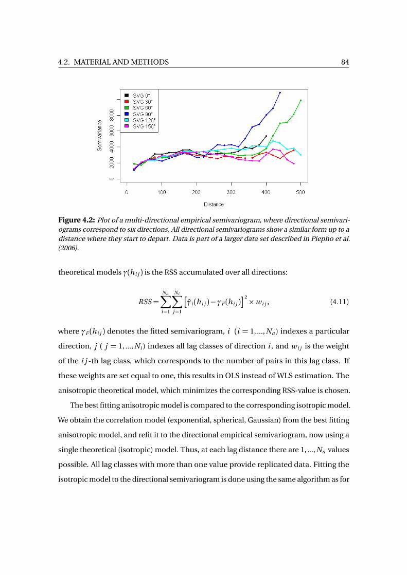
4.2. MATERIAL AND METHODS 84
Figure 4.2: Plot of a multi-directional empirical semivariogram, where directional semivari-ograms correspond to six directions. All directional semivariograms show a similar form up to adistance where they start to depart. Data is part of a larger data set described in Piepho et al.(2006).
theoretical models γ(h i j ) is the RSS accumulated over all directions:
RSS =Na∑
i=1
Ni∑
j=1
�
γi (h i j )−γF (h i j )�2×w i j , (4.11)
where γF (h i j ) denotes the fitted semivariogram, i (i = 1, ..., Na ) indexes a particular
direction, j ( j = 1, ..., Ni ) indexes all lag classes of direction i , and w i j is the weight
of the i j -th lag class, which corresponds to the number of pairs in this lag class. If
these weights are set equal to one, this results in OLS instead of WLS estimation. The
anisotropic theoretical model, which minimizes the corresponding RSS-value is chosen.
The best fitting anisotropic model is compared to the corresponding isotropic model.
We obtain the correlation model (exponential, spherical, Gaussian) from the best fitting
anisotropic model, and refit it to the directional empirical semivariogram, now using a
single theoretical (isotropic) model. Thus, at each lag distance there are 1, ..., Na values
possible. All lag classes with more than one value provide replicated data. Fitting the
isotropic model to the directional semivariogram is done using the same algorithm as for

4.2. MATERIAL AND METHODS 85
the anisotropic case. Only the respective objective functions differ slightly. Specifically,
there is no subscript for the range parameterφ. Again, we use an F -statistic to decide
whether to use the isotropic or anisotropic model:
F2 =(RSSi so −RSSa ni so)/(DFi so −DFa ni so)
RSSa ni so/DFa ni so. (4.12)
The isotropic model has three parameters, and the anisotropic model has Na − 1 ad-
ditional parameters, since there is a range parameter for each of the Na directions,
hence DFi so =NSV −3 and DFa ni so =NSV −Na n g l e −2, where NSV is the number of all
semivariances of the directional empirical semivariogram, and Na is the number of
directions/angles. Subsequently, F2 is compared to an F (Na −1;DFa ni so) distribution
and the p -value is obtained. If this p -value falls below a threshold value the anisotropic
model is chosen. In our investigation, threshold p -values of 10−5 (WLS) and 10−3 (OLS)
proved to produce reasonable results, leading to decisions that coincided with the visual
inspection. As pointed out previously, the test is approximate in that it is based on the
assumption of independence and normality of the empirical semivariogram estimates.
Figure 4.3: Plot of variances of semivariances (VSV) of 6 directional empirical semivariograms.Values correspond to the directional semivariograms of Figure 4.2. Up to a distance of 220distance units, this function is almost constant. VSV-values start to increase slightly between220 to 320 distance units and increase rapidly for distances greater than 320.

4.2. MATERIAL AND METHODS 86
An important point in using the F -statistic (4.12) is the choice of a cut-point, i.e.
a specific distance at which the empirical semivariogram is cut, and all lag classes of
distances greater than the cut-point distance are discarded. As one can see in Figure
4.2, semivariances of different directions lie close together for smaller distances up to a
point at which they start to scatter, which is a characteristic feature of isotropic models.
This particular example depicts data for which an isotropic model was chosen. If the
whole range of distances would have been used, the F -test would have been significant,
thus preferring an anisotropic model.
A useful tool in choosing this cut-off value is a plot of the variances of semivariances
(VSV), the rationale being that we do not need to fit the model beyond a point where
the sill has been reached for all directions. An example, which shows this type of plot is
depicted in Figure 4.3, where the same data is use as for Figure 4.2. At a distance of 220
distance units, VSV-values start to increase, whereas at distances smaller than 220 they
are approximately equal. At distances greater than 320 distance units the VSV-values
start to increase rapidly.
Figure 4.4: (1s t ) : Plot of variances of semivariances (VSV) for 6 directional empirical semivar-iograms. In contrast to Figure 4.3, VSV-values are not nearly constant for shorter distances. Theminimum is located at a mid-range distance. (2nd ) : Six directional empirical semivariograms,whose VSV plot is shown in the 1s t plot. Data is part of a larger data set described in Piepho et al.(2006).

4.3. THREE APPROACHES TO BG-SMOOTHING 87
For anisotropic models the multidirectional semivariogram as well as the VSV-plot
do not look similar compared to isotropic cases. An example is depicted in Figure 4.4.
In the VSV-plot (1s t plot) there is an initially increasing variance, which decreases after
a local maximum to a local minimum. In our experience this is a common feature
of anisotropic models fitted to cDNA microarray data, if one would classify them as
anisotropic by visually inspecting the directional semivariogram. In our complex proce-
dure this local minimum is chosen to trim the multidirectional semivariogram. Thus,
only distances smaller than or equal to this cut-point are used to fit the anisotropic
and isotropic models. Choosing a cut-point is restricted to distances greater than a
minimum distance to avoid having too few degrees of freedom performing the F -test.
To obtain a reasonable cut-point we first compute all local minima of the empirical
VSV-function minloc(VSV). Subsequently, all minima are removed that are located at
distances smaller or equal to a threshold distance as described. If there are local minima
left, the smallest of these minima is chosen. In case of a single minimum, this is chosen.
Otherwise, ratios
ri =vi
vi−1, i ∈ {2, ..., N } (4.13)
are computed, where vi corresponds to the i -th VSV-value larger then a minimum
threshold distance (100 distance units), and N is the largest index referencing a specific
VSV-value. We choose the distance with the largest ratio ri as cut-point.
4.3 Three Approaches to BG-Smoothing
As stated in Section 4.1, we used three different algorithms for locally smoothing the BG
values in a block-wise manner.
1. The most complex procedure comprises each step as described in Section 4.2.4
and Section 4.2.5. The obvious complexity of this algorithm is increased by the
fact that in case a specific global trend model resulted in a singular Kriging system,

4.3. THREE APPROACHES TO BG-SMOOTHING 88
where no smoothed BG values could be obtained, the second best global trend
model is chosen. If this fails the next one is used. We will refer to this complex
approach by OK.
2. This approach is a simplification of the first one. We left out the step on checking
whether there is sufficient information for fitting a spatial model and used the con-
stant global trend model. Kriging estimates were obtained using the best fitting
isotropic model among the three theoretical correlation models (Gaussian, expo-
nential, spherical). Thus, we did not have to perform any F -test since anisotropy
was not considered. We will refer to this approach by OKiso emphasizing that we
focus on isotropic models.
3. This approach consists of 2D-LOWESS on BG values. The concept of 2D LOWESS
is quite simple. For a point y at location x a LOWESS estimate y is required. Let
f be a number between 0 and 1 (span) and let q = f ×n , q is truncated to an
integer value. Among n points a neighborhood of point x consisting of points
x i , i ∈�
1, ...,q
, q ≤ n is selected. A specific weight is assigned to each point
within this neighborhood:
w i =w (x i ) =
¨
1−�
ρ(x i −x )d (x )
�3«
, (4.14)
where ρ is a distance function, d (x ) is the distance of x to the q-th nearest x i
(tri-cubic weight function). A quadratic function using weights w i is fit to values yi
in order to obtain an estimate y at location x (Cleveland et al., 1988; Cleveland &
Grosse, 1991). LOWESS estimates were obtained for BG values using a span-value
f = 0.35 with four iterations to obtain a robust fit. We will refer to this method by
Loess, which is the name of the R-function that we used.
When we applied the geostatistical framework (OK, OKiso), we used a lag distance of
20 distance units, and 25 lag classes, which resulted in a maximum lag distance of

4.4. BACKGROUND CORRECTION METHODS 89
500 distance units for computation of the empirical semivariograms. The spots of the
SVS-data were arranged in a grid with separation distance of approximately 20 distance
units in both directions, which led to this choice of parameters.
4.4 Background Correction Methods
All three BG-smoothing algorithms, as described in the previous section, were used
in conjunction with two BGC methods, one of which has been found to be superior
in a comparison study on different BGC methods (Ritchie et al., 2007). Ritchie et al.
recommend the use of normexp+offset, which extends the normexp algorithm. The
normexp algorithm is performed on BG subtracted signal intensities. The observed
intensities X are the result of a convolution of the true signal S and a noise component
Y :
X =S+Y , S ∼ exp1
α, Y ∼N (µ, σ2). (4.15)
The normal distribution for the noise component is truncated at zero, which models
non-negative signal values. A conditional expectation estimates the signal value S
(McGee & Chen, 2006). This model is fitted to each dye-channel separately. Kernel
density parameter estimation is done by using Maximum Likelihood (ML). For the
normexp+offset method a small value is added to the corrected intensities which moves
the corrected intensities away from zero and stabilizes the variance for small log-ratios
(Ritchie et al., 2007). The typical fishtail effect in M-vs-A plots for small A-values is
mitigated (see Figure 1 in Ritchie et al. 2007). Here M = log2 (R)− log2 (G ), A = 0.5×
log2 (R)+0.5× log2 (G ), R refers to signal from the red dye-channel (Cy5), and G refers to
the green channel (Cy3). In the present study we used an offset-value of 50 as suggested
by Ritchie et al. (2007). The normexp method is similar to the BG adjustment within the
RMA algorithm for Affymetrix oligonucleotide microarrays (Irizarry et al., 2003).
For comparison, we also applied the traditional BG subtraction FG-BG (subtract),

4.5. SELF-VERSUS-SELF DATA 90
and the Edwards BGC method. The latter method avoids negative BG corrected intensi-
ties by using a smoothing function of FG-BG values and a threshold δ. If S represents
the BG corrected value, Edwards (2003) defined it as:
S =
FG − BG , if FG − BG >δ
δ×exp [1− (BG +δ)/FG ] , otherwise(4.16)
We also applied the normexp and normexp+offset algorithms without BG smooth-
ing to assess the effect of BG-smoothing prior to BGC. Thus, there were ten BGC
methods overall: subtract, Edwards, Loess_normexp, OK_normexp, OKiso_normexp ,
Loess_normexp+offset, OK_normexp+offset, OKiso_normexp+
offset, normexp, and normexp+offset.
4.5 Self-versus-Self Data
To simulate differentially expressed genes and to assess the behaviour of different
BGC methods under the null-hypothesis (H0) we used a self-versus-self (SVS) dataset
consisting of six custom-made microarrays. In total 25392 spots were assigned to
48 blocks, each one consisting of 23× 23 spots (rows × columns). Each microarray
represents a replicate of an Arabidopsis mRNA pool of plants, which were grown for six
weeks in short days. Rosette leaves from 12 plants were harvested, pooled and total RNA
extracted. 100mg of RNA were labeled with Cy3- or Cy5-dCTP1 and hybridized overnight.
The microarrays contain gene-specific DNA fragments that were amplified by PCR2.
Scanning was performed with a ScanArray4000 (PerkinElmer). Scanning parameters
were set so that no more than one to four spots were saturated in each sub-grid. Spot
intensities were obtained by using Imagene image analysis software with automated
1Deoxycytidine Triphosphate linked to Fluorescence Dye Cy3 or Cy52Polymerase Chain Reaction

4.5. SELF-VERSUS-SELF DATA 91
spot finding followed by manual checking and adjustment (Hilson et al., 2004; Little et
al., 2007).
We used the SVS-data to simulate subsets of differentially expressed (DE) genes. At
first, we allocated two genotypes randomly to each channel of an individual microarray.
Then, we simulated 10% of all 25392 genes as DE. We randomly selected four subsets,
each consisting of 2.5% (634) of all genes. For one subset, half of the raw signal intensities
were multiplied with an artificial fold change (FC) in genotype one, the other half were
multiplied with the same FC in genotype two. This corresponds to up- and down-
regulation of genes for one genotype. We used FC-values of 1.5, 2, 3, and 5 to simulate
different classes of DE genes. To obtain more robust results, we repeated the complete
simulation procedure, consisting of genotype allocation and DE simulation, four times
and averaged the results. For comparing the accuracy of BGC methods, we repeated
these steps with FC-values of 2, 3, 5, and 10 to cover a wider range of DE. To adhere to
the assumption that only a small number of genes are usually expected to be DE, we
additionally created a dataset that consisted of only 5% DE genes with FC=3. Therefore,
we obtained three additional datasets from the SVS-data, with known subsets of DE
genes. These datasets were used to classify and assess all ten BGC methods.
After applying the three BG smoothing algorithms and/or BGC, the data were nor-
malized prior to estimating genotypic differences. A single chip was normalized with
Loess-within-chip-normalization (R-package limma). The log-ratios of microarrays
were then scaled to have the same absolute median deviation, which is sometimes
called between-chip-normalization (Smyth & Speed, 2003; R-package limma). Since
Loess-normalization operates on log-ratios, any spot with higher BG than signal inten-
sity represented a missing value for the traditional BG subtraction (subtract). All other
BGC methods avoid negative BG corrected values.

4.6. COMPUTING PAIR-WISE LINEAR CONTRASTS 92
4.6 Computing Pair-wise Linear Contrasts
To assess the performance of a specific BGC procedure we estimated pair-wise linear
contrasts of two genotypes using a simple linear model. We used pair-wise contrasts
instead of heterosis contrasts, because the latter requires three genotypes instead of two,
which would result in less precise estimates. The SVS-dataset consists of data where
no truly significant results (DE genes) were expected since there were no genotypic
differences. Therefore, we allocated two genotypes (A, B) randomly to the six SVS-chips
in such a way that each chip contained both genotypes, and each genotype was present
with the same number of replicates in each dye-channel. So we had six replicates of
genotype A, and six replicates of genotype B, each one present three times in the Cy3-
channel, and three times in the Cy5-channel. DE genes were simulated as described
above. For all data, we fitted the following linear model:
yi j k =αi +βj +γk + e i j k , (4.17)
where yi j k represents the spot intensity for the i -th genotype, on the j -th array, coming
from dye-channel k , k ∈ {1, 2}, while αi , βj , and γk are fixed effects for genotype, array
and dye, respectively. The term e i j k represents the i.i.d. distributed residual error with
e i j k ∼N (0,σ2). Subsequently, differential gene expression of genotypes A and B was
quantified by subjecting expression signals to an ordinary t -test using the appropriate
linear contrast based on an OLS fit of the linear model (Searle, 1971).
We also used the moderated t -statistic to identify DE genes. This is an empirical
Bayes approach, which makes use of all estimated sample variances; these are shrunk
toward a pooled estimate. Using the moderated t -statistic makes inference far more
stable, especially in small microarray experiments (Smyth, 2003). We used the same

4.7. IMPLEMENTATION 93
model as shown above. The moderated t-statistic is defined as:
t g j =βg j
s gpυg j
, (4.18)
where βg j is the j -th estimated contrast of gene g , and υg j is the j -th diagonal element
of the estimated covariance matrix for the contrast matrix of gene g , Var (βg ) =C T VgC s 2g .
Matrix C defines the contrasts to be estimated for the g -th model fit, and Vg s 2g is the
estimated covariance matrix of the coefficient estimator αg . The posterior mean of the
sample variance s 2g of gene g is defined as:
s 2g =
d 0s 20 +d g s 2
g
d 0+d g, (4.19)
where s 2g is the residual variance estimator for gene g , with d g residual degrees of
freedom. Prior information is assumed on the residuals variances for each gene by using
a prior estimator s 20 with d 0 degrees of freedom, which are estimated from the data. The
relation between the residual variance of gene g and these prior values is expressed by:
1
σ2g
∼1
d 0s 20
χ2d 0
. (4.20)
See Smyth (2003) for a thorough development of this empirical Bayes methodology.
We adjusted p -values for multiplicity by using Storey’s q-value (Storey, 2002). This
type of adjustment was developed for very large numbers of comparisons and is there-
fore a natural choice for microarray data comprising of 25392 genes.
4.7 Implementation
All of the previously described steps were implemented using the freely available statis-
tical language R (http://cran.R-project.org). Variogram calculations, non-linear

4.8. RESULTS 94
OLS/WLS fitting of theoretical models to isotropic semivariograms, and ordinary Krig-
ing were performed using the geoR package (Ribeiro Jr. & Diggle, 2001). Non-linear
OLS/WLS estimation of isotropic/anisotropic models for multidirectional semivari-
ograms was done with the optim function of the R stats package. Specifically, we
used the “L-BGFS-B” algorithm, which allows box-constraints (Byrd et al., 1995) to set
lower and upper bounds. BGC, normalization and identifying differentially expressed
genes using the moderated t -statistic were performed using the limma package. Loess-
smoothing was done using the R-function loess. Fitting the linear model was done
with the lm function, pair-wise linear contrasts were computed with the glht function
of the multcomp package. FDR-adjustment was done with the qvalue package.
4.8 Results
Table 4.1 outlines the results obtained for all ten BGC approaches for the SVS-data with
four classes of simulated DE genes, at simulated Fold Changes (FC) of 1.5, 2, 3, and 5,
using (4.17) with ordinary t -tests of pair-wise linear contrasts, averaged over four simula-
tion cycles. Raw p -values were adjusted for multiplicity by Storey’s (2002) q-value, which
Table 4.1: Number of truly significant discoveries for ten different BGC methods using ordinaryt-tests. Columns correspond to specific simulated Fold Changes at different significance levels(α= 5%, α= 10%). Results were averaged over four independent simulation cycles, and adjustedfor multiplicity using Storey’s q-value
α= 5% α= 10%FC=1.5 FC=2 FC=3 FC=5 FC=1.5 FC=2 FC=3 FC=5
subtract 27.75 35.50 33.50 37.25 43.25 51.75 47.75 54.00
Edwards 85.25 222.75 378.00 506.00 169.50 349.50 501.00 584.00normexp 19.50 49.25 99.75 153.25 115.75 256.75 442.00 567.50
normexp+offset 34.50 93.75 187.25 297.75 130.50 290.50 478.75 590.75
OK_normexp 18.75 46.25 92.00 135.00 106.75 241.75 414.25 547.75
OKiso_normexp 69.25 202.50 387.75 536.75 158.00 341.50 527.25 616.75
Loess_normexp 86.25 226.75 428.50 572.25 176.25 372.75 547.25 619.50
OK_normexp+offset 33.00 79.00 167.00 252.75 124.00 281.00 457.50 584.25
OKiso_normexp+offset 85.75 225.50 431.25 569.25 171.00 366.50 544.50 622.00
Loess_normexp+offset 100.00 259.50 465.00 590.75 189.75 397.00 560.75 624.25
simulated DE genes 634 634 634 634 634 634 634 634

4.8. RESULTS 95
resulted in observed false positive rates ranging from 4.78% (Loess_normexp+offset)
to 6.04% (normexp) at the 5% significance level and 9.08% (normexp, OK_normexp) to
9.84% (Edwards) at the 10% nominal α-level. The subtract method performed worst.
It detected by far the fewest simulated DE genes and had by far the highest observed
false positive rate. The best performing method is Loess_normexp+offset. For each
class corresponding to a specific simulated FC, this method identified most DE genes.
Smoothing BG values prior to BGC clearly increased power (Figure 4.6, 1s t plot), and
lowered the proportion of false discoveries (Figure 4.5, 1s t plot).
Table 4.2: Number of truly significant discoveries for ten different BGC methods using moder-ated t-tests. Columns correspond to specific simulated Fold Changes at different significancelevels (α= 5%, α= 10%). Results were averaged over four independent simulation cycles, andadjusted for multiplicity using Storey’s q-value.
α= 5% α= 10%FC=1.5 FC=2 FC=3 FC=5 FC=1.5 FC=2 FC=3 FC=5
subtract 49.25 45.25 57.50 60.00 58.50 54.25 68.00 68.25
Edwards 122.50 400.25 558.00 613.00 223.75 492.00 596.75 625.25normexp 231.75 500.00 620.50 633.50 321.00 566.00 629.00 633.50
normexp+offset 230.50 488.75 617.50 633.75 317.25 558.00 628.75 633.75
OK_normexp 221.75 506.00 622.75 632.75 309.50 566.00 631.00 633.25
OKiso_normexp 244.25 550.50 628.00 633.75 330.75 585.75 631.50 633.75
Loess_normexp 228.00 542.50 624.25 633.75 334.75 586.00 629.25 634.00
OK_normexp+offset 226.00 495.00 620.25 632.50 309.75 559.50 630.50 633.25
OKiso_normexp+offset 260.75 557.00 628.50 634.00 346.75 590.50 632.00 634.00
Loess_normexp+offset 270.75 566.75 628.00 633.75 369.00 596.25 630.50 634.00
simulated DE genes 634 634 634 634 634 634 634 634
A similar outcome was observed when Smyth’s moderated t -statistic was used to
identify DE genes (Table 4.2). The observed false positive rates were smaller than for the
ordinary t -statistic (OK_normexp 2.72% to 4.2% for Edwards at the 5% significance level;
OK_normexp 6.74% to 8.72% for Loess_normexp at the 10% significance level). The sub-
tract method had by far the highest observed false positive rates (88.39%, 88.59%), as for
the ordinary t -statistic. An obvious feature of the moderated t -statistic is the increased
number of identified DE genes compared to using ordinary t -tests. This is the result of
borrowing information across genes, and therefore, having more degrees of freedom
available. Application of OKiso and Loess prior to normexp and normexp+offset BGC

4.8. RESULTS 96
methods increased the power (Figure 4.6, 2nd plot) and decreased the number of false
discoveries (Figure 4.5, 2nd plot). This is independent of the method used to detect DE
genes, since ordinary t -tests (Table 4.1), as well as moderated t -tests (Table 4.2) both
benefit from smoothing BG-values prior to BGC.
Table 4.3: Number of true discoveries for ten different background correction methods usingordinary t -tests and moderated t -tests. Columns correspond to different significance levels at asingle simulated Fold Change. Results were averaged over four independent simulations, andadjusted for multiplicity using Storey’s q-value approach.
Fold Change 3ordinary-t moderated-t
α= 1% α= 5% α= 10% α= 0.1% α= 1% α= 5%
subtract 0 43.50 61.50 0 40.50 74.25
Edwards 5.25 627.50 881.25 0 618.25 1067.50normexp 0 41.00 344.50 343.75 1070.50 1232.25
normexp+offset 0.25 59.75 604.00 329.25 1047.25 1227.25
OK_normexp 0 26.00 243.25 266.25 1082.25 1235.50
OKiso_normexp 0 452.50 878.50 788.00 1185.75 1251.25
Loess_normexp 4.00 636.25 966.25 611.50 1163.25 1246.50
OK_normexp+offset 0 50.25 488.50 287.50 1059.50 1229.50
OKiso_normexp+offset 21.25 632.75 953.50 916.25 1204.75 1253.00
Loess_normexp+offset 24.75 765.25 1023.25 968.50 1218.00 1258.25
simulated DE genes 1269 1269 1269 1269 1269 1269
To circumvent misleading inference due to a too large proportion of DE genes,
we also applied all ten methods to the SVS-data with a single class of DE-genes. We
simulated 5% DE genes with FC=3 as described above and independently repeated the
simulation four times. Results of the ordinary t -tests as well as those of the moderated
t -tests are shown in Table 4.3. These results confirm our findings for the SVS-data
with four classes of 10% simulated DE genes. The complex and time-consuming OK
approach (OK_normexp, OK_normexp+offset) does not perform as good as the other
two BG-smoothing algorithms (OKiso, Loess). We conclude that applying this complex
framework as described in Section 4.2 is not justified. We do not include the results of
this BG smoothing algorithm in Figure 4.5 and Figure 4.6. As one can see in Tables 4.1,
4.2 and 4.3, performing the traditional BG subtraction is the worst BGC method overall.
To further assess the different BGC approaches we investigated the trade-off between

4.8. RESULTS 97
Figure 4.5: Trade-off between the number of selected genes and the number of false discoveriesfor the SVS-data with four classes of DE genes. Results were averaged over four independentsimulations, and adjusted for multiplicity using Storey’s q-value approach. (1s t ) : DE geneswere identified using ordinary t -tests. (2nd ) : DE genes were identified using moderated t -tests
the number of genes that were termed significant and the number of false discoveries
among them. These findings are depicted in Figure 4.5. The subtract method is not
shown, because the very large numbers of false discoveries would distort this plot.
The corresponding line would run way left of the others. Extending established BGC
methods (normexp, normexp+offset) by BG smoothing (Loess, OKiso) lowered the
proportion of false discoveries (Figure 4.5) and increased the power of finding DE genes
(Figure 4.6).
The raw SVS-data served as means to check whether different BG smoothing meth-
ods perform as expected under the null-hypothesis (H0), respectively, if the proportion
of false significant results exceeds the expected empirical error rate (size). In case of no
significant differences between both simulated genotypes one would expect that the
observed p -values are uniformly distributed, p ∼U (0, 1). This corresponds to a straight
line in the plot of nominal significance levels vs. empirical error rates as shown in Figure
4.7. None of the six methods exhibit peculiar departure from the expected proportion
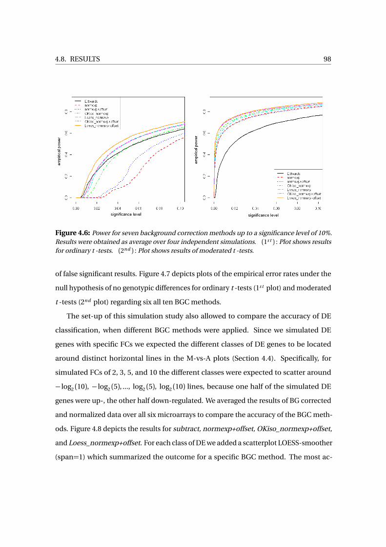
4.8. RESULTS 98
Figure 4.6: Power for seven background correction methods up to a significance level of 10%.Results were obtained as average over four independent simulations. (1s t ) : Plot shows resultsfor ordinary t -tests. (2nd ) : Plot shows results of moderated t -tests.
of false significant results. Figure 4.7 depicts plots of the empirical error rates under the
null hypothesis of no genotypic differences for ordinary t -tests (1s t plot) and moderated
t -tests (2nd plot) regarding six all ten BGC methods.
The set-up of this simulation study also allowed to compare the accuracy of DE
classification, when different BGC methods were applied. Since we simulated DE
genes with specific FCs we expected the different classes of DE genes to be located
around distinct horizontal lines in the M-vs-A plots (Section 4.4). Specifically, for
simulated FCs of 2, 3, 5, and 10 the different classes were expected to scatter around
− log2 (10), − log2 (5), ..., log2 (5), log2 (10) lines, because one half of the simulated DE
genes were up-, the other half down-regulated. We averaged the results of BG corrected
and normalized data over all six microarrays to compare the accuracy of the BGC meth-
ods. Figure 4.8 depicts the results for subtract, normexp+offset, OKiso_normexp+offset,
and Loess_normexp+offset. For each class of DE we added a scatterplot LOESS-smoother
(span=1) which summarized the outcome for a specific BGC method. The most ac-

4.8. RESULTS 99
Figure 4.7: Empirical error rates under the null hypothesis, i.e. there were no DE genessimulated, thus, there no differences among the simulated genotypes. (1s t ) : Plot showsresults of ordinary t -tests. (2nd ) : Plot shows results of moderated t -tests.
curate method is Loess_normexp+offset. The lines of the LOESS-smoother for this
method reflect the expectation (dotted lines) to the greatest extend and showed the
lowest degree of curvature over the range of expression intensities (X-axis).
Results obtained without using the offset were similar but less accurate, i.e. the
LOWESS-smoothers were farther away from the expectation (not shown). The OK-
iso_normexp method performed better in comparison to Loess_normexp, which in
turn outperformed normexp. Using BG smoothing prior to BGC resulted in more stable
patterns of DE, i.e. the simulated DE genes were less dependent of the mean expression
level and the Fold Changes better reflected the imputed simulated Fold Changes (dotted
lines). The upper left plot of Figure 4.8 (subtract) reveals the most severe departure from
the expectation (dotted lines).

4.8. RESULTS 100
Figure 4.8: Exemplary M vs. A plot averaged over all microarrays of the self-vs-self data for onesimulation cycle. Classes of simulated DE genes are colored (red: FC=2, blue: FC=3, orange:FC=5, green: FC=10). Dotted gray lines correspond to the expected value of each DE-class(log2-scale), solid colored lines correspond to lines of the LOWESS-smoother with span=1 perDE-class. The M-vs-A plot for the subtract BGC method (1s t plot) show the typical “fishtail”effect, i.e. the lower the mean intensity the higher is the variance of log-ratios.

Chapter 5
General Discussion
5.1 The Monte Carlo Approach
The MC approach to the residual analysis of LMs has several applications. First and most
importantly, it facilitates the interpretation of informal procedures for model checking,
e.g. various residual plots. We introduced three examples of diagnostic plots, whose
practical use was improved by adding simultaneous tolerance bounds. These bounds
reflect the null distribution of a particular set of residuals, and can be computed from
simulation. There are always non-zero correlations between pairs of residuals, because
n residuals carry only (n −p ) degrees of freedom (Draper & Smith, 1998, p. 206). This
correlation structure has to be accounted for, since the larger p gets the more severe
becomes its influence. Tables 2.1 and 2.2 as well as Figures 2.3 and 2.4 make this obvious.
The correlation structure can easily be integrated in the simulations by applying (2.7).
For LMs, studentized residuals are pivotal statistics (Cox & Hinkley, 1974). This enables
computing simultaneous tolerance bounds such that the coverage of the resulting STBs
or STIs becomes exact for N →∞. We suggest to use studentized residuals throughout,
which corresponds to standardizing the set of residuals to have an expected value equal
to zero and variance equal to one. Studentization has the great benefit of additionally
101

5.1. THE MONTE CARLO APPROACH 102
accounting for the estimation variance of each individual residual, which can differ
substantially.
We exemplified the MC approach for diagnostic plots by using QQ-plots with STB for
normality and a plot of residuals vs. predicted values with STI for homoscedasticity and
outlier detection. The latter can also be checked employing a plot of absolute values or
squares of residuals vs. predicted values, where an STB for the corresponding regression
line can be added (3r d plots of Figures 2.5 - 2.8). This plot is particularly useful to assess
whether the residual variance depends on predicted values. It may give a hint that an
appropriate data transformation is required, which can remedy this problem in many
cases. This type of plot is also sensitive for outlying observations, even in situations,
where the slope of the corresponding regression line is not extreme compared to its null
distribution. Large absolute (or squared) residuals shift the remaining residuals toward
zero, which results in a regression line violating the lower bound of the corresponding
STB. This is obvious in the plot of the regression log (M )∼ log (S) for the mussels data in
Section 2.5, where observation 48 was removed (Figure 2.7, 3r d plot). The associated
MC-test for the regression slope (Section 2.5.2) was not significant (p -value=0.61),
which can be taken as indication that informal procedures (diagnostic plots) are more
useful than formal testing.
Although an STB inherently defines a valid level-α test, we suggest to use it mainly
as a tool in deciding about the assumed normality and not as formal test. Basically, STBs
are a straight forward development of the envelopes for half-normal plots, as suggested
by Atkinson (1981, 1985), where now simultaneous coverage of the point-wise toler-
ance intervals is considered. Furthermore, we suggest way more MC simulations than
Atkinson did (N=19) to obtain a better picture of the correct null distribution. Today,
more than 20 years after the proposal of envelopes, modern computers are capable of
computing several thousands of simulation cycles in a short time. By simulating at least
N=5000 samples, one obtains a high resolution picture of the null distribution, i.e. the

5.1. THE MONTE CARLO APPROACH 103
bounds of the corresponding STB are very smooth.
Frequently, plots of the residuals vs. predicted values are used to assess LMs regard-
ing homoscedasticity and the presence of outliers. These plots benefit from adding
an STI, which covers (1−α)100% of all N simulated residual vectors completely. The
bounds of the STI can be computed with the quantile-based bisection algorithm (2.4.1),
which terminates very fast, because for each simulated vector only the smallest and the
largest residuals are required. This fast convergence makes it feasible to compute STIs
for different values of the α-level. Sometimes, a single suspiciously deviant residual is
not necessarily outlying, which can be checked by employing different tolerance levels.
Moreover, one should always combine the information from different diagnostic plots.
A residual is more likely to be truly outlying in case it appears outside the simultaneous
tolerance bounds in different diagnostic plots. For example, in Section 3.6.1, where
we apply the simulation approach to an LMM, the 4t h observation of subject 29 (29.4)
appears outside the 95.00% STI in the plot of studentized conditional residuals (CR)
vs. predicted values (3r d plot of Figure 3.4). It is, however, neither located outside the
99.00% STI, shown in the same plot, nor is it located outside the 95.00% STB in the
corresponding QQ-plot (3r d plot of Figure 3.3). Thus, when combining the information
of both plots, observation 29.4 cannot be considered as truly outlying. This equally
applies to the residual analysis of LMs and LMMs.
The same plots as used for the residual analysis of LMs can be used to assess LMM
residuals. The main difference is that there is more than one set of residuals for LMMs
and that studentized residuals are not pivotal. Hilden-Minton (1995) showed that CRs e
are confounded with random effects b and that EBLUPs Z b are confounded with errors
e . Hilden-Minton (1995) and Nobre and Singer (2007) proposed a linear transformation
of CRs, which transforms CRs into a lower-dimensional space of uncorrelated residuals,
which is identical to the residual space of the corresponding fixed effect analysis, i.e.
where all random effects are taken as fixed. We see two distinct problems with any

5.1. THE MONTE CARLO APPROACH 104
orthogonal transformation of residuals, either in the LM or LMM context. Firstly, one
cannot identify any outlying observations, because each transformed value is a linear
combination of the untransformed quantities, which was also stressed by Cook and
Weisberg (1982). Secondly, we expect orthogonal transformations to amplify the super-
normality effect, which is the phenomenon that non-normal quantities appear more
normal, when they are estimated. To our knowledge, the term supernormality goes back
to Atkinson (1985). The simulation study of Section 2.4.4, where we used various non-
normal distributions and different LMs, may serve as indication that supernormality
is really amplified by orthogonalization. We used two different linear transformations
and applied the Shapiro-Wilk (SW) test to the set of transformed values. The empirical
power for both (Table 2.2, SWLUS and SWcBLUS) were consistently way below the one for
the raw, untransformed residuals (SW without subscript), which was also tested with the
SW-test. The MC-version of the SW-test (SWMC) yielded the best power overall, and it
was up to 33% better than its non-MC counterpart (log-normal alternative distribution
for design 7). We see no reason why this feature should not carry over from LM residuals
to LMM residuals, since in both cases there are fewer transformed (orthogonalized)
than untransformed values, and the linear transformation can be seen as application of
the central limit theorem.
As stated above, studentized residuals for LMMs are not pivotal quantities. Therefore,
one cannot assume validity of the simulated null distributions a-priori. We tackled this
problem by carrying out a simulation study, to assess nominal error rates associated
with the simultaneous tolerance bounds of different types of studentized residuals
(CRs, random effects). We obtained results for balanced (Table 3.1) and for unbalanced
designs (Table 3.2), both with varying complexity, where we additionally simulated three
different ratios of variance components γ, γ ∈ {0.1, 1, 10}. These results do not raise
concerns about not meeting an empirical error rate (size) of 5%, when we used α= 0.05
for computation of the simultaneous tolerance bounds from simulated data. Admittedly,

5.1. THE MONTE CARLO APPROACH 105
these conclusion only apply to the LMMs, which were used in this simulations study,
and one would have to test each individual LMM separately. This is, of course, not
feasible, but at this point of time there is no indication that the results of this simulation
study should not carry over to other LMMs.
Furthermore, we have shown the usefulness of the simulation approach for the
residual analysis of LMMs by applying it to three datasets, which were used in other
publications (Sections 3.6.1 - 3.6.3). By applying (3.8), it is obvious that the simulation
approach for LMMs is in fact a parametric bootstrap approach (Efron & Tibshirani,
1993), where each random component of the model is simulated by drawing a sample
from a specific normal distribution with covariances equal to their estimates. Results
presented in this thesis support the conclusion that using studentized residuals is always
better than simple standardization of residuals. This is particularly obvious from looking
at Figure 3.10, where we plotted standardized (5t h plot) and studentized random effects
(6t h plot) with their associated STBs for the LMM fitted to the Orthodont data (Section
3.6.3).
Besides using simulation for the residual analysis of LMs or LMMs based on diagnos-
tic plots, one can use this approach for assessing model assumption either by employing
formal significance tests, e.g. the Shapiro-Wilk test for normality (Thode, 2002) and
the Levene-test for homoscedasticity (Levene, 1960; Piepho, 1996a), or by constructing
MC-tests tailored for specific model assumptions. We proposed a diagnostic plot of
absolute values or squares of studentized residuals vs. predicted values and to obtain
the corresponding regression line. The null hypothesis that this slope is equal to zero
can be tested with an F -test (Draper & Smith, 1998). This idea can be transferred to
the simulation approach, where the observed slope is compared to the slopes of the
regression lines coming from simulated H0 data (see Section 2.5.2). There are many
other tests of normality, homoscedasticity or linearity that can be constructed from
simulated data. Our results and those by other authors (e.g. Dufour et al., 1998) showed

5.1. THE MONTE CARLO APPROACH 106
that MC-versions are more powerful and/or achieve better size control than the naive
application to residuals of tests proposed for observed data.
In Section 2.4.4 we presented a simulation study, where several tests for normality
(Thode, 2002) were applied as MC-tests and once applied to the observed, studentized
residuals of seven LMs with varying numbers of observations n and parameters p .
For six different alternative, non-normal distributions, the MC approach was superior
throughout, with only very few exceptions. For example, the Shapiro-Francia (SF) test
had 65% higher power when applied as MC-test compared to its non-MC version (Table
2.2, log-normal alternative distribution for design 7). This simulation study also revealed
that orthogonalization of the residuals is not a real alternative to simulating their null
distribution. Of course, orthogonalization also accounts for the correlation structure
of the residuals by simply removing it, but it transforms the set of n residuals to a
(n −p )-dimensional space by forming linear combinations of the original quantities at
the same time. We conclude that supernormality occurs, and that the loss of degrees
of freedom both negatively affect the test results and, therefore, explain why MC-tests
outperform their non-MC counterparts, which are applied to orthogonal residuals.
When applying MC hypothesis tests, the number of simulations is not required to
be as large as for diagnostic plots. For example, Dufour et al. (1998) use only N = 99
MC simulations, and report that increasing this number results only in small gains in
power. One can reduce the number of simulations even more by employing sequential
MC-tests, as proposed by Besag and Clifford (1991). The rationale of this concept is that
if there is not enough evidence against H0 in the first l simulation cycles, it is unlikely
that H0 will be rejected for the full set of MC simulations. The number of simulations is
not fixed, instead a constant h is chosen which depends on the significance level α. Let
Tob s be the test statistic obtained for the observed data, and let T MC be the test statistic
for simulated data under H0. In case h times T MC ≥ Tob s after the l -th simulation, the
procedure stops, and a MC p -value can be computed as p MC = h/l . In case the full

5.2. SMOOTHING BACKGROUND INTENSITIES 107
number of simulations (N ) were performed, where g times T MC ≥ Tob s and g < h, the
corresponding p -value can be calculated as p MC = (g + 1)/(N + 1) (Besag & Clifford,
1991). Therefore, if one is only interested in a MC p -value, our method can be improved
in terms of computational time. Silva et al. (2009) showed that the power of sequential
MC-tests is the same as for the MC-test with the full set of N simulations. The expression
α≥ h/N allows to compute the constant h according to the full set of N simulations.
Note that the precision of the sequential p -value decreases with decreasing number of
simulations. However, this might be of less importance since the smaller such a p -value
gets the more precisely it is estimated in terms of the standard error.
For omics data, the simulation approach for the residual analysis of LMs or LMMs
is directly applicable. In case of gene expression data with several thousands of genes,
where each gene is analyzed separately, using diagnostic plots is not feasible. The
sequential MC-tests could be an alternative to using diagnostic plots. Although formal
testing for model checking is generally not recommended, employing simulation based
tests for assessing model assumptions is always the better choice compared to applying
formal significance tests only once in a non-MC fashion. It could be useful to have
p -values available, providing evidence against either normality or homoscedasticity.
In case both assumptions are violated, indicated by small p -values, the corresponding
results cannot be considered reliable (Bradley, 1980, 1984). In large, explorative gene
expression studies, where possibly many results are termed significant, one could
concentrate on those significant results, with no or only little evidence of simultaneous
violation of normality and homoscedasticity. Otherwise, estimates and conclusion
based on these estimates are doubtful.
5.2 Smoothing Background Intensities
Before LMs or LMMs can be fitted to gene expression data, one has to perform complex
preprocessing of the raw data. This usually begins with BG correction (BGC), which aims

5.2. SMOOTHING BACKGROUND INTENSITIES 108
at removing the biasing contribution to the fluorescence signals introduced by non-
specifically bound cDNA molecules. In Chapter 4 we pursued the questions, whether
BGC algorithms that avoid negative expression signals (e.g. Edwards, 2003; Ritchie et al.,
2007) can be improved. Any BGC method relies on the implicit assumption of locally
constant BG values (Kooperberg et al., 2002), which is frequently not met, i.e. there is
much variation among a particular BG value of one spot and its four physical neighbors.
Therefore, we wanted to check whether smoothed BG values have positive effects on
the analysis of gene expression data or not. It is obvious from Figure 4.1 that there is
some spatial structure among the BG values, which is independent of local differences.
This implies the use of spatial smoothing methods that can make use of this correlation
structure. Figure 4.1 also reveals that BG values are sometimes more similar in one
direction than in the orthogonal direction. Geostatistical models, which make use of
directional information are called anisotropic models, and the question arose whether
directional information has to be accounted for.
To investigate both issues (1. is BG smoothing beneficial, 2. does directional infor-
mation have an effect), we implemented a complex BG smoothing algorithm (OK ),
capable of differentiating between isotropic and anisotropic models, and two simpler
BG smoothing approaches, which do not incorporate directional information (Loe s s ,
OK i so). We combined these three methods with two BGC algorithms (nor m e x p ,
nor m e x p +o f f s e t ), which both avoid negative gene expression signals and which
were found to be superior among different BGC algorithms (Ritchie et al., 2007). OK
and OK i so both rely on Kriging, which fits into the LMM framework (Robinson, 1991).
Our results are based on a self-vs-self (SVS) dataset, where biologically identical
plant material (Arabidopsis) was used to generate a gene expression dataset. Since there
were no differences in gene expression, we could artificially introduce differentially
expressed (DE) genes, thus, knowing the exact number and the corresponding Fold
Change of the DE genes. This allowed to compare the power, the accuracy, and the

5.2. SMOOTHING BACKGROUND INTENSITIES 109
number of false significant findings for each combination of BG smoothing algorithm
and BGC algorithm. We decided to use DE instead of the more complex heterosis
contrasts, because of the limited size of the SVS-dataset. Thus, only two instead of three
genotypes had to be randomly allocated to the six microarrays of the SVS-dataset, which,
due to the higher number of replicates, yielded more precise genotypic estimates. We
employed a classical approach to detecting DE genes, based on LMs (ordinary t -tests),
and an empirical Bayes approach (moderated t -tests), which remedies the problem of
usually having only few degrees of freedom available for detecting DE in microarray
experiments (Smyth, 2003).
We would propose 2D-LOWESS (Loe s s ) as BG smoothing algorithm. Loe s s and
OK i so, combined with either BGC algorithm, were both better than leaving BG smooth-
ing out in all particular points. In combination with the nor m e x p +o f f s e t BGC
algorithm Loe s s was the most accurate method (Figure 4.8), the method with the least
false significant results (Figure 4.5), and the method which had the best empirical power
(Figure 4.6). The OK i so approach was similarly successful, and we believe that the
reason why it came 2nd was that every now and then a singular Kriging system oc-
curred. This resulted in blocks of a particular microarray, which remained unsmoothed,
whereas the 2D-LOWESS algorithm smoothed each specific block of a microarray. Using
the complex algorithm (OK ) is not justified by our findings (compare Tables 4.1 - 4.3),
although there is certainly much space for improvement of each step of the pipeline as
described in Section 4.2.5.
One might argue that restricting smoothing of BG values to only some regions of
the microarray, thus treating blocks of a microarray differently, introduces further bias.
We believe, however, that confinement to blocks is, in fact, a particular strength of our
methodology because the spatial correlation structure of BG values is often restricted to
specific parts of the chip surface. This can be seen for example in the two heatmaps in
Figure 4.1. Application of smoothing methods in a block-wise manner allows accounting

5.3. CONCLUDING REMARKS 110
for these local features.
Using maximum likelihood (ML) or restricted maximum likelihood (REML) estima-
tion would be a natural approach of finding the theoretical model of spatial correlation
to be used for the OK or OKiso methods, i.e. an LMM with spatial covariance (corre-
lation) structure had to be employed. We did not use ML/REML, however, because of
the high rate of models which did not converge. Furthermore, ML/REML estimation is
way more time consuming than weighted least squares (WLS). Application of LMMs
with spatial covariance structure would also allow to smooth BG values in the same way
as Kriging does it (see Section 4.2.3), which is not surprising, since Kriging is a special
LMM (Robinson, 1991). We used Kriging instead of the LMM formulation because of
the substantial savings in computational time.
5.3 Concluding Remarks
The thesis in hand has its application in the analysis of omics data, which were and are
generated in large amounts for heterosis research. The statistical methodology used for
analyzing these data is, of course, not limited to this field of research, which makes the
results of this thesis also applicable in any other application of LMs, LMMs or two-color
cDNA microarrays.
The MC-approach for the residual analysis of LMs and LMMs has the potential to
become a standard tool for assessing different model assumptions, specifically, when
considering the development of modern computers. MC-techniques are tailored for
parallel computing, which would reduce the computational time proportionally to
the number of processing nodes, e.g. employed in multicore processors, in computer
clusters1 or in computer grids2. The conceptual and computational simplicity of this
approach allows implementing it in the statistical package of choice without much
1group of linked, tightly coupled computers2group of loosely coupled computers working together

5.3. CONCLUDING REMARKS 111
effort. The MC approach was inspired by the need to assess model assumptions for
many variables of a large metabolomics dataset, where outliers had to be identified
and normality and homoscedasticity had to be checked. Its usefulness has already
been recognized when processing the dataset of Römisch-Margl et al. (2010). This
concept was now formalized and described in a way, which is hopefully helpful for other
researchers to make use of it.
It was also shown that smoothing background intensities prior to background cor-
rection is generally beneficial. This additional step can be easily integrated into the
preprocessing pipeline for microarray data. One simply has to use an implementation
of the LOWESS algorithm (Cleveland et al., 1988; Cleveland & Grosse, 1991), which was
the best smoothing method overall. Usually high performance implementations are
available for any statistical package, e.g. function loess in the freely available statistical
package R (www.r-project.org) or PROC LOESS in the SAS system (SAS Documenta-
tion, SAS Version 9.2, 2009). It is hoped that other researchers are attracted to this
preprocessing step and that more results about its performance will be generated.
References
Arteaga-Salas, J. M., Harrison, A. P. & Upton, G. J. G. (2008). Reducing spatial flaws inoligonucleotide arrays by using neighborhood information. Statistical Applica-tions in Genetics and Molecular Biology, 7, Article 29.
Atkinson, A. C. (1981). Two graphical displays for outlying and influential observationsin regression. Biometrika, 68, 13–20.
Atkinson, A. C. (1985). Plots, transformations and regression. Oxford: Oxford UniversityPress.
Atkinson, A. C. & Riani, M. (2000). Robust diagnostic regression analysis. New York:Springer.
Becker, H. (1993). Pflanzenzüchtung. Stuttgart: Ulmer.
Beló, A., Beatty, M., Hondred, D., Fengler, K., Li, B. & Rafalski, A. (2010). Allelic genomestructural variations in maize detected by array comparative genome hybridiza-tion. Theoretical and Applied Genetics, 120, 355–367.
Besag, J. & Clifford, P. (1991). Sequential monte carlo p-values. Biometrika, 78, 301–304.
Bradley, J. V. (1980). Nonrobustness in Z, t, and F tests at large sample sizes. Bulletin ofthe Psychonomic Society, 16, 333–336.
Bradley, J. V. (1984). The complexity of nonrobustness effects. Bulletin of the Psycho-nomic Society, 22, 250–253.
Byrd, R. H., Lu, P., Nocedal, J. & Zhu, C. (1995). A limited memory algorithm for boundconstrained optimization. SIAM J. Scientific Computing, 16, 1199–1208.
Christensen, R., Pearson, L. M. & Johnson, W. (1992). Case-deletion diagnostics formixed models. Technometrics, 34, 38–45.
Cleveland, W. S., Devlin, S. J. & Grosse, E. (1988). Regression by local fitting - methods,properties, and computational algorithms. Journal of Econometrics, 37, 87–114.
Cleveland, W. S. & Grosse, E. (1991). Computational methods for local regression.Statistics and Computing, 1, 47–62.
Colantuoni, C., Henry, G., Zeger, S. & Pevsner, J. (2002). Local mean normalization of
112

References 113
microarray element signal intensities across an array surface: Quality control andcorrection of spatially systematic artifacts. BioTechniques, 32, 1316–1320.
Cook, R. D. & Weisberg, S. (1982). Residuals and influence in regression. London:Chapman and Hall.
Cook, R. D. & Weisberg, S. (1994). An introduction to regression graphics. New York:Wiley.
Cox, D. R. & Hinkley, D. V. (1974). Theoretical statistics. London: Chapman and Hall.
Cressie, N. A. C. (1993). Statistics for spatial data. New York: Wiley.
Cressie, N. A. C. & Hawkins, D. M. (1980). Robust estimation of the variogram: I.Mathematical Geology, 12, 115–125.
Deutler, T. (1991). Grubbs-type estimators for reproducibility variances in an interlabo-ratory test study. J. Qual. Technol., 23, 324–333.
Diggle, P. J. & Ribeiro Jr., P. J. (2007). Model-based geostatistics. New York: Springer.
Draper, N. R. & Smith, H. (1998). Applied regression analysis. New York: Wiley.
Dufour, J. M., Farhat, A., Gardiol, L. & Khalaf, L. (1998). Simulation-based finite samplenormality tests in linear regression. Econometrics Journal, 1, 154–173.
Edwards, D. (2003). Non-linear normalization and background correction in one-channel cDNA microarrays. Bioinformatics, 19, 825–833.
Edwards, D. & Berry, J. J. (1987). The efficiency of simulation-based multiple compar-isons. Biometrics, 43, 913–928.
Eeuwijk, F. A. van. (1995). Linear and bilinear models for the analysis of multi-environment trials: I. An inventory of models. Euphytica, 84, 1-7.
Efron, B. & Tibshirani, R. J. (1993). An introduction to the bootstrap. London: Chapmanand Hall.
Frisch, M., Thiemann, A., Fu, J., Schrag, T. A., Scholten, S. & Melchinger, A. E. (2010).Transcriptome-based distance measures for grouping of germplasm and pre-diction of hybrid performance in maize. Theoretical and Applied Genetics, 120,441–450.
Fujita, A., Sato, J. R., Oliveira Rodrigues, L. de, Ferreira, C. E. & Sogayar, M. C. (2006). Eval-uating different methods of microarray data normalization. BMC Bioinformatics,7, Article 469.
Gumedze, F. N., Welham, S. J., Gogel, B. J. & Thompson, R. (2010). A variance shiftmodel for detection of outliers in the linear mixed model. Computational Statisticsand Data Analysis, 54, 2128–2144.

References 114
Haldermans, P., Shkedy, Z., Van Sanden, S., Burzykowski, T. & Aerts, M. (2007). Using lin-ear mixed models for normalization of cDNA microarrays. Statistical Applicationsin Genetics and Molecular Biology, 6, Article 19.
Haslett, J. & Dillane, D. (2004). Application of "delete=replace" to deletion diagnosticsfor variance component estimation in the linear mixed model. Journal of the RoyalStatistical Society Series, 66, 131–143.
Höcker, N., Keller, B., Chollet, D., Descombes, P., Piepho, H. P. & Hochholdinger, F. (2008).Comparison of maize (Zea mays) hybrid and parental inbred line primary roottranscriptomes suggests organ specific patterns of non-additive gene expressionand conserved expression trends between different hybrids in a subset of genes.Genetics, 179, 1275–1283.
Henderson, C. R. (1950). Estimation of genetic parameters. Ann. Math. Sci., 21, 309–310.
Hilden-Minton, J. A. (1995). Multilevel diagnostics for mixed and hierarchical linearmodels. Dissertation, University of California, Los Angeles.
Hilson, P., Allemeersch, J., Altmann, T., Aubourg, S., Avon, A., Beynon, J. et al. (2004). Ver-satile gene specific sequence tags for Arabidopsis functional genomics: Transcriptprofiling and reverse genetics applications. Genome Research, 14, 2176–2189.
Huber, W., Heydebreck, A. von, Sültmann, H., Poustka, A. & Vingron, M. (2002). Variancestabilization applied to microarray data calibration and to the quantification ofdifferential expression. Bioinformatics, 18, 96–104.
Irizarry, R. A., Hobbs, B., Collin, F., Beazer-Barclay, Y. D., Antonellis, K. J., Scherf, U. et al.(2003). Exploration, normalization, and summaries of high density oligonucleotidearray probe level data. Biostatistics, 4, 249–264.
Isaaks, E. H. & Srivastava, R. M. (1989). An introduction to applied geostatistics. NewYork: Oxford University Press.
Jahnke, S., Sarholz, B., Thiemann, A., Kühr, V., Gutierrez-Marcos, J. F., Geiger, H. H.et al. (2010). Heterosis in early seed development: A comparative study of f1embryo and endosperm tissues six days after fertilization. Theoretical and AppliedGenetics, 120, 389–400.
John, J. A. & Quenouille, M. H. (1995). Experiments, designs and analysis. London:Griffin.
John, J. A. & Williams, E. R. (1977). Cyclic and computer generated designs. London:Chapman and Hall.
Johnson, N. L., Kotz, S. & Balakrishnan, N. (1994). Continious univariate distributions.New York: Wiley.
Kackar, A. N. & Harville, D. A. (1981). Unbiasedness of two-stage estimation and

References 115
prediction procedures for mixed linear models. Communications in Statistics -Theory and Methods, 10, 1249–1261.
Keller, B., Emrich, K., Hoecker, N., Sauer, M., Hochholdinger, F. & Piepho, H. P. (2005).Designing a microarray experiment to estimate dominance in maize (Zea maysL.). Theoretical and Applied Genetics, 111, 57–64.
Kempton, R. A. & Fox, P. N. (1997). Statistical methods for plant variety evaluation.London: Chapman and Hall.
Kenward, M. G. & Roger, J. H. (1997). Small sample inference for fixed effects fromrestricted maximum likelihood. Biometrics, 53, 983–997.
Kenward, M. G. & Roger, J. H. (2009). An improved approximation to the precision offixed effects from restricted maximum likelihood. Computational Statistics andData Analysis, 53, 2583–2595.
Kooperberg, C., Fazzio, T. G. & Delrow, J. J. (2002). Improved background correction forspotted DNA microarrays. Journal of Computational Biology, 9, 55–66.
Laird, N. M. & Ware, J. H. (1982). Random effects models for longitudinal data. Biomet-rics, 38, 963–974.
Lange, N. & Ryan, L. (1989). Assessing normality in random effects models. The Annalsof Statistics, 17, 624–642.
Levene, H. (1960). Robust tests for equality of variances. in: Olkin, I., Ghurye, S. G.,Hoeffding, W. G. and Mann, H. B. (Eds.): Contributions to probability and statistics.Essays in honor of Harold Hotelling. Stanford, Carolina: Stanford University Press.
Little, D., Gouhier-Darimont, C., Bruessow, F. & Reymond, P. (2007). Oviposition bypierid butterflies triggers defense gene expression in Arabidopsis. Plant Physiology,143, 784–800.
Longford, N. T. (2001). Simulation-based diagnostics in random-coefficient models. J.R. Statist. Soc. A, 164, 259–273.
Marcon, C., Schützenmeister, A., Schütz, W., Madlung, J., Piepho, H. P. & Hochholdinger,F. (2010). Nonadditive protein accumulation patterns in maize (Zea mays L.) dur-ing embryo development. Journal of Proteome Research, DOI:10.1021/pr100718d.
Mary-Huard, T., Daudin, J. J., Robin, S., Bitton, F., Cabannes, E. & Hilson, P. (2004).Spotting effect in microarray experiments. BMC Bioinformatics, 5, Article 63.
McGee, M. & Chen, Z. (2006). Parameter estimation for the exponential-normal convo-lution model for background correction of Affymetrix GeneChip data. StatisticalApplications in Genetics and Molecular Biology, 5, Article 24.
McQuarrie, A. D. R. & Tsai, C. L. (1998). Regression and time series model selection.Singapore: World Scientific.

References 116
Melchinger, A. E. (2010). Editorial. Theoretical and Applied Genetics, 120, 201–203.
Meuwissen, T. H. E., Hayes, B. J. & Goddard, M. E. (2001). Prediction of total geneticvalue using genome-wide dense marker maps. Genetics, 157, 1819–1829.
Mudra, A. (1958). Statistische Methoden für landwirtschaftliche Versuche. Berlin: PaulParey.
Nelder, J. A. (2000). Functional marginality and response-surface fitting. Journal ofApplied Statistics, 27, 109–112.
Neuvial, P., Hupe, P., Brito, I., Liva, S., Manie, E., Brennetot, C. et al. (2006). Spatialnormalization of array-CGH data. BMC Bioinformatics, 7, Article 264.
Nobre, J. S. & Singer, J. M. (2007). Residual analysis for linear mixed models. BiometricalJournal, 49, 863–875.
Paschold, A., Marcon, C., Hoecker, N. & Hochholdinger, F. (2010). Molecular dissectionof heterosis manifestation during early maize root development. Theoretical andApplied Genetics, 120, 383–388.
Piepho, H. P. (1996a). A Monte Carlo test for variance homogeneity in linear models.Biometrical Journal, 38, 461–473.
Piepho, H. P. (1996b). Weighted estimates of interlaboratory consensus values. Compu-tational Statistics & Data Analysis, 22, 471–479.
Piepho, H. P. (2009). Ridge regression and extensions for genome-wide selection inmaize. Crop Science, 49, 1165–1179.
Piepho, H. P., Keller, B., Hoecker, N. & Hochholdinger, F. (2006). Combining signals fromspotted cDNA microarrays obtained at different scanning intensities. Bioinfor-matics, 22, 802–807.
Pinheiro, J. C. & Bates, D. M. (2000). Mixed-effects models in S and S-PLUS. New York:Springer.
Press, W. H., Flannery, B. P., Teukolsky, S. A. & Vetterling, W. T. (1989). Numerical recipesin PASCAL. Cambridge: Cambridge University Press.
Ribeiro Jr., P. J. & Diggle, P. J. (2001). geoR: a package for geostatistical analysis. R-NEWS,1, 15–18.
Ritchie, M. E., Silver, J., Oshlack, A., Holmes, M., Diyagama, D., Holloway, A. et al. (2007).A comparison of background correction methods for two-color microarrays. Bioin-formatics, 23, 2700–2707.
Römisch-Margl, L., Spielbauer, G., Schützenmeister, A., Schwab, W., Piepho, H. P., Gen-schel, U. et al. (2010). Heterotic patterns of sugar and amino acid components indeveloping maize kernels. Theoretical and Applied Genetics, 120, 369–381.

References 117
Robinson, G. K. (1991). That BLUP is a good thing: The estimation of random effects.Statistical Science, 6, 15–51.
Rocke, D. M. (1983). Robust statistical analysis of interlaboratory studies. Biometrika,70, 421–431.
Sahrholz, B. (2007). Microarray experiments to estimate heterosis: Design, transforma-tions, models. Dissertation, University of Hohenheim, Institute for Crop Produc-tion and Grassland Research, Bioinformatics Unit, Stuttgart.
SAS Documentation, SAS Version 9.2. (2009). Cary, NC, USA.
Schabenberger, O. & Pierce, F. J. (2002). Contemporary statistical models for the plantand soil sciences. Boca Raton: CRC Press.
Scharpf, R. B., Iacobuzio-Donahue, C. A., Sneddon, J. B. & Parmigiani, G. (2006). Whenshould one subtract background fluorescence in two color microarrays? Biostatis-tics, 8, 695–707.
Schena, M. (2003). Microarray analysis. Hoboken, N.J.: Wiley.
Schuchhardt, J., Beule, D., Malik, A., Wolski, E., Eickhoff, H., Lehrach, H. et al. (2000).Normalization strategies for cDNA microarrays. Nucleic Acids Research, 28, Article47.
Searle, S. R. (1971). Linear models. New York: Wiley.
Searle, S. R., Casella, G. & McCulloch, C. E. (1992). Variance components. New York:Wiley.
Seber, G. A. F. (1977). Linear regression analysis. New York: Wiley.
Shull, G. G. (1908). The composition of a field of maize. American Breeding AssociationRep, 4, 296–301.
Silva, I., Assucao, R. & Costa, M. (2009). Power of the sequential Monte Carlo test.Sequential Analysis, 28, 163–174.
Smyth, G. K. (2003). Normalization of cDNA microarray data. Methods, 31, 265–273.
Smyth, G. K. & Speed, T. P. (2004). Linear models and empirical Bayes methods for as-sessing differential expression in microarray experiments. Statistical Applicationsin Genetics and Molecular Biology, 3, Article 3.
Snedecor, G. W. & Cochran, W. G. (1967). Statistical methods. Ames: Iowa StateUniversity Press.
Storey, J. D. (2002). A direct approach to false discovery rates. Journal of the RoyalStatistical Society, Series B, 64, 479–498.
Thiemann, A., Fu, J., Schrag, T. A., Melchinger, A. E., Frisch, M. & Scholten, S. (2010).

References 118
Correlation between parental transcriptome and field data for the characterizationof heterosis in Zea mays L. Theoretical and Applied Genetics, 120, 401–413.
Thode, H. C. (2002). Testing for normality. New York: Marcel Dekker.
Tran, P. H., Peiffer, D. A., Shin, Y., Meek, L. M., Brody, J. P. & Cho, K. W. Y. (2002).Microarray optimizations: increasing spot accuracy and automated identificationof true microarray signals. Nucleic Acids Research, 30, Article 54.
Uzarowska, A., Dionisio, G., Sarholz, B., Piepho, H. P., Xu, M., Ingvardsen, C. et al. (2009).Validation of candidate genes putatively associated with resistance to SCMV andMDMV in maize (Zea mays L.) by expression profiling. BMC Plant Biology, 9,Article 15.
Uzarowska, A., Keller, B., Piepho, H. P., Schwarz, G., Ingvardsen, C., Wenzel, G. et al.(2007). Comparative expression profiling in meristems of inbred - hybrid tripletsof maize. Plant Molecular Biology, 63, 21–34.
Verbeke, G. & Lesaffre, E. (1996). A linear mixed-effects model with heterogeneity inthe random-effects population. Journal of the American Statistical Association, 91,217–221.
Verbeke, G. & Molenberghs, G. (2000). Linear mixed models for longitudinal data. Berlin:Springer.
Yang, Y. H., Buckley, M. J. & Speed, T. P. (2001). Analysis of cDNA microarray images.Briefings in Bioinformatics, 2, 341–349.
Yang, Y. H., Dudoit, S., Luu, P., Lin, D. M., Peng, V., Ngai, J. et al. (2002). Normalizationfor cDNA microarray data: a robust composite method addressing single andmultiple slide systematic variation. Nucleic Acids Research, 30, Article 15.
Yin, W., Chen, T., Zhou, X. S. & Chakraborty, A. (2005). Background correction for cDNAmicroarray images using the TV+L1 model. Bioinformatics, 21, 2410–2416.
Yuan, D. S. & Irizarry, R. A. (2006). High-resolution spatial normalization for microarrayscontaining embedded technical replicates. Bioinformatics, 22, 3054–3060.
Öztuna, D., Elhan, A. H. & Tüccar, E. (2006). Investigation of four different normalitytests in terms of type 1 error rate and power under different distributions. Turk J.Med. Sci., 36, 171–176.

Curriculum Vitae
Name André Schützenmeister
Date/Place of Birth 19.06.1978 / Zeitz
Nationality German
University Education since 06/2007, Doctoral candidate at the Instituteof Crop Science, Bioinformatics Unit, Universityof Hohenheim, Stuttgart
10/2000 - 04/2007, Bioinformatics, University ofLeipzig, Diplom April 2007
10/1999 - 09/2000, Medical Informatics, Univer-sity of Leipzig
School Education 09/1996 - 07/1998, Robert-Koch-Schule (Gymna-sium), Leipzig, Abitur July 1998
08/1995 - 06/1996, Roosevelt-High-School, Lub-bock (TX)
09/1992 - 07/1995, Robert-Koch-Schule (Gymna-sium), Leipzig
09/1987 - 07/1992, S.M.-Kirow-Schule, Leipzig
09/1985 - 07/1987, Otto-Grotewohl-Schule, Leipzig
Professional Experience 10/2006 - 02/2007, Student assistant at the De-partement of Informatics, University of Leipzig
04/2005 - 09/2005, IBFB Pharma / Curacyte Dis-covery, BioCity Leipzig
08/1998 - 07/1999, Civil service, Arbeiterwohl-fahrt Leipzig

Eidesstattliche Erklärung
Hiermit erkläre ich an Eides statt, dass die vorliegende Arbeitvon mir selbst verfasst und lediglich unter Zuhilfenahme derangegebenen Quellen und Hilfsmittel angefertigt wurde.Wörtlich oder inhaltlich übernommene Stellen wurden alssolche gekennzeichnet.Die vorliegende Arbeit wurde in gleicher oder ähnlicherForm noch keiner anderen Institution oder Prüfungsbehördevorgelegt.Insbesondere erkläre ich, dass ich nicht früher oder gleichzei-tig einen Antrag auf Eröffnung eines Promotionsverfahrensunter Vorlage der hier eingereichten Dissertation gestellthabe.
André Schützenmeister Hohenheim, Dezember 2010


![Dederer-Vortrag ALB Hohenheim [Kompatibilitätsmodus]](https://img.pdfslide.net/doc/110x75/625fadab6d0d5963d474a7ae/dederer-vortrag-alb-hohenheim-kompatibilittsmodus.jpg)