Biophysical Chemistry of Biointerfaces (Ohshima/Biophysical Chemistry of Biointerfaces) || Potential and Charge of a Hard Particle

PART IPotential and Charge at Interfaces

1 Potential and Chargeof a Hard Particle

1.1 INTRODUCTION

The potential and charge of colloidal particles play a fundamental role in their interfa-

cial electric phenomena such as electrostatic interaction between them and their mo-

tion in an electric field [1–4]. When a charged colloidal particle is immersed in an

electrolyte solution, mobile electrolyte ions with charges of the sign opposite to that

of the particle surface charges, which are called counterions, tend to approach the

particle surface and neutralize the particle surface charges, but thermal motion of

these ions prevents accumulation of the ions so that an ionic cloud is formed around

the particle. In the ionic cloud, the concentration of counterions becomes very high

while that of coions (electrolyte ions with charges of the same sign as the particle

surface charges) is very low, as schematically shown in Fig. 1.1, which shows the

distribution of ions around a charged spherical particle of radius a. The ionic cloud

together with the particle surface charge forms an electrical double layer. Such an

electrical double layer is often called an electrical diffuse double layer, since the dis-

tribution of electrolyte ions in the ionic cloud takes a diffusive structure due to thermal

motion of ions. The electric properties of charged colloidal particles in an electrolyte

solution strongly depend on the distributions of electrolyte ions and of the electric

potential across the electrical double layer around the particle surface. The potential

distribution is usually described by the Poisson–Boltzmann equation [1–4].

1.2 THE POISSON–BOLTZMANN EQUATION

Consider a uniformly charged particle immersed in a liquid containing N ionic spe-

cies with valence zi and bulk concentration (number density) n1i (i¼ 1, 2, . . . , N)(in units of m�3). From the electroneutrality condition, we have

XNi¼1

zin1i ¼ 0 ð1:1Þ

Usually we need to consider only electrolyte ions as charged species. The elec-

tric potential c(r) at position r outside the particle, measured relative to the bulk

Biophysical Chemistry of Biointerfaces By Hiroyuki OhshimaCopyright# 2010 by John Wiley & Sons, Inc.

3

solution phase, where c is set equal to zero, is related to the charge density rel(r) atthe same point by the Poisson equation, namely,

Dc(r) ¼ � rel(r)ereo

ð1:2Þ

where D is the Laplacian, er is the relative permittivity of the electrolyte solution,

and eo is the permittivity of the vacuum. We assume that the distribution of the

electrolyte ions ni(r) obeys Boltzmann’s law, namely,

ni(r) ¼ n1i exp � ziec(r)kT

� �ð1:3Þ

where ni(r) is the concentration (number density) of the ith ionic species at position

r, e is the elementary electric charge, k is Boltzmann’s constant, and T is the abso-

lute temperature. The charge density rel(r) at position r is thus given by

rel(r) ¼XNi¼1

zieni(r) ¼XNi¼1

zien1i exp � ziec(r)

kT

� �ð1:4Þ

which is the required relation between c(r) and rel(r).Combining Eqs. (1.2) and (1.4) gives

Dc(r) ¼ � 1

ereo

XNi¼1

zien1i exp � ziec(r)

kT

� �ð1:5Þ

FIGURE 1.1 Electrical double layer around a positively charged colloidal particle. The

particle is surrounded by an ionic cloud, forming the electrical double layer of thickness 1/k,in which the concentration of counterions is greater than that of coions.

4 POTENTIAL AND CHARGE OF A HARD PARTICLE

This is the Poisson–Boltzmann equation for the potential distribution c(r). Thesurface charge density s of the particle is related to the potential derivative normal

to the particle surface as

ep@c@n

� er@c@n

¼ seo

ð1:6Þ

where ep is the relative permittivity of the particle and n is the outward normal at the

particle surface. If the internal electric fields inside the particle can be neglected,

then the boundary condition (1.6) reduces to

@c@n

¼ � sereo

ð1:7Þ

If the potential c is low, namely,

zieckT

�� 1 ð1:8Þ

then Eq. (1.5) reduces to

Dc ¼ k2c ð1:9Þwith

k ¼ 1

ereokT

XNi¼1

z2i e2n1i

!1=2

ð1:10Þ

Equation (1.9) is the linearized Poisson–Boltzmann equation and k in Eq. (1.10)

is the Debye–Huckel parameter. This linearization is called the Debye–Huckel ap-

proximation and Eq. (1.9) is called the Debye–Huckel equation. The reciprocal of k(i.e., 1/k), which is called the Debye length, corresponds to the thickness of the

double layer. Note that n1i in Eqs. (1.5) and (1.10) is given in units of m�3. If one

uses the units of M (mol/L), then n1i must be replaced by 1000NAn1i , NA being

Avogadro’s number.

Expressions for k for various types of electrolytes are explicitly given below.

(i) For a symmetrical electrolyte of valence z and bulk concentration n,

k ¼ 2z2e2n

ereokT

� �1=2

ð1:11Þ

(ii) For a 1-1 symmetrical electrolyte of bulk concentration n,

k ¼ 2e2n

ereokT

� �1=2

ð1:12Þ

THE POISSON–BOLTZMANN EQUATION 5

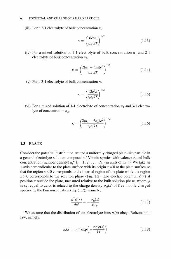
(iii) For a 2-1 electrolyte of bulk concentration n,

k ¼ 6e2n

ereokT

� �1=2

ð1:13Þ

(iv) For a mixed solution of 1-1 electrolyte of bulk concentration n1 and 2-1

electrolyte of bulk concentration n2,

k ¼ 2(n1 þ 3n2)e2

ereokT

� �1=2

ð1:14Þ

(v) For a 3-1 electrolyte of bulk concentration n,

k ¼ 12e2n

ereokT

� �1=2

ð1:15Þ

(vi) For a mixed solution of 1-1 electrolyte of concentration n1 and 3-1 electro-

lyte of concentration n2,

k ¼ 2(n1 þ 6n2)e2

ereokT

� �1=2

ð1:16Þ

1.3 PLATE

Consider the potential distribution around a uniformly charged plate-like particle in

a general electrolyte solution composed of N ionic species with valence zi and bulk

concentration (number density) n1i (i¼ 1, 2, . . . , N) (in units of m�3). We take an

x-axis perpendicular to the plate surface with its origin x¼ 0 at the plate surface so

that the region x< 0 corresponds to the internal region of the plate while the region

x> 0 corresponds to the solution phase (Fig. 1.2). The electric potential c(x) atposition x outside the plate, measured relative to the bulk solution phase, where cis set equal to zero, is related to the charge density rel(x) of free mobile charged

species by the Poisson equation (Eq. (1.2)), namely,

d2c(x)dx2

¼ � rel(x)ereo

ð1:17Þ

We assume that the distribution of the electrolyte ions ni(x) obeys Boltzmann’s

law, namely,

ni(x) ¼ n1i exp � ziec(x)kT

� �ð1:18Þ


where ni(x) is the concentration (number density) of the ith ionic species at position

x. The charge density rel(x) at position x is thus given by

rel(x) ¼XNi¼1

zieni(x) ¼XNi¼1

zien1i exp � ziec(x)

kT

� �ð1:19Þ

Combining Eqs. (1.17) and (1.19) gives the following Poisson–Boltzmann equa-

tion for the potential distribution c(x):

d2c(x)dx2

¼ � 1

ereo

XNi¼1

zien1i exp � ziec(x)

kT

� �ð1:20Þ

We solve the planar Poisson–Boltzmann equation (1.20) subject to the boundary

conditions:

c ¼ co at x ¼ 0 ð1:21Þ

c ! 0;dcdx

! 0 as x ! 1 ð1:22Þ

where co is the potential at the plate surface x¼ 0, which we call the surface

potential.

If the internal electric fields inside the particle can be neglected, then the surface

charge density s of the particle is related to the potential derivative normal to the

Electrolyte

solution

+

+

+

+

+

+

+

+

+

+

+

+

-

-

-

---

-

0

x

ψ(x)

1/κ

Charged

surface

FIGURE 1.2 Schematic representation of potential distribution c(x) near the positively

charged plate.

PLATE 7

particle surface by (see Eq. (1.7))

dcdx

��x¼0þ

¼ � sereo

ð1:23Þ

1.3.1 Low Potential

If the potential c is low (Eq. (1.8)), then Eq. (1.20) reduces to the following linear-

ized Poisson–Boltzmann equation (Eq. (1.9)):

d2cdx2

¼ k2c ð1:24Þ

The solution to Eq. (1.24) subject to Eqs. (1.21) and (1.22) can be easily ob-

tained:

c(x) ¼ coe�kx ð1:25Þ

Equations (1.23) and (1.25) give the following surface charge density–surface

potential (s–co) relationship:

c0 ¼s

ereokð1:26Þ

Equation (1.26) has the following simple physical meaning. Since c decays from

co to zero over a distance of the order of k�1 (Eq. (1.25)), the electric field at the

particle surface is approximately given by co/k�1. This field, which is generated by

s, is equal to s/ereo. Thus, we have co/k�1¼ s/ereo, resulting in Eq. (1.26).

1.3.2 Arbitrary Potential: Symmetrical Electrolyte

Now we solve the original nonlinear Poisson–Boltzmann equation (1.20). If the

plate is immersed in a symmetrical electrolyte of valence z and bulk concentration

n, then Eq. (1.20) becomes

d2c(x)dx2

¼ � zen

ereoexp � zec(x)

kT

� �� exp

zec(x)kT

� ��

¼ 2zen

ereosinh

zec(x)kT

� � ð1:27Þ

We introduce the dimensionless potential y(x)

y ¼ zeckT

ð1:28Þ


then Eq. (1.27) becomes

d2y

dx2¼ k2 sinh y ð1:29Þ

where the Debye–Huckel parameter k is given by Eq. (1.11). Note that y(x) is scaledby kT/ze, which is the thermal energy measured in units of volts. At room tempera-

tures, kT/ze (with z¼ 1) amounts to ca. 25mV. Equation (1.29) can be solved by

multiplying dy/dx on its both sides to give

dy

dx

d2y

dx2¼ k2 sinh y

dy

dxð1:30Þ

which is transformed into

1

2

d

dx

dy

dx

� �2( )

¼ k2d

dxcosh y ð1:31Þ

Integration of Eq. (1.31) gives

dy

dx

� �2

¼ 2k2 cosh yþ constant ð1:32Þ

By taking into account Eq. (1.22), we find that constant¼�2k2 so that Eq.

(1.32) becomes

dy

dx

� �2

¼ 2k2(cosh y� 1) ¼ 4k2 sinh2y

2

� �ð1:33Þ

Since y and dy/dx are of opposite sign, we obtain from Eq. (1.33)

dy

dx¼ �2k sinh(y=2) ð1:34Þ

Equation (1.34) can be further integrated to give

Z yo

y

dy

2 sinh(y=2)¼ k

Z x

0

dx ð1:35Þ

where

yo ¼zeco

kTð1:36Þ

PLATE 9

is the scaled surface potential. Thus, we obtain

y(x) ¼ 4 arctanh(ge�kx) ¼ 2 ln1þ ge�kx

1� ge�kx

� �ð1:37Þ

or

c(x) ¼ 2kT

zeln

1þ ge�kx

1� ge�kx

� �ð1:38Þ

with

g ¼ tanhzeco

4kT

� �¼ exp(zeco=2kT)� 1

exp(zeco=2kT)þ 1¼ exp(yo=2)� 1

exp(yo=2)þ 1ð1:39Þ

Figure 1.3 exhibits g as a function of yo, showing that g is a linearly increasing

function of yo for low yo, namely,

g � yo4¼ zeco

4kTð1:40Þ

but reaches a plateau value at 1 for jyoj � 8.

Figure 1.4 shows y(x) for several values of yo calculated from Eq. (1.37) in compar-

ison with the Debye–Huckel linearized solution (Eq. (1.25)). It is seen that the Debye–

Huckel approximation is good for low potentials (|yo|� 1). As seen from Eqs. (1.25)

and (1.37), the potential c(x) across the electrical double layer varies nearly

FIGURE 1.3 g as a function of jyoj (Eq. (1.39)).


exponentially (Eqs. (1.37)) or exactly exponentially (Eq. (1.25)) with the distance xfrom the plate surface, as shown in Fig. 1.4. Equation (1.25) shows that the potential

c(x) decays from co at x¼ 0 to co/e (co/3) at x¼ 1/k. Thus, the reciprocal of the

Debye–Huckel parameter k (the Debye length), which has the dimension of length,

serves as a measure for the thickness of the electrical double layer. Figure 1.5 plots the

FIGURE 1.5 Concentrations of counterions (anions) n�(x) and coions (cations) n+(x)around a positively charged planar surface (arbitrary scale). Calculated from Eqs. (1.3) and

(1.26) for yo¼ 2.

FIGURE 1.4 Potential distribution y(x)� zec(x)/kT around a positively charged plate

with scaled surface potential yo� zeco/kT. Calculated for yo¼ 1, 2, and 4. Solid lines, exact

solution (Eq. (1.37)); dashed lines, the Debye–Huckel linearized solution (Eq. (1.25)).

PLATE 11

concentrations of counterion (n�(x)¼ n exp(y(x))) and coions (nþ(x)¼ n exp(�y(x)))around a positively charged plate as a function of the distance x from the plate surface,

showing that these quantities decay almost exponentially over the distance of the

Debye length 1/k just like the potential distribution c(x) in Fig. 1.4.By substituting Eq. (1.38) into Eq. (1.23), we obtain the following relationship

connecting co and s:

s ¼ 2ereokkTze

sinhzeco

2kT

� �¼ (8nereokT)1=2 sinh

zeco

2kT

� �ð1:41Þ

or inversely,

co ¼ 2kT

zearcsinh

sffiffiffiffiffiffiffiffiffiffiffiffiffiffiffiffiffiffi8nereokT

p� �

¼ 2kT

zearcsinh

zes2ereokkT

� �

¼ 2kT

zeln

zes2ereokkT

þ zes2ereokkT

� �2

þ 1

( )" # ð1:42Þ

If s is small and thus co is low, that is, the condition (Eq. (1.8)) is fulfilled, then

Eq. (1.38) reduces to Eq. (1.25) with the surface potential given by Eq. (1.26). Fig-

ure 1.6 shows the s–co relationship calculated from Eq. (1.42) in comparison with

the approximate results (Eq. (1.26)). The deviation of Eq. (1.26) from Eq. (1.42)

becomes significant as the charge density s increases.

FIGURE 1.6 Scaled surface potential yo¼ zeco/kT as a function of the scaled surface

charge density s�¼ zes/ereokkT for a positively charged planar plate in a symmetrical elec-

trolyte solution of valence z. Solid line, exact solution (Eq. (1.41)); dashed line, Debye–

Huckel linearized solution (Eq. (1.26)).


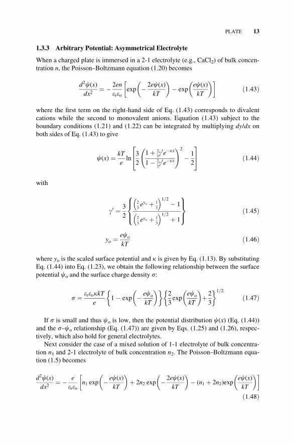
1.3.3 Arbitrary Potential: Asymmetrical Electrolyte

When a charged plate is immersed in a 2-1 electrolyte (e.g., CaCl2) of bulk concen-

tration n, the Poisson–Boltzmann equation (1.20) becomes

d2c(x)dx2

¼ � 2en

ereoexp � 2ec(x)

kT

� �� exp

ec(x)kT

� �� ð1:43Þ

where the first term on the right-hand side of Eq. (1.43) corresponds to divalent

cations while the second to monovalent anions. Equation (1.43) subject to the

boundary conditions (1.21) and (1.22) can be integrated by multiplying dy/dx on

both sides of Eq. (1.43) to give

c(x) ¼ kT

eln

3

2

1þ 2

3g0e�kx

1� 2

3g0e�kx

!2

� 1

2

24

35 ð1:44Þ

with

g0 ¼ 3

2

2

3eyo þ 1

3

� �1=2� 1

2

3eyo þ 1

3

� �1=2þ 1

8><>:

9>=>; ð1:45Þ

yo ¼eco

kTð1:46Þ

where yo is the scaled surface potential and k is given by Eq. (1.13). By substituting

Eq. (1.44) into Eq. (1.23), we obtain the following relationship between the surface

potential co and the surface charge density s:

s ¼ ereokkTe

1� exp � eco

kT

� � 2

3exp

eco

kT

� �þ 2

3

1=2

ð1:47Þ

If s is small and thus co is low, then the potential distribution c(x) (Eq. (1.44))and the s–co relationship (Eq. (1.47)) are given by Eqs. (1.25) and (1.26), respec-

tively, which also hold for general electrolytes.

Next consider the case of a mixed solution of 1-1 electrolyte of bulk concentra-

tion n1 and 2-1 electrolyte of bulk concentration n2. The Poisson–Boltzmann equa-

tion (1.5) becomes

d2c(x)dx2

¼ � e

ereon1 exp � ec(x)

kT

� �þ 2n2 exp � 2ec(x)

kT

� �� (n1 þ 2n2)exp

ec(x)kT

� �� ð1:48Þ

PLATE 13

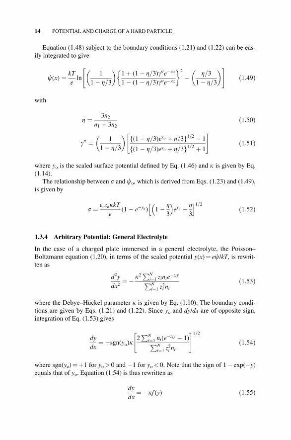
Equation (1.48) subject to the boundary conditions (1.21) and (1.22) can be eas-

ily integrated to give

c(x) ¼ kT

eln

1

1� Z=3

� �1þ (1� Z=3)g00e�kx

1� (1� Z=3)g00e�kx

2

� Z=31� Z=3

� �" #ð1:49Þ

with

Z ¼ 3n2n1 þ 3n2

ð1:50Þ

g00 ¼ 1

1� Z=3

� � f(1� Z=3)eyo þ Z=3g1=2 � 1

f(1� Z=3)eyo þ Z=3g1=2 þ 1

" #ð1:51Þ

where yo is the scaled surface potential defined by Eq. (1.46) and k is given by Eq.

(1.14).

The relationship between s and co, which is derived from Eqs. (1.23) and (1.49),

is given by

s ¼ ereokkTe

(1� e�yo ) 1� Z3

� �eyo þ Z

3

h i1=2ð1:52Þ

1.3.4 Arbitrary Potential: General Electrolyte

In the case of a charged plate immersed in a general electrolyte, the Poisson–

Boltzmann equation (1.20), in terms of the scaled potential y(x)¼ ec/kT, is rewrit-ten as

d2y

dx2¼ � k2

PNi¼1 zinie

�ziyPNi¼1 z

2i ni

ð1:53Þ

where the Debye–Huckel parameter k is given by Eq. (1.10). The boundary condi-

tions are given by Eqs. (1.21) and (1.22). Since yo and dy/dx are of opposite sign,

integration of Eq. (1.53) gives

dy

dx¼ �sgn(yo)k

2PN

i¼1 ni(e�ziy � 1)PN

i¼1 z2i ni

" #1=2ð1:54Þ

where sgn(yo)¼þ1 for yo> 0 and �1 for yo< 0. Note that the sign of 1� exp(�y)equals that of yo. Equation (1.54) is thus rewritten as

dy

dx¼ �kf (y) ð1:55Þ


with

f (y) ¼ sgn(yo)2PN


i¼1 z2i ni

" #1=2¼ (1� e�y)

2PN

i¼1 ni(e�ziy � 1)

(1� e�y)2PN

i¼1 z2i ni

" #1=2

ð1:56ÞNote that as y! 0, f(y)! y. Explicit expressions for f(y) for some simple cases

are given below.

(i) For a symmetrical electrolyte of valence z,

f (y) ¼ 2 sinh(zy=2) ð1:57Þ

(ii) For a monovalent electrolyte,

f (y) ¼ 2 sinh(y=2) ð1:58Þ

(iii) For a 2-1 electrolyte,

f (y) ¼ (1� e�y)2

3ey þ 1

3

� �1=2

ð1:59Þ

(iv) For a mixed solution of 2-1 electrolyte of concentration n2 and 1-1 electro-


f (y) ¼ (1� e�y) 1� Z3

� �ey þ Z

3

h i1=2ð1:60Þ

with

Z ¼ 3n2n1 þ 3n2

ð1:61Þ

(v) For a 3-1 electrolyte,

f (y) ¼ (1� e�y)1

2ey þ 1

3þ 1

6e�y

� �1=2

ð1:62Þ

(vi) For a mixed solution of 3-1 electrolyte of concentration n2 and 1-1 electro-


f (y) ¼ (1� e�y) 1� Z0

2

� �ey þ Z0

3þ Z0

6e�y

� �1=2ð1:63Þ

PLATE 15

with

Z0 ¼ 6n2n1 þ 6n2

ð1:64Þ

By integrating Eq. (1.55) between x¼ 0 (y¼ yo) and x¼ x (y¼ y), we obtain

kx ¼Z yo

y

dy

f (y)ð1:65Þ

which gives the relationship between y and x. For a symmetrical electrolyte of va-

lence z, 2-1 electrolytes, and a mixed solution of 2-1 electrolyte of concentration n2and 1-1 electrolyte of concentration n1, Eq. (1.65) reproduces Eqs. (1.38), (1.44),and (1.49), respectively.

The surface charge density–surface potential (s–yo) relationship is obtained fromEqs. (1.23) and (1.55) and given in terms of f(yo) as

s ¼ �ereodcdx

��x¼0þ

¼ ereokkTe

f (yo) ð1:66Þ

or

s ¼ ere0kkTe

sgn(yo)

2XNi¼1

ni(e�ziy0 � 1)

XNi¼1

z3i ni

266664

377775

1=2

¼ ere0kkTe

sgn(yo)(1� e�y0 )

2XNi¼1

ni(e�ziy0 � 1)

(1� e�y0 )2XNi¼1

z2i ni

266664

377775

1=2ð1:67Þ

Note that as yo! 0, f(yo)! yo so that for low yo Eq. (1.67) reduces to Eq. (1.26).For a symmetrical electrolyte of valence z, 2-1 electrolytes, and a mixed solution of

2-1 electrolyte of concentration n2 and 1-1 electrolyte of concentration n1, Eq.(1.67) combined with Eqs. (1.57), (1.59), and (1.60) reproduces Eqs. (1.41), (1.47),

and (1.52), respectively.

1.4 SPHERE

Consider a spherical particle of radius a in a general electrolyte solution. The

electric potential c(r) at position r obeys the following spherical Poisson–

Boltzmann equation [3]:

d2cdr2

þ 2

r

dcdr

¼ � 1

ereo

XNi¼1

zien1i exp � ziec

kT

� �ð1:68Þ


where we have taken the spherical coordinate system with its origin r¼ 0 placed

at the center of the sphere and r is the distance from the center of the particle

(Fig. 1.7). The boundary conditions for c(r), which are similar to Eqs. (1.21)

and (1.22) for a planar surface, are given by

c ¼ co at r ¼ aþ ð1:69Þ

c ! 0;dcdr

! 0 as zr ! 1 ð1:70Þ

1.4.1 Low Potential

When the potential is low, Eq. (1.68) can be linearized to give

d2cdr2

þ 2

r

dcdr

¼ k2c ð1:71Þ

The solution to Eq. (1.71) subject to Eqs. (1.69) and (1.70) is

c(r) ¼ co

a

re�k(r�a) ð1:72Þ

If we introduce the distance x¼ r� ameasured from the sphere surface, then Eq.

(1.72) becomes

c(x) ¼ co

a

aþ xe�kx ð1:73Þ

For x � a, Eq. (1.73) reduces to the potential distribution around the planar sur-

face given by Eq. (1.19). This result implies that in the region very near the particle

surface, the surface curvature may be neglected so that the surface can be regarded

as planar. In the limit of k! 0, Eq. (1.72) becomes

c(r) ¼ co

a

rð1:74Þ

FIGURE 1.7 A sphere of radius a.

SPHERE 17

which is the Coulomb potential distribution around a sphere as if there were no

electrolyte ions or electrical double layers. Note that Eq. (1.74) implies that the po-

tential decays over distances of the particle radius a, instead of the double layer

thickness 1/k.The surface charge density s of the particle is related to the particle surface po-

tential co obtained from the boundary condition at the sphere surface,

@c@r

��r¼aþ

¼ � sereo

ð1:75Þ

which corresponds to Eq. (1.23) for a planar surface. By substituting Eq. (1.72) into

Eq. (1.75), we find the following co–s relationship:

co ¼s

ereok(1þ 1=ka)ð1:76Þ

For ka � 1, Eq. (1.76) tends to Eq. (1.26) for the co–s relationship for the plate

case. That is, for ka � 1, the curvature of the particle surface may be neglected so

that the particle surface can be regarded as planar. In the opposite limit of ka � 1,

Eq. (1.76) tends to

co ¼saereo

ð1:77Þ

If we introduce the total charge Q¼ 4pa2 on the particle surface, then Eq. (1.77)

can be rewritten as

co ¼Q

4pereoað1:78Þ

which is the Coulomb potential. This implies that for ka � 1, the existence of

the electrical double layer may be ignored. Figures 1.8 and 1.9, respectively, show

that Eq. (1.76) tends to Eq. (1.26) for a planar co–s relationship for ka � 1 and to

the Coulomb potential given by Eq. (1.78) for ka � 1. It is seen that the surface

potential co of a spherical particle of radius a can be regarded as co of a plate for

ka� 102 (Fig. 1.8) and as the Coulomb potential for ka� 10�2 (Fig. 1.9). That is,

for ka� 10�2, the presence of the electrical double layer can be neglected.

1.4.2 Surface Charge Density–Surface Potential Relationship: SymmetricalElectrolyte

When the magnitude of the surface potential is arbitrary so that the Debye–Huckel

linearization cannot be allowed, we have to solve the original nonlinear spherical

Poisson–Boltzmann equation (1.68). This equation has not been solved but its approxi-

mate analytic solutions have been derived [5–8]. Consider a sphere of radius a with a


surface charge density s immersed in a symmetrical electrolyte solution of valence zand bulk concentration n. Equation (1.68) in the present case becomes

d2cdr2

þ 2

r

dcdr

¼ 2zen

ereosinh

zeckT

� �ð1:79Þ

FIGURE 1.8 Surface potential co and surface charge density s relationship of a spherical

particle of radius a as a function of ka calculated with Eq. (1.76). For ka� 102, the surface

potential co can be regarded as co = s/ereok for the surface potential of a plate.

FIGURE 1.9 Surface potential co and surface charge density s relationship of a spherical

particle of radius a as a function of ka calculated with Eq. (1.76). For ka� 10�2, the surface

potential co can be regarded as the Coulomb potential co =Q/4pereoa.

SPHERE 19

Loeb et al. tabulated numerical computer solutions to the nonlinear spherical

Poisson–Boltzmann equation (1.63). On the basis of their numerical tables, they

discovered the following empirical formula for the s–co relationship:

s ¼ 2ereokkTze

sinhzeco

2kT

� �þ 2

ka

� �tanh

zeco

4kT

� �� ð1:80Þ

where the Debye–Huckel parameter k is given by Eq. (1.11). A mathematical

basis of Eq. (1.80) was given by Ohshima et al. [7], who showed that if, on the

left-hand side of Eq. (1.79), we replace 2/r with its large a limiting form 2/a and

dc/dr with that for a planar surface (the zeroth-order approximation given by

Eq. (1.34)), namely,

2

r

dcdr

! 2

a

dcdr

��zeroth-order

¼ � 4kasinh

zec2kT

� �ð1:81Þ

then Eq. (1.63) becomes

d2y

dr2¼ k2

�sinhyþ 4

kasinh

y

2

� ��ð1:82Þ

where y¼ zec/kT is the scaled potential (Eq. (1.28)). Since the right-hand side

of Eq. (1.82) involves only y (and does not involve r explicitly), Eq. (1.82) canbe readily integrated by multiplying dy/dr on its both sides to yield

dy

dr¼ �2k sinh

y

2

� �1þ 2

ka cosh2(y=4)

� �1=2ð1:83Þ

By expanding Eq. (1.83) with respect to 1/ka and retaining up to the first order of1/ka, we obtain

dy

dr¼ �2k sinh

y

2

� �1þ 1

ka cosh2(y=4)

� �ð1:84Þ

Substituting Eq. (1.84) into Eq. (1.75), we obtain Eq. (1.80), which is the first-

order s–co relationship.

A more accurate s–co relationship can be obtained by using the first-order ap-

proximation given by Eq. (1.84) (not using the zeroth-order approximation for a

planar surface given by Eq. (1.34)) in the replacement of Eq. (1.81), namely,

2

r

dy

dr! 2

a

dy

dr

��first-order

¼ � 4

ak sinh

y

2

� �1þ 1

ka cosh2(y=4)

� �ð1:85Þ


The result is

s ¼ 2ereokkTze

sinhzeco

2kT

� �1þ 1

ka2

cosh2(zeco=4kT)þ 1

(ka)28ln[cosh(zeco=4kT)]

sinh2(zeco=2kT)

� �1=2ð1:86Þ

which is the second-order s–co relationship [4]. The relative error of Eq. (1.80) is

less than 1% for ka� 5 and that of Eq. (1.86) is less than 1% for ka� 1. Note that

as yo increases, Eqs. (1.80) and (1.86) approach Eq. (1.41). That is, as the surface

potential yo increases, the dependence of yo on ka becomes smaller. Figure 1.10

gives the s–co relationship for various values of ka calculated from Eq. (1.86) in

comparison with the low-potential approximation (Eq. (1.76)).

1.4.3 Surface Charge Density–Surface Potential Relationship: AsymmetricalElectrolyte

The above approximation method can also be applied to the case of a sphere in a 2-1

symmetrical solution, yielding [4]

s ¼ ereokkTe

pqþ 2f(3� p)q� 3gkapq

� �ð1:87Þ

FIGURE 1.10 Scaled surface charge density s�= zes/ereokkT as a function of the scaled

surface potential yo = zeco/kT for a positively charged sphere in a symmetrical electrolyte

solution of valence z for various values of ka. Solid line, exact solution (Eq. (1.86)); dashed

line, Debye–Huckel linearized solution (Eq. (1.76)).

SPHERE 21

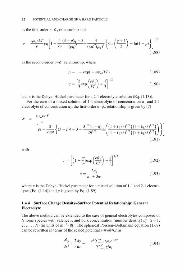
as the first-order s–co relationship and

s ¼ ereokkTe

pq 1þ 4

ka(3� p)q� 3

(pq)2

�þ 4

(ka)2(pq)26ln

qþ 1

2

� �þ ln(1� p)

�1=2ð1:88Þ

as the second-order s–co relationship, where

p ¼ 1� exp(� eco=kT) ð1:89Þ

q ¼ 2

3exp

eco

kT

� �þ 1

3

� �1=2ð1:90Þ

and k is the Debye–Huckel parameter for a 2-1 electrolyte solution (Eq. (1.13)).

For the case of a mixed solution of 1-1 electrolyte of concentration n1 and 2-1

electrolyte of concentration n2, the first-order s–co relationship is given by [7]

s ¼ ereokkTe

pt þ 2

kapt(3� p)t � 3� 31=2(1� Z)

2Z1=2

�ln

f1þ (Z=3)1=2gft � (Z=3)1=2gf1� (Z=3)1=2gft þ (Z=3)1=2g

!)#

ð1:91Þ

with

t ¼ 1� Z3

� �exp

eco

kT

� �þ Z3

� �1=2ð1:92Þ

Z ¼ 3n2n1 þ 3n2

ð1:93Þ

where k is the Debye–Huckel parameter for a mixed solution of 1-1 and 2-1 electro-

lytes (Eq. (1.14)) and p is given by Eq. (1.89).

1.4.4 Surface Charge Density–Surface Potential Relationship: GeneralElectrolyte

The above method can be extended to the case of general electrolytes composed of

N ionic species with valence zi and bulk concentration (number density) n1i (i¼ 1,

2, . . . , N) (in units of m�3) [8]. The spherical Poisson–Boltzmann equation (1.68)

can be rewritten in terms of the scaled potential y� ec/kT as

d2y

dr2þ 2

r

dy

dr¼ � k2

PNi¼1 zinie

�ziyPNi¼1 z

2i ni

ð1:94Þ


where k is the Debye–Huckel parameter of the solution and defined by Eq. (1.10).

In the limit of large ka, Eq. (1.94) reduces to the planar Poisson–Boltzmann

equation (1.53), namely,

d2y

dr2¼ � k2

PNi¼1 zinie

�ziyPNi¼1 z

2i ni

ð1:95Þ

Integration of Eq. (1.95) gives

dy

dr¼ �sgn(yo)k

2PN


i¼1 z2i ni

" #1=2ð1:96Þ

Equation (1.96) is thus rewritten as

dy

dr¼ �kf (y) ð1:97Þ

where f(y) is defined by Eq. (1.56). Note that as y! 0, f(y) tends to y and the right--hand side of Eq. (1.94) is expressed as k2f(y)df/dy. By combining Eqs. (1.75) and

(1.97), we obtain

s ¼ �ereodcdr

��r¼aþ

¼ ereokkTe

f (yo) ð1:98Þ

where yo� ec/kT is the scaled surface potential. Equation (1.98) is the zeroth-order

s–yo relationship.To obtain the first-order s–yo relationship, we replace the second term on the

left-hand side of Eq. (1.94) by the corresponding quantity for the planar case (Eq.

(1.88)), namely,

2

r

dy

dr! 2

a

dy

dr

��zeroth-order

¼ � 2kaf (y) ð1:99Þ

Equation (1.94) thus becomes

d2y

dr2¼ 2k

af (y)þ k2f (y)

df

dyð1:100Þ

which is readily integrated to give

dy

dr¼ �kf (y) 1þ 4

kaf 2(y)

Z y

0

f (u)du

� �1=2ð1:101Þ

SPHERE 23

By expanding Eq. (1.101) with respect to 1/ka and retaining up to the first order

of 1/ka, we have

dy

dr¼ �kf (y) 1þ 2

kaf 2(y)

Z y

0

f (u)du

� �ð1:102Þ

From Eqs. (1.75) and (1.102) we obtain the first-order s–yo relationship, namely,

s ¼ ereokkTe

f (yo) 1þ 2

kaf 2(yo)

Z yo

0

f (u)du

� �ð1:103Þ

Note that since f(yo)! yo as yo! 0, Eq. (1.103) tends to the correct form in the

limit of small yo (Eq. (1.76)), namely,

s ¼ ereok 1þ 1

ka

� �co ð1:104Þ

We can further obtain the second-order s–yo relationship by replacing the secondterm on the left-hand side of Eq. (1.94) by the corresponding quantity for the first-

order case (i.e., by using Eq. (1.101) instead of Eq. (1.97)), namely,

2

r

dy

dr! 2

a

dy

dr

��first-order

¼ � 2kaf (y) 1þ 2

lkaf 2(y)

Z y

0

f (u)du

� �ð1:105Þ

where we have introduced a fitting parameter l. Then, Eq. (1.94) becomes

d2y

dr2¼ 2k

af (y) 1þ 2

lkaf 2(y)

Z y

0

f (u)du

� �þ k2f (y)

df

dyð1:106Þ

which is integrated to give

s ¼ ereokkTe

f (yo) 1þ 4

kaf 2(yo)

Z yo

0

f (y)dy

�þ 8

l(ka)2f 2(yo)

Z yo

0

1

f (y)

Z y

0

f (u)du

dy

�1=2ð1:107Þ

In the limit of small yo, Eq. (1.107) tends to

s ¼ ereokco 1þ 2

kaþ 2

l(ka)2

� �1=2ð1:108Þ


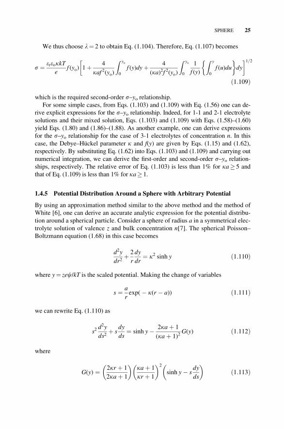
We thus choose l¼ 2 to obtain Eq. (1.104). Therefore, Eq. (1.107) becomes

s ¼ ereokkTe

f (yo) 1þ 4

kaf 2(yo)

Z yo

0

f (y)dy

�þ 4

(ka)2f 2(yo)

Z yo

0

1

f (y)

Z y

0

f (u)du

dy

�1=2ð1:109Þ

which is the required second-order s–yo relationship.For some simple cases, from Eqs. (1.103) and (1.109) with Eq. (1.56) one can de-

rive explicit expressions for the s–yo relationship. Indeed, for 1-1 and 2-1 electrolyte

solutions and their mixed solution, Eqs. (1.103) and (1.109) with Eqs. (1.58)–(1.60)

yield Eqs. (1.80) and (1.86)–(1.88). As another example, one can derive expressions

for the s–yo relationship for the case of 3-1 electrolytes of concentration n. In this

case, the Debye–Huckel parameter k and f(y) are given by Eqs. (1.15) and (1.62),

respectively. By substituting Eq. (1.62) into Eqs. (1.103) and (1.109) and carrying out

numerical integration, we can derive the first-order and second-order s–yo relation-ships, respectively. The relative error of Eq. (1.103) is less than 1% for ka� 5 and

that of Eq. (1.109) is less than 1% for ka� 1.

1.4.5 Potential Distribution Around a Sphere with Arbitrary Potential

By using an approximation method similar to the above method and the method of

White [6], one can derive an accurate analytic expression for the potential distribu-

tion around a spherical particle. Consider a sphere of radius a in a symmetrical elec-

trolyte solution of valence z and bulk concentration n[7]. The spherical Poisson–

Boltzmann equation (1.68) in this case becomes

d2y

dr2þ 2

r

dy

dr¼ k2 sinh y ð1:110Þ

where y¼ zec/kT is the scaled potential. Making the change of variables

s ¼ a

rexp(� k(r � a)) ð1:111Þ

we can rewrite Eq. (1.110) as

s2d2y

ds2þ s

dy

ds¼ sinh y� 2kaþ 1

(kaþ 1)2G(y) ð1:112Þ

where

G(y) ¼ 2kr þ 1

2kaþ 1

� �kaþ 1

kr þ 1

� �2

sinh y� sdy

ds

� �ð1:113Þ

SPHERE 25

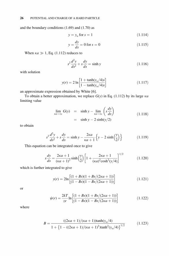
and the boundary conditions (1.69) and (1.70) as

y ¼ yo for s ¼ 1 ð1:114Þ

y ¼ dy

ds¼ 0 for s ¼ 0 ð1:115Þ

When ka � 1, Eq. (1.112) reduces to

s2d2y

ds2þ s

dy

ds¼ sinh y ð1:116Þ

with solution

y(r) ¼ 2 ln1þ tanh(yo=4)s

1� tanh(yo=4)s

� �ð1:117Þ

an approximate expression obtained by White [6].

To obtain a better approximation, we replace G(y) in Eq. (1.112) by its large kalimiting value

limka!1G(y) ¼ sinh y� lim

ka!1 sdy

ds

� �¼ sinh y� 2 sinh(y=2)

ð1:118Þ

to obtain

s2d2y

ds2þ s

dy

ds¼ sinh y� 2ka

kaþ 1y� 2 sinh

y

2

� �n oð1:119Þ

This equation can be integrated once to give

sdy

ds¼ 2kaþ 1

(kaþ 1)2sinh

y

2

� �1þ 2kaþ 1

(ka)2cosh2(y=4)

� �1=2ð1:120Þ

which is further integrated to give

y(r) ¼ 2ln(1þ Bs)(1þ Bs=(2kaþ 1))

(1� Bs)(1� Bs=(2kaþ 1))

� �ð1:121Þ

or

c(r) ¼ 2kT

zeln

(1þ Bs)(1þ Bs=(2kaþ 1))

(1� Bs)(1� Bs=(2kaþ 1))

� �ð1:122Þ

where

B ¼ ((2kaþ 1)=(kaþ 1))tanh(yo=4)

1þ 1� ((2kaþ 1)=(kaþ 1)2)tanh2(yo=4)� �1=2 ð1:123Þ


The relative error of Eq. (1.122) is less than 1% for ka� 1. Note also that Eq.

(1.121) or (1.122) exhibits the correct asymptotic form, namely,

y(r) ¼ costant s ð1:124Þ

Figure 1.11 gives the scaled potential distribution y(r) around a positively

charged spherical particle of radius a with yo¼ 2 in a symmetrical electrolyte solu-

tion of valence z for several values of ka. Solid lines are the exact solutions to Eq.

(1.110) and dashed lines are the Debye–Huckel linearized results (Eq. (1.72)). Note

that Eq. (1.122) is in excellent agreement with the exact results. Figure 1.12 shows

the plot of the equipotential lines around a sphere with yo¼ 2 at ka¼ 1 calculated

from Eq. (1.121). Figures 1.13 and 1.14, respectively, are the density plots of coun-

terions (anions) (n_(r)¼ n exp(þy(r))) and coions (cations) (nþ(r)¼ n exp(�y(r)))around the sphere calculated from Eq. (1.121).

Note that one can obtain the s–yo relationship from Eq. (1.120),

s ¼ �ereody

dr

��r¼aþ

¼ ereokkTe

kaþ 1

kasdy

ds

��s¼1

¼ 2ereokkTe

sinhyo2

� �1þ 2kaþ 1

(ka)2cosh2(yo=4)

� �1=2 ð1:125Þ

FIGURE 1.11 Scaled potential distribution y(r) around a positively charged spherical par-ticle of radius a with yo¼ 2 in a symmetrical electrolyte solution of valence z for severalvalues of ka. Solid lines, exact solution to Eq. (1.110); dashed lines, Debye–Huckel linear-

ized solution (Eq. (1.72)). Note that the results obtained from Eq. (1.122) agree with the exact

results within the linewidth.

SPHERE 27

FIGURE 1.13 Density plots of counterions (anions) around a positively charged spherical

particle with yo¼ 2 at ka¼ 1. Calculated from n�(r)¼ n exp(+y(r)) with the help of Eq.

(1.121). The darker region indicates the higher density and n�(r) tends to its bulk value n far

from the particle. Arbitrary scale.

FIGURE 1.12 Contour lines (isopotential lines) for c(r) around a positively charged

sphere with yo¼ 2 at ka¼ 1. Arbitrary scale.


which corresponds to Eq. (1.80), but one cannot derive the second-order s–yorelationship by this method. The advantage in transforming the spherical Poisson–

Boltzmann equation (1.79) into Eq. (1.112) lies in its ability to yield the potential

distribution y(r) that shows the correct asymptotic form (Eq. (1.124)).

We obtain the potential distribution around a sphere of radius a having a surface

potential co immersed in a solution of general electrolytes [9]. The Poisson–

Boltzmann equation for the electric potential c(r) is given by Eq. (1.94), which, in

terms of f(r), is rewritten as

d2y

dr2þ 2

r

dy

dr¼ k2f (y)

dy

drð1:126Þ

with f(r) given by Eq. (1.56). We make the change of variables (Eq. (1.111)) and

rewrite Eq. (1.126) as

s2d2y

ds2þ s

dy

ds¼ f (y)

df

dy� 2kr þ 1

(kr þ 1)2f (y)

df

dy� s

dy

ds

ð1:127Þ

which is subject to the boundary conditions: y¼ yo at s¼ 1 and y¼ dy/ds¼ 0 at

s¼ 0 (see Eqs. (1.114) and (1.115)). When ka � 1, Eq. (1.127) reduces to

s2d2y

ds2þ s

dy

ds¼ f (y)

df

dyð1:128Þ

FIGURE 1.14 Density plots of coions (cations) around a positively charged spherical par-

ticle with yo¼ 2 at ka¼ 1. Calculated from n+(r)¼ n exp(�y(r)) with the help of Eq. (1.121).

The darker region indicates the higher density and n+(r) tends to its bulk value n far from the

particle.

SPHERE 29

which is integrated once to give

sdy

ds¼ f (y) ð1:129Þ

We then replace the second term on the right-hand side of Eq. (1.127) with its

large ka limiting form, that is, kr! ka and s dy/ds! f(y) (Eq. (1.120)),

2kr þ 1

(kr þ 1)2f (y)

df

dy� s

dy

ds

! 2kaþ 1

(kaþ 1)2f (y)

df

dy� f (y)

ð1:130Þ

Equation (1.127) then becomes

s2d2y

ds2þ s

dy

ds¼ þf (y)

df

dy� 2kaþ 1

(kaþ 1)2f (y)

df

dy� s

dy

ds

ð1:131Þ

and integrating the result once gives

sdy

ds¼ F(y) ð1:132Þ

with

F(y) ¼ kakaþ 1

f (y) 1þ 2(2kaþ 1)

(ka)21

f 2(y)

Z y

0

f (u)du

� �1=2ð1:133Þ

Note that F(y)! y as y! 0 and that F(y)! f(y) as ka!1. Expressions for F(y) for several cases are given below.

(i) For a 1-1 electrolyte solution,

F(y) ¼ 2kakaþ 1

sinhy

2

� �1þ 2(2kaþ 1)

(ka)21

cosh2(y=4)

� �1=2ð1:134Þ

(ii) For the case of 2-1 electrolytes,

F(y) ¼ kakaþ 1

(1� e�y)2

3ey þ 1

3

� �1=2

1þ 2(2kaþ 1)(2þ e�y)(23ey þ 1

3)1=2�3

(ka)2(1�e�y)

2(23ey þ 1

3)

" #1=2 ð1:135Þ


(iii) For the case of a mixed solution of 1-1 electrolyte of concentration n1 and2-1 electrolyte of concentration n2,

F(y) ¼ kakaþ 1

(1� e�y) 1� Z3

� �ey þ Z

3

h i1=2 1þ 2(2kaþ 1)

(ka)2(1� e�y)2f(1� Z=3)ey þ Z=3g

�

(2þ e�y)

ffiffiffiffiffiffiffiffiffiffiffiffiffiffiffiffiffiffiffiffiffiffiffiffiffiffiffiffiffi1� Z

3

� �ey þ Z

3

r� 3�

ffiffiffi3

p(1� Z)2ffiffiffiZ

p

lnf ffiffiffiffiffiffiffiffiffiffiffiffiffiffiffiffiffiffiffiffiffiffiffiffiffiffiffiffiffiffiffiffiffiffiffiffi

(1� Z=3)ey þ Z=3p � ffiffiffiffiffiffiffiffi

Z=3p g(1þ ffiffiffiffiffiffiffiffi

Z=3p

)

f ffiffiffiffiffiffiffiffiffiffiffiffiffiffiffiffiffiffiffiffiffiffiffiffiffiffiffiffiffiffiffiffiffiffiffiffi(1� Z=3)ey þ Z=3

p þ ffiffiffiffiffiffiffiffiZ=3

p g(1� ffiffiffiffiffiffiffiffiZ=3

p)

!)#1=2

ð1:136Þ

where Z is defined by Eq. (1.61).

Equation (1.132) is integrated again to give

�ln s ¼Z yo

y

dy

F(y)ð1:137Þ

Substituting Eq. (1.134) into Eq. (1.137), we obtain Eq. (1.122) with z¼ 1. For a

2-1 electrolyte and a mixture of 1-1 and 2-1 electrolytes, one can numerically calcu-

late y(r) from Eq. (1.137) with the help of Eqs. (1.135) and (1.136) for F(y). For a3-1 electrolyte and a mixture of 1-1 and 3-1 electrolytes, one can numerically calcu-

late F(y) from f(y) (Eqs. (1.62) and (1.63)) with the help of Eq. (1.133) and then

calculate y(r) from Eq. (1.137).

1.5 CYLINDER

A similar approximation method can be applied for the case of infinitely long cylin-

drical particles of radius a in a general electrolyte composed of N ionic species with

valence zi and bulk concentration ni (i ¼ 1, 2, . . . , N). The cylindrical Poisson–

Boltzmann equation is

d2cdr2

þ 1

r

dcdr

¼ � 1

ereo

XNi¼1

zien1i exp � ziec

kT

� �ð1:138Þ

where r is the radial distance measured from the center of the cylinder (Fig. 1.15).

The conditions (1.69), (1.70), and (1.75) for a spherical particle of radius a are also

CYLINDER 31

applied for a cylindrical particle of radius a, namely,

c ¼ co at r ¼ aþ ð1:139Þ

c ! 0;dcdr

! 0 as r ! 1 ð1:140Þ

@c@r

��r¼aþ

¼ � sereo

ð1:141Þ

where s is the surface charge density of the cylinder.

1.5.1 Low Potential

For low potentials, Eq. (1.128) reduces to

d2cdr2

þ 1

r

dcdr

¼ k2c ð1:142Þ

where k is given by Eq. (1.10). The solution is

c(r) ¼ co

K0(kr)K0(ka)

ð1:143Þ

FIGURE 1.15 A cylinder of radius a.


where co is the surface potential of the particle and Kn(z) is the modified Bessel

function of the second kind of order n. The surface charge density s of the particle

is obtained from Eq. (1.141) as

s ¼ ereokco

K1(ka)K0(ka)

ð1:144Þ

or

co ¼s

ereokK0(ka)K1(ka)

ð1:145Þ

In the limit of ka!1, Eq. (1.145) approaches Eq. (1.26) for the plate case.

1.5.2 Arbitrary Potential: Symmetrical Electrolyte

For arbitrary co, accurate approximate analytic formulas have been derived [7,10],

as will be shown below. Consider a cylinder of radius a with a surface charge den-

sity s immersed in a symmetrical electrolyte solution of valence z and bulk concen-

tration n. Equation (1.138) in this case becomes

d2y

dr2þ 1

r

dy

dr¼ k2 sinh y ð1:146Þ

where y¼ zec/kT is the scaled potential. By making the change of variables [6]

c ¼ K0(kr)K0(ka)

ð1:147Þ


c2d2y

dc2þ c

dy

dc¼ sinh y� (1� b2)H(y) ð1:148Þ

where

H(y) ¼ 1� fK0(kr)=K1(kr)g21� b2

" #sinh y� c

dy

dc

� �ð1:149Þ

b ¼ K0(ka)K1(ka)

ð1:150Þ

and the boundary conditions (1.139) and (1.140) as

y ¼ yo for c ¼ 1 ð1:151Þ

y ¼ dy

ds¼ 0 for c ¼ 0 ð1:152Þ

CYLINDER 33

In the limit ka � 1, Eq. (1.148) reduces to

c2d2y

dc2þ c

dy

dc¼ sinh y ð1:153Þ

with solution

y(c) ¼ 2ln1þ tanh(yo=4)c

1� tanh(yo=4)c

� �ð1:154Þ

an expression obtained by White [6]. We note that from Eq. (1.149)

H(y)ka!1

¼ sinh y� 2 sinh(y=2) ð1:155Þ

and replacing H(y) in Eq. (148) by its large ka limiting form (Eq. (1.155)) we obtain

c2d2y

dc2þ c

dy

dc¼ sinh y� (1� b2) sinh y� 2 sinh(y=2)f g ð1:156Þ

This equation can be integrated to give

y(r) ¼ 2 ln(1þ Dc)f1þ ((1� b)=(1þ b))Dcg(1� Dc)f1� ((1� b)=(1þ b))Dcg� �

ð1:157Þ

and

s ¼ 2ereokkTze

sinhyo2

� �1þ 1

b2� 1

� �1

cosh2(yo=4)

� �1=2ð1:158Þ

with

D ¼ 1þ bð Þtanh(yo=4)1þ 1� (1� b2)tanh2(yo=4)

� �1=2 ð1:159Þ

where yo¼ zeco/kT is the scaled surface potential of the cylinder. For low poten-

tials, Eq. (1.158) reduces to Eq. (1.144).

1.5.3 Arbitrary Potential: General Electrolytes

We start with Eq. (1.138), which can be rewritten as

d2y

dr2þ 1

r

dy

dr¼ � k2

PNi¼1 zinie

�ziyPNi¼1 z

2i ni

ð1:160Þ

where y ¼ ec=kT


Equation (1.160) may further be rewritten as

d2y

dr2þ 1

r

dy

dr¼ k2f (y)

df

dyð1:161Þ

where f(y) is defined by Eq. (1.56). Making the change of variables (Eq. (1.147)),


c2d2y

dc2þ c

dy

dc¼ f (y)

df

dy� 1� K0(kr)

K1(kr)

2" #

f (y)df

dy� c

dy

dc

ð1:162Þ

When ka � 1, Eq. (1.162) reduces to

c2d2y

dc2þ c

dy

dc¼ f (y)

df

dyð1:163Þ

Equation (1.163) is integrated once to give

cdy

dc¼ f (y) ð1:164Þ

We then replace the second term on the right-hand side of Eq. (1.162) with its

large ka limiting form, namely,

1� K0(kr)K1(kr)

2" #

f (y)df

dy� c

dy

dc

! (1� b2) f (y)

df

dy� f (y)

ð1:165Þ

Equation (1.162) then becomes

c2d2y

dc2þ c

dy

dc¼ f (y)

df

dy� (1� b2) f (y)

df

dy� f (y)

ð1:166Þ

and integrating the result once gives

cdy

dc¼ F(y) ð1:167Þ

with

F(y) ¼ bf (y) 1þ 21

b2� 1

� �1

f 2(y)

Z y

0

f (u)du

� �1=2ð1:168Þ

CYLINDER 35

Note that F(y)! y as y! 0 and that F(y)! f(y) as ka!1. Expressions for F(y) for several cases are given below.

(i) For a 1-1 electrolyte solution,

F(y) ¼ 2b sinhy

2

� �1þ 1

b2� 1

� �1

cosh2(y=4)

� �1=2ð1:169Þ

(ii) For the case of 2-1 electrolytes,

F(y) ¼ b(1� e�y)

�2

3ey þ 1

3

�1=2"1þ 2

�1

b2� 1

�(2þ e�y)( 2

3ey þ 1

3)1=2 � 3

(1� 2�y)2( 23ey þ 1

3)

#1=2

ð1:170Þ

(iii) For the case of a mixed solution of 1-1 electrolyte of concentration n1 and2-1 electrolyte of concentration n2,

F(y) ¼ b(1� e�y) 1� Z3

� �ey þ Z

3

h i1=2 1þ 2(b�2 � 1)

(1� e�y)2f(1� Z=3)ey þ Z=3g

�

(2þ e�y)

ffiffiffiffiffiffiffiffiffiffiffiffiffiffiffiffiffiffiffiffiffiffiffiffiffiffiffiffiffi1� Z

3

� �ey þ Z

3

r� 3�

ffiffiffi3


p

lnf ffiffiffiffiffiffiffiffiffiffiffiffiffiffiffiffiffiffiffiffiffiffiffiffiffiffiffiffiffiffiffiffiffiffiffiffi

(1� Z=3)ey þ Z=3p � ffiffiffiffiffiffiffiffi

Z=3p g(1þ ffiffiffiffiffiffiffiffi

Z=3p

)

f ffiffiffiffiffiffiffiffiffiffiffiffiffiffiffiffiffiffiffiffiffiffiffiffiffiffiffiffiffiffiffiffiffiffiffiffi(1� Z=3)ey þ Z=3

p þ ffiffiffiffiffiffiffiffiZ=3

p g(1� ffiffiffiffiffiffiffiffiZ=3

p)

!#)1=2

ð1:171Þ

where Z is defined by Eq. (1.61).

The relationship between the reduced surface charge density s and the reduced

surface potential yo¼ eco /KT follows immediately from Eq. (1.141), namely [10],

s ¼ �ereo@c@r

��r¼aþ

¼ ereokkTe

K1(kr)K0(ka)

dy

dc

��c¼1

¼ ereokkTe

1

bcdy

dc

��c¼1

¼ ereokkTe

1

bF(yo)j

ð1:172Þ

Note that when jyoj � 1, Eq. (1.172) gives the correct limiting form (Eq.

(1.144)), since F(y)! y as y! 0.


For the case of a cylinder having a surface potential yo in a 1-1 electrolyte solu-

tion, F(y) is given by Eq. (1.169). Substitution of Eq. (1.169) into Eq. (1.172) yields

Eq. (1.158) with z¼ 1. For the case of 2-1 electrolytes, F(y) is given by Eq. (1.170).The s–yo relationship is thus given by

s ¼ ereokkTe

pq 1þ 21

b2� 1

� �(3� p)q� 3

(pq)2

� �1=2ð1:173Þ

For a mixed solution of 1-1 electrolyte of concentration n1 and 2-1 electrolyte of

concentration n2, F(y) is given by Eq. (1.171). The s–yo relationship is thus given by

s ¼ ereokkTe

pt

1þ 2(b�2 � 1)

(pt)2(3� p)f

�t � 3�

ffiffiffi3


p ln(t � ffiffiffiffiffiffiffiffi

Z=3p

)(1þ ffiffiffiffiffiffiffiffiZ=3

p)

(t þ ffiffiffiffiffiffiffiffiZ=3

p)(1� ffiffiffiffiffiffiffiffi

Z=3p

)

!)#1=2

ð1:174Þ

with

t ¼ffiffiffiffiffiffiffiffiffiffiffiffiffiffiffiffiffiffiffiffiffiffiffiffiffiffiffiffiffiffi1� Z

3

� �eyo þ Z

3

rð1:175Þ

Similarly, for the case of 3-1 electrolytes, F(y) is calculated from f(y) (Eq.

(1.62)). For a mixed solution of 3-1 electrolyte of concentration n2 and 1-1 electro-

lyte of concentration n1, F(y) is calculated from f(y) (Eq. (1.63)). By substituting theobtained expressions for F(y) into Eq. (1.172) and carrying out numerical integra-

tion, we can derive the s–yo relationship.Equation (1.167) is integrated again to give

�ln c ¼Z yo

y

dy

F(y)ð1:176Þ

Equation (1.176) gives the general expression for the potential distribution

around a cylinder. For the special case of a cylinder in a 1-1 electrolyte, in which

case F(y) is given by Eq. (1.134), we obtain Eq. (1.157) with z¼ 1. For other types

of electrolytes, one can calculate by using Eq. (1.176) with the help of the corre-

sponding expression for F(y).

1.6 ASYMPTOTIC BEHAVIOR OF POTENTIAL AND EFFECTIVESURFACE POTENTIAL

Consider here the asymptotic behavior of the potential distribution around a particle

(plate, sphere, or cylinder) at large distances, which will also be used for calculating

the electrostatic interaction between two particles.

ASYMPTOTIC BEHAVIOR OF POTENTIAL AND EFFECTIVE SURFACE POTENTIAL 37

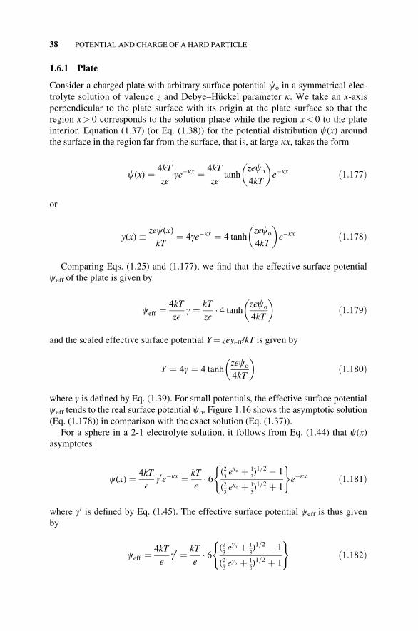
1.6.1 Plate

Consider a charged plate with arbitrary surface potential co in a symmetrical elec-

trolyte solution of valence z and Debye–Huckel parameter k. We take an x-axisperpendicular to the plate surface with its origin at the plate surface so that the

region x> 0 corresponds to the solution phase while the region x< 0 to the plate

interior. Equation (1.37) (or Eq. (1.38)) for the potential distribution c(x) aroundthe surface in the region far from the surface, that is, at large kx, takes the form

c(x) ¼ 4kT

zege�kx ¼ 4kT

zetanh

zeco

4kT

� �e�kx ð1:177Þ

or

y(x) � zec(x)kT

¼ 4ge�kx ¼ 4 tanhzeco

4kT

� �e�kx ð1:178Þ

Comparing Eqs. (1.25) and (1.177), we find that the effective surface potential

ceff of the plate is given by

ceff ¼4kT

zeg ¼ kT

ze 4 tanh zeco

4kT

� �ð1:179Þ

and the scaled effective surface potential Y¼ zeyeff/kT is given by

Y ¼ 4g ¼ 4 tanhzeco

4kT

� �ð1:180Þ

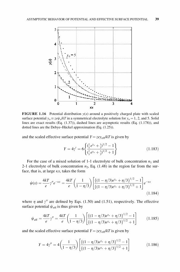
where g is defined by Eq. (1.39). For small potentials, the effective surface potential

ceff tends to the real surface potential co. Figure 1.16 shows the asymptotic solution

(Eq. (1.178)) in comparison with the exact solution (Eq. (1.37)).

For a sphere in a 2-1 electrolyte solution, it follows from Eq. (1.44) that c(x)asymptotes

c(x) ¼ 4kT

eg0e�kx ¼ kT

e 6 (2

3eyo þ 1

3)1=2 � 1

(23eyo þ 1

3)1=2 þ 1

( )e�kx ð1:181Þ

where g0 is defined by Eq. (1.45). The effective surface potential ceff is thus given

by

ceff ¼4kT

eg0 ¼ kT

e 6 (2

3eyo þ 1

3)1=2 � 1

(23eyo þ 1

3)1=2 þ 1

( )ð1:182Þ



Y ¼ 4g0 ¼ 6(23eyo þ 1

3)1=2 � 1

(23eyo þ 1

3)1=2 þ 1

( )ð1:183Þ

For the case of a mixed solution of 1-1 electrolyte of bulk concentration n1 and2-1 electrolyte of bulk concentration n2, Eq. (1.48) in the region far from the sur-

face, that is, at large kx, takes the form

c(x) ¼ 4kT

eg00e�kx ¼ 4kT

e

1

1� Z=3

� � f(1� Z=3)eyo þ Z=3g1=2 � 1

f(1� Z=3)eyo þ Z=3g1=2 þ 1

" #e�kx

ð1:184Þwhere Z and g00 are defined by Eqs. (1.50) and (1.51), respectively. The effective

surface potential ceff is thus given by

ceff ¼4kT

eg00 ¼ 4kT

e

1

1� Z=3

� � f(1� Z=3)eyo þ Z=3g1=2 � 1

f(1� Z=3)eyo þ Z=3g1=2 þ 1

" #ð1:185Þ


Y ¼ 4g00 ¼ 41

1� Z=3

� � f(1� Z=3)eyo þ Z=3g1=2 � 1

f(1� Z=3)eyo þ Z=3g1=2 þ 1

" #ð1:186Þ

FIGURE 1.16 Potential distribution y(x) around a positively charged plate with scaled

surface potential yo� zeco/kT in a symmetrical electrolyte solution for yo¼ 1, 2, and 5. Solid

lines are exact results (Eq. (1.37)), dashed lines are asymptotic results (Eq. (1.178)), and

dotted lines are the Debye–Huckel approximation (Eq. (1.25)).


We obtain the scaled effective surface potential Y for a plate having a surface

potential co (or scaled surface potential yo) immersed in a solution of general elec-

trolytes [9]. Integration of the Poisson–Boltzmann equation for the electric potential

c(x) is given by Eq. (1.65), namely,

kx ¼Z yo

y

dy

f (y)ð1:187Þ

where y¼ ec/kT and f(x) is defined by Eq. (1.56). Equation (1.187) can be

rewritten as

kx ¼Z yo

y

1

f (y)� 1

y

dyþ

Z yo

y

1

ydy

¼Z yo

y

1

f (y)� 1

y

dyþ ln yoj � ln yjjj

ð1:188Þ

Note here that the asymptotic form y(x) must be

y(x) ¼ constant exp(� kx) ð1:189Þor

kx ¼ constant� ln yjj ð1:190ÞTherefore, the integral term of (1.188) must become independent of y at large x.

Since y tends to zero in the limit of large x, the lower limit of the integration may be

replaced by zero. We thus find that the asymptotic form y(x) satisfies

kx ¼Z yo

0

1

f (y)� 1

y

dyþ ln yoj � ln yjjj ð1:191Þ

It can be shown that the asymptotic form of y(x) satisfies

y(x) ¼ Ye�kx ð1:192Þ

with

Y ¼ yo exp

Z yo

0

1

f (y)� 1

y

dy

� �ð1:193Þ

Equation (1.193) is the required expression for the scaled effective surface potential

(or the asymptotic constant) Y. Wilemski [11] has derived an expression for Y (Eq.

(15) with Eq. (12) in his paper [11]), which can be shown to be equivalent to Eq.

(1.193). For a planar surface having scaled surface potentials yo in a z-z symmetrical

electrolyte solution, Eq. (1.193) reproduces Eq. (1.180). Similarly, for the case of a


planar surface having a scaled surface potential yo in a 2-1 electrolyte solution, Eq.

(1.193) reproduces Eq. (1.183), while for the case of a mixed solution of 1-1 electro-

lyte of concentration n1 and 2-1 electrolyte of concentration n2, it gives Eq. (1.186).

1.6.2 Sphere

The asymptotic expression for the potential of a spherical particle of radius a in a

symmetrical electrolyte solution of valence z and Debye–Huckel parameter k at a

large distance r from the center of the sphere may be expressed as

c(r) ¼ ceff

a


y(r) ¼ ze

kTc(r) ¼ Y

a


where r is the radial distance measured from the sphere center, ceff is the effec-

tive surface potential, and Y¼ zeceff/kT is the scaled effective surface potential of a

sphere. From Eq. (1.122) we obtain

ceff ¼kT

ze 8 tanh(yo=4)

1þ f1� ((2kaþ 1)=(kaþ 1)2)tanh2(yo=4)g1=2ð1:196Þ

or

Y ¼ 8 tanh(yo=4)

1þ f1� ((2kaþ 1)=(kaþ 1)2)tanh2(yo=4)g1=2ð1:197Þ

It can be shown that ceff reduces to the real surface potential co in the low-po-

tential limit.

We obtain an approximate expression for the scaled effective surface potential Yfor a sphere of radius a having a surface potential co (or scaled surface potential

yo¼ eyo/kT) immersed in a solution of general electrolytes [9]. The Poisson–

Boltzmann equation for the scaled electric potential y(r)¼ ec/kT is approximately

given by Eq. (1.137), namely,

�ln s ¼Z yo

y

dy

F(y)ð1:198Þ

with

s ¼ a

rexp(� k(r � a)) ð1:199Þ

where F(y) is defined by Eq. (1.133). It can be shown that the scaled effective sur-

face potential Y¼ eceff/kT is given by

Y ¼ yoexp

Z yo

0

1

F(y)� 1

y

dy

� �ð1:200Þ


Equation (1.200) is the required expression for the scaled effective surface po-

tential (or the asymptotic constant) Y and reproduces Eq. (1.197) for a sphere of

radius a having a surface potential co in a symmetrical electrolyte solution of va-

lence z. The relative error of Eq. (1.200) is less than 1% for ka� 1.

1.6.3 Cylinder

The effective surface potential ceff or scaled effective surface potential Y¼ zeceff/

kT of a cylinder in a symmetrical electrolyte solution of valence z can be obtained

from the asymptotic form of the potential around the cylinder, which in turn is de-

rived from Eq. (1.157) as [7]

y(r) ¼ Yc ð1:201Þ

with

c ¼ K0(kr)K0(ka)

ð1:202Þ

and

Y ¼ 8 tanh(yo=4)

1þ f1� (1� b2)tanh2(yo=4)g1=2

ð1:203Þ

where r is the distance from the axis of the cylinder and

b ¼ K0(ka)K1(ka)

ð1:204Þ

We obtain an approximate expression for the scaled effective surface potential Yfor a cylinder of radius a having a surface potential ceff (or scaled surface potential

Y¼ eceff/kT) immersed in a solution of general electrolytes . The Poisson–

Boltzmann equation for the scaled electric potential y(r)¼ ec/kT is approximately

given by Eq. (1.176), namely,

�ln c ¼Z yo

y

dy

F(y)ð1:205Þ

where F(y) is defined by Eq. (1.168). It can be shown that the scaled effective sur-

face potential Y¼ eceff/kT is given by

Y ¼ yoexp

Z yo

0

1

F(y)� 1

y

dy

� �ð1:206Þ

Equation (1.206) reproduces Eq. (1.203) for a cylinder in a symmetrical electrolyte

solution of valence z. The relative error of Eq. (1.206) is less than 1% for ka� 1.


1.7 NEARLY SPHERICAL PARTICLE

So far we have treated uniformly charged planar, spherical, or cylindrical particles.

For general cases other than the above examples, it is not easy to solve analytically

the Poisson–Boltzmann equation (1.5). In the following, we give an example in

which one can derive approximate solutions.

We give below a simple method to derive an approximate solution to the linear-

ized Poisson–Boltzmann equation (1.9) for the potential distribution c(r) around a

nearly spherical spheroidal particle immersed in an electrolyte solution [12]. This

method is based on Maxwell’s method [13] to derive an approximate solution to the

Laplace equation for the potential distribution around a nearly spherical particle.

Consider first a prolate spheroid with a constant uniform surface potential co in

an electrolyte solution (Fig. 1.17a). The potential c is assumed to be low enough to

obey the linearized Poisson–Boltzmann equation (1.9). We choose the z-axis as theaxis of symmetry and the center of the prolate as the origin. Let a and b be the major

and minor axes of the prolate, respectively. The equation for the surface of the pro-

late is then given by

x2 þ y2

b2þ z2

a2¼ 1 ð1:207Þ

We introduce the spherical polar coordinate (r, �, �), that is, r2¼ x2þ y2þ z2 andz¼ r cos �, and the eccentricity of the prolate

ep ¼ffiffiffiffiffiffiffiffiffiffiffiffiffiffiffiffiffiffiffiffiffi1� (b=a)2

qð1:208Þ

Then, when the spheroid is nearly spherical (i.e., for low ep), Eq. (1.207) be-comes

r ¼ a 1� e2p2sin2 �

!¼ a 1þ e2p

3

1

2(3 cos2 �� 1)� 1

" #ð1:209Þ

FIGURE 1.17 Prolate spheroid (a) and oblate spheroid (b). a and b are the major and

minor semiaxes, respectively. The z-axis is the axis of symmetry.

NEARLY SPHERICAL PARTICLE 43

which is an approximate equation for the surface of the prolate with low eccentric-

ity ep (which is correct to order e2p).

The solution to Eq. (1.9) must satisfy the boundary conditions that c tends to zero

as r!1 and c¼co at the prolate surface (given by Eq. (1.209)). We thus obtain

c(r; �) ¼ co

a

re�k(r�a) � co

(1þ ka)3

e2pa

re�k(r�a) � k2(kr)

4k2(ka)(3 cos2 �� 1)

ð1:210Þ

where kn(z) is the modified spherical Bessel function of the second kind of order n.We can also obtain the surface charge density s(�) from Eq. (1.210), namely,

s(�) ¼ �ereo@c@n

¼ �ereo cos a@c@r

at r ¼ a 1þ e2p3

1

2(3 cos2 �� 1)� 1

" #

ð1:211Þwhere a is the angle between n and r. It can be shown that cos a ¼ 1þ O(e4p). Thenwe find from Eqs. (1.210) and (1.211) that

s(�)ereokco

¼ 1þ 1

kaþ e2p3ka

1��

2þ 2kaþ (ka)2

�(1þ ka)f9þ 9kaþ 4(ka)2 þ (ka)3g

2f3þ 3kaþ (ka)2g (3 cos2 �� 1)

� ð1:212Þ

Figure 1.18 shows equipotential lines (contours) around a prolate spheroid on the

z–x plane at y¼ 0, calculated from Eq. (1.210) at ka¼ 1.5 and kb¼ 1.

FIGURE 1.18 Equipotential lines (contours) around a prolate spheroid on the z–x plane aty¼ 0. Calculated from Eq. (1.210) at ka¼ 1.5 and kb¼ 1 (arbitrary size).


We next consider the case of an oblate spheroid with constant surface potential

co (Fig. 1.17b). The surface of the oblate is given by

x2 þ y2

a2þ z2

b2¼ 1 ð1:213Þ

where the z-axis is again the axis of symmetry, a and b are the major and minor

semiaxes, respectively. Equation (1.213) can be approximated by

r ¼ a 1þ e2o2sin2 �

� �¼ a 1� e2o

3

1

2(3 cos2 �� 1)� 1

� �ð1:214Þ

where the eccentricity eo of the oblate is given by

eo ¼ffiffiffiffiffiffiffiffiffiffiffiffiffiffiffiffiffiffiffiffiffi(a=b)2 � 1

qð1:215Þ

After carrying out the same procedure as employed for the case of the prolate

spheroid, we find that c(r, �) and the s–co relationship, both correct to order e2o, are

given by

c(r; �) ¼ co

b

re�k(r�b) � co

(1þ kb)3

e2ob

re�k(r�b) � k2(kr)

4k2(kb)(3 cos2 �� 1)

ð1:216Þ

s(�)ereokco

¼ 1þ 1

kb� e2o3kb

1�½ 2þ 2kbþ (kb)2�

�(1þ kb)f9þ 9kbþ 4(kb)2 þ (kb)3g

2f3þ 3kbþ (kb)2g (3 cos2 �� 1)

� ð1:217Þ

which can also be obtained directly from Eqs. (1.210) and (1.212) by interchanging

a$ b and replacing e2p by �e2o.The last term on the right-hand side of Eqs. (1.210), (1.212), (1.216), and (1.217)

corresponds to the deviation of the particle shape from a sphere.

REFERENCES

1. B. V. Derjaguin and L. Landau, Acta Physicochim. 14 (1941) 633.

2. E. J. W. Verwey and J. Th. G. Overbeek, Theory of the Stability of Lyophobic Colloids,Elsevier, Amsterdam, 1948.

3. H. Ohshima and K. Furusawa (Eds.), Electrical Phenomena at Interfaces: Fundamentals,Measurements, and Applications, 2nd edition, revised and expanded, Dekker, New York,

1998.

4. H. Ohshima, Theory of Colloid and Interfacial Electric Phenomena, Elsevier/Academic

Press, Amsterdam, 2006.

REFERENCES 45

5. A. L. Loeb, J. Th. G. Overbeek, and P. H. Wiersema, The Electrical Double LayerAround a Spherical Colloid Particle, MIT Press, Cambridge, MA, 1961.

6. L. R. White, J. Chem. Soc., Faraday Trans. 2 73 (1977) 577.

7. H. Ohshima, T. W. Healy, and L. R. White, J. Colloid Interface Sci. 90 (1982) 17.

8. H. Ohshima, J. Colloid Interface Sci. 171 (1995) 525,

9. H. Ohshima, J. Colloid Interface Sci. 174 (1995) 45.

10. H. Ohshima, J. Colloid Interface Sci. 200 (1998) 291.

11. G. Wilemski, J. Colloid Interface Sci. 88 (1982) 111.

12. H. Ohshima, Colloids Surf. A: Physicochem. Eng. Aspects 169 (2000) 13.

13. J. C. Maxwell, A Treatise on Electricity and Magnetism, Vol. 1, Dover, New York, 1954

p. 220.


Documents

Biophysical Chemistry of Biointerfaces (Ohshima/Biophysical Chemistry of Biointerfaces) || Potential and Charge of a Hard Particle