PART IVOther Topics

28 Membrane Potential andDonnan Potential

28.1 INTRODUCTION

When two electrolyte solutions at different concentrations are separated by an ion-

-permeable membrane, a potential difference is generally established between the

two solutions. This potential difference, known as membrane potential, plays an

important role in electrochemical phenomena observed in various biomembrane

systems. In the stationary state, the membrane potential arises from both the diffu-

sion potential [1,2] and the membrane boundary potential [3–6]. To calculate the

membrane potential, one must simultaneously solve the Nernst–Planck equation

and the Poisson equation. Analytic formulas for the membrane potential can be de-

rived only if the electric field within the membrane is assumed to be constant [1,2].

In this chapter, we remove this constant field assumption and numerically solve the

above-mentioned nonlinear equations to calculate the membrane potential [7].

28.2 MEMBRANE POTENTIAL AND DONNAN POTENTIAL

Imagine the stationary flow of electrolyte ions across a membrane separating solu-

tions I and II that contain uni–uni symmetrical electrolyte at different concentrations

nI and nII, respectively. We employ a membrane model [7] in which each side of the

membrane core of thickness dc is covered by a surface charge layer of thickness ds.In this layer, membrane-fixed negative charges are assumed to be distributed at a

uniform density N. We take the x-axis perpendicular to the membrane with its origin

at the boundary between the left surface charge layer and the membrane core

(Fig. 28.1). The potential in the bulk phase of solution II is set equal to zero.

The potential in bulk solution I is thus equal to the membrane potential, which

we denote by Em. First, consider the regions x< 0 and x> dc. We assume that the

distribution of electrolyte ions in the surface charge layer and in solutions I and II is

scarcely affected by ionic flows so that it is in practice at thermodynamic equili-

Biophysical Chemistry of Biointerfaces By Hiroyuki OhshimaCopyright# 2010 by John Wiley & Sons, Inc.

535

brium. Accordingly, the potential c(x) in these regions is given by the Poisson–

Boltzmann equations, namely,

d2cdx2

¼ 2enIereo

sinheðc� EmÞ

kT

� �; x < �ds ð28:1Þ

d2cdx2

¼ 2enIereo

sinheðc� EmÞ

kT

� �þ eN

ereo; � ds < x < 0 ð28:2Þ

d2cdx2

¼ 2enIIereo

sinheckT

� �þ eN

ereo; dc þ ds < x < dc ð28:3Þ

d2cdx2

¼ 2enIIereo

sinheckT

� �; x > dc þ ds ð28:4Þ

where er is the relative permittivity of solutions I and II. Next, consider the region

0< x< dc (i.e., the membrane core). We regard this region as a different phase from

the surrounding solution phase and introduce the ionic partition coefficients

between the membrane core and the solution phase. We denote by b+ and b�,respectively, the partition coefficients for cations and anions. The electric potential

c(x) in this region is given by the following Poisson equation:

d2cdx2

¼ e

e0reonþðxÞ � n�ðxÞf g; 0 < x < dc ð28:5Þ

FIGURE 28.1 Model for a charged membrane. The membrane core (of thickness dc) iscovered by a surface charge layer (of thickness ds). The membrane-fixed charges are assumed

to be negative and are encircled.

536 MEMBRANE POTENTIAL AND DONNAN POTENTIAL

where nþ(x) and n�(x) are the respective concentrations of cations and anions at

position x (0< x< dc) and e0r is the relative permittivity of the membrane core. The

flow of cations, denoted by Jþ, can be expressed as the product of the number den-

sity nþ(x) and velocity vþ of cations. Similarly, the flow J� of anions can be

expressed as the product of the number density n�(x) and velocity v� of anions.

That is,

J� ¼ n�v� ð28:6Þ

The ionic velocities v� are given by

v� ¼ � 1

l�

dm�dx

ð28:7Þ

Here, l� are the ionic drag coefficients of cations and anions, respectively, and

m� are the electrochemical potentials of cations and anions, respectively, which are

m� ¼ mo� þ kT lnn�ðxÞ � zecðxÞ ð28:8Þ

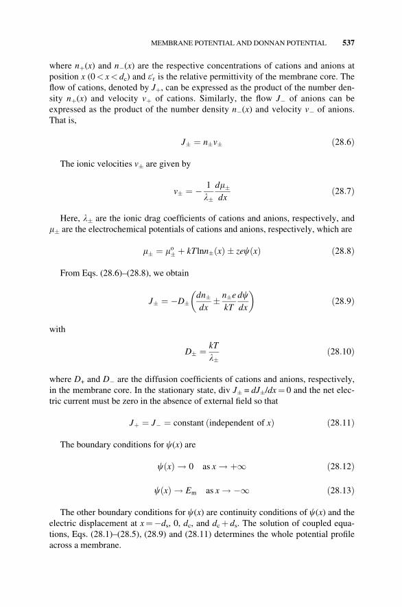
From Eqs. (28.6)–(28.8), we obtain

J� ¼ �D�dn�dx

� n�ekT

dcdx

� �ð28:9Þ

with

D� ¼ kT

l�ð28:10Þ

where D+ and D� are the diffusion coefficients of cations and anions, respectively,

in the membrane core. In the stationary state, div J�=dJ�/dx¼ 0 and the net elec-

tric current must be zero in the absence of external field so that

Jþ ¼ J� ¼ constant ðindependent of xÞ ð28:11Þ

The boundary conditions for c(x) are

cðxÞ ! 0 as x ! þ1 ð28:12Þ

cðxÞ ! Em as x ! �1 ð28:13Þ

The other boundary conditions for c(x) are continuity conditions of c(x) and the

electric displacement at x¼�ds, 0, dc, and dcþ ds. The solution of coupled equa-

tions, Eqs. (28.1)–(28.5), (28.9) and (28.11) determines the whole potential profile

across a membrane.

MEMBRANE POTENTIAL AND DONNAN POTENTIAL 537

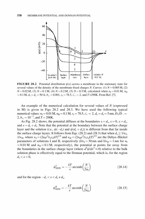
An example of the numerical calculation for several values of N (expressed

in M) is given in Figs 28.2 and 28.3. We have used the following typical

numerical values: nI¼ 0.01M, nII¼ 0.1M, er¼ 78.5, e0r ¼ 2, dc¼ ds¼ 5nm,D+/D�¼2, b�¼ 10�3, and T¼ 298K.

As Fig. 28.2 shows, the potential diffuses at the boundaries x¼ ds, x¼ 0, x¼ dc,and x¼ dcþ ds. Note that the potential at the boundary between the surface charge

layer and the solution (i.e., c(�ds) and c(dcþ ds)) is different from that far inside

the surface charge layers. It follows from Eqs. (28.2) and (28.3) that when ds� 1/kI,1/kII, where kI¼ (2nIe

2/ereokT)1/2 and kII¼ (2nIIe

2/ereokT)1/2 are the Debye–Huckel

parameters of solutions I and II, respectively (l/kI¼ 30 nm and l/kII¼ 1 nm for nI¼ 0.01M and nII¼ 0.1M, respectively), the potential at points far away from

the boundaries in the surface charge layer (where d2c/dx2� 0) relative to the bulk

solution phase is effectively equal to the Donnan potential, which is, for the region

ds< x< 0,

cIDON ¼ � kT

earcsinh

N

2nI

� �ð28:14Þ

and for the region �dc< x< dc + ds,

cIIDON ¼ � kT

earcsinh

N

2nII

� �ð28:15Þ

FIGURE 28.2 Potential distribution c(x) across a membrane in the stationary state for

several values of the density of the membrane-fixed charges N. Curves: (1) N¼ 0.005M, (2)

N¼ 0.02M, (3) N¼ 0.1M, (4) N¼ 0.2M, (5) N¼ 0.5M, calculated when nI¼ 0.01M, nII¼ 0.1M, ds¼ dc¼ 50A, b�¼ 0.001, er¼ 78.5, e

0r ¼ 2, and T =298K. From Ref. [7].

538 MEMBRANE POTENTIAL AND DONNAN POTENTIAL

In this case, by integrating Eqs. (28.1)–(28.4) once and using the appropriate

boundary conditions, we have

cð�dsÞ ¼ cIDON � kT

etanh

ecIDON

2kT

� �þ Em ð28:16Þ

cðdc þ dsÞ ¼ cIIDON � kT

etanh

ecIIDON

2kT

� �ð28:17Þ

which relate the membrane surface potentials c(�ds) and c(dc + ds) to the Donnan

potentials cIDON and cI

DON. When the potential far inside the surface charge layer is

effectively equal to the Donnan potential, the membrane potential can be expressed as

Em ¼ fcð0Þ � cðdcÞg þ fcIIDON � cI

DONg þ ½fcIDON þ Em � cð0Þg

�fcIIDON � cðdcÞg� ð28:18Þ

where the first term enclosed by brackets on the right-hand side corresponds to

the diffusion potential, the second to the contribution from the Donnan potentials in

the surface charge layers, and the third to that from deviation in the boundary poten-

tials at x¼ 0 and x¼ dc due to the ionic flows. The contribution from the third term

is normally very small so that the diffusion potential E can practically be regarded as

arising from the diffusion potential and the Donnan potential. Note that the

FIGURE 28.3 Membrane potential Em, contributions from the diffusion potential Ed

and the Donnan potential difference DcDON ¼ cIIDON � cI

DON as functions of the density of

membrane-fixed charges N. The values of the parameters used in the calculation are the same

as those in Fig. 28.2. The dashed line is the approximate result for Em (Eq. (28.21)). As

N!1, Em tends to the Nernst potential for cations (59mV in the present case). From Ref. [7].

MEMBRANE POTENTIAL AND DONNAN POTENTIAL 539

Donnan potentials (Eqs. (28.14) and (28.15)) are independent of the surface layer

thickness ds and therefore the membrane potential depends little on ds, provided that

ds� 1/kI, 1/kII.Figure 28.2 (in which the potential far inside the surface layer is almost equal to

the Donnan potential) shows how the contributions from the diffusion potential and

from the Donnan potential change with density N of the membrane-fixed charges.

For very low N, the potential in the surface charge layer differs little from that in

the bulk solution phase (the Donnan potential itself is very small) and the mem-

brane potential is mostly due to the potential gradient in the membrane core. In

other words, the membrane potential is almost equal to the diffusion potential. As

N is increased, however, the potential gradient in the membrane core becomes

small, which means that the contribution from the diffusion potential decreases. In-

stead, the potential difference between the surface charge layer and the surrounding

solution becomes appreciable and the membrane potential for very large N is deter-

mined almost solely by the potential difference in each surface charge layer. As

stated before, the potential difference is in practice equal to the Donnan potential in

each surface charge layer if ds� 1/kI, 1/kII so that the membrane potential Em for

large N is expressed as

Em ¼ cIIDON � cI

DON

¼ kT

eln

ðN=2nIÞ þ fðN=2nIÞ2 þ 1g1=2

ðN=2nIIÞ þ fðN=2nIIÞ2 þ 1g1=2" #

þ cIIs � cI

s

ð28:19Þ

To illustrate more clearly the above-mentioned N dependence, we have dis-

played in Fig. 28.3 the contributions from the diffusion and Donnan potentials to

the membrane potential as a function of N.The decrease of the contribution from the diffusion potential with increasing N

can be explained as follows. For large N, that is, for the case where the surface

layers are highly negatively charged, coions (i.e., anions) are repelled by the mem-

brane so that the membrane is in practice impermeable to coions and their flow

within the membrane, J�, decreases. Since the net electric current must be zero (Jþ� J�¼ 0), the flow of counterions (i.e., cations), Jþ, must decrease to the same

extent as J�. That is, all ionic flows decrease, resulting in a smaller diffusion poten-

tial. In the limit of N!1, the membrane becomes fully impermeable to anions and

an equilibrium is reached with respect to cations so that the membrane potential

tends to the Nernst potential for cations, namely,

Em ! kT

eln

nIInI

� �ð28:20Þ

which is obtained by taking the limit N!1 in Eq. (28.19). In this limit, the mem-

brane behaves like a semipermeable membrane (permeable to cations only). Note

that Eq. (28.20) also holds when b�! 0, irrespective of the value of N.

540 MEMBRANE POTENTIAL AND DONNAN POTENTIAL

As shown in Fig. 28.2, the potential gradient in the membrane core is slightly

concave (see curve 3, in particular). However, deviation from linearity is seen to be

small in Fig. 28.2. This means that the usual assumption of constant field within the

membrane is not a bad approximation. If we employ this approximation, Eq. (28.9)

can easily be integrated in the following two limiting cases. When ds� 1/kI, 1/kII,in which case the potential far inside the membrane surface layer is in practice the

Donnan potential, the constant field assumption yields [3]

Em ¼ kT

eln

PþnII expð�ecIIDON=kTÞ þ P�nI expðecI

DON=kTÞPþnI expð�ecI

DON=kTÞ þ P�nII expðecIIDON=kTÞ

" #þ cII

DON � cIDON

ð28:21Þ

with

P� ¼ b�D�=dc ð28:22Þ

where Pþ and P� are the permeabilities of cations and anions, respectively. The

approximate result calculated from Eq. (28.21) is plotted in Fig. 28.3 in comparison

with the exact numerical results. A good agreement is obtained: the relative error is

less than a few percent. On the other hand, in the limit ds! 0 with Nds kept con-stant, we can then obtain the following formula [5,6]:

Em ¼ kT

eln

PþnII expð�ecIIs =kTÞ þ P�nI expðecI

s=kTÞPþnI expð�ecI

s=kTÞ þ P�nII expðecIIs =kTÞ

" #þ cII

s � cIs ð28:23Þ

where

cIs ¼

2kT

earcsinh

s

ð8nIereokTÞ1=2" #

ð28:24Þ

cIIs ¼ 2kT

earcsinh

s

ð8nIIereokTÞ1=2" #

ð28:25Þ

Equations (28.24) and (28.25) are the Gouy–Chapman double-layer potential of

the membrane surface with a surface charge density s¼�eNds.

REFERENCES

1. D. E. Goldman, J. Gen. Physiol. 27 (1943) 37.

2. A. L. Hodgkin and B. G. Katz, J. Physiol. 108 (1949) 37.

REFERENCES 541

3. M. J. Polissar, in: F. H. Johnson, H. Eyring, and M. J. Polissar (Eds.), Kinetic Basis ofMolecular Biology, Wiley, New York, 1954, p. 515.

4. S. Ohki, in: J. F. Danielli (Ed.), Progress in Surface and Membrane Science, Vol. 10,Academic Press, New York, 1976, p. 117.

5. S. Ohki, Phys. Lett. 75A (1979) 149.

6. S. Ohki, Physiol. Chem. Phys. 13 (1981) 195.

7. H. Ohshima and T. Kondo, Biophys. Chem. 29 (1988) 277.

542 MEMBRANE POTENTIAL AND DONNAN POTENTIAL