Biophysical Chemistry of Biointerfaces (Ohshima/Biophysical Chemistry of Biointerfaces) || Effective Viscosity of a Suspension of Soft Particles

27 Effective Viscosityof a Suspension ofSoft Particles

27.1 INTRODUCTION

The effective viscosity Zs of a dilute suspension of uncharged colloidal particles in

a liquid is greater than the viscosity Z of the original liquid. Einstein [1] derived the

following expression for Zs:

Zs ¼ Z 1þ 5

2�

� �ð27:1Þ

where � is the particle volume fraction.

For concentrated suspensions, hydrodynamic interactions among particles must

be considered. The hydrodynamic interactions between spherical particles can be

taken into account by means of a cell model, which assumes that each sphere of

radius a is surrounded by a virtual shell of outer radius b and the particle volume

fraction � is given by

� ¼ ða=bÞ3 ð27:2ÞSimha [2] derived the following equation for the effective viscosity Zs of a con-

centrated suspension of uncharged particles of volume fraction �:

Zs ¼ Z 1þ 5

2�Sð�Þ

� �ð27:3Þ

with

Sð�Þ ¼ 4ð1� �7=3Þ4ð1þ �10=3Þ � 25�ð1þ �4=3Þ þ 42�5=3

¼ 4ð1� �7=3Þ4ð1� �5=3Þ2 � 25�ð1� �2=3Þ2

ð27:4Þ

Biophysical Chemistry of Biointerfaces By Hiroyuki OhshimaCopyright# 2010 by John Wiley & Sons, Inc.

515

where S(�) is called Simha’s function. As �! 0, S(�) tends to 1 so that Eq. (27.3)

reduces back to Einstein’s equation (27.1).

If the liquid contains an electrolyte and the particles are charged, then the effec-

tive viscosity Zs is further increased. This phenomenon is called the primary electro-

viscous effect [3–18] and the effective viscosity Zs can be expressed as

Zs ¼ Z 1þ 5

2ð1þ pÞ�

� �ð27:5Þ

where p is the primary electroviscous coefficient. The standard theory for this effect

and the governing electrokinetic equations as well as their numerical solutions were

given by Watterson and White [9]. Ohshima [17,18] derived an approximate ana-

lytic expression for p in a dilute suspension of spherical particles with arbitrary zetapotentials and large ka (where k is the Debye–Huckel parameter and a is the parti-

cle radius). The standard theory of the primary electroviscous effect has been

extended to cover the case of concentrated suspensions of charged spherical

particles with thin electrical double layers under the condition of nonoverlapping

electrical double layers of adjacent particles by Ruiz-Reina et al. [19] and

Rubio-Hern�andez et al. [20]. Ohshima [21] has recently derived an approximate

analytic expression for p in a moderately concentrated suspension of spherical

particles with arbitrary zeta potential and large ka.The effective viscosity of a suspension of particles of types other than rigid

particles has also been theoretically investigated. Taylor [22] proposed a theory of

the electroviscous effect in a suspension of uncharged liquid drops. This theory

has been extended to the case of charged liquid drops by Ohshima [17]. Natraj

and Chen [23] developed a theory for charged porous spheres, and Allison et al.

[24] and Allison and Xin [25] discussed the case of polyelectrolyte-coated

particles.

In this chapter, we first present a theory of the primary electroviscous effect in

a dilute suspension of soft particles, that is, particles covered with an ion-penetra-

ble surface layer of charged or uncharged polymers. We derive expressions for the

effective viscosity and the primary electroviscous coefficient of a dilute suspen-

sion of soft particles [26]. We then derive an expression for the effective viscosity

of uncharged porous spheres (i.e., spherical soft particles with no particle core)

[27].

27.2 BASIC EQUATIONS

Consider a dilute suspension of spherical soft particles in an electrolyte solution

of volume V in an applied shear field. We assume that the uncharged particle

core of radius a is coated with an ion-penetrable layer of polyelectrolytes of thick-

ness d. The polymer-coated particle has thus an inner radius a and an outer radius

b¼ aþ d. The origin of the spherical polar coordinate system (r, �, j) is held fixed

at the center of one particle. We consider the case where dissociated groups of

516 EFFECTIVE VISCOSITY OF A SUSPENSION OF SOFT PARTICLES

valence Z are distributed with a uniform density N in the polyelectrolyte layer so

that the density of the fixed charges rfix in the surface layer is given by rfix¼ ZeN,where e is the elementary electric charge. Let the electrolyte be composed of Mionic mobile species of valence zi, bulk concentration (number density) n1i , and

drag coefficient li (i¼ 1, 2, . . . ,M). The drag coefficient li of the ith ionic speciesis related to the limiting conductance L0

i of that ionic species by Eq. (21.9). We

adopt the model of Debye–Bueche, in which the polymer segments are regarded as

resistance centers distributed in the polyelectrolyte layer, exerting frictional forces

�gu on the liquid flowing in the polymer layer, where u is the liquid velocity rela-

tive to the particle and g is the frictional coefficient (Chapter 21). The main assump-

tions in our analysis are as follows: (i) The Reynolds numbers of the liquid flows

outside and inside the polyelectrolyte layer are small enough to ignore inertial terms

in the Navier–Stokes equations and the liquid can be regarded as incompressible.

(ii) The applied shear field is weak so that electrical double layer around the particle

is only slightly distorted. (iii) The slipping plane (at which the liquid velocity rela-

tive to the particle becomes zero) is located on the particle core surface. (iv) No

electrolyte ions can penetrate the particle core. (v) The polyelectrolyte layer is per-

meable to mobile charged species. (vi) The relative permittivity er takes the same

value both inside and outside the polyelectrolyte layer.

Imagine that a linear symmetric shear field u(0)(r) is applied to the system so that

the velocity u(r) at position r outside the particle core is given by the sum of u(0)(r)and a perturbation velocity. Thus, u(r) obeys the boundary condition

uðrÞ ! uð0ÞðrÞ as r ! 1 ð27:6Þ

where f(r) is a function of r (r ¼ jrj). We can express u(0)(r) as

uð0ÞðrÞ ¼ a � r ð27:7Þ

where a is a symmetric traceless tensor so that u(0)(r) becomes irrotational, namely,

r� uð0Þ ¼ 0 ð27:8Þ

Also we have from assumption (i) the following continuity equations:

r � uð0Þ ¼ 0 ð27:9Þ

r � u ¼ 0 ð27:10Þ

From symmetry considerations u(r) takes the form

uðrÞ ¼ uð0ÞðrÞ þ r �r� ½ða � rÞ f ðrÞ� ð27:11Þ

BASIC EQUATIONS 517

where f(r) is a function of r and the second term on the right-hand side corresponds

to the perturbation velocity. We introduce a function h(r), defined by

hðrÞ ¼ d

dr

1

r

df

dr

� �ð27:12Þ

then Eq. (27.11) can be rewritten as

uðrÞ ¼ uð0ÞðrÞ þ r � hðrÞr

r� uð0ÞðrÞ� �

¼ 1� dh

dr� 2h

r

� �uð0Þ þ 1

r2dh

dr� h

r

� �rðr � uð0ÞÞ

ð27:13Þ

where h(r) is a function of r only and we have used Eq. (27.8) (irrotational flow),

Eq. (27.9) (incompressible flow), and (r�Ï)u(0)¼ u(0) (linear flow). The basic equa-tions for the liquid flow u(r) and the velocity vi(r) of the ith ionic species are similar

to those for the electrophoresis problem. The boundary conditions for u and vi(r) atr¼ a and r¼ b are the same as those for the electrophoresis problem.

27.3 LINEARIZED EQUATIONS

For a weak shear field (assumption (ii)), as in the case of the electrophoresis

problem (Chapter 21), one may write

niðrÞ ¼ nð0Þi ðrÞ þ dniðrÞ ð27:14Þ

cðrÞ ¼ cð0ÞðrÞ þ dcðrÞ ð27:15Þ

miðrÞ ¼ mð0Þ þ dmiðrÞ ð27:16Þ

relðrÞ ¼ rð0Þel ðrÞ þ drelðrÞ ð27:17Þ

where the quantities with superscript (0) refer to those at equilibrium (i.e., in the

absence of the shear field), and dni(r), dc(r), dmi(r), and drel(r) are perturbation

quantities.

Symmetry considerations permit us to write

dmiðrÞ ¼ �zie�iðrÞr2

r � uð0ÞðrÞ ð27:18Þ


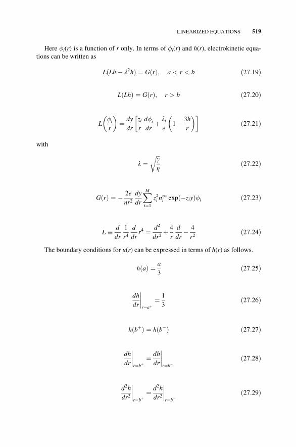
Here �i(r) is a function of r only. In terms of �i(r) and h(r), electrokinetic equa-tions can be written as

LðLh� l2hÞ ¼ GðrÞ; a < r < b ð27:19Þ

LðLhÞ ¼ GðrÞ; r > b ð27:20Þ

L�i

r

� �¼ dy

dr

zir

d�i

drþ li

e1� 3h

r

� �� ð27:21Þ

with

l ¼ffiffiffigZ

rð27:22Þ

GðrÞ ¼ � 2e

Zr2dy

dr

XMi¼1

z2i n1i expð�ziyÞ�i ð27:23Þ

L � d

dr

1

r4d

drr4 ¼ d2

dr2þ 4

r

d

dr� 4

r2ð27:24Þ

The boundary conditions for u(r) can be expressed in terms of h(r) as follows.

hðaÞ ¼ a

3ð27:25Þ

dh

dr

��r¼aþ

¼ 1

3ð27:26Þ

hðbþÞ ¼ hðb�Þ ð27:27Þ

dh

dr

��r¼bþ

¼ dh

dr

��r¼b�

ð27:28Þ

d2h

dr2

��r¼bþ

¼ d2h

dr2

��r¼b�

ð27:29Þ

LINEARIZED EQUATIONS 519

d3h

dr3

��r¼bþ

¼ d3h

dr3

��r¼b�

þ l2 1� dh

dr

��r¼b�

� 2hðb�Þb

� �ð27:30Þ

hðrÞ ! 0 as r ! 1 ð27:31Þ

hdh

dr! 0 as r ! 1 ð27:32Þ

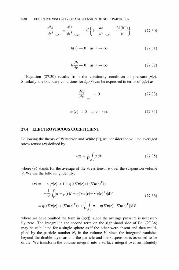
Equation (27.30) results from the continuity condition of pressure p(r).Similarly, the boundary conditions for dmi(r) can be expressed in terms of �i(r) as

d�i

dr

��r¼aþ

¼ 0 ð27:33Þ

�iðrÞ ! 0 as r ! 1 ð27:34Þ

27.4 ELECTROVISCOUS COEFFICIENT

Following the theory of Watterson and White [9], we consider the volume averaged

stress tensor kri defined by

hri ¼ 1

V

ZV

r dV ð27:35Þ

where kri stands for the average of the stress tensor s over the suspension volume

V. We use the following identity:

hri ¼ � < pðrÞ > I þ ZðhruðrÞiþhruðrÞTiÞ

þ 1

V

ZV

½rþ pðrÞI � ZðruðrÞþruðrÞTÞ�dV

¼ ZðhruðrÞiþhruðrÞTiÞ þ 1

V

ZV

½r� ZðruðrÞþruðrÞTÞ�dV

ð27:36Þ

where we have omitted the term in kp(r)i, since the average pressure is necessar-

ily zero. The integral in the second term on the right-hand side of Eq. (27.36)

may be calculated for a single sphere as if the other were absent and then multi-

plied by the particle number Np in the volume V, since the integrand vanishes

beyond the double layer around the particle and the suspension is assumed to be

dilute. We transform the volume integral into a surface integral over an infinitely


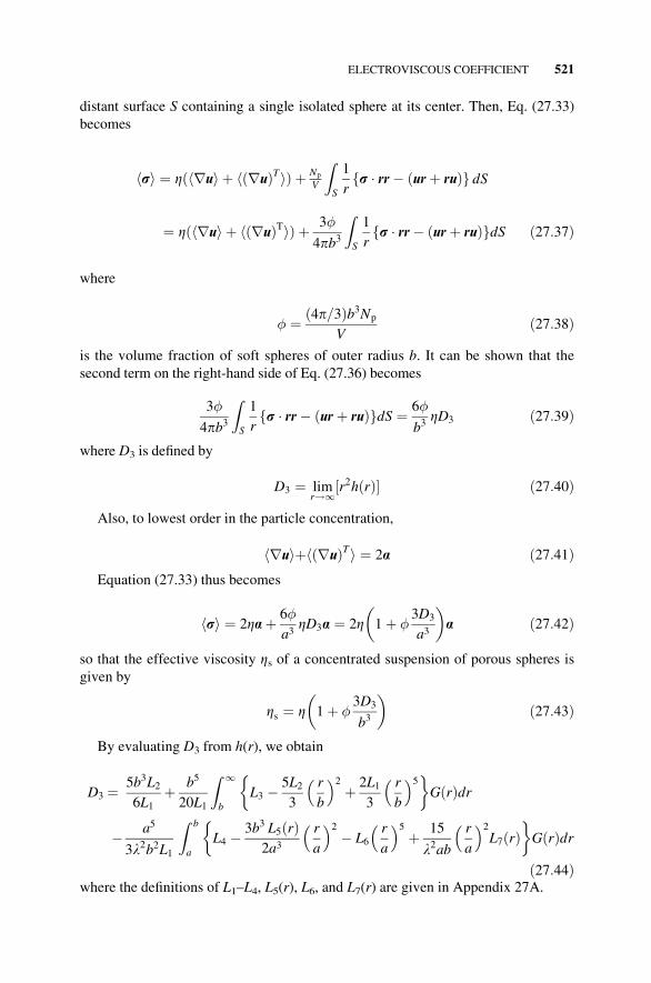
distant surface S containing a single isolated sphere at its center. Then, Eq. (27.33)

becomes

hri ¼ Zðhrui þ hðruÞTiÞ þ Np

V

ZS

1

rr � rr� ðurþ ruÞf g dS

¼ Zðhrui þ hðruÞTiÞ þ 3�

4pb3

ZS

1

rr � rr� ðurþ ruÞf gdS ð27:37Þ

where

� ¼ ð4p=3Þb3Np

Vð27:38Þ

is the volume fraction of soft spheres of outer radius b. It can be shown that the

second term on the right-hand side of Eq. (27.36) becomes

3�

4pb3

ZS

1

rr � rr� ðurþ ruÞf gdS ¼ 6�

b3ZD3 ð27:39Þ

where D3 is defined by

D3 ¼ limr!1½r

2hðrÞ� ð27:40ÞAlso, to lowest order in the particle concentration,

hruiþhðruÞTi ¼ 2a ð27:41ÞEquation (27.33) thus becomes

hri ¼ 2Zaþ 6�

a3ZD3a ¼ 2Z 1þ �

3D3

a3

� �a ð27:42Þ

so that the effective viscosity Zs of a concentrated suspension of porous spheres is

given by

Zs ¼ Z 1þ �3D3

b3

� �ð27:43Þ

By evaluating D3 from h(r), we obtain

D3 ¼ 5b3L26L1

þ b5

20L1

Z 1

b

L3 � 5L23

r

b

2þ 2L1

3

r

b

5� �GðrÞdr

� a5

3l2b2L1

Z b

a

L4 � 3b3 L5ðrÞ2a3

r

a

2� L6

r

a

5þ 15

l2ab

r

a

2L7ðrÞ

� �GðrÞdr

ð27:44Þwhere the definitions of L1–L4, L5(r), L6, and L7(r) are given in Appendix 27A.

ELECTROVISCOUS COEFFICIENT 521

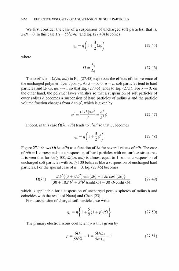
We first consider the case of a suspension of uncharged soft particles, that is,

ZeN¼ 0. In this case D3¼ 5b3L2/L1 and Eq. (27.40) becomes

Zs ¼ Z 1þ 5

2O�

� �ð27:45Þ

where

O ¼ L2L1

ð27:46Þ

The coefficient O(la, a/b) in Eq. (27.45) expresses the effects of the presence of

the uncharged polymer layer upon Zs. As l!1 or a! b, soft particles tend to hardparticles and O(la, a/b)! 1 so that Eq. (27.45) tends to Eq. (27.1). For l! 0, on

the other hand, the polymer layer vanishes so that a suspension of soft particles of

outer radius b becomes a suspension of hard particles of radius a and the particle

volume fraction changes from � to �0, which is given by

�0 ¼ ð4=3Þpa3V

¼ a3

b3� ð27:47Þ

Indeed, in this case O(la, a/b) tends to a3/b3 so that Zs becomes

Zs ¼ Z 1þ 5

2�0

� �ð27:48Þ

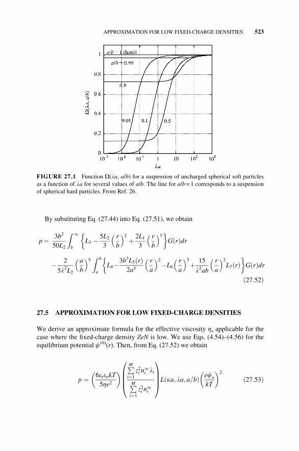
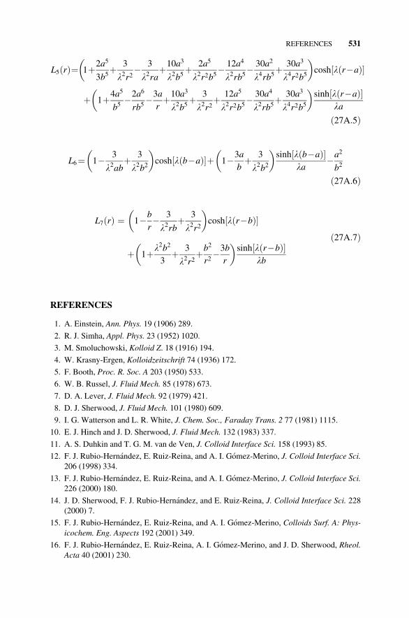
Figure 27.1 shows O(la, a/b) as a function of la for several values of a/b. The caseof a/b¼ 1 corresponds to a suspension of hard particles with no surface structures.

It is seen that for la� 100, O(la, a/b) is almost equal to 1 so that a suspension of

uncharged soft particles with la� 100 behaves like a suspension of uncharged hard

particles. For the special case of a¼ 0, Eq. (27.46) becomes

OðlbÞ ¼ l2b2fð3þ l2b2ÞsinhðlbÞ � 3 lb coshðlbÞgð30þ 10l2b2 þ l4b4ÞsinhðlbÞ � 30 lb coshðlbÞ ð27:49Þ

which is applicable for a suspension of uncharged porous spheres of radius b and

coincides with the result of Natraj and Chen [23].

For a suspension of charged soft particles, we write

Zs ¼ Z 1þ 5

2ð1þ pÞ�O

� �ð27:50Þ

The primary electroviscous coefficient p is thus given by

p ¼ 6D3

5b3O� 1 ¼ 6D3L1

5b3L2� 1 ð27:51Þ


By substituting Eq. (27.44) into Eq. (27.51), we obtain

p¼ 3b2

50L2

Z 1

b

L3 � 5L23

r

b

2þ 2L1

3

r

b

5� �GðrÞdr

� 2

5l2L2

a

b

5 Z b

a

L4�3b3L5ðrÞ2a3

r

a

2�L6

r

a

5þ 15

l2ab

r

a

2L7ðrÞ

� �GðrÞdr

ð27:52Þ

27.5 APPROXIMATION FOR LOW FIXED-CHARGE DENSITIES

We derive an approximate formula for the effective viscosity Zs applicable for the

case where the fixed-charge density ZeN is low. We use Eqs. (4.54)–(4.56) for the

equilibrium potential c(0)(r). Then, from Eq. (27.52) we obtain

p ¼ 6ereokT5Ze2

� � PMi¼1

z2i n1i li

PMi¼1

z2i n1i

0BBB@

1CCCALðka; la; a=bÞ eco

kT

� �2

ð27:53Þ

FIGURE 27.1 Function O(la, a/b) for a suspension of uncharged spherical soft particles

as a function of la for several values of a/b. The line for a/b= 1 corresponds to a suspension

of spherical hard particles. From Ref. 26.

APPROXIMATION FOR LOW FIXED-CHARGE DENSITIES 523

with

Lðka; la; a=bÞ ¼ k2b2

50L2

Z 1

b

L3 � 5L23

r

b

2þ 2L1

3

r

b

5� �1

co

dcð0Þ

dr

!HðrÞdr

� 2k2

15l2L2

a

b

5 Z b

a

L4 � 3b3L5ðrÞ2a3

r

a

2� L6

r

a

5�

þ 15

l2ab

r

a

2L7ðrÞ

�1

co

dcð0Þ

dr

!HðrÞdr ð27:54Þ

where H(r) is defined by

HðrÞ ¼ 1þ 2a5

3r5

� �Z 1

a

1

co

dcð0Þ

dx

!1� 3h

x

� �dx

�Z r

a

1

co

dcð0Þ

dx

!1� x5

r5

� �1� 3h

x

� �dx ð27:55Þ

One can calculate the primary electroviscous coefficient p for a suspension of

soft particles with low ZeN via Eq. (27.53).

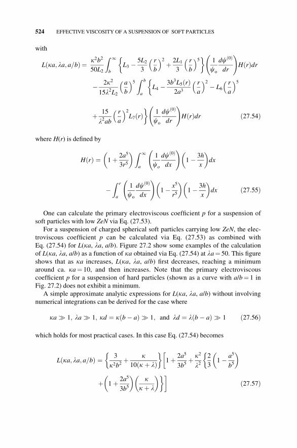
For a suspension of charged spherical soft particles carrying low ZeN, the elec-troviscous coefficient p can be calculated via Eq. (27.53) as combined with

Eq. (27.54) for L(ka, la, a/b). Figure 27.2 show some examples of the calculation

of L(ka, la, a/b) as a function of ka obtained via Eq. (27.54) at la¼ 50. This figure

shows that as ka increases, L(ka, la, a/b) first decreases, reaching a minimum

around ca. ka¼ 10, and then increases. Note that the primary electroviscous

coefficient p for a suspension of hard particles (shown as a curve with a/b¼ 1 in

Fig. 27.2) does not exhibit a minimum.

A simple approximate analytic expressions for L(ka, la, a/b) without involvingnumerical integrations can be derived for the case where

ka � 1; la � 1; kd ¼ kðb� aÞ � 1; and ld ¼ lðb� aÞ � 1 ð27:56Þ

which holds for most practical cases. In this case Eq. (27.54) becomes

Lðka; la; a=bÞ ¼ 3

k2b2þ k10ðkþ lÞ

� �1þ 2a5

3b5þ k2

l22

31� a5

b5

� ��

þ 1þ 2a5

3b5

� �k

kþ l

� ��ð27:57Þ


Consider several limiting cases for Eq. (27.57).

1. For the case of particles covered with a very thin polyelectrolyte layer (a� b),Eq. (27.54) becomes


k2b2þ k6ðkþ lÞ

� �1þ k2

l2k

kþ l

� �� ð27:58Þ

2. In the opposite limiting case of a very thick polyelectrolyte layer (a b).Eq. (27.57) tends to


k2b2þ k10ðkþ lÞ

� �1þ k2

l22

3þ k

kþ l

� �� ð27:59Þ

which is also applicable for a suspension of spherical polyelectrolyte with no

particle core (a¼ 0). The above two limiting cases, L(ka, la, a/b) does notdepend on the value of the inner radius a.

3. In the limit of l!1 (l� k), Eq. (27.57) tends to


k2b21þ 2a5

3b5

� �ð27:60Þ

FIGURE 27.2 Function L(ka, la, a/b) for a suspension of soft particles as a function of

ka for a/b¼ 0.5 and 0.9 at la¼ 50. The solid lines represent the results calculated via

Eq. (27.54) and the dotted lines approximate results calculated via Eq. (27.57). The curve for

a/b¼ 1 corresponds to a suspension of spherical hard particles. From Ref. 26.

APPROXIMATION FOR LOW FIXED-CHARGE DENSITIES 525

When a¼ b, Eq. (27.57) further becomes


k2b2ð27:61Þ

which agrees with the result for a suspension of hard spheres of radius b[16].

4. For k!1 (k� l)

Lðka; la; a=bÞ ¼ k2

6l2ð27:62Þ

Approximate results calculated via Eq. (27.57) are also shown as dotted lines in

Fig. 27.2. It is seen that ka� 100, the agreement with the exact result is excellent.

The presence of a minimum of L(ka, la, a/b) as a function of ka can be explained

qualitatively with the help of Eq. (27.57) as follows. That is, L(ka, la, a/b) is pro-portional to 1/k2 at small ka and to k2 at large ka, leading to the presence of a

minimum of L(ka, la, a/b). As is seen in Fig. 27.3, for the case of a suspension of

hard particles, the function L(ka) decreases as ka increases, exhibiting no mini-

mum. This is the most remarkable difference between the effective viscosity of a

suspension of soft particles and that for hard particles. It is to be noted that although

L(ka, la, a/b) increases with ka at large ka, the primary electroviscous coefficient pitself decreases with increasing electrolyte concentration. The reason is that the

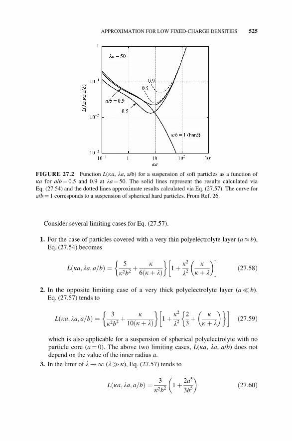
FIGURE 27.3 A cell model for a concentrated suspension of porous spheres. Each porous

sphere of radius a is surrounded by a virtual shell of outer radius b. The particle volume

fraction � is given by �¼ (a/b)3.


surface potential co, which becomes for large ka (Eq. (4.29))

co ¼ZeN

2ereok2ð27:63Þ

is proportional to 1/k2 so that for large ka, Eq. (27.54) becomes

p ¼ ðZNÞ220Zl2

PMi¼1

z2i n1i li

� �PMi¼1

z2i n1i

� �2ð27:64Þ

Equation (27.64) shows that the electroviscous coefficient p for large kadecreases with increasing ka.

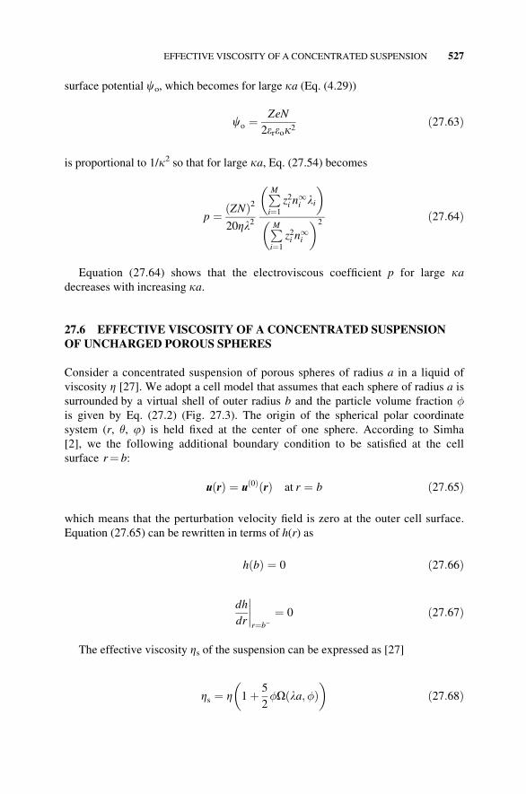
27.6 EFFECTIVE VISCOSITY OF A CONCENTRATED SUSPENSIONOF UNCHARGED POROUS SPHERES

Consider a concentrated suspension of porous spheres of radius a in a liquid of

viscosity Z [27]. We adopt a cell model that assumes that each sphere of radius a is

surrounded by a virtual shell of outer radius b and the particle volume fraction �is given by Eq. (27.2) (Fig. 27.3). The origin of the spherical polar coordinate

system (r, �, j) is held fixed at the center of one sphere. According to Simha

[2], we the following additional boundary condition to be satisfied at the cell

surface r¼ b:

uðrÞ ¼ uð0ÞðrÞ at r ¼ b ð27:65Þ

which means that the perturbation velocity field is zero at the outer cell surface.

Equation (27.65) can be rewritten in terms of h(r) as

hðbÞ ¼ 0 ð27:66Þ

dh

dr

��r¼b�

¼ 0 ð27:67Þ

The effective viscosity Zs of the suspension can be expressed as [27]

Zs ¼ Z 1þ 5

2�Oðla; �Þ

� �ð27:68Þ

EFFECTIVE VISCOSITY OF A CONCENTRATED SUSPENSION 527

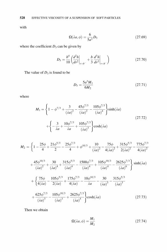
with

Oðla; �Þ ¼ 6

5a3D3 ð27:69Þ

where the coefficient D3 can be given by

D3 ¼ b4

10

d2h

dr2

��r¼b�

þ b

3

d3h

dr3

��r¼b�

� �ð27:70Þ

The value of D3 is found to be

D3 ¼ 5a3M1

6M2

ð27:71Þ

where

M1 ¼ 1� �7=3 þ 3

ðlaÞ2 �45�7=3

ðlaÞ2 � 105�7=3

ðlaÞ4( )

sinhðlaÞ

þ � 3

laþ 10�7=3

laþ 105�7=3

ðlaÞ3( )

coshðlaÞ

ð27:72Þ

M2 ¼ 1� 25�

4

�þ 21�5=3

2� 25�7=3

4þ �10=3 þ 10

ðlaÞ2 �75�

4ðlaÞ2 þ315�5=3

2ðlaÞ2 � 775�7=3

4ðlaÞ2

þ 45�10=3

ðlaÞ2 þ 30

ðlaÞ4 þ315�5=3

ðlaÞ4 � 1500�7=3

ðlaÞ4 þ 105�10=3

ðlaÞ4 � 2625�7=3

ðlaÞ6)

sinhðlaÞ

þ 75�

4ðlaÞ�

� 105�5=3

2ðlaÞ þ 175�7=3

4ðlaÞ � 10�10=3

la� 30

ðlaÞ3 �315�5=3

ðlaÞ3

þ 625�7=3

ðlaÞ3 � 105�10=3

ðlaÞ3 þ 2625�7=3

ðlaÞ5)coshðlaÞ ð27:73Þ

Then we obtain

Oðla; �Þ ¼ M1

M2

ð27:74Þ


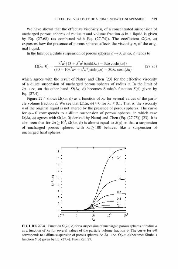
We have shown that the effective viscosity Zs of a concentrated suspension of

uncharged porous spheres of radius a and volume fraction � in a liquid is given

by Eq. (27.68) (as combined with Eq. (27.74)). The coefficient O(la, �)expresses how the presence of porous spheres affects the viscosity Zs of the orig-inal liquid.

In the limit of a dilute suspension of porous spheres �! 0, O(la, �) tends to

Oðla; 0Þ ¼ l2a2fð3þ l2a2ÞsinhðlaÞ � 3la coshðlaÞgð30þ 10l2a2 þ l4a4ÞsinhðlaÞ � 30la coshðlaÞ ð27:75Þ

which agrees with the result of Natraj and Chen [23] for the effective viscosity

of a dilute suspension of uncharged porous spheres of radius a. In the limit of

la!1, on the other hand, O(la, �) becomes Simha’s function S(�) given by

Eq. (27.4).

Figure 27.4 shows O(la, �) as a function of la for several values of the parti-

cle volume fraction �. We see that O(la, �)� 0 for la 0.1. That is, the viscosity

Z of the original liquid is not altered by the presence of porous spheres. The curve

for �¼ 0 corresponds to a dilute suspension of porous spheres, in which case

O(la, �) agrees with O(la, 0) derived by Natraj and Chen (Eq. (27.75)) [23]. It is

also seen that for la� 103, O(la, �) is almost equal to S(�) so that a suspension

of uncharged porous spheres with la� 100 behaves like a suspension of

uncharged hard spheres.

FIGURE 27.4 Function O(la, �) for a suspension of uncharged porous spheres of radius aas a function of la for several values of the particle volume fraction �. The curve for � 0

corresponds to a dilute suspension of porous spheres. As la!1, O(la, �) becomes Simha’s

function S(�) given by Eq. (27.4). From Ref. 27.

EFFECTIVE VISCOSITY OF A CONCENTRATED SUSPENSION 529

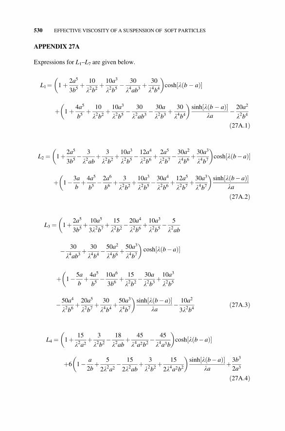
APPENDIX 27A

Expressions for L1–L7 are given below.

L1¼ 1þ 2a5

3b5þ 10

l2b2þ 10a3

l2b5� 30

l4ab3þ 30

l4b4

� �cosh lðb� aÞ½ �

þ 1þ 4a5

b5þ 10

l2b2þ 10a3

l2b5� 30

l2ab3� 30a

l2b3þ 30

l4b4

� �sinh½lðb� aÞ�

la� 20a2

l2b4

ð27A:1Þ

L2 ¼ 1þ 2a5

3b5� 3

l2abþ 3

l2b2þ 10a3

l2b5� 12a4

l2b6þ 2a5

l2b7� 30a2

l4b6þ 30a3

l4b7


þ 1� 3a

bþ 4a5

b5� 2a6

b6þ 3

l2b2þ 10a3

l2b5� 30a4

l2b6þ 12a5

l2b7þ 30a3

l4b7


la

ð27A:2Þ

L3 ¼ 1þ 2a5

3b5

�þ 10a5

3l2b7þ 15

l2b2� 20a4

l2b6þ 10a3

l2b5� 5

l2ab

� 30

l4ab3þ 30

l4b4� 50a2

l4b6þ 50a3

l4b7

�cosh lðb� aÞ½ �

þ 1� 5a

b

�þ 4a5

b5� 10a6

3b6þ 15

l2b2� 30a

l2b3þ 10a3

l2b5

�50a4

l2b6þ 20a5

l2b7þ 30

l4b4þ 50a3

l4b7

�sinh½lðb� aÞ�

la� 10a2

3l2b4ð27A:3Þ

L4 ¼ 1þ 15

l2a2þ 3

l2b2� 18

l2abþ 45

l4a2b2� 45

l4a3b


þ6 1� a

2bþ 5

2l2a2� 15

2l2abþ 3

l2b2þ 15

2l4a2b2


laþ 3b3

2a3

ð27A:4Þ


L5ðrÞ¼ 1þ2a5

3b5þ 3

l2r2� 3

l2raþ10a3

l2b5þ 2a5

l2r2b5� 12a4

l2rb5� 30a2

l4rb5þ 30a3

l4r2b5

� �cosh lðr�aÞ½ �

þ 1þ4a5

b5�2a6

rb5�3a

rþ10a3

l2b5þ 3

l2r2þ 12a5

l2r2b5� 30a4

l2rb5þ 30a3

l4r2b5

� �sinh½lðr�aÞ�

la

ð27A:5Þ

L6¼ 1� 3

l2abþ 3

l2b2

� �cosh lðb�aÞ½ �þ 1�3a

bþ 3

l2b2

� �sinh½lðb�aÞ�

la�a2

b2

ð27A:6Þ

L7ðrÞ ¼ 1�b

r� 3

l2rbþ 3

l2r2

� �cosh lðr�bÞ½ �

þ 1þl2b2

3þ 3

l2r2þb2

r2�3b

r

� �sinh½lðr�bÞ�

lb

ð27A:7Þ

REFERENCES

1. A. Einstein, Ann. Phys. 19 (1906) 289.

2. R. J. Simha, Appl. Phys. 23 (1952) 1020.

3. M. Smoluchowski, Kolloid Z. 18 (1916) 194.

4. W. Krasny-Ergen, Kolloidzeitschrift 74 (1936) 172.

5. F. Booth, Proc. R. Soc. A 203 (1950) 533.

6. W. B. Russel, J. Fluid Mech. 85 (1978) 673.

7. D. A. Lever, J. Fluid Mech. 92 (1979) 421.

8. D. J. Sherwood, J. Fluid Mech. 101 (1980) 609.

9. I. G. Watterson and L. R. White, J. Chem. Soc., Faraday Trans. 2 77 (1981) 1115.

10. E. J. Hinch and J. D. Sherwood, J. Fluid Mech. 132 (1983) 337.

11. A. S. Duhkin and T. G. M. van de Ven, J. Colloid Interface Sci. 158 (1993) 85.

12. F. J. Rubio-Hern�andez, E. Ruiz-Reina, and A. I. G�omez-Merino, J. Colloid Interface Sci.206 (1998) 334.

13. F. J. Rubio-Hern�andez, E. Ruiz-Reina, and A. I. G�omez-Merino, J. Colloid Interface Sci.226 (2000) 180.

14. J. D. Sherwood, F. J. Rubio-Hern�andez, and E. Ruiz-Reina, J. Colloid Interface Sci. 228(2000) 7.

15. F. J. Rubio-Hern�andez, E. Ruiz-Reina, and A. I. G�omez-Merino, Colloids Surf. A: Phys-icochem. Eng. Aspects 192 (2001) 349.

16. F. J. Rubio-Hern�andez, E. Ruiz-Reina, A. I. G�omez-Merino, and J. D. Sherwood, Rheol.Acta 40 (2001) 230.

REFERENCES 531

17. H. Ohshima, Langmuir 22 (2006) 2863.

18. H. Ohshima, Theory of Colloid and Interfacial Electric Phenomena, Academic Press,

Amsterdam, 2006.

19. E. Ruiz-Reina, F. Carrique, F. J. Rubio-Hern�andez, A. I. G�omez-Merino, and P.

Garc�ia-S�anchez, J. Phys. Chem. B 107 (2003) 9528.

20. F. J. Rubio-Hern�andez, F. Carrique, and E. Ruiz-Reina, Adv. Colloid Interface Sci. 107(2004) 51.


22. G. I. Taylor, Proc. R. Soc. London, Ser. A 138 (1932) 41.

23. V. Natraj and S. B. Chen, J. Colloid Interface Sci. 251 (2002) 200.

24. S. Allison, S. Wall, and M. Rasmusson, J. Colloid Interface Sci. 263 (2003) 84.

25. S. Allison and Y. Xin, J. Colloid. Interface. Sci. 299 (2006) 977.


27. H. Ohshima, Colloids Surf. A: Physicochem. Eng. Aspects 347 (2009) 33.


Documents

Biophysical Chemistry of Biointerfaces (Ohshima/Biophysical Chemistry of Biointerfaces) || Effective Viscosity of a Suspension of Soft Particles