Embed Size (px)
Citation preview

6 Potential DistributionAround a Charged Particle ina Salt-Free Medium
6.1 INTRODUCTION
The potential distribution around a charged colloidal particle in an electrolyte solu-
tion, which plays an essential role in various electric phenomena observed in colloi-
dal suspensions, can be described by the Poisson–Boltzmann equation. Consider a
particle carrying ionized groups on the particle surface in an electrolyte solution. In
the suspension, in addition to electrolyte ions, there are counterions produced by
dissociation of the particle surface groups. The following two assumptions are usu-
ally made: (i) the concentration of counterions from the surface groups can be ne-
glected as compared with the electrolyte concentration and (ii) the suspension is
assumed to be infinitely dilute so that any effects resulting from the finite particle
volume fraction can be neglected. The assumption (i) becomes invalid where the
electrolyte concentration is as low as or lower than that of counterions from
the particle. The assumption (ii) does not hold when the concentration of all ions
(electrolyte ions and counterions from the particle) is very low, since in this case
the potential around each particle becomes quite long range and the effects of the
finite particle volume fraction become appreciable.
The Poisson–Boltzmann equation for the potential distribution around a cylindri-
cal particle without recourse to the above two assumptions for the limiting case of
completely salt-free suspensions containing only particles and their counterions was
solved analytically by Fuoss et al. [1] and Afrey et al. [2]. As for a spherical parti-
cle, although the exact analytic solution was not derived, Imai and Oosawa [3,4]
studied the analytic properties of the Poisson–Boltzmann equation for dilute parti-
cle suspensions. The Poisson–Boltzmann equation for a salt-free suspension has re-
cently been numerically solved [5–8].
The above theories, however, is based on an idealized model assuming that
there are only counterions from the particle and no other ions. Actually, even
salt-free media may contain other ions rather than counterions from the particle
surface groups. Salt-free water at pH 7, for example, contains 10�7M H+ and OH�
ions. It is thus of interest to examine how the above behaviors of colloidal particles
Biophysical Chemistry of Biointerfaces By Hiroyuki OhshimaCopyright# 2010 by John Wiley & Sons, Inc.
132

in a salt-free medium are influenced if a small amount of salts is added to the me-
dium. In their second paper [4], Imai and Oosawa studied the analytic properties of
the Poisson–Boltzmann equation in the presence of added salts, which are found to
exhibit similar behaviors to those of completely salt-free suspensions.
In this chapter, we first discuss the case of completely salt-free suspensions of
spheres and cylinders. Then, we consider the Poisson–Boltzmann equation for the
potential distribution around a spherical colloidal particle in a medium containing
its counterions and a small amount of added salts [8]. We also deals with a soft
particle in a salt-free medium [9].
6.2 SPHERICAL PARTICLE
Consider a dilute suspension of spherical colloidal particles of radius a with a sur-
face charge density s or the total surface charge Q¼ 4pa2s in a salt-free medium
containing only counterions. We assume that each sphere is surrounded by a con-
centric spherical cell of radius R [5,7] (Fig. 6.1), within which counterions are dis-
tributed so that electrical neutrality as a whole is satisfied. The particle volume
fraction � is given by
� ¼ ða=RÞ3 ð6:1Þ
We treat the case of dilute suspensions, namely,
� � 1 or a=R � 1 ð6:2Þ
FIGURE 6.1 A spherical particle of radius a in a free volume of radius R. (a/R)3 equalsthe particle volume fraction �.
SPHERICAL PARTICLE 133

We denote the electric potential at a distance r from the center O of one particle by
c(r). Let the average number density and the valence of counterions be n and �z,respectively. Then we have
Q ¼ 4pa2s ¼ 4
3pðR3 � a3Þzen ð6:3Þ
We set the electric potential c(r) to zero at points where the volume charge density
r(r) resulting from counterions equals its average value (�zen). We assume that the
distribution of counterions obeys a Boltzmann distribution, namely,
rðrÞ ¼ �zen exp ��zecðrÞkT
� �¼ �zen exp
zecðrÞkT
� �ð6:4Þ
The Poisson equation for the electric potential c(r) around the particle is
given by
d2cðrÞdr2
þ 2
r
dcðrÞdr
¼ � rðrÞereo
ð6:5Þ
where er is the relative permittivity of the medium. By combining Eqs. (6.4) and
(6.5), we obtain the following spherical Poisson–Boltzmann equation for a salt-free
system:
d2y
dr2þ 2
r
dy
dr¼ k2ey ð6:6Þ
where
yðrÞ ¼ zecðrÞkT
ð6:7Þ
is the scaled potential and
k ¼ z2e2n
ereokT
� �1=2
¼ ze
ereokT� 3a2sðR3 � a3Þ
� �1=2¼ 3zeQ
4pereokTðR3 � a3Þ� �1=2
¼ffiffiffiffiffiffiffiffiffiffiffiffiffiffiffi3Q�aR3 � a3
r
ð6:8Þ
is the Debye–H€uckel parameter in the present system. Here
Q� ¼ ze
kT� Q
4pereoað6:9Þ
134 POTENTIAL DISTRIBUTION AROUND A CHARGED PARTICLE

is the scaled particle charge. For the dilute case (a/R� 1), Eq. (6.8) becomes
k ¼ 3zea2sereokTR3
� �1=2¼ 3zeQ
4pereokTR3
� �1=2¼
ffiffiffiffiffiffiffiffiffiffiffi3Q�aR3
rð6:10Þ
Note that the right-hand side of Eq. (6.6) contains only one term resulting from
counterions, unlike the usual Poisson–Boltzmann equation. Since s (or Q) and z areof the same sign, the product zs (or zQ) is always positive. Note that k depends on s(or Q), a, and R unlike the case of salt solutions, where k is essentially independent
of these parameters.
The boundary conditions are expressed as
dcdr
����r¼a
¼ � sereo
¼ � Q
4pereoa2¼ � kT
ze� Q
�
að6:11Þ
dcdr
����r¼R
¼ 0 ð6:12Þ
which can be rewritten in terms of y and k as
dy
dr
����r¼a
¼ �Q�
a¼ � k2ðR3 � a3Þ
3a2ð6:13Þ
dy
dr
����r¼R
¼ 0 ð6:14Þ
For the dilute case, Eq. (6.13) becomes
dy
dr
����r¼a
¼ � k2R3
3a2ð6:15Þ
Also from Eqs. (6.6) and (6.13) we have
Z R
a
eyr2 dr ¼ 1
3ðR3 � a3Þ ð6:16Þ
Equation (6.6) cannot be solved analytically but its approximate solution for the
case of dilute suspensions has been obtained by Imai and Oosawa [3,4]. They
showed that there are two distinct cases separated by a certain critical value of the
surface charge density s or the total surface charge Q, that is, case 1: low surface
charge density case and case 2: high surface charge density case, as schematically
shown in Fig. 6.2. For case 1, there are two regions I (R�� r�R) and II (a� r�R�),while for case II, there are three regions I (R�� r�R), II (a�� r�R�), and III
SPHERICAL PARTICLE 135

(a� r� a�). That is, for case 1, a� reduces to a so that region III disappears. Note
that counter-ion condensation occurs in the vicinity of the particle surface, that is,
in region III because of very strong electric field there. This is a characteristic of a
salt-free system.
Since in region I (far from the particle), the potential y(r) is almost equal to y(R),which is the potential at the outer boundary of the free volume of radius R, thePoisson–Boltzmann equation (6.6) can be approximated by
d2y
dr2þ 2
r
dy
dr¼ k2eyðRÞ ð6:17Þ
Rar
R*a*0
IIIIII
ψ (r)
Case 2
ψ (a)
ψ (R)
Counter-ion condensation
ψ (a)
Ra rψ (R)
R*0
III
ψ (r)
Case 1
ψ (r) ≅ constantψ (r)∝1/r
Surface
Surface
FIGURE 6.2 Three possible regions I, II, and III of r around a sphere of radius a. Forcase 1 (low surface charge densities), there are two regions I (R�� r�R) and II (a� r�R�),whereas for case 2 (high surface charge densities), there are three regions I (R�� r�R),II (a�� r�R�), and III (a� r� a�). Counterions are condensed in region III (counter-ion con-
densation). The particle surface potential co is defined by co�c(a)�c(R). From Ref. [5].
136 POTENTIAL DISTRIBUTION AROUND A CHARGED PARTICLE

which, subject to Eq. (6.12), can be solved to give
yðrÞ ¼ Q� areyðRÞ 1þ r3
2R3� 3r
2R
� �þ yðRÞ; ðR� � r � RÞ ð6:18Þ
In the dilute case (a/R� 1), as r decreases to R�, approaching region II, the term
proportional to 1/r in Eq. (6.18) becomes dominant. Since y(r) must be continuous
at r¼R�, y(r) in region II (a� r�R� for case 1 and a�� r�R� for case 2) shouldbe of the form
yðrÞ ¼ Q� areyðRÞ þ yðRÞ ð6:19Þ
which satisfies
d2y
dr2þ 2
r
dy
dr¼ 0 ð6:20Þ
We now introduce
xðrÞ ¼ � 1
k2r� dydr
e�y ð6:21Þ
which is related to the ratio of the second term on the left-hand side to the right-
hand side of Eq. (6.6). Since Eq. (6.6) tends to Eq. (6.20) when x(r)� 1, we see
that the condition
xðrÞ � 1 ð6:22Þ
must hold in region II.
We evaluate x(r) at r¼ a� from Eqs. (6.19) and (6.21) and obtain
xða�Þ ¼ 1
3
R
a�
� �3
exp� yða�Þ � yðRÞf g½ � ð6:23Þ
which yields
yða�Þ � yðRÞ ¼ 3 lnR
a�
� �� lnð3xða�ÞÞ ð6:24Þ
Since x(a�)� 1 (Eq. (6.22)), we find that
yða�Þ � yðRÞ � 3 lnR
a�
� �ð6:25Þ
SPHERICAL PARTICLE 137

which implies that the value of y(a�)� y(R) cannot exceed 3 ln(R/a�) for the dilutecase. In other words, the maximum value of y(a�)� y(R) is 3 ln(R/a�). FromEq. (6.19), on the other hand, it follows that, for the dilute case,
yða�Þ � yðRÞ ¼ �rdy
dr
����r¼a�
ð6:26Þ
By combining Eqs. (6.25) and (6.26), we obtain
�dy
dr
����r¼a�
� 3
a�ln
R
a�
� �ð6:27Þ
We must thus consider two separate cases 1 and 2, depending on whether
�dy=drjr¼a is larger or smaller than (3/a)ln(R/a).
(a) Case 1 (low surface charge case). Consider first case 1, in which case the
following condition holds:
�dy
dr
����r¼a
� 3
aln
R
a
� �ð6:28Þ
By using Eq. (6.15) (for the dilute case), Eq. (6.28) can be rewritten as
ðkaÞ2 � 3� lnð1=�Þ ð6:29Þ
or by using Eq. (6.9)
Q� � lnð1=�Þ ð6:30Þ
In this case, region II can extend up to r¼ a, that is, a� can reduce to a. Thus,the entire region of r can be covered only with regions I and II and one does
not need region III. For the low surface charge case (small k), Eq. (6.6) canbe approximated by
d2y
dr2þ 2
r
dy
dr¼ k2 ¼ 3Q�
R3ð6:31Þ
with the solution
yðrÞ ¼ Q� ar
1þ r3
2R3� 3r
2R
� �þ yðRÞ; ða � r � RÞ ð6:32Þ
which is now applicable for the entire region of r. One can determine the
value of y(R) in Eq. (6.32) to satisfy Eq. (6.16) (in which ey may be approxi-
mated by 1 + y). The result for the dilute case is
138 POTENTIAL DISTRIBUTION AROUND A CHARGED PARTICLE

yðRÞ ¼ � k2R2
10¼ �Q�a
10Rð6:33Þ
Thus, Eq. (6.32) becomes
yðrÞ ¼ Q� ar
1þ r3
2R3� 9r
5R
� �; ða � r � RÞ ð6:34Þ
and
yðRÞ 0 for � � 1 ð6:35Þ
Note that Eq. (6.34) satisfies Eq. (6.12). From Eq. (6.34) we obtain
yðaÞ ¼ Q� 1þ a3
2R3� 9a
5R
� � Q� ð6:36Þ
We define the particle surface potential co as the potential c(a) at r¼ aminus the potential c(R) at r¼R, that is, co¼c(a)�c(R). The scaled sur-
face potential of the particle yo� zeco/kT is thus given by yo¼ y(a)� y(R).From Eqs. (6.35) and (6.36), we obtain for the dilute case
yo ¼ Q� ð6:37Þ
that is,
co ¼Q
4pereoað6:38Þ
Note that Eq. (6.37) (or Eq. (6.38)) does not depend on the particle volume
fraction � and coincides with the surface potential of a sphere of radius acarrying a total charge Q¼ 4pa2s for the limiting case of k! 0, expressed
by an unscreened Coulomb potential. That is, the surface potential in this
case is the same as if the counterions were absent.
(b) Case 2 (high surface charge case). Consider next case 2, in which case the
condition
�dy
dr
����r¼a
>3
aln
R
a
� �ð6:39Þ
which can be rewritten as
ðkaÞ2 > 3� lnð1=�Þ ð6:40Þ
SPHERICAL PARTICLE 139
or
Q� > lnð1=�Þ ð6:41Þ
Thus, in this case, we find that
�dy
dr
����r¼a
> �dy
dr
����r¼a�
ð6:42Þ
That is, region II cannot extend up to r¼ a. Therefore, the entire region of rcannot be covered only with regions I and II and thus one needs region III
very near the particle surface between r¼ a and r¼ a�. In region III, the
term k2ey in Eq. (6.6) becomes very large so that x(r)� 1. The Poisson–
Boltzmann equation in region III thus becomes
d2y
dr2¼ k2ey ð6:43Þ
which is of the same form as the Poisson–Boltzmann equation for a planar
surface. Integration of Eq. (6.43) after multiplying dy/dr on both sides gives
1
2
dy
dr
� �2
¼ k2ey þ C ð6:44Þ
C being an integration constant. For high potentials, Cmay be ignored so that
Eq. (6.44) yields
dy
dr¼ �
ffiffiffi2
pkey=2 ð6:45Þ
By evaluating Eq. (6.45) at r¼ a and using Eq. (6.15), we obtain for the
dilute case
yðaÞ ¼ lnk2R6
18a4
� �¼ ln
1
6�
ze
kT
� � Q
4pereoa
� �� �¼ ln
Q�
6�
� �ð6:46Þ
The value of y(R) can be obtained as follows. In case 2, y(a�)� y(R) hasalready reached its maximum 3 ln(R/a�). Thus from Eq. (6.19) we have
k2R3
3a�exp yðRÞ½ � ¼ 3 ln
R
a�
� �ð6:47Þ
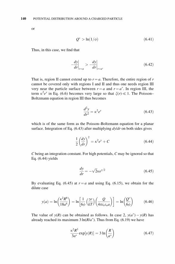
140 POTENTIAL DISTRIBUTION AROUND A CHARGED PARTICLE

so that Eq. (6.19) becomes
yðrÞ ¼ 3 lnR
a�
� �a�
rþ yðRÞ; ða� � r � RÞ ð6:48Þ
The value of y(R) in case 2 can be obtained from Eq. (6.46). For the purpose
of determining y(R) from Eq. (6.47), one may replace a� by a in Eq. (6.47)
so that
yðRÞ ¼ �lnðkaÞ2
9 lnðR=aÞR
a
� �3" #
¼ �ln1
lnð1=�Þze
kT
� � Q
4pereoa
� �� �
¼ �lnQ�
lnð1=�Þ� � ð6:49Þ
From Eqs. (6.46) and (6.49), we find that the scaled particle surface potential
ys¼ y(a)� y(R) in case 2 is given by
yo ¼ lnðkaÞ4
162 lnðR=aÞR
a
� �9" #
¼ ln1
6�lnð1=�Þze
kT
� �2 Q
4pereoa
� �2" #
¼ lnðQ�Þ2
6� lnð1=�Þ
" # ð6:50Þ
that is, co¼c(a)�c(R) in case 2 is given by
co ¼kT
zeln
1
6� lnð1=�Þze
kT
� �2 Q
4pereoa
� �2" #
¼ kT
zeln
ðQ�Þ26� lnð1=�Þ
" #ð6:51Þ
Note that Eq. (6.51) implies that c0 depends less on Q than Eq. (6.38) and
that co is a function of the particle volume fraction �.We introduce the effective surface potential ceff and the effective surface
charge Qeff defined by
ceff ¼kT
ze
� �lnð1=�Þ ð6:52Þ
Qeff ¼ 4pereoakT
ze
� �lnð1=�Þ ð6:53Þ
and the corresponding dimensionless quantities yeff and Q�eff
yeff ¼ lnð1=�Þ ð6:54Þ
SPHERICAL PARTICLE 141

Q�eff ¼
Qeff
4pereoaze
kT
� �¼ lnð1=�Þ ð6:55Þ
That is, yeff¼Q�eff . Then the potential distribution around the particle except
the region very near the particle surface is approximately given by
cðrÞ ¼ ceff
a
rþ yðRÞ ¼ Qeff
4pereorþ yðRÞ; ða� � r � RÞ ð6:56Þ
or
yðrÞ ¼ yeffa
rþ yðRÞ ¼ Q�
eff
a
rþ yðRÞ; ða� � r � RÞ ð6:57Þ
We thus see that for case 2 (high surface charge case), the particle behaves like a
sphere showing a Coulomb potential with the effective surface charge Qeff except
the region very near the particle surface (a�� r�R).We compare the exact numerical solution to the Poisson–Boltzmann equation
(6.6) and the approximate results, Eq. (6.37) for case 1 (low surface charge density
case) and Eq. (6.50) for case 2 (high surface charge density case) in Fig. 6.3, in
which the scaled surface potential yo� zeco/kT is plotted as a function of the scaled
FIGURE 6.3 Scaled surface potential yo¼ zeco/kT, defined by yo� y(a)� y(R) of a sphereof radius a, as a function of the scaled total surface charge Q� = (ze/kT)Q/4pereoa for various
values of the particle volume fraction �. Solid lines represent exact numerical results. The
dashed line, which passes through the origin (yo¼ 0 and Q�¼ 0), is approximate results calcu-
lated by an unscreened Coulomb potential, Eq. (6.37) (case 1: low surface charge densities)
and dotted lines by Eq. (6.50) (case 2: high surface charge densities). Closed circles corre-
spond to the approximate critical values of Q� separating cases 1 and 2, given by Eq. (6.58).
142 POTENTIAL DISTRIBUTION AROUND A CHARGED PARTICLE

total surface charge Q� for various values of the particle volume fraction �. Notethat yo is always positive. The agreement between the exact results and the approxi-
mate results is excellent with negligible errors except in the transition region
between cases 1 and 2. It follows from the conditions for case 1 (Eq. (6.30)) and
case 2 (Eq. (6.41)) that an approximate expression for the critical value of Q sepa-
rating cases 1 and 2 for dilute suspensions is given by
Q� ¼ lnð1=�Þ ð6:58Þ
6.3 CYLINDRICAL PARTICLE
Consider a dilute suspension of parallel cylindrical particles of radius a with a sur-
face charge density s or total surface charge Q¼ 2pas per unit length in a salt-free
medium containing only counterions. We assume that each cylinder is surrounded
by a cylindrical free volume of radius R, within which counterions are distributed sothat electroneutrality as a whole is satisfied. We define the particle volume fraction
� as
� ¼ ða=RÞ2 ð6:59Þ
The cylindrical particles are assumed to be parallel and equidistant. We treat the
case of dilute suspensions, namely, �� 1 or a/R� 1. Let the average number den-
sity and the valence of counterions in the absence of the applied electric field be nand �z, respectively. Then we have
Q ¼ 2pas ¼ pðR2 � a2Þzen ð6:60Þ
We set the equilibrium electric potential c(0)(r) (where r is the distance from the
axis of one cylinder) to zero at points where the volume charge density resulting
from counterions equals its average value (�zen). We assume that the distribution
of counterions obeys a Boltzmann distribution (Eq. (6.4)). The cylindrical Poisson–
Boltzmann equation thus becomes
d2y
dr2þ 1
r
dy
dr¼ k2ey ð6:61Þ
with
k ¼ z2e2n
ereokT
� �1=2
¼ ze
ereokT� 2asðR2 � a2Þ
� �1=2¼ zeQ
pereokTðR2 � a2Þ� �1=2
ð6:62Þ
where y(r)¼ zec(r)/kT is the scaled equilibrium potential and k is the Debye–
H€uckel parameter in the present system. The boundary conditions are
CYLINDRICAL PARTICLE 143

dcdr
����r¼a
¼ � sereo
¼ � Q
2pereoað6:63Þ
dcdr
����r¼R
¼ 0 ð6:64Þ
The Poisson–Boltzmann equation (6.61) subject to boundary conditions (6.63)
and (6.64) has been solved independently by Fuoss et al. [1] and Afrey et al. [2].
The results are given below.
(a) Case 1 (low surface charge case). If the condition
0 < Q� <lnða=RÞ
lnða=RÞ � 1ð6:65Þ
is satisfied, then we have
yðaÞ ¼ �lnk2a2
2� 1
ð1� Q�Þ2 � b2
" #ð6:66Þ
yðRÞ ¼ �lnk2R2
2� 1
1� b2
� �ð6:67Þ
where Q� is a scaled particle charge per unit length defined by
Q� ¼ Q
4pereo� zekT
ð6:68Þ
(Note that Q� is always positive, since Q and z are always of the same sign)
and b is given by the solution to the following transcendental equation:
Q� ¼ 1� b2
1� b cothfb lnða=RÞg ð6:69Þ
(b) Case 2 (high surface charge case). If the condition
Q� lnða=RÞlnða=RÞ � 1
ð6:70Þ
144 POTENTIAL DISTRIBUTION AROUND A CHARGED PARTICLE
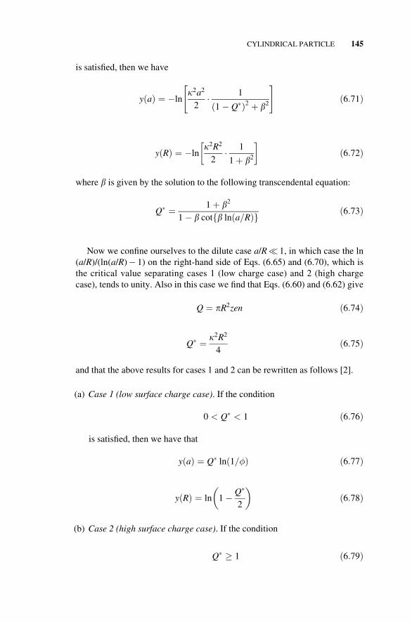
is satisfied, then we have
yðaÞ ¼ �lnk2a2
2� 1
ð1� Q�Þ2 þ b2
" #ð6:71Þ
yðRÞ ¼ �lnk2R2
2� 1
1þ b2
� �ð6:72Þ
where b is given by the solution to the following transcendental equation:
Q� ¼ 1þ b2
1� b cotfb lnða=RÞg ð6:73Þ
Now we confine ourselves to the dilute case a/R� 1, in which case the ln
(a/R)/(ln(a/R)� 1) on the right-hand side of Eqs. (6.65) and (6.70), which is
the critical value separating cases 1 (low charge case) and 2 (high charge
case), tends to unity. Also in this case we find that Eqs. (6.60) and (6.62) give
Q ¼ pR2zen ð6:74Þ
Q� ¼ k2R2
4ð6:75Þ
and that the above results for cases 1 and 2 can be rewritten as follows [2].
(a) Case 1 (low surface charge case). If the condition
0 < Q� < 1 ð6:76Þ
is satisfied, then we have that
yðaÞ ¼ Q� lnð1=�Þ ð6:77Þ
yðRÞ ¼ ln 1� Q�
2
� �ð6:78Þ
(b) Case 2 (high surface charge case). If the condition
Q� 1 ð6:79Þ
CYLINDRICAL PARTICLE 145

is satisfied, then we have that
yðaÞ ¼ lnQ�
2�
� �ð6:80Þ
yðRÞ ¼ �lnð2Q�Þ ð6:81Þ
Further, if we define the particle surface potential co as co¼c(a)�c(R)or the scaled surface potential yo� (ze/kT)co as yo¼ y(a)� y(R), then we
obtain for the dilute case
yo ¼ Q� lnð1=�Þ; for 0 < Q� < 1 ðcase 1: low surface charge caseÞð6:82Þ
yo ¼ lnQ�2
�
� �; forQ� 1 ðcase 2: high surface charge caseÞ ð6:83Þ
Equation (6.82) agrees with the unscreened Coulomb potential of a
charged cylinder. That is, the surface potential in this case is the same as
if the counterions were absent.
6.4 EFFECTS OF A SMALL AMOUNT OF ADDED SALTS
We consider a suspension of spherical colloidal particles of radius a with mono-
valent ionized groups on their surface in a medium which contains counterions pro-
duced by dissociation of the particle surface groups and a small amount of
monovalent symmetrical electrolytes [8]. We may assume that the particles are pos-
itively charged without loss of generality. We treat the case in which N ionized
groups of valence +1 are uniformly distributed on the surface of each particle and Ncounterions of valence �1 are produced by dissociation of the particle surface
groups. Each particle thus carries a charge Q¼ eN, where e is the elementary elec-
tric charge. We also assume that each particle is surrounded by a spherical free vol-
ume of radius R (Fig. 6.1), within which electroneutrality as a whole is satisfied.
The particle volume fraction � is given by �¼ (a/R)3. We treat the case of dilute
(but not infinitely dilute) suspensions, namely, �� 1 or a/R� 1. We assume that
the electrolyte is completely dissociated to give M cations of valence +1 and Manions of valence �1 in each free volume so that there are N+M counterions and
M coions in the free volume. Let the average concentration (number density) of
total counterions be n+m and that of anions be m, n and m being given by
n ¼ N
V; m ¼ M
Vð6:84Þ
146 POTENTIAL DISTRIBUTION AROUND A CHARGED PARTICLE

where
V ¼ 4
3pðR3 � a3Þ ð6:85Þ
is the volume available for counterions and coions within each free volume. From
the condition of electroneutrality in each free volume, we have
Q ¼ eN ¼ Ven ð6:86Þ
We assume that the equilibrium distribution of ions obeys a Boltzmann distribu-
tion so that volume charge density r(r) at position r, r being the distance from the
particle center (r a), is given by
rðrÞ ¼ e �ðnþ mÞey V
4pR R
a eyr2 drþ mey
V
4pR R
a e�yr2 dr
" #ð6:87Þ
where y(r)¼ ec(r)/kT is the scaled potential. Note that Eq. (6.87) satisfies the elec-
troneutrality condition of a free volume, namely,
4pZ R
a
rðrÞr2dr ¼ ef�ðN þMÞ þMg ¼ �eN ¼ �Q ð6:88Þ
We set the electric potential c(r) to zero at points where the concentration of total
counterions equals its average value nþm so that
4pZ R
a
eyr2dr ¼ V ¼ 4p3ðR3 � a3Þ ð6:89Þ
and Eq. (6.87) becomes
rðrÞ ¼ en �ð1þ pÞey þ p
We�y
h ið6:90Þ
with
W ¼ 4pR Ra e�yr2 dr
V¼
R Ra e�yr2 dr
ðR3 � a3Þ=3 ð6:91Þ
and
p ¼ m
nð6:92Þ
EFFECTS OF A SMALL AMOUNT OF ADDED SALTS 147

where p is the ratio of the concentration of counterions (or coions) resulting from
the added electrolytes to that of counterions from the particle. The case of p¼ 0
corresponds to the completely salt-free case.
By combining the Poisson equation (6.5) and Eq. (6.87), we obtain the following
Poisson–Boltzmann equation for the equilibrium electric potential c(r) at positionr, r being the distance from the particle center (r a):
d2y
dr2þ 2
r
dy
dr¼ k2
1þ 2pð1þ pÞey � p
We�y
h ið6:93Þ
where k is the Debye–H€uckel parameter defined by
k ¼ e2ðnþ 2mÞereokT
� �1=2¼ 3Q��ð1þ 2pÞ
a2ð1� �Þ� �1=2
ð6:94Þ
and
Q� ¼ Q
4pereoae
kT
� �¼ k2a2ð1� �Þ
3�ð1þ 2pÞ ð6:95Þ
is the scaled particle charge. Note that k generally depends on Q�, p, a, and � and
that when n�m, k becomes the usual Debye–H€uckel parameter of a 1–1 electro-
lyte of concentration m, given by
k ¼ 2e2m
ereokT
� �1=2
ð6:96Þ
The boundary conditions are the same as Eqs. (6.11) and (6.12).
We derive some approximate solutions to Eq. (6.93). It can be shown that as in
the case of completely salt-free case, there are three possible regions I, II, and III in
the potential distribution around the particle surface for the dilute case. As will be
seen later, region I (where y(r) y(R)) is found to be much wider than regions II
and III, and in region III the potential is very high so that there are essentially no
coions. We may thus approximate Eq. (6.91) as
W e�yðRÞ R R
a r2 dr
ðR3 � a3Þ=3 ¼ e�yðRÞ; for � � 1 ð6:97Þ
Thus Eq. (6.93) can be approximated by
d2y
dr2þ 2
r
dy
dr¼ k2
1þ 2p
ð1þ pÞeyðrÞ � p e�fyðrÞ�yðRÞg ð6:98Þ
148 POTENTIAL DISTRIBUTION AROUND A CHARGED PARTICLE

or, equivalently
d2y
dr2þ 2
r
dy
dr¼ 3aQ�
R3ð1� �Þð1þ pÞeyðrÞ � p e�fyðrÞ�yðRÞg ð6:99Þ
For p¼ 0, Eq. (6.98) tends to the Poisson–Boltzmann equation for the completely
salt-free case (Eq. (6.61)). For large p� 1, y(R) approaches 0 (as shown later by
Eq. (6.123) and Eq. (6.99) tends to
d2y
dr2þ 2
r
dy
dr¼ k2 sinh y ð6:100Þ
with k given by Eq. (6.96). Equation (6.100), which ignores counterions from the
particle, is the familiar PB equation for media containing ample salts (Eq. (1.27)).
In region I, y(r) y(R) so that Eq. (6.99) can further be approximated by, for the
dilute case (�� 1),
d2y
dr2þ 2
r
dy
dr¼ 3aQ�
R3
ð1þ pÞeyðRÞ � p ð6:101Þ
which, subject to Eq. (6.12), can be solved to give
yðrÞ ¼ Q�ð1þ pÞeyðRÞ � p a
r
� �1þ r3
2R3� 3r
2R
� �þ yðRÞ; for R� � r � R
ð6:102Þ
In the dilute case (a/R� 1), as r decreases to R�, approaching region II, the term
proportional to 1/r in Eq. (6.102) becomes dominant, that is, y(r) becomes an un-
screened Coulomb potential. Since y(r) must be continuous at r¼R�, y(r) in region
II should be of the form
yðrÞ ¼ Q�ð1þ pÞeyðRÞ � p a
r
� �þ yðRÞ; for a� � r � R� ð6:103Þ
Note that Eq. (6.103) satisfies
d2y
dr2þ 2
r
dy
dr¼ 0 ð6:104Þ
and that Eq. (6.98) becomes Eq. (6.104), if the following two conditions are both
satisfied in addition to Eq. (6.2): (i) the terms on the right-hand side of Eq. (6.98)
are very small as compared with a2 and (ii) these terms are also much smaller than
the second term of the left-hand side of Eq. (6.98). The first condition may be
expressed as
ka � 1 ð6:105Þ
EFFECTS OF A SMALL AMOUNT OF ADDED SALTS 149
or equivalently,
ð1þ 2pÞQ�� � 1 ð6:106Þ
and the second condition as
1
r
dy
dr
�������� � 3aQ�
R3
ð1þ pÞeyðrÞ � p e�fyðrÞ�yðRÞg ð6:107Þ
By evaluating Eq. (6.107) at r¼ a� using Eq. (6.103), we obtain
ð1þ pÞeyðRÞ � p � 3a�3
R3
ð1þ pÞeyða�Þ � p e�fyða�Þ�yðRÞg ð6:108Þ
which yields, by taking the logarithm of both sides,
yða�Þ � yðRÞ < ln 1� p
1þ pe�yðRÞ
� �þ ln
R3
a�3
� � lnð1=�Þ ð6:109Þ
Equation (6.109) implies that the value of y(a�)� y(R) cannot exceed ln(1/�), whichis thus the possible maximum value of y(a�)� y(R). From Eq. (6.103), on the other
hand, we obtain
yða�Þ � yðRÞ ¼ �a�����dydr
����r¼a�
ð6:110Þ
By combining Eqs. (6.109) and (6.110), we obtain
�a�dy
dr
����r¼a�
< lnð1=�Þ; for � � 1 ð6:111Þ
We must thus consider two cases 1 and 2 separately, depending on whether is larger
or smaller than ln(1/�). This situation is the same as that for p¼ 0. The results are
summarized below.
(a) Case 1 (low surface charge case). Consider first case 1, in which the
following condition holds:
Q� � lnð1=�Þ ð6:112Þ
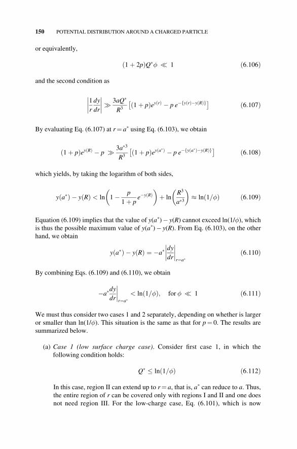
In this case, region II can extend up to r¼ a, that is, a� can reduce to a. Thus,the entire region of r can be covered only with regions I and II and one does
not need region III. For the low-charge case, Eq. (6.101), which is now
150 POTENTIAL DISTRIBUTION AROUND A CHARGED PARTICLE

applicable essentially for the entire region of r, can further be simplified to
give
yðrÞ ¼ Q� ar
1þ r3
2R3� 9r
5R
� �; a � r � R ð6:113Þ
which is independent of p. For the dilute case (�� 1), Eq. (6.113) gives
yðRÞ 0 ð6:114Þ
and becomes essentially a Coulomb potential, namely,
yðrÞ ¼ Q� ar; a � r � R ð6:115Þ
The scaled particle surface potential yo¼ y(a)� y(R)¼ y(a) in case 1 is thus
given by
yo ¼ Q� ð6:116Þ
The above results do not depend on p and agree with those for the completely
salt- free case.
(b) Case 1 (high surface charge case). Consider next case 2, in which the condi-
tion
Q� > lnð1=�Þ ð6:117Þ
is satisfied so that
Q� > �a�dy
dr
����r¼a�
ð6:118Þ
That is, region II cannot extend up to r¼ a. Therefore, the entire region of rcannot be covered only with regions I and II and thus one needs region III
very near the particle surface between r¼ a and r¼ a�, where counterions
are condensed (counter-ion condensation). In region III, y(r) is very high so
that Eq. (6.99) becomes
d2y
dr2¼ 3�Q�
a2ð1þ pÞeyðrÞ ð6:119Þ
By integrating Eq. (6.119), we obtain for the dilute case
yðaÞ ¼ lnQ�
6�ð1þ pÞ� �
ð6:120Þ
EFFECTS OF A SMALL AMOUNT OF ADDED SALTS 151

The value of y(R) can be obtained as follows. In case 2, y(a�)� y(R) hasalready reached its maximum ln(1/�) so we find that Eq. (6.102) becomes
yðrÞ ¼ Q�eff
a
rþ yðRÞ; a� � r � R� ð6:121Þ
where
Q�eff ¼ yða�Þ � yðRÞ ¼ Q�ð1þ pÞeyðRÞ � p
¼ lnð1=�Þ ð6:122Þ
is the scaled effective particle charge and the value of y(R) is given by
yðRÞ ¼ lnlnð1=�Þ þ pQ�
Q�ð1þ �Þ� �
ð6:123Þ
which is obtained from the last equation of Eq. (6.122). We see from
Eq. (6.123) that y(R) tends to zero as p increases. Equation (6.121) implies
that in region II the potential distribution around the particle is a Coulomb
potential produced by the scaled particle charge Q�eff ¼ ln(1/�). In other
words, the particle behaves as if the particle charge were Q�eff instead of Q�
for regions I and II, in which regions Eq. (6.102) may be expressed as
yðrÞ ¼ Q�eff
a
r1þ r3
2R3� 3r
2R
� �þ yðRÞ; a� � r � R ð6:124Þ
The particle surface potential yo¼ y(a)� y(R) in case 2 is found to be, from
Eqs. (6.120) and (6.123),
yo ¼ lnðQ�Þ2
6�flnð1=�Þ þ pQ�g
" #ð6:125Þ
When p¼ 0, Eqs. (6.120), (6.123) and (6.125) all reduce back to results ob-
tained for the completely salt-free case. Also note that the critical value sepa-
rating cases 1 and 2 is ln(1/�), which is the same as that for the completely
salt-free case.
6.5 SPHERICAL SOFT PARTICLE
Consider a dilute suspension of polyelectrolyte-coated spherical colloidal particles
(soft particles) in a salt-free medium containing counterions only. We assume that
the particle core of radius a (which is uncharged) is coated with an ion-penetrable
layer of polyelectrolytes of thickness d. The polyelectrolyte-coated particle has thusan inner radius a and an outer radius b� a + d (Fig. 6.4). We also assume that ion-
ized groups of valence Z are distributed at a uniform density N in the polyelectrolyte
152 POTENTIAL DISTRIBUTION AROUND A CHARGED PARTICLE

layer so that the charge density in the polyelectrolyte layer is given by ZeN, where eis the elementary electric charge. The total charge amount Q of the particle is thus
given by
Q ¼ 4
3pðb3 � a3ÞZeN ð6:126Þ
We assume that each sphere is surrounded by a spherical free volume of radius R(Fig. 6.4), within which counterions are distributed so that electroneutrality as a
whole is satisfied. The particle volume fraction � is given by
� ¼ ðb=RÞ3 ð6:127Þ
In the following we treat the case of dilute suspensions, namely,
� � 1 or b=R � 1 ð6:128Þ
We denote the electric potential at a distance r from the center O of one particle by
c(r). Let the average number density and the valence of counterions be n and �z,respectively. Then from the condition of electroneutrality in the free volume,
we have
Q ¼ 4
3pðb3 � a3ÞZeN ¼ 4
3pðR3 � a3Þzen ð6:129Þ
FIGURE 6.4 A polyelectrolyte-coated spherical particle (a spherical soft particle) in
a free volume of radius R containing counterions only. a is the radius of the particle core.
b¼ aþ d. d is the thickness of the polyelectrolyte layer covering the particle core. (b/R)3
equals the particle volume fraction �. From Ref. [9].
SPHERICAL SOFT PARTICLE 153

which gives
ZN
zn¼ R3 � a3
b3 � a3ð6:130Þ
We set c(r)¼ 0 at points where the counter-ion concentration equals its average
value n so that the volume charge density r(r) resulting from counterions equals
its average value (�zen). We assume that the distribution of counterions obeys a
Boltzmann distribution, namely,
rðrÞ ¼ �zen exp ��zecðrÞkT
� �¼ �zen exp
zecðrÞkT
� �ð6:131Þ
The Poisson equations for the electric potential c(r) in the region inside and outsidethe polyelectrolyte layer are then given by
d2cðrÞdr2
þ 2
r
dcðrÞdr
¼ � rðrÞereo
� ZeN
ereo; a < r < b ð6:132Þ
d2cðrÞdr2
þ 2
r
dcðrÞdr
¼ � rðrÞereo
; b < r < R ð6:133Þ
Here we have assumed that the relative permittivity er takes the same value in the
medium inside and outside the polyelectrolyte layer. By combining Eqs. (6.131)–
(6.133), we obtain the following Poisson–Boltzmann equations:
d2y
dr2þ 2
r
dy
dr¼ k2 ey � ZN
zn
� �; a < r < b ð6:134Þ
d2y
dr2þ 2
r
dy
dr¼ k2ey; b < r < R ð6:135Þ
where y(r)¼ zec(r)/kT is the scaled potential and
k¼ z2e2n
ereokT
� �1=2
¼ Zze2Nðb3� a3ÞereokTðR3� a3Þ
� �1=2¼ 3zeQ
4pereokTðR3� a3Þ� �1=2
¼ 3Q�bR3� a3
� �1=2
ð6:136Þis the Debye–H€uckel parameter in the present system. In Eq. (6.136), Q� is the
scaled particle charge defined by
Q� ¼ Q
4pereobze
kT
� �ð6:137Þ
154 POTENTIAL DISTRIBUTION AROUND A CHARGED PARTICLE

By using Eq. (6.130), we can rewrite Eq. (6.134) as
d2y
dr2þ 2
r
dy
dr¼ k2 ey� R3� a3
b3� a3
� �� �¼ 3Q�b
R3ey� R3� a3
b3� a3
� �� �; a< r< b ð6:138Þ
which becomes for the dilute case
d2y
dr2þ 2
r
dy
dr¼ k2 ey� R3
b3� a3
� �¼ 3Q�b
R3ey� R3
b3� a3
� �; a< r< b ð6:139Þ
The boundary conditions for y are expressed as
dy
dr
����r¼a
¼ 0 ð6:140Þ
dy
dr
����r¼R
¼ 0 ð6:141Þ
yðb�Þ ¼ yðbþÞ ð6:142Þ
dy
dr
����r¼b�
¼ dy
dr
����r¼bþ
ð6:143Þ
We derive approximate solutions to Eqs. (6.135) and (6.139) for the dilute case by
using an approximation method described in Ref. [5], as follows.
(a) Case 1 (low surface charge case). If the condition
Q� � lnð1=�Þ ð6:144Þ
is satisfied, Eq. (6.135) can be approximated by
d2y
dr2þ 2
r
dy
dr¼ k2; b < r < R ð6:145Þ
from which we have
yðrÞ ¼ Q� br
1þ r3
2R3� 9r
5R
� �; ðb � r � RÞ ð6:146Þ
SPHERICAL SOFT PARTICLE 155

or
cðrÞ ¼ Q
4pereor1þ r3
2R3� 9r
5R
� �; ðb � r � RÞ ð6:147Þ
For the dilute case (�� 1), Eq. (6.147) can be approximated well by an un-
screened Coulomb potential of a sphere carrying charge Q, namely,
cðrÞ ¼ Q
4pereor; ðb � r � RÞ ð6:148Þ
That is, in the low charge case, the potential is essentially the same as if con-
terions were absent. This suggests that the potential inside the polyelectrolyte
layer is also approximately the same as if conterions were absent. If counter-
ions are absent, then Eq. (6.139) becomes
d2y
dr2þ 2
r
dy
dr¼ � k2R3
b3 � a3¼ � 3bQ�
b3 � a3; ða < r < bÞ ð6:149Þ
with the solution
yðrÞ ¼ Q�b3
ðb3 � a3Þ3
2� r2
2b2� a3
b2r
� �; ða � r � bÞ ð6:150Þ
or
cðrÞ ¼ Qb2
4pereoðb3 � a3Þ3
2� r2
2b2� a3
b2r
� �; ða � r � bÞ ð6:151Þ
If the surface potential cs of the polyelectrolyte-coated particle is identified
as cs¼c(b)�c(R), then we find that for the dilute case
cðRÞ ¼ 0 ð6:152Þ
co ¼ cðbÞ ¼ Q
4pereobð6:153Þ
or
yðRÞ ¼ 0 ð6:154Þ
yo ¼ Q� ð6:155Þ
156 POTENTIAL DISTRIBUTION AROUND A CHARGED PARTICLE
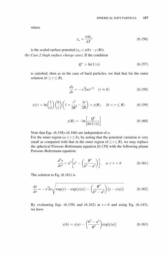
where
yo ¼zeco
kTð6:156Þ
is the scaled surface potential (yo¼ y(b)� y (R)).
(b) Case 2 (high surface charge case). If the condition
Q� > lnð1=�Þ ð6:157Þ
is satisfied, then as in the case of hard particles, we find that for the outer
solution (b � r � R),
dy
dr¼ �
ffiffiffi2
pkey=2 ðr bÞ ð6:158Þ
yðrÞ ¼ ln1
�
� �b
r
� �1þ r3
2R3� 3r
2R
� �þ yðRÞ; ðb < r � RÞ ð6:159Þ
yðRÞ ¼ �lnQ�
lnð1=�Þ� �
ð6:160Þ
Note that Eqs. (6.158)–(6.160) are independent of a.For the inner region (a� r� b), by noting that the potential variation is very
small as compared with that in the outer region (b� r�R), we may replace
the spherical Poisson–Boltzmann equation [6.139] with the following planar
Poisson–Boltzmann equation:
d2y
dr2¼ k2 ey � R3
b3 � a3
� �� �; a < r < b ð6:161Þ
The solution to Eq. (6.161) is
dy
dr¼ �
ffiffiffi2
pk
ffiffiffiffiffiffiffiffiffiffiffiffiffiffiffiffiffiffiffiffiffiffiffiffiffiffiffiffiffiffiffiffiffiffiffiffiffiffiffiffiffiffiffiffiffiffiffiffiffiffiffiffiffiffiffiffiffiffiffiffiffiffiffiffiffiffiffiffiffiffiffiffiffiffiffiffiffiffiffiffiffiffiffiffiffiffiexpðyÞ � expðyðaÞÞ � R3
b3 � a3
� �y� yðaÞf g
sð6:162Þ
By evaluating Eqs. (6.158) and (6.162) at r¼ b and using Eq. (6.143),
we have
yðbÞ ¼ yðaÞ � b3 � a3
R3
� �exp yðaÞ½ � ð6:163Þ
SPHERICAL SOFT PARTICLE 157

Equation (6.162) can further be integrated to yield
� ffiffiffi2
pkðr � aÞ ¼
Z y
yðaÞ
dyffiffiffiffiffiffiffiffiffiffiffiffiffiffiffiffiffiffiffiffiffiffiffiffiffiffiffiffiffiffiffiffiffiffiffiffiffiffiffiffiffiffiffiffiffiffiffiffiffiffiffiffiffiffiffiffiffiffiffiffiffiffiffiffiffiffiffiffiffiffiffiffiffiffiffiffiffiffiffiffiffiffiffiffiffiffiffiffiffiffiffiffiffiffiexpðyÞ � expðyðaÞÞ � ðR3=ðb3 � a3ÞÞfy� yðaÞg
q
�2ffiffiffiffiffiffiffiffiffiffiffiffiffiffiffiffiffiyðaÞ � y
pffiffiffiffiffiffiffiffiffiffiffiffiffiffiffiffiffiffiffiffiffiffiffiffiffiffiffiffiffiffiffiffiffiffiffiffiffiffiffiffiffiffiffiffiffiffiffiffiffiffiR3=ðb3 � a3Þ � exp½yðaÞ�
qð6:164Þ
where we have expanded the integrand around y¼ y(a) and carried out the
integration, since the largest contribution to the integrand comes from the
region near y¼ y(a). Equation (6.164) yields
yðrÞ ¼ yðaÞ þ eyðaÞ � R3
ðb3 � a3Þ
� �k2ðr � aÞ2 ð6:165Þ
which may also be obtained by directly expanding y(r) around r¼ a on the
basis of Eq. (6.139). From Eqs. (6.163) and (6.165) (evaluated at r¼ b) weobtain
yðaÞ ¼ ln3Q�bR3
f3Q�bðb� aÞ þ 2ðb2 þ abþ a2Þgðb2 þ abþ a2Þ
� �ð6:166Þ
and
yðbÞ ¼ ln3Q�bR3
f3Q�bðb� aÞ þ 2ðb2 þ abþ a2Þgðb2 þ abþ a2Þ
� �
� 3Q�bðb� aÞf3Q�bðb� aÞ þ 2ðb2 þ abþ a2Þg
ð6:167Þ
Thus, we find that the scaled surface potential yo¼ y(b)� y(R) is given by
yo ¼ ln3Q�2bR3
lnð1=�Þf3Q�bðb� aÞ þ 2ðb2 þ abþ a2Þgðb2 þ abþ a2Þ
� �
� 3Q�bðb� aÞf3Q�bðb� aÞ þ 2ðb2 þ abþ a2Þg
ð6:168Þ
The Poisson–Boltzmann equations (6.135) and (6.139) subject to boundary condi-
tions (6.140)–(6.143) can be solved numerically with Mathematica to obtain
the potential distribution y(x). The results of some calculations for the potential
158 POTENTIAL DISTRIBUTION AROUND A CHARGED PARTICLE

distribution are given in Figs 6.5 and 6.6, which demonstrate y(r) for Q�¼ 5 (low
charge case) and 50 (high charge case) at �¼ 10�6 and a/b¼ 0.9. Figure 6.5 shows
the exact numerical results for the inner solution (a � r � b) in comparison with
approximate results (Eq. (6.150) for Q�¼ 5 and Eq. (6.165) for Q�¼ 50), showing
FIGURE 6.6 Distribution of the scaled electric potential y(r) outside the polyelectrolyte
layer (b� r�R) at �¼ 10�6 and a/b¼ 0.9 for Q�¼ 5 (low charge case) and Q�¼ 50 (high
charge case). Approximate results (Eq. (6.146) for Q�¼ 5 and Eq. (6.159) for Q�¼ 50) agree
with exact results within the linewidth. From Ref. [9].
FIGURE 6.5 Distribution of the scaled electric potential y(r) within the polyelectrolyte
layer (a� r� b) at �¼ 10�6 and a/b¼ 0.9 for Q�¼ 5 (low charge case) and Q�¼ 50 (high
charge case). Solid curves, exact results; dotted curves, approximate results (Eq. (6.150) for
Q�¼ 5 and Eq. (6.165) 6. for Q�¼ 50). From Ref. [9].
SPHERICAL SOFT PARTICLE 159

good agreement between numerical and approximate results. Figure 6.6 shows the
exact numerical results for the outer region b� r�R, which agree with approxi-
mate results (Eq. (6.146) for Q�¼ 5 and Eq. (6.159) for Q�¼ 50) within the line-
width. It is seen that for the high charge case (Q�¼ 50) the potential outside
the polyelectrolyte layer decreases very sharply near the surface of the poly-
electrolyte layer (r¼ b) and essentially constant (y(r) y(R)) except in the region
very near the polyelectrolyte layer.
In Fig. 6.7, the scaled surface potential ys¼ y(b)� y(R) is plotted as a func-
tion of Q� at a/b¼ 0.5 for �¼ 10�3, 10�6, and 10�9. We see that as in the case
of a rigid particle, there is a certain critical value separating the low charge
case and the high charge case. Approximate results (Eq. (6.155) for the low
charge case and Eq. (6.168) for the high charge case) are also shown in Fig.
6.7. An approximate expression for the critical value Q�cr is given by (see Eqs.
(6.144) and (6.157))
Q�cr ¼ lnð1=�Þ ð6:169Þ
When Q��Q�cr (low charge case), the surface potential may be approximated by
Eq. (6.155), which is the unscreened Coulomb potential for the case where coun-
terions are absent. The surface potential ys is proportional to Q� in this case. When
Q�>Q�cr (high charge case), the surface potential can be approximated by
FIGURE 6.7 Scaled surface potential yo¼ zeco/kT, defined by yo� y(b)� y(R), as a func-tion of the scaled charge Q�= (ze/kT)Q/4pereob at a/b¼ 0.5 for various values of the particle
volume fraction �. Solid lines represent exact numerical results. The dashed line, which
passes through the origin (yo¼ 0 and Q�¼ 0), is approximate results calculated by an un-
screened Coulomb potential, Eq. (6.155) (low charge case) and dotted lines by Eq. (6.168)
(high charge case). Closed circles correspond to the approximate critical values Qcr� of
the scaled particle charge Q� separating cases, the low and high charge cases, given by
Qcr�¼ ln(1/�). From Ref. [9].
160 POTENTIAL DISTRIBUTION AROUND A CHARGED PARTICLE

Eq. (6.168). The dependence of the surface potential ys upon the particle charge
Q� is considerably suppressed since the counterions are accumulated within and
near the polyelectrolyte layer (counter-ion condensation).
For the limiting case of a¼ b (in which case the polyelectrolyte-coated particle
becomes a rigid particle with no polyelectrolyte layer), Eq. (6.168) tends to
yo ¼ lnQ�2
6� lnð1=�Þ� �
ð6:170Þ
which agrees with Eq. (6.50) for the surface potential of a rigid particle in a salt-free
medium. For the case where a � b and Q is high, Eq. (6.168) tends to
yo ¼ lnQ�
expð1Þ� lnð1=�Þð1� a3=b3Þ
� �ð6:171Þ
When a¼ 0, in particular, the polyelectrolyte-coated particle becomes a spherical
polyelectrolyte with no particle core. In this case, Eq. (6.171) tends to
ys ¼ lnQ�
expð1Þ� lnð1=�Þ� �
ð6:172Þ
FIGURE 6.8 Scaled surface potential yo¼ zeco/kT, defined by yo� y(b)� y(R), as a func-tion of the ratio d/a of the thickness d¼ b� a of the polyelectrolyte layer to the radius a of
the particle core at �¼ 10�6 for Q�¼ 5 (low charge case) and Q�¼ 50 (high charge case).
Solid lines represent exact numerical results. The dotted lines are approximate results calcu-
lated by an unscreened Coulomb potential (Eq. (6.155)) for the low charge case and by Eq.
(6.168) for the high charge case. From Ref. [9]
SPHERICAL SOFT PARTICLE 161

Figure 6.8 shows yo as a function of the ratio d/a of the polyelectrolyte layer thick-
ness d to the core radius a for two values of Q� (5 and 50) at �¼ 10�6. Note that as
d/a tends to zero, the polyelectrolyte-coated particle becomes a hard sphere with
no polyelectrolyte layer, while as d/a tends to infinity, the particle becomes a
spherical polyelectrolyte with no particle core. Approximate results calculated with
Eq. (6.155) for Q�¼ 5 (low charge case) and Eq. (6.168) for Q�¼ 50 (high charge
case) are also shown in Fig. 6.8. Agreement between exact and approximate results
is good. For the low charge case, the surface potential is essentially independent
of d and is determined only by the charge amount Q�. In the example given in
Fig. 6.8, for the high charge case, the particle behaves like a hard particle with no
polyelectrolyte layer for d/a � 10�3 and the particle behaves like a spherical poly-
electrolyte for d/a � 1.
REFERENCES
1. R. M. Fuoss, A. Katchalsky, and S. Lifson, Proc. Natl. Acad. Sci. USA 37 (1951) 579.
2. T. Afrey, P. W. Berg, and H. Morawetz, J. Polym. Sci. 7 (1951) 543.
3. N. Imai and F. Oosawa, Busseiron Kenkyu 52 (1952) 42; 59 (1953) 99 (in Japanese).
4. F. Oosawa, Polyelectrolytes, Dekker, New York, 1971.
5. H. Ohshima, J. Colloid Interface Sci. 247 (2002) 18.
6. H. Ohshima, J. Colloid Interface Sci. 255 (2002) 202.
7. H. Ohshima, Theory of Colloid and Interfacial Electric Phenomena, Elsevier/Academic
Press, Amsterdam, 2006.
8. H. Ohshima, Colloid Polym. Sci. 282 (2004) 1185.
9. H. Ohshima, J. Colloid Interface Sci. 268 (2003) 429.
162 POTENTIAL DISTRIBUTION AROUND A CHARGED PARTICLE


![Colloids and Surfaces B: Biointerfaces - CAS · Colloids and Surfaces B: Biointerfaces 88 (2011) ... such as medicine/pharmacy [1–3], chemical engineering ... styrene as co-monomer](https://img.pdfslide.net/doc/110x75/5b2550217f8b9af0278b4666/colloids-and-surfaces-b-biointerfaces-colloids-and-surfaces-b-biointerfaces.jpg)
![Colloids and Surfaces B: Biointerfaces Colloids Surfaces B... · Colloids and Surfaces B: Biointerfaces 116 (2014) ... antibiotics [3–6]. Their broad ... Alamethicin is most effective](https://img.pdfslide.net/doc/110x75/5a94ecce7f8b9a9c5b8c50e4/colloids-and-surfaces-b-colloids-surfaces-bcolloids-and-surfaces-b-biointerfaces.jpg)